Abstract

We considered a surgery, called $la$-disk surgery, that can be applied to a Lagrangian surface $L$ at the presence of a Lagrangian attaching disk $D$, to obtain a new Lagrangian surface $L^{\prime}:=\eta_{D}(L)$ which is always smoothly isotopic to $L$. We showed that this type of surgery includes all even generalized Dehn twists as constructed by Seidel. We also constructed a new symplectic invariant, called $y$-index, for orientable closed Lagrangian surfaces immersed in a parallelizable symplectic 4-manifold $W$. With $y$-index we proved that $L$ and $\eta_{D}(L)$ are not Hamiltonian isotopic under this setup. We also obtained new examples of smoothly isotopic nullhomologous Lagrangian tori which are not Hamiltonian isotopic pairwise.

1 Introduction

1.1 Isotopy of Lagrangian surfaces

A Lagrangian submanifold in a symplectic manifold $(W,\omega)$ is a submanifold $L\overset{\iota}{\hookrightarrow}W$ such that $\iota^{*}\omega=0$ and $\dim L=\frac{1}{2}\dim W$. In symplectic topology Lagrangian submanifolds distinguish themselves from other types of submanifolds in that, though the symplectic form $\omega$ vanishes on them, their mere presence uniquely determine the nearby symplectic structure, as stated in Weinstein’s Lagrangian neighborhood theorem [20] (see also [14]):

Theorem 1.1.1 (Lagrangian neighborhood theorem).

Let $L$ be an embedded compact Lagrangian submanifold of a symplectic manifold $(W,\omega)$. Then there exist tubular neighborhoods $U\subset W$ of $L$, $V\subset T^{*}L$ of the zero section $L_{0}=L\subset T^{*}L$, and a diffeomorphism $\phi:V\to U$ such that $\phi(L_{0})=L$ and $\phi^{*}\omega=\omega_{can}$, where $\omega_{can}$ is the canonical symplectic structure of the cotangent bundle $T^{*}L$.

In symplectic category one would like to classify Lagrangian submanifolds up to symplectic isotopies or even Hamiltonian isotopies. Two Lagrangian submanifolds $L,L^{\prime}$ are symplectically isotopic if there exist a family of diffeomorphisms $\phi_{t}$, $t\in[0,1]$, $\phi_{0}=id$, $\phi_{t}^{*}\omega=\omega$ for all $t\in[0,1]$, such that $\phi_{1}(L)=L^{\prime}$. The maps $\phi_{t}$, being symplectomorphisms, are generated by symplectic vector fields $X_{t}$ defined by the condition $d(\iota(X_{t})\omega)=0$. If moreover, $\iota(X_{t})\omega=-dH_{t}$ is exact, then $L,L^{\prime}$ are Hamiltonian isotopic. When $H^{1}(W,\mathbb{R})=0$, symplectically isotopic Lagrangian surfaces in $W$ are automatically Hamiltonian isotopic. Clearly symplectically isotopic Lagrangian submanifolds are smoothly isotopic if we drop the condition of $\phi_{t}$ being $\omega$-preserving. Note that an alternative definition for $L$ and $L^{\prime}$ being smoothly isotopic is if $L=L_{0}$ and $L^{\prime}=L_{1}$ can be included in a smooth $1$-parameter family of submanifolds $L_{t}\subset W$, $t\in[0,1]$, and all $L_{t}$ diffeomorphic to $L$. The family $L_{t}$ is called a smooth isotopy between $L$ and $L^{\prime}$. We mention here that there is a middle ground in between called Lagrangian isotopy where we request that all $L_{t}$ are Lagrangian too.

Smoothly isotopic Lagrangian surfaces need not be symplectically isotopic. It is our goal here to better understand the subtle difference between symplectic isotopy and smooth isotopy and we will focus on the case when the Lagrangian submanifold is a 2-dimensional surface, i.e, a Lagrangian knot as in [9].

For earlier results concerning smoothly but not symplectically isotopic Lagrangian surfaces, please see [4, 19, 10, 11, 1, 23, 13]. Here we consider a different approach. We ask the following two questions:

Question 1.1.2.

Find a procedure that can be applied to a given Lagrangian surface $L$ (as general as possible) to yield a new one $L^{\prime}$ which is always smoothly isotopic to $L$ but potentially not symplectically so.

Question 1.1.3.

Construct a symplectic isotopy invariant for Lagrangian surfaces and use it to show that $L,L^{\prime}$ as in Question 1.1.2 are not symplectically isotopic.

1.2 Main constructions and results

To answer Question 1.1.2 we consider a Lagrangian surface $L$ which admits an Lagrangian attaching disk ($la$-disk) $D$. We classify $D$ into three types: parabolic, hyperbolic, and elliptic, according to the homology/homotopy type of the boundary $C:=\partial D\subset L$ in $L$. Each type of a $la$-disk $D$ also comes with two flavors which we call the polarity (see Definition 2.1.4) of $D$. With $D$ we construct the $la$-disk surgery $\eta_{D}$ which can be applied to $L$ to get a new Lagrangian surface $L^{\prime}:=\eta_{D}(L)$. Roughly speaking this surgery cut out a collar neighborhood of $C$ in $L$ and glue in a different Lagrangian annulus along the boundary. We remark here that our surgery here is closely related to the Lagrangian surgery as defined in [17]. In [17] a 2-dimensional Lagrangian surgery is to remove a positive self-intersection point of a Lagrangian surface. In contrast our $la$-disk surgery is about the transition between the two Lagrangian surfaces $L,L^{\prime}$ resulting from different ways of de-singularizing a Lagrangian surface at a positive self-intersection point.

We obtained the following results among other things:

• The resulting Lagrangian surface $L^{\prime}:=\eta_{D}(L)$ is smoothly isotopic to $L$ (Proposition 2.3.1).

  Dually, $L^{\prime}$ has a $la$-disk $D^{\prime}$ of the same type as $D$ but with different relative polarity, and $\eta_{D^{\prime}}(L^{\prime})=L$. Note the actual surface $L^{\prime}:=\eta_{D}L$ depends on the size of the surgery, nevertheless its Lagrangian isotopy class is unique.

• If $L$ is monotone then under suitable conditions $L^{\prime}$ is also monotone (Proposition 2.5.1).

  As examples, we have (i) if $L\subset\mathbb{R}^{4}$ is a Chekanov torus as defined in [4], then $L^{\prime}$ is a monotone Clifford torus; (ii) if $L\subset T^{*}S^{2}$ is a monotone Clifford torus, and $D$ is a unstable (see Definition 2.1.5) parabolic $la$-disk of $L$, then (up to scaling) $\eta_{D}(L)$ is the non-displaceable torus constructed in [1].

• If $L$ is a null-homologous Lagrangian torus, then the maximal number of mutually disjoint $la$-disks of $L$ imposes some restriction on the homology of $W$ (Proposition 2.2.4, Corollary 2.2.6).

• If $D$ is elliptic then $\eta_{D}$ is equal to the square of a positive or negative generalized Dehn twist as considered in [19], where the sign is determined by the polarity of $D$ (Proposition 2.4.3).

The $la$-disk surgery provides a general way of potentially changing the symplectic isotopy type of a Lagrangian surface without affecting its smooth isotopy type. On the other hand, $la$-disks seems intimately related to the build-up of a symplectic $4$-manifold around a Lagrangian surface. For example, in the integrable system considered in Section 5.1.3, a Chekanov torus $L$ lives in the boundary of the Stein domain diffeomorphic to $S^{1}\times B^{3}$ the product of $S^{1}$ with a $3$-ball, $\mathbb{R}^{4}$ can be obtained by attaching to $S^{1}\times B^{3}$ a Lagrangian $2$-handle such that the core disk of the $2$-handle is a stable parabolic $la$-disk of $L$ in $\mathbb{R}^{4}$. Similarly, $T^{*}S^{2}$ is obtained by attaching along the boundary $S^{3}=\partial B^{4}$ of a $4$-ball a Lagrangian $2$-handle whose core disk is again a stable parabolic $la$-disk in $T^{*}S^{2}$ of a monotone Clifford torus $L^{\prime}\subset S^{3}$.

For Question 1.1.3 we were able to construct a new symplectic isotopy invariant, called $y$-index, for orientable compact Lagrangian surfaces immersed in $W$ provided that $W$ is parallelizable.

First of all, if $W$ is parallelizable then we can fix a $\omega$-compatible unitary framing $\EuFrak{f}:=(J,u,v)$, where $J$ is an $\omega$-compatible almost complex structure over $W$, $(u,v)$ is a $J$-complex unitary basis of $TW$. The framing $\EuFrak{f}$ allows us to define the projected Lagrangian Gauss map (PLG-map)

$$g^{\prime}_{L}:L\to\mathbb{P}(K^{\prime})\cong S^{2}$$

for any oriented immersed Lagrangian surface $L$ in $W$. Here $\mathbb{P}(K^{\prime})$ is an $S^{2}$-family of oriented Lagrangian planes which are $K^{\prime}$-complex for some orthogonal complex structure $K^{\prime}$. If $L$ is also closed then we define the $\mu_{2}$-index of $L$ relative to $\EuFrak{f}$ to be the degree of the map $g^{\prime}_{L}$:

$$\mu_{2}(L;\EuFrak{f}):=\deg(g^{\prime}_{L})\in\mathbb{Z}.$$

This $\mu_{2}$-index seems classical but we do not know if it has appeared elsewhere in the literature.

We obtained the following results concerning $\mu_{2}$:

Proposition 1.2.1.

1. $\mu_{2}(L;\EuFrak{f})$ is independent of the orientation of $L$.

2. $\mu_{2}(L;\EuFrak{f})$ depends only on the homotopy class of $\EuFrak{f}$ in $\mathcal{F}^{\omega}$ the set of all $\omega$-compatible unitary framings.

3. $\mu_{2}(L,\EuFrak{f})$ is invariant under the $la$-disk surgery.

Moreover, if $H_{1}(W,\mathbb{Z})=0=H_{3}(W,\mathbb{Z})$ then $\mathcal{F}^{\omega}$ is connected and $\mu_{2}(L,\EuFrak{f})$ is independent of $\EuFrak{f}$.

Clearly $\mu_{2}$-index is invariant under regular homotopy of immersed Lagrangian surfaces, hence not sensitive enough to distinguish Hamiltonian or symplectic isotopy classes of Lagrangian surfaces. For example, both Chekanov tori and Clifford tori have their $\mu_{2}$-indexes equal to $0$ (see Section 5.1.2).

A closer inspection on the map $g^{\prime}_{L}$ reveals that a $la$-disk surgery seems make some essential change that can be described in terms of the variation of the intersection subspaces between complex planes and Lagrangian planes, leading to the definition of the $y$-index which we sketch below:

The framing $\EuFrak{f}=(J,u,v)$ associates a unique family of $J$-complex line bundles

$$E_{\theta}=u_{\theta}\wedge Ju_{\theta},\quad\theta\in\mathbb{R}/\pi\mathbb{Z},$$

where $u_{\theta}:=u\cos\theta+v\sin\theta$. Let $v_{\theta}:=Ju_{\theta}$. The pair $(u_{\theta},v_{\theta})$ is well-defined up to a simultaneous change of $\pm$-signs. This sign ambiguity however will not hinder our construction below. Observe that $E_{\theta+\frac{\pi}{2}}$ is orthogonal to $E_{\theta}$, so we also denote

$$\theta^{\perp}:=\theta+\frac{\pi}{2}\ \text{ and }\ E^{\perp}_{\theta}:=E_{\theta^{\perp}},\quad\text{for }\theta\in\mathbb{R}\mod\pi.$$

Let $L\subset W$ be an oriented compact immersed Lagrangian surface. Then for any $p\in L$, there exists $\theta,\theta^{\perp}\in\mathbb{R}/\mathbb{Z}$ such that

$$\dim T_{p}L\cap E_{\theta}|_{p}=1=\dim T_{p}L\cap E_{\theta^{\perp}}|_{p}.$$

We call the set

$$\Gamma_{\theta}:=\{p\in L\mid\dim T_{p}L\cap E_{\theta}=1\}$$

the intersection locus of $E_{\theta}$ or the $E_{\theta}$-locus in $L$. It turns out that we can orient a subset $\check{\Gamma}_{\theta}$ of $\Gamma_{\theta}$, call the proper $E_{\theta}$-locus, in a consistent way for all $\theta$ so that the positively oriented proper loci, denoted as $\check{\Gamma}^{+}_{\theta}$, satisfy

$$\check{\Gamma}^{+}_{\theta^{\perp}}=-\check{\Gamma}^{+}_{\theta}=:\check{\Gamma}^{-}_{\theta},$$

with $\check{\Gamma}^{-}_{\theta}$ denotes the negatively oriented $\check{\Gamma}_{\theta}$. Each $E_{\theta}$ comes with a trivialization given by $(u_{\theta},v_{\theta})$, with which we can count the total angle of variation $\alpha^{+}_{\theta}$ (resp. $\alpha^{-}_{\theta}$) in $E_{\theta}$ (resp. in $E_{\theta^{\perp}}$) of the intersection subspace $T_{p}L\cap E_{\theta}$ (resp. $T_{p}L\cap E_{\theta^{\perp}}$) as we traverse all components of $\check{\Gamma}^{+}_{\theta}$ once. The difference

$$\alpha_{\theta}:=\alpha^{+}_{\theta}-\alpha^{-}_{\theta}$$

which we call the relative $E_{\theta}$-phase along $\check{\Gamma}^{+}_{\theta}$ is independent of $\theta$ and is an integral multiple of $2\pi$. Observe that we get the other uniform orientation for all $\check{\Gamma}_{\theta}$ by simultaneously reversing the orientations of all $\check{\Gamma}^{+}_{\theta}$. The sign of $\alpha_{\theta}$ will be revered if we change the uniform orientation.

That $\check{\Gamma}^{+}_{\theta}$ can be uniformly oriented comes from a decomposition of $L$ into a finite number of crossing domains (see Definition 3.4.13) $L_{i}$ $i\in I$, of $g^{\prime}_{L}$, and the existence of a symmetric function $\varepsilon:I\times I\to\{\pm 1\}$ is defined so that $\varepsilon(i,j)\varepsilon(j,k)=\varepsilon(i,k)$ for all $i,j,k\in I$. The choice of a reference crossing domain $L_{i_{0}}\subset L$ determines a uniform orientation of $\check{\Gamma}^{+}_{\theta}$. Choosing another $L_{i}$ gives the same uniform orientation iff $\varepsilon(i_{0},i)=1$.

Fix a reference crossing domain $L_{i_{0}}$ (and hence a uniformly oriented $\check{\Gamma}^{+}_{\theta}$), we define the $y$-index of $L$ to be

$$y(L,q;\EuFrak{f}):=\frac{1}{2\pi}\alpha_{\theta}.$$

Here $q\in L_{i_{0}}$ is a regular point of $g^{\prime}_{L}$, and it is to represent the uniform orientation determined by $L_{i_{0}}$. Clearly $y(L,p,\EuFrak{f})=y(L,q,\EuFrak{f})$ if $p\in L_{i}$ and $q\in L_{j}$ satisfy $\varepsilon(i,j)=1$. We define the absolute $y$-index to be

$$\bar{y}(L;\EuFrak{f}):=|y(L,q;\EuFrak{f})|.$$

For each $i$, the degree $d_{i}\in\mathbb{Z}$ of the restricted PLG-map $g^{\prime}_{L}|_{L_{i}}:L_{i}\to\mathbb{P}(K^{\prime})$ is defined. Let $L_{i_{0}}$ and $q$ be as above. Then $y(L,q,\EuFrak{f})$ can also be expressed as

$$y(L,q;\EuFrak{f})=\sum_{j\in I}\epsilon(i_{0},j)d_{j}.$$

So $y(L,q;\EuFrak{f})$ can be defined by summing up the signed degrees of crossing domains of $L$ relative to a reference crossing domain. It is this extra sign that set the $y$-index apart from the $\mu_{2}$-index.

Given two oriented immersed Lagrangian surfaces $L,L^{\prime}$, suppose that $L\cap L^{\prime}$ contains an open domain $U$ on which $L$ and $L^{\prime}$ induces the same orientation, and suppose that $q\in U$ is a regular value for $g^{\prime}_{L}$ (and hence for $g^{\prime}_{L^{\prime}}$, then a relative $y$-index is defined:

$$y(L^{\prime},L,q;\EuFrak{f}):=y(L^{\prime},q;\EuFrak{f})-y(L,q;\EuFrak{f}).$$

We have the following results:

Theorem 1.2.2.

1. $y(L,q;\EuFrak{f})$ and $y(L^{\prime},L,q;\EuFrak{f})$ are independent of the orientation of $L$ and $L^{\prime}$.

2. For $L,L^{\prime}$ fixed, $y(L,q;\EuFrak{f})$, $\bar{y}(L;\EuFrak{f})$ and $y(L^{\prime},L,q;\EuFrak{f})$ depends only on the path connected components of $\EuFrak{f})$.

3. If $L$ and $L^{\prime}$ are symplectically isotopic, then $\bar{y}(L;\EuFrak{f})=\bar{y}(L^{\prime};\EuFrak{f})$ for $\EuFrak{f}\in\mathcal{F}^{\omega}$.

4. If $L^{\prime}=\eta_{D}(L)$ then

   $$|y(L^{\prime},q;\EuFrak{f})-y(L,q;\EuFrak{f})|=4,$$

When $H_{1}(W,\mathbb{Z})=0=H_{3}(W,\mathbb{Z})$ every $\omega$-compatible almost complex structure $J$, the set of $J$-complex unitary framings $(u,v)$ is path connected. Since the set of all $\omega$-compatible almost complex structures over $W$ is contractible, the set $\mathcal{F}^{\omega}$ is connected. Then the $y$-index $y(L,q;\EuFrak{f})$ is independent of $\EuFrak{f}\in\mathcal{F}^{\omega}$ and is invariant under symplectomorphisms of $L$. In this case we will usually omit $\EuFrak{f}$ and simply denote the $y$-index of $L$ as $y(L,q)$, and $\bar{y}(L;\EuFrak{f})$ as $\bar{y}(L)$, etc..

By computing the relative $y$-index we reproved that iterations of the generalized Dehn twist can produce an infinite number of smoothly isotopic Lagrangian surfaces representing distinct symplectic/Hamiltonian isotopy classes.

Theorem 1.2.3.

Let $W$ be the plumbing of the cotangent bundles of a smooth orientable surface $L$ and a sphere $S$ at their intersection point. Let $L^{n}:=\tau^{2n}_{S}(L)$ denote the Lagrangian surface in $W$ obtained by applying the $2n$-generalized Dehn twist along $S$ to $L$, $n\in\mathbb{Z}$, $L^{0}=L$.Then for a suitable common point $q$ of $L^{m}$’s,

$$y(L^{m},L^{n},q;\EuFrak{f})=4(m-n),\quad m,n\in\mathbb{Z}.$$

In particular,

$$y(L^{n},L,q;\EuFrak{f})=-4n,\quad n\in\mathbb{Z}.$$

This implies that there are infinitely many Lagrangian surfaces in $W$ which are pairwise Hamiltonian non-isotopic, but all smoothly isotopic.

Let $W_{n}$ denote the cotangent bundle of the $A_{n}$-configuration of $n$’s $2$-spheres, or equivalently, the pluming of cotangent bundles $T^{*}S_{j}$ of $n$’s $2$-spheres $S_{1},...,S_{n}$, so that in $W_{n}$, $S_{i}\cap S_{j}=\emptyset$ unless $j=i+1$, $S_{i}$ intersects transversally with $S_{i+1}$ and in one point. We call $W_{n}$ the $A_{n}$-manifold. Observe that the above result also applies to the plumbing $T^{*}L$ with $W_{n}$ for $n\geq 2$. We remark here that a relevant result was proved by Seidel [19] by way of Lagrangian Floer homology.

The $la$-disk surgery and the relative $y$-index enable us to construct new nullhomologous monotone Lagrangian tori beyond the known ones.

Theorem 1.2.4.

Let $W_{n}$ be the $A_{n}$-manifold, $n\geq 0$, $W_{0}=\mathbb{R}^{4}$. Then on $W_{n}$ there are $n+2$ smoothly isotopic nullhomologous monotone Lagrangian tori, $T_{-1},T_{0},T_{1},...,T_{n}$, with a common domain containing a regular point $q$, such that

$$y(T_{k},T_{j},q)=4(j-k),\quad-1\leq k,j\leq n,$$

hence are pairwise Hamiltonian (and symplectically) non-isotopic.

Note that $T_{-1}$ is a Chekanov torus, $T_{0}$ a Clifford torus, and $T_{1}$ is Hamiltonian isotopic to the torus in $T^{*}S^{2}$ constructed in [1].

With $y$-index and its relative version we reproved earlier examples of smooth but not symplectically isotopic monotone Lagrangian tori obtained by Chekanov [4] and Albers-Frauenfelder [1], and spheres by Seidel [19]. Their methods include symplectic capacities [6, 7, 21, 22] applied in [4] and Lagrangian (intersection) Floer cohomology [15, 16, 18, 12] used in [19, 1]. We remark here that by computing superpotentials Auroux [2] proved that the monotone Clifford torus and Chekanov torus are not Hamiltonian isotopic in $\mathbb{C}P^{2}$. Complement to current methods, our $y$-index provides an alternative and simpler way of distinguishing Lagrangian surfaces in symplectic $4$-manifolds with vanishing Chern classes. Extension of the $y$-index to general symplectic $4$-manifolds is yet to be explored.

It is expected that a contact version of the $la$-disk surgery can be defined for Legendrian surfaces in a contact $5$-manifold $(M,\xi)$, and the same to the $y$-index provided that the contact distribution $\xi$ is parallelizable. We also expect that both the $la$-disk surgery and the $y$-index can be generalized to Lagrangian submanifolds immersed in higher dimensional parallelizable symplectic manifolds.

1.3 Outline of this paper

This paper is organized as follows: In Section 2.1 we introduce the notion of a Lagrangian attaching disk ($la$-disk) and analyze the types of such disks. A standard model for a $la$-disk is established in Section 2.2 to define the $la$-disk surgery $\eta_{D}$ in Section 2.3 and to compare $\eta_{D}$ with the generalized Dehn twists $\tau^{n}_{S}$ in Section 2.4. In Section 2.5 we study the effect of $\eta_{D}$ on Maslov class, Liouville class and monotonicity of a Lagrangian surface. In Section 3.1 we consider an equivariant factorization of oriented Lagrangian Grassmannian $\Lambda^{+}$. In Section 3.2 the intersection loci between complex and Lagrangian planes are analyzed and applied to define a coordinate system for $\Lambda^{+}$ in Section 3.3 and to study maps into $\mathbb{P}(K^{\prime})$ in Section 3.4. In Section 3.4 we define crossing $p$-curves and analyze their deformations. Also defined are crossing domains which will be used to define the $y$-index in Section 4.3. Staring from Section 4.1 we will work with parallelizable symplectic 4-manifolds. The definitions and basic properties of the $\mu_{2}$-index and the $y$-index are presented in Section 4.2 and Section 4.3 respectively. Effects of a $la$-surgery on both indexes are discussed in Section 4.4. Examples are computed in Section 5. In Section 5.1 indexes of tori and Whitney spheres in $\mathbb{R}^{4}$ are determined. Indexes of the zero section of $T^{*}S^{2}$ are obtained in Section 5.2. Section 5.3 is devoted to prove Theorem 1.2.3, and Section 5.4 Theorem 1.2.4.

Acknowledgments.  Part of the work was done during the author’s visit at University of California, Berkeley in 2009-2010, which was partially founded by NSC grants 98-2918-I-008-003 and 99-2115-M-008-005-MY2. The author would like to thank Department of Mathematics of UC Berkeley and in particular Professor Robion Kirby for their hospitality.

2 Surgery of a Lagrangian surface

Lagrangian surgery, viewed as attaching Lagrangian handlebodies along contact boundary, is an important ingredient in the construction/decomposition of of Stein manifolds [8]. In a different meaning it was defined by Polterovich in [17] as a Lagrangian de-singularization procedure. In fact, it was already hidden in the Hamiltonian integrable system literature (see for example [5, 3]) and is responsible for the monodromy of the integrable system. Yet its effect on isotopy of Lagrangian surfaces (the so called Lagrangian knots) has not been fully explored, and this is the direction we will pursue here. We will consider a 2-dimensional Lagrangian surgery as a surgery on a Lagrangian surface in the presence of an embedded Lagrangian attaching disk.

Recall that a submanifold $\iota:C\hookrightarrow W$ of a symplectic manifold $(W,\omega)$ is called isotropic if $\iota^{*}\omega=0$. One dimensional submanifolds are always isotropic. For an isotropic submanifold $C$ we denote

$$(TC)^{\omega}:=\{v\in T_{C}W\mid v\in T_{p}W\text{ for some $p\in C$},\ \omega(v,v^{\prime})=0\ \forall v^{\prime}\in T_{p}C\}.$$

Then $(TC)^{\omega}$ is a vector subbundle of rank $\dim W-\dim C$ over $T_{C}W$, and it contains $TC$ as its subbundle. The quotient bundle

$$N^{\omega}_{C}:=(TC)^{\omega}/TC$$

is a symplectic vector bundle over $C$, called the symplectic normal bundle of $C$ in $W$.

We will also denote the normal bundle of $C\subset D$ by $N_{C/D}$ when $C$ is viewed as a submanifold of a manifold $D$.

2.1 Lagrangian attaching disk

Let $L\subset(W,\omega)$ be a closed Lagrangian surface immersed in a symplectic 4-manifold $(W,\omega)$.

Definition 2.1.1.

A closed embedded Lagrangian disk $D\subset W$ is called a Lagrangian attaching disk ($la$-disk) of $L$ if

1. $C:=\partial D=D\cap L$, and

2. $D\pitchfork_{C}L$, i.e. $D$ is transversal to $L$ along $C$ in the sense that the normal bundles $N_{C/D}$ and $N_{C/L}$ are transversal along $C$, or equivalently, the intersection $L\cap D=C$ is clean, i.e. $T_{C}L\cap T_{C}D=TC$.

We call $C\subset L$ a vanishing cycle of $L$ if there exists a $la$-disk $D$ of $L$ with $\partial D=C$.

The following are two simple propositions regarding a vanishing cycle of $L$ and its neighborhood.

Proposition 2.1.2.

If $C$ is a vanishing cycle of $L\subset W$ then

1. $C=\partial D\subset L$ is $\omega$-exact, and

2. the Maslov index of the loop of Lagrangian planes $T_{C}L$ ($C$ is oriented in either way) with respect to $[D]\in H_{2}(W,L;\mathbb{Z})$ is

   $$\mu(T_{C}L,D)=\mu(T_{C}D,D)=0.$$

In particular, if $c_{1}(W)=0$ then $\mu(T_{C}L)=0$ is well-defined, independent of the choice of a la-disk $D$ with $\partial D=C$.

Proposition 2.1.3.

The outward normal vector field $\nu$ of a la-disk of $L$ along $C=\partial D$ induces a trivialization of the symplectic normal bundle $N^{\omega}_{C}$ over $C$. Since $N_{C/L}\subset N^{\omega}_{C}$ as a subbundle, this implies that a collar neighborhood of $C\subset L$ is an annulus, and in particular, not a Möbius band.

Type of Lagrangian attaching disk.  According to the free homotopy type of its boundary cycle $C$, a $la$-disk $D$ of a Lagrangian surface $L$ is called

• parabolic if $0\neq[C]\in H_{1}(L,\mathbb{Z})$,

• elliptic if $0=[C]\in\pi_{1}(L)$ (hence $C$ bounds a disk in $L$),

• hyperbolic if $[C]=0\in H_{1}(L,\mathbb{Z})$ but $0\neq[C]\in\pi_{1}(L)$.

Polarity of a $la$-disk.  The outward normal vector field $\nu$ of $D$ along $\partial D=C$ induces an orientation of the $\mathbb{R}$-bundle $N^{\omega}_{C}/N_{C/L}=(TC)^{\omega}/T_{C}L$ over $C$, thus we have a dichotomy for each of the three types of the $la$-disks according to the orientation of $(TC)^{\omega}/T_{C}L$ induced by $\nu$.

Definition 2.1.4.

We say two la-disks $D,D^{\prime}$ of $L$ with $\partial D=C=\partial D^{\prime}$ have different polarity if their corresponding outward normals give different orientations of the bundle $(TC)^{\omega}/T_{C}L$ over $C$.

Recall that $\omega=d\lambda$ is exact when restricted to a neighborhood of a Lagrangian surface $L\overset{\iota}{\hookrightarrow}W$. The pullback 1-from $\iota^{*}\lambda$ is closed in $L$ and its cohomology class in $H^{1}(L,\mathbb{Z})$ is called the Liouville class of $L$.

Assume that $H^{1}(W,\mathbb{Z})$ and the first Chern class $c_{1}(W)=0$ vanishes for the moment. Then the Liouville class $\lambda_{L}\in H^{1}(L,\mathbb{R})$ is independent of the choice of a local primitive $\lambda$ of $\omega$ near $L$, and the Maslov class $\mu_{L}$ of $L$ is a cohomology class in $H^{1}(L,\mathbb{Z})$. We say $L$ is monotone if there exists a number $c>0$ such that $\lambda_{L}=c\cdot\mu_{L}$.

In this case, if $L$ is a torus and $D$ is a parabolic $la$-disk of $L$, the polarity of $D$ can be described as follows: Parametrize $L$ as $\mathbb{R}^{2}_{x_{1},x_{2}}/\mathbb{Z}^{2}$ so that the Liouville form is $adx_{1}\in\Omega^{1}(L)$ for some $a>0$, and $C$ is identified with $\{x_{1}=0\}$. Let $(y_{1},y_{2})$ be the fiber coordinates of $T^{*}L$ dual to $(x_{1},x_{2})$. The canonical symplectic form of $T^{*}L$ is then $\sum_{j=1}^{2}dx_{j}\wedge dy_{j}$. Let $\nu$ denote the outward normal vector field of $D$ along $C=\partial D$.

Definition 2.1.5.

Let $D$ be a parabolic $la$-disk of a Lagrangian torus $L$ as in above. We say that $D$ is

• stable if the $\partial_{y_{1}}$-component of $\nu$ is positive;

• unstable if the $\partial_{y_{1}}$-component of $\nu$ is negative.

The terminologies come from the observation that, with Lagrangian neighborhood theorem, we can take a local primitive 1-form of $\omega$ (defined near $L$) to be $(a-y_{1})dx_{1}$. Then we get a family of monotone Lagrangian tori $L_{t}$ defined by $y_{1}=t$ and $y_{2}=0$. The Liouville class of $L_{t}$ increases (resp. decreases) in the direction of $-\partial_{y_{1}}$ (resp. $\partial_{y_{1}}$), so an unstable $D$ indicates that the Liouville class grows if we let $L_{t}$ vary along the direction of $\nu$, whilst a stable $D$ suggests the opposite.

Also defined is the notion of relative polarity associated to a Lagrangian disk surgery. See Section 2.3 for detail.

Example 2.1.6.

Let $L\subset\mathbb{R}^{4}$ be the Chekanov torus defined as the orbit of the plane curve $\gamma=\{(x_{1}-2)^{2}+y_{1}^{2}=1\}\subset\mathbb{R}^{2}_{x_{1},y_{1}}\times\{0\}\subset\mathbb{R}^{4}$ under the $S^{1}$ group action induced by the Hamiltonian vector field

(1) $$X_{G}:=x_{1}\partial_{x_{2}}-x_{2}\partial_{x_{1}}+y_{1}\partial_{y_{2}}-y_{2}\partial_{y_{1}}$$

defined by

$$\iota(X_{G})\omega=-dG,$$

where $\omega=\sum_{j=1}^{2}dx_{j}\wedge dy_{j}$ is the standard symplectic form on $\mathbb{R}^{4}$, and

$$G:=x_{2}y_{1}-x_{1}y_{2}:\mathbb{R}^{4}\to\mathbb{R}$$

is the corresponding Hamiltonian function. The Lagrangian disk $D:=\{x_{1}^{2}+x_{2}^{2}\leq 1,\ y=0\}$ is a stable parabolic $la$-disk of $L$.

Example 2.1.7.

Let $L^{\prime}\subset\mathbb{R}^{4}$ be the monotone Clifford torus defined as the orbit of the plane curve $\gamma:=\{x_{1}^{2}+y_{1}^{2}=1\}\subset\mathbb{R}^{2}_{x_{1},y_{1}}\times\{0\}\subset\mathbb{R}^{4}$ under the $S^{1}$ group action induced by the Hamiltonian vector field $X_{G}$ as defined in (1). The Lagrangian disks $D:=\{x_{1}^{2}+x_{2}^{2}\leq 1,\ y=0\}$ and $D^{\prime}:=\{y_{1}^{2}+y_{2}^{2}\leq 1,\ x=0\}$ are both unstable parabolic $la$-disks of $L^{\prime}$.

Example 2.1.8.

Let $L^{\prime\prime}\subset T^{*}S^{2}\cong TS^{2}$ be the union of graphs of geodesics on $S^{2}$ passing through the north pole $q_{+}$ and south pole $q_{-}$ and with unit speed. $L^{\prime\prime}$ is an embedded monotone Lagrangian torus, $0=[L]\in H_{2}(T^{*}S^{2},\mathbb{Z})$. The normal disks $D_{\pm}:=\{(q_{\pm},p)\mid p\in T^{*}_{q_{\pm}}S^{2},\ |p|\leq 1\}$ are disjoint unstable parabolic $la$-disks of $L^{\prime\prime}$.

In examples above the tori are all nullhomologous and the $la$-disks are parabolic. Proposition 2.2.3 below shows that indeed nullhomologous Lagrangian surfaces allow only parabolic $la$-disks.

2.2 Standard model and topological implications

We start with a standard model for $L$ near its $la$-disk $D$.

Let $(x_{1},y_{1},x_{2},y_{2})$ be coordinates of $\mathbb{R}^{4}$ so that $x_{1}+iy_{1},x_{2}+iy_{2}$ are the corresponding complex coordinates of $\mathbb{C}^{2}\cong\mathbb{R}^{4}$. Consider the $S^{1}$-group $\mathcal{G}\subset SU(2)$ whose matrix representation with respect to the complex basis $\{\partial_{x_{1}},\partial_{x_{2}}\}$ is

(2) $$\mathcal{G}=\Big{\{}g_{\theta}:=\begin{pmatrix}\cos\theta&-\sin\theta\\ \sin\theta&\cos\theta\end{pmatrix}\mid\theta\in\mathbb{R}/2\pi\mathbb{Z}\Big{\}}.$$

Note that $g_{\theta}$ is the time $\theta$ map $X_{G}^{\theta}$ of the flow generated by the Hamiltonian vector field $X_{G}$ defined in (1). One can check easily the following fact.

Fact 2.2.1.

The $\mathcal{G}$-orbit of any curve immersed in $\mathbb{R}^{2}_{x_{1}y_{1}}$ is an immersed Lagrangian surface in $\mathbb{R}^{4}$.

Notation 2.2.2.

For a group $\mathcal{G}$ and a set $\gamma$ we denote by $Orb_{\mathcal{G}}(\gamma)$ the $\mathcal{G}$-orbit of $\gamma$.

Let $D$ be a $la$-disk of $L$. We can pick an open neighborhood $U\subset W$ of $D$ which can be symplectically identified with an open domain $V\subset T^{*}\mathbb{R}^{2}$ so that under this identification $U$ contains the closed ball $B_{r}$ of radius $r$ with center $0\in\mathbb{R}^{4}$, such that

• $D=\{x_{1}^{2}+x_{2}^{2}\leq(\sqrt{2}-1)^{2}r^{2},y_{1}=0=y_{2}\}$.

• $Q:=L\cap B_{r}=Orb_{\mathcal{G}}(\gamma)$, where $\gamma:(\frac{3\pi}{4},\frac{5\pi}{4})\to\mathbb{R}^{2}_{x_{1}y_{1}}$ is the curve defined by

  (3) $$\gamma(s):=(x_{1}=\sqrt{2}r+r\cos s,\ y_{1}=r\sin s).$$

Note that $D,Q,C:=L\cap D$ are all invariant under the Hamiltonian $\mathcal{G}$-action. Without loss of generality we may also assume that $U$ and $L\cap U$ are also $\mathcal{G}$-invariant. Objects with such symmetry can be viewed as $X_{G}$-orbits of their sections in (the right half-space of ) $\mathbb{R}^{2}_{x_{1},y_{1}}$.

For example, $D$ is the $\mathcal{G}$-orbit of the line segment

$$\ell:=\{(x_{1},0)\in\mathbb{R}^{2}_{x_{1}y_{1}}\mid 0\leq x_{1}\leq(\sqrt{2}-1)r\},$$

and the complement $(L\cap B_{r})\setminus C$ consists of two annuli

$$Q^{\prime}:=Orb_{\mathcal{G}}(\gamma([\frac{3\pi}{4},\pi))),\quad Q^{\prime\prime}:=Orb_{\mathcal{G}}(\gamma((\pi,\frac{5\pi}{4}])).$$

Below we construct in $U$ a pair of $\mathcal{G}$-invariant Lagrangian disks to be used in Proposition 2.2.3.

First observe that $Q^{\prime}\cup D$ is a piecewise smooth Lagrangian disk which is the $\mathcal{G}$-orbit of the broken curve $\ell\cup\gamma([\frac{3\pi}{4},\pi)))$. We smooth out the broken curve at the corner to get a new smooth curve $\sigma^{\prime}$. Then $D^{\prime}:=Orb_{\mathcal{G}}(\sigma^{\prime})$ is a smooth Lagrangian disk tangent to $L$ near its boundary. Similarly, $Q^{\prime\prime}\cup D$ is the $\mathcal{G}$-orbit of the broken curve $\ell\cup\gamma((\pi,\frac{5\pi}{4}])$. Let $\sigma^{\prime\prime}$ be the smooth curve obtained by smoothing out the corner. Then $D^{\prime\prime}:=Orb_{\mathcal{G}}(\sigma^{\prime\prime})$ is another smooth Lagrangian disc tangent to $L$ near its boundary. We may perturb $D^{\prime},D^{\prime\prime}$ in an $\mathcal{G}$-invariant way (by perturbing $\sigma^{\prime},\sigma^{\prime\prime}$) so that both $D^{\prime},D^{\prime\prime}$ are contained in $B_{r}\subset U$, $D^{\prime}\pitchfork D^{\prime\prime}$, and $D^{\prime}\cap D^{\prime\prime}$ consists of a single point: the origin of $\mathbb{R}^{4}$ in our local model. Let $C^{\prime}:=\partial D^{\prime}$ and $C^{\prime\prime}:=\partial D^{\prime\prime}$.

Proposition 2.2.3.

Let $L$ be a closed oriented Lagrangian surface in a symplectic manifold $(W,\omega)$. Suppose that $L$ admits a non-parabolic $la$-disk, then $[L]\in H_{2}(W,\mathbb{Z})$ is nontrivial and of infinite order. In other words, if $[L]\in H_{2}(W,\mathbb{Z})$ is a torsion then $L$ has only parabolic $la$-disks.

Proof.

Let $D$ be a non-parabolic $la$-disk of $L$ and let $C:=\partial D\subset L$. Then $L\setminus C$ consists of two connected components. Take $D^{\prime},D^{\prime\prime}$ as constructed above. Let $Q\subset L$ denote the annulus containing $C$ with $\partial Q=C^{\prime}\cup C^{\prime\prime}$. Let $L^{\prime},L^{\prime\prime}$ be the two connected components of $L\setminus Q$ with genus $g^{\prime},g^{\prime\prime}$ respectively, so that $\partial L^{\prime}=C^{\prime}$ and $\partial L^{\prime\prime}=C^{\prime\prime}$. Both $L^{\prime}$ and $L^{\prime\prime}$ are equipped with the induced orientation coming from that of $L$. Now let $\tilde{L}^{\prime}:=L^{\prime}\cup D^{\prime}$ and $\tilde{L}^{\prime\prime}:=L^{\prime\prime}\cup D^{\prime\prime}$. The two Lagrangian surfaces $\tilde{L}^{\prime},\tilde{L}^{\prime\prime}$ intersect transversally and in a single point, with intersection number $1$ (with orientations induced from $L$). Thus $\tilde{L}^{\prime}$ and $\tilde{L}^{\prime\prime}$ represent nontrivial elements of $H_{2}(W,\mathbb{Z})$ of infinite order. Let $g:=g^{\prime}+g^{\prime\prime}$ denote the genus of $L$. Since $[L]=[\tilde{L}^{\prime}]+[\tilde{L}^{\prime\prime}]\in H_{2}(W,\mathbb{Z})$ we have $[L]^{2}=([\tilde{L}^{\prime}]+[\tilde{L}^{\prime\prime}])^{2}=(2g^{\prime}-2)+2+(2g^{\prime\prime}-2)=2g-2$. If $g\neq 1$ then $[L]$ is not a torsion class. If $g=1$, then up to a change of notation we may assume that $g^{\prime}=0$ and $g^{\prime\prime}=1$. Since $[\tilde{L}^{\prime}]^{2}=2g^{\prime}-2=-2\neq 0=2g^{\prime\prime}-2=[\tilde{L}^{\prime\prime}]^{2}$ and both $[\tilde{L}^{\prime}]$ and $[\tilde{L}^{\prime\prime}]$ are of infinite order, $[\tilde{L}^{\prime}]$ and $[\tilde{L}^{\prime\prime}]$ are linearly independent over $\mathbb{Z}$, hence $[L]$ is of infinite order. This completes the proof. ∎

So it is impossible to find a non-parabolic $la$-disk for a monotone Lagrangian torus $L$ in $\mathbb{R}^{4}$, as $L$ is nullhomologous. Note that an orientable nullhomologous Lagrangian surface must be a torus. It turns out that there is a uniform upper bound to the maximal number of disjoint parabolic $la$-disks of any nullhomologous Lagrangian torus $L\subset W$, provided that $W$ has bounded topology.

Proposition 2.2.4.

Let $L\subset W$ be a Lagrangian torus with $[L]=0\in H_{2}(W,\mathbb{Z})$. Suppose that $L$ possesses $n+1$ pairwise disjoint (parabolic) $la$-disks, $n\in\mathbb{N}$. We denote these disks as $D_{0},D_{1},D_{2},...,D_{n}$ in a cyclic order (so $D_{n}=D_{-1}$ and $D_{n+1}=D_{0}$, etc.) and their corresponding boundaries as $C_{0},C_{1},C_{2},...,C_{n}$. Let $B_{i}\subset L$, $1\leq i\leq n$, denote the annulus bounded by $C_{i-1}$ and $C_{i}$. Then there are $n$ embedded Lagrangian spheres $S_{1},S_{2},...,S_{n}$ in $W$ such that under suitable orientations

1. $[S_{i}]=[D_{i-1}\cup B_{i}\cup D_{i}]\in H_{2}(W,\mathbb{Z})$ for $1\leq i\leq n$;

2. $S_{i}\pitchfork S_{j}$ for $1\leq i<j\leq n$; and

3. $$S_{i}\cap S_{j}=\begin{cases}\emptyset&\text{ if $|i-j|\neq 1$ (mod n),}\\ \{pt\}&\text{ if $|i-j|=1$}.\end{cases}$$

In particular, the second Betti number of $W$ is $b_{2}(W)\geq n$.

Proof.

For $0\leq i\leq n$ pick an open neighborhood $U_{i}$ of $D_{i}$ such that closures of $U_{i}$ are pairwise disjoint and for each $i$, $L\cap U_{i}$ is an open annulus. In each $U_{i}$ we construct a pair embedded Lagrangian disks $D^{\prime}_{i},D^{\prime\prime}_{i}$ as before, so that interiors of $D^{\prime}_{i},D^{\prime\prime}_{i}$ are disjoint from $L$, both disks are tangent to $L$ along their corresponding boundaries $C^{\prime}_{i},C^{\prime\prime}_{i}$, and $D^{\prime}_{i},D^{\prime\prime}_{i}$ intersect transversally and in a single point. By interchanging the notations $D^{\prime}_{i},D^{\prime\prime}_{i}$ if necessary, we may assume that

$$C^{\prime}_{i}\subset B_{i+1},\quad C^{\prime\prime}_{i}\subset B_{i}.$$

Let $Q_{i}$ denote the annulus containing $C_{i}$ and with boundary $\partial Q_{i}=C^{\prime}_{i}\cup C^{\prime\prime}_{i}$. Let $\tilde{B}_{i}:=B_{i}\setminus(Q_{i-1}\cup Q_{i})$ and

$$S_{i}:=D^{\prime}_{i-1}\cup\tilde{B}_{i}\cup D^{\prime\prime}_{i},\quad 0\leq i\leq n.$$

Note that outward normals of $D^{\prime}_{i-1}$ and $D^{\prime\prime}_{i}$ point into the interior of $\tilde{B}_{i}$. Then each of $S_{i}$ is an embedded Lagrangian sphere. With suitable orientations we have $[S_{i}]=[D_{i-1}\cup B_{i}\cup D_{i}]\in H_{2}(W,\mathbb{Z})$ and $0=[L]=\sum_{i=0}^{n}[S_{i}]\in H_{2}(W,\mathbb{Z})$, so is verified (i). One sees that (ii) and (iii) also follow easily from the construction of $S_{i}$. The intersection pattern among $S_{i}$ implies that $[S_{1}],...,[S_{n}]$ are linearly independent over $\mathbb{Z}$ as elements in $H_{2}(W,\mathbb{Z})$. This completes the proof. ∎

Remark 2.2.5.

if $n=0$ then $(L\setminus Q_{0})\cup D^{\prime}_{0}\cup D^{\prime\prime}_{0}$ is a Lagrangian sphere with one nodal point, i.e., a Lagrangian Whitney $2$-sphere.

Corollary 2.2.6.

Let $L\subset\mathbb{R}^{4}$ be an embedded Lagrangian torus in the standard symplectic 4-space. Then any two la-disks of $L$ must intersect, i.e., the maximal number of disjoint la-disks of $L$ is $\leq 1$.

The following two questions appear to be open (at least to the author).

Question 2.2.7.

It is true that every embedded monotone Lagrangian torus in $\mathbb{R}^{4}$ has a $la$-disk?

Question 2.2.8.

Is it true that any two $la$-disks of a given monotone Lagrangian torus in $\mathbb{R}^{4}$ have the same polarity?

2.3 Surgery via a $la$-disk

Below we define a surgery on $L$ via a $la$-disk $D$ of $L$. Note that the union $L\cup D$ cannot be contained in any cotangent neighborhood of $L$, and neither is the new Lagrangian surface which we will construct below, hence the surgery is ”not local” from the point of view of $L$. On the other hand, the surgery takes place in a symplectic chart (the cotangent neighborhood of $D$) and hence can be described explicitly in local coordinates.

Let $D$ be a $la$-disk of $L$. Recall the standard model from Section 2.1.

Let $M\in SO(4)$ be the anti-symplectic linear map whose matrix representation with respect to the basis $\{\partial_{x_{1}},\partial_{x_{2}},\partial_{y_{1}},\partial_{y_{2}}\}$ is

(4) $$M=\begin{pmatrix}O&I\\ I&O\end{pmatrix}$$

where $I,O\in SO(2,\mathbb{R})$, $I$ is the identity matrix, and $O$ is the zero matrix. Note that $M$ commutes with $\mathcal{G}$. Let

(5) $$\gamma^{\prime}:=M(\gamma).$$

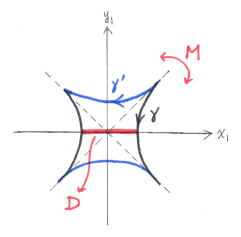
Figure 1: $la$-disk surgery.

Now define

(6) $$\eta_{D}(L):=(L\setminus Orb_{\mathcal{G}}(\gamma))\cup Orb_{\mathcal{G}}(\gamma^{\prime}).$$

Note that $Q=Orb_{\mathcal{G}}(\gamma)$ and $M(Q)=Orb_{\mathcal{G}}(\gamma^{\prime})$ are tangent along their boundary $\partial Q=\partial(M(Q))=M(\partial Q)$, and both tangent to the pair of Lagrangian planes

$$E_{+}:=(\partial_{x_{1}}+\partial_{y_{1}})\wedge(\partial_{x_{2}}+\partial_{y_{2}}),\quad E_{-}:=(-\partial_{x_{1}}+\partial_{y_{1}})\wedge(\partial_{x_{2}}-\partial_{y_{2}}).$$

Notation alert:  The notations $L^{\prime},Q^{\prime},C^{\prime}$ that will be used below have noting to do with the same notations from Section 2.2.

Proposition 2.3.1.

Let $L$ be a Lagrangian surface and $D$ a $la$-disk of $L$. Let $\eta_{D}(L)$ be obtained from $L$ by performing a Lagrangian surgery on $L$ via $D$ as described above. Then $\eta_{D}(L)$ is Lagrangian surface smoothly isotopic to $L$.

Proof.

It is easy to see that $L^{\prime}:=\eta_{D}(L)$ is Lagrangian by Fact 2.2.1. To show that $L^{\prime}$ is smoothly isotopic to $L$, observe that $M=M_{\pi}$ is an element of the $S^{1}$-subgroup $\mathcal{M}:=\{M_{\theta}\mid\theta\in\mathbb{R}/2\pi\mathbb{Z}\}$ of $SO(4)$ whose elements in matrix form with respect to the orthonormal basis $\{\partial_{x_{1}},\partial_{x_{2}},\partial_{y_{1}},\partial_{y_{2}}\}$ are

(7) $$M_{\theta}:=\frac{1}{2}\begin{bmatrix}I+R_{\theta}&I-R_{\theta}\\ I-R_{\theta}&I+R_{\theta}\end{bmatrix}\in SO(4,\mathbb{R}),$$

where

$$R_{\theta}:=\begin{bmatrix}\cos\theta&-\sin\theta\\ \sin\theta&\cos\theta\end{bmatrix}\in SO(2,\mathbb{R}).$$

Both $E_{\pm}$ are preserved by all elements of $\mathcal{M}$: $M_{\theta}$ fixes the plane $E_{+}$ pointwise and rotates the (oriented) plane $E_{-}$ by an angle of $\theta$ radians. Moreover, $\mathcal{M}$ commutes with $\mathcal{G}$. Let

$$Q_{\theta}:=Orb_{\mathcal{G}}(M_{\theta}(\gamma))=M_{\theta}(Orb_{\mathcal{G}}(\gamma)).$$

For $\theta\in[0,\pi]$ define

$$L_{\theta}:=(L\setminus Q)\cup Q_{\theta}$$

Each of $L_{\theta}$ is diffeomorphic to $L$, $L_{0}=L$, $L_{\pi}=L^{\prime}$. Then $L_{\theta}$ is a smooth isotopy between $L$ and $L^{\prime}$. So $L$ and $\eta_{D}(L)=L^{\prime}$ are smoothly isotopic. ∎

Dual $la$-disk surgery  Let $L$, $M$, and $L^{\prime}:=\eta_{D}(L)$ be as above. Let $D^{\prime}:=M(D)$ and $C^{\prime}:=M(C)=\partial D^{\prime}$. Then $C^{\prime}\subset L^{\prime}$ is a vanishing cycle, $D^{\prime}$ is a $la$-disk of $L^{\prime}$ along $C^{\prime}$. Applying the standard model for $\eta_{D}$ one sees that

$$L=\eta_{D^{\prime}}(L^{\prime})=\eta_{D^{\prime}}(\eta_{D}(L)).$$

Remark 2.3.2 (Relation with Polterovich’s Lagrangian surgery).

In [17] Polterovich defined a Lagrangian surgery (for all dimensions) as a way of removing transversal self-intersection points of Lagrangian submanifolds. In the $2$-dimensional case the surgery is done by first cutting off a neighborhood of the nodal point, which is a union of two embedded Lagrangian disks intersecting transversally and in a single point, and then closing up the two boundary circles by gluing a Lagrangian annulus to the complement of the nodal neighborhood along the boundary circles. Compared with our $la$-disk surgery, the nodal neighborhood is precisely $E_{+}\cup E_{-}$, the gluing annulus can be either $Q$ or $M(Q)$, and the resulting Lagrangian surface (with one nodal point removed) is $L$ (resp. $\eta_{D}(L)$) if $Q$ (resp. $M(Q)$) is used for gluing.

Relative polarity.  It is easy to check that $D,D^{\prime}$ are of the same type as $la$-disks of $L,L^{\prime}$ respectively, This can be seen by observing that the isotopy $L_{\theta}$ takes $C=\partial D$ to $C^{\prime}=\partial D^{\prime}$, and induces isomorphisms $H_{1}(L,\mathbb{Z})\cong H_{1}(L^{\prime},\mathbb{Z})$ and $\pi_{1}(L)\cong\pi_{1}(L^{\prime})$. As for polarity, there is a way to compare the polarity of $D,D^{\prime}$ which we describe as follows:

Fix an orientation of the annulus $Q\subset L$. Also fix an orientation of $C\subset Q$. Since $Q$ and $Q^{\prime}:=M(Q)\subset L^{\prime}=\eta_{D}(L)$ are tangent along $\partial Q=\partial Q^{\prime}$, orientation of $Q$ induces an orientation of $Q^{\prime}$ so the two orientations coincides on $T_{\partial Q}Q=T_{\partial Q^{\prime}}Q^{\prime}$. It is easy to see that $C^{\prime}$ also inherit an orientation compatible with that of $C$. Indeed, the orientations of the pair $(Q^{\prime},C^{\prime})$ are obtained by transporting the orientations of $(Q,C)$ via the isotopy $M_{\theta}$.

Let $\nu_{C}\subset T_{C}Q$ be a normal vector field to $C$ in $Q\subset L$ so that the ordered pair $(\nu_{C},\dot{C})$ is a positive basis of $T_{C}Q$. Here $\dot{C}$ denotes the tangent vector field of $C$ with respect to some parameterization compatible with the orientation of $C$. Likewise Let $\nu_{C^{\prime}}\subset T_{C^{\prime}}Q^{\prime}$ be a normal vector field to $C^{\prime}$ in $Q^{\prime}\subset L^{\prime}$ so that the ordered pair $(\nu_{C^{\prime}},\dot{C}^{\prime})$ is a positive basis of $T_{C^{\prime}}Q^{\prime}$. We also denote by $\nu$ the outward normal to $D$ along $C$, by $\nu^{\prime}$ the outward normal to $D^{\prime}$ along $C^{\prime}$. Note that the symplectic normal bundle $N^{\omega}_{C}$ is spanned by $\nu$ and $\nu_{C}$, and similarly $N^{\omega}_{C^{\prime}}$ by $\nu^{\prime}$ and $\nu_{C^{\prime}}$.

Definition 2.3.3.

We say that $D$ and $D^{\prime}$ have the same relative polarity if $\omega(\nu,\nu_{C})$ and $\omega(\nu^{\prime},\nu_{C^{\prime}})$ are of the same $\pm$ sign; and $D$ and $D^{\prime}$ have opposite relative polarities if $\omega(\nu,\nu_{C})$ and $\omega(\nu^{\prime},\nu_{C^{\prime}})$ are of different $\pm$ signs. The notion of relative polarity is independent of the choices of orientations of $Q$ and $C$.

Proposition 2.3.4.

Let $D\subset L$ and $D^{\prime}\subset L^{\prime}=\eta_{D}(L)$ be the corresponding $la$-disks in the $la$-disk surgery. Then $D$ and $D^{\prime}$ have opposite relative polarities.

Proof.

Let $D=\{x_{1}^{2}+x_{2}^{2}\leq(\sqrt{2}-1)^{2}r^{2},\ y_{1}=0=y_{2}\}$ and $Q=Orb_{\mathcal{G}}\gamma$ be as in the standard model. Then $D^{\prime}=\{y_{1}^{2}+y_{2}^{2}\leq(\sqrt{2}-1)^{2}r^{2},\ x_{1}=0=x_{2}\}$, $Q^{\prime}=Orb_{\mathcal{G}}\gamma^{\prime}$. Since $D,D^{\prime},Q,Q^{\prime}$ are $\mathcal{G}$-invariant, we only need to compare $\omega(\nu,\nu_{C})$ at the point $p:=(x_{1}=(\sqrt{2}-1)r,y_{1}=0,x_{2}=0,y_{2}=0)$ and $\omega(\nu^{\prime},\nu_{C^{\prime}})$ at the point $p^{\prime}=M(p)=(x_{1}=0,y_{1}=(\sqrt{2}-1)r,x_{2}=0,y_{2}=0)$. Without loss of generality we may take

$$\nu=\partial_{x_{1}},\quad\nu_{C}=\partial_{y_{1}}\quad\text{ at $p$}.$$

Then by applying $M$, we get

$$\nu^{\prime}=\partial_{y_{1}},\quad\nu_{C^{\prime}}=\partial_{x_{1}}\quad\text{ at $p^{\prime}$}.$$

Since $\omega=\sum_{j=1}^{2}dx_{j}\wedge dy_{j}$,

$$\omega_{p}(\nu,\nu_{C})=1>0,\quad\omega_{p^{\prime}}(\nu^{\prime},\nu_{C^{\prime}})=-1<0.$$

So $D$ and $D^{\prime}$ have opposite relative polarities. ∎

In particular, if $L\subset W$ is a nullhomologous torus in $W$ with $H^{1}(W,\mathbb{Z})=0$, and if $D$ is a stable (resp. unstable) $la$-disk of $L$, then $D^{\prime}$ is a unstable (resp. stable) $la$-disk of $L^{\prime}$.

Example 2.3.5.

Let $L\subset\mathbb{R}^{4}$ be the Chekanov torus and $D$ as defined in Example 2.1.6. Then a $la$-disk surgery along $D$ changes $L$ to $L^{\prime}=\eta_{D}(L)\subset\mathbb{R}^{4}$ a monotone Clifford torus monotone Lagrangian isotopic to the one in Example 2.1.7.

Example 2.3.6.

Consider the cotangent bundle $T^{*}S^{2}$ and regard the zero section $S^{2}=D\cup D^{\prime}$ as a union of two closed Lagrangian disks $D,D^{\prime}$ with $\partial D=C=\partial D^{\prime}$ as the equator. Let $U\subset T^{*}S^{2}$ be a cotangent neighborhood of $D$ and $L^{\prime}\subset U$ be a monotone Clifford torus with $D$ as its unstable $la$-disk, and $D^{\prime}$ as its stable $la$-disk. Then a $la$-disk along $D^{\prime}$ turns $L^{\prime}$ into a monotone torus $L^{\prime\prime}\subset T^{*}S^{2}$ monotone Lagrangian which, up to a scaling by a Liouville vector field, is isotopic to the geodesic torus as defined in Example 2.1.8.

2.4 Relation with generalized Dehn twists

A generalized Dehn twist is defined at the presence of an embedded Lagrangian sphere. Below we describe the model generalized Dehn twist following [19].

Generalized Dehn twist.  Identify a small neighborhood $U_{S}$ of an embedded Lagrangian $2$-sphere $S$ symplectically with a neighborhood $V_{0}$ of the $0$-section of the cotangent bundle $T^{*}S^{2}$, and $S$ identified with $S^{2}$. Use the model

$$T^{*}S^{2}=\{(q,p)\in\mathbb{R}^{3}\times\mathbb{R}^{3}\mid|q|=1\text{ and }\langle q,p\rangle=0\},$$

in which $\omega=\sum_{i}dq_{i}\wedge dp_{i}$. For $x\in\mathbb{R}^{3}\setminus\{0\}$ and $t\in\mathbb{R}$, let $R^{t}(x)\in SO(3)$ be the rotation with axis $x/|x|$ and angle $t$. Define

$$\sigma^{it}(q,p)=(R^{t}(q\times p)q,R^{t}(q\times p)p).$$

Take a function $C^{\infty}(\mathbb{R},\mathbb{R})$ such that $\psi(t)+\psi(-t)=2\pi$ for all $t$, $\psi(t)=0$ for $t\gg 0$, $\psi(t)=\pi$ for small $|t|$, and $\psi(|\xi|)=0\mod 2\pi$ for $\xi\not\in V_{0}$. Then the model generalized Dehn twist $\tau_{S}:W\to W$ is a symplectomorphism with compact support contained in $U_{S}$, and its restriction to $U_{S}\cong V_{0}$ is

$$\tau_{S}(\xi):=\begin{cases}\sigma(e^{i\psi(|\xi|)})(\xi),&\xi\in V_{0}\setminus S^{2},\\ A\xi,&\xi\in S^{2},\end{cases}$$

where $A$ is the antipodal map on $S^{2}$. For $n\in\mathbb{Z}$ the $2n$-th power of $\tau_{S}$ is

$$\tau^{2n}_{S}=\begin{cases}\sigma(e^{2ni\psi(|\xi|)})(\xi),&\xi\in V_{0}\setminus S^{2},\\ \xi,&\xi\in S^{2}.\end{cases}$$

Elliptic $la$-disk.  Let $D$ be an elliptic $la$-disk of a Lagrangian surface $L$ with boundary $C=\partial D\subset L$ which bounds an embedded disk $\Delta\subset L$. Identify a neighborhood $U$ of $\Delta$ symplectically with an open domain $V\subset T^{*}\mathbb{R}^{2}$ so that under this identification

$$\Delta =\{x_{1}^{2}+x_{2}^{2}\leq 1,\ y_{1}=0=y_{2}\},$$

$$U =\{x_{1}^{2}+x_{2}^{2}<1+\epsilon_{1},\ y_{1}^{2}+y_{2}^{2}<\epsilon_{2}^{2}\},$$

where $(y_{1},y_{2})$ are the corresponding fiber coordinates for $T^{*}\Delta$, and $D\cap U$ is one of the following two sets according to the polarity of $D$:

• $A_{+}:=\{x^{2}=1,\ x_{1}y_{2}=x_{2}y_{1},\ x_{1}y_{1}\geq 0\}\cap U$,

• $A_{-}:=\{x^{2}=1,\ x_{1}y_{2}=x_{2}y_{1},\ x_{1}y_{1}\leq 0\}\cap U$.

Remark 2.4.1.

Note that $(A_{+}\setminus C)\sqcup(A_{-}\setminus C)$ is isomorphic to the quotient $\mathbb{R}$-bundle $(TC)^{\omega}/T_{C}\Delta$ with the zero section $C$ deleted. The polarization of $((TC)^{\omega}/T_{C}\Delta)\setminus C$ by assigning $\pm$ signs to each of the two connected components as defined above is independent of the choice of a coordinate system for $\Delta$.

Remark 2.4.2.

The above sign assignment is even independent of the choice of $\Delta\subset L$ with $\partial\Delta=C$. Indeed, suppose there is another embedded disk $\hat{\Delta}\subset L$ with $\partial\hat{\Delta}=C$, and this happens precisely when $L$ is a sphere. Parameterize $\hat{\Delta}$ with coordinates $(\hat{x}_{1},\hat{x}_{2})\in\mathbb{R}^{2}$ so that $\hat{\Delta}=\{(\hat{x}_{1})^{2}+(\hat{x}_{2})^{2}\leq 1\}$. Let $(\hat{y}_{1},\hat{y}_{2})$ be the corresponding fiber coordinates for $T^{*}\hat{\Delta}$. We may assume that along $C=\partial D=\partial\hat{\Delta}$

$$x_{1}=-\hat{x}_{1},\quad x_{2}=\hat{x}_{2}.$$

Let $\pi:T^{*}L\to L$ denote the canonical projection. For $p\in\pi^{-1}(C)$, its $(x,y)$ coordinates and $(\hat{x},\hat{y})$ coordinates are related by the equations

$$x_{1}=-\hat{x}_{1},\ x_{2}=\hat{x}_{2},\ y_{1}=-\hat{y}_{1},\ y_{2}=\hat{y}_{2}.$$

The equation $x_{1}y_{2}=x_{2}y_{1}$ is then equivalent to $\hat{x}_{1}\hat{y}_{2}=\hat{x}_{2}\hat{y}_{1}$. In addition $x_{1}y_{1}=\hat{x}_{1}\hat{y}_{1}$, so the sign assignment is independent of the choice of $\Delta\subset L$.

We proceed to analyze the surgery $\eta_{D}$ applied to $L$.

Proposition 2.4.3.

Let $L\subset(W,\omega)$ be an embedded oriented Lagrangian surface. Let $D$ be an elliptic $la$-disk to $L$ with $\partial D=C$. Let $\Delta\subset L$ be an embedded disk with $\partial\Delta=C$. Then the union $D\cup\Delta$ associates an embedded Lagrangian sphere $S$, $S$ is unique up to Hamiltonian isotopy, such that $S$ intersects with $L$ transversally and in a single point. Let $\nu$, $\nu^{\prime}$ denote respectively the outward normal of $D$ and $\Delta$ along $C$. Let $\eta_{D}(L)$ denote the Lagrangian surface obtained by applying to $L$ the Lagrangian surgery on $L$ via $D$. We have the following conclusions:

1. Assume that $\omega(\nu,\nu^{\prime})>0$, then $\eta_{D}(L)$ is Hamiltonian isotopic to $\tau^{2}_{S}(L)$, where $\tau_{S}$ is the positive generalized double Dehn twist along $S$.

2. Assume that $\omega(\nu,\nu^{\prime})<0$, then $\eta_{D}(L)$ is Hamiltonian isotopic to $\tau^{-2}_{S}(L)$, the squared negative generalized double Dehn twist along $S$.

Moreover, $\eta_{D}(L)\pitchfork S$ and $\eta_{D}(L)\cap S=L\cap S$.

Proof.

Case 1:  $\omega(\nu,\nu^{\prime})>0$.  In this case we have $D\cap U=A_{+}$. We can construct an embedded Lagrangian sphere $S$ which intersects transversally with $L$ and in a single point. The construction is done by properly smoothing out the corner curve $C$ of the union $D\cup\Delta$ as follows.

Let $f:[-1,1]\subset\mathbb{R}_{x_{1}}\to\mathbb{R}$ be a continuous function satisfying the following conditions:

• $f(-x_{1})=-f(x_{1})$, $0\leq|f|\leq\epsilon_{2}/2$,

• $f$ is smooth on $(-1,0)\cup(0,1)$, $f^{\prime}(x_{1})>0$ on $(-1,0)\cup(0,1)$,

• $\lim_{x_{1}\to 0}f^{\prime}(x_{1})=\infty$, $\lim_{x_{1}\to-1^{+}}f^{\prime}(x_{1})=\lim_{x_{1}\to 1^{-}}f^{\prime}(x_{1})=\infty$.

Let $\gamma_{f}\subset\mathbb{R}^{2}_{x_{1}y_{1}}$ denote the graph of $f$, and

$$S:=D_{1}\cup\Delta_{f},$$

where

• $D_{1}:=D-\{y_{1}^{2}+y_{2}^{2}\leq|f(\pm 1)|\}$, and

• $\Delta_{f}:=Orb_{\mathcal{G}}(\gamma_{f})$.

Then $S$ is an embedded Lagrangian sphere, and the conditions on $f$ ensure that

$$S\cap L=\{0\}\in\Delta\quad\text{and}\quad S\pitchfork L.$$

Note that $0\neq[L]\in H_{2}(W,\mathbb{Z})$. We can choose coordinates $(x_{1},x_{2})$ on $\Delta$ so that $dx_{1}\wedge dx_{2}$ is an area form.

We can choose $f$ so that the projection of $S\cap U$ to the $(y_{1},y_{2})$-coordinate plane gives a coordinate system of $S\cap U$. One sees that $\{-\partial_{x_{1}},-\partial_{x_{2}}\}$ is the corresponding dual basis for $T^{*}_{0}S$.

Recall $\tau^{2}_{S}$ the square of the positive generalized Dehn twist along $S$. We may assume that $\tau^{2}_{S}$ is supported in a cotangent neighborhood of $S$, and $\tau^{2}_{S}=id$ near $S$.

Since on $U$ the sets $S\cap U$, $D\cap U$, $\Delta$ and the symplectic form $\omega|_{U}$ are invariant under the Hamiltonian $\mathcal{G}$-action, we may assume that $\tau^{2}_{S}$ is also $S^{1}$-invariant when restricted to the intersection of a cotangent neighborhood of $S$ with $U$. Thus we can describe the effect of $\tau^{2}_{S}$ on $L$ by looking at the corresponding picture in the $(x_{1},y_{1})$-coordinate plane $E$.

We may assume that $\text{Supp}(\tau^{2}_{S})\cap L=\{0<\delta_{1}\leq x_{1}^{2}+x_{2}^{2}\leq\delta_{2},y_{1}=0=y_{2}\}$. Here $\text{Supp}(\tau^{2}_{S})$ denotes the support of $\tau^{2}_{S}$. Now for each $\theta\in[0,2\pi]$, $\tau^{2}_{S}$ sends the oriented line segment $\ell_{\theta}(s)=(x_{1}=s\cos\theta,x_{2}=s\sin\theta,y_{1}=0,y_{2}=0)\subset\text{Supp}(\tau^{2}_{S})\cap L$, $\delta_{1}\leq|s|\leq\delta_{2}$, to a curve which projects to the simple geodesic circle in $S$ passing through the north pole $0\in\Delta$ and is oriented by the vector $\dfrac{d\ell}{ds}(\delta_{1})$. Note that $\tau^{2}_{S}$ is independent of the orientation of $S$.

With the $S_{1}$-symmetry associated with $\mathcal{G}$ we can depict the $E$-slice of $R:=\tau^{2}_{S}(L)\cap U$ as the bold black curve in the right picture of Figure 2. Let us denote by $R_{E}$ the $E$-slice of $R$.

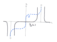
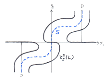
Figure 2: $\eta_{D}(L)$ and $\tau_{S}^{2}(L)$.

Since $S=\Delta_{f}\cup D_{1}$ and we treat $0\in\Delta_{f}$ as the north pole of $S$, we can view $D_{1}$ as the southern hemisphere of $S$. Let $p_{s}\subset D_{1}$ denote the south pole of $S$. we can also parameterize $D$ so that $p_{s}$ is the origin of the 2-disk $D$. Note that the Lagrangian disk surgery $\eta_{D}$ replaces a collar neighborhood $U_{C}$ of $C=\partial D\subset L$ by a Lagrangian annulus symplectomorphic to the total space in $T^{*}D\cong TD$ of of oriented geodesics with a fixed constant speed in $D$ (with respect to the standard Euclidean metric) passing through $p_{s}\in D$. The annulus $U_{C}\subset L$ can be symplectically identified with a neighborhood of the zero section of a 1-dimensional subbundle $V$ of $T^{*}_{C}L$ over $C$. Then $U_{C}$ has a fibration over $C$ with fiber $\ell_{x}\subset V_{x}$ over $x\in C$, and up to a Hamiltonian isotopy with $\partial U$ fixed, $\eta_{D}(\ell_{x})\subset T^{*}_{C}D\cong T_{C}D$ is a curve that projects to an oriented geodesic line in $D$, passing through $p_{s}$, and with orientation uniquely specified by $x\in C$. In particular, $\ell_{x}$ and $\ell_{-x}$ correspond to the same geodesic line but with different orientations. Note that since $C\subset L$ is homologically trivial, up to Hamiltonian isotopy the resulting Lagrangian surface $\eta_{D}(L)$ does not depend on the precise surgery size of $\eta_{D}$. Thus we may assume that

• $\Gamma:=\eta_{D}(L)\cap U=Orb_{\mathcal{G}}(\Gamma_{E})$ is the orbit of $\Gamma_{E}$ (the bold black curve in the left picture of Figure 2) under the Hamiltonian $\mathcal{G}$-action, $\Gamma_{E}$ is invariant under the $180^{\circ}$-rotation of $E=\partial_{x_{1}}\wedge\partial_{y_{1}}$ centered at $0\in\Delta$, and $\partial\Gamma_{E}=\partial R_{E}$;

On $E$ there is a Hamiltonian isotopy $\phi_{t}$ supported in a compact set in $U\cap E$, $\phi_{0}=id$, $\phi_{1}(R)=\Gamma$, such that $\phi_{t}$ commutes with the said $180^{\circ}$-rotation and $\phi_{t}$ fixes $\partial\Gamma$ for all $t$. Observe that $\phi_{t}$ can be extended to a Hamiltonian isotopy on $W$, compactly supported in $U$, commuting with the Hamiltonian $S^{1}$-action (so that all $R_{t}:=\phi_{t}(R)$ are $S^{1}$-invariant), such that $\phi_{1}(R)=\Gamma$ and $\phi_{t}=id$ near $\partial R$ for all $t$. We obtain that $\eta_{D}(L)$ is Hamiltonian isotopic to $\tau^{2}_{S}(L)$. Hence up to Hamiltonian isotopy $\eta_{D}=\tau^{2}_{S}$ as surgeries on $L$.

Case 2:   $\omega(\nu,\nu^{\prime})<0$.  The discussion goes almost parallel to Case 1, with several changes:

1. $D\cap U=A_{-}$.

2. For the construction of $S$ replace $f$ by $-f$.

3. $\tau^{2}_{S}$ is replaced by $\tau^{-2}_{S}$ the square of the negative generalized Dehn twist along $S$.

4. The conclusion is that $\eta_{D}(L)$ and $\tau^{-2}_{S}(L)$ are Hamiltonian isotopic. Hence $\eta_{D}|_{L}\cong\tau^{-2}_{S}|_{L}$.

∎

Remark 2.4.4.

When $L=S^{2}$ is a Lagrangian sphere, the attaching circle $C=\partial D$ bounds two distinct disks $\Delta$ and $\hat{\Delta}$ in $L=\Delta\cup-\hat{\Delta}$. Let $S,\hat{S}$ be the Lagrangian sphere associated to $D\cup-\Delta$ and $D\cup\hat{\Delta}$ respectively. Then up to a choice of orientation, the homology classes of $S$ and $\hat{S}$ differ by the homology class of $L$. Nevertheless $\tau^{2}_{\hat{S}}(L)$ and $\tau^{2}_{S}(L)$ are Hamiltonian isotopic.

The polarity of an elliptic $la$-disk can be described in terms of the $\pm$-sign of $\omega(\nu,\nu^{\prime})$ as defined in Proposition 2.4.3:

Definition 2.4.5 (Polarity of an elliptic $la$-disk).

We say that an elliptic $la$-disk $D$ of $L$ is positive if it satisfies $\omega(\nu,\nu^{\prime})>0$ as in Proposition 2.4.3(i), negative if it satisfies $\omega(\nu,\nu^{\prime})<0$ instead.

Lemma 2.4.6 (Elliptic pair).

Let $D$ be an elliptic $la$-disk of $L$ with $C:=\partial D$ bounds an embedded disk $\Delta\subset L$. Then there is another elliptic $la$-disk $D^{\prime}$ of $L$ with $\partial D^{\prime}=C$ such that

1. $D^{\prime}$ and $D$ have opposite polarity;

2. $\eta_{D^{\prime}}(L)$ is Hamiltonian isotopic to $\tau^{-2}_{S}(L)$, where $\tau_{S}$ is the generalized double Dehn twist associated to $D$.

Proof.

Assume first that $D$ is positive. The negative elliptic $la$-disk $D^{\prime}$ with $\partial D^{\prime}=C$ can the obtained from $D$ as indicated in Figure 3.

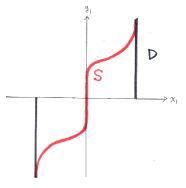
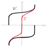
Figure 3: Positive $D$ and negative $D^{\prime}$.

It is easy to see that the Lagrangian sphere associated to $D^{\prime}$ as depicted in Figure 3 is Hamiltonian isotopic to the Lagrangian sphere $S$ associated to $D$. That $\eta_{D^{\prime}}(L)$ and $\tau^{-2}_{S}(L)$ being Hamiltonian isotopic follows from Proposition 2.4.3(ii).

The negative $D$ case can be verified in a similar way. ∎

Corollary 2.4.7 (Infinite order).

Let $D,D^{\prime},L$ be as defined in Lemma 2.4.6. Assume that $D$ is positive and $D^{\prime}$ is negative. Then for each $n\in\mathbb{N}$, $\eta^{n}_{D}(L)$ is defined and is Hamiltonian isotopic to $\tau^{2n}_{S}(L)$. Similarly, $\eta_{D^{\prime}}^{n}(L)$ is defined and is Hamiltonian isotopic to $\tau^{-2n}_{S}(L)$, $n\in\mathbb{N}$.

Proof.

Let $L^{1}:=\eta_{D}(L)$. Up to Hamiltonian isotopy $L^{1}=\tau^{2}_{S}(L)$ as depicted in the right-hand picture of Figure 2. There one observes that $\tau^{2}_{S}(L)$ contains a smaller disk $\Delta_{1}\subset\Delta$, and $C_{1}:=\partial\Delta_{1}$ is also the boundary of a positive elliptic $la$-disk $D_{1}$ of $\tau^{2}_{S}(L)$ such that $D_{1}=D$ outside $U$ (recall $\Delta$ and $U$ from the proof of Proposition 2.4.3). We can define $L^{2}:=\eta^{2}_{D}(L):=\eta_{D_{1}}\circ\eta_{D}(L)=\eta_{D_{1}}(L^{1})$. Since $\eta_{D_{1}}(L^{1})$ is Hamiltonian isotopic to $\tau^{2}_{S}(L^{1})$, we have that $L^{2}:=\eta^{2}_{D}(L)$ is Hamiltonian isotopic to $\tau^{2}_{S}(L^{1})=\tau^{4}_{S}(L)$. Repeat the process with $L^{1}$ replaced by $L^{2}$ and so on so forth we get infinitely many smoothly isotopic Lagrangian surfaces $L^{n}:=\eta_{D}^{n}(L)=\eta_{D_{n-1}}(L^{n-1})$, $D_{0}=D$, $L^{0}=L$, $n\in\mathbb{N}$, and $L^{n}$ is Hamiltonian isotopic to $\tau^{2n}_{S}(L)$.

The $\eta_{D^{\prime}}$ case can be proved by exactly the same type of argument. This completes the proof. ∎

2.5 Properties of $la$-disk surgery

Below we discuss the effect of $la$-disk surgery on the minimal Maslov number, the Liouville class, and the monotonicity of Lagrangian surfaces (see [15] for detailed definitions). For simplicity we assume that $c_{1}(W)=0$ and $\pi_{1}(W)=0$. We also assume that $L$ is orientable. Then the Maslov class $\mu_{L}$ of $L$ is an element of $H^{1}(L,\mathbb{Z})$ and the Liouville class $\alpha_{L}$ is in $H^{1}(L,\mathbb{R})$. If $\mu_{L}\neq 0$ then we define the minimal Maslov number of $L$ to be

$$m_{L}:=\min\{\mu_{L}(\tau)\mid\tau\in H_{1}(L,\mathbb{Z}),\ \mu(\tau)>0\},$$

and we set $m_{L}=0$ if $\mu_{L}=0$. We say that $L$ is monotone if there is a constant $c>0$ such that

$$\alpha_{L}=c\cdot\mu_{L}.$$

Let $L^{\prime}=\eta_{D}(L)$ be obtained from $L$ by a $la$-disk surgery along a $la$-disk $D$ of $L$. If $L=S^{2}$ then both $\mu_{L}$ and $\alpha_{L}$ vanish, so are $\mu_{L^{\prime}}$ and $\alpha_{L^{\prime}}$. We may assume that the genus of $L$ is $g>0$. Then the intersection pairing

$$H_{1}(L;\mathbb{Z})\times H_{1}(L;\mathbb{Z})\to\mathbb{Z},\quad(\sigma,\eta)\to\sigma\cdot\eta,$$

is unimodular. For $\sigma\in H_{1}(L;\mathbb{Z})$ we denote

$$\sigma^{\perp}:=\{\zeta\in H_{1}(L;\mathbb{Z})\mid\sigma\cdot\zeta=0\}.$$

Proposition 2.5.1.

Let $L,L^{\prime}=\eta_{D}(L)$ be as in Proposition 2.3.1. Assume in addition that $c_{1}(W)=0$ and $\pi_{1}(W)=0$. Then $L,L^{\prime}$ have the same minimal Maslov number. If in addition that $L$ is orientable and monotone, then $L^{\prime}$ is monotone iff the kernel of the Liouville class $\alpha_{L}:H_{1}(L;\mathbb{Z})\to\mathbb{R}$ satisfies

$$\ker(\alpha_{L})\subset[C]^{\perp}.$$

In particular, if $L$ is a monotone Lagrangian torus then so is $L^{\prime}$. Moreover, if $[C]=0\in H_{1}(L,\mathbb{Z})$, then $L^{\prime}$ is monotone and $\alpha_{L^{\prime}}$ is isomorphic to $\alpha_{L}$ as cohomology classes.

Proof.

Let $C:=\partial D$. Let $U_{C}\subset L$ be a collar neighborhood of $C\subset L$ such that $L\setminus U_{C}\subset L^{\prime}$. If $\sigma\in H_{1}(L,\mathbb{Z})$ satisfies $\sigma\cdot[C]=0$ then $\sigma=[\beta]$ for some curve $\beta\subset L$ disjoint from $U_{C}$. Hence $\beta\subset L^{\prime}$ and $\mu_{L^{\prime}}([\beta])=\mu_{L}([\beta])$. Similarly we have $\alpha_{L^{\prime}}([\beta])=\alpha_{L}([\beta])$.

Now let $\sigma$ be a generator of the quotient group of $H_{1}(L,\mathbb{Z})$ by $[C]^{\perp}$. We may assume that $\sigma\cdot[C]=1$. Represent $2\sigma$ by two disjoint embedded curves $\beta_{\pm}\subset L$ such that each of $\beta_{\pm}$ intersects with $C$ transversally at a single point, and $\gamma_{\pm}:=\beta_{\pm}\cap U_{D}$ is contained in the $x_{1}y_{1}$-coordinate plane so that $\gamma_{+}=\gamma$ as defined in (3), $\gamma_{-}\subset\{x_{1}<0\}$, and $\gamma_{+}\cup\gamma_{-}$ is invariant under the $180^{\circ}$-rotation of the $x_{1}y_{1}$-plane with $(0,0)\in\mathbb{R}^{2}_{x_{1},y_{1}}$ as the center point.

Since $\pi_{1}(W)=0$, there exist smooth maps $\psi_{\pm}:(D^{2},\partial D^{2})\to(W,\beta_{\pm})$ of disks with boundary circles mapped to $\beta_{\pm}$ respectively. Let $D_{\pm}:=\psi_{\pm}(D^{2})$. We may assume that $B_{\pm}:=D_{\pm}\cap U_{D}$ is contained in the $x_{1}y_{1}$-plane such that $B_{+}\subset\{x_{1}>0\}$, $B_{-}\subset\{x_{1}<0\}$, and $B_{+}\cup B_{-}$ is also invariant under the $180^{\circ}$-rotation described above. We may also assume that $\psi_{\pm}$ is a smooth embedding when restricted to $V_{\pm}:=\psi^{-1}_{\pm}(B_{\pm})$.

Recall the anti-symplectic rotation $M$ as defined in (4). Let $\gamma^{\prime}_{\pm}:=M(\gamma_{\pm}$). Let $\beta^{\prime}$ denote the closure of the union of $(\beta_{\pm}\setminus\gamma_{\pm})\cup\gamma^{\prime}_{\pm}$. Then $\beta^{\prime}\subset L^{\prime}$ is a simple closed curve representing a class $\sigma^{\prime}\in H_{1}(L^{\prime},\mathbb{Z})$ satisfying $\sigma^{\prime}\cdot[C^{\prime}]=2$. Let $Z\subset\mathbb{R}^{2}_{x_{1}y_{1}}$ denote the closed region bounded by $\gamma_{\pm}$ and $\gamma^{\prime}_{\pm}$. Let $D^{\prime}:=D_{-}\cup Z\cup D_{+}$, then $D^{\prime}$ is a disk with $\partial D^{\prime}=\beta^{\prime}$.

Pick a symplectic trivialization $\Psi_{\pm}$ of $\psi_{\pm}^{*}TW$ so that $\Psi_{\pm}|_{V_{\pm}}$ is the standard symplectic trivialization of $TW$ on $B_{\pm}$. It is easy to see that $D^{\prime}$ is the image of a smooth map $\psi^{\prime}:(D^{2},\partial D^{2})\to(W,\gamma^{\prime})$ such that $\psi^{\prime}$ is an embedding when restricted to $V^{\prime}:=\psi^{-1}(B)$ where $B=B_{-}\cup Z\cup B_{+}$. Choose a symplectic trivialization $\Psi^{\prime}$ of $\psi^{\prime*}TW$ so that $\Psi^{\prime}|_{V^{\prime}}$ is just the standard symplectic trivialization of $TW$ on $B$ and $\Psi^{\prime}=\Psi_{\pm}$ when restricted to the preimages of $D\setminus B_{\pm}$ respectively. Now the comparison of $\mu_{L}(\beta_{-}\cup\beta_{+})$ and $\mu_{L^{\prime}}(\beta^{\prime})$ is reduced to the calculation of the Maslov angles of $\gamma_{-}\cup\gamma_{+}$ and $\gamma^{\prime}_{-}\cup\gamma^{\prime}_{+}$. An easy computation shows the two angles are equal. Thus we have

$$\mu_{L^{\prime}}(\sigma^{\prime})=\mu_{L}(2\sigma).$$

Note that $\sigma$ is primitive and $\sigma^{\prime}$ is twice of a primitive class. We conclude that $\mu_{L}$ and $\mu_{L^{\prime}}$ have the same minimal Maslov number.

Also we have

$$\alpha_{L^{\prime}}(\sigma^{\prime})=2\cdot\alpha_{L}(\sigma)+\int_{Z}\omega,$$

here the orientation of $Z$ is determined by the orientation of its boundary $\partial Z=\gamma^{\prime}_{+}\cup(-\gamma_{-})\cup\gamma^{\prime}_{-}\cup(-\gamma_{+})$. Here $-\gamma_{-}$ denotes $\gamma_{-}$ but with its orientation reversed, and $\bar{\gamma}_{+}$ is defined in a similar way. So $\int_{Z}\omega>0$ if $\partial Z$ is oriented counterclockwise, $\int_{Z}\omega<0$ if otherwise.

Thus if $L$ is monotone then $L^{\prime}$ is monotone iff $\ker(\alpha_{L})\subset[C]^{\perp}$. In particular, this condition is met when $[C]=0\in H_{1}(L,\mathbb{Z})$. On the other hand, if $L$ is a torus (and monotone) then the condition $\ker(\alpha_{L})\subset[C]^{\perp}$ is automatically satisfied, even though $[C]\neq 0$. So the monotonicity of a Lagrangian torus is preserved under $la$-disk surgery. ∎

3 Lagrangian Grassmannian

3.1 Decomposition and group action

In this section we review Lagrangian Grassmannian of a $4$-dimensional symplectic vector space $V$. Since $V$ is linearly isomorphic to the standard symplectic $4$-space $(\mathbb{R}^{4},\omega=\sum_{j=1}^{2}dx_{j}\wedge y_{j})$, we will identify $V$ with $(\mathbb{R}^{4},\omega)$ without further notice. Denote by $\Lambda^{+}$ the space of all oriented Lagrangian planes in $V$.

Factorization of $\Lambda^{+}$.  Let $J:V\to V$ be a complex structure compatible with $\omega$, i.e., $J$ is a linear map with $J^{2}=-Id$, and the composition $\omega\circ(Id\times J):V\times V\to\mathbb{R}$ is positive definite and symmetric. The pair $(\omega,J)$ associate a unique inner product $g:=\omega\circ(Id\times J)$ on $V$, and the structure group is reduced to the unitary group $U(2)$ associated to $(\omega,J)$. For notational convenience, we will often represent an oriented 2-dimensional subspace $E\subset V$ as a $2$-vector $E=v_{1}\wedge v_{2}$ formed by an oriented basis $\{v_{1},v_{2}\}$ of $E$. We will also denote by $E^{\perp}$ the oriented 2-dimensional subspace in $V$ $g$-orthogonal to $E$ such that the orientation of $E\wedge E^{\perp}$ is that of their ambient symplectic vector space $V=\mathbb{R}^{4}$.

Fix a unitary basis $(u,v)$. There is a unique $g$-orthogonal complex structure $K^{\prime}$ on $V$ such that $u\wedge v$ is $K^{\prime}$-complex. i.e., $v=K^{\prime}u$. Let $K^{\prime\prime}:=JK^{\prime}$. We have $K^{\prime}K^{\prime\prime}=J$, $K^{\prime\prime}J=K^{\prime}$. The triple $(J,K^{\prime},K^{\prime\prime})$ generate an $S^{2}$-family of $g$-orthogonal complex structures

$$J_{a,b,c}:=aJ+bK^{\prime}+cK^{\prime\prime},\quad a^{2}+b^{2}+c^{2}=1.$$

Let

$$K_{t}:=\cos tK^{\prime}+\sin tK^{\prime\prime},\quad t\in\mathbb{R}/2\pi\mathbb{Z}.$$

Note that $K_{t}$-complex planes are Lagrangian planes. We have the following decomposition of $\Lambda^{+}$:

(8) $$\Lambda^{+}=\bigsqcup_{t\in\mathbb{R}/2\pi\mathbb{Z}}\mathbb{P}(K_{t}),$$

where $\mathbb{P}(K_{t})\cong\mathbb{C}P^{1}\cong S^{2}$ is the Grassmannian of $K_{t}$-complex 2-dimensional subspaces of $V$. We also denote by $\mathbb{P}(J)$ the Grassmannian of $J$-complex planes. We call (8) a $J$-decomposition of $\Lambda^{+}$.

Remark 3.1.1.

A different choice of a unitary basis $(u,v)$ amounts to changing the parameter $t$ in (8) by adding a constant. In addition, the space of $\omega$-compatible complex structures on $V$ is contractible, hence any two $J$-decompositions of $\Lambda^{+}$ are homotopic.

For example, if $J$ is the standard complex structure on $\mathbb{C}^{2}\cong\mathbb{R}^{4}$ defined by

$$J\partial_{x_{j}}=\partial_{y_{j}},\quad j=1,2,$$

then $g$ is the Euclidean metric on $\mathbb{R}^{4}$. Pick the unitary basis

$$u:=\partial_{x_{1}},\quad v=\partial_{x_{2}},$$

then $K^{\prime},K^{\prime\prime}$ are defined by

(9) $$K^{\prime}\partial_{x_{1}}=\partial_{x_{2}}, \quad K^{\prime}\partial_{y_{1}}=-\partial_{y_{2}}$$

(10) $$K^{\prime\prime}\partial_{x_{1}}=\partial_{y_{2}}, \quad K^{\prime\prime}\partial_{y_{1}}=-\partial_{x_{2}}.$$

Although the choice of $u,v$ play no big role in the decomposition of $\Lambda^{+}$ as in (8), the oriented Lagrangian plane $u\wedge v$ associates a unique oriented $S^{1}$-subgroup of $SU(2)$ as well as a unique oriented $S^{1}$-family of $J$-complex planes, leading to a parameterization of $\Lambda^{+}$ which will be described below. First review some basic facts about the $U(2)$-action on $\Lambda^{+}$.

Action of $U(2)$ on $\Lambda^{+}$.  The unitary group $U(2)$ associated to $(\omega,J)$ acts on $\Lambda^{+}$. Let $\mathcal{C}\subset U(2)$ denote the subgroup of centralizers of $U(2)$. With respect to any unitary basis (e.g., $\{u,v\}$), the matrix representative of $\mathcal{C}$ is

(11) $$\mathcal{C}=\Big{\{}c_{t}=\begin{pmatrix}e^{it}&0\\ 0&e^{it}\end{pmatrix}\mid t\in\mathbb{R}/2\pi\mathbb{Z}\Big{\}}.$$

$\mathcal{C}$ acts on $\Lambda^{+}$ by rotations:

(12) $$c_{\tau}(\mathbb{P}(K_{t}))=\mathbb{P}(K_{t+2\tau}),$$

with $c_{\pi}=-Id$ acts trivially on $\Lambda^{+}$. Note that $\mathcal{C}$ acts trivially on $\mathbb{P}(J)$, $c_{t}$ rotates the total space of each element $E\in\mathbb{P}(J)$ by an angle of $t$-radians with respect to the orientation of $E$.

On the other hand, the special unitary subgroup $SU(2)\subset U(2)$ acts on each of $\mathbb{P}(K_{t})$ as well as on $\mathbb{P}(J)$ by rotations, with its centralizer subgroup $\{\pm Id\}$ acts as the isotropy subgroup of the action. Indeed, the action of $SU(2)/\{\pm Id\}$ on $\mathbb{P}(J)$ and on each of $\mathbb{P}(K_{t})$ can be identified with the canonical action of $SO(3)$ on the unit 2-sphere $S^{2}\subset\mathbb{R}^{3}$. Also $SU(2)$ commutes with all $J_{a,b,c}$, and in particular $K_{t}$ for $t\in\mathbb{R}/2\pi\mathbb{Z}$.

As a homogeneous space $\mathbb{P}(K_{t})\cong SU(2)/S^{1}\cong S^{2}$ is endowed with an $SU(2)$-equivariant metric unique up to scaling. We take the one with which the area of $\mathbb{P}(K^{\prime})$ is $\pi$, then $\mathbb{P}(K_{t})$ is a standard sphere with diameter 1. We also endow $\mathbb{P}(J_{a,b,c})$ with the same kind of metric for $(a,b,c)\in S^{2}$.

An $S^{1}$-subgroup $\mathcal{H}\subset SU(2)$ acts on each of $\mathbb{P}(J_{a,b,c})$ by standard rotations. There is a unique $\mathcal{H}$-orbit in $\mathbb{P}(J_{a,b,c})$ which is a great circle with respect the $SU(2)$-equivariant metric. We call this special orbit the geodesic $\mathcal{H}$-orbit in $\mathbb{P}(J_{a,b,c})$.

3.2 Intersection of complex and Lagrangian planes

Definition 3.2.1 (Complex locus).

Let $Z\subset V\cong\mathbb{R}^{4}$ be an oriented two dimensional subspace. The complex locus of $Z$ is defined to be

$$\mathcal{E}_{Z}:=\{E\in\mathbb{P}(J)\mid E\cap Z\neq\{0\}\}.$$

Proposition 3.2.2.

Let $(u,v)$ be a positive orthonormal basis of $Z$. Then

$$\mathcal{E}_{Z}=\{E_{\theta}:=u_{\theta}\wedge Ju_{\theta}\mid\theta\in\mathbb{R}/\pi\mathbb{Z}\},$$

where $u_{\theta}:=u\cos\theta+v\sin\theta$. So $\mathcal{E}_{Z}$ is a (possibly degenerated) circle in $\mathbb{P}(J)$. And $\mathcal{E}_{Z}$ consists of a single point iff $Z\in\mathbb{P}(J)$ or $Z\in\mathbb{P}(-J)$.

It is easy to see that $\mathcal{E}_{Z}=\{Z\}$ if $Z$ is $J$-complex, and $\mathcal{E}_{Z}=\{-Z\}$ if $Z$ is $(-J)$-complex.

In general $Z$ is $J_{a,b,c}$-complex for some unique $(a,b,c)\in S^{2}$. $SU(2)$ acts on the $J_{a,b,c}$-complex Grassmannian $\mathbb{P}(J_{a,b,c})\cong S^{2}$ by rotations with $\{\pm Id\}$ as the isotropy subgroup. There is a unique $S^{1}$-subgroup $\mathcal{H}\subset SU(2)$ fixing the pair $Z,Z^{\perp}\in\mathbb{P}(J_{a,b,c})$. $\mathcal{H}$ acts as rotations on the total spaces of $Z$ and $Z^{\perp}$ respectively. We can orient $\mathcal{H}=\{h_{s}\mid s\in\mathbb{R}/2\pi\mathbb{Z}\}$ with $h_{0}=Id$ so that $h_{s}$ rotates $Z$ by an angle of $s$-radians, whilst it rotates $Z^{\perp}$ by an angle of $(-s)$-radians, with respect to the orientation associated with the complex structure $J_{a,b,c}$. By definition, $\mathcal{H}$ also acts on $\mathcal{E}_{Z}$ by rotations. Combining with the proposition above we have the following lemma.

Lemma 3.2.3.

The complex locus $\mathcal{E}_{Z}$ is a connected $\mathcal{H}$-orbit and hence a latitude in $\mathbb{P}(J)$ with respect to the fixed points of $\mathcal{H}$ in $\mathbb{P}(J)$, where $\mathcal{H}\subset SU(2)$ is the stabilizer subgroup of $Z$.

Proposition 3.2.4.

The two complex loci $\mathcal{E}_{Z}$ and $\mathcal{E}_{Z^{\perp}}$ are either disjoint or equal. Moreover, $\mathcal{E}_{Z}=\mathcal{E}_{Z^{\perp}}$ iff $Z$ is Lagrangian.

Proof.

Observe that $Z$ and $Z^{\perp}$ have the same stabilizer subgroup $\mathcal{H}\subset SU(2)$, hence both $\mathcal{E}_{Z}$ and $\mathcal{E}_{Z^{\perp}}$ are connected $\mathcal{H}$-orbit in $\mathbb{P}(J)$. So $\mathcal{E}_{Z}\cap\mathcal{E}_{Z^{\perp}}=\emptyset$ if $\mathcal{E}_{Z}\neq\mathcal{E}_{Z^{\perp}}$.

To verify the second statement we may assume that $Z$ is neither $J$-complex nor $(-J)$-complex without loss of generality. Write $Z=u\wedge J_{a,b,c}u$ with $u$ unitary and $a\neq 0$, Then

$$\mathcal{E}_{Z}=\{E_{\theta}:=(u\cos\theta+J_{a,b,c}u\sin\theta)\wedge J(u\cos\theta+J_{a,b,c}u\sin\theta)\mid\theta\in\mathbb{R}/\mathbb{Z}\}.$$

Assume that $\mathcal{E}_{Z}=\mathcal{E}_{Z^{\perp}}$. Then for any $\theta\in\mathbb{R}/\pi\mathbb{Z}$, we have $\dim E_{\theta}\cap Z=1=\dim E_{\theta}\cap Z^{\perp}$, and $(E_{\theta}\cap Z)\perp Z^{\perp}$, $(E_{\theta}\cap Z^{\perp})\perp Z$ since $Z\perp Z^{\perp}$. This implies that $E_{\theta}\cap Z^{\perp}$ is spanned by $J(u\cos\theta+J_{a,b,c}u\sin\theta)$. Same conclusion holds if we replace $\theta$ by $\theta^{\perp}:=\theta+\frac{\pi}{2}$. Thus we must have $Z^{\perp}=-JZ$, hence $Z$ is Lagrangian.

Conversely, assume that $Z$ is Lagrangian, then $J_{a,b,c}=K_{t}$ for some $t\in\mathbb{R}/2\pi\mathbb{Z}$. Since the centralizer subgroup $\mathcal{C}\subset U(2)$ commutes with $SU(2)$ and $c_{\frac{-t}{2}}(Z)\in\mathbb{P}(K^{\prime})$, we may assume that $Z\in\mathbb{P}(K^{\prime})$ without loss of generality. Then we can write $Z=u\wedge K^{\prime}u$, and $Z^{\perp}=K^{\prime\prime}u\wedge Ju=JK^{\prime}u\wedge Ju$. That $\mathcal{E}_{Z}=\mathcal{E}_{Z^{\perp}}$ can be easily verified by direct computation. This completes the proof. ∎

Proposition 3.2.5.

The complex locus $\mathcal{E}_{Z}$ is a great circle in $\mathbb{P}(J)$ iff $Z$ is Lagrangian.

Proof.

Let $\mathcal{H}\subset SU(2)$ be the stabilizer subgroup of $Z$, and $\mathcal{N}(\mathcal{H})$ the group of normalizers of $\mathcal{H}$ in $SU(2)$. It is well known that $\mathcal{N}(\mathcal{H})/\mathcal{H}\cong\mathbb{Z}_{2}$. Let $\rho\in\mathcal{N}(\mathcal{H})$ be an element representing the nontrivial element of $\mathcal{N}(\mathcal{H})/\mathcal{H}$. Then $\rho^{2}=Id$, $\rho h_{s}\rho^{-1}=h_{-s}=h^{-1}_{s}$ for any $h_{s}\in\mathcal{H}$. So $\rho$ preserves the orbit space of $\mathcal{H}$ but reverses the orientation of $\mathcal{H}$. Since $\rho$ maps the stabilizer subgroup $\mathcal{H}_{Z}=\mathcal{H}$ of $Z$ to the stabilizer subgroup $\mathcal{H}_{Z^{\perp}}=\mathcal{H}^{-1}$ of $Z^{\perp}$ we have $\rho(\mathcal{E}_{Z})=\mathcal{E}_{Z^{\perp}}$.

By a direct computation one can show that $\rho$ acts on $\mathbb{P}(J)$ as a $180^{\circ}$ rotation with respect to a pair of antipodal points lying on the geodesic $\mathcal{H}$-orbit which is a great circle in $\mathbb{P}(J)$. In particular, the geodesic $\mathcal{H}$-orbit is the unique $\mathcal{H}$-orbit preserved by $\rho$. So $\mathcal{E}_{Z}$ is a great circle in $\mathbb{P}(J)$ iff $\rho(\mathcal{E}_{Z})=\mathcal{E}_{Z}$. Since $\rho(\mathcal{E}_{Z})=\mathcal{E}_{Z^{\perp}}$ we conclude that $\mathcal{E}_{Z}$ is a great circle in $\mathbb{P}(J)$ iff $Z$ is Lagrangian by Proposition 3.2.4. ∎

Corollary 3.2.6.

Given $Z,Z^{\prime}\in\Lambda^{+}$, then

$$\mathcal{E}_{Z}\cap\mathcal{E}_{Z^{\prime}}=\begin{cases}\mathcal{E}_{Z}&\text{ if $Z^{\prime}\in Orb_{\mathcal{C}}(\{Z,Z^{\perp}\})\subset\Lambda^{+}$},\\ \text{ 2 points}&\text{ else}.\end{cases}$$

Definition 3.2.7 (Lagrangian locus).

For every $J$-complex plane $E\subset\mathbb{P}(J)$ we define the Lagrangian locus $\Lambda^{+}_{E,t}$ of $E$ in $\mathbb{P}(K_{t})$ to be the set of all $K_{t}$-complex complex planes which intersects nontrivially with $E$, i.e.,

$$\Lambda^{+}_{E,t}:=\{F\in\mathbb{P}(K_{t})\mid\dim F\cap E=1\}.$$

We also define the total Lagrangian locus $\Lambda^{+}_{E}$ of $E$ to be

$$\Lambda^{+}_{E}:=\cup_{t}\Lambda^{+}_{E,t}.$$

Proposition 3.2.8.

1. Let $E\in\mathbb{P}(J)$, then for each $t$, $\Lambda^{+}_{E,t}\cong S^{1}$ is a great circle in $\mathbb{P}(K_{t})$, and $\mathcal{C}$ acts on $\Lambda^{+}_{E}$:

   $$c_{\frac{t^{\prime}}{2}}(\Lambda^{+}_{E,t})=\Lambda^{+}_{E,t+t^{\prime}}.$$

2. For $E,E^{\prime}\in\mathbb{P}(J)$ with $E\neq E^{\prime}$,

   $$\Lambda^{+}_{E,t}\cap\Lambda^{+}_{E^{\prime},t}=\begin{cases}\text{ 2 points}&\text{ if $E^{\prime}\neq E^{\perp}$}\\ \Lambda^{+}_{E,t}=\Lambda^{+}_{E^{\prime},t}&\text{ if $E^{\prime}=E^{\perp}$}.\end{cases}$$

Proof.

For $t\in\mathbb{R}/2\pi\mathbb{Z}$ let $\omega_{t}:=g\circ(K_{t}\oplus Id)$ denote the nondegenerate anti-symmetric bilinear form (i.e. a linear symplectic form) on $V=\mathbb{R}^{4}$ with respect to the complex structure $K_{t}$. Elements of $\mathbb{P}(J)$ are $\omega_{t}$-Lagrangian for all $t$. Then (i) and (ii) follow easily from Propositions 3.2.4 and 3.2.5, and the action of $\mathcal{C}$ on $\Lambda^{+}$ as discussed in Section 3.1. ∎

Lemma 3.2.9.

Given $E_{0}\in\mathbb{P}(J)$ and an $S^{1}$-subgroup $\mathcal{G}$ of $SU(2)$ we denote by $\mathcal{E}:=Orb_{\mathcal{G}}(E_{0})$ the $\mathcal{G}$-orbit of $E_{0}$ in $\mathbb{P}(J)$. Then for any $t\in\mathbb{R}/2\pi\mathbb{Z}$,

$$\mathbb{P}(K_{t})=\underset{E\in\mathcal{E}}{\bigcup}\Lambda^{+}_{E,t}\quad\Longleftrightarrow\quad\text{ $\mathcal{E}$ is a great circle}.$$

Proof.

For any $Z\in\mathbb{P}(K_{t})$ we have

$$\begin{split}Z\in\underset{E\in\mathcal{E}}{\bigcup}\Lambda^{+}_{E,t}\ &\Longleftrightarrow\text{ $\dim(Z\cap E)=1$ for some $E\in\mathcal{E}$}\\ &\Longleftrightarrow\text{ $E\in\mathcal{E}_{Z}$ for some $E\in\mathcal{E}$}.\end{split}$$

The map

$$\mathbb{P}(K_{t})\to\{\text{ great circles in $\mathbb{P}(J)$}\}$$

by sending $Z\in\mathbb{P}(K_{t})$ to $\mathcal{E}_{Z}$ is a 2:1 surjective map. If $\mathcal{E}$ is a great circle, then it will intersects with every great circle in $\mathbb{P}(J)$ at least twice, which implies that $\mathbb{P}(K_{t})=\underset{E\in\mathcal{E}}{\bigcup}\Lambda^{+}_{E,t}$. On the other hand, if $\mathcal{E}$ is not a great circle, then it is contained in some open hemisphere $D$ of $\mathbb{P}(J)$ and hence misses at least one (in fact, infinitely may) great circle: the boundary $\partial D$ of $D$. Since $\partial D=\mathcal{E}_{Z}$ for some $Z\in\mathbb{P}(K_{t})$ we conclude that $\mathbb{P}(K_{t})\supsetneqq\underset{E\in\mathcal{E}}{\bigcup}\Lambda^{+}_{E,t}$. This completes the proof. ∎

Applying Proposition 3.2.5 we have the following result.

Corollary 3.2.10.

For any $Z\in\mathbb{P}(K_{t})$, we have

$$\mathbb{P}(K_{t})=\underset{E\in\mathcal{E}_{Z}}{\bigcup}\Lambda^{+}_{E,t},\quad\text{and}$$

$$\Lambda^{+}=\underset{t\in\mathbb{R}/2\pi\mathbb{Z}}{\bigcup}(\underset{E\in\mathcal{E}_{Z}}{\cup}\Lambda^{+}_{E,t}).$$

Remark 3.2.11.

For $E\in\mathbb{P}(J)$ and $a\neq 0$ one can also define the intersection locus of $E$ in $\mathbb{P}(J_{a,b,c})$ to be $\mathbb{P}(J_{a,b,c})_{E}:=\{Z\in\mathbb{P}(J_{a,b,c})\mid\dim Z\cap E>0\}$. Then $\mathbb{P}(J_{a,b,c})_{E}$ is a connected orbit of the stabilizer subgroup $\mathcal{H}_{E}\subset SU(2)$ of $E$, but it is not a great circle in in $\mathbb{P}(J_{a,b,c})$. This follows from the observation that $E$ is not Lagrangian with respect to the symplectic form $\omega_{a,b,c}:=g\circ(J_{a,b,c}\oplus Id)$ associated to $J_{a,b,c}$, provided that $a\neq 0$. Likewise, in contrast to the Lagrangian case, for any $S^{1}$-subgroup $\mathcal{H}\subset SU(2)$ and any $E_{0}\in\mathbb{P}(J)$, the union of the intersection loci $\cup_{E\in Orb_{\mathcal{H}}(E_{0})}\mathbb{P}(J_{a,b,c})_{E}$ will never cover $\mathbb{P}(J_{a,b,c})$ if $a\neq 0$, even if $Orb_{\mathcal{H}}(E_{0})$ is a great circle in $\mathbb{P}(J)$. This covering property of intersection loci set Lagrangian planes apart from the totally real ones, and will enable us to device a new invariant for Lagrangian surfaces with stronger rigidity than some of the classical ones.

3.3 Spherical coordinates adapted to $(u,v)$

Fix a unitary basis $(u,v)$ and let $Z:=u\wedge v\in\mathbb{P}(K^{\prime})$. Let $\mathcal{G}\subset SU(2)$ denote the stabilizer subgroup of $Z$. The matrix representation of $\mathcal{G}$ with respect to the unitary basis $u,v$ is

$$\mathcal{G}=\Big{\{}g_{\theta}=\begin{pmatrix}\cos\theta&-\sin\theta\\ \sin\theta&\cos\theta\end{pmatrix}\mid\theta\in\mathbb{R}/2\pi\mathbb{Z}\Big{\}}.$$

Here the parameter $\theta$ is chosen so that $\textsf{g}_{\theta}$ rotates the $K^{\prime}$-complex plane $Z$ by an angle of $\theta$-radians, with respect to the $K^{\prime}$-complex orientation of $Z$. Simultaneously $g_{\theta}$ rotates $Z^{\perp}$ by an angle of $(-\theta)$-radians, also with respect to the $K^{\prime}$-complex orientation of $Z^{\perp}$.

Recall the complex locus $\mathcal{E}_{Z}$. We parameterize $\mathcal{E}_{Z}$ by $\theta\in\mathbb{R}/\pi\mathbb{Z}$:

$$\mathcal{E}_{Z}=\{E_{\theta}\in\mathbb{P}(J)\mid E_{\theta}=u_{\theta}\wedge Ju_{\theta}\},$$

where $u_{\theta}:=u\cos\theta+v\sin\theta$.

For each $\theta\in\mathbb{R}/\pi\mathbb{Z}$, we denote by $\lambda_{\theta}$ the Lagrangian locus $\Lambda^{+}_{E_{\theta},0}$ of $E_{\theta}$ in $\mathbb{P}(K^{\prime})=\mathbb{P}(K_{0})$:

$$\lambda_{\theta}:=\{\xi\in\mathbb{P}(K^{\prime})\mid\dim(\xi\cap E_{\theta})=1\}.$$

Each of $\lambda_{\theta}$ is a great circle in $\mathbb{P}(K^{\prime})$ passing through $Z$ and $Z^{\perp}$. Note that (recall $\theta^{\perp}=\theta+\frac{\pi}{2}$)

$$\lambda_{\theta^{\perp}}=\lambda_{\theta},\quad\theta\in\mathbb{R}/\pi\mathbb{Z}.$$

For each $\theta$, we choose $u_{\theta}$ as the basis for $E_{\theta}$. Denote $\xi\in\mathbb{P}(K^{\prime})$ as

$$\xi=\lambda_{\theta}(s)\quad\theta,s\in\mathbb{R}/\pi\mathbb{Z}$$

$$\text{if }\ \xi\in\lambda_{\theta}\ \ \text{and}\ \ \xi\cap E_{\theta}=\text{Span}\{u_{\theta}\cos s+Ju_{\theta}\sin s\}.$$

We have

1. $\lambda_{\theta^{\perp}}(s)=\lambda_{\theta}(\pi-s)=\lambda_{\theta}(-s)=(\lambda_{\theta}(\frac{\pi}{2}-s))^{\perp}$ for $\theta,s\in\mathbb{R}/\pi\mathbb{Z}$, and

2. $Z=\lambda_{\theta}(0)$, $Z^{\perp}=\lambda_{\theta}(\frac{\pi}{2})$ for $\theta\in\mathbb{R}/\pi\mathbb{Z}$.

The parameter $s$ not only corresponds to the angle of rotation of the intersection subspace $\text{Span}\{u_{\theta,s}\}$ in $E_{\theta}$, but also parameterize the orbit space of $\mathcal{G}$ in $\mathbb{P}(K^{\prime})$ if $s$ is restricted to either $[0,\frac{\pi}{2}]$ or $[\frac{\pi}{2},\pi]$. Then

$$\Phi_{+}:\mathbb{R}/\pi\mathbb{Z}\times[0,\pi/2]\to\mathbb{P}(K^{\prime}),\quad\Phi_{+}(\theta,s):=\lambda_{\theta}(s)$$

is a modified spherical coordinate system for $\mathbb{P}(K^{\prime})\cong S^{2}$. To compare $\Phi_{+}$ with the homogeneous coordinates of $\mathbb{P}(K^{\prime})$ we may take $u,v$ to be

$$u=\partial_{x_{1}},\quad v=\partial_{x_{2}}$$

without loss of generality. Let $x=x_{1}+ix_{2}$ and $y=y_{1}-iy_{2}$ be the $K^{\prime}$-complex coordinates. Then $\mathbb{P}(K^{\prime})$ is parameterized by the homogeneous coordinates $[x:y]$:

$$\mathbb{P}(K^{\prime})=\{[x:y]\mid(x,y)\in\mathbb{C}^{2}\setminus\{(0,0)\}\},$$

$$[x:y]=[x^{\prime}:y^{\prime}]\Leftrightarrow(x^{\prime},y^{\prime})=(\lambda x,\lambda y)\text{ for some $\lambda\in\mathbb{C}^{*}$}.$$

In particular the points

$$\xi_{0}:=[1:0]\ \text{ and }\ \xi_{\infty}:=[0:1]$$

represent $Z=\partial_{x_{1}}\wedge\partial_{x_{2}}$ and $Z^{\perp}=\partial_{y_{1}}\wedge(-\partial_{y_{2}})$ respectively. The tangent plane $T_{\xi}\mathbb{P}(K^{\prime})$ can be identified with the total space of $\xi^{\perp}$. A direct computation yields the identity

$$\lambda_{\theta}(s)=[e^{i\theta}\cos s:e^{-i\theta}\sin s],\quad\theta,s\in\mathbb{R}/\pi\mathbb{Z}.$$

Moreover, the induced orientation on $\mathbb{P}(K^{\prime})$ via $\Phi_{+}$ coincides with the orientation on $\mathbb{P}(K^{\prime})$ inherited from its $K^{\prime}$-complex structure.

Note that the other parameterization

$$\Phi_{-}:\mathbb{R}/\pi\mathbb{Z}\times[\frac{\pi}{2},\pi]\to\mathbb{P}(K^{\prime}),$$

$$\Phi_{-}(\theta,s):=\lambda_{\theta}(s),$$

induces the opposite orientation on $\mathbb{P}(K^{\prime})$.

The action of $c_{t}\in\mathcal{C}$ on $\Lambda^{+}$ carries the spherical trivialization $\Phi_{+}$ on $\mathbb{P}(K^{\prime})=\mathbb{P}(K_{0})$ over $\mathbb{P}(K_{2t})$. Observe that $\mathcal{C}$ commutes with $\mathcal{G}$. In fact, $\mathcal{C}$ and $\mathcal{G}$ together generate a maximal torus $\mathcal{T}_{\mathcal{G}}$ of $U(2)$. Accordingly we obtain an $\mathcal{T}_{\mathcal{G}}$-equivariant trivialization

$$\tilde{\Phi}:\mathbb{R}/2\pi\mathbb{Z}\times\mathbb{R}/\pi\mathbb{Z}\times[0,\frac{\pi}{2}]\to\Lambda^{+}$$

(13) $$\tilde{\Phi}(t,\theta,s):=c_{\frac{t}{2}}(\lambda_{\theta}(s)).$$

With $\tilde{\Phi}$ we can identify $\Lambda^{+}$ with $S^{1}\times S^{2}$, so that $\{t\}\times S^{2}\cong\mathbb{P}(K_{t})$, and the projection $S^{1}\times S^{2}\to S^{2}$ corresponds to the central projection

$$\pi^{\prime} :\Lambda^{+}\to\mathbb{P}(K^{\prime}),$$

(14) $$\pi^{\prime}(\xi) :=c_{-\frac{t}{2}}(\xi)\quad\text{ if $\xi\in\mathbb{P}(K_{t})$}.$$

Remark 3.3.1.

The parameter $\theta\in\mathbb{R}/\pi\mathbb{Z}$ , which parameterizes complex planes $E_{\theta}$, increases clockwise around $\xi_{0}$ and counterclockwise around $\xi_{\infty}$.

Orientation of $\lambda_{\theta}$.  Observe that $\lambda_{\theta}=\lambda_{\theta^{\perp}}$ comes with two different orientations. Denote by $\lambda_{\theta}^{+}$ as $\lambda_{\theta}$ with the orientation induced $E_{\theta}$, and by $\lambda_{\theta}^{-}$ as $\lambda_{\theta}$ but with the orientation induced by $-E_{\theta}$. We have

$$\lambda_{\theta}^{+}=\lambda_{\theta^{\perp}}^{-},\quad\lambda_{\theta}^{-}=\lambda_{\theta^{\perp}}^{+}.$$

Relative $E_{\theta}$-phase.  As we trace out $\lambda^{+}_{\theta}$ once, the intersection subspace $\lambda^{+}(s)\cap E_{\theta}$ rotates in $E_{\theta}$ by an angle of $\pi$-radians, whilst $\lambda^{+}_{\theta}\cap E_{\theta^{\perp}}$ rotates in $E_{\theta^{\perp}}$ by an angle of $(-\pi)$-radians, we call the former minus the latter, denoted as $(\Delta\varphi)_{\lambda^{+}_{\theta}}$, the relative phase of $E_{\theta}$ along $\lambda^{+}_{\theta}$, which is

(15) $$(\Delta\varphi)_{\lambda^{+}_{\theta}}=2\pi.$$

An alternative description of the orientations of $\lambda_{\theta}$ is in order: The complement $\mathbb{P}(K^{\prime})\setminus\lambda_{\theta}$ consists of two disjoint open disks:

$$\mathbb{P}(K^{\prime})\setminus\lambda_{\theta}=D_{\theta}\sqcup D_{\theta^{\perp}},$$

where

(16) $$D_{\theta} :=\{\xi\in\mathbb{P}(K^{\prime})\mid\xi\pitchfork E_{\theta},\ \xi\wedge E_{\theta}>0\}$$

$$=\{\lambda_{\theta^{\prime}}(s)\in\mathbb{P}(K^{\prime})\mid\theta-\frac{\pi}{2}<\theta^{\prime}<\theta\mod\pi,\ 0<s<\frac{\pi}{2}\},$$

(17) $$D_{\theta^{\perp}} :=\{\xi\in\mathbb{P}(K^{\prime})\mid\xi\pitchfork E_{\theta^{\perp}},\ \xi\wedge E_{\theta^{\perp}}>0\}$$

$$=\{\lambda_{\theta^{\prime}}(s)\in\mathbb{P}(K^{\prime})\mid\theta<\theta^{\prime}<\theta^{\perp}\mod\pi,\ 0<s<\frac{\pi}{2}\}.$$

Note that for $\xi\in\mathbb{P}(K^{\prime})$

$$\xi\wedge E_{\theta}>0\ \Longleftrightarrow\ \xi\wedge E_{\theta^{\perp}}<0.$$

Then

$$\lambda_{\theta}^{+}=\lambda_{\theta^{\perp}}^{-}=\partial D_{\theta},\quad\lambda_{\theta^{\perp}}^{+}=\lambda_{\theta}^{-}=\partial D_{\theta^{\perp}}$$

as oriented boundaries. Similar conclusions hold straightforwardly for complex loci $\lambda^{t}_{\theta}:=\Lambda^{+}_{E_{\theta},t}\in\mathbb{P}(K_{t})$ by applying the rotation $c_{\frac{t}{2}}$.

3.4 Maps into $\mathbb{P}(K^{\prime})$

Recall that $\xi_{0}:=u\wedge v\in\mathbb{P}(K^{\prime})$ denotes the oriented Lagrangian plane which corresponds to the south pole $[1:0]$ of $\mathbb{P}(K^{\prime})=\{[e^{i\theta}\cos s:e^{-i\theta}\sin s]\mid\theta\in\mathbb{R}/\pi\mathbb{Z},\ s\in[0,\frac{\pi}{2}]\}$.

A suitable neighborhood $U_{\xi_{0}}$ of $\xi_{0}$ in $\Lambda^{+}$ can be identified with the space of symmetric $2\times 2$ matrices

$$S=\begin{pmatrix}a+c&b\\ b&-a+c\end{pmatrix},\quad a,b,c\in\mathbb{R},$$

so that with respect to the orthonormal basis $\{u,v,Ju,Jv\}$ the column vectors of the $4\times 2$ matrix $\begin{pmatrix}I\\ S\end{pmatrix}$ form a basis of the corresponding Lagrangian plane $\xi\in U_{\xi_{0}}$. In particular, $\xi\in\mathbb{P}(K^{\prime})$ iff the trace of $S$ is $\text{tr}S:=2c=0$. In this case $[1:a-ib]$ is the homogeneous coordinate of $\xi\in\mathbb{P}(K^{\prime})$, with

$$\tan 2\theta=\frac{b}{a},\quad\tan s=\sqrt{a^{2}+b^{2}}.$$

Indeed the map

$$[e^{i\theta}\cos s:e^{-i\theta}\sin s]\to(a=\cos 2\theta\tan s,-b=-\sin 2\theta\tan s)$$

is the stereographic projection map of $\mathbb{P}(K^{\prime})\setminus\{[0:1]\}$ from its north pole $\xi_{\infty}=[0:1]$ onto $\mathbb{R}^{2}$.

Let $L$ be an oriented surface and $g_{L}:L\to\Lambda^{+}$ a smooth map. Composing $g_{L}$ with the projection $\pi^{\prime}:\Lambda^{+}\to\mathbb{P}(K^{\prime})$ we get

$$g^{\prime}_{L}:=\pi^{\prime}\circ g_{L}:L\to\mathbb{P}(K^{\prime}).$$

Given $q_{0}\in L$ and assume that $g^{\prime}_{L}(q_{0})=\xi_{\infty}$ for the moment. Let $U\subset\mathbb{R}^{2}$ be a coordinate neighborhood of $q_{0}$ with coordinates $(x_{1},x_{2})$ such that $g^{\prime}_{L}(U)\subset\mathbb{P}(K^{\prime})\setminus\{\xi_{\infty}\}$. Then near $q_{0}$ the map $g^{\prime}_{L}$ can be expressed as

$$g^{\prime}_{L}(x_{1},x_{2})=(a(x_{1},x_{2}),-b(x_{1},x_{2})).$$

Then by a direct computation we find for $q\in U$

$$b(q)\cos 2\theta-a(q)\sin 2\theta\begin{cases}>0&\text{ iff $g^{\prime}_{L}(q)\in D_{\theta}$},\\ =0&\text{ iff $g^{\prime}_{L}(q)\in\lambda_{\theta}$},\\ <0&\text{ iff $g^{\prime}_{L}(q)\in D_{\theta^{\perp}}$}.\end{cases}$$

We denote $a_{i}:=\frac{\partial a}{\partial x_{i}}$ and similarly $b_{j}:=\frac{\partial b}{\partial x_{j}}$. The differential $dg^{\prime}_{L}$ can be expresses as a matrix

$$dg^{\prime}_{L}(q)=\begin{pmatrix}a_{1}(q)&a_{2}(q)\\ -b_{1}(q)&-b_{2}(q)\end{pmatrix}.$$

Then $q$ is a singular point of $q^{\prime}_{L}$ iff $\det dg^{\prime}_{L}(q)=0$, i.e., if the gradient vectors $\nabla a$ and $\nabla b$ are linearly dependent at $q$.

We will use the following notations:

$$L^{+} :=\{q\in L\mid\det dg^{\prime}_{L}(q)>0\}$$

$$L^{o} :=\{q\in L\mid\det dg^{\prime}_{L}(q)=0\}$$

$$L^{-} :=\{q\in L\mid\det dg^{\prime}_{L}(q)<0\}$$

$$V_{\theta} :=(g^{\prime}_{L})^{-1}(D_{\theta})$$

$$\Gamma_{\theta} :=(g^{\prime}_{L})^{-1}(\lambda_{\theta})=(g^{\prime}_{L})^{-1}(\partial D_{\theta})$$

Recall that $\Gamma_{\theta}=\Gamma_{\theta^{\perp}}$. Generically each of $\Gamma_{\theta}\subset L$ is a $1$-dimensional skeleton together with a finite number of isolated points. Since

$$\Gamma_{\theta}=\{q\in L\mid\dim E_{\theta}\cap g^{\prime}_{L}(q)=1\}=\{q\in L\mid\dim E_{\theta}\cap g_{L}(q)=1\}$$

we call $\Gamma_{\theta}$ the $E_{\theta}$-locus of $g^{\prime}_{L}$. Note that

$$(g^{\prime}_{L})^{-1}(\{\xi_{0},\xi_{\infty}\})\subset\Gamma_{\theta},\quad\forall\theta\in\mathbb{R}/\pi\mathbb{Z},$$

and for $\theta,\theta^{\prime}\in[0,\frac{\pi}{2})$ with $\theta\neq\theta^{\prime}$,

$$\Gamma_{\theta}\cap\Gamma_{\theta^{\prime}}=(g^{\prime}_{L})^{-1}(\{\xi_{0},\xi_{\infty}\}).$$

Curves in $L^{o}$.  Generically the set $L^{o}$ of singular points of $g^{\prime}_{L}$ is a $1$-dimensional skeleton, the union of a finite number of immersed closed curves and a finite number of isolated points.

Let $\sigma\subset L^{o}$ be a connected immersed closed curve with a finite number of self-intersection points. Recall that if $g^{\prime}_{L}(\sigma)$ misses the point $\xi_{\infty}$ and $dg^{\prime}_{L}|_{q}\neq 0$ at $q\in\sigma$, then the kernel of $dg^{\prime}_{L}|_{q}$ is tangent to level sets $\{a=a(q)\}$ and $\{b=b(q)\}$ at $q$.

Definition 3.4.1 (Sign-changing).

We say $\sigma$ is sign-changing if the determinant $\det dg^{\prime}_{L}$ changes its $\pm$-signs at $\sigma$, i.e., if $\sigma$ is contained in the closure of $L^{+}$ as well as the closure of $L^{-}$.

The sign-changing property is persistent under a small perturbation of $g^{\prime}_{L}$. If $\sigma$ is not sign-changing then it may disappear or split into a pair of sign-changing curves under a small perturbation $g^{\prime}_{L}$.

Definition 3.4.2 (Ordinary folding curve).

We say that a sign-changing curve $\sigma$ is an ordinary folding curve if its tangent $\dot{\sigma}(q)\not\in\ker(dg^{\prime}_{L})$ for all but a finite number of points $q\in\sigma$.

The image $g^{\prime}_{L}(\sigma)$ is $1$-dimensional if $\sigma$ is an ordinary folding curve. On the other hand, there may exist a curve in $L^{o}$ whose image in $\mathbb{P}(K^{\prime})$ is a point.

Definition 3.4.3 ($p$-curve).

Let $\xi$ be a singular value of $g^{\prime}_{L}$. Then a 1-dimensional connected component $\gamma\subset L^{o}$ of $(g^{\prime}_{L})^{-1}(\xi)$ is called a $p$-curve.

Let $\xi$ be a singular value of $g^{\prime}_{L}$. Suppose that $(g^{\prime}_{L})^{-1}(\xi)$ contains some 1-dimensional connected components. Let $\gamma$ be one of the connected components. Assume for the moment that $g^{\prime}_{L}(\gamma)=\xi\neq\xi_{\infty}$. Then by composing with the stereographic projection from $\mathbb{P}(K^{\prime})\setminus\{\xi_{\infty}\}$ to $\mathbb{R}^{2}$, we can easily see that $\gamma$ is a common level curve to both $a$ and $b$, i.e., $\gamma\subset a^{-1}(a_{0})$ and $\gamma\subset b^{-1}(b_{0})$ for some $a_{0},b_{0}\in\mathbb{R}$. In general $a_{0},b_{0}$ are not regular values of $a$ and $b$ respectively. Generically along $a^{-1}(a_{0})$ the gradient $\nabla a$ of $a$ vanishes only at a finite set $S_{a}\subset a^{-1}(a_{0})$. Similarly, $\nabla b\neq 0$ along $b^{-1}(b_{0})$ except at a finite set $S_{b}\subset b^{-1}(b_{0})$. Since $\gamma$ is of dimension one, $S_{a}\cap S_{b}\cap\gamma$ is empty generically. This means that along $\gamma$, the normal bundle $N_{\gamma/L}$ of $\gamma$ is fiberwise spanned by $\nabla a$ and $\nabla b$, which implies that $\gamma$ is smoothly embedded, and along $\gamma$ the differential $dg^{\prime}_{L}$ is of rank one and $\ker(dg^{\prime}_{L})$ is spanned by $\dot{\gamma}$ the tangent of $\gamma$. This also applies to the case when $g^{\prime}_{L}(\gamma)=\xi_{\infty}$. Note that it is possible that $\gamma$ is still embedded even though $\nabla a$ and $\nabla b$ together need not span $N_{\gamma/L}$ along $\gamma$.

Terminology alert:   Since $p$-curves of $g^{\prime}_{L}$ are (smoothly) embedded for generic $g^{\prime}_{L}$, from now on all $p$-curves are assumed to be embedded unless otherwise mentioned. A $p$-curve which is not embedded will be called a singular $p$-curve. The same abuse of language also applied to folding $p$-curves and crossing $p$-curves which will be defined below.

Folding v.s. crossing. Let $\gamma$ be a $p$-curve and $U=U_{\gamma}\subset L$ be a small tubular neighborhood of $\gamma$ so that $\xi=g^{\prime}_{L}(\gamma)\not\in g^{\prime}_{L}(U\setminus\gamma)$. We parametrize $U$ as $\mathbb{R}/2\pi\mathbb{Z}\times(-\epsilon,\epsilon)$ with coordinates $(x_{1},x_{2})$ so that $\gamma=\{x_{2}=0\}$. Let $U^{+}:=U\cap\{x_{2}>0\}$ and $U^{-}:=U\cap\{x_{2}<0\}$. Denote coordinate curves $\gamma_{s}:=\{x_{2}=s\}$, $\ell_{\theta}:=\{x_{1}=\theta\}$. Also let $\ell^{+}_{\theta}:=\ell_{\theta}\cap\{x_{2}\geq 0\}$, $\ell^{-}_{\theta}:=\ell_{\theta}\cap\{x_{2}\leq 0\}$.

Let $D=D_{\xi}\subset\mathbb{P}(K^{\prime})$ be a neighborhood of $\xi$ diffeomorphic to an open disk. Identify $D$ with a disk of radius $\delta>0$ with center $\xi$, and let $(\rho,t)\in[0,\delta)\times\mathbb{R}/2\pi\mathbb{Z}$ be polar coordinates on $D$ with $\xi=\{\rho=0\}$. Identify $\gamma_{s}$ as $\mathbb{R}/2\pi\mathbb{Z}$, then $t|_{\gamma_{s}}$, $0<s<\epsilon$, is a smooth family of maps which extends continuously over $s=0$. Indeed $t(x_{1},s)$ is the angle (oriented counterclockwise) from the polar axis of $\xi$ to the secant line connecting $\xi$ and $g^{\prime}_{L}(x_{1},s)$ and pointing away from $\xi$, then $t(x_{1},0)$ is defined to be the angle from the polar axis to the oriented tangent line of the image curve $g^{\prime}_{L}(\ell^{+}_{x_{1}})$ at $\xi$, also pointing away from $\xi$. Put together we get a continuous map $t^{+}:U^{+}\cup\gamma\to S^{1}$ which is smooth on $U^{+}$. The same holds true for the $s\leq 0$ case. We denote the corresponding map as $t^{-}:U^{-}\cup\gamma\to S^{1}$. Since $g^{\prime}_{L}(\ell^{+}_{x_{1}})$ and $g^{\prime}_{L}(\ell^{-}_{x_{1}})$ have the same unoriented tangent line at $\xi$ and $g^{\prime}_{L}(U^{\pm})$ are disjoint from $\xi$, by comparing the oriented tangent lines of $g^{\prime}_{L}(\ell_{x_{1}}^{\pm})$ at $\xi$ and by continuity of $t^{\pm}$ on $x_{1}$ exactly one of the followings will be satisfied:

(F).

$t^{-}(x_{1},0)=t^{+}(x_{1},0)\mod 2\pi$,

(C).

$t^{-}(x_{1},0)=t^{+}(x_{1},0)+\pi\mod 2\pi$.

In Case (F) the image $g^{\prime}_{L}(\ell_{x_{1}})$ has $\xi$ as its cusp point since the oriented tangent lines of $g^{\prime}_{L}(\ell^{\pm}_{x_{1}})$ at $\xi$ point to the same direction. Thus the images of all $\ell_{x_{1}}$ ”fold back” at $\xi$. Also in this case, $t^{-}$ and $t^{+}$ together form a continuous function on $U$, or equivalently, the composition of $g^{\prime}_{L}$ with the coordinate function $t$ of $D_{\xi}$ is a continuous function on $U$. Note that here $\rho\geq 0$ also lifts to a smooth function on $U$.

In Case (C) the oriented tangent line for the image of $\ell_{x_{1}}$ at $\xi$ is defined for each $x_{1}$, meaning that the image curves of $\ell_{x_{1}}$ all ”cross” the point $\xi$ at $x_{2}=0$ as $x_{2}$ increases from negative to positive. The two functions $t^{-}$ and $t^{+}$ do not match at $x_{2}=0$. Hence $t$ does not lift to a continuous function on $U$. This however can be remedied at the expense of allowing $\rho$ to be negative, namely instead of $(\rho,t)$ we consider the extended polar coordinates $(\tilde{\rho},\tilde{t})\in(-\delta,\delta)\times\mathbb{R}/2\pi\mathbb{Z}$ with the equivalence relation $(\tilde{\rho},\tilde{t}+\pi)\sim(-\tilde{\rho},\tilde{t})$. Then both $\tilde{\rho}$ and $\tilde{t}$ lift to functions continuous on $U$ and smooth when $x_{2}\neq 0$:

$$(\tilde{\rho},\tilde{t})=\begin{cases}(\rho,t^{+})&\text{ when $x_{2}\geq 0$},\\ (-\rho,t^{-}-\pi)&\text{ when $x_{2}<0$}.\end{cases}$$

Definition 3.4.4 (Crossing v.s. folding).

Let We say that a $p$-curve $\gamma$ is a folding $p$-curve if (F) holds for $\gamma$; a crossing $p$-curve if (C) holds instead.

Below we give a different description about the folding/crossing dichotomy of $p$-curves. Let $\gamma$ be a $p$-curve, $\xi:=g^{\prime}_{L}(\gamma)$, $D_{\xi}\subset\mathbb{P}(K^{\prime})$ an open disk with polar coordinates $(\rho,t)\in[0,\delta)\times\mathbb{R}/2\pi\mathbb{Z}$ centered at $\xi$. Then $g^{\prime}_{L}(L^{o})$ intersects transversally with level sets of $\rho$ on $D_{\xi}\setminus\{\xi\}$ provided $\delta>0$ is small enough. This implies that there exist a tubular neighborhood $U=U_{\gamma}\subset L$ missing all $p$-curves except for $\gamma$, and coordinates $(x_{1},x_{2})\in\mathbb{R}/2\pi\mathbb{Z}\times(-\epsilon,\epsilon)$ for $U$ so that

(c1).

$\rho$ depends only on $x_{2}$, $\frac{\partial\rho}{\partial x_{2}}\neq 0$ on $U\setminus\gamma$,

(c2).

$\rho^{-1}(0)=\gamma=\{x_{2}=0\}$,

(c3).

$dg^{\prime}_{L}$ is of rank $1$ on $(L^{o}\setminus\gamma)\cap U$,

(c4).

$\partial_{x_{1}}\in\ker(dg^{\prime}_{L})$ on $L^{o}\cap U$.

Without loss of generality we may assume that $\xi:=g^{\prime}_{L}(\gamma)\neq\xi_{\infty}$. Let $a_{0},b_{0}\in\mathbb{R}$ be such that $\gamma\subset\{a=a_{0}\}\cap\{b=b_{0}\}$. Let $\bar{a}=a-a_{0}$, $\bar{b}=b-b_{0}$. By adding to $t$ a constant if necessary we may assume that $\bar{a}=\rho\cos t$, $\bar{b}=-\rho\sin t$.

Observe that the $\pm$-sign of $\rho_{2}:=\frac{\partial\rho}{\partial x_{2}}$ changes as we cross $\gamma=\{x_{2}=0\}$. Replacing the coordinate $x_{2}$ by $-x_{2}$ if necessary we may assume that

$$\rho_{2}=(\cos t)\bar{a}_{2}-(\sin t)\bar{b}_{2}\begin{cases}<0&\text{ if $x_{2}<0$},\\ >0&\text{ if $x_{2}>0$},\end{cases}$$

where $\bar{a}_{2}:=\frac{\partial\bar{a}}{\partial x_{2}}$ and $\bar{b}_{2}:=\frac{\partial\bar{b}}{\partial x_{2}}$. We arrive at the following observations.

(F’)

If $\gamma$ is a folding $p$-curve, $t$ is continuous on $U$, then along each line $\ell_{\theta}:=\{x_{1}=\theta\}$ both $\bar{a}_{2}$ and $\bar{b}_{2}$ change signs at $x_{2}=0$. Thus for both functions $a$ and $b$, the surface $L$ ”folds” at $\gamma$.

(C’)

If $\gamma$ is a crossing $p$-curve then $t$ jumps by the value $\pi\mod 2\pi$ at $\gamma$, hence along each line $\ell_{\theta}$ the signs of $\bar{a}_{2}$ and $\bar{b}_{2}$ do not change at $x_{2}=0$. This in particular is the case when $\nabla a=\nabla\bar{a}$ and $\nabla b=\nabla\bar{b}$ span the normal bundle $N_{\gamma/L}$ along $\gamma$.

Proposition 3.4.5.

Let $\gamma$ be a $p$-curve, then $\gamma$ is sign-changing.

Proof.

Let $\xi:=g^{\prime}_{L}(\gamma)$. Let $U=U_{\gamma}$, $U^{\pm}$, $D_{\xi}$ be as defined above. Let $V\subset U$ be a connected component of $U\setminus\overline{L^{o}\setminus\gamma}$ with $V\cap\gamma\neq\emptyset$. Write $V\setminus\gamma=V^{+}\cup V^{-}$, $V^{+}:=V\cap U^{+}$ and $V^{-}:=V\cap U^{-}$. $g^{\prime}_{L}$ is nondegenerate on both $V^{\pm}$. Note that the $\pm$ sign of $\frac{\partial\rho}{\partial x_{2}}$ on $V^{+}$ is opposite to that on $V^{-}$. Also $\frac{\partial t}{\partial x_{1}}\neq 0$ on $V^{+}\cup V^{-}$ since $\rho$ depends only on $x_{2}$. Moreover the signs of $\frac{\partial t}{\partial x_{1}}\neq 0$ on $V^{+}$ and $V^{-}$ are the same since $t$ changes only by a constant when crossing $\gamma$. So $\gamma$ is sign-changing since on $V$ the sign of $\det(dg^{\prime}_{L})=\frac{\partial\rho}{\partial x_{2}}\frac{\partial t}{\partial x_{1}}$ changes at $\gamma$. This completes the proof. ∎

Domain-switching property.  Let $\gamma$ be a $p$-curve, and $U^{\pm},V^{\pm},D_{\xi}$ be as above. Recall the polar coordinates $(\rho,t)$ and the extended polar coordinates $(\tilde{\rho},\tilde{\theta})$ for $D_{\xi}$. Observe that $(\tilde{\rho},\tilde{t})|_{V^{\pm}}$ is a coordinate system for each of $V^{\pm}$. Recall the coordinates $(x_{1},x_{2})$ for $U$ with $\gamma=\{x_{2}=0\}$, $x_{2}\cdot\frac{\partial\rho}{\partial x_{2}}>0$ for $x_{2}\neq 0$. Then $\det g^{\prime}_{L}=\frac{\partial\tilde{\rho}}{\partial x_{2}}\frac{\partial\tilde{t}}{\partial x_{1}}$ changes sign at $\gamma$. Moreover,

1. if $\gamma$ is a folding $p$-curve, then $\frac{\partial\tilde{\rho}}{\partial x_{2}}$ changes sign at $\gamma$, but $\frac{\partial\tilde{t}}{\partial x_{1}}$ does not.

2. if $\gamma$ is a crossing $p$-curve, then $\frac{\partial\tilde{\rho}}{\partial x_{2}}$ does change sign at $\gamma$, but $\frac{\partial\tilde{t}}{\partial x_{1}}$ does.

Compare with the fact that $\frac{\partial\rho}{\partial x_{2}}$ changes sign at $\gamma$ for any $p$-curve $\gamma$, we observe that as a sign-changing curve, a crossing $p$-curve also has what we call the domain-switching property:

Definition 3.4.6.

Let $\gamma\subset L$ be a closed curve with a finite number of self-intersections. We say that $\gamma$ has domain-switching property (with respect to the map $g^{\prime}_{L}\to\mathbb{P}(K^{\prime})$) if for every $q\in\gamma$ which is not a self-intersection point of $\gamma$ there is a connected open neighborhood $U_{q}\subset L$ of $q$ such that $U_{q}\setminus\gamma=U^{+}_{q}\cup U^{-}_{q}$, with $U^{+}_{q}\neq\emptyset$ and $U^{-}_{q}\neq\emptyset$ on different sides of $\gamma$, satisfies the following condition

$$g^{\prime}_{L}(U^{+}_{q})\cap g^{\prime}_{L}(U^{-}_{q})=\emptyset.$$

On the other hand, we say $\gamma$ is domain-folding if for every $q\in\gamma$ and any connected open neighborhood $U_{q}\subset L$, with $U^{+}_{q}\neq\emptyset$ and $U^{-}_{q}\neq\emptyset$ on different sides of $\gamma$, satisfies the following condition

$$g^{\prime}_{L}(U^{+}_{q})\cap g^{\prime}_{L}(U^{-}_{q})\neq\emptyset.$$

Clearly folding curves are sign-changing, and curves which are not sign-changing are domain-switching. On the other hand, a crossing $p$-curve is both sign-changing and domain-switching.

Proposition 3.4.7.

If $\gamma\subset L$ is an embedded sign-changing and domain switching closed curve with respect to $g^{\prime}_{L}$, then $\gamma$ is a crossing $p$-curve.

Proof.

Let $U$ be a tubular neighborhood of $\gamma$ with coordinates $(x_{1},x_{2})\in\mathbb{R}/2\pi\mathbb{Z}\times(-\epsilon,\epsilon)$ so that $\gamma=\{x_{2}=0\}$. Let $\ell_{\theta}=\{x_{1}=\theta\}$ be an $x_{1}$-coordinate line. Since $\gamma$ is domain-switching $g^{\prime}_{L}|_{\ell_{\theta}}:\ell_{\theta}\to L$ is an embedding near $\ell_{\theta}\cap\gamma$. Then the sign-changing property of $\gamma$ forces $dg^{\prime}_{L}(\partial_{x_{1}})=0$ along $\gamma$, i.e., $\gamma$ is tangent to $\ker(dg^{\prime}_{L})$. So $\gamma$ is a crossing $p$-curve. ∎

The sign-switching property and domain-changing property of a curve are rigid under small deformation of $g^{\prime}_{L}$, which implies the following rigidity of a a crossing $p$-curve $\gamma$.

Proposition 3.4.8 (Rigidity of a crossing $p$-curve).

Let $\gamma$ be a crossing $p$-curve. Then $\gamma$ is topologically rigid under small perturbations of $g^{\prime}_{L}$ compactly supported in a small tubular neighborhood of $\gamma\subset L$.

Remark 3.4.9.

Unlike its crossing counterpart, a folding $p$-curve may turn to an ordinary folding curve (i.e., the image under $g^{\prime}_{L}$ is 1-dimensional) under a small perturbation.

The following two lemmas demonstrates the difference between a crossing $p$-curve and a folding curve via $\Gamma_{\theta}$ and $V_{\theta}$.

Lemma 3.4.10 ($\Gamma_{\theta}$ and $p$-curves).

Let $\gamma\subset\Gamma_{\theta}$ be a $p$-curve. Suppose there exists a curve $\sigma\subset\Gamma_{\theta}$ intersecting transversally with $\gamma$ at a point $q$. Assume that $q$ is the only intersection point of $\sigma$ with $L^{o}$ in a small neighborhood $U_{q}\subset L$ of $q$. Also assume that $L^{o}\cap U_{q}=\gamma\cap U_{q}$. Identity $U_{q}$ with an open domain in $\mathbb{R}^{2}$ with $q$ corresponding to the origin, and $\gamma$ the $x$-axis, $\sigma$ the $y$-axis.

1. If $\gamma$ is folding then either $\{x<0,y\neq 0\}\subset V_{\theta}$ and $\{x>0,y\neq 0\}\subset V_{\theta^{\perp}}$, or the other way around.

2. If $\gamma$ is crossing then either $\{xy>0\}\subset V_{\theta}$ and $\{xy<0\}\subset V_{\theta^{\perp}}$, or the other way around.

In other words,upon passing the intersection point $q$ when move along $\sigma$ in either direction, the two domains $V_{\theta}$ and $V_{\theta^{\perp}}$

1. stay on their own sides of $\sigma$ if $\gamma$ is folding,

2. switch to their opposite sides across $\gamma$ simultaneously if $\gamma$ is crossing.

Proof.

Assume that $\xi:=g^{\prime}_{L}(\gamma)\neq\xi_{\infty}$ for the moment. Then by the stereographic projection $\mathbb{P}(K^{\prime})\setminus\{\xi_{\infty}\}\to\mathbb{R}^{2}$ one can see that $\sigma\subset\Gamma_{\theta}$ intersects with $\gamma$ iff $\lambda_{\theta}$ is the line passing through $\xi_{0}=(0,0)$ and $\xi=(a_{\xi},b_{\xi})$. Recall the local coordinate system $(\bar{a},\bar{b})$ and the corresponding polar coordinate system $(\rho,t)$ around $\xi$. By rotating the local coordinate system $(\bar{a},\bar{b})$ (and hence $(\rho,t)$) if necessary we may assume that $t=2\theta_{0}$ along one branch of $\lambda_{\theta_{0}}\setminus\{\xi\}$, and $t=2\theta_{0}^{\perp}$ along the other branch of $\lambda_{\theta_{0}}-\xi$, where $\theta_{0}\in\mathbb{R}/\frac{\pi}{2}\mathbb{Z}$ is a value such that $\xi\subset\lambda_{\theta_{0}}$ ($\theta_{0}$ is unique $\mod\pi$ if $\xi\neq\xi_{0}$ or $\xi_{\infty}$). Recall the definitions of $D_{\theta}$ as in (16) and (17). If $\gamma$ is folding then the angle $t$ along $\sigma$ does not change after $\sigma$ meeting with $\gamma$, so $D_{\theta_{0}}$ remain on the same side of $\sigma$. If $\gamma$ is crossing, then the angle $t$ along $\sigma$ changes by an amount of $\pm\pi$ after $\sigma$ meeting with $\gamma$ instead. Then $\theta_{0}$ changes to $\theta_{0}^{\perp}$, hence both $D_{\theta_{0}}$ and $D_{\theta_{0}^{\perp}}$ switch to their opposite sides simultaneously after $\sigma$ meeting with $\gamma$.

The case $\xi=\xi_{\infty}$ is the same as the case $\xi_{0}$. This completes the proof. ∎

A similar result holds for the case when an embedded $p$-curve $\gamma\subset\Gamma_{\theta}$ is a connected component of $\Gamma_{\theta}$.

Lemma 3.4.11.

Suppose that a $p$-curve $\gamma\subset\Gamma_{\theta}$ is a connected component of $\Gamma_{\theta}$. Let $U$ be a tubular neighborhood of $\gamma$ and $U^{+}$, $U^{-}$ denote the two connected components of $U\setminus\gamma$. Assume that $U$ is small enough, then

1. either $U^{\pm}\subset V_{\theta}$ or $U^{\pm}\subset V_{\theta^{\perp}}$ if $\gamma$ is folding,

2. one of $U^{+},U^{-}$ is in $V_{\theta}$ and the other is in $V_{\theta^{\perp}}$ if $\gamma$ is crossing.

Remark 3.4.12.

Lemmas 3.4.10 and 3.4.11 demonstrate the domain switching ($V_{\theta}\leftrightarrow V_{\theta^{\perp}}$) property as one crosses a 1-dimensional is held exactly only for crossing $p$-curves. This property sets crossing $p$-curves apart from other types of curves in $L^{o}$. The domain-switching and sign-changing properties of crossing $p$-curves are rigid and in a suitable sense make the deformation of crossing $p$-curves independent from that of the rest of $L^{o}$.

Definition 3.4.13 ($p$-domain and crossing/folding domain).

Given a smooth map $g^{\prime}_{L}:L\to\mathbb{P}(K^{\prime})$, we say that $U\subset L$ is a $p$-domain if each of connected component of $\partial U$ is a $p$-curve. We say a $p$-domain $U$ is a folding domain if $\partial U$ consists of folding $p$-curves, and the interior of $U$ does not contain any crossing $p$-curve; and $U$ is a crossing domain if $\partial U$ consists of crossing $p$-curves, and the interior of $U$ does not contain any crossing $p$-curve.

Definition 3.4.14 (PLG-degree of a $p$-domain).

Let $U\subset L$ be a $p$-domain. Then $U$ associates a closed surface $\hat{U}$ which is obtained by collapsing each connected component of $\partial U$ to a point. Let $\overline{U}$ denote the closure of $U$, and $r:\overline{U}\to\hat{U}$ the corresponding collapsing map. Then $g^{\prime}_{L}$ induces a map, denoted by $g^{\prime}_{U}$, such that

$$g^{\prime}_{U}(q)=\begin{cases}g^{\prime}_{L}(q)&\text{ if $q\in U$},\\ g^{\prime}_{L}(\gamma)&\text{if $r^{-1}(q)=\gamma\subset\partial U$}\end{cases}$$

The $g^{\prime}_{L}$-degree of $U$ is defined to be the degree of the map $g^{\prime}_{U}:\hat{U}\to\mathbb{P}(K^{\prime})$.

4 Invariants of Lagrangian surfaces

In this section we define a new invariant, called $y$-index, for orientable Lagrangian surfaces immersed in a symplectic manifold $(W,\omega)$. For technical simplicity we assume that $(W,\omega)$ is parallelizable.

4.1 Parallelizable symplectic 4-manifold

Let $(W,\omega)$ be a symplectic 4-manifold and $J$ a $\omega$-compatible complex structure on $W$. It is well known that the set of all $\omega$-compatible almost complex structures is contractible, hence the Chern classes $c_{i}(W,J)$ are independent of the choice of $J$. Omitting $J$ we simply write the Chern classes of $(W,\omega)$ as $c_{i}(W)$. From now on we assume that $(W,\omega)$ satisfies the following condition:

Condition 4.1.1 (Parallelizability).

$$c_{1}(W)=0\ \text{ and }\ c_{2}(W)=0.$$

Often it is convenient for computation if $W$ also satisfies

Condition 4.1.2.

$$H_{1}(W,\mathbb{Z})=0\ \text{ and }\ H_{3}(W,\mathbb{Z})=0.$$

Condition (4.1.1) implies that $TW$ together with an $\omega$-compatible almost complex structure is a trivial complex vector bundle, hence $W$ is parallelizable. Condition (4.1.2) on cohomologies ensures that the complex trivialization of $TW$ is unique up to homotopy. For example, a $1$-connected Stein surface with an associated symplectic structure and vanishing first Chern class satisfies these conditions.

Fix a $\omega$-compatible almost complex structure $J$ on $(W,\omega)$ and let $g:=\omega\circ(Id\oplus J)$ denote the corresponding Riemannian metric on $W$. Since $c_{1}(W)=c_{2}(W)=0$, $TW$ is a trivial $J$-complex vector bundle. We fix a pair of unitary sections $u,v$ of $TW\to W$ so that pointwise $u,v$ form a unitary basis of $T_{p}W$, $p\in W$. We call $(u,v)$ a unitary framing or unitary basis (with respect to $J$).

With $(u,v)$ we associate a unique pair of $g$-orthogonal almost complex structures $K^{\prime},K^{\prime\prime}$ defined by

$$K^{\prime}u=v,\quad K^{\prime}Ju=-Jv;$$

$$K^{\prime\prime}u=Jv,\quad K^{\prime\prime}Ju=v.$$

The triple $(J,K^{\prime},K^{\prime\prime})$ satisfy

$$JK^{\prime}=K^{\prime\prime},\quad K^{\prime}K^{\prime\prime}=J,\quad K^{\prime\prime}J=K^{\prime};$$

and generate an $S^{2}$-family of $g$-orthogonal almost complex structures

$$J_{a,b,c}:=aJ+bK^{\prime}+cK^{\prime\prime},\quad a^{2}+b^{2}+c^{2}=1.$$

Let $K_{t}:=(\cos t)K^{\prime}+(\sin t)K^{\prime\prime}$, $t\in\mathbb{R}/2\pi\mathbb{Z}$. Then $K_{t}$-complex planes are Lagrangian planes, and we have the decomposition of oriented Lagrangian planes over $p\in W$:

$$\Lambda^{+}_{p}=\bigsqcup_{t\in\mathbb{R}/2\pi\mathbb{Z}}\mathbb{P}_{p}(K_{t}),$$

where $\mathbb{P}_{p}(K_{t})\cong\mathbb{C}P^{1}\cong S^{2}$ is the Grassmannian of $K_{t}$-complex 2-dimensional subspaces of $T_{p}W$ for $p\in W$.

Remark 4.1.3.

The choice of $u$ is unique up to homotopy since $H_{3}(W,\mathbb{Z})=0$, and the choice of $v$, which amounts to a framing of the $J$-complex plane bundle $(u\wedge Ju)^{\perp}$ orthogonal to $u\wedge Ju$, is also unique up to homotopy due to $H_{1}(W,\mathbb{Z})=0$.

With respect to the $J$-complex unitary basis $(u,v)$, $TW$ is bundle isomorphic to $W\times\mathbb{C}^{2}$, and we identify $T_{p}W$ with the vector space $\mathbb{C}^{2}$ via the projection map

$$\Psi:TW\to\mathbb{C}^{2},$$

$$\Psi(a_{1}u+a_{2}Ju+b_{1}K^{\prime}u+b_{2}K^{\prime\prime}u):=a_{1}\partial_{x_{1}}+a_{2}\partial_{y_{1}}+b_{1}\partial_{x_{2}}+b_{2}\partial_{y_{2}}.$$

Then the complex structures $J$, $K_{t}$ are identified pointwise with their counterpart in $\mathbb{R}^{4}$ as studied in Sections 3.1 and 3.2, and relevant constructions like $\mathcal{C}$, $\mathcal{G}$ and $E_{\theta}$ there can be extended over $TW$ straightforwardly. For notational simplicity we will use the same notations $\mathcal{C}$, $\mathcal{G}$, $E_{\theta}$ for their pullback over $TW$ by $\Psi$.

The orbit space of $\mathcal{G}$ contains a unique great circle subbundle $\mathcal{E}_{\mathcal{G}}$ of $\mathbb{P}(J)$ formed by elements $E$ of $\mathbb{P}(J)$ which have nontrivial intersection with $u\wedge v$, i.e., $\dim E\cap(u\wedge v)=1$. More precisely, let $u_{\theta}:=\cos\theta u+\sin\theta v$ and define

$$E_{\theta}:=u_{\theta}\wedge Ju_{\theta},\quad\theta\in\mathbb{R}/2\pi\mathbb{Z},$$

Then $\mathcal{E}_{\mathcal{G}}=\{E_{\theta}\mid 0<\theta<\pi\}$. Note that $E_{\theta}=E_{\theta+\pi}$, and $E_{\theta+\frac{\pi}{2}}=E_{\theta}^{\perp}$.

Notation 4.1.4.

Let $\mathcal{F}^{\omega}$ denote the set of triples $(J,u,v)$ over $W$ where $J$ is an $\omega$-compatible almost complex structure, and $\{u,v\}$ is a $J$-complex unitary framing of $TW$. Here the norms of $u,v$ are determined with respect to the Riemannian metric $g:=\omega\circ(Id\times J)$. Let $\mathcal{F}^{\omega}_{J}:=\{(J^{\prime},u^{\prime},v^{\prime})\in\mathcal{F}^{\omega}\mid J^{\prime}=J\}$.

Remark 4.1.5.

The set $\mathcal{F}^{\omega}$ is path-connected if $H_{1}(W,\mathbb{Z})=0=W_{3}(W,\mathbb{Z})$.

4.2 The $\mu_{2}$-index

Fix $\EuFrak{f}=(J,u,v)\in\mathcal{F}^{\omega}$, the corresponding unitary trivialization

$$\Psi:TW\cong W\times\mathbb{C}^{2}\to\mathbb{C}^{2}\cong\mathbb{R}^{4}$$

induces a trivialization of the associated bundle $\mathcal{L}^{+}$ of oriented Lagrangian Grassmannian over $W$:

$$\mathcal{L}^{+}\cong W\times\Lambda^{+}.$$

Consider the associated projection onto $\Lambda^{+}$:

$$\hat{\pi}:\mathcal{L}^{+}\cong W\times\Lambda^{+}\to\Lambda^{+}$$

Also recall the projection $\pi^{\prime}:\Lambda^{+}\to\mathbb{P}(K^{\prime})\cong S^{2}$.

Given an immersed oriented Lagrangian surface $L\subset W$ we can associate to it the projected Lagrangian Gauss map (PLG-map)

$$g^{\prime}_{L}:L \to\mathbb{P}(K^{\prime})$$

$$p \to g^{\prime}_{L}(p):=\pi^{\prime}\circ\hat{\pi}(T_{p}L).$$

Definition 4.2.1.

Let $L$, $W$, $g^{\prime}_{L}$ and $\mathbb{P}(K^{\prime})$ be as above. We define the $\mu_{2}$-index of $L$ (oriented) with respect to $\EuFrak{f}\in\mathcal{F}^{\omega}$ to be

$$\mu_{2}(L;\EuFrak{f}):=\deg(g^{\prime}_{L})\in\mathbb{Z},$$

the PLG-degree of $g^{\prime}_{L}$ from $L$ to $\mathbb{P}(K^{\prime})$. The Grassmannian $\mathbb{P}(K^{\prime})$ is oriented by its $K^{\prime}$-complex structure.

Proposition 4.2.2.

The number $\mu_{2}(L;\EuFrak{f})$ is independent of the choice of the orientation of $L$, i.e., $\mu_{2}(-L;\EuFrak{f})=\mu_{2}(L;\EuFrak{f})$ where $-L$ denote $L$ with the opposite orientation.

Proof.

Let $r:-L\to L$ denote the orientation reversing map defined by $r(p)=p$ for $p\in-L$. For $p\in-L$,

$$g^{\prime}_{-L}(p)=\pi^{\prime}\circ\hat{\pi}(T_{p}(-L))=\pi^{\prime}\circ\hat{\pi}(-T_{r(p)}L).$$

Let $v_{1},v_{2}$ be a positive orthonormal basis of $T_{p}L$, so $T_{p}L=v_{1}\wedge v_{2}$. Then

$$T_{p}(-L)=v_{2}\wedge v_{1}=(Jv_{1}\wedge Jv_{2})^{\perp}=(c_{\frac{\pi}{2}}(v_{1}\wedge v_{2}))^{\perp}.$$

Note that the map $A:\Lambda^{+}\to\Lambda^{+}$ defined by

$$A(\xi):=\xi^{\perp},\quad\xi\in\Lambda^{+}$$

commutes with the action of $\mathcal{C}$, preserving each of $\mathbb{P}(K_{t})$ and acting on which as an antipodal map. So we have

(18) $$g_{-L}=A\circ c_{\frac{\pi}{2}}\circ g_{L}\circ r=c_{\frac{\pi}{2}}\circ A\circ g_{L}\circ r$$

and hence

$$g^{\prime}_{-L}=A\circ g^{\prime}_{L}\circ r,$$

with $A$ viewed as a map from $\mathbb{P}(K^{\prime})$ to $\mathbb{P}(K^{\prime})$. Then

$$\deg(g^{\prime}_{-L})=\deg(A)\cdot\deg(g^{\prime}_{L})\cdot\deg(r)=\deg(g^{\prime}_{L})$$

since $\deg(A)=-1=\deg(r)$. So

$$\mu_{2}(-L;\EuFrak{f}):=\deg(g^{\prime}_{-L})=\deg(g^{\prime}_{L})=\mu_{2}(L;\EuFrak{f}).$$

∎

Proposition 4.2.3.

Let $L$ be an oriented compact Lagrangian surface immersed in $W$. Given $\EuFrak{f}=(J,u,v),\EuFrak{f}^{\prime}=(J^{\prime},u^{\prime},v^{\prime})\in\mathcal{F}^{\omega}$, then

$$\mu_{2}(L;\EuFrak{f})=\mu_{2}(L;\EuFrak{f}^{\prime})$$

provided that $\EuFrak{f}$ and $\EuFrak{f}^{\prime}$ are in the same connected component of $\mathcal{F}^{\omega}$.

Proof.

Let $(J_{t},u_{t},v_{t})$, $t\in[0,1]$, be a path in $\mathcal{F}^{\omega}$ connecting $(J,u,v)=(J_{0},u_{0},v_{0})$ and $(J^{\prime},u^{\prime},v^{\prime})=(J_{1},u_{1},v_{1})$. Each of $(J_{t},u_{t},v_{t})$ induces a trivialization of $\mathcal{L}^{+}|_{L}\overset{\Psi_{t}}{\underset{\cong}{\longrightarrow}}L\times S^{1}\times S^{2}$.

$$\phi_{t,p}:=\Psi_{0}\circ\Psi_{t}^{-1}|_{\{p\}\times S^{1}\times S^{2}}:S^{1}\times S^{2}\to S^{1}\times S^{2}$$

is a smooth family of diffeomorphisms parameterized by $(t,p)\in[0,1]\times W$ with $\phi_{0,p}=id$ for all $p\in W$.

Let $g_{t,L}:L\to S^{1}\times S^{2}$ be the corresponding Lagrangian Gauss map. Then $g_{t,L}(p)=\phi_{t,p}\circ g_{0,L}(p)$ for $p\in L$. So $\deg g^{\prime}_{t,L}=\deg g^{\prime}_{0,L}$ for $t\in[0,1]$. Hence $\mu_{2}(L;\EuFrak{f})=\mu_{2}(L;\EuFrak{f}^{\prime})$. ∎

For $\EuFrak{f}=(J,u,v)\in\mathcal{F}^{\omega}$ we denote by $[\EuFrak{f}]$ the equivalence of $\EuFrak{f}$ so that $[\EuFrak{f}]=[\EuFrak{f}^{\prime}]$ iff $\EuFrak{f}$ and $\EuFrak{f}^{\prime}$ are in the same connected component of $\mathcal{F}^{\omega}$.

Remark 4.2.4.

$\mu_{2}(L,[\EuFrak{f}])$ is invariant under smooth regular homotopy of $L$ in the space of compact oriented Lagrangian surfaces immersed in $W$.

Example 4.2.5.

In the standard symplectic $\mathbb{R}^{4}$, $\mu_{2}(L,\EuFrak{f})$ is independent of $\EuFrak{f}\in\mathcal{F}^{\omega}$ since $H_{1}(\mathbb{R}^{4})=0=H_{3}(\mathbb{R}^{4})$. By direct computation one gets that $\mu_{2}(L)=2$ for Lagrangian Whitney spheres and $\mu_{2}=0$ for both Chekanov tori and Clifford tori. See Section 5.1 for the detail.

Crossing domain decomposition.  Recall the definitions of (crossing) $p$-curves and crossing domains from Section 3.4. Let

$$\Sigma :\text{ the union of all $p$-curves of $g^{\prime}_{L}$},$$

$$\Sigma^{c} :\text{ the union of all crossing $p$-curves of $g^{\prime}_{L}$}.$$

We assume that every crossing $p$-curve is embedded in $L$, which is true for generic $g^{\prime}_{L}$.

The complement $L\setminus\Sigma^{c}$ consists of a finite number of connected open subdomains denoted by $L_{i}$. Note that this decomposition is independent of the orientation of $L$.

Let $\bar{L}_{i}$ denote the closure of $L_{i}$. $\bar{L}_{i}$ is a compact surface with boundary. Let $\hat{L}_{i}$ denote the closed surface obtained by collapsing each of the boundary components of $\bar{L}$ to a point. Recall that $g^{\prime}_{L}$ induces for each $\hat{L}_{i}$ a map

$$g^{\prime}_{i}:\hat{L}_{i}\to\mathbb{P}(K^{\prime}).$$

Let

$$d_{i}:=\deg(g^{\prime}_{i}).$$

The degree of $g^{\prime}_{L}:L\to\mathbb{P}(K^{\prime})$ is then

$$\mu_{2}(L;\EuFrak{f})=d=\sum_{i}d_{i}.$$

We all $d_{i}$ the PLG-degree of $L_{i}$.

4.3 The $y$-index

Let $L\subset(W,\omega)$ be an immersed oriented Lagrangian suface and $g^{\prime}_{L}:L\to\mathbb{P}(K^{\prime})$ the PLG-map with respect to the framing $\EuFrak{f}\in\mathcal{F}^{\omega}$. Recall the critical set $L^{o}\subset L$ of $g^{\prime}_{L}$. Generically $L^{o}$ is a codimension 1 subset of $L$, and the set of critical values $g^{\prime}_{L}(L^{o})$ is a codimension 1 subset of $\mathbb{P}(K^{\prime})$. Both $L^{o}$ and $g^{\prime}_{L}(L^{o})$ may contain a finite number of 0-dimensional connected components in addition to 1-dimensional ones.

We assume that $L^{o}$ and $g^{\prime}_{L}(L^{o})$ satisfy the following conditions:

1. Both $L^{o}$ and $g^{\prime}_{L}(L^{o})$ are disjoint unions of a finite number of 1-dimensional connected components and a finite number of isolated points.

2. $g^{\prime}_{L}$ has a finite number of crossing $p$-curves, all embedded.

3. The 1-dimensional components of $\overline{L^{o}\setminus\Sigma^{c}}$ are smooth curves with transversal self-intersections.

   Recall $\Sigma\subset L^{o}$ the union of all $p$-curves of $L$.

4. For each $\theta\in\mathbb{R}/\pi\mathbb{Z}$, $\lambda_{\theta}\cap g^{\prime}_{L}(L^{o})$ is a finite set. Also, the intersection of $(g^{\prime}_{L})^{-1}(\lambda_{\theta})$ with $L^{o}\setminus\Sigma$ is finite, $\forall\theta\in\mathbb{R}/\pi\mathbb{Z}$.

A generic $g^{\prime}_{L}$ will satisfy the conditions listed above.

Proper $E_{\theta}$-locus.  Recall the $E_{\theta}$-locus $\Gamma_{\theta}:=(g^{\prime}_{L})^{-1}(\lambda_{\theta})$ for $\theta\in\mathbb{R}/\pi\mathbb{Z}$, and the proper $E_{\theta}$-locus

$$\check{\Gamma}_{\theta}:=\overline{\Gamma_{\theta}\setminus\Sigma}.$$

Ignoring its 0-dimensional components (a finite number of points if not empty), each of $\check{\Gamma}_{\theta}$ is a finite disjoint union of embedded curves except for a finite number of $\theta$’s. For such exceptional $\theta$, $\check{\Gamma}^{+}_{\theta}$ has a finite number of self-intersection points which can be self-intersection points of $L^{o}\setminus\Sigma$ or isolated singular points of $g^{\prime}_{L}$.

Recall the oriented geodesics $\lambda^{+}_{\theta}$ as the boundary of $D_{\theta}$, with $\lambda^{+}_{\theta^{\perp}}=\lambda^{-}_{\theta}$. We will show that there is a uniform way of orienting $\check{\Gamma}_{\theta}$ so that the oriented 1-dimensional cycles $\check{\Gamma}^{+}_{\theta}$ satisfy $\check{\Gamma}^{+}_{\theta^{\perp}}=\check{\Gamma}^{-}_{\theta}$, where $\check{\Gamma}^{-}_{\theta}=-\check{\Gamma}^{+}_{\theta}$, and the degree of $g^{\prime}_{L,\theta}:=\Gamma^{+}_{\theta}\to\lambda^{+}_{\theta}$ is independent of $\theta$.

Along $\check{\Gamma}_{\theta}$ with $\theta$ not exceptional, the Jacobian of $dg^{\prime}_{L}$ changes its sign at a finite number of points on $\check{\Gamma}_{\theta}$. These points are either folding points (intersection points with folding curves) or crossing points (intersection points with crossing $p$-curves) of $\check{\Gamma}_{\theta}$.

Orientation of $\check{\Gamma}_{\theta}\cap L_{i}$.  In each crossing domain $L_{i}$, there are no interior crossing points, and $V_{\theta}$ stay on the the same side of $\check{\Gamma}_{\theta}$, so there is a uniform way of orienting $\check{\Gamma}_{\theta}\cap L_{i}$ for all $\theta$: Observe that $\check{\Gamma}_{\theta}\cap L_{i}$ are disjoint from $\partial L_{i}$ and are smooth for all but a finite number of $\theta$. In $L_{i}$ we orient $\check{\Gamma}_{\theta}$ so that $V_{\theta}$ is on the left hand side of $\check{\Gamma}_{\theta}$. The orientation of $\check{\Gamma}_{\theta^{\prime}}$ for exceptional $\theta^{\prime}$ can be determined by observing that $\check{\Gamma}_{\theta^{\prime}}$ is contained in the limit set of $\check{\Gamma}_{\theta}$ as $\theta\to\theta^{\prime}$. It is easy to see that with the orientation assigned to $\check{\Gamma}_{\theta}\cap L_{i}$, $V_{\theta}$ stay on the left hand side of $\check{\Gamma}_{\theta}\cap L_{i}$ for all $\theta$.

Notation 4.3.1.

We denote by $\check{\Gamma}_{\theta,i}$ the oriented set $\check{\Gamma}_{\theta}\cap L_{i}$ so that $V_{\theta}\cap L_{i}$ is on the left hand side of $\check{\Gamma}_{\theta,i}$.

Corollary 4.3.2.

The degree of the restricted map $g^{\prime}_{L}:\check{\Gamma}_{\theta,i}\to\lambda^{+}_{\theta}$ is $d_{i}$.

Graph $\Lambda_{L}$.  Note that the above regional orientations for $\check{\Gamma}_{\theta}$ do not match at crossing points. We need to adjust the orientations of $\check{\Gamma}_{\theta,i}$. First of all to the decomposition $(\cup_{i\in I}L_{i})\cup\Sigma^{c}$ of $L$ into the disjoint union of crossing domains and crossing $p$-curves we associate a graph $\Lambda_{L}$ of which the vertices are indexed by $I$ the index set of $\cup L_{i}$ so that the vertex $v_{i}$ corresponds to $L_{i}$, and two vertices $v_{i},v_{j}$ are connected by an edge if $L_{i}$ and $L_{j}$ has a common boundary (crossing $p$-curve) $\gamma\subset\Sigma^{c}$. Note that $\Lambda_{L}$ is connected since $L$ is.

Proposition 4.3.3.

Any loop embedded in $\Lambda_{L}$ is even, i.e., consisting of an even number of distinct edges.

Proof.

Suppose that $\sigma\subset\Lambda_{L}$ is an embedded loop of odd type. We fix a cyclic ordering of its vertices $v_{i_{1}},v_{i_{2}},...,v_{i_{n}},v_{i_{n+1}}=v_{i_{1}}$ with $n\in\mathbb{N}$ an odd number. $\sigma$ corresponds to a loop of crossing domains $L_{i_{1}},L_{i_{2}},...,L_{i_{n}},L_{i_{n+1}}=L_{i_{1}}$, and a sequence $\theta_{i}\in\mathbb{R}/\pi\mathbb{Z}$ so that $L_{i_{k}}$ and $L_{i_{k+1}}$ share a common boundary $C_{k}\subset\Gamma_{\theta_{k}}$. We can form a closed curve $\gamma$ embedded in $L$ such that

• $\gamma$ misses all points where $dg^{\prime}_{L}=0$,

• $\gamma$ intersects orthogonally with each of $C_{k}$ and in one point,

• $\gamma\pitchfork\sigma$ for all any folding curve $\sigma$ of $L$ if the intersection is not empty, and if $q\in\gamma\cap\sigma$, then $q$ is an embedded point of $\sigma$ such that $\sigma$ is not tangent to $\ker(dg^{\prime}_{L})$ at $q$, but $\gamma$ is.

Let $U_{\gamma}\subset L$ be a small tubular neighborhood of $\gamma$. We may identify $U_{\gamma}$ with the total space of the normal bundle $N_{\gamma/L}$ of $\gamma$ in $L$. Since $L$ is orientable, $U_{\gamma}$ is diffeomorphic to an annulus. Parameterize $U_{\gamma}$ as a strip $(t,s)\in[0,1]\times(-\epsilon,\epsilon)$ with the identification $(0,s)\sim(1,s)$ for $-\epsilon<s<\epsilon$, so that $\gamma$ is the curve $\{s=0\}$, and the point with coordinates $(0,0)$ is a crossing point. Let $\ell$ denote the image of $\gamma$ under $g^{\prime}_{L}$, $\ell$ is immersed except at folding points. The normal vector field $v:=dg^{\prime}_{L}(\partial_{s})$ vanishes exactly at crossing points. Moreover, as one traces out $\gamma$ once the normal vector $v$ flips to the opposite side of $\ell$ exactly at crossing points. Since $n$, the number of crossing points, is odd we have that $dg^{\prime}_{L}(\partial_{s})_{(0,0)}=-dg^{\prime}_{L}(\partial_{s})_{(1,0)}\neq 0$ which is impossible unless $U_{\gamma}$ is a Möbius band but $U_{\gamma}$ is not. So all embedded loops of $\Lambda_{L}$ are of even type. ∎

In fact, the evenness can be held for a wider class of closed curves in $\Lambda_{L}$. Let $\mathcal{V}$ denote the set of all vertices of $\Lambda_{L}$. We say that a smooth map $\gamma:S^{1}\to\Lambda_{L}$ is an immersed loop in $\Lambda_{L}$ if (A) $\gamma^{-1}(\mathcal{V})$ is a compact $0$-dimensional set, and (B) the restricted map $\gamma:\gamma^{-1}(\Lambda\setminus\mathcal{V})\to\Lambda_{L}$ is an immersion. An immersed loop of $\Lambda_{L}$ is endowed with the structure of a graph via the map $\gamma$.

Similarly a map $\gamma^{\prime}:[0,1]\to\Lambda_{L}$ is called an immersed path in $\Lambda_{L}$ if $\{0,1\}\subset\gamma^{-1}(\mathcal{V})$ and $\gamma^{\prime}$ satisfies the above two conditions (A), (B). An immersed path is endowed with the structure of a graph via $\gamma^{\prime}$. We say that an immersed path is even if it has an even number of edges, odd if instead the number of its edges is odd.

Corollary 4.3.4.

Any immersed loop $\gamma:S^{1}\to\Lambda_{L}$ is even (with respect to the induced graph structure.

Proof.

It is enough to show that $\gamma$ has an even number of edges, which follows from the condition (B) above and the evenness of every embedded loop in $\Lambda_{L}$. ∎

Corollary 4.3.5.

Let $v_{i}$ and $v_{j}$ be two vertices of $\Lambda_{L}$. Let $\sigma,\sigma^{\prime}:[0,1]\to\Lambda_{L}$ be two immersed paths in $\Lambda_{L}$ with $\sigma(0)=v_{i}=\sigma^{\prime}(0)$ and $\sigma(1)=v_{j}=\sigma^{\prime}(1)$. Let $n,n^{\prime}$ be the number of edges of $\sigma$ and $\sigma^{\prime}$ respectively. Then $n-n^{\prime}\in 2\mathbb{Z}$.

Uniform orientation.  Define a function

$$\varepsilon=\varepsilon_{L} :I\times I\to\{\pm 1\},$$

$$\varepsilon(i,j) =\begin{cases}1&\text{ if $v_{i},v_{j}$ are connected by an even path},\\ -1&\text{ if $v_{i},v_{j}$ are connected by an odd path}.\end{cases}$$

Corollary 4.3.5 ensures that $\varepsilon(i,j)$ is independent of the choice of an immersed path connecting $v_{i},v_{j}$ and hence is well-defined. The function $\varepsilon$ is symmetric, $\varepsilon(i,i)=1$ for $i\in I$, and more generally

$$\varepsilon(i,j)\varepsilon(j,k)=\varepsilon(i,k),\quad i,j,k\in I.$$

Below we orient $\check{\Gamma}_{\theta}$ for each $\theta\in\mathbb{R}/\pi\mathbb{Z}$, so that the orientation of $\check{\Gamma}_{\theta^{\perp}}$ is the opposite of the orientation of $\Gamma_{\theta}$, and the orientation of $\check{\Gamma}_{\theta}$ varies continuously as $\theta$ varies.

Firstly we fix a reference crossing domain say $L_{i_{0}}$ and We orient $\check{\Gamma}_{\theta}$ so that the oriented $\check{\Gamma}_{\theta}$, denoted as $\check{\Gamma}^{+}_{\theta}$ is defined to be

$$\check{\Gamma}^{+}_{\theta}\cap L_{j}=\varepsilon(i_{0},j)\check{\Gamma}_{\theta,j},$$

i.e., the orientation of $\check{\Gamma}^{+}_{\theta}\cap L_{j}$ is equal to that of $\check{\Gamma}_{\theta,j}$ iff $\varepsilon(i_{0},j)$ is $+1$.

Note the orientation of $\check{\Gamma}^{+}_{\theta}$ depends on the choice of a reference crossing domain $L_{i_{0}}$. If we choose a different reference crossing domain $L_{i^{\prime}_{0}}$, then the new orientation for $\check{\Gamma}_{\theta}$ will be different from the old one iff $\varepsilon(i_{0},i^{\prime}_{0})=-1$.

Definition 4.3.6.

Let $q\in L_{i_{0}}$ be a regular point of $g^{\prime}_{L}$ with respect to $\EuFrak{f}\in\mathcal{F}^{\omega}$, where $L_{i_{0}}$ is a crossing domain containing $q$. We define the $y$-index of $L$ relative to the framing $\EuFrak{f}$ and $q$ to be

$$y(L,q;\EuFrak{f}):=\sum_{i\in I}\epsilon(i_{0},i)d_{i}.$$

Then $y(L,q;\EuFrak{f})=y(L,q^{\prime};\EuFrak{f})$ if $q\in L_{i_{0}}$ and $q^{\prime}\in L_{i^{\prime}_{0}}$ with $\varepsilon(i_{0},i^{\prime}_{0})=1$.

The absolute $y$-index relative to $\EuFrak{f}$ is defined to be

$$\bar{y}(L;\EuFrak{f}):=|y(L,q;\EuFrak{f}|.$$

$\bar{y}(L;\EuFrak{f})$ is independent of the choice of a reference crossing domain.

Relative $E_{\theta}$-phase.  Let $\alpha^{+}_{\theta}$ denote the $E_{\theta}$-phase along $\check{\Gamma}^{+}_{\theta}$, which is defined to be the total angle of rotation of $T_{q}L\cap E_{\theta}$ in $E_{\theta}$ as $q$ traces out $\check{\Gamma}^{+}_{\theta}$ once. Similarly let $\alpha^{-}_{\theta}$ denote the $E_{\theta^{\perp}}$-phase along $\check{\Gamma}^{+}_{\theta}$, which is defined to be the total angle of rotation of $T_{q}L\cap E_{\theta^{\perp}}$ in $E_{\theta^{\perp}}$ as $q$ traces out $\check{\Gamma}^{+}_{\theta}$ once. Also define the relative $E_{\theta}$-phase along $\check{\Gamma}^{+}_{\theta}$ to be $\alpha_{\theta}:=\alpha^{+}_{\theta}-\alpha^{-}_{\theta}$.

Proposition 4.3.7.

Let $\alpha^{\pm}_{\theta}$ be as defined above. Then

$$y(L,q;\EuFrak{f})=\frac{1}{2\pi}\alpha_{\theta}=\frac{1}{2\pi}(\alpha^{+}_{\theta}-\alpha^{-}_{\theta})$$

Proof.

Given a crossing domain $L_{i}$ of $g^{\prime}_{L}$, et $\alpha_{\theta,i}$ denote the relative $E_{\theta}$-phase of $\check{\Gamma}_{\theta,i}=\partial V_{\theta}\cap L_{i}$. Recall the the relative $E_{\theta}$-phase along $\lambda^{+}_{\theta}=\partial D_{\theta}\subset\mathbb{P}(K^{\prime})$ is $2\pi$. Then $\alpha_{\theta,i}=2\pi d_{i}$, where $d_{i}$ is the PLG-degree of $L_{i}$. Note that the value of $\alpha_{\theta,i}$ is independent of $\theta$. Orientations of $\check{\Gamma}_{\theta,i}$ and $\check{\Gamma}_{\theta,j}$ match iff $\varepsilon(i,j)=1$. With $L_{i_{0}}$ as the reference domain we have $\check{\Gamma}^{+}_{\theta}|_{L_{i_{0}}}=\check{\Gamma}_{\theta,i_{0}}$, so

$$\alpha_{\theta}=\sum_{i\in I}\varepsilon(i_{0},i)\alpha_{\theta,i}=2\pi\sum_{i\in I}\varepsilon(i_{0},i)d_{i},$$

and

$$y(L,q;\EuFrak{f})=\frac{1}{2\pi}\alpha_{\theta}=\frac{1}{2\pi}(\alpha^{+}_{\theta}-\alpha^{-}_{\theta}).$$

∎

Proposition 4.3.8.

$y(L,q;\EuFrak{f})$ is independent of the orientation of $L$, i.e., $y(-L,q;\EuFrak{f})=y(L,q;\EuFrak{f})$.

Proof.

Recall (18):

$$g_{-L}=A\circ c_{\frac{\pi}{2}}\circ g_{L}\circ r=c_{\frac{\pi}{2}}\circ A\circ g_{L}\circ r,$$

where $A:\Lambda^{+}\to\Lambda^{+}$, $A(\xi)=\xi^{\perp}\in\mathbb{P}(K_{t})$ for $\xi\in\mathbb{P}(K_{t})$. Recall also

$$g^{\prime}_{-L}=A\circ g^{\prime}_{L}\circ r.$$

The map $r$ preserves each of the crossing domains $L_{i}$ pointwise except the orientation. It also preserves unoriented $\Gamma_{\theta}=\Gamma_{\theta^{\perp}}$ and hence the crossing $p$-curves of $L$. So $g^{\prime}_{-L}|_{-L_{i}}=A\circ g^{\prime}_{L}\circ r|_{-L_{i}}$ and $g^{\prime}_{-L}(-L_{i})=A\circ g^{\prime}_{L}(L_{i})$. Since $A:\mathbb{P}(K^{\prime})\to\mathbb{P}(K^{\prime})$ is the antipodal map, the crossing domain decomposition of $L$ and that of $-L$ are identical (except the orientation). And the maps $g^{\prime}_{-L_{i}}:-\hat{L}_{i}\to\mathbb{P}(K^{\prime})$ and $g^{\prime}_{L_{i}}:\hat{L}_{i}\to\mathbb{P}(K^{\prime})$ have the same degree: $\deg(g^{\prime}_{-L_{i}})=\deg(g^{\prime}_{L_{i}})=d_{i}$. By definition of $y(L;\EuFrak{f})$ we have $y(-L,q;\EuFrak{f})=y(L,q;\EuFrak{f})$. This completes the proof. ∎

Degeneration of crossing $p$-curves.  For a generic framing $\EuFrak{f}$ the map $g^{\prime}_{L}:L\to\mathbb{P}(K^{\prime})$ contains only a finite number of crossing $p$-curves, and all are embedded. Though their sign-changing and domain-switching properties are rigid under variations of $\EuFrak{f}$ in $\mathcal{F}^{\omega}$, along a genetic math $\EuFrak{f}_{t}$ of $\omega$-compatible framings embedded crossing $p$-curves may become singular (called singular crossing $p$-curves) and undergo certain topological changes as typical level curves of a smooth function may have when the function varies with respect to $t$.

The actual deformation pattern can be very complicated but, for a generic path $\EuFrak{f}_{t}$, the deformations of crossing $p$-curves can be decomposed as a finite combination of two basic types of degenerations: (I) merge-split and (II) birth-death.

Merge-split.  Recall that for a generic $\EuFrak{f}$, $\nabla a$ and $\nabla b$ do not vanish simultaneously at a point on a common level curve $\gamma$ if $\gamma$ is a crossing $p$-curve. However the opposite may happen during a deformation $\EuFrak{f}_{t}$ with $t\in[0,1]$. The simplest case is when this happens at a single point $q\in\gamma$ at a critical moment $t_{i}\in(0,1)$, turning $\gamma$ into an immersed curve with one self-intersection point $q$, and then split at $q$ into two embedded crossing $p$-curves after $t=t_{i}$. Reversing the process we get two disjoint embedded $p$-curves become connected at a point $q$ and then merge into a single embedded crossing $p$-curve. The merge-split process is indeed in line with the deformation of a level set $\{f=c\}$ of a function $c$ as $c$ passes through a critical value of $f$.

Birth-death.  There are two kinds of death/birth of crossing $p$-curves: the death/birth of (A) a single crossing $p$-curve and (B) a pair of crossing $p$-curves.

The death of a single embedded crossing $p$-curve $\gamma$ occurs when $\gamma$ degenerates to an point $q\in L$ of $g^{\prime}_{L}$. This can happen if $\gamma$ is the boundary of a crossing domain $L_{0}$ (diffeomorphic to a disk) whose PLG-degree is $0$. Reversing the above processes gives rise to the birth of $\gamma$.

Case (B) corresponds to the creation or cancellation of a pair of embedded crossing curves which bound an annulus $U$, and have opposite normal flow orientations (with respect to both $\nabla a$ and $\nabla b$). Without loss of generality we may assume $U$ is a crossing domain with vanishing PLG-degree.

The simplest model for $U$ is one such that the interior $int(U)$ of $U$ contains precisely one embedded folding curve $\sigma$ parallel to each connected components of $\partial U=\gamma_{0}\sqcup\gamma_{1}$. And up to a small perturbation this can assumed to be the case when $U$ deforms to a very narrow strip. As the closure of $U$ degenerates to a curve $\sigma_{0}$, the two crossing $p$-curves $\gamma_{0}$ and $\gamma_{1}$ become $\sigma_{0}$. Observe that $\sigma_{0}$ is a folding $p$-curve, since it is still a common level set of $a$ and $b$, sign-changing, but not domain-switching. Reversing the deformation process we get the birth of a pair of crossing $p$-curves which form the boundary of an annular domain of vanishing PLG-degree.

Interaction with other types of singular locus.  Can birth/death phenomenon happen to a crossing-folding pair? Let $\gamma_{0}$ be a crossing $p$-curve, $\gamma_{1}$ a folding curve disjoint from $\gamma_{0}$, such that $\gamma_{0}\sqcup\gamma_{1}$ is the boundary of some annular domain $U$. Assume that the interior of $U$ does not contain any crossing $p$-curve. Suppose that the closure of $U$ is deformed to a curve $\sigma_{0}$, then $\sigma_{0}$ is a $p$-curve because $\gamma_{0}$ is. If there are no other folding curves in $U$ parallel to $\gamma_{0}$ and $\gamma_{1}$ then $\sigma_{0}$ is not sign-changing, which contradicts to the fact that any $p$-curve is sign-changing, with the only exception that $\gamma_{0}$ and $\gamma_{1}$ together degenerate to a point upon the occurrence of cancellation. This brings us back to the Case (A) of the birth/death of $\gamma_{0}$. Now if there is exactly one folding curve $\sigma$ in the interior that is parallel to $\gamma_{0}$ and $\gamma_{1}$, then as the closure of $U$ deforms to a curve $\sigma_{0}$, $\sigma_{0}$ will be a crossing $p$-curve. In other words, in this deformation $\gamma_{1}$ will cancel with a middle folding curve, and the crossing $p$-curve $\gamma_{0}$ survives this deformation and is the curve $\sigma_{0}$. So strictly speaking this is about the birth/death of a folding pair, has nothing to do with a crossing $p$-curve. In general, if there are $k$ folding curves in $U$ parallel to $\gamma_{0}$ and $\gamma_{1}$, then generically the these middle curves will undergo their own cancelations at first, hence reduce to the $k=0,1$ cases. We conclude that there are no nondegenerated birth/death of a crossing-folding pair.

Proposition 4.3.9.

$y(L,q;\EuFrak{f})=y(L,q;\EuFrak{f}^{\prime})$ provided that $\EuFrak{f},\EuFrak{f}^{\prime}\in\mathcal{F}^{\omega}$ are in the same connected component of $\mathcal{F}^{\omega}$.

Proof.

The $y$-index is defined by a suitable counting of the degrees of crossing domains. as the framing $\EuFrak{f}_{t}$ varies in $\mathcal{F}^{\omega}$ these crossing domains may undergo topological changes due the deformation of its boundary crossing $p$-curves. As we investigated earlier, generic deformations of crossing $p$-curves consists of two types of elementary deformations: (I) merge-split, and (II) birth-death.

In Case (I), the topology of crossing domains are changed, so it the graph associated to the crossing domain decomposition. Let $\gamma^{\prime}$ and $\gamma^{\prime\prime}$ be two crossing $p$-curves. Let $e^{\prime}$ and $e^{\prime\prime}$ denote the corresponding edges in the graph. Recall that any simple closed loop in the graph must be even, i.e., has an even number of edges.

Note that for the elementary merge between $\gamma^{\prime}$ and $\gamma^{\prime\prime}$ to happen, $\gamma^{\prime}$ and $\gamma^{\prime\prime}$ have to be in the boundary of a common connected crossing domain say $L_{i}$, otherwise either $e^{\prime}$ or $e^{\prime\prime}$ would have to collide with another boundary crossing $p$-curve before they actually meet each other. The vertex $v_{i}$ representing $L_{i}$ is then a common vertex of $e^{\prime}$ and $e^{\prime\prime}$. $e^{\prime}$ and $e^{\prime\prime}$ may or may not have a second common vertex.

Suppose that $e^{\prime}$ and $e^{\prime\prime}$ have another common vertex $v_{j}$, i.e., $\gamma^{\prime}\cup\gamma^{\prime\prime}\subset\partial L_{j}$ for some other crossing domain $L_{j}$. Then the only simple closed loop containing both $e^{\prime}$ and $e^{\prime\prime}$ is the loop $\ell:=v_{i}\cup e^{\prime}\cup v_{j}\cup e^{\prime\prime}\cup v_{i}$. When $\gamma^{\prime}$ and $\gamma^{\prime\prime}$ merge into a crossing $p$-curve $\gamma\in\partial L_{i}\cup\partial L_{j}$, $e^{\prime}$ and $e^{\prime\prime}$ collide and the loop $\ell$ deforms to the union of the edge $e$ representing $\gamma$ and the two vertices $v_{i}$, $v_{j}$. Since there are no other simple closed loops containing both $e^{\prime}$ and $e^{\prime\prime}$, the evenness of simple closed loops are preserved under the identification of $e^{\prime}$ and $e^{\prime\prime}$ as $e$. Note the the PLG-degrees $d_{L_{i}}$ and $d_{L_{j}}$ of $L_{i}$ and $L_{j}$ are preserved and so is the number $\varepsilon(i,j)$. This also holds for any pair of crossing domains. So the $y$-index is not changed upon the merging of two edges with the same end-vertices.

Now suppose that $v_{i}$ is the unique common vertex of $e^{\prime}$ and $e^{\prime\prime}$. Let $v_{j^{\prime}}$ and $v_{j^{\prime\prime}}$ be the other end-vertex of $e^{\prime}$ and $e^{\prime}$ respectively. Let $L_{j^{\prime}}$ and $L_{j^{\prime\prime}}$ denote the crossing domains corresponding to $v_{j^{\prime}}$ and $v_{j^{\prime\prime}}$ respectively. Note that $\varepsilon(j^{\prime},j^{\prime\prime})=1$. Under the merging of $e^{\prime}$ and $e^{\prime\prime}$ to a single edge $e$ representing the merged crossing $p$-curve $\gamma$, $v_{j^{\prime}}$ and $v_{j^{\prime\prime}}$ also are merged into a single vertex $v_{j}$. Since $\varepsilon(j,j)=1$, $\varepsilon(j^{\prime},j^{\prime\prime})$ is preserved upon the merging of $e^{\prime}$ and $e^{\prime\prime}$. Also, $\varepsilon(k,l)$ is preserved under the merging for $k,l\not\in\{j^{\prime},j^{\prime\prime}\}$, and $\varepsilon(k,j^{\prime})=\varepsilon(k,j^{\prime\prime})$ is equal to $\varepsilon(k,j)$ after the merging. Let $L_{j}$ denote the crossing domain obtained by the corresponding merging of $L_{j^{\prime}}$ and $L_{j^{\prime\prime}}$. Then $d_{L_{j}}=d_{L_{j^{\prime}}}+d_{L_{j^{\prime\prime}}}$. The PLG-degree $d_{L_{i}}$ is preserved, and so are those of other crossing domains not having either $\gamma^{\prime}$ or $\gamma^{\prime\prime}$ as their boundary components. Put all together we find that the $y$-index is invariant under the merging of two crossing $p$-curves. By reversing the process of merging, we see that $y$-index is also invariant under the splitting of a crossing $p$-curve.

Move on to Case (II). Let $L_{i}$ be a crossing domain of PLG-degree $d_{L_{i}}=0$, and $\partial L_{i}=\gamma$ is connected. Assume that $\gamma$ is about to be deformed to a point in $L_{i}$. If the genus of $L_{i}$ is greater than $0$, then $\gamma$ has to go through a finite number of splitting and merging stages before actually shrinks to a point. So without loss of generality we may assume that $L_{i}$ is of genus $0$. Then $L_{i}$ corresponds to an end-vertex $v_{i}$ (i.e, a vertex with only one edge attached to it), and $\gamma$ an end-edge $e$ (an edge with one of its vertices being an end-vertex). The death of $\gamma$ and hence of $L_{i}$ corresponds to removing the ”dangling” $(v_{i},e)$ pair with $d_{L_{i}}=0$, which does not affect the $y$-index at all. Similarly, the birth of a single crossing $p$-curve $\gamma$ (and a crossing domain of degree $0$ bounded by $\gamma$) does not alter the $y$-index.

Proceed to the death of a pair of crossing $p$-curves $\gamma^{\prime},\gamma^{\prime\prime}$ whose union is the boundary of an annular crossing domain $L_{i}$. Let $e^{\prime}$ and $e^{\prime\prime}$ denote the edge corresponding to $\gamma^{\prime}$ and $\gamma^{\prime\prime}$ respectively, $v_{i}$ the vertex corresponding to $L_{i}$. Note that $v_{i}$ is a common vertex of $e^{\prime}$ and $e^{\prime\prime}$.

Assume for the moment that $e^{\prime}$ and $e^{\prime\prime}$ have another common vertex which we denote as $v_{j}$. Then $\ell:=v_{j}\cup e^{\prime}\cup v_{i}\cup e^{\prime\prime}\cup v_{j}$ is a loop with $v_{j}$ as the only intersection point with the rest of the graph. There is no other simple closed loop containing both $e^{\prime}$ and $e^{\prime\prime}$ except for $\ell$. Also, any loop not containing both $e^{\prime}$ and $e^{\prime\prime}$ contains neither $e^{\prime}$ nor $e^{\prime\prime}$. The death of the pair $\gamma^{\prime},\gamma^{\prime\prime}$ corresponds to the removing of $e^{\prime}$, $v_{i}$ and $e^{\prime\prime}$ from the graph. This will not effect the evenness of any simple closed curve in the remaining graph. It will not change $\varepsilon(k,l)$ provided $i\not\in\{k,l\}$. The genus of $L_{j}$ will increases by $1$ (since it ”absorbs” $L_{i}$) but its PLG-degree $d_{L_{j}}$ remains the same since the degree of $L_{i}$ is $d_{L_{i}}=0$. The degrees of other crossing domains are unaffected as well. So the $y$-index is preserved as well.

Now consider the case where $v_{i}$ is the unique common end-vertex of $e^{\prime}$ and $e^{\prime\prime}$. Let $v_{j^{\prime}}$ and $v_{j^{\prime\prime}}$ denote the other end-vertex of $e^{\prime}$ and $e^{\prime\prime}$ respectively. Then $\varepsilon(j^{\prime},j^{\prime\prime})=1$. Any embedded path connecting $v^{\prime},v^{\prime\prime}$ is even, either containing both $e^{\prime},e^{\prime\prime}$ or none of them. In this case a simple closed loop of the graph either (i) contains the subgraph $v_{j^{\prime}}\cup e^{\prime}\cup v_{i}\cup e^{\prime\prime}\cup v_{j^{\prime\prime}}$ or (ii) contains none of $e^{\prime}$, $e^{\prime\prime}$ and $v_{i}$. The death of the $(\gamma^{\prime},\gamma^{\prime\prime})$ pair corresponds to removing $e^{\prime}$, $e^{\prime\prime}$ and $v_{i}$, and identifying $v_{j^{\prime}}$ and $v_{j^{\prime\prime}}$ as a single vertex $v_{j}$ in the new graph. Since any simple closed curve satisfies either condition (i) or condition (ii) above, the evenness of simple closed loops is preserved for the new graph, so preserved is $\varepsilon(k,l)$ for $k,l\not\in\{i,j^{\prime},j^{\prime\prime}\}$, and we have $\varepsilon(k,j^{\prime})=\varepsilon(k,j)=\varepsilon(k,j^{\prime\prime})$, $\varepsilon(j^{\prime},j^{\prime\prime})=\varepsilon(j,j)$. Let $L_{j}$, $L_{j^{\prime}}$ and $L_{j^{\prime\prime}}$ denote the crossing domains corresponding to $v_{j}$, $v_{j^{\prime}}$ and $v_{j^{\prime\prime}}$ respectively. Then topologically $L_{j}$ is the union of $L_{j^{\prime}}$, $L_{i}$ and $L_{j^{\prime\prime}}$, with its PLG-degree $d_{L_{j}}=d_{L_{j^{\prime}}}+d_{L_{j^{\prime\prime}}}$ since $d_{L_{i}}=0$. We conclude the $y$-index is invariant under the death as well as the birth of a pair of crossing $p$-curves. The proof is now complete. ∎

Corollary 4.3.10.

$y(L,q;\EuFrak{f})$ is invariant under symplectic isotopies of $L$.

Because there is no canonical choice of a reference crossing domain, it is desirable to consider a relative version of the $y$-index, which will be defined for a pair of Lagrangian surfaces provided they are identical near a regular point. Note that this overlapping condition can always be achieved by applying to one of the two Lagrangian surfaces a suitable Hamiltonian isotopy.

Given two oriented Lagrangian surfaces $L,L^{\prime}$, and suppose that $L$ and $L^{\prime}$ overlap on an open neighborhood $U$ of $p$, having the same orientation on $U$, the image $g^{\prime}_{L}(U)=g^{\prime}_{L^{\prime}}(U)\subset\mathbb{P}(K^{\prime})$ is an open domain in $\mathbb{P}(K^{\prime})$. and there are crossing domains $L_{i_{0}}$ and $L^{\prime}_{i_{0}}$ of $L$ and $L^{\prime}$ respectively such that $U\subset L_{i_{0}}$ and $U\subset L^{\prime}_{i_{0}}$. We can define a relative $y$-index

$$y(L^{\prime},L,q;\EuFrak{f}):=\Big{(}\sum_{i\in I^{\prime}}\epsilon(i_{0},i)d^{\prime}_{i}\Big{)}-\Big{(}\sum_{j\in I}\epsilon(i_{0},j)d_{j}\Big{)}$$

It is easy to see that $y(L^{\prime},L,q;\EuFrak{f})$ is independent of the choice of the common orientation of $L^{\prime}$ and $L$ at $q$. On the other hand, a different choice of $q$ may change the $\pm$ sign of $y(L^{\prime},L,q;\EuFrak{f})$.

Corollary 4.3.11.

$y(L,L^{\prime},q;\EuFrak{f}_{0})=y(L,L^{\prime},q;\EuFrak{f}_{1})$ if $\EuFrak{f}_{0}$ and $\EuFrak{f}_{1}$ are included in a continuous family $\EuFrak{f}_{t}$, $t\in[0,1]$, so that $q$ is regular (hence disjoint from any crossing $p$-curve) for $t\in[0,1]$. In particular, if is invariant under symplectic isotopies of each of $L,L^{\prime}$ provided the overlapping condition is preserved.

4.4 Effect of a $la$-disk surgery

Proposition 4.4.1.

The $la$-disk surgery preserves $\mu_{2}(L;\EuFrak{f})$, i.e.,

$$\mu_{2}(\eta_{D}(L);\EuFrak{f})=\mu_{2}(L;\EuFrak{f}).$$

Proof.

Without loss of generality we may adapt the standard model of $L$ near $D$ as well as the relevant notations as described in Section 2.2. Let

$$\gamma^{\prime}(s):=M(\gamma(s))=(x_{1}=r\sin s,y_{1}=\sqrt{2}r+r\cos s),\quad\frac{3\pi}{4}\leq s\leq\frac{5\pi}{4},$$

Let $L^{\prime}:=\eta_{D}(L)$. Then

$$L^{\prime}=(L\setminus Orb_{\mathcal{G}}(\gamma))\cup Orb_{\mathcal{G}}(\gamma^{\prime}).$$

Denote

$$L_{\gamma}:=Orb_{\mathcal{G}}(\gamma)\quad\text{ and }\quad L_{\gamma^{\prime}}:=Orb_{\mathcal{G}}(\gamma^{\prime})$$

following the notational convention in Section 5.1.1. Both $L_{\gamma}$ and $L_{\gamma}^{\prime}$ are $p$-domains (see Section 5.1.1), hence $\mu_{2}(L_{\gamma})$ and $\mu_{2}(L_{\gamma^{\prime}})$ are defined.

Up to a homotopy we may assume that $\EuFrak{f}=(J,\partial_{x_{1}},\partial_{x_{2}})$ near $D$, where $J$ is the standard complex structure on $\mathbb{R}^{4}\cong\mathbb{C}^{2}$.

To show that $\mu_{2}$ is preserved under a $la$-disk surgery, one observes that $M$, which interchanges $L_{\gamma}$ and $L_{\gamma^{\prime}}$, is a linear map (an element of $SO(4)$) satisfying the equality

$$M=-K^{\prime\prime}\circ g_{\frac{\pi}{2}}=K_{-\frac{\pi}{2}}\circ g_{\frac{\pi}{2}}=g_{\frac{\pi}{2}}\circ K_{-\frac{\pi}{2}}.$$

Indeed $M$ is anti-symplectic, $M^{*}J:=MJM^{-1}=MJM=-J$, $M^{*}K_{t}=K_{\pi-t}$. $M$ commutes with the action of $\mathcal{G}$ and anti-commutes with the action of the centralizers $\mathcal{C}$, $M\circ c_{\theta}=c_{-\theta}\circ M$. Recall that $\mathcal{C}$ and $\mathcal{G}$ induces a trivialization of $\Lambda^{+}\cong S^{1}\times S^{2}$. Since $M$ preserves $\mathbb{P}(K_{\pm\frac{\pi}{2}})$ and acts on which as $180^{\circ}$-rotations ($M=g_{\frac{\pi}{2}}$ on $\mathbb{P}(K_{\pm\frac{\pi}{2}})$), we conclude that when acting on $\Lambda^{+}$, $M$ is orientation reversing on the $S^{1}$-factor, but orientation preserving on the $S^{2}$-factor. Since

$$g^{\prime}_{L_{\gamma^{\prime}}}=Mg^{\prime}_{L_{\gamma}},$$

the maps $g^{\prime}_{L_{\gamma^{\prime}}}$ and $g^{\prime}_{L_{\gamma}}$ have the same degree, i.e.,

$$\mu_{2}(L_{\gamma^{\prime}};\EuFrak{f})=\mu_{2}(L_{\gamma};\EuFrak{f}),\quad\text{hence}$$

$$\mu_{2}(L^{\prime};\EuFrak{f})=\mu_{2}(L;\EuFrak{f}).$$

∎

We turn to the effect of a $la$-disk surgery on $y(L,q;\EuFrak{f})$. Some of the computational details are left in Section 5.1.1.

Recall from Section 2.3 that $L\cap U_{D}=L_{\gamma}$, $\gamma^{\prime}:=M(\gamma)$, and $L^{\prime}\cap U_{D}=L_{\gamma^{\prime}}=M(L_{\gamma})$.

Note that $\gamma$ and $\gamma^{\prime}$ are polar curves in $\mathbb{R}^{2}_{x_{1}y_{1}}\setminus\{(0,0)\}$ as considered in Section 5.1.1. Let $\check{\Gamma}_{L,\tau}$ and $\check{\Gamma}_{L^{\prime},\tau}$ denote the proper $E_{\tau}$-locus of $L$ and $L^{\prime}$ respectively.

Proposition 4.4.2.

Let $L$, $L^{\prime}$, $\EuFrak{f}$ be as above. Fix a regular point $q\in L\setminus L_{\gamma}=L^{\prime}\setminus L_{\gamma^{\prime}}$. Then

(19) $$y(L^{\prime},L,q;\EuFrak{f})=\pm 4$$

So $L^{\prime}=\eta_{D}(L)$ and $L$ are not Hamiltonian isotopic.

Proof.

The choice of $q$ determines a uniform orientation for each of $\check{\Gamma}^{+}_{L,\tau}$ and $\check{\Gamma}^{+}_{L^{\prime},\tau}$, which also coincide on $L\setminus L_{\gamma}$ as oriented $E_{\tau}$-loci. View $\gamma\subset\check{\Gamma}^{+}_{0}$ as a curve oriented as a connected component of $\Xi:=\check{\Gamma}^{+}_{L,0}\cap L_{\gamma}$, and similarly $\gamma^{\prime}$ is oriented as a connected component of $\Xi^{\prime}:=\check{\Gamma}_{L^{\prime},0}\cap L_{\gamma^{\prime}}$. Observe that the map $M|_{\gamma}:\gamma\to\gamma^{\prime}$ is orientation preserving. Let $(\Delta\varphi)_{\gamma}$ and $(\Delta\varphi)_{\gamma^{\prime}}$ denote the relative $E_{0}$-phase of $\gamma$ and $\gamma^{\prime}$ respectively. Since $M(E_{\tau})=E_{\tau^{\perp}}$ we have

$$(\Delta\varphi)_{\gamma^{\prime}}=-(\Delta\varphi)_{\gamma}.$$

From Section 5.1.1 we have

$$|(\Delta\varphi)_{\gamma}|=\pi,$$

and the relative $E_{0}$-phases of $\Xi$ and $\Xi^{\prime}$ are

$$(\Delta\varphi)_{\Xi}=4(\Delta\varphi)_{\gamma},\quad(\Delta\varphi)_{\Xi^{\prime}}=4(\Delta\varphi)_{\gamma^{\prime}}.$$

The relative $y$-index $y(L^{\prime},L,q;\EuFrak{f})$ is then

(20) $$\begin{split}y(L^{\prime},L,q;\EuFrak{f})&=\frac{1}{2\pi}((\Delta\varphi)_{\Xi^{\prime}}-(\Delta\varphi)_{\Xi})=-\frac{4}{\pi}(\Delta\varphi)_{\gamma}\\ &=\begin{cases}-4&\text{ if }(\Delta\varphi)_{\gamma}=\pi,\\ 4&\text{ if }(\Delta\varphi)_{\gamma}=-\pi.\end{cases}\end{split}$$

This completes the proof. ∎

5 Examples

5.1 Lagrangian surfaces in $\mathbb{R}^{4}$

Let $\mathbb{R}^{4}$ be endowed with the standard symplectic form $\omega=\sum_{i=1}^{2}dx_{i}\wedge dy_{i}$, and the standard complex structure $J$. We take $u:=\partial_{x_{1}}$ and $v:=\partial_{x_{2}}$ to be the unitary framing of $T\mathbb{R}^{4}$. Then the associated $E_{\tau}$, $\tau\in\mathbb{R}/\pi\mathbb{Z}$ are $E_{\tau}=(\cos\tau\partial_{x_{1}}+\sin\tau\partial_{x_{2}})\wedge(\cos\tau\partial_{y_{1}}+\sin\tau\partial_{y_{2}})$. Note that all $\omega$-compatible unitary framings on $\mathbb{R}^{4}$ are homotopic. The $\mu_{2}$ and $y$-indexes of $L$ are independent of the choice of a framing $\EuFrak{f}$, and will be denoted as $\mu_{2}(L)$ and $y(L,q)$.

5.1.1 $S^{1}$-invariant $p$-domain

We consider the following symmetric model of a Lagrangian annulus which will be viewed as a part of a closed Lagrangian surface.

Let $\gamma:[a,b]\to\mathbb{R}^{2}_{x_{1},y_{1}}\setminus\{(0,0)\}$ be a parameterized immersed curve with parameter $s$. We assume that $\gamma$ also satisfies the following condition: there exists a finite sequence of numbers $a=s_{0}<s_{1}<s_{2}<\cdots<s_{k-1}<s_{k}=b$ such that

1. $\dot{\gamma}(s_{i}):=\frac{d\gamma}{ds}(s_{i})$ is tangent to the position vector $\gamma(s_{i})$ for $i=0,1,...,k$;

2. $\dot{\gamma}(s)$ is transversal to $\gamma(s)$ if $s\neq s_{i}$, $i=0,1,...,k$.

Let $\mathcal{G}$ be the $S^{1}$-subgroup of $SU(2)$ as defined in Section 2.3. Recall that $g_{\theta}\in\mathcal{G}$ is the time $\theta$-map (mod $2\pi$) of the flow of the Hamiltonian vector field $X_{G}=x_{1}\partial_{x_{2}}-x_{2}\partial_{x_{1}}+y_{1}\partial_{y_{2}}-y_{2}\partial_{y_{1}}$. Then the orbit space $L_{\gamma}:=Orb_{\mathcal{G}}(\gamma)$ is an immersed Lagrangian surface in $\mathbb{R}^{4}$.

Parametrize $L_{\gamma}$ so that $(s,\theta)$ are the coordinates of $g_{\theta}(\gamma(s))$. Also orient $L_{\gamma}$ so that $\dot{\gamma}(s)$ and $X_{G}(\gamma(s))$ form a positive basis.

Consider two smooth functions associated to $\gamma$:

1. $t=t(s)$ is the smooth function of $s$ such that $t(s)$ modulo $2\pi$ is the angle of the counterclockwise rotation from $\partial_{x_{1}}$ to $\gamma(s)$ or, equivalently, $t(s)$ (modulo $2\pi$) is the angular function of the position vector $\gamma$.

2. $\varphi=\varphi(s)$ is the smooth function such that $\varphi(s)$ $\mod 2\pi$ is the angle of counterclockwise rotation from the position vector $\gamma(s)$ to the tangent vector $\dot{\gamma}(s)$.

Note that

$$\varphi(s)\equiv 0\mod\pi\quad\Leftrightarrow\quad\gamma(s)\parallel\dot{\gamma}(s).$$

We also extend $t$ and $\varphi$ $\mathcal{G}$-invariantly over $L_{\gamma}$.

Along the coordinate curve $\theta=0$, the tangent space $T_{\gamma(s)}L_{\gamma}$ is spanned by the ordered orthonormal vectors

$$v_{1}(s):=\dot{\gamma}(s)/|\dot{\gamma}(s)|,\quad v_{2}(s):=X_{G}(\gamma(s))/|X_{G}(\gamma(s))|$$

which, expressed as column vectors with respect to the basis $\{\partial_{x_{1}},\partial_{x_{2}},\partial_{y_{1}},\partial_{y_{2}}\}$, are

$$\begin{split}\begin{pmatrix}v_{1}&v_{2}\end{pmatrix}&=\begin{pmatrix}\cos(t+\varphi)&0\\ 0&\cos t\\ \sin(t+\varphi)&0\\ 0&\sin t\end{pmatrix}\\ &=\begin{pmatrix}\cos\rho&0&-\sin\rho&0\\ 0&\cos\rho&0&-\sin\rho\\ \sin\rho&0&\cos\rho&0\\ 0&\sin\rho&0&\cos\rho\end{pmatrix}\begin{pmatrix}\cos(\frac{\varphi}{2})&0\\ 0&\cos(\frac{-\varphi}{2})\\ \sin(\frac{\varphi}{2})&0\\ 0&\sin(\frac{-\varphi}{2})\end{pmatrix}\\ &=c_{\rho}\begin{pmatrix}v^{\prime}_{1}&v^{\prime}_{2}\end{pmatrix},\end{split}$$

where $\rho=\rho(s):=t(s)+\frac{\varphi(s)}{2}$.

Then for each $s$

$$Orb_{\mathcal{G}}(\dot{\gamma}(s)\wedge X_{G}(\gamma(s)))\subset\Lambda^{+}$$

is a (possibly degenerated) circle with multiplicity 2. Moreover, it degenerates to a point precisely when $\gamma(s)\parallel\dot{\gamma}(s)$, i.e., when $s=s_{i}$ for some $0\leq i\leq k$. A direct computation yields the following lemma.

Lemma 5.1.1.

The closed curve $Orb_{\mathcal{G}}(\gamma(s_{i}))$ is a crossing $p$-curve if $\gamma$ does not change its concavity at $\gamma(s_{i})$, a folding $p$-curve if $\gamma$ changes its concavity at $\gamma(s_{i})$ (i.e., $\gamma(s_{i})$ is an infection point of $\gamma$).

Let $V_{\tau}:=(g^{\prime}_{L_{r}})^{-1}(D_{\tau})$, where $D_{\tau}\subset\mathbb{P}(K^{\prime})$ is the open hemisphere with $\partial D=\lambda^{+}_{\tau}$. To determine $V_{\tau}$ we compute the determinant of the $4\times 4$ matrix with column vectors $\dot{\gamma}_{\theta}(s)$, $X_{G}(\gamma_{\theta}(s))$, $\cos\tau\partial_{x_{1}}+\sin\tau\partial_{x_{2}}$, and $\cos\tau\partial_{y_{1}}+\sin\tau\partial_{y_{2}}$, where $\gamma_{\theta}(s):=g_{\theta}(\gamma(s))$ and $\dot{\gamma}_{\theta}(s):=\frac{\partial\gamma_{\theta}}{\partial s}(s)$. The determinant is

(21) $$\begin{split}\EuFrak{D}&:=\begin{vmatrix}\cos(t+\varphi)\cos\theta&-\cos t\sin\theta&\cos\tau&0\\ \cos(t+\varphi)\sin\theta&\cos t\cos\theta&\sin\tau&0\\ \sin(t+\varphi)\cos\theta&-\sin t\sin\theta&0&\cos\tau\\ \sin(t+\varphi)\sin\theta&\sin t\cos\theta&0&\sin\tau\end{vmatrix}\\ &=\frac{1}{2}\sin\varphi\sin(2(\theta-\tau)).\end{split}$$

Note that reversing the orientation of $\gamma$ (and hence the orientation of $L_{\gamma}$) results in an addition of $\pi$ to $\varphi$, which changes the sign of $\EuFrak{D}$.

$\EuFrak{D}>0$ at a point $q\in L_{\gamma}$ iff $q\in V_{\tau}$. Also $q\in\Gamma_{\tau}$, $\tau\in\mathbb{R}/\pi\mathbb{Z}$ iff $\varphi=0\mod\pi$ or $\theta=\tau+\frac{(k-1)\pi}{2}$, $k=1,2,3,4$. So on $L_{\gamma}$ the proper $E_{\theta}$-locus $\check{\Gamma}_{\tau}$ consists of four embedded arcs, the union of $\check{\Gamma}_{\tau}$ form a smooth 1-dimensional foliation of $L_{\gamma}$. Note that $L_{\gamma}$ is $\mathcal{G}$-invariant, $g_{\theta}(\check{\Gamma}_{\tau})=\check{\Gamma}_{\tau+\theta}$.

Take $\tau=0$ and then $\EuFrak{D}>0$ iff $\sin\varphi\sin 2\theta>0$, i.e., iff one of the two conditions holds:

1. $\varphi\in(0,\pi)$ and $\theta\in(0,\frac{\pi}{2})\cup(\pi,\frac{3\pi}{2})\mod 2\pi$;

2. $\varphi\in(\pi,2\pi)$ and $\theta\in(\frac{\pi}{2},\pi)\cup(\frac{3\pi}{2},2\pi)\mod 2\pi$.

Example of Case (i):  Let $(r,t)$ be polar coordinates of $\mathbb{R}^{2}$ so that $x_{1}=r\cos t$, $y_{1}=r\sin t$. Take $\gamma$ to be a polar curve $r(t)>0$ with $a\leq t\leq b$ and parametrize $\gamma$ by $s=t$, so that $\gamma(s)$ is tangent to $\dot{\gamma}(s)=\frac{d\gamma}{ds}(s)$ iff $s=a$ or $b$. In particular, $L_{\gamma}$ is a p-domain. For such $\gamma$ we have $\varphi\in(0,\pi)\mod 2\pi$ except at endpoints of $\gamma$, and $\Delta\varphi=\pm\pi$ or $0$. Let $V_{0,k}:=\{(t,\theta)\mid a<t<b,\ \frac{(k-1)\pi}{2}<\theta<\frac{k\pi}{2}\}$, $k=1,2,3,4$. Let $\gamma_{\theta}:=g_{\theta}(\gamma)$ with the induced orientation, and $-\gamma_{\theta}$ denote $\gamma_{\theta}$ but with the reversed orientation.

Here $V_{0}=V_{0,1}\cup V_{0,3}$. Then $\check{\Gamma}_{0}\subset\partial V_{0}$ with the boundary orientation is

(22) $$\check{\Gamma}^{+}_{0}=\gamma\cup-\gamma_{\frac{\pi}{2}}\cup\gamma_{\pi}\cup-\gamma_{\frac{3\pi}{2}}.$$

That $g_{\theta}(E_{\tau})=E_{\tau+\theta}$ ensures that the four components of $\check{\Gamma}^{+}_{0}$ have the same relative $E_{0}$-phase (the angle of rotation in $E_{0}$ minus the angle of rotation in $E_{\frac{\pi}{2}}$) which is $\Delta\varphi$, so $\alpha_{0,1}=2\Delta\varphi=\alpha_{0,3}$, and hence

(23) $$\mu_{2}(L_{\gamma}):=d_{L\gamma}=\frac{1}{2\pi}(\alpha_{0,1}+\alpha_{0,3})=\frac{1}{2\pi}(4\Delta\varphi)=\frac{2}{\pi}\Delta\varphi.$$

See Figure 4 for examples with $\Delta\varphi=\pm\pi$ or $0$.

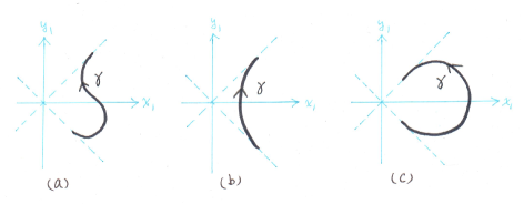
Figure 4: From (a) to (c): $\Delta\varphi=0,-\pi,\pi$; $d_{L_{\gamma}}=0,-2,2$.

Note that $c_{\tau}(L_{\gamma})$ and $L_{\gamma}$ have the same $\mu_{2}$-index (in fact they are Hamiltonian isotopic) and the precise value of $\mu_{2}$-index depends only on the variation $\Delta\varphi:=\varphi(b)-\varphi(a)$ but not on $\Delta t:=t(b)-t(a)$.

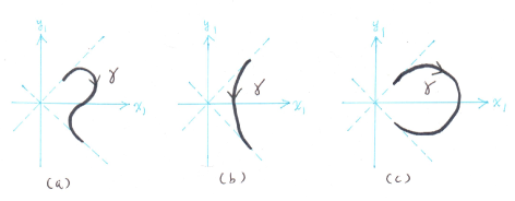
Figure 5: From (a) to (c): $\Delta\varphi=0,\pi,-\pi$; $d_{L_{\gamma}}=0,-2,2$.

Example for Case (ii):   Let $\gamma$ be as in the above example for Case (i) but with the opposite orientation, then $\varphi\in(\pi,2\pi)\mod 2\pi$ except at endpoints of $\gamma$. Here $V_{0}=V_{0,2}\cup V_{0,4}$ and $\check{\Gamma}_{0}\subset\partial V_{0}$ with the boundary orientation is

(24) $$\check{\Gamma}^{+}_{0}=-\gamma\cup\gamma_{\frac{\pi}{2}}\cup-\gamma_{\pi}\cup\gamma_{\frac{3\pi}{2}}.$$

The relative $E_{0}$-phase along each of the four components of $\check{\Gamma}^{+}_{0}$ is $-\Delta\varphi$, $\alpha_{0,2}=-2\Delta\varphi=\alpha_{0,4}$, and hence

(25) $$\mu_{2}(L_{\gamma}):=d_{L\gamma}=\frac{1}{2\pi}(\alpha_{0,2}+\alpha_{0,4})=\frac{1}{2\pi}(-4\Delta\varphi)=-\frac{2}{\pi}\Delta\varphi.$$

See Figure 5 for examples with $\Delta\varphi=\pm\pi$ or $0$.

Remark 5.1.2.

Note that in the above examples of $L_{\gamma}$, the orientation of $\check{\Gamma}^{+}_{0}$ (and hence of all $\check{\Gamma}^{+}_{\tau}$) does not depend on the orientation of $\gamma$.

5.1.2 Whitney sphere and tori

Lagrangian Whitney sphere.  Consider the polar curve $\gamma$ in $\mathbb{R}^{2}_{x_{1},y_{1}}$ defined by

$$y_{1}^{2}-\frac{x_{1}^{2}}{2}+\frac{x_{1}^{4}}{4}=0,\quad x_{1}\geq 0.$$

We orient $\gamma$ counterclockwise and parameterize it by its angular coordinate $t$ with $-\arctan\frac{1}{\sqrt{2}}\leq t\leq\arctan\frac{1}{\sqrt{2}}$. The immersed Lagrangian surface $L_{\gamma}:=Orb_{\mathcal{G}}(\gamma)$ is a Whitney sphere, an immersed sphere with one transversal positive self-intersection. We orient $L_{\gamma}$ so that $\dot{\gamma}$ and $X_{G}(\gamma)$ form a positive basis of $T_{\gamma}L_{\gamma}$ for $t\neq\pm\arctan\frac{1}{\sqrt{2}}$.

Note that $\gamma$ resembles the curve in Figure 4(c) except that here the endpoints of $\gamma$ meet at $(0,0)$, Still we have $\Delta\varphi=\pi$ along $\gamma$. There are no crossing $p$-curves in $L_{\gamma}$. Take $q$ to be any regular point of $L_{\gamma}$, then by (23)

$$\mu_{2}(L_{\gamma})=2=y(L_{\gamma},q).$$

Chekanov torus.  Consider the closed curve $\upsilon:=\sigma\cup\gamma$ in $\mathbb{R}^{2}_{x_{1},y_{1}}$:

$$\sigma(s) :=(x_{1}=\sqrt{2}r+r\cos s,y_{1}=r\sin s),\quad\frac{-3\pi}{4}\leq s\leq\frac{3\pi}{4},$$

$$\gamma(s) :=(x_{1}=\sqrt{2}r+r\cos s,y_{1}=r\sin s),\quad\frac{3\pi}{4}\leq s\leq\frac{5\pi}{4},$$

where $r>0$ is a constant. The orbit

$$L_{\upsilon}:=Orb_{\mathcal{G}}(\upsilon)$$

is a Chekanov torus.

Observe that $\sigma$ is as in Figure 4(c) with $(\Delta\varphi)_{\sigma}=\pi$, and $\gamma$ is as in Figure 5(b) with $(\Delta\varphi)_{\gamma}=\pi$. Both $L_{\sigma}$ and $L_{\gamma}$ are crossing domains of $L_{\upsilon}$. Let $q$ be a regular point in $L_{\sigma}$, then

$$\mu_{2}(L_{\upsilon}) =d_{L_{\sigma}}+d_{L_{\gamma}}=\frac{2}{\pi}((\Delta\varphi)_{\sigma}-(\Delta\varphi)_{\gamma}))=\frac{2}{\pi}(\pi-\pi)=0,$$

$$y(L_{\upsilon},q) =d_{L_{\sigma}}-d_{L_{\gamma}}=\frac{2}{\pi}((\Delta\varphi)_{\sigma}+(\Delta\varphi)_{\gamma}))=\frac{2}{\pi}(\pi+\pi)=4.$$

Monotone Clifford torus.  Let $\gamma^{\prime}:=M(\gamma)$, $\upsilon^{\prime}:=\sigma\cup\gamma^{\prime}$. Then $L_{\upsilon^{\prime}}=L_{\sigma}\cup L_{\gamma^{\prime}}\subset\mathbb{R}^{4}$ is a monotone Clifford torus. Observe that, up to a rotation by some $c_{\tau}\in\mathcal{C}$, $\gamma^{\prime}$ resembles the model curve in Figure 4(b) with $(\Delta\varphi)_{\gamma^{\prime}}=-\pi$. Note that both $L_{\sigma}$ and $L_{\gamma^{\prime}}$ are folding domains of $L_{\upsilon^{\prime}}$. Let $q$ be a regular point in $L_{\sigma}$, then

$$y(L_{\upsilon^{\prime}},q)=\mu_{2}(L_{\upsilon^{\prime}})=d_{L_{\sigma}}+d_{L_{\gamma^{\prime}}}=\frac{2}{\pi}((\Delta\varphi)_{\sigma}+(\Delta\varphi)_{\gamma^{\prime}}))=\frac{2}{\pi}(\pi-\pi)=0.$$

This in particular implies that the monotone Clifford torus $L_{\upsilon^{\prime}}$ is not Hamiltonian isotopic to the Chekanov torus $L_{\upsilon}$.

General Clifford torus.  There is another way to describe a monotone Clifford torus. A (not necessarily monotone) Clifford torus is defined as

$$T_{a,b}:=\{x_{1}^{2}+y_{1}^{2}=a,\ x_{2}^{2}+y_{2}^{2}=b\}\subset\mathbb{R}^{4},$$

where $a,b>0$ are constants. Then $T_{a,b}$ is monotone iff $a=b$. It is easy to see that with respect to the standard complex structure $J$ and the unitary framing $\partial_{x_{1}},\partial_{x_{2}}$, the image in $\mathbb{P}(K^{\prime})$ of $T_{a,b}$ under the map $g^{\prime}_{T_{a,b}}$ degenerates to a circle. Hence $\mu_{2}(T_{a,b})=0$ for any $a,b>0$. Also $y(T_{a,b},q)=0$ because $g^{\prime}_{T_{a,b}}$ is not surjective.

5.1.3 Fibers of an integrable system

It is possible to construct an integrable system whose Lagrangian fibers include a Whitney sphere, Chekanov tori, as well as Clifford tori. In this section we study the $\mu_{2}$ index and the $y$-index of Lagrangian fibers of such an integrable system in $\mathbb{R}^{4}$ defined by a pair of commutative Hamiltonian functions $G,H$ where

$$G(x_{1},y_{1},x_{2},y_{2}) := -x_{1}y_{2}+x_{2}y_{1},$$

$$H(x_{1},y_{1},x_{2},y_{2}) := y_{1}^{2}+y_{2}^{2}-\frac{1}{2}(x_{1}^{2}+x_{2}^{2})+\frac{1}{4}(x_{1}^{2}+x_{2}^{2})^{2}.$$

On can check that the Poisson bracket $\{H,G\}=0$, in other words, the Lie bracket of the corresponding Hamiltonian vector fields is $[X_{H},X_{G}]=0$. We remark here that a similar integrable system was considered by Bates in [3]. The example considered by Auroux in §5.1 of [2] is also topologically equivalent the one we consider here. Interested readers are advised to consult the references for more detail. Here we only state what are relevant to our purpose.

The pair $(G,H)$ defines a map by assigning to $p\in\mathbb{R}^{4}$ its $(G,H)$-values.

$$\mathcal{Z}:\mathbb{R}^{4}\to\mathbb{R}^{2},\quad\Xi(p):=(G(p),H(p)).$$

Let $\mathcal{R}$ denote the range of $\mathcal{Z}$. It is an unbounded closed domain of $\mathbb{R}^{2}$. The boundary $\partial\mathcal{R}$ is a smooth curve containing the point $(0,-\frac{1}{4})$ where $-\frac{1}{4}$ is the minimum value of $H$. The two vector fields $X_{G}$ and $X_{H}$ are linearly independent except at $\mathcal{Z}^{-1}(\partial\mathcal{R})$ where $X_{H}$ and $X_{G}$ are nonvanishing but linearly dependent, and at the origin $0\in\mathbb{R}^{4}$ at which $X_{G}=0=X_{H}$. Both $X_{G}$ and $X_{H}$ are tangent to fibers of $\mathcal{Z}$. Let $L_{a,b}:=\mathcal{Z}^{-1}(a,b)$ denote the fiber of $\mathcal{Z}$ over $(a,b)\in\mathcal{R}$. For $(a,b)\in\partial\mathcal{R}$, $L_{a,b}$ is degenerate and is diffeomorphic to $S^{1}$. In addition, we have the following observation concerning the Lagrangian fibers over interior points of $\mathcal{R}$:

Fact 5.1.3.

Let $int(\mathcal{R})$ denote the interior of $\mathcal{R}$. Then there are four types of Lagrangian fibers over $(a,b)\in int(\mathcal{R})$:

1. $L_{a,b}$ is a Chekanov torus if $a=0$ and $-\frac{1}{4}<b<0$.

2. $L_{a,b}$ is a monotone Clifford torus if $a=0$ and $b>0$.

3. $L_{a,b}$ is a Lagrangian Whitney sphere if $(a,b)=(0,0)$.

4. $L_{a,b}$ is a non-monotone embedded Lagrangian torus for all $(a,b)\in int(\mathcal{R})$ with $a\neq 0$.

Recall that $X_{G}$ generates the $\mathcal{G}$-action on $\mathbb{R}^{4}$, with $g_{\theta}$ as the time $\theta$ map of the flow of $X_{G}$. Thus all $L_{a,b}$ are $\mathcal{G}$-invariant.

We have the following result concerning the $y$-index of $L_{a,b}$ for $(a,b)\in\mathcal{R}^{\circ}$.

Proposition 5.1.4.

Let $(a,b)\in int(\mathcal{R})$. Then the pair

$$(\mu_{2}(L_{a,b}),\ \bar{y}(L_{a,b}))=\begin{cases}(0,4)&\text{ if $a=0$ and $-\frac{1}{4}<b<0$},\\ (2,2)&\text{ if $a=0=b$},\\ (0,0)&\text{ if $a=0$ and $B>0$},\\ (0,0)&\text{ if $a\neq 0$.}\end{cases}$$

Proof.

Consider the case of $a=0$ at first. Let $h:\mathbb{R}^{2}_{x_{1},y_{1}}\to\mathbb{R}$,

$$h(x_{1},y_{1}):=y_{1}^{2}-\frac{1}{2}x_{1}^{2}+\frac{1}{4}x_{1}^{4},$$

denote the restriction of $H$ to $\mathbb{R}^{2}_{x_{1},y_{1}}$. Then $L_{0,b}=L_{\gamma_{b}}:=Orb_{\mathcal{G}}(\gamma_{b})$ where

$$\gamma_{b}=h^{-1}(b)\cap\{x_{1}\geq 0\}.$$

By analyzing level curves of $h$ it is easy to see that $L_{0,b}$ is Hamiltonian isotopic to a Chekanov torus if $b<0$, a Whitney sphere if $b=0$ and a monotone Clifford torus if $b>0$. So it remains to prove the case of $a\neq 0$.

Let $(a,b)\neq(0,0)$ be an interior point of of $\mathcal{R}$. Then $TL_{a,b}=\text{Span}\{X_{G},X_{H}\}$ where, with respect to the basis $\{\partial_{x_{1}},\partial_{x_{2}},\partial_{y_{1}},\partial_{y_{2}}\}$,

$$X_{G} =(-x_{2},x_{1},-y_{2},y_{1})^{T},$$

$$X_{H} =(-2y_{1},-2y_{2},x_{1}(x_{1}^{2}+x_{2}^{2}-1),x_{2}(x_{1}^{2}+x_{2}^{2}-1))^{T}.$$

Recall the $\mathcal{G}$-invariant $S^{1}$-family of complex planes $E_{\theta}$. Since $L_{a,b}$ is also $\mathcal{G}$-invariant, the locus $\Gamma_{\theta}\subset L_{a,b}$ of $E_{\theta}$ is $g_{\theta}(\Gamma_{0})$, it is enough to analyze the intersection subspaces along $\Gamma_{0}$. Since $E_{0}=\partial_{x_{1}}\wedge\partial_{y_{1}}$, $p:=(x_{1},y_{1},x_{2},y_{2})\in\Gamma_{0}$ iff it satisfies the defining equations of $L_{a,b}$: $G=a$, $H=b$, and the determinant of the $4\times 4$ matrix $\begin{pmatrix}X_{H}&X_{G}&\partial_{x_{1}}&\partial_{y_{1}}\end{pmatrix}$ vanishes at $p$, i.e.,

(26) $$x_{1}x_{2}(x_{1}^{2}+x_{2}^{2}-1)+2y_{1}y_{2}=0.$$

Consider two vector fields $Z_{1},Z_{2}$ on $\mathbb{R}^{4}$ defined by

$$Z_{1}=(0,x_{1},0,y_{1})^{T},\quad(x_{2},0,y_{2},0)^{T}.$$

Observe that both $Z_{1}$ and $Z_{2}$ are $\mathcal{G}$-invariant, $Z_{1}-Z_{2}=X_{G}$, their inner product is $Z_{1}\cdot Z_{2}=0$, and $Z_{1},Z_{2}$ are linearly independent precisely at points where $x_{1}^{2}+y_{1}^{2}>0$ and $x_{2}^{2}+y_{2}^{2}>0$. In particular this include all points with $a\neq 0$. We have

$$dG(Z_{1})=dG(Z_{2}) =0$$

$$dH(Z_{1})=dH(Z_{2}) =x_{1}x_{2}(x_{1}^{2}+x_{2}^{2}-1)+2y_{1}y_{2}.$$

So for $p\in L_{a,b}$ and $i=1,2$,

$$Z_{i}(p)\in T_{p}L_{a,b}\quad\Leftrightarrow\quad p\in\Gamma_{0}=\Gamma_{\frac{\pi}{2}},$$

and in this case,

$$Z_{2}(p)\in T_{p}L_{a,b}\cap E_{0},\quad Z_{1}(p)\in T_{p}L_{a,b}\cap E_{\frac{\pi}{2}}.$$

Since $L_{a,b}$ are smoothly isotopic as Lagrangian surfaces for all $(a,b)\neq(0,0)$, and $\mu_{2}$-index is invariant under regular homotopy of Lagrangian surfaces, we have $\mu_{2}(L_{a,b})=0$ for all $(a,b)\neq(0,0)$. To determine $\bar{y}(L_{a,b})$ with $a\neq 0$, observe that $a=x_{2}y_{1}-x_{1}y_{2}\neq 0$, hence along $\Gamma_{0}$ the angle of $Z_{2}$ in $E_{0}$ (with respect to $\partial_{x_{1}}$) minus the angle of $Z_{1}$ in $E_{\frac{\pi}{2}}$ (with respect to $\partial_{x_{2}}$) is always

1. greater than $0$ but smaller than $\pi$-radians if $a>0$,

2. greater than $-\pi$ but smaller than $0$-radians if $a<0$.

So the entire $T_{a,b}$ is a crossing domain and moreover the map $g^{\prime}_{T_{a,b}}:T_{a,b}\to\mathbb{P}(K^{\prime})$ is not surjective. Therefore

$$\bar{y}(T_{a,b})=y(T_{a,b})=\mu_{2}(T_{a,b})=0.$$

This completes the proof of Proposition 5.1.4. ∎

5.2 Sphere in $T^{*}S^{2}$

Let $S$ denote the zero section of the cotangent bundle $T^{*}S^{2}$ of a sphere, $T^{*}S^{2}$ is endowed with the standard symplectic structure $\omega$. Note that $T^{*}S^{2}$ is symplectically parallelizable, and $H_{1}(T^{*}S^{2},\mathbb{Z})=0=H_{3}(T^{*}S^{2},\mathbb{Z})$, so its $\mathcal{F}^{\omega}$ is connected, and $\mu_{2}(S,\EuFrak{f})$ is independent of $\EuFrak{f}\in\mathcal{F}^{\omega}$.

We identify $S=D\cup\bar{D}$ as the union of two closed Lagrangian disks $D$ and $\bar{D}$. Parametrize $D$ and $\bar{D}$ as

$$D =\{(x_{1},x_{2})\in\mathbb{R}^{2}\mid x_{1}^{2}+x_{2}^{2}\leq 1\},$$

$$\bar{D} =\{(\bar{x}_{1},\bar{x}_{2})\in\mathbb{R}^{2}\mid\bar{x}_{1}^{2}+\bar{x}_{2}^{2}\leq 1\}$$

We also write $x_{1}=r\cos\theta$ and $x_{2}=r\sin\theta$ where $(r,\theta)$ are polar coordinates of $\mathbb{R}^{2}_{x_{1}x_{2}}$. Similarly $\bar{x}_{1}=\bar{r}\cos\bar{\theta}$ and $\bar{x}_{2}=\bar{r}\sin\bar{\theta}$ where $(\bar{r},\bar{\theta})$ are polar coordinates of $\mathbb{R}^{2}_{\bar{x}_{1}\bar{x}_{2}}$.

Consider the diffeomorphism $\psi:\bar{D}\setminus\{0\}\to D\setminus\{0\}$

(27) $$\psi(\bar{x}_{1},\bar{x}_{2})=\Big{(}x_{1}=\frac{-\bar{x}_{1}}{\bar{x}_{1}^{2}+\bar{x}_{2}^{2}},x_{2}=\frac{\bar{x}_{2}}{\bar{x}_{1}^{2}+\bar{x}_{2}^{2}}\Big{)},\quad 0<\bar{x}_{1}^{2}+\bar{x}_{2}^{2}\leq 1.$$

In polar coordinates $\psi(\bar{r},\bar{\theta})=(r=\frac{1}{\bar{r}},\theta=\pi-\bar{\theta})$. $\psi$ induces a symplectomorphism

$$\Psi :T^{*}(\bar{D}\setminus\{0\})\to T^{*}(D\setminus\{0\})$$

$$\Psi(\bar{x}_{1},\bar{x}_{2},(\bar{y}_{1},\bar{y}_{2})^{T}) =(\psi(\bar{x}_{1},\bar{x}_{2}),(\psi_{*}^{-1})^{*}_{(\bar{x}_{1},\bar{x}_{2})}(\bar{y}_{1},\bar{y}_{2})^{T}).$$

The differential $\Psi_{*}$, in matrix form with respect to the bases $\{\partial_{\bar{x}_{1}},\partial_{\bar{x}_{2}},\partial_{\bar{y}_{1}},\partial_{\bar{y}_{2}}\}$ and $\{\partial_{x_{1}},\partial_{x_{2}},\partial_{y_{1}},\partial_{y_{2}}\}$ is

$$\Psi_{*}|_{(\bar{x},\bar{y})} =\begin{pmatrix}B&0\\ 0&(B^{-1})^{T}\end{pmatrix}\in Sp(4,\mathbb{R}),\quad\text{where}$$

$$B =\begin{pmatrix}x_{1}^{2}-x_{2}^{2}&-2x_{1}x_{2}\\ 2x_{1}x_{2}&x_{1}^{2}-x_{2}^{2}\end{pmatrix}=r^{2}\begin{pmatrix}\cos 2\theta&-\sin 2\theta\\ \sin 2\theta&\cos 2\theta\end{pmatrix}.$$

Note that $B$ and hence $\Psi_{*}$ depend only on $x=(x_{1},x_{2})$, not on $y=(y_{1},y_{2})$. The symplectic manifold $T^{*}S^{2}$ can be identified with the union $T^{*}D\cup_{\Psi}T^{*}\bar{D}$.

We identify each of $T^{*}D$ and $T^{*}\bar{D}$ as open domains in $T^{*}\mathbb{R}^{2}\cong\mathbb{C}^{2}$. Let $X_{i}:=\partial_{x_{i}}$ and $\bar{X}_{i}:=\partial_{\bar{x}_{i}}$ for $i=1,2$. On $T^{*}D$ the ordered pair $(X_{1},X_{2})$ is a unitary framing with respect to the standard complex structure $J$, and similarly $(\bar{X}_{1},\bar{X}_{2})$ is a unitary framing on $T^{*}\bar{D}$ with respect to the standard complex structure which is now denoted as $\bar{J}$ to suggest its affinity with $T^{*}\bar{D}$. Note that $\Psi^{*}\bar{J}=J$ on $T^{*}_{\partial D}D=\{(x,y)\in\mathbb{R}^{2}\times\mathbb{R}^{2}\mid|x|=1\}$, $J$ and $\bar{J}$ match along $T^{*}_{\partial D}D$ to form a $\omega$-compatible almost complex structure denoted as $J$ on $T^{*}S^{2}$. However the two unitary bases do not:

$$\begin{pmatrix}\bar{X}_{1}&\bar{X}_{2}\end{pmatrix}=\begin{pmatrix}\cos 2\theta&-\sin 2\theta\\ \sin 2\theta&\cos 2\theta\end{pmatrix}\begin{pmatrix}X_{1}&X_{2}\end{pmatrix}\quad\text{ on $T^{*}_{\partial D}D$}.$$

Unitary framing $(u,v)$.  We will modify $X_{1},X_{2}$ on $T^{*}D$ to get a unitary framing $u,v$ on $T^{*}S^{2}$ so that $u=\bar{X}_{1}$ and $v=\bar{X}_{2}$ on $T^{*}\bar{D}$. Observe that $B|_{r=1}$ is twice of the contractible loop

$$G_{0}(\vartheta):=\begin{pmatrix}\cos\vartheta&-\sin\vartheta\\ \sin\vartheta&\cos\vartheta\end{pmatrix}\in SU(2)\cong S^{3},\quad\vartheta\in\mathbb{R}/2\pi\mathbb{Z}.$$

Moreover, any two homotopies between $G_{0}$ and the constant loop $Id$ in $SU(2)$ are homotopic. Construct a homotopy between $G_{0}$ and $Id$ as follows: Let

$$H(t):=\begin{pmatrix}\cos t&i\sin t\\ i\sin t&\cos t\end{pmatrix}\in SU(2)$$

and define

(28) $$G_{t}(\vartheta):=H(t)G_{0}(\vartheta)H(t)^{-1}.$$

Note that $G_{t+\pi}(\vartheta)=G_{t}(\vartheta)$, $G_{t+\frac{\pi}{2}}(\vartheta)=G_{t}(-\vartheta)=G_{t}(\vartheta)^{-1}$. In matrix form with respect to the basis $\{\partial_{x_{1}},\partial_{x_{2}},\partial_{y_{1}},\partial_{y_{2}}\}$

$$G_{t}(\vartheta)=\begin{pmatrix}\cos\vartheta&-\sin\vartheta\cos 2t&-\sin\vartheta\sin 2t&0\\ \sin\vartheta\cos 2t&\cos\vartheta&0&\sin\vartheta\sin 2t\\ \sin\vartheta\sin 2t&0&\cos\vartheta&-\sin\vartheta\cos 2t\\ 0&-\sin\vartheta\sin 2t&\sin\vartheta\cos 2t&\cos\vartheta\end{pmatrix}.$$

The set

$$\mathcal{D}:=\{G_{t}(\vartheta)\mid\vartheta\in[0,\pi],\ t\in[0,\frac{\pi}{2}]\}\subset SU(2)$$

is a hemisphere with boundary the group $G_{0}$.

For the moment let us consider the diffeomorphism

$$f :\mathcal{D}\to D$$

$$f(G_{t}(\vartheta)) :=(x_{1}=\cos\vartheta,x_{2}=\sin\vartheta\cos 2t)$$

Consider a new unitary framing $u^{\prime},v^{\prime}$ over $D$ so that if $f^{-1}(x)=G_{t}(\vartheta)$ for $x\in D$, then

(29) $$u^{\prime}_{x}:=G_{t}(\vartheta)(\partial_{x_{1}}),\quad v^{\prime}_{x}:=G_{t}(\vartheta)(\partial_{x_{2}}).$$

Note that $u^{\prime}\wedge v^{\prime}\in\mathbb{P}(K^{\prime})$. Observe that $\partial D=f(\{t=0,\frac{\pi}{2}\})$. Recall $x=(x_{1},x_{2})=(r\cos\theta,r\sin\theta)$, then along $f(\{t=0\})=\{r=1,\theta\in[0,\pi]\}$, $\vartheta=\theta$, and

$$u^{\prime}_{x} =\cos\theta\partial_{x_{1}}+\sin\theta\partial_{x_{2}}$$

$$v^{\prime}_{x} =-\sin\theta\partial_{x_{1}}+\cos\theta\partial_{x_{2}}.$$

Similarly, along $f(\{t=\frac{\pi}{2}\})=\{r=1,\ \theta\in[-\pi,0]\}$, $\vartheta=-\theta$ and

$$u^{\prime}_{x} =\cos\theta\partial_{x_{1}}+\sin\theta\partial_{x_{2}}$$

$$v^{\prime}_{x} =-\sin\theta\partial_{x_{1}}+\cos\theta\partial_{x_{2}}.$$

Also, along the diameter $x_{2}=0$ and at $x_{1}=\cos\vartheta$,

(30) $$u^{\prime}_{x}=\cos\vartheta\partial_{x_{1}}+\sin\vartheta\partial_{y_{1}},\quad v^{\prime}_{x}=\cos\vartheta\partial_{x_{2}}-\sin\vartheta\partial_{y_{2}}.$$

Now consider the composite map

(31) $$F:=f^{-1}\circ\phi:D\to\mathcal{D}$$

where

(32) $$\phi:D\to D,\quad\phi(x_{1},x_{2}):=(x_{1}^{2}-x_{2}^{2},2x_{1}x_{2})$$

is the standard branched $2:1$ covering map of degree $2$ with $(0,0)$ as the only branching point. $F(x_{1},x_{2})=G_{t}(\vartheta)$ if

(33) $$x_{1}^{2}-x_{2}^{2}=\cos\vartheta,\quad 2x_{1}x_{2}=\sin\vartheta\cos 2t.$$

For $x\in D$ define

(34) $$u_{x}:=G_{t}(\vartheta)(\partial_{x_{1}}),\quad v_{x}:=G_{t}(\vartheta)(\partial_{x_{2}}),\quad\text{ if $F(x)=G_{t}(\vartheta)$}.$$

A direction computation shows that along $\partial D$,

$$u_{x} =\cos 2\theta\partial_{x_{1}}+\sin 2\theta\partial_{x_{2}}=\partial_{\bar{x}_{1}},$$

$$v_{x} =-\sin 2\theta\partial_{x_{1}}+\cos 2\theta\partial_{x_{2}}=\partial_{\bar{x}_{2}}.$$

Extend $(u,v)$ over $\bar{D}$ by setting

$$u=\partial_{\bar{x}_{1}},\quad v=\partial_{\bar{x}_{2}}\quad\text{ on }\bar{D},$$

then further extend $(u,v)$ over $T^{*}S$ by the pullback map of the canonical projection $\pi:T^{*}S\to S=\bar{D}\cup_{\psi}D$. Now the extended $(u,v)$ is a unitary framing on $T^{*}S$.

$E^{\prime}_{s}$ associated to $(u,v)$.  Let $\mathcal{E}^{\prime}:=\{E^{\prime}_{s}\mid s\in\mathbb{R}/\pi\mathbb{Z}\}$ denote the $S^{1}$-family of complex line bundles associated to the unitary framing $(u,v)$. Recall the $S^{1}$-family of complex line bundles $\mathcal{E}:=\{E_{s}\mid s\in\mathbb{R}/\pi\mathbb{Z}\}$, associated to the unitary framing $\partial_{x_{1}},\partial_{x_{2}}$. Then at $(x,y)\in T^{*}D$,

$$E^{\prime}_{s}|_{(x,y)}=G_{t}(\vartheta)(E_{s}|_{(x,y)})\quad\text{ if $F(x)=(G_{t}(\vartheta))$}.$$

Since $TD$ is spanned by $\partial_{x_{1}},\partial_{x_{2}}$, for $x\in D$, there exists $s^{\prime}\in\mathbb{R}/\pi\mathbb{Z}$, $s^{\prime}$ depends on $x$, such that

(35) $$\{E^{\prime}_{s},E^{\prime}_{s^{\perp}}\}=\{E_{s^{\prime}},E_{{s^{\prime}}^{\perp}}\}\quad\text{ at $x\in D$}.$$

To solve for $s,s^{\prime}$ with

(36) $$E_{s^{\prime}}=G_{t}(\vartheta)(E_{s}),$$

observe that the two fixed points of the action of $H$ on $\mathbb{P}(J)$ are

$$E_{\frac{\pi}{4}}=(\partial_{x_{1}}+\partial_{x_{2}})\wedge(\partial_{y_{1}}+\partial_{y_{2}}),\quad E_{\frac{3\pi}{4}}=E_{{\frac{\pi}{4}}^{\perp}}=(-\partial_{x_{1}}+\partial_{x_{2}})\wedge(-\partial_{y_{1}}+\partial_{y_{2})}.$$

$H(t)$ rotates the tangent plane $T_{E_{\frac{\pi}{4}}}\mathbb{P}(J)$ clockwise by an angle of $2t$-radians. We take the fixed points of the $G_{0}$-action on $\mathbb{P}(J)$ as the poles of $\mathbb{P}(J)$. Then $\mathcal{E}\subset\mathbb{P}(J)$ is the equator. Assume that $t,s\in(0,\frac{\pi}{4})$ for the moment. Consider the right spherical triangle in $\mathbb{P}(J)$ cut out by $\mathcal{E}$, $H(-t)(\mathcal{E})$ and the longitude $\ell_{t,s}$ passing through the point $H(-t)(E_{s})$. The point $H(-t)(E_{s})$ is on a latitude $m_{t,s}$ (an $G_{0}$-orbit) of $\mathbb{P}(J)$. Let $E_{\tau}$ denote the intersection point of $\ell_{t,s}$ with $\mathcal{E}$. $E_{\tau}$ is the right angle vertex of the triangle, $0<s<\tau$. Scale $\mathbb{P}(J)$ to make it a sphere of radius 1. Then the angle at the vertex $E_{\frac{\pi}{4}}$ is $2t$, the length of the side opposite to the vertex $E_{\tau}$ is $\frac{\pi}{2}-2s$, and the length of the side opposite to the vertex $H(-t)(E_{s})$ is $\frac{\pi}{2}-2\tau$. We have

$$\cos 2t=\tan(\frac{\pi}{2}-2\tau)\cot(\frac{\pi}{2}-2s)=\cot 2\tau\tan 2s$$

according to spherical trigonometry.

Since $H(-t)(E_{s^{\prime}})=G_{0}(\vartheta)H(-t)(E_{s})$, by considering the action of $G_{0}$ on its orbits in $\mathbb{P}(J)$ we must have

$$\vartheta=-2\tau\mod\pi,$$

and

(37) $$s^{\prime}=\pi-s\mod\pi.$$

Then $t$, $s$ and $\vartheta$ satisfy

(38) $$\cos 2t=-\tan 2s\cot\vartheta.$$

In fact Equations (37) and (38) hold for any $2t,\theta\in[0,\pi]$ and $s,s^{\prime}\in\mathbb{R}/\pi\mathbb{Z}$ satisfying Equation (36). Together with (33) we obtain that on $T^{*}D$

(39) $$E^{\prime}_{s}=E_{\pi-s}\ \text{ if }\tan 2s=\frac{-2x_{1}x_{2}}{x_{1}^{2}-x_{2}^{2}}.$$

In particular, on $\{x_{1}x_{2}=0\}\subset T^{*}D$

(40) $$E^{\prime}_{0}=E_{0}=\partial_{x_{1}}\wedge\partial_{y_{1}},\quad E^{\prime}_{\frac{\pi}{2}}=E_{\frac{\pi}{2}}=\partial_{x_{2}}\wedge\partial_{y_{2}}.$$

$\mu_{2}$- and $y$-indexes.  Now consider the $4\times 4$ matrix formed by column vectors $u^{\prime}$, $v^{\prime}$, $\cos s^{\prime}\partial_{x_{1}}+\sin s^{\prime}\partial_{x_{2}}$, and $\cos s^{\prime}\partial_{y_{1}}+\sin s^{\prime}\partial_{y_{2}}$ with $s^{\prime}=\pi-s$, of which the determinant is

$$\begin{split}\EuFrak{D}^{\prime}&:=\begin{vmatrix}\cos\vartheta&-\sin\vartheta\cos 2t&\cos s^{\prime}&0\\ \sin\vartheta\cos 2t&\cos\vartheta&\sin s^{\prime}&0\\ \sin\vartheta\sin 2t&0&0&\cos s^{\prime}\\ 0&-\sin\vartheta\sin 2t&0&\sin s^{\prime}\end{vmatrix}\\ &=\sin\vartheta\sin 2t\cdot(\cos 2t\cos 2s^{\prime}\sin\vartheta-\sin 2s^{\prime}\cos\vartheta)\\ &=\sin\vartheta\sin 2t\cdot(\cos 2t\cos 2s\sin\vartheta+\sin 2s\cos\vartheta).\end{split}$$

$\EuFrak{D}^{\prime}=0$ iff one of the followings folds:

1. $\vartheta=0$ or $\pi$,

2. $t=0$ or $\frac{\pi}{2}$,

3. $\vartheta=\frac{\pi}{2}$ and $t=\frac{\pi}{4}$,

4. $\cos 2t\cos 2s\sin\vartheta=-\sin 2s\cos\vartheta$.

In (i)-(iii) $\EuFrak{D}^{\prime}=0$ for all values of $s$. Moreover, (i) holds at four points of $\partial D$, (ii) holds precisely on $\partial D$, and (iii) corresponds to the origin of $D$. Consider the PLG-map

$$g^{\prime}_{D}:D\to\mathbb{P}(K^{\prime})$$

with respect to the framing $(u,v)$ so that $\xi^{\prime}_{0}:=u\wedge v$ is viewed as the south pole of $\mathbb{P}(K^{\prime})$ and $\xi^{\prime}_{\infty}:=Ju\wedge-Jv$ the north pole. Then $g^{\prime}_{D}$ is surjective with

$$(g^{\prime}_{D})^{-1}(\xi^{\prime}_{0})=\partial D,\quad(g^{\prime}_{D})^{-1}(\xi^{\prime}_{\infty})=(0,0)\in D.$$

It is easy to see that $\deg g^{\prime}=\pm 2$. To determine the $\pm$ sign of $\deg g^{\prime}_{D}$ we consider Case (iv) which implies that (recall (33), (40))

$$\tan 2s=\frac{-\sin\vartheta\cos 2t}{\cos\vartheta}=\frac{-2x_{1}x_{2}}{x^{2}_{1}-x_{2}^{2}}.$$

Hence the intersection of $\Gamma_{s}:=(g^{\prime}_{D})^{-1}(\lambda_{s})$ with the interior $int(D)$ of $D$ is the pair of orthogonal line segments defined by $-2x_{1}x_{2}=(x_{1}^{2}-x_{2}^{2})\tan 2s$, $x_{1}^{2}+x_{2}^{2}<1$.

Take $s=0$, then $V_{0}:=(g^{\prime}_{D})^{-1}(D_{0})=\{x_{1}x_{2}>0\}\cap D$. Write $V_{0}=V_{01}\cup V_{02}$, where $V_{01}=V_{0}\cap\{x_{2}>0\}$, $V_{02}=V_{0}\cap\{x_{2}<0\}$.

The boundary $\partial V_{01}\cap int(D)=\gamma\cup\sigma$, where

$$\gamma(t) =(x_{1}=0,x_{2}=\cos 2t),\quad 0<t\leq\frac{\pi}{4};$$

$$\sigma(t) =(x_{1}=-\cos 2t,x_{2}=0),\quad\frac{\pi}{4}\leq t<\frac{\pi}{2}.$$

Observe that the map $\phi$ from (32) maps $\gamma\cup\sigma$ onto the diameter $\{x_{2}=0\}\cap int(D)$ injectively. By (30) along $\gamma\cup\sigma$

$$\begin{pmatrix}u&v\end{pmatrix}=\begin{pmatrix}-\cos 2t&0\\ 0&-\cos 2t\\ \sin 2t&0\\ 0&-\sin 2t\end{pmatrix},\ 0<t<\frac{\pi}{2},$$

$\partial_{x_{1}}$ generates the intersection subspace of $E^{\prime}_{0}:=u\wedge Ju=E_{0}=\partial_{x_{1}}\wedge\partial_{y_{1}}$, $\partial_{x_{1}}=-(\cos 2t)u-(\sin 2t)Ju$, whilst $\partial_{x_{2}}$ generates the intersection subspace of $E^{\prime}_{\frac{\pi}{2}}:=v\wedge Jv=E_{\frac{\pi}{2}}=\partial_{x_{2}}\wedge\partial_{y_{2}}$, $\partial_{x_{2}}=(\cos 2t)v-(\sin 2t)Jv$. So as $t$ increases from $0$ to $\frac{\pi}{2}$, $\partial_{x_{1}}$ rotates in $E^{\prime}_{0}$ by an angle of $\pi$ radians, and $\partial_{x_{2}}=$ rotates in $E^{\prime}_{\frac{\pi}{2}}$ by an angle of $-\pi$ radians. We have

$$\alpha_{01}=(\Delta\varphi)_{\gamma\cup\sigma}=\pi-(-\pi)=2\pi,$$

the restricted map

$$g^{\prime}_{S}\mid_{\partial V_{01}}:\partial V_{01}\to\lambda^{+}_{0}$$

is of degree 1. Similarly, the the restricted map

$$g^{\prime}_{S}\mid_{\partial V_{02}}:\partial V_{02}\to\lambda^{+}_{0}$$

is also of degree 1. These put together imply that the $\mu_{2}$-index of the zero-section $S$ of $T^{*}S$ (with respect to the framing $\EuFrak{f}:=(J,u,v)$) is

$$\mu_{2}(S)=2.$$

There are no crossing $p$-curves on $S$. Take a regular point $q\in S$ and we have

$$y(S,q)=\mu_{2}(S)=2.$$

Plumbing of $T^{*}S^{2}$’s.  Our construction of a unitary framing on $T^{*}S^{2}$ can be generalized to symplectic manifolds formed by plumbing a finite number of $T^{*}S^{2}$’s. For example, for any integer $n\geq 1$ consider the Stein surface $W_{n}\subset\mathbb{C}^{3}$ defined by the equation

(41) $$z_{1}^{2}+z_{2}^{2}=z_{3}^{n+1}+\frac{1}{2}.$$

$W_{n}$ is the plumbing of $n$ copies of $T^{*}S^{2}$ so that the Lagrangian zero-section spheres $S_{1}$,…,$S_{n}$ form an $A_{n}$-configuration: $S_{j}\pitchfork S_{j+1}$ and in one point, $S_{i}\cap S_{j}=\emptyset$ if $|i-j|\neq 1$. Note that each of $W_{n}$ is a parallelizable symplectic 4-manifold, and their space of compatible unitary framings are all connected. It is not hard to see that

$$\mu_{2}(S_{j})=2=y(S_{j}),\quad j=1,...,n.$$

Moreover, we can orient the pair $S_{j},S_{j+1}$ so that their intersection is positive. Then by the lagrangian surgery as defined in [17] we can desingularize the double point of $S_{j}\cup S_{j+1}$ to get a smooth Lagrangian sphere. There are two different desingularizations. Call the resulting Lagrangian spheres as $S^{\prime}_{j}$ and $S^{\prime\prime}_{j}$. $S^{\prime}_{j}$ and $S^{\prime\prime}_{j}$ are related by a $la$-disk surgery, so $\mu_{2}(S^{\prime}_{j})=\mu_{2}(S^{\prime\prime}_{j})$. To determine $\mu_{2}(S^{\prime}_{j})$, recall that as we desingularize a Lagrangian Whitney sphere in $\mathbb{R}^{4}$ the $\mu_{2}$-index is decreased by 2. Then a simple calculation yields

$$\mu_{2}(S^{\prime}_{j})=\mu_{2}(S^{\prime\prime}_{j})=\mu_{2}(S_{j})+\mu_{2}(S_{j+1})-2=2.$$

5.3 Surfaces in the plumbing of cotangent bundles

We consider the following example to illuminate the effect of generalized Dehn twists on the relative $y$-index.

Let $L$ be an orientable compact surface without boundary, and $S$ a $2$-dimensional sphere. Let $W$ be the symplectic manifold obtained by plumbing the two symplectic manifolds $T^{*}L$ and $T^{*}S$ at a single point $p_{0}\in W$. $W$ is symplectically parallelizable, with Lagrangian surfaces $L$ and $S$ intersect transversally and at $p_{0}$.

Framing $\EuFrak{f}=(J,u,v)$.  We choose a framing $\EuFrak{f}=(J,u,v)$ for $TW$ so that on $T^{*}S$ it is a slight modification of our earlier construction. Recall from Section 5.2 $G_{t}(\theta)\subset SU(2)$, $t\in[0,\frac{\pi}{2}]$, $\theta\in[0,\pi]$, and $S=D\cup_{\psi}\bar{D}$, $\bar{D}=\{(\bar{x}_{1},\bar{x}_{2})\mid\bar{x}_{1}^{2}+\bar{x}_{2}^{2}\leq 1\}$ $D=\{(x_{1},x_{2})\mid x_{1}^{2}+x_{2}^{2}\leq 1\}$. We may assume that $p_{0}$ is in the interior of $\bar{D}$. We also write $x_{1}=r\cos\theta$, $x_{2}=r\sin\theta$, $(r,\theta)$ are polar coordinates of $D$. Let $p_{0}=(0,0)\in\bar{D}$ denote the south pole of $S$, and $p_{\infty}:=(0,0)\in D$ the north pole. Let $C\subset S$ denote the great circle so that $C\cap\bar{D}=\{\bar{x}_{2}=0\}$, $C\cap D=\{x_{2}=0\}$.

Consider the smooth surjective map $\rho_{D}:D\to D$,

$$\rho_{D}(r,\theta)=(\rho(r),\theta),$$

where $\rho:[0,1]\to[0,1]$ is a smooth function such that

• $\rho(r)=0$ on $[0,\epsilon)$ and $\rho(r)=1$ on $(1-\epsilon,1]$ for some $\epsilon>0$,

• $\frac{d\rho}{dr}\geq 0$.

For $x\in D$ define

(42) $$u_{x}=G_{t}(\theta)(\partial_{x_{1}}),\quad v_{x}:=G_{t}(\theta)(\partial_{x_{2}}),\quad\text{if $F(\rho_{D}(x))=G_{t}(\theta)$}.$$

Note that

$$(u,v)=\begin{cases}(\partial_{y_{1}},-\partial_{y_{2}})&\text{ if $r<\epsilon$ },\\ (\partial_{\bar{x}_{1}},\partial_{\bar{x}_{2}})&\text{ if $r=1$}.\end{cases}$$

Extend $u,v$ over $\bar{D}$ by setting $u=\partial_{\bar{x}_{1}}$ and $v=\partial_{\bar{x}_{2}}$ as before. Then further extend $u,v$ over $T^{*}S$ independent of fiber coordinates or, more precisely, by pulling back $u,v$ over $T^{*}S$ via the canonical projection $\pi:T^{*}S\to S$. Finally extend $J$ and $u,v$ over $T^{*}L$. We denote the resulting framing by $\EuFrak{f}:=(J,u,v)$. Let $E^{\prime}_{s}$ denote the $S^{1}$-family of $J$-complex line bundles associated to $u,v$. Write $u_{s}:=u\cos s+v\sin s$, $v_{s}=Ju_{s}$.

Let $\Gamma_{s}(S)$ denote the $E^{\prime}_{s}$-locus of $S$. $\Gamma_{s}(S)$ is the union of $\bar{D}\cup\{(r,\theta)\in D\mid\rho(r)=0\text{ or }1\}$ and a pair of great circles on $S$ intersects orthogonally at the poles $p_{0},p_{\infty}$. With (39) we can write this pair of great circles as $C_{s}\cup C^{\perp}_{s}$, where $C_{s}$ is the great circle tangent to $E^{\prime}_{s}$ (and orthogonal to $E^{\prime}_{s^{\perp}}$), and $C^{\perp}_{s}$ the one tangent to $E^{\prime}_{s^{\perp}}$ (and orthogonal to $E^{\prime}_{s}$). Then $C^{\perp}_{s}=C_{s^{\perp}}$. In particular, $C_{0}=C=\{x_{2}=0\}\cup\{\bar{x}_{2}=0\}$, $C^{\perp}_{0}=\{x_{1}=0\}\cup\{\bar{x}_{1}=0\}$.

$S^{1}$-action on $T^{*}S$.  Consider an $S^{1}$-group $\tilde{G}=\{\tilde{g}_{\theta}\mid\theta\in\mathbb{R}/2\pi\mathbb{Z}\}$ acting on $S=D\cup\bar{D}$ by rotating with respect to the poles $p_{0}:=(0,0)\in\bar{D}$ and $p_{\infty}:=(0,0)\in D$:

$$\tilde{g}_{\theta}(\bar{x}_{1},\bar{x}_{2}) =(\bar{x}_{1}\cos\theta-\bar{x}_{2}\sin\theta,\ \bar{x}_{1}\sin\theta+\bar{x}_{2}\cos\theta),\ (\bar{x}_{1},\bar{x}_{2})\in\bar{D},$$

$$\tilde{g}_{\theta}(x_{1},x_{2}) =(x_{1}\cos\theta+x_{2}\sin\theta,-x_{1}\sin\theta+x_{2}\cos\theta),\ (x_{1},x_{2})\in D.$$

This group action extends over $T^{*}S$ symplectically. The group $\tilde{G}$ acts on $T^{*}S$ Hamiltonianly, preserving the complex structure $J$ induced by the standard ones on $T^{*}D$ and $T^{*}\bar{D}$ as constructed in Section 5.2. In addition, $\tilde{g}_{\theta}(\Gamma_{s}(S))=\Gamma_{s+\theta}(S)$, $\tilde{g}_{\theta}(C_{s})=C_{s+\theta}$ and $\tilde{g}(C^{\perp}_{s})=C^{\perp}_{s+\theta}$, By (39) $E_{s}$ is tangent to the total space $T^{*}C_{s}\subset T^{*}S$, and $E_{s^{\perp}}$ is orthogonal to $T^{*}C_{s}$. Since $\tilde{g}_{\theta}$ maps $T^{*}C_{s}$ to $T^{*}C_{s+\theta}$ and $\tilde{g}_{\theta}$ is unitary, $(\tilde{g}_{\theta})_{*}$ maps the ordered pair $(E_{s},E_{s^{\perp}})|_{T^{*}C_{s}}$ to the ordered pair $(E_{s+\theta},E_{s^{\perp}+\theta})|_{T^{*}C_{s+\theta}}$. This in particular implies the following scenario: if $L_{\gamma}:=Orb_{\tilde{G}}{\gamma}\subset T^{*}S$ is an embedded connected Lagrangian surface and $\gamma\subset T^{*}C_{0}$, then the union of the $E^{\prime}_{s}$-locus $\Gamma_{s}$ of $L_{\gamma}$, form a 1-dimensional smooth foliation of $L_{\gamma}$. Each of $\Gamma_{s}$ consists of four connected arcs and $\tilde{g}_{\theta}(\Gamma_{s})=\Gamma_{s+\theta}$. We will utilize this $S^{1}$-symmetry to facilitate the computation of the $y$-index below.

Near $p_{0}=(0,0)$ $L$ can be identified with the $\bar{y}_{1}\bar{y}_{2}$-plane and $S$ the $\bar{x}_{1}\bar{x}_{2}$-plane. Let $\Delta\subset L$ be a $\tilde{G}$-invariant disk intersecting with $\bar{D}$ at $p_{0}=(0,0)$. Let $\Delta_{0}\subset\Delta$ be a smaller $\tilde{G}$-invariant disk. We orient $L$ so that $\{\partial_{\bar{y}_{1}},\partial_{\bar{y}_{2}}\}$ is a positive basis of $T_{\Delta}L$.

Positive even Dehn twists.  We may deform $L$ by a $\tilde{G}$-invariant Hamiltonian isotopy which is compactly supported in a open neighborhood of $p_{0}\in W$ so that $p_{0}$ and $L\setminus\Delta$ are fixed under the isotopy, and after the isotopy $\Delta$ is contained in $T^{*}\bar{D}$,

1. $\Delta$ contains a smaller disk $\Delta_{0}=\Delta\cap T^{*}_{p_{0}}S$,

2. $\Delta\setminus\Delta_{0}$ consists of two adjacent anular folding domains $U_{+}=Orb_{\tilde{G}}(\sigma_{+})$ and $U_{-}=Orb_{\tilde{G}}(\sigma_{-})$ so that $\partial\Delta_{0}\subset\partial U_{+}$ as shown in Figure 6. By (23) the PLG-degrees of these three domains are

   $$d_{U_{+}}=2,\quad d_{U_{-}}=-2.$$

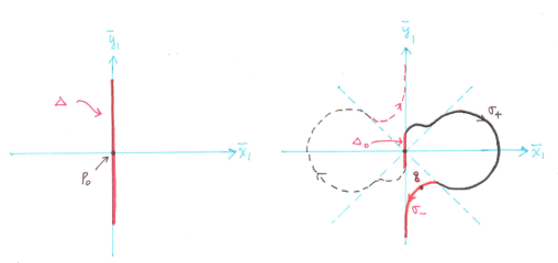
Figure 6: $\Delta$ before and after deformed.

The curves $\sigma_{\pm}$ are contained in the half plane $\{\bar{x}_{1}\geq 0\}$ in the $\bar{x}_{1}\bar{y}_{1}$ plane, and are oriented as in Figure 6. Write $\sigma:=\sigma_{+}\cup\sigma_{-}$. Following (24) the oriented Lagrangian locus $\check{\Gamma}_{0}^{+}\cap(\Delta\setminus\Delta_{0})$ is

(43) $$-\sigma\cup\tilde{g}_{\frac{\pi}{2}}(\sigma)\cup\tilde{g}_{\pi}(-\sigma)\cup\tilde{g}_{\frac{3\pi}{2}}(\sigma),$$

here $-\sigma$ means $\sigma$ but with the reversed orientation.

From now on we fix a reference point $q$ in the interior of $U_{-}$ as depicted in the right picture of Figure 6 so that $g^{\prime}_{L}$ is regular near $q$. $q$ is contained in a crossing domain of $L$ containing $\Delta$.

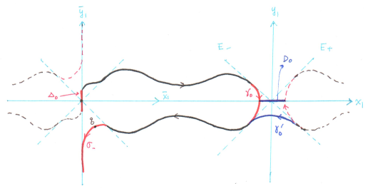
Figure 7: $\Delta$ for ”positive” surgery.

Next we apply another $\tilde{G}$-invariant Hamiltonian isotopy to $L$, keeping $L\setminus U_{+}$ fixed all the time, and turning $U_{+}$ to a new annulus also denoted as $U_{+}$, so that now $U_{+}$ contains a smaller annulus $U_{0}=Orb_{\tilde{G}}(\gamma_{0})$ as shown in Figure 7 such that

1. $U_{0}\subset T^{*}D_{\epsilon}$ is a crossing domain,

2. $\gamma_{0}$ is contained in the half plane $\{x_{1}<0\}$ in the $x_{1}y_{1}$-plane.

The loci $\check{\Gamma}^{+}_{s}$ together with their orientations are preserved under the $\tilde{G}$-invariant Hamiltonian isotopy. Then (43) implies that

$$\check{\Gamma}_{0}^{+}\cap U_{0}=(-\gamma_{0})\cup\tilde{g}_{\frac{\pi}{2}}(\gamma_{0})\cup\tilde{g}_{\pi}(-\gamma_{0})\cup\tilde{g}_{\frac{3\pi}{2}}(\gamma_{0}).$$

Recall that $E^{\prime}_{0}=\partial_{y_{1}}\wedge-\partial_{x_{1}}$ and $E^{\prime}_{\frac{\pi}{2}}=-\partial_{y_{2}}\wedge\partial_{x_{2}}$ along $-\gamma_{0}$. Since $(\Delta\varphi)_{-\gamma_{0}}=\pi$ (compare with Figure 5(b)) by applying (25) we have

$$\alpha_{0,U_{0}}=4(\Delta\varphi)_{-\gamma_{0}}=4\pi.$$

Observe that $D_{\epsilon}\subset S$ contains a smaller disk $D_{0}$ which is a $la$-disk of $L$ with $\partial D_{0}$ contained in the interior of $U_{0}$.

Apply $\eta_{D_{0}}$ to $L$ by replacing $U$ by a $\tilde{G}$-invariant Lagrangian annulus $U^{\prime}_{0}$ contained in a symplectic neighborhood of $D_{0}$ in $T^{*}S$ with $\partial U^{\prime}_{0}=\partial U_{0}$ to obtain a new smooth embedded Lagrangian surface

$$L^{1}=(L\setminus U_{0})\cup U^{\prime}_{0}.$$

Note that

$$L^{1}:=\eta_{D_{0}}(L)=\tau^{2}_{S}(L).$$

is also obtained by applying to $L$ a positive double Dehn twist with respect to $S$.

Write $U^{\prime}_{0}=Orb_{\tilde{G}}(\gamma^{\prime}_{0})$, where $\gamma^{\prime}_{0}$ is with the induced orientation and is contained the half plane $\{|x_{1}|<\epsilon,y_{1}<0\}$ as shown in Figure 7. For $L^{1}$, the Lagrangian locus $\check{\Gamma}^{+}_{0}$ restricted to $U_{1}$ is

$$\check{\Gamma}_{0}^{+}\cap U^{\prime}_{0}=(-\gamma^{\prime}_{0})\cup\tilde{g}_{\frac{\pi}{2}}(\gamma^{\prime}_{0})\cup\tilde{g}_{\pi}(-\gamma^{\prime}_{0})\cup\tilde{g}_{\frac{3\pi}{2}}(\gamma^{\prime}_{0}),$$

with $-\gamma^{\prime}_{0}$ denotes $\gamma^{\prime}_{0}$ but with the reversed orientation. We have $(\Delta\varphi)_{-\gamma^{\prime}_{0}}=-\pi$ and

$$\alpha_{0,U^{\prime}_{0}}=4(\Delta\varphi)_{-\gamma^{\prime}_{0}}=-4\pi.$$

Therefore

(44) $$\begin{split}y(L^{1},L,q;\EuFrak{f})&=y(L^{1},q;\EuFrak{f})-y(L,q;\EuFrak{f})\\ &=\frac{1}{2\pi}(\alpha_{0,U^{\prime}_{0}}-\alpha_{0,U_{0}})\\ &=\frac{1}{2\pi}(-4\pi-4\pi)\\ &=-4.\end{split}$$

Repeat similar Hamiltonian isotopies to $L^{1}$ so that $p_{0}$ and $L^{1}\setminus\Delta_{0}$ are fixed all the time, and the resulting $\Delta_{0}$ contains

• a smaller disk $\Delta_{1}\subset T^{*}_{p_{0}}S$, and

• an annular crossing domain $U_{1}\subset T^{*}D_{\epsilon}$ so that for $L^{1}$, the relative $E^{\prime}_{0}$-phase along $\check{\Gamma}^{+}_{0}\cap U_{1}$ is $\alpha_{0,U_{1}}=4\pi$, and

• there is a $la$-disk $D_{1}\subset D_{\epsilon}$ of $L^{1}$ with $\partial D_{1}$ contained in the the interior of $U_{1}$.

Apply $\eta_{D_{1}}$ to $L^{1}$ by replacing $U_{1}$ with another annular $U^{\prime}_{1}$ with $\partial U_{1}=\partial U^{\prime}_{1}$ we get a new Lagrangian surface

$$L^{2}=\eta_{D_{1}}(L^{1})=\tau^{2}_{S}(L^{1})=\tau^{4}_{S}(L)$$

which can also be obtained by applying $4$ positive generalized Dehn twists to $L$ along $S$. As in the case of $U^{\prime}_{0}$, the relative $E^{\prime}_{0}$-phase along $\check{\Gamma}_{0}^{+}\cap U^{\prime}_{1}$ is

$$\alpha_{0,U^{\prime}_{1}}=-4\pi.$$

So again we have

(45) $$\begin{split}y(L^{2},L^{1},q;\EuFrak{f})&=y(L^{2},q,\EuFrak{f})-y(L^{1},q;\EuFrak{f})\\ &=\frac{1}{2\pi}(\alpha_{0,U^{\prime}_{1}}-\alpha_{0,U_{1}})\\ &=\frac{1}{2\pi}(-4\pi-4\pi)\\ &=-4.\end{split}$$

Also it is easy to see that

(46) $$y(L^{2},L,q;\EuFrak{f})=-8.$$

Repeat this process to $(L^{k},\Delta_{k-1},\Delta_{k},U_{k},D_{k})$ to get $(L^{k+1},\Delta_{k},\Delta_{k+1},U_{k+1})$, and so on so forth, we obtain an infinite sequence of smoothly isotopic Lagrangian surfaces $L^{0}=L$, $L^{1}$, $L^{2}$,…, $L^{n}$,…, with $L^{n}=\tau^{2n}_{S}(L)$, and

(47) $$y(\tau^{2m}_{S}(L),\tau^{2n}_{S}(L),q;\EuFrak{f})=-4(m-n),\quad m,n\in\mathbb{N}\cup\{0\}.$$

Negative even Dehn twists.  Proceed to the case of double negative generalized Dehn twist. Again in $T^{*}\bar{D}$ we can deform $\Delta\subset L$ as in Figure 8 by a different $\tilde{G}$-invariant Hamiltonian isotopy in a neighborhood of $p_{0}\in W$, keeping $p_{0}$ and $L\setminus\Delta$ fixed all the time so that after the isotopy, $\Delta$ can be expressed as the union of three consecutive domains

$$\Delta=\Delta_{0}\cup U_{\dagger}\cup U_{-}$$

where $\Delta_{0}$ and $U_{-}$ are as before, $U_{\dagger}=Orb_{\tilde{G}}(\sigma_{\dagger})$ is a $p$-domain with PLG-degree $d_{U_{\dagger}}=-2$, $\sigma_{\dagger}$ is an oriented curve contained in the $\bar{x}_{1}\bar{y}_{1}$-plane as shown in Figure 8. We still use $q\in U_{-}$ as the reference point.

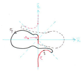
Figure 8: $\Delta$ deformed and before surgery.

Apply another $\tilde{G}$-invariant Hamiltonian isotopy to $L$, keeping $L\setminus U_{\dagger}$ fixed all the time, and turning $U_{\dagger}$ to a new annulus also denoted as $U_{\dagger}$, so that now $U_{\dagger}$ contains $-U_{0}$ which denotes the crossing domain $U_{0}$ but with the reversed orientation, as shown in Figure 9. We can write $-U_{0}=Orb_{\tilde{G}}(-\bar{\gamma}_{0})$ where

$$-\bar{\gamma}_{0}:=\tilde{g}_{\pi}(-\gamma)$$

is a curve contained in the half plane $\{0<x_{1}<\epsilon\}$ in the $x_{1}y_{1}$-plane.

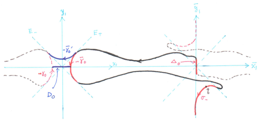
Figure 9: $\Delta$ and $D_{0}$ for ”negative” surgery.

We have

$$\check{\Gamma}_{0}^{+}\cap-U_{0}=\gamma_{0}\cup\tilde{g}_{\frac{\pi}{2}}(-\gamma_{0})\cup\tilde{g}_{\pi}(\gamma_{0})\cup\tilde{g}_{\frac{3\pi}{2}}(-\gamma_{0}).$$

Since $(\Delta\varphi)_{\gamma_{0}}=-\pi$ we have

$$\alpha_{0,-U_{0}}=4(\Delta\varphi)_{\gamma_{0}}=-4\pi.$$

Recall $D_{\epsilon}\subset S$ contains a smaller disk $D_{0}$ which is a $la$-disk of $L$ with $\partial D_{0}$ contained in the interior of $U^{-}_{0}$.

Apply $\eta_{D_{0}}$ to $L$ by replacing $-U_{0}$ by a $\tilde{G}$-invariant Lagrangian annulus $-U^{\prime}_{0}$, the annulus $U^{\prime}_{0}$ with the reversed orientation, contained in a symplectic neighborhood of $D_{0}$ in $T^{*}S$ with $\partial(-U^{\prime}_{0})=\partial(-U_{0})$ to obtain a new smooth embedded Lagrangian surface

$$L^{-1}:=(L\setminus(-U_{0}))\cup(-U^{\prime}_{0}).$$

Note that

$$L^{-1}=\eta_{D_{0}}(L)=\tau^{-2}_{S}(L).$$

is also obtained by applying to $L$ a negative double Dehn twist with respect to $S$.

Like the case for $-U_{0}$, we can write $-U^{\prime}_{0}=Orb_{\tilde{G}}(-\gamma^{\prime}_{0})$, where $-\gamma^{\prime}_{0}$ is $\gamma^{\prime}_{0}$ but with the reversed orientation as shown in Figure 9. For $L^{-1}$, the Lagrangian locus $\check{\Gamma}^{+}_{0}$ restricted to $-U^{\prime}_{0}$ is

$$\check{\Gamma}_{0}^{+}\cap(-U^{\prime}_{0})=\gamma^{\prime}_{0}\cup\tilde{g}_{\frac{\pi}{2}}(-\gamma^{\prime}_{0})\cup\tilde{g}_{\pi}(\gamma^{\prime}_{0})\cup\tilde{g}_{\frac{3\pi}{2}}(-\gamma^{\prime}_{0}).$$

As $(\Delta\varphi)_{\gamma^{\prime}_{0}}=\pi$ it follows that

$$\alpha_{0,-U^{\prime}_{0}}=4(\Delta\varphi)_{\gamma^{\prime}_{0}}=4\pi.$$

Therefore

(48) $$\begin{split}y(L^{-1},L,q;\EuFrak{f})&=y(L^{-1},q,\EuFrak{f})-y(L,q;\EuFrak{f})\\ &=\frac{1}{2\pi}(\alpha_{0,-U^{\prime}_{0}}-\alpha_{0,-U_{0}})\\ &=\frac{1}{2\pi}(4\pi+(-4\pi))\\ &=4.\end{split}$$

Apply to $(L^{-1},\Delta_{0})$ $\tilde{G}$-invariant Hamiltonian isotopies similar to those applied to $(L,\Delta)$ we get $(L^{-1},\Delta_{0},\Delta_{1},-U_{1},D_{1})$ with $\Delta_{1}\cup(-U_{1})\subset\Delta_{0}$. Then apply $\eta_{D_{1}}$ to get $L^{-2}=\tau^{-2}_{S}(L^{-1})=\tau^{-4}_{S}(L)$, and so on so forth, we obtain an infinite sequence $(L^{-n},\Delta_{n-1},\Delta_{n},-U_{n},D_{n})$, $n\in\mathbb{N}$, with $L^{-n}=\tau^{-2n}_{S}(L)$, and

(49) $$y(\tau^{-2m}_{S}(L),\tau^{-2n}_{S}(L),q;\EuFrak{f})=4(m-n),\quad m,n\in\mathbb{N}\cup\{0\}.$$

Summing up the results for positive and negative even Dehn twists, we arrive at the following conclusion:

Proposition 5.3.1.

Assume that an orientable Lagrangian surface $L$ intersects transversally with a Lagrangian sphere $S$ and in a point $p$. Let $L^{n}:=\tau^{2n}_{S}(L)$ for $n\in\mathbb{Z}$. Then

$$y(L^{n},L^{m},q;\EuFrak{f})=4(m-n),m,n\in\mathbb{Z}.$$

$$y(L^{n},L,q;\EuFrak{f})=-4n,\quad n\in\mathbb{Z}.$$

5.4 Monotone tori in $W_{n}$

Recall for any integer $n\geq 1$ the Stein surface $W_{n}\subset\mathbb{C}^{3}$ defined by the equation

$$z_{1}^{2}+z_{2}^{2}=z_{3}^{n+1}+\frac{1}{2}.$$

$W_{n}$ is the plumbing of $n$ copies of $T^{*}S^{2}$ so that the Lagrangian zero-section spheres $S_{1}$,…,$S_{n}$ form an $A_{n}$-configuration: $S_{j}\pitchfork S_{j+1}$ and in one point, $S_{i}\cap S_{j}=\emptyset$ if $|i-j|\neq 1$. Each of $W_{n}$ is a parallelizable symplectic 4-manifold, and its unitary framing is unique up to homotopy.

To facilitate later computation we identify for each $k$ $S_{k}=D_{k}\cup_{\psi_{k}}\bar{D}_{k}$, where $D_{k}:=\{x^{k}=(x^{k}_{1},x^{k}_{2})\in\mathbb{R}^{2}\mid|x^{k}|\leq 1\}$, $\bar{D}_{k}:=\{\bar{x}^{k}=(\bar{x}^{k}_{1},\bar{x}^{k}_{2})\in\mathbb{R}^{2}\mid|\bar{x}^{k}|\leq 1\}$, and $\psi_{k}:\bar{D}_{k}-\{0\}\to D_{k}-\{0\}$ a diffeomorphism defined similar to $\psi$ as in (27). Let $T^{*,\epsilon}D_{k}$ denote the cotangent disk bundle of $D_{k}$ with fiber coordinates $y^{k}=(y^{k}_{1},y^{k}_{2})$, $|y^{k}|<\epsilon$. Similarly $T^{*,\epsilon}\bar{D}_{k}$ denotes the cotangent disk bundle of $\bar{D}_{k}$ with fiber coordinates $\bar{y}^{k}=(\bar{y}^{k}_{1},\bar{y}^{k}_{2})$, $|\bar{y}^{k}|<\epsilon$. Here $\epsilon>0$ is some fixed small number. Then $\psi_{k}$ induces a symplectic diffeomorphism $\Psi_{k}:T^{*,\epsilon}(\bar{D}\setminus\{0\})\to T^{*,\epsilon}(D\setminus\{0\})$. We consider for $k=2,3,...n$ plumbings

$$\chi_{k}:T^{*,\epsilon}(\{|\bar{x}^{k}|<\epsilon\})\to T^{*,\epsilon}(\{|x^{k-1}|<\epsilon\})$$

defined by the following identifications

$$\bar{x}^{k}_{1}\ \longleftrightarrow\ y^{k-1}_{1}$$

$$\bar{x}^{k}_{2}\ \longleftrightarrow\ -y^{k-1}_{2}$$

$$\bar{y}^{k}_{1}\ \longleftrightarrow\ -x^{k-1}_{1}$$

$$\bar{y}^{k}_{2}\ \longleftrightarrow\ x^{k-1}_{2}$$

The resulting manifold is $W_{n}$.

Identify $T^{*,\epsilon}D_{k}$ as complex domains in $\mathbb{C}^{2}$ with complex coordinates $z^{k}_{j}:=x^{k}_{j}+\sqrt{-1}y^{k}_{j}$, and $T^{*,\epsilon}\bar{D}_{k}$ as complex domains in $\mathbb{C}^{2}$ with complex coordinates $w^{k}_{j}:=\bar{x}^{k}_{j}+\sqrt{-1}\bar{y}^{k}_{j}$. Then both $\Psi_{k}$ and $\chi_{k}$ are holomorphic and $\tilde{G}$-invariant where $\tilde{G}$ is an $S^{1}$-group acting on $T^{*,\epsilon}\bar{D}_{k}$ as counterclockwise rotations

$$\begin{pmatrix}\cos\theta&-\sin\theta\\ \sin\theta&\cos\theta\end{pmatrix}$$

with respect to the complex coordinates $(w^{k}_{1},w^{k}_{2})$, and acting on $T^{*,\epsilon}D_{k}$ as clockwise rotations

$$\begin{pmatrix}\cos\theta&\sin\theta\\ -\sin\theta&\cos\theta\end{pmatrix}$$

with respect to the complex coordinates $(z^{k}_{1},z^{k}_{2})$,

We fix a unitary basis $(u,v)$ on $W_{n}$ so that on each $T^{*,\epsilon}S_{k}$ it is the unitary basis on $T^{*}S$ as used in Section 5.3,

$$(u,v)=\begin{cases}(\partial_{\bar{x}^{k}_{1}},\partial_{\bar{x}^{k}_{2}})&\text{ on $\{|\bar{x}^{k}|<\epsilon,\ |\bar{y}^{k}|<\epsilon\}$},\\ (\partial_{y^{k}_{1}},-\partial_{y^{k}_{2}})&\text{ on $\{|x^{k}|<\epsilon,\ |y^{k}|<\epsilon\}$}.\end{cases}$$

Let $E^{\prime}_{s}$, $s\in\mathbb{R}/\pi\mathbb{Z}$ denote the $S^{1}$-family of complex line bundles associated to $(u,v)$,

$$E^{\prime}_{s}=\begin{cases}(\cos s\partial_{\bar{x}^{k}_{1}}+\sin s\partial_{\bar{x}^{k}_{2}})\wedge(\cos s\partial_{\bar{y}^{k}_{1}}+\sin s\partial_{\bar{y}^{k}_{2}})&\text{ on $T^{*,\epsilon}\bar{D}_{k}$},\\ (\cos s\partial_{y^{k}_{1}}-\sin s\partial_{y^{k}_{2}})\wedge(-\cos s\partial_{x^{k}_{1}}+\sin s\partial_{x^{k}_{2}})&\text{ on $T^{*,\epsilon}D_{k}$}\end{cases}$$

Let $C^{k}_{0},C^{k}_{\frac{\pi}{2}}$ be the equators of $S_{k}$ defined by $C^{k}_{0}:=\{x_{2}=0\}\cup\{\bar{x}_{2}=0\}$, $C^{k}_{\frac{\pi}{2}}:=\{x_{1}=0\}\cup\{\bar{x}_{1}=0\}$. Then similar to the corresponding case in Section 5.3 we have that $E^{\prime}_{0}$ is tangent to $\cup_{k=1}^{n}T^{*}C^{k}_{0}$ and orthogonal to $\cup_{k=1}^{n}T^{*}C^{k}_{\frac{\pi}{2}}$, $E^{\prime}_{\frac{\pi}{2}}$ is tangent to $\cup_{k=1}^{n}T^{*}C^{k}_{\frac{\pi}{2}}$ and orthogonal to $\cup_{k=1}^{n}T^{*}C^{k}_{0}$.

Let $T_{-1}\subset\{|\bar{x}^{1}|<\epsilon,|\bar{y}^{1}|<\epsilon\}\subset T^{*,\epsilon}S_{1}$ be the (Chekanov) torus defined as the $\tilde{G}$ orbit of the circle $\upsilon=\sigma\cup\gamma_{-1}\subset\{\bar{y}^{1}_{1}>0\}\cap\Sigma_{0}$ (see Figure 10),

(50) $$\sigma(s) :=(\bar{x}^{1}_{1}=-r\sin s,\ \bar{y}^{1}_{1}=\sqrt{2}r+r\cos s),\quad\frac{-3\pi}{4}\leq s\leq\frac{3\pi}{4},$$

(51) $$\gamma_{-1}(s) :=(\bar{x}^{1}_{1}=-r\sin s,\ \bar{y}^{1}_{1}=\sqrt{2}r+r\cos s),\quad\frac{3\pi}{4}\leq s\leq\frac{5\pi}{4}.$$

Orient $T_{-1}$ so that $\{\dot{\upsilon},\tilde{X}(\upsilon)\}$ is a positive basis of $T_{\upsilon}(T_{-1})$. $U_{\sigma}:=Orb_{\tilde{G}}(\sigma)$ and $U_{-1}:=Orb_{\tilde{G}}(\gamma_{-1})$ are crossing domains of $T_{-1}$. Fix a regular interior point $q$ of $U_{\sigma}$ as the reference point.

The oriented proper $E^{\prime}_{0}$-locus of $T_{-1}$ is

$$\check{\Gamma}^{\prime}_{0}=\upsilon\cup\tilde{g}_{\frac{\pi}{2}}(-\upsilon)\cup\tilde{g}_{\pi}(\upsilon)\cup\tilde{g}_{\frac{3\pi}{2}}(-\upsilon).$$

We have

$$(\Delta\varphi)_{\sigma}=\pi,\quad(\Delta\varphi)_{\gamma_{-1}}=\pi,$$

(52) $$y(T_{-1},q)=\frac{1}{2\pi}(4(\Delta\varphi)_{\sigma}+4(\Delta\varphi)_{\gamma_{-1}})=\frac{1}{2\pi}(4\pi+4\pi)=4.$$

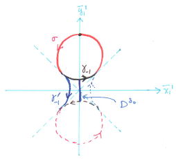
Figure 10: From $T_{-1}$ to $T_{0}$.

The disk fiber $T^{*,\epsilon}_{p_{0}}(\bar{D}_{1})$ contains a stable $la$-disk $D^{\delta_{0}}$ of $T_{-1}$ with its boundary lies in the interior of $U_{-1}$ (see Figure 10). Let $\gamma^{\prime}_{-1}:=M(\gamma_{-1})$, and $U^{\prime}_{-1}:=Orb_{\tilde{G}}(\gamma^{\prime}_{-1})$. Let $T_{0}=\eta_{D^{\delta_{0}}}(T_{-1})$ denote the Lagrangian torus obtained by replacing $U_{-1}$ by $U^{\prime}_{-1}$:

$$T_{0}=U_{\sigma}\cup U^{\prime}_{-1}.$$

Observe that $(\Delta\varphi)_{\gamma^{\prime}_{-1}}=-\pi$, so

(53) $$y(T_{0},q)=\frac{1}{2\pi}(4(\Delta\varphi)_{\sigma}+4(\Delta\varphi)_{\gamma^{\prime}_{-1}})=0,$$

(54) $$\begin{split}y(T_{0},T_{-1},q)&:=y(T_{0},q)-y(T_{-1},q)\\ &=\frac{1}{2\pi}(4(\Delta\varphi)_{\gamma^{\prime}_{-1}}-4(\Delta\varphi)_{\gamma_{-1}})\\ &=-4.\end{split}$$

Figure 11: From $T_{0}$ to $T_{1}$.

With a $\tilde{G}$-invariant Hamiltonian isotopy with $U_{\sigma}$ kept fixed all the time we may deform $U^{\prime}_{-1}$ to a new Lagrangian annulus, also denoted as $U^{\prime}_{-1}$, so that the deformed $\gamma^{\prime}_{-1}$ contains an arc $\gamma_{0}$ lying in $(T^{*,\epsilon}D_{1})\cap\{x^{1}_{2}=0=y^{1}_{2}\}$ as shown in Figure 11, so that $U_{0}:=Orb_{\tilde{G}}(\gamma_{0})$ is a crossing domain and

$$(\Delta\varphi)_{\gamma_{0}}=\pi.$$

For example we may take $\gamma_{0}$ to be the oriented arc

$$\gamma_{0}(s)=(x^{1}_{1}=-\sqrt{2}r_{1}-r_{1}\cos s,y^{1}_{1}=-r_{1}\sin s),\quad\frac{3\pi}{4}\leq s\leq\frac{5\pi}{4}.$$

Observe that $D_{1}$ contains a stable $la$-disk $D^{\delta_{1}}$ of $T_{0}$ with its boundary lying in the interior of $U_{0}$. Let $\gamma^{\prime}_{0}:=M(\gamma_{0})$, then similar to the case of the pair $(\gamma_{-1},\gamma^{\prime}_{-1}:=M(\gamma_{-1}))$ we have

$$(\Delta\varphi)_{\gamma^{\prime}_{0}}=-\pi=-(\Delta\varphi)_{\gamma_{0}}.$$

Let $T_{1}:=\eta_{D^{\delta_{1}}}$ denote the Lagrangian torus obtained from $T_{0}$ by replacing $U_{0}$ by $U^{\prime}_{0}$:

$$T_{1}:=(T_{0}\setminus U_{0})\cup U^{\prime}_{0}.$$

Then similar to the case for $T_{-1}$ and $T_{0}=\eta_{D^{\delta_{0}}}(T_{-1})$, we have

(55) $$y(T_{1},T_{0},q)=\frac{1}{2\pi}(4(\Delta\varphi)_{\gamma^{\prime}_{0}}-4(\Delta\varphi)_{\gamma_{0}})=\frac{1}{2\pi}(-4\pi-4\pi)=-4,$$

and

(56) $$y(T_{1},q)=y(T_{1},T_{0},q)+y(T_{0},q)=-4+0=-4,$$

(57) $$y(T_{1},T_{-1},q)=-8.$$

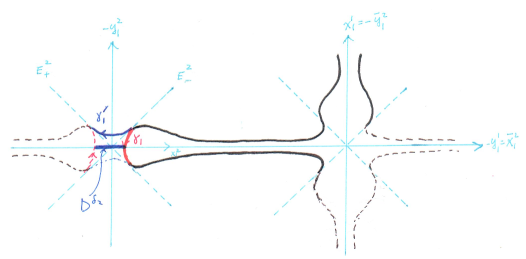
Figure 12: From $T_{1}$ to $T_{2}$.

Now starting from $k=1$ repeat the above procedure successively for $k=1,...,n-1$ to get a sequence of monotone Lagrangian tori $T_{k}$ by a sequence of $la$-disk surgeries as follows:

1. Hamiltonian isotop $U^{\prime}_{k-1}$ rel $\partial U^{\prime}_{k-1}$ of $T_{k}$ in a $\tilde{G}$-invariant fashion so that after the isotopy the interior of $U^{\prime}_{k-1}$ contains a crossing domain $U_{k}:=Orb_{\tilde{G}}(\gamma_{k})$ with $(\Delta\varphi)_{\gamma_{k}}=\pi$.

2. Apply $la$-disk surgery to $T_{k}$ to get

   $$T_{k+1}:=(T_{k}\setminus U_{k})\cup U^{\prime}_{k}$$

   where

   $$U^{\prime}_{k}=Orb_{\tilde{G}}(\gamma^{\prime}_{k}),\quad\gamma^{\prime}_{k}=M(\gamma_{k}),$$

   and $(\Delta\varphi)_{\gamma^{\prime}_{k}}=-\pi$.

Note that all of $T_{k}$ are smoothly isotopic and contain the domain $U_{\sigma}$. Then

(58) $$y(T_{k+1},T_{k},q)=\frac{1}{2\pi}(4(\Delta\varphi)_{\gamma^{\prime}_{k}}-4(\Delta\varphi)_{\gamma_{k}})=-4,$$

hence

(59) $$y(T_{k},q)=-4k,\quad k=-1,0,1,...,n,$$

and

(60) $$y(T_{k},T_{j},q)=4(j-k),\quad-1\leq k,j\leq n.$$

So $T_{k}$, $k=-1,0,1,...,n$, are pairwise non-Hamiltonian isotopic in $W_{n}$.

References

- [1] P. Albers, U. Frauenfelder, A nondisplaceable Lagrangian torus in , Comm. Pure Appl. Math. 61 (2008), no. 8, 1046–1051.
- [2] D. Auroux, Mirror symmetry and T-duality in the complement of an anticanonical divisor. J. G kova Geom. Topol. GGT 1 (2007), 51–91.
- [3] L. Bates, Monodromy in the champagne bottle, Z. Angew. Math. Phys. 42 (1991), no. 6, 837–847.
- [4] Y. V. Chekanov, Lagrangian tori in a symplectic vector space and global symplectomorphisms, Math. Z. 223 (1996), no. 4, 547–559.
- [5] J. J. Duistermaat, On global action-angle coordinates, Comm. Pure Appl. Math. 33 (1980), no. 6, 687–706.
- [6] I. Ekeland, H. Hofer, Symplectic topology and Hamiltonian dynamics. Math. Z. 200 (1989), no. 3, 355–378.
- [7] I. Ekeland, H. Hofer, Symplectic topology and Hamiltonian dynamics. II. Math. Z. 203 (1990), no. 4, 553–567.
- [8] Y. Eliashberg, Topological characterization of Stein manifolds of dimension , Internat. J. Math. 1 (1990), no. 1, 29–46.
- [9] Y. Eliashberg, L. Polterovich, The problem of Lagrangian knots in four-manifolds. Geometric topology (Athens, GA, 1993), 313–327, AMS/IP Stud. Adv. Math., 2.1, Amer. Math. Soc., Providence, RI, 1997.
- [10] R. Hind, Lagrangian spheres in . Geom. Funct. Anal. 14 (2004), no. 2, 303–318.
- [11] R. Hind, Lagrangian unknottedness in Stein surfaces. Asian J. Math. 16 (2012), no. 1, 1–36. .
- [12] M. Khovanov and P. Seidel, Quivers, Floer cohomology, and braid group actions, J. Amer. Math. Soc. 15 (2002), no. 1, 203 271.
- [13] A. Knapp, Lagrangian tori in closed 4-manifolds, J. Topol. 3 (2010), no. 2, 333 342.
- [14] D. McDuff and D. Salamon, Introduction to Symplectic Topology, 2nd ed., Oxford Mathematical Monographs, 1998.
- [15] Y.-G. Oh, Floer cohomology of Lagrangian intersections and pseudo-holomorphic disks, I, Comm. Pure Appl. Math. 46 (1993), no. 7, 949 993.
- [16] Y.-G. Oh, Addendum to ”Floer cohomology of Lagrangian intersections and pseudo-holomorphic disks, I”, Comm. Pure Appl. Math. 48 (1995), no. 11, 1299 1302.
- [17] L. Polterovich, The surgery of Lagrange submanifolds, Geom. Funct. Anal. 1 (1991), no. 2, 198–210.
- [18] M. Poźniak, Floer homology, Novikov rings and clean intersections. Northern California Symplectic Geometry Seminar, 119–181, Amer. Math. Soc. Transl. Ser. 2, 196, Amer. Math. Soc., Providence, RI, 1999.
- [19] P. Seidel, Lagrangian two-spheres can be symplectically knotted, J. Diff. Geom. 52 (1999) no. 1, 145–171.
- [20] A. Weinstein, Lectures on symplectic manifolds. Corrected reprint. CBMS Regional Conference Series in Mathematics, 29. American Mathematical Society, Providence, R.I., 1979.
- [21] C. Viterbo, Capacités symplectiques et applications (d’aprés Ekeland-Hofer, Gromov). (French) [Symplectic capacities and applications (after Ekeland-Hofer, Gromov)] Séminaire Bourbaki, Vol. 1988/89. Ast risque No. 177-178 (1989), Exp. No. 714, 345–362.
- [22] C. Viterbo, Plongements lagrangiens et capacités symplectiques de tores dans . (French) [The symplectic capacity of Lagrangian tori in R2n] C. R. Acad. Sci. Paris Sér. I Math. 311 (1990), no. 8, 487 490.
- [23] M.-L. Yau, Monodromy and isotopy of monotone Lagrangian tori, Math. Res. Lett. Vol. 16, Issue 3 (2009), 531–541. Department of Mathematics, National Central University, Chung-Li, Taiwan. Email address: yau@math.ncu.edu.tw