INTERSTELLAR H₂O MASERS FROM J SHOCKS

Abstract

We present a model in which the 22 GHz H₂O masers observed in star-forming regions occur behind shocks propagating in dense regions (preshock density $n_{0}$ $\sim$ $10^{6}$–$10^{8}$ cm^-3). We focus on high-velocity ($v_{s}\,\raise 1.29167pt\hbox{$>$}\kern-7.5pt\lower 3.01385pt\hbox{$\sim$}\,30$ km s^-1) dissociative J shocks in which the heat of H₂ re-formation maintains a large column of $\sim$ 300–400 K gas; at these temperatures the chemistry drives a considerable fraction of the oxygen not in CO to form H₂O. The H₂O column densities, the hydrogen densities, and the warm temperatures produced by these shocks are sufficiently high to enable powerful maser action. The observed brightness temperatures (generally $\sim$ $10^{11}$–$10^{14}$ K) are the result of coherent velocity regions that have dimensions in the shock plane that are 10 to 100 times the shock thickness of $\sim 10^{13}$ cm. The masers are therefore beamed towards the observer, who typically views the shock “edge-on”, or perpendicular to the shock velocity; the brightest masers are then observed with the lowest line of sight velocities with respect to the ambient gas. We present numerical and analytic studies of the dependence of the maser inversion, the resultant brightness temperature, the maser spot size and shape, the isotropic luminosity, and the maser region magnetic field on the shock parameters and the coherence path length; the overall result is that in galactic H₂O 22 GHz masers these observed parameters can be produced in J shocks with $n_{0}\sim$ $10^{6}$–$10^{8}$ cm^-3 and $v_{s}\sim 30$ –$200$ km s^-1. A number of key observables such as maser shape, brightness temperature, and global isotropic luminosity depend only on the particle flux into the shock, $j=n_{0}v_{s}$, rather than on $n_{0}$ and $v_{s}$ separately.

1 Introduction

Interstellar H₂O 22 GHz masers are associated with the earliest, most embedded, phases of both low-mass and high-mass star formation, once the strong protostellar outflows have commenced. In the low-mass case, Furuya et al (2001, 2003) find that while there are no masers in pre-protostellar cores, all class 0 protostars likely have water masers, with a lower fraction in class I and none in class II. These masers often appear to be individual clumps, streaming away from some center of activity at velocities up to 200 km s^-1. Individual features have apparent sizes of $\sim 10^{13}-10^{14}$ cm (Genzel 1986; Gwinn 1994a; Torrelles et al 2001a,b; Lekht et al 2007; Marvel et al 2008) and brightness temperatures usually in the range $T_{b}\sim 10^{11}-10^{14}$ K (Genzel 1986, Gwinn 1994b). The brightness of the masers suggests they are saturated and their observed linewidths ($\,\raise 1.29167pt\hbox{$<$}\kern-7.5pt\lower 3.01385pt\hbox{$\sim$}\,1$ km s^-1) suggest thermal temperatures generally $\,\raise 1.29167pt\hbox{$<$}\kern-7.5pt\lower 3.01385pt\hbox{$\sim$}\,1000$ K (Liljestrom & Gwinn 2000). The isotropic luminosity of individual maser spots ranges from $\,\raise 1.29167pt\hbox{$<$}\kern-7.5pt\lower 3.01385pt\hbox{$\sim$}\,10^{-6}$ to 0.08 $L_{\odot}$ in the Galaxy (Walker, Matsakis & Garcia-Barreto 1982, Gwinn 1994a). The individual maser spots are highly beamed toward the observer (Gwinn 1994c), so that the observed flux of an individual spot measures an (assumed) isotropic luminosity that is much higher than its actual luminosity. Pumping by an external source of radiation is ruled out by observations (e.g., Genzel 1986), and an internal source of pump energy, such as the thermal energy produced in a shock, seems required.

The development of powerful shocks in maser regions is inevitable in light of the high velocities observed in the sources; Gwinn (1994a), Claussen et al (1998), and Liljestrom & Gwinn (2000) show, for example, that the vast majority of maser spots in W49 and IRAS 05413-0104 have space velocities in excess of 25 km s^-1. The H₂O maser luminosity correlates with the mechanical luminosity in the observed outflows or in the protostellar jets (Felli, Palagi & Tofani 1992, Claussen et al 1996, Furuya et al 2001), as would be expected in a shock model. The source of excitation, then, appears to be the interaction of the powerful outflows or jets from protostars in their earliest, most embedded, phases of evolution with the dense gas that surrounds them in this early stage — either gas in disks or gas in the dense envelopes that surround protostar/disk systems. Recent high angular resolution and proper motion studies indicate groups of maser spots expanding away from the exciting source, a geometry and dynamics highly suggestive of shocks (Gwinn 1994a; Torrelles et al 2001a,b; Lekht et al 2007; Marvel et al 2008; Goddi et al 2011; Moscadelli et al 2013). In particular, the velocity vectors that Marvel et al find in several sources are in close agreement with propagation in the plane of the sky, as expected in shock-excited masers. The observed fluxes from the maser spots in W49N that are within 10 km s^-1 of the systemic radial velocity can be up to an order of magnitude greater than those from spots outside this velocity range (Liljestrom & Gwinn 2000), which again is consistent with excitation by shocks propagating perpendicular to the line of sight. Further evidence comes from a recent survey by Walsh et al (2011), which finds that although maser emission is spread over 350 km s^-1, 90% of maser sites have a velocity spread of less than 50 km s^-1. The high-resolution observations of W49 and W3OH show that the maser features outline the surfaces of elongated cocoons whose expansion is driven by twin high-velocity ($\sim$ 1000 km s^-1), very young (a few hundred years) jets (Elitzur 1995). In low-mass star-forming regions the ambient density can be expected to be lower and the jets penetrate without creating complete shells, leading to H-H objects and maser action only on working surfaces where they generate local shocks. H₂O maser emission is also seen associated with jets and their interaction with slower moving material around AGB stars (Imai et al 2002) and planetary nebulae (Miranda et al 2001, Uscanga et al 2008). Recently, a new class of six “water fountain” pre-planetary nebulae have been found which display bipolar structure with maser arcs aligned with high velocity outflows (Claussen et al 2009, Day et al 2010). Finally, very strong H₂O maser emission is observed in extragalactic sources where shocks may be implicated such as the disks orbiting AGNs (Maoz & McKee 1998 and references therein), the jets from AGNs (Peck et al 2003, Tarchi et al 2011), and in nearby star-forming galaxies (Darling et al 2008, Brogan et al 2010, Imai et al 2013).

Several authors besides ourselves have theoretically treated the possibility of a shock origin for interstellar H₂O masers (Strelnitski 1973, 1980, 1984; Schmeld, Strelnitski & Muzylev 1976; Kylafis & Norman 1986; Tarter & Welch 1986). However, these models either lacked detail, required huge preshock hydrogen densities ($>10^{9}$ cm^-3) and therefore severe energy requirements, or posited physically implausible electron and neutral temperatures. We (Hollenbach, McKee & Chernoff 1987, Elitzur, Hollenbach & McKee 1989, hereafter EHM, and Hollenbach, Elitzur & McKee 1993) have proposed a detailed shock model with calculated temperature and chemical structures and with much less severe energy requirements. In our model the preshock gas has hydrogen densities $n_{0}\,\raise 1.29167pt\hbox{$>$}\kern-7.5pt\lower 3.01385pt\hbox{$\sim$}\,10^{6}$ cm^-3 and the masing occurs in postshock gas with densities $n_{p}\sim 10^{8}-10^{9}$ cm^-3. One of our key realizations was that the re-formation of molecular hydrogen in the postshock gas provided a heating source that was essential in dissociative J shocks in order to produce the columns of warm H₂O needed for observable interstellar masers. Our work has focussed on fast ($v_{s}\,\raise 1.29167pt\hbox{$>$}\kern-7.5pt\lower 3.01385pt\hbox{$\sim$}\,30-50$ km s^-1) dissociative J shocks [see Draine (1980) for original definitions of J and C shocks], but we have noted (EHM; Elitzur, Hollenbach, & McKee 1992, hereafter EHM92) that non-dissociative C shocks may also produce masers. Such shocks are limited to velocities of $\,\raise 1.29167pt\hbox{$<$}\kern-7.5pt\lower 3.01385pt\hbox{$\sim$}\,40$ km s^-1 set by runaway ionization when relative velocity between neutrals and ions in the shock becomes too large (Draine & McKee 1993; Flower & Pineau des Forêts 2010). Just as in our J-shock models, in these C shocks the H₂O is collisionally excited by warm neutral particles (H and H₂) and the escaping H₂O infrared line radiation creates the inversions. Kaufman & Neufeld (1996) have modeled H₂O maser emission from such C shocks, and applied their results to observations of 22 GHz and of other H₂O maser transitions, especially in the submillimeter wavelength region (Menten, Melnick, & Phillips 1990; Cernicharo et al 1990; Menten et al 1990; Melnick et al 1993). Detailed pumping calculations by Yates et al (1997) show that the 22 GHz masers have a broader range of physical conditions than the submillimeter masers. According to these models there can be 22 GHz emission and no accompanying 321 GHz masers in the same region, but not vice versa. Significant submillimeter maser radiation requires emission regions at high temperatures ($\,\raise 1.29167pt\hbox{$>$}\kern-7.5pt\lower 3.01385pt\hbox{$\sim$}\,1000$ K) that are more readily produced behind C shocks.

Because of observational challenges, the submillimeter masers have remained relatively unstudied. Only recently, Patel et al (2007) imaged for the first time the 321 GHz maser with the Submillimeter Array (SMA) in the Cepheus A high-mass star-forming region, where they also mapped the 22 GHZ maser with the Very Large Array (VLA). Nine submillimeter maser spots were detected and three of them are associated with the centimeter masers spatially as well as kinematically. In addition, there are 36 22 GHz maser spots without corresponding submillimeter masers. These observations indicate that the submillimeter masers are tracing significantly hotter regions (600–2000 K) than the centimeter masers; 22 GHz masers that are not associated with the 321 GHz masers are likely to be arising in relatively cooler regions.

Overwhelmingly, the 22 GHz maser remains the most widely studied transition of water, and in this paper we treat its production by J shocks. EHM demonstrated numerically that J shocks with $n_{0}=10^{7}$ cm^-3, $v_{s}=100$ km s^-1 produce bright H₂O masers and gave analytic formulae for the dependence of maser parameters on the shock parameters. This paper extends that work by providing a numerical study of the range of J shocks that produce H₂O masers. We show that shocks in the range 10⁶ cm${}^{-3}\,\raise 1.29167pt\hbox{$<$}\kern-7.5pt\lower 3.01385pt\hbox{$\sim$}\,n_{0}\,\raise 1.29167pt\hbox{$<$}\kern-7.5pt\lower 3.01385pt\hbox{$\sim$}\,10^{8}$ cm^-3 and 30 km s${}^{-1}\,\raise 1.29167pt\hbox{$<$}\kern-7.5pt\lower 3.01385pt\hbox{$\sim$}\,v_{s}\,\raise 1.29167pt\hbox{$<$}\kern-7.5pt\lower 3.01385pt\hbox{$\sim$}\,200$ km s^-1 are likely to produce the observed fast interstellar 22 GHz H₂O masers. EHM noted that this model could apply to powerful extragalactic masers as well, and Maoz & McKee (1998) developed a detailed model for circumnuclear masers. In §2 we model the H₂O level populations and the radiative transfer of the H₂O transitions in an isothermal and isochoric slab such as is produced in dense, fast J shocks, and we present analytic scalings and numerical results. In §3 we describe the physics incorporated into the shock code and present analytic and numerical results for the shock structure. In §4 we apply the H₂O maser slab results to the shock models in order to predict the 22 GHz brightness temperature $T_{b}$ of a single maser spot, its isotropic luminosity $L_{\rm iso}$, and the shape and size of the maser spot as functions of the physical parameters $n_{0}$, $v_{s}$, $v_{A}$ (the preshock Alfven speed – a measure of the preshock magnetic field), and the coherence pathlength $2\ell$ in the shock plane. We also discuss the overall luminosity from a shocked masing region composed of many maser spots (§4.3). We compare the J-shock and C-shock masers in §4.4. In §5, we summarize our conclusions.

2 H₂O MASER SLAB MODELS

Fast, dense, dissociative J shocks produce a planar H₂ re-formation plateau region that is nearly isothermal and isochoric. Here we model the H₂O maser emission from a planar homogenous slab, deriving results applicable to all collisionally pumped slabs, including C shocks, that may produce H₂O maser emission (EHM; EHM92; Kaufman & Neufeld 1996). These results are combined with J-shock models in §4.

A reasonably accurate description of maser emission under all circumstances is provided by a standard formalism (see, e.g., Elitzur 1992; E92 hereafter) whose essentials we reproduce in Appendix A for completeness. In this formalism the maser system is characterized by spatially constant effective pump and loss rates that describe the interactions with all other levels, which constitute the maser reservoir. The pump and loss rates are obtained from a solution of the level populations for the full system (maser and reservoir) in the absence of maser radiation (the unsaturated limit). We start with this calculation, proceed to derive the parameters of the ${\rm H_{2}O}$ maser pumping scheme and apply these results to the planar geometry of shock-generated masers.

2.1 Level Populations

The populations per sub-level $n_{i}$ are conveniently expressed in terms of $y_{i}=n_{i}/n(\hbox{${\rm H_{2}O}$})$, so that the overall population of level $i$ is $g_{i}y_{i}n(\hbox{${\rm H_{2}O}$})$, where $g_{i}$ is the statistical weight. For each level $i$ included in the pumping scheme, the steady state rate equation is

$$g_{i}y_{i}\sum_{j}R_{ij}=\sum_{j}g_{j}y_{j}R_{ji},$$ (2-1)

where $R_{ij}$ is the overall rate coefficient ($\rm cm^{3}\,s^{-1}$) for transitions from $i$ to $j$. Introduce the hydrogen nuclei density, $n$ = $n({\rm H})+2n({\rm H_{2}})$. (We ignore the small contribution of collisions with He.) Then the overall collision rate for the $i\to j$ transition is $nq_{ij}=n({\rm H})q_{ij}^{{\rm H}}+n({\rm H_{2}})q_{ij}^{{\rm H_{2}}}$, determined from the rate coefficients for collisions with H and H₂. Equation (2-1) is then converted into a relation between rates per unit volume by multiplying both sides by $nn(\hbox{${\rm H_{2}O}$})$. While ignoring maser radiation, we include the trapping of all other lines via a slab escape probability formalism. External radiation, such as infrared continuum emission from dust, is assumed negligible (recall that the dust is relatively cold in shocks; see also §3) and in this case

$$R_{ij}={\beta_{ij}A_{ij}\over n}+q_{ij}.$$ (2-2)

Here $\beta_{ij}$ and $A_{ij}$ are, respectively, the escape probability and $A$-coefficient for the $i\to j$ transition; the notation is such that $A_{ij}=0$ if $i$ is a level below $j$ ($i<j$). The escape probability $\beta_{ij}$ is a function of the transition optical depth at line center

$$\tau_{ij}={g_{i}A_{ij}\lambda^{3}\over 8\pi^{3/2}}\,{n(\hbox{${\rm H_{2}O}$})d\over\Delta v_{D}}\,(y_{j}-y_{i}),$$ (2-3)

where $\lambda$ is the transition wavelength, $d$ is the source dimension that controls photon escape (thickness in the slab geometry) and $\Delta v_{D}$ is the width of the local (thermal and microturbulent) velocity field, which is assumed to be of the form $\exp[-(v-v_{0})^{2}/\Delta v_{D}^{2}]$; when the velocity field is dominated by ordered motions across the slab, $\hbox{$\Delta v_{D}$}/d$ is replaced by the velocity gradient $dv_{z}/dz$. Therefore, for a given mix of H and H₂ the distribution of populations $y_{i}$ depends only on the following three parameters: $n$, $n(\hbox{${\rm H_{2}O}$})d/\hbox{$\Delta v_{D}$}$ (which determines $\tau_{ij}$), and the temperature $T$ (which determines $q_{ij}$). When a transition becomes optically thick, $\beta_{ij}\propto 1/\tau_{ij}$ and the corresponding radiative term in Equation 2-2 does not depend separately on $n$ and $\tau_{ij}$ but only on their product $n\tau_{ij}\propto n\,n(\hbox{${\rm H_{2}O}$})d/\hbox{$\Delta v_{D}$}$ (EHM); that is, $R_{ij}$ depends only on temperature $T$ and the maser emission measure $\xi$, defined as

$$\xi\equiv{x_{-4}(\hbox{${\rm H_{2}O}$})n_{9}^{2}d_{13}\over\Delta v_{D5}}.$$ (2-4)

Here $n_{9}=n/(\hbox{$10^{9}$}$ cm^-3), $x_{-4}(\hbox{${\rm H_{2}O}$})=x(\hbox{${\rm H_{2}O}$})/10^{-4}$ where $x(\hbox{${\rm H_{2}O}$})$ is the abundance of H₂O molecules relative to hydrogen nuclei, $d_{13}=d/(\hbox{$10^{13}$}$ cm), and $\Delta v_{D5}=\hbox{$\Delta v_{D}$}/(1\,\hbox{km~{}s${}^{-1}$}$). When the transition is thermalized, as a result of further increase of either optical depth or density, the $\xi$-dependence disappears too, and only the temperature dependence remains.

2.2 Maser Pumping Scheme

The populations of the 45 lowest rotational levels of ortho-H₂O were solved for steady state from the set of rate equations in Equation (2-1). Collision cross sections are not well known. Recent calculations of ${\rm H_{2}O}$ rotational excitations explored the low temperature regime in cloud interiors (see Dubernet et al 2006 and references therein), but the latest available tabulation at maser temperatures ($T\,\raise 1.29167pt\hbox{$>$}\kern-7.5pt\lower 3.01385pt\hbox{$\sim$}\,200$ K) is from Green et al (1993). We employ here these cross sections, assuming for simplicity that hydrogen is purely molecular since separate atomic and molecular hydrogen coefficients are not available.

From the solution for the normalized sublevel populations, $y_{i}$, we determine the input properties of the standard maser pump model (see Appendix A). Denote by $m$ (= 1, 2) the two maser levels. All other levels constitute the maser ‘reservoir’, and interactions with the reservoir levels populate each maser level at a pump rate per unit volume and sub-level, $p_{m}$, and deplete it at the loss rate, $\Gamma_{m}$. These pump terms can be read directly off Equation (2-1),

$$\Gamma_{m}=n\sum_{j\neq m}R_{mj},\qquad\qquad p_{m}=n\,n(\hbox{${\rm H_{2}O}$})\sum_{j\neq m}(g_{j}/g_{m})\,y_{j}R_{jm};$$ (2-5)

note that the sums do not include transitions between the two maser levels, which are handled separately (see Equations A1 and A2, Appendix A). Here we replace the loss rates of the two maser levels, which our numerical results show to be slightly different, with the common rate $\Gamma=(g_{2}\Gamma_{2}+g_{1}\Gamma_{1})/(g_{2}+g_{1})$. The three quantities $p_{1}$, $p_{2}$ and $\Gamma$ fully describe the maser behavior under all circumstances; in particular, the steady-state population of each maser sub-level in the unsaturated regime is simply $p_{m}/\Gamma$. It is convenient to replace the individual pump rates $p_{2}$ and $p_{1}$ with the rate coefficient for their mean, $q$ (not to be confused with the collisional rate coefficients $q_{ij}$ in Equation 2-2), and the inversion efficiency of the pumping scheme, $\eta$, defined from

$$\hbox{$1\over 2$}(p_{2}+p_{1})\equiv n^{2}x(\hbox{${\rm H_{2}O}$})q,\qquad\eta\equiv{p_{2}-p_{1}\over p_{2}+p_{1}}.$$ (2-6)

Note that this definition of $q$, which measures the pump rate per sublevel, differs from that in EHM, which was per level; that is, $q_{\rm EHM}\propto\hbox{$1\over 2$}(g_{2}p_{2}+g_{1}p_{1})$. The functions $q$, $\eta$ and $\Gamma/n\ (=\sum_{j}R_{mj})$ are expected to display the scaling property first noted in EHM: they depend only on $\xi$ (and $T$) when the relevant rotational transitions become optically thick at large ${\rm H_{2}O}$ columns, with the density dependence totally incorporated into $\xi$.

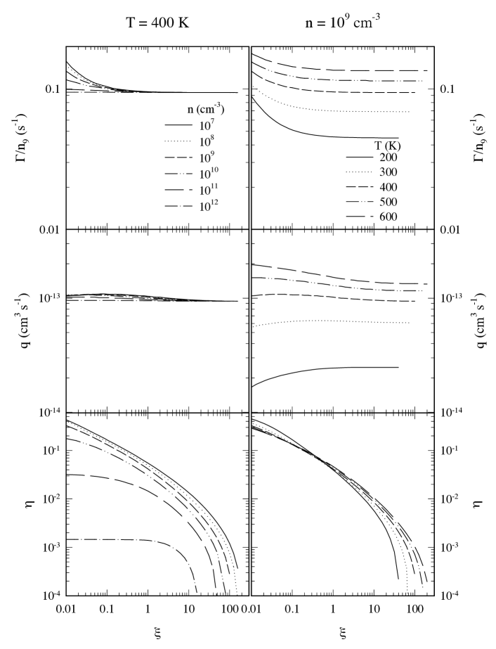
Figure 1: Modeling results for ${\rm H_{2}O}$ pumping at $T$ = 400 K and various densities (left panels) and at $n$ = $10^{9}$ cm^-3 and various temperatures (right panels). Plotted are the maser loss rate $\Gamma$, mean pump rate coefficient $q$ and inversion efficiency $\eta$ (Equation 2-6) as functions of the scaling parameter $\xi$ (Equation 2-4).

Figure 1 shows our results for the three pump parameters as functions of $\xi$ for a range of $n$ and $T$ relevant to observable masers. The scaling behavior of $\Gamma/n$, $q$ and $\eta$ is evident from the left column panels, which show their variation with $\xi$ at a fixed temperature. Even though the plots span five orders of magnitude in density, all three quantities are largely independent of $n$ whenever $\xi\,\raise 1.29167pt\hbox{$>$}\kern-7.5pt\lower 3.01385pt\hbox{$\sim$}\,0.1$; scaling breaks down only for $\eta$ when $n\,\raise 1.29167pt\hbox{$>$}\kern-7.5pt\lower 3.01385pt\hbox{$\sim$}\,\hbox{$10^{10}$}$ cm^-3. Moreover, both $\Gamma/n$ and $q$ are further independent of $\xi$ when $\xi\,\raise 1.29167pt\hbox{$>$}\kern-7.5pt\lower 3.01385pt\hbox{$\sim$}\,0.1$, indicating that all level populations are close to thermal equilibrium. The temperature variation of these pump parameters, shown in the right-column panels, is well described by the simple analytic approximations

$$\Gamma_{-1}\simeq 2.6n_{9}\,e^{-400/T},\qquad q_{-13}\simeq 3.2\,e^{-460/T},$$ (2-7)

where $\Gamma_{-1}=\Gamma/(\hbox{$10^{-1}$}\ \rm s^{-1})$ and $q_{-13}=q/(\hbox{$10^{-13}$}\ {\rm cm^{3}~{}s^{-1}})$. The accuracy of both expressions is within a few percent at all $T\,\raise 1.29167pt\hbox{$>$}\kern-7.5pt\lower 3.01385pt\hbox{$\sim$}\,300$ K and $\xi\,\raise 1.29167pt\hbox{$>$}\kern-7.5pt\lower 3.01385pt\hbox{$\sim$}\,0.1$; at $T$ = 200 K, the deviations reach only $\sim$ 25%.

As first noted by de Jong (1973), rotation levels on the “backbone” ladder (the lowest level for each $J$) carry the bulk of the ${\rm H_{2}O}$ population and establish a thermal equilibrium among themselves. Levels off the backbone, including the $J_{K-K+}=6_{16}$ and 5₂₃ maser levels, are populated predominantly by decays from higher backbone levels. This pattern leads to a number of inverted transitions, with the 22 GHz having the longest wavelength (1.35 cm) among them. Located 644 K above ground, the off-backbone 22 GHz maser system contains such a tiny fraction of the ${\rm H_{2}O}$ molecules ($\sim$1% even at the highest temperatures considered here) that it can be inverted with little impact on the overall thermal distribution of level populations. The inversion occurs because small contributions from radiative decays provide sufficient competition with the collisions to maintain $p_{2}>p_{1}$ over a wide range of parameters; we find that inversion is produced up to a density $n$ = 2$\times$$10^{12}$ cm^-3, although significant suppression of the maser line occurs for $n\,\raise 1.29167pt\hbox{$>$}\kern-7.5pt\lower 3.01385pt\hbox{$\sim$}\,10^{10}$ cm^-3. The bottom panels of Figure 1 show the inversion efficiency $\eta$. The right panel shows that $\eta$ is largely temperature independent for $T>200$ K, while the left panel displays the scaling property first noted in EHM: when expressed as a function of $\xi$, $\eta$ is independent of density as long as $n\,\raise 1.29167pt\hbox{$<$}\kern-7.5pt\lower 3.01385pt\hbox{$\sim$}\,\hbox{$10^{10}$}$ cm^-3. Indeed, $\eta$ is well described over the entire displayed range by the analytical approximation

$$\eta_{-2}\simeq{4.5\over\xi^{0.5}}\,c_{\eta}$$ (2-8)

where $\eta_{-2}=\eta/\hbox{$10^{-2}$}$ and where the correction factor

$$c_{\eta}=\frac{1}{1+0.01\,n_{9}^{1.15}\xi^{-0.5}}\hbox{$\times$}\frac{1}{1+0.015\,n_{9}^{0.2}\xi^{1.5}}$$ (2-9)

displays explicitly the deviations from scaling and the thermalizing, inversion-quenching effects of high densities and large optical depths. This approximation reproduces the numerical results to within $\sim$ 20% over the entire phase space volume displayed in Figure 1, except for its very edge at large $\xi$.

2.3 Maser Geometry

The quantities $\eta$, $q$ and $\Gamma$ fully determine the pumping scheme, enabling a complete solution of any maser model once its geometry is specified. The planar geometry of the slab is the key to strong maser action. It allows easy escape for the thermal photons through the slab thickness $d$, enabling inversion everywhere. Simultaneously, maser amplification in the plane can proceed along distance $ad$, where in principle the aspect ratio $a$ is arbitrarily large but in practice is limited either by the curvature of the shock or by the pathlength in the shock plane where velocity gradients shift the component in the plane by the thermal width (see §5). The resulting radiation is strongly beamed in the plane of the slab, and the strongest masers will be seen from edge-on orientations. Indeed, Marvel et al (2008) find that the outflows of the water maser associated with IRAS 4A/B in the star-forming region NGC 1333 are nearly in the plane of the sky, with inclination of only 2^∘ for IRAS 4A and about 13^∘ for IRAS 4B.

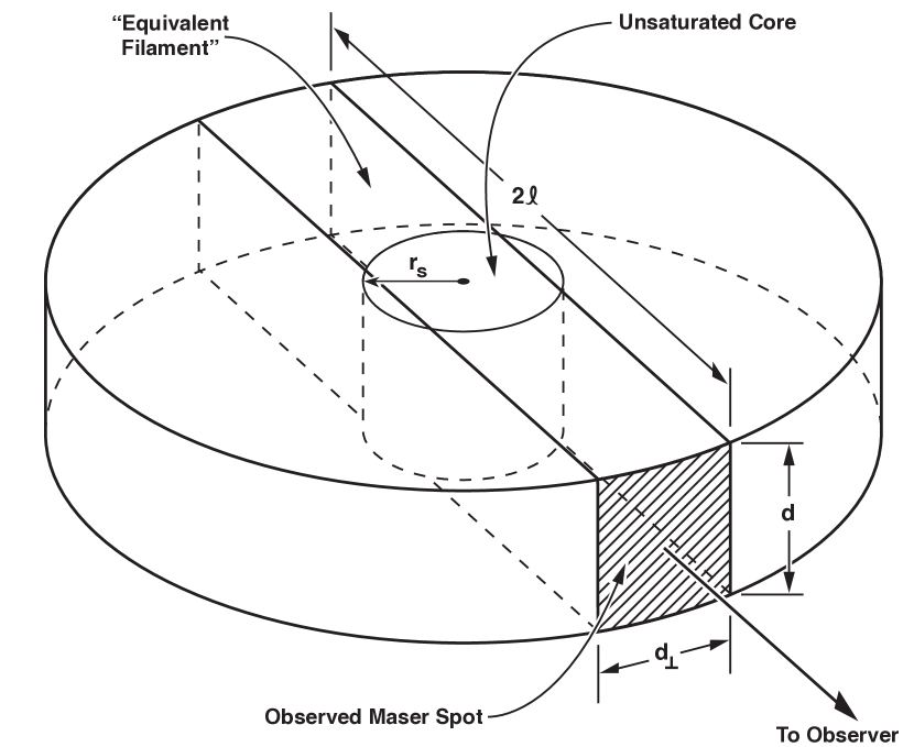
Figure 2: Illustration of the geometry of the shock maser model. The warm H₂O forms a slab of thickness $d$ behind the shock front, in the plane of the shock. A simple model for the region of velocity coherence is that of a planar disk of diameter $2\ell$. The maser aspect ratio is defined as $a\equiv 2\ell/d$. However, the results of this paper apply to any velocity coherent region in a slab that has its longest dimension $2\ell>d$. An unsaturated central region of radius $r_{s}$ forms. The masing photons are beamed out in rays in the disk plane passing through the unsaturated core. The observer sees a maser spot size $d\times\hbox{$d_{\perp}$}$, where $d_{\perp}$ is defined in Equation (B6). EHM92 show that $d_{\perp}/r_{s}=(\pi/(\kappa_{0}r_{s}))^{1/2}$ so that $d_{\perp}/r_{s}$ ranges from $\sim 0.5$ when the maser is just saturated to $\sim 1$ when the maser approaches core saturation (see Appendix B).

The general solution of planar masers is presented in EHM92. Its essentials are reproduced in Appendix B, together with a glossary of key dimensions in Table 1. The aspect ratio $a$ is the most important geometrical property of such masers; for a circular disk with radius $\ell$ and thickness $d$ (Figure 2) it is

$$a={2\ell\over d}.$$ (2-10)

The shape of the masing material in the plane is largely irrelevant once the maser saturates. For a circular ${\rm H_{2}O}$ maser disk, the aspect ratio required to bring about maser saturation is

$$\hbox{$a_{\rm sat}$}\simeq 3.6{n_{9}\over\xi^{1/2}c_{\eta}}\,e^{60/T}\left[1-{21\over T}+0.12\ln\,{n_{9}\over\xi^{1/2}}\right],$$ (2-11)

obtained by inserting into the general expression for this geometry, reproduced in Equation (B3), the results of the ${\rm H_{2}O}$ pumping scheme (Equations A8 and A12). For comparison, the analogous expression for a cylindrical maser with diameter $d$ is listed in Equation (B4) in Appendix B. The two saturation aspect ratios are nearly identical in ${\rm H_{2}O}$ masers, the differences mostly involving small logarithmic corrections. Since the saturation condition is the same for the two extremes of planar geometrical shape, this ensures that maser saturation is controlled solely by the length of the velocity coherent region.

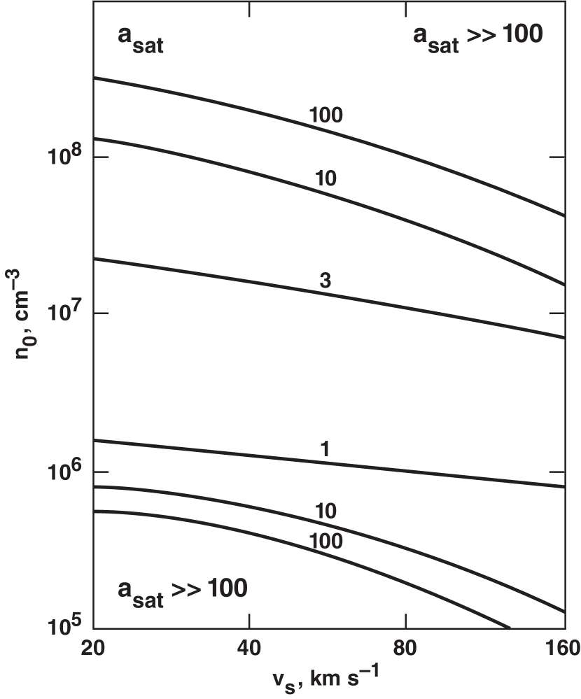
Figure 11: The saturation aspect ratio $a_{\rm sat}$ is plotted as a function of $n_{0}$ and $v_{s}$. High aspect ratios ($a\,\raise 1.29167pt\hbox{$>$}\kern-7.5pt\lower 3.01385pt\hbox{$\sim$}\,30-100$), or high coherence lengths relative to $d$, are not often achieved in interstellar J shocks.

With $\kappa_{0}$ the unsaturated absorption coefficient, the quantity $\hbox{$a_{\rm sat}$}\,\hbox{$\kappa_{0}$}d$ is the maser optical depth along the disk diameter at saturation (cf Equation A12); it is a measure of the amplification required along the maser longest path in order to bring saturation. As is evident from Equation (B3), this quantity has similar values for all pumping conditions, varying only logarithmically with the pumping parameters; some general arguments show that the intrinsic properties of the ${\rm H_{2}O}$ molecule imply $\hbox{$a_{\rm sat}$}\,\hbox{$\kappa_{0}$}d\sim$ 15 (E92; see also Eq. B3). Strong masers can be expected when saturation is reached at realistic elongations, i.e., moderate aspect ratios $a_{\rm sat}$ ( $<$$\sim$  10). As we show below (see §4, in particular Figure 11), J shocks produce $a_{\rm sat}$  $<$$\sim$  5 over a large volume of parameter space, ensuring strong maser action for a wide range of conditions. The near constancy of $a_{\rm sat}$ over such a large parameter region implies that $\hbox{$\kappa_{0}$}d$ (roughly proportional to 1/$a_{\rm sat}$; see Eq. B3) too has only moderate variation there.

As noted in EHM92, saturated masers can be distinguished by two types of beaming. For amplification-bounded masers, whose prototype is the spherical maser, the beaming angle depends on the amplification. These masers are characterized by observed sizes significantly smaller than their projected physical size. Furthermore, the observed size increases with frequency shift from line center (Elitzur 1990). Such increases have been reported in a recent study of ${\rm H_{2}O}$ masers around evolved stars (Richards et al 2011). For matter-bounded masers, whose prototype is the filamentary maser, the beaming angle depends only on the geometry of the maser. They are characterized by observed sizes that are equal to their projected physical size and constant across the line profile. In principle, saturated planar masers produced by shocks can display both types of behavior. For a shock moving across the line of sight (shock velocity vector $\mathbf{v}_{s}$ in the plane of the sky), denote by $\|$ the direction parallel to $\mathbf{v}_{s}$ and by $\perp$ the direction orthogonal to both $\mathbf{v}_{s}$ and the line of sight. The dimension of the masing medium along the $\|$-direction is the slab thickness, $d$, and the dimension along the line of sight is $2\ell=ad$. Whereas $d$ is determined by the structure of the shock, the dimensions of the masing medium in the two directions in the slab plane are controlled by other factors, such as velocity coherence and shock curvature. We term planar masers that are matter bounded in the $\|$-direction “thin,” and those that are amplification bounded in that direction “thick.”

Appendix B presents a detailed description of both thin and thick disk masers, and Table 1 provides a glossary of maser dimensions relevant for the two cases. As we shall see below, most interstellar shocks are “thin,” with the maser structure as depicted in Figure 2. Let $d_{\|}$ denote the observed size of the maser parallel to the shock velocity and $d_{\perp}$ the observed size in the plane of the sky normal to the shock velocity. A thin maser is matter bounded in the $\|$-direction and amplification bounded in the $\perp$-direction, therefore $\hbox{$d_{\|}$}=d$ but $d_{\perp}$ is smaller than $ad$, the physical size in the $\perp$-direction. Inserting the results of the ${\rm H_{2}O}$ pumping scheme (Eq. A12) into Equation (B6) and utilizing Equation (2-11), the ratio $d/d_{\perp}$ is given by

$${d\over\hbox{$d_{\perp}$}}\simeq{3.3\over\hbox{$a_{\rm sat}$}}\hbox{$\times$}\frac{\displaystyle 1-{21\over T}+0.12\ln\,{n_{9}\over\xi^{1/2}}}{\displaystyle\left[1-{14\over T}+0.26\ln\,{n_{9}\over(\xi c_{\eta})^{1/2}}-0.13\ln a\right]^{1/2}}.$$ (2-12)

The maser will appear elongated either in the plane of the shock or along the shock propagation, depending on the value of $a_{\rm sat}$ that the pumping scheme generates.

2.4 Maser Brightness and Flux

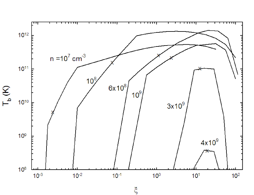
Figure 3: Brightness temperatures of disk masers with $a=10$ as functions of $\xi$ at $T=400$ K and different densities, as marked. On each curve, an X marks the value of $\xi$ generated by a J shock that produces the corresponding post-shock density for $v_{A\perp,5}=\hbox{$\Delta v_{D5}$}=1$ (see text for details).

We now discuss the predictions of the ${\rm H_{2}O}$ pumping scheme for observable radiative quantities. These results are applicable only for the emission from resolved individual maser spots. The brightness temperature at line center is given by Equations (B14) and (B20), respectively, for the unsaturated and saturated regimes. While the pump properties can be specified in terms of density-independent scaling quantities, the onset of saturation does involve the density (Equation 2-11). Figure 3 shows the variation of brightness temperature with $\xi$ for a wide range of densities for disk masers with $a=10$, chosen for illustration; the behavior for other aspect ratios can be deduced from the explicit expressions for $T_{b}$ shown below. Each curve shows a steep exponential rise at the low-$\xi$ end, corresponding to unsaturated maser growth. The break in the slope marks the onset of saturation, and the behavior of $T_{b}$ at higher values of $\xi$ is controlled by the variation of the maser pump properties. Saturation is reached for all the displayed densities except for $n=4\times\hbox{$10^{9}$}\,\hbox{cm${}^{-3}$}$, which falls just short of saturation—in that case $a_{\rm sat}$ = 13 around the peak of the $T_{b}$ curve. Therefore, $n\simeq 3\times\hbox{$10^{9}$}\,\hbox{cm${}^{-3}$}$ is the highest density that produces saturated disk masers with $a=10$ at $T$ = 400 K. The curves for $n=\hbox{$10^{7}$}$ and $10^{8}$ cm^-3 show an additional break at $\xi$ = 0.01 and 0.3, respectively. This break marks the transition to a thick disk regime, a transition that occurs only at lower densities (see Equation B8). Masers with $n\geq 6\times\hbox{$10^{8}$}\,\hbox{cm${}^{-3}$}$ are in the thin-disk domain for all values of $\xi$.

On each curve in the figure, an X marks the value of $\xi$ generated by a J shock with $v_{A\perp}=1$ km s^-1 and $\Delta v_{D}=1$ km s^-1 that produces a maser density corresponding to that curve, as described below (see §3). This shows that J shocks with $a=10$ produce saturated thin-disk masers in the entire range $\hbox{$10^{7}$}\,\hbox{cm${}^{-3}$}\ \leq n\leq 3\times\hbox{$10^{9}$}\,\hbox{cm${}^{-3}$}$. For thin-disk masers with $a>a_{\rm sat}$, the brightness temperature at line center can be written as

$$T_{b}\simeq 4.7\hbox{$\times$}\hbox{$10^{11}$}\,\xi^{1/2}c_{\eta}(d/\hbox{$d_{\perp}$})e^{-460/T}a_{1}^{3},$$ (2-13)

where $a_{1}=a/10$ (see Equation B22). This result amplifies our earlier findings (EHM, EHM92): Apart from the gas temperature, the brightness temperature of J-shock produced masers is determined almost exclusively by $\xi$ and the maser aspect ratio $a$. Further discussion of this effect appears in §4.1. The relevant quantity for maser detectability from a distance $D_{\rm kpc}$ in kpc is its observed monochromatic flux. From Equation (B19), the observed flux at line center is

$$F_{\nu_{0}}\simeq 74\,\xi^{1/2}c_{\eta}e^{-460/T}{d_{13}^{2}\over D_{\rm kpc}^{2}}a_{1}^{3}\quad\rm Jy.$$ (2-14)

Measured flux is frequently expressed in terms of the equivalent isotropic luminosity $L_{\rm iso}=4\pi D^{2}F$, where $F$ is the flux integrated over the spectral range of the maser feature. Then

$$L_{\rm iso}=4\pi D^{2}F_{\nu 0}\cdot\frac{\pi^{1/2}\hbox{$\Delta v_{D}$}}{\lambda}\simeq 3\hbox{$\times$}\hbox{$10^{-6}$}\xi^{1/2}c_{\eta}e^{-460/T}\hbox{$\Delta v_{D5}$}d_{13}^{2}a_{1}^{3}\quad\hbox{$L_{\odot}$}.$$ (2-15)

Because of the beaming, the actual luminosity of a planar maser is only $L_{m}=L_{\rm iso}/2a$ (EHM92).

3 J-SHOCK STRUCTURE IN VERY DENSE GAS

3.1 Review of J-Shock Structure and Analytic Results

A number of authors, including Hollenbach & McKee (1979, 1989; hereafter HM79, HM89), Neufeld & Dalgarno (1989), Neufeld & Hollenbach (1994), Smith & Rosen (2003), Guillet, Jones, & Pineau Des Forêts (2009), and Flower & Pineau Des Forêts (2010), have discussed J-shock structure in dense molecular gas. EHM discussed the particular structure found in the very dense J shocks that may give rise to 22 GHz water masers. In fast J shocks, the molecules are first completely dissociated by the extremely high postshock temperatures ($\sim 10^{5}$ K) immediately behind the shock front. In this very hot region, dust may be partially or totally destroyed by thermal sublimation, sputtering, and grain-grain collisions. Further downstream, where the material cools down, H₂ molecules reform on the surviving dust grains and are ejected to the gas phase with sizable internal energies, which provides a source of heating for the gas if the postshock densities are sufficiently high ($\,\raise 1.29167pt\hbox{$>$}\kern-7.5pt\lower 3.01385pt\hbox{$\sim$}\,10^{6}$ cm^-3) to convert this internal energy into heat. In other words, the rovibrationally excited H₂ molecule needs to be collisionally de-excited, rather than suffering radiative decay, for the energy to be converted to heat. This heating produces an “H₂ re-formation plateau,” a nearly isothermal column of gas at a temperature $T_{p}\sim 300-400$ K. The plateau gas is warm enough to drive all oxygen not locked in CO to form H₂O and to collisionally populate the 22 GHz maser levels, which lie $644$ K above ground. The dust temperature in the masing region is typically 50-100 K. The hydrogen column density, $N_{p}$, of the heated plateau region can be as large as $\sim 10^{22-23}$ cm^-2, and the H₂O column as high as 3$\times 10^{19}$ cm^-2. The H₂ re-formation plateau is an ideal site for relatively low-lying H₂O masers like the 22 GHz masers; the temperature $T_{p}$ may be too low to significantly excite higher excitation H₂O maser levels, and C shocks have been proposed as sites of those masers (Melnick et al 1993, Kaufman & Neufeld 1996).

In both C and J shocks, the component of the magnetic field normal to the shock velocity, $B_{0\perp}$, serves to limit the compression of the postshock gas. This component of the magnetic field is related to the corresponding preshock Alfven speed $v_{A\perp}$ by

$$B_{0\perp}=1.7v_{A\perp,5}n_{0,7}^{1/2}\ {\rm mG},$$ (3-1)

where $v_{A\perp,5}=v_{A\perp}/(1$ km s^-1) and where $n_{0,7}=n_{0}/(10^{7}$ cm^-3) is the density of hydrogen nuclei in the preshock gas [i.e., $n_{0}=n_{0}$(H)$+2n_{0}$(H${}_{2})$]. If the shock velocity and the orientation of the magnetic field are uncorrelated, the median value of $B_{0\perp}$ equals $(\surd 3/2)B_{0}$, so the distinction between $B_{0}$ and $B_{0\perp}$ is not numerically important. Nonetheless, we shall retain this distinction here since future observations might be able to determine the relative orientations of the shock velocity and the upstream magnetic field. Typical preshock magnetic fields in molecular clouds of widely varying density are characterized by preshock Alfven speeds $v_{A}\sim 1-2$ km s^-1 (Heiles et al 1993). Fields at high densities have recently been measured by Falgarone et al (2008) who observed the Zeeman effect in CN. For the 8 measurements with positive detections, the median value of $v_{A5}$ is 1. Including the 6 measurements with no detections, but using the quoted error as the value, we find a median of 0.6. The dispersion is large, however: a factor 6. Correcting for inclination, we estimate $v_{A5}\simeq 1\pm 0.8$ dex. This is quite crude, however, since our treatment of the upper limits is very approximate and since the Zeeman technique averages over fluctuations in the line-of-sight field. As noted above, typically $v_{A\perp}\simeq v_{A}$ if the orientations of of the shock velocity and the magnetic field are uncorrelated, so we shall adopt $v_{A\perp,5}=1$ as a fiducial value.

The density $n_{p}$ in the masing (“plateau”) region of a J shock is usually limited by the value of $B_{0\perp}$ (HM79), and can be written as $n_{p}=\surd 2n_{0}v_{s}/v_{A\perp}$. In terms of the flux of H nuclei through the shock, $j\equiv n_{0}v_{s}$, we have

$$n_{p9}\equiv\frac{n_{p}}{10^{9}\ {\rm cm^{-3}}}=1.4\left(\frac{j_{14}}{v_{A\perp,5}}\right),$$ (3-2)

where

$$j_{14}\equiv n_{0,7}v_{s7},$$ (3-3)

$v_{s7}\equiv v_{s}/(100$ km s^-1) is the shock speed in units of 10⁷ cm s^-1, and $j_{14}=j/(10^{14}$ cm^-2 s^-1). We shall find that many of masing parameters mainly depend on $j$. The magnetic field in the masing region of a J shock balances the ram pressure of the shock and is therefore independent of the preshock field,

$$B_{p}\simeq 0.24n_{0,7}^{1/2}v_{s7}\ \mbox{G}=0.24j_{14}^{1/2}v_{s7}^{1/2}\ \mbox{G}=0.24j_{14}n_{0,7}^{-1/2}\ \mbox{G}.$$ (3-4)

The analytic formulae for the density $n_{p}$ and the magnetic field $B_{p}$ in the maser region apply when the magnetic pressure dominates there, or when $v_{A\perp,5}\,\raise 1.29167pt\hbox{$>$}\kern-7.5pt\lower 3.01385pt\hbox{$\sim$}\,2\times 10^{-2}v_{s7}^{-1}$, assuming the plateau temperature is 300-400 K (HM79, EHM). Since $v_{A\perp,5}$ is usually $\,\raise 1.29167pt\hbox{$>$}\kern-7.5pt\lower 3.01385pt\hbox{$\sim$}\,0.2$, this condition is readily met.

Table 2 summarizes analytic solutions and approximations previously obtained in HM79, HM89, and EHM, or, in the case of $T_{b}$ and $L_{\rm iso}$, taken from Section 2 . We define $T_{b,11}\equiv T_{b}/10^{11}$ K and $L_{\rm iso,-6}\equiv L_{\rm iso}/(10^{-6}\;L_{\odot})$. The factor $\gamma=10^{-17}\gamma_{-17}$ cm³ s^-1 is the average rate coefficient for H₂ formation on grains in the temperature plateau region. In our numerical shock computations we use the formulation for $\gamma$ from HM79. Note that because of the gas and dust temperature sensitivity of $\gamma$ and because partial destruction of dust near the shock front reduces the area of grains and therefore $\gamma$, there is a “hidden” additional dependence on $n_{0}$ and $v_{s}$, or on $d$ and $v_{A\perp}$, when $\gamma$ appears in Table 2. The same holds true for $x_{-4}({\rm H_{2}O})$. However, Table 2 is general to any formulation for $\gamma$ and for any postshock H₂O abundance, in contrast to the tables presented later in §4.2 that are specific to our particular formulation of $\gamma$ and to our shock chemistry, which derives $x_{-4}({\rm H_{2}O})$ at each point in the postshock gas. The column density in the masing region (or the H₂ re-formation plateau region), $N_{p}$, is analytically determined by finding the timescale $t_{\rm H_{2}}$ for H₂ formation in the plateau and then taking $N_{p}=n_{0}v_{s}t_{\rm H_{2}}$ (EHM). The timescale $t_{\rm H_{2}}$ is given by

$$t_{\rm H_{2}}={1\over{n\gamma}}$$ (3-5)

leading then to

$$N_{p}=7\times 10^{21}\left({v_{A\perp,5}\over\gamma_{-17}}\right)\ {\rm cm^{-2}}$$ (3-6)

The thickness $d$ of the postshock masing region (the spot size parallel to the shock velocity) is given by

$$d=\frac{N_{p}}{n_{p}}=5.0\times 10^{12}\;\frac{v_{A\perp,5}^{2}}{\gamma_{-17}j_{14}}$$ (3-7)

The formulae for $N_{p}$ and $d$ are quite accurate when applied to the numerical results, but require a knowledge of $\gamma_{-17}$. The value of $\gamma_{-17}$ is of order 0.1-3.0 (HM79) for the gas and dust temperatures typical of the masing plateau. Note that the column density in the plateau is independent of the preshock density and shock velocity or of $j$, for fixed $\gamma$. The analytic formulae for $\xi$, $T_{b}$, and $L_{\rm iso}$ in the masing region come from Equations (2-4), (2-15), and (2-17), respectively. The expressions for $n_{p}$, $T_{p}$, $d$, $\xi$, $T_{b}$ and $L_{\rm iso}$ in Table 2 depend only on $j$ and not separately on $n_{0}$ and $v_{s}$. The parameter $B_{p}$ is the sole parameter dependent on the additional parameter $v_{s}$, but only as the square root.

Table 2 tabulates quantities in terms of the preshock variables $j$ and $v_{A\perp}$ in column 1 and in terms of the observable quantities $d$, $d/d_{\perp}$ (the ”shape” of the maser spot) and $v_{A\perp}$ in column 2. Essentially, we have eliminated $j=n_{0}v_{s}$ from column 1 in favor of $d$ in column 2. Column 2 is added to aid observers in estimating the shock parameters. However, it must be noted that the average values of $\gamma_{-17}$, $x_{-4}({\rm H_{2}O})$, and $\Delta v_{D5}$ in the masing plateau appear in these equations. As we will see in the subsections below, these all have values near unity for most cases, enabling an estimate to be made of the shock parameters. The numerical results presented in this paper can be understood, interpolated and extrapolated by applying these formulae.

3.2 Physical Processes in the J-shock Model

HM79, HM89 and Neufeld & Hollenbach (1994) describe in detail the physical processes included in the 1D steady state shock code we have used in this paper. The fundamental input parameters to this code are the preshock hydrogen nucleus density $n_{0}$, the shock velocity $v_{s}$, the Alfven speed $v_{A\perp}$ in the preshock gas, the velocity dispersion $\Delta v_{D}$ in the line-emitting gas, and the gas phase abundances of the elements. In our standard runs we take $v_{A\perp}=1$ km s^-1, $\Delta v_{D}=1$ km s^-1, and gas phase abundances listed in HM89 (the main number abundances relative to hydrogen nuclei that are relevant here are those for carbon, 2.3$\times 10^{-4}$, and oxygen, 5.4$\times 10^{-4}$).

The code uses the Rankine-Hugoniot jump conditions to set the physical parameters immediately behind the shock front, and the various continuity equations to numerically solve for the temperature, density and chemical structure in the cooling postshock gas. The chemistry includes 35 species and about 300 reactions. For the fast ($v_{s}\,\raise 1.29167pt\hbox{$>$}\kern-7.5pt\lower 3.01385pt\hbox{$\sim$}\,20$ km s^-1), dense ($n_{0}\,\raise 1.29167pt\hbox{$>$}\kern-7.5pt\lower 3.01385pt\hbox{$\sim$}\,10^{5}$ cm^-3) shocks considered in this paper, important chemical processes include collisional dissociation and ionization, photodissociation and photoionization by the UV photons produced in the (upstream) hot postshock gas, neutral-neutral reactions with activation barriers, and the re-formation of H₂ molecules on warm ($T_{\rm gr}\simeq 50-150$ K) dust grains. All but the last are either well determined experimentally or well understood theoretically.

We discuss here the formation rate coefficient of H₂ on warm dust grains in some detail, as this process is critical to forming the high temperature plateau where the H₂O maser is produced. We use the theoretical model of HM79 for the formation of H₂ on warm grains. In this formulation the formation rate coefficient $\gamma$ is a function of both the gas temperature $T$ and the dust temperature $T_{\rm gr}$. At relatively low $T$ ($\,\raise 1.29167pt\hbox{$<$}\kern-7.5pt\lower 3.01385pt\hbox{$\sim$}\,100$ K) and $T_{\rm gr}$ ($\,\raise 1.29167pt\hbox{$<$}\kern-7.5pt\lower 3.01385pt\hbox{$\sim$}\,30$ K), the rate coefficient has been inferred observationally in diffuse clouds and molecular cloud surfaces to be $3\times 10^{-17}$ cm³ s^-1. At the somewhat higher gas temperatures $T\sim 400$ K in the plateau, the coefficient drops by about a factor of $\sim$ 2 due to the decreased sticking probability of incoming H atoms (e.g., HM79, Cuppen et al 2010). However, a more important effect in the plateau is caused by the increased $T_{\rm gr}\sim 100$ K, which causes $\gamma$ to drop even more because of the evaporation of H atoms from grain surfaces prior to H₂ formation. The exact amount of this drop cannot be well determined for realistic interstellar dust. However, HM79, Cuppen et al (2010), and Cazaux et al (2011) have used theoretical modeling to try to estimate the effect. All three of these studies are in quite good agreement, given the inherent uncertainties. Including both the sticking probability and the probability of H₂ formation on the grain surface, and normalizing to obtain the above standard rate at low $T$ and $T_{\ gr}$, Cuppen et al get a H₂ rate coefficient for 400 K gas and 100 K dust of $2.2\times 10^{-18}$ cm³ s^-1, whereas HM79 find $3.8\times 10^{-18}$ cm³ s^-1. In addition, Cazaux et al find a rate coefficient for 400 K gas and 125 K dust of $1.5\times 10^{-18}$ cm³ s^-1, whereas HM79 find $1.4\times 10^{-18}$ cm³ s^-1. Therefore, the HM79 formation rate coefficient agrees well with the more recently obtained values in the region of parameter space ($T\sim 400$ K, $T_{gr}\sim 100$ K) where the H₂ re-forms in the postshock gas, and where the H₂O maser is produced. This agreement is far better than the uncertainties in these models, and therefore there could be fairly large differences between these values and the values for real shocked grains at high dust temperatures. Because of these uncertainties, we consider the sensitivity of our results to the H₂ formation rate coefficient in the next subsection.

Our model also includes the partial destruction of dust grains in the shock, which reduces the grain surface area per H nucleus, and which therefore also reduces the rate coefficient for H₂ formation on grains. Our J-shock maser model relies on at least some grains surviving the shock, since the H₂ re-formation plateau is caused by H₂ re-formation on grain surfaces. However, shocks with $v_{s}\,\raise 1.29167pt\hbox{$>$}\kern-7.5pt\lower 3.01385pt\hbox{$\sim$}\,200$ km s^-1 will completely destroy dust grains by sputtering and grain-grain collisions (Jones et al 1996). We therefore only consider shocks with $v_{s}<200$ km s^-1. In addition, shocks with $n_{0,7}v_{s7}^{3}\,\raise 1.29167pt\hbox{$>$}\kern-7.5pt\lower 3.01385pt\hbox{$\sim$}\,100$ will sublimate all grains with sublimation temperatures $T_{\rm sub}\,\raise 1.29167pt\hbox{$<$}\kern-7.5pt\lower 3.01385pt\hbox{$\sim$}\,1500$ K, which is the maximum sublimation temperature of a likely interstellar grain material. Therefore, no dust exists above this constraint as well. For $n_{0}$ and $v_{s}$ values that are low enough to provide at least some dust survival, we adopt the grain composition mixture of Pollack et al (1994), and allow for the sublimation of the less refractory material at lower values of $n_{0,7}v_{s7}^{3}$ as each sublimation temperature is exceeded.

In summary, the conditions $n_{0,7}v_{s7}^{3}\,\raise 1.29167pt\hbox{$<$}\kern-7.5pt\lower 3.01385pt\hbox{$\sim$}\,100$ and $v_{s7}\,\raise 1.29167pt\hbox{$<$}\kern-7.5pt\lower 3.01385pt\hbox{$\sim$}\,2$ provide upper limits for J-shock masers produced by the H₂ re-formation plateau. We find below, however, somewhat more stringent conditions on preshock density occur due to the quenching of the H₂O maser by high postshock densities and H₂O line optical depths. An example of this is shown in Figure 3, which shows the quenching that occurs in the case of slabs with $a=10$ and $v_{A\perp,5}=\hbox{$\Delta v_{D5}$}=1$; the maser is quenched for $n_{p}\geq 4\times 10^{9}$ cm^-3 since then $\hbox{$a_{\rm sat}$}>a$. The upper limit on the preshock density for effective maser emission in this particular case is therefore $n_{0}\,\raise 1.29167pt\hbox{$<$}\kern-7.5pt\lower 3.01385pt\hbox{$\sim$}\,3\times 10^{7}\left(v_{A\perp,5}/v_{s7}\right)~{}{\rm cm^{-3}}$ from Equation (3-2).

The cooling of the postshock gas is treated with the escape probability formalism (including the effects of dust absorption), since a number of important cooling transitions become optically thick in the lines. For this study, we focus mainly on the postshock temperature region bounded by 3000 K $>T>$ 50 K, where molecular formation occurs and H₂O masers may be produced. In the masing region, the gas cooling is dominated by optically thick rotational transitions of H₂O and by gas collisions with the cooler dust grains. The gas heating in the masing region is dominated by the re-formation of H₂. There are two main contributions to this heating process. The newly formed molecules can be ejected from the grain surfaces with kinetic energies greater than $kT$, thereby heating the gas. In addition, a newly formed and ejected molecule may carry with it rovibrational energy that can be transferred to heat by collisional de-excitation in the gas. These processes are not well determined. We adopt the theoretical formulation of HM79, in which the newly formed molecule is ejected with 0.2 eV of kinetic energy and 4.2 eV of rovibrational energy and use the de-excitation rate coefficients for H and H₂ collisions quoted in HM79. However, Tielens and Allamandola (1987) speculate that the H₂ molecule may lose a significant portion of its formation energy (the rovibrational energy) to the grain, before leaving the grain surface. Since the formation heating is proportional to the H₂ formation rate times the energy delivered per H₂ to the gas, we test the sensitivity of our results to the energy partition when we test the sensitivity of the plateau temperature to the uncertain formation rate coefficient.

3.3 Numerical Results for J-shock Structure

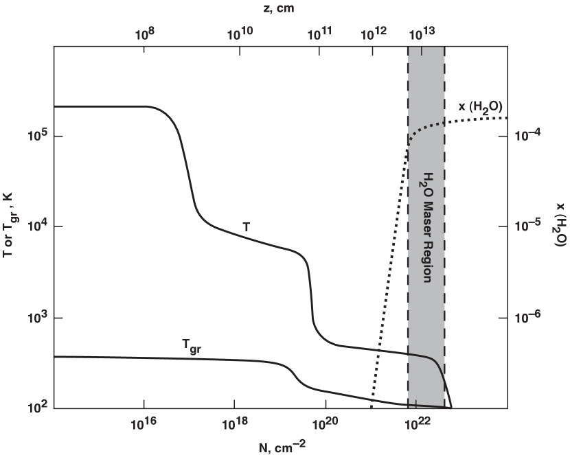
Figure 4: Shock structure for the standard run with preshock density $n_{0}=10^{7}$ cm^-3 ($n_{0,7}=1$), shock velocity $v_{s}=100$ km s^-1 ($v_{s7}=1$), and preshock magnetic field given by the Alfven speed $v_{A\perp}=1$ km s^-1 ($v_{A\perp,5}=1$). The $x$ axis (bottom) is the column density $N$ of hydrogen nuclei downstream from the shock front; the $x$ axis (top) is the corresponding distance $z$. The $y$ axis (left) is the temperature ($T$, $T_{\rm gr}$) of the (gas, dust grains); the $y$ axis (right) is the abundnace of H₂O. Key features include $T_{\rm gr}\ll T$ and the gas temperature plateau $T\simeq T_{p}\simeq 350$ K from $N\simeq 10^{20.5}-10^{22.5}$ cm^-2 caused by the heating due to H₂ re-formation. This plateau region includes a large column of warm H₂O molecules that are collisionally-excited to mase at 22 GHz.

Figure 4 presents the shock profile for our standard model: $n_{0}=10^{7}$ cm^-3, $v_{s}=100$ km s^-1, $v_{A\perp}=1$ km s^-1, and $\Delta v_{D}=1$ km s^-1. The column density of hydrogen nuclei, $N$, and the position, $z$, are measured from the shock front. The ultraviolet radiation from the shock has processed the preshock gas before it enters the shock front. As a result, the molecular preshock gas is photodissociated and partially photoionized prior to being shocked. Using the results of HM89, we take the initial abundances at the shock front for the standard case to be $x(H^{+})=0.47$, $x(H)=0.36$, $x(H_{2})=0.087$; the trace species are largely atomic and singly ionized as well. For slower shocks, the precursor field is less important and the shock front abundances are initially largely molecular. The gas then collisionally dissociates and partially ionizes in the hot postshock gas just downstream of the shock front. Figure 4 shows that the 100 km s^-1 shock heats the plasma to about $2\times 10^{5}$ K, and the gas cools by collisional ionization and by UV and optical emission to 10⁴ K in a column $N\simeq 4\times 10^{17}$ cm^-2. The Lyman continuum photons from the $\sim 10^{5}$ K gas maintain a Strömgren region at $T\sim 10,000$ K to a column $N\simeq 10^{19.5}$ cm^-2. Once the Lyman continuum photons are absorbed, the electrons and protons recombine and the gas cools until the heating due to H₂ re-formation maintains the temperature at $T_{p}\simeq 300-400$ K. This is the “H₂ re-formation plateau”. Note that the size scale of this plateau, shown at the top of the figure, is $d\sim 10^{13}$ cm for $v_{A\perp}=1$ km^-1 and for our assumed formulation for $\gamma_{-17}$. After the molecular hydrogen has nearly completely reformed, at a column of about $2\times 10^{22}$ cm^-2, the heating rate drops and the gas temperature drops to $\,\raise 1.29167pt\hbox{$<$}\kern-7.5pt\lower 3.01385pt\hbox{$\sim$}\,100$ K.

The H₂O number abundance relative to hydrogen nuclei, $x$(H₂O), is also plotted in Figure 4. The abundance is negligible for $N\,\raise 1.29167pt\hbox{$<$}\kern-7.5pt\lower 3.01385pt\hbox{$\sim$}\,10^{21}$ cm^-2, but the H₂O abundance rapidly climbs once the H₂ abundance rises in the re-formation plateau. CO re-forms even more rapidly; typically all the gas phase carbon is incorporated into CO once $x$(H₂)$\,\raise 1.29167pt\hbox{$>$}\kern-7.5pt\lower 3.01385pt\hbox{$\sim$}\,10^{-3}$. Therefore, the abundance of H₂O is limited to the abundance of oxygen that remains once an oxygen atom has combined with every gas phase carbon atom. We have taken for elemental gas phase abundances $x_{\rm O}$=$5.4\times 10^{-4}$ and $x_{\rm C}$=$2.3\times 10^{-4}$; thus, $x_{\rm max}$(H₂O)$\simeq 3\times 10^{-4}$. Typically, $x$(H₂O)$\simeq x_{\rm max}$(H₂O) once $x$(H₂) $\,\raise 1.29167pt\hbox{$>$}\kern-7.5pt\lower 3.01385pt\hbox{$\sim$}\,0.25$. However, the reactions that lead to H₂O have large activation energies ($\Delta E/k\sim 4000$ K) and proceed slowly in the plateau region. In many cases the timescales spent in the plateau are insufficient to reach chemical equilibrium; as a result, the H₂O abundance varies somewhat with $T_{p}$ and $N_{p}$ and consequently with $n_{0}$ and $v_{s}$, as shall be demonstrated below.

We have also plotted the grain temperature, $T_{\rm gr}$, in Figure 4 to emphasize the fact that the grain temperature is significantly below the gas temperature in the postshock gas if $n_{0,7}v_{s7}^{3}\,\raise 1.29167pt\hbox{$<$}\kern-7.5pt\lower 3.01385pt\hbox{$\sim$}\,100$ (HM79). The grains are only weakly coupled to the gas through gas collisions and through the line radiation from the gas. At the same time, radiative grain cooling is very efficient; the result is that the grains are considerably cooler than the gas. Because the dust is optically thin in the H₂O rotational transitions and the lines themselves have finite opacity, the effective temperature of the radiation field is cooler than the gas kinetic temperature. Consequently, collisions with H atoms and H₂ molecules excite the H₂O and the escaping IR photons from H₂O rotational transitions create non-LTE populations and the population inversion of the maser levels. Absorption by dust competes with escape of the IR photons when the dust optical depth reaches unity for the IR photons; for ${\rm H_{2}O}$ IR photons with typical wavelengths of 50 $\mu$m, this occurs at a column density $N_{p}\simeq 3\times 10^{23}$ cm^-2 if we account for some reduction in dust abundance in the shock (HM79). Using the expression for $N_{p}$ in Table 2, we estimate that dust absorption is not important for

$${\gamma_{-17}\over v_{A\perp,5}}\,\raise 1.29167pt\hbox{$>$}\kern-7.5pt\lower 3.01385pt\hbox{$\sim$}\,0.02,$$ (3-8)

which is generally the case. If dust absorption is important, and the dust is cooler than the gas, the presence of dust enhances the effective escape probability of the H₂O IR photons (Collison & Watson 1995).

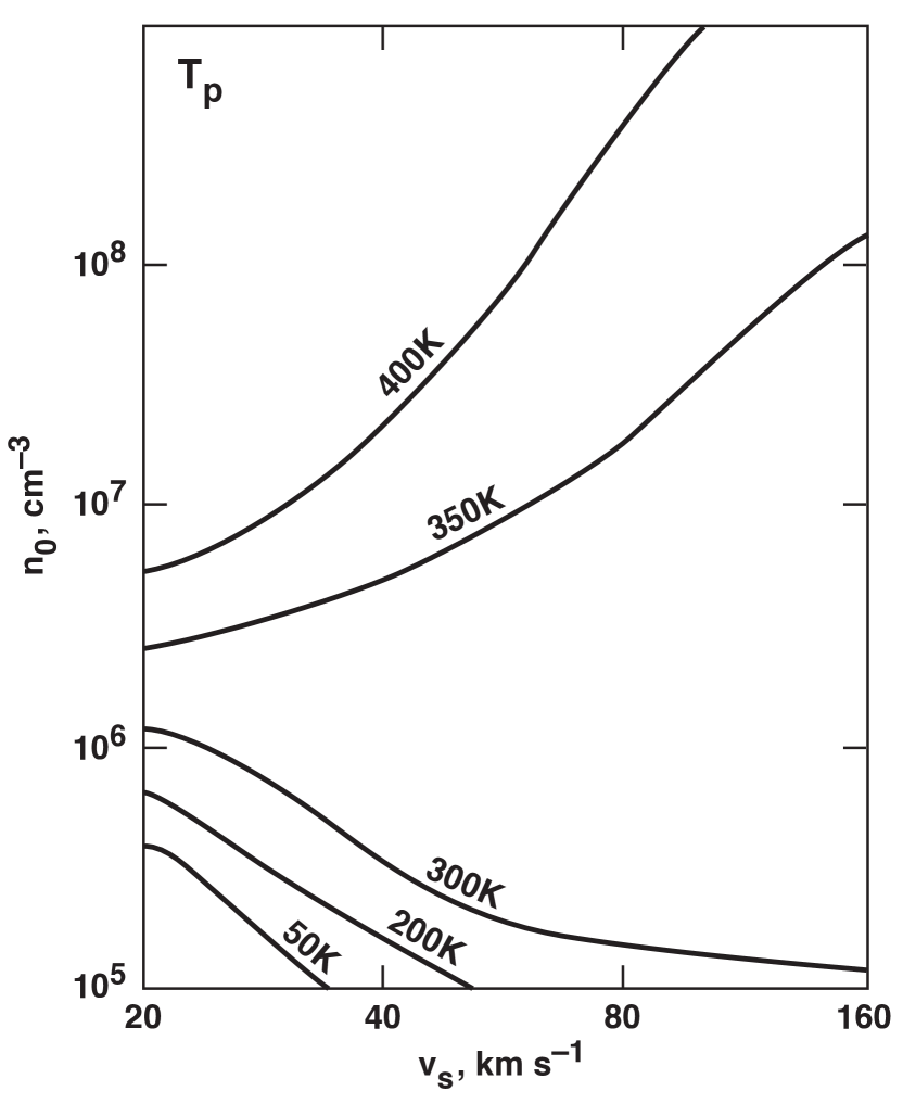
Figure 5: Contours of the gas temperature $T_{p}$ of the plateau region as a function of $n_{0}$ and $v_{s}$. $T_{p}$ is defined as the temperature when 75% of the hydrogen has been re-formed into molecular H₂ [i.e., $x({\rm H_{2}})=0.375$]. For $n_{0}\,\raise 1.29167pt\hbox{$>$}\kern-7.5pt\lower 3.01385pt\hbox{$\sim$}\,10^{5}$ cm^-3, $T_{p}\simeq 350$ K, and is quite insensitive to $n_{0}$ or $v_{s}$ (this is not sufficient for strong maser emission, however—see Fig. 12). For $n_{0}\,\raise 1.29167pt\hbox{$<$}\kern-7.5pt\lower 3.01385pt\hbox{$\sim$}\,10^{5}$ cm^-3, collisional de-excitation of re-forming H₂ in vibrationally-excited states does not occur frequently, and the heating and $T_{p}$ drop.

Figure 5 plots contours of $T_{p}$, the temperature of the H₂ re-formation plateau, as a function of the shock parameters $n_{0}$ and $v_{s}$. The gas temperature declines slightly with $N$ in the H₂ re-formation plateau; we have defined $T_{p}$ as the temperature of the gas when $x$(H₂)=0.375 (i.e., when 75% of the hydrogen is molecular). Figure 5 and the subsequent 3 figures are the results of a grid of shock models ($n_{0}=10^{5},\ 10^{6},\ 10^{7},\ 10^{8}$, and $10^{9}$ cm^-3; $v_{s}=20,\ 40,\ 80,\ 100$, and 160 km s^-1; $v_{A\perp}=1$ km s^-1; $\Delta v_{D}=1$ km s^-1). This grid is sufficiently coarse that the contours are somewhat approximate. As noted above, we have taken $v_{s}=160$ km s^-1 as our upper limit because shocks with $v_{s}\,\raise 1.29167pt\hbox{$>$}\kern-7.5pt\lower 3.01385pt\hbox{$\sim$}\,200$ km s^-1 destroy essentially all of the dust grains. Once there are no grain surfaces upon which to form H₂, molecular re-formation in the postshock gas effectively ceases, no warm H₂O is produced, and postshock H₂O masing action is destroyed. In addition, we have carried out calculations up to $n_{0}=10^{9}$ cm^-3 since dust grains sublimate at higher preshock densities, but in fact maser emission is generally quenched at considerably lower pre-shock densities as discussed above.

The main results from Figure 5 are that $T_{p}\simeq 300-400$ K and that $T_{p}$ is very insensitive to $n_{0}$ and $v_{s}$ as long as $n_{0}\,\raise 1.29167pt\hbox{$>$}\kern-7.5pt\lower 3.01385pt\hbox{$\sim$}\,10^{5}$ cm^-3 and $v_{s}\,\raise 1.29167pt\hbox{$>$}\kern-7.5pt\lower 3.01385pt\hbox{$\sim$}\,30$ km s^-1. EHM discussed this insensitivity as due to the balance between the gas heating by H₂ formation being balanced by H₂O and grain cooling of the gas. An analytic fit to the numerical results gives:

$$T_{p}\simeq 350n_{0,7}^{0.12}v_{s7}^{-0.12}\Delta v_{D5}^{-0.22}\ {\rm K},$$ (3-9)

accurate to a factor of 1.3 for 10⁶ cm${}^{-3}\,\raise 1.29167pt\hbox{$<$}\kern-7.5pt\lower 3.01385pt\hbox{$\sim$}\,n_{0}\,\raise 1.29167pt\hbox{$<$}\kern-7.5pt\lower 3.01385pt\hbox{$\sim$}\,10^{8}$ cm^-3 and 30 km s${}^{-1}\,\raise 1.29167pt\hbox{$<$}\kern-7.5pt\lower 3.01385pt\hbox{$\sim$}\,v_{s}\,\raise 1.29167pt\hbox{$<$}\kern-7.5pt\lower 3.01385pt\hbox{$\sim$}\,160$ km s^-1. For preshock densities $n_{0}\,\raise 1.29167pt\hbox{$<$}\kern-7.5pt\lower 3.01385pt\hbox{$\sim$}\,10^{5}$ cm^-3, the H₂ formation heating rapidly drops because the newly-formed, vibrationally-excited H₂ molecules radiate away their vibrational energy before collisions can transform this excitation energy into heat. However, for $n_{0}\,\raise 1.29167pt\hbox{$>$}\kern-7.5pt\lower 3.01385pt\hbox{$\sim$}\,10^{5}$ cm^-3, the H₂ re-formation plateau provides a temperature environment where the chemical production of H₂O is efficient and where collisional excitation of the 22 GHz H₂O maser, which lies $644$ K above ground, is possible.

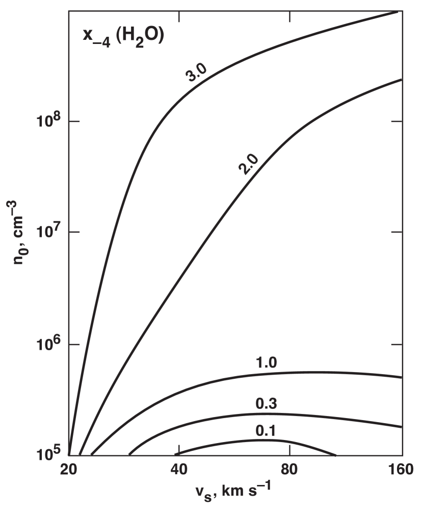
Figure 6: The abundance $x_{-4}({\rm H_{2}O})\equiv x({\rm H_{2}O})/10^{-4}$ is plotted versus $n_{0}$ and $v_{s}$ in the postshock gas at the point where $x({\rm H_{2}})=0.375$, a value near the end of the temperature plateau. For $n_{0}\,\raise 1.29167pt\hbox{$>$}\kern-7.5pt\lower 3.01385pt\hbox{$\sim$}\,10^{5}$ cm^-3, the gas is sufficiently warm and H₂ sufficiently abundant to rapidly drive nearly all the oxygen not in CO into H₂O (this is not sufficient for strong maser emission, however—see Fig. 12).

Figure 6 provides contour plots of the H₂O abundance at the point where $x$(H₂)=0.375 and $x$(H)=0.25, the same position in the re-formation plateau where we measure $T_{p}$. The main result is that an appreciable fraction of the available oxygen is converted to water for $n_{0}\,\raise 1.29167pt\hbox{$>$}\kern-7.5pt\lower 3.01385pt\hbox{$\sim$}\,10^{6}$ cm^-3. At $n_{0}=10^{5}$ cm^-3, the water abundance is only $\sim 10^{-5}$, caused by a combination of lower plateau temperature (see Figure 4) and lower plateau column density $N_{p}$. The former suppresses the rate of H₂O formation because of the activation barriers present in this process. The latter reduces the protective shielding by the dust of the dissociating UV photons, and reduces the time available for H₂O to form. However, for $n_{0}\,\raise 1.29167pt\hbox{$>$}\kern-7.5pt\lower 3.01385pt\hbox{$\sim$}\,10^{6}$ cm^-3, a simple analytic fit to the numerical results gives:

$$x_{-4}({\rm H_{2}O})\simeq 1.6n_{0,7}^{0.2}v_{s7}^{-0.3},$$ (3-10)

accurate to a factor of 1.2 for 10⁶ cm${}^{-3}\,\raise 1.29167pt\hbox{$<$}\kern-7.5pt\lower 3.01385pt\hbox{$\sim$}\,n_{0}\,\raise 1.29167pt\hbox{$<$}\kern-7.5pt\lower 3.01385pt\hbox{$\sim$}\,10^{8}$ cm^-3 and 30 km s${}^{-1}\,\raise 1.29167pt\hbox{$<$}\kern-7.5pt\lower 3.01385pt\hbox{$\sim$}\,v_{s}\,\raise 1.29167pt\hbox{$<$}\kern-7.5pt\lower 3.01385pt\hbox{$\sim$}\,160$ km s^-1.

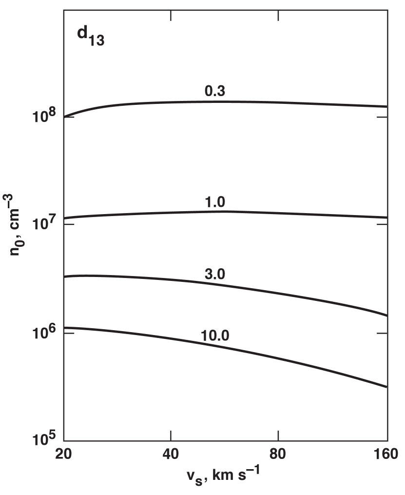
Figure 7: The thickness of the masing region, $d_{13}\equiv d/(10^{13}$ cm), is plotted as a function of $n_{0}$ and $v_{s}$. The parameter $d$ is measured from the shock front downstream to the point where $x({\rm H_{2}})=0.375$. We discuss in text how $d$ is a quite accurate measure of the maser spot size in the dimension parallel to the shock velocity.

The postshock density, $n_{p}$, as a function of $n_{0}$ and $v_{s}$ in the masing plateau is accurately given by the equation in Table 2, and we therefore do not present a contour plot for it. However, $d$ depends on $\gamma_{-17}$ and $\xi$ depends on $\gamma_{-17}$ and $x$(H₂O), and therefore these parameters are accurately determined only by numerical solutions of shock structure. Figure 7 plots the thickness $d_{13}=d/(10^{13}$ cm) of the masing plateau as a function of $n_{0}$ and $v_{s}$. Comparing the numerical results with the equation in Table 2, we see that $\gamma_{-17}$ declines as $n_{0}$ and $v_{s}$ increase, because denser and faster shocks have higher grain temperatures, which reduces the rate of H₂ formation on grain surfaces. In addition, there is reduction in grain area at high values of $n_{0,7}v_{s7}^{3}$ due to partial sublimation of grains. A simple fit to the numerical results gives

$$d_{13}\simeq 1.3n_{0,7}^{-0.7}v_{s7}^{-0.2}v_{A\perp,5}^{2}\ ,$$ (3-11)

$$\gamma_{-17}\simeq 0.38n_{0,7}^{-0.3}v_{s7}^{-0.8},$$ (3-12)

accurate to a factor of 1.5 for 10⁶ cm${}^{-3}\,\raise 1.29167pt\hbox{$<$}\kern-7.5pt\lower 3.01385pt\hbox{$\sim$}\,n_{0}\,\raise 1.29167pt\hbox{$<$}\kern-7.5pt\lower 3.01385pt\hbox{$\sim$}\,10^{8}$ cm^-3 and 30 km s${}^{-1}\,\raise 1.29167pt\hbox{$<$}\kern-7.5pt\lower 3.01385pt\hbox{$\sim$}\,v_{s}\,\raise 1.29167pt\hbox{$<$}\kern-7.5pt\lower 3.01385pt\hbox{$\sim$}\,160$ km s^-1. We note (see also Table 2) that $d\propto v_{A\perp}^{2}$, so that the maser spot size may be the observable parameter that is most sensitive to the strength of the preshock magnetic field. Typical preshock densities of $n_{0,7}\sim 0.1-1$ and observed maser spot sizes of $\sim 10^{13}-10^{14}$ cm imply that $v_{A\perp}\sim 1$ km s^-1, in line with the observations discussed above in Section 3.1.

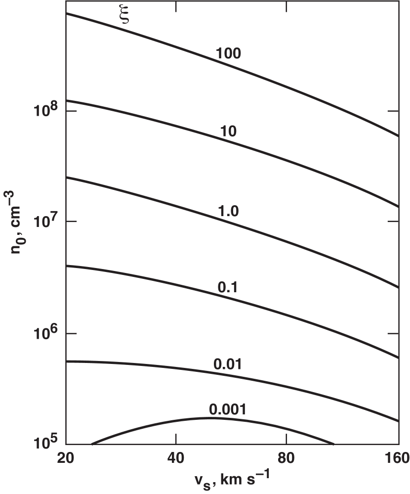
Figure 8: The shock “maser emission measure” $\xi$ is plotted as a function of $n_{0}$ and $v_{s}$. In saturated masers the H₂O maser luminosity and brightness temperature scale as functions of $\xi$ (see text, §2.1), but at high $n_{0}$ the high values of $\xi$ do not lead to bright masers because the inversion can be quenched as the maser levels are driven to LTE.

Figure 8 presents the contours of the maser emission measure $\xi$ [measured from the shock front to the point in the postshock plateau where $x($H${}_{2})$=0.375] as a function of $n_{0}$ and $v_{s}$ for $v_{A\perp,5}$=1 and $\Delta v_{D5}$=1. The main result is that $\xi$ increases monotonically with increasing $n_{0}$, as would be expected from its dependence on the relevant parameters seen in Table 2. From this one might predict that denser masers will be brighter; however, the pump efficiency $\eta$ decreases with increasing $n_{0}$ and ultimately the maser quenches as collisions and line trapping create LTE conditions (see §2). A simple fit to the numerical results gives

$$\xi\simeq 4.0(n_{0,7}v_{s7})^{1.5}\Delta v_{D5}^{-1}=4.0j_{14}^{1.5}\Delta v_{D5}^{-1},$$ (3-13)

accurate to a factor of 1.4 for 10⁶ cm${}^{-3}\,\raise 1.29167pt\hbox{$<$}\kern-7.5pt\lower 3.01385pt\hbox{$\sim$}\,n_{0}\,\raise 1.29167pt\hbox{$<$}\kern-7.5pt\lower 3.01385pt\hbox{$\sim$}\,10^{8}$ cm^-3 and 30 km s${}^{-1}\,\raise 1.29167pt\hbox{$<$}\kern-7.5pt\lower 3.01385pt\hbox{$\sim$}\,v_{s}\,\raise 1.29167pt\hbox{$<$}\kern-7.5pt\lower 3.01385pt\hbox{$\sim$}\,160$ km s^-1.

Utilizing Equations (2-8), (2-9), (3-2), and (3-13) we find good fits to the results of the numerical shock runs for $c_{\eta}$ and $\eta$:

$$c_{\eta}\simeq\left({1+0.045{j_{14}^{2.8}\over{v_{A\perp,5}^{0.2}\Delta v_{D5}^{1.5}}}}\right)^{-1},$$ (3-14)

$$\eta\simeq 0.032{{\Delta v_{D5}^{0.5}c_{\eta}}\over{j_{14}^{0.75}}},$$ (3-15)

which are accurate to within a factor of 1.2 for $c_{\eta}$ and 1.4 for $\eta$ in the parameter range 10⁶ cm${}^{-3}\,\raise 1.29167pt\hbox{$<$}\kern-7.5pt\lower 3.01385pt\hbox{$\sim$}\,n_{0}\,\raise 1.29167pt\hbox{$<$}\kern-7.5pt\lower 3.01385pt\hbox{$\sim$}\,10^{8}$ cm^-3 and 30 km s${}^{-1}\,\raise 1.29167pt\hbox{$<$}\kern-7.5pt\lower 3.01385pt\hbox{$\sim$}\,v_{s}\,\raise 1.29167pt\hbox{$<$}\kern-7.5pt\lower 3.01385pt\hbox{$\sim$}\,160$ km s^-1. The fit to $c_{\eta}$ will be useful in subsequent analytic fits to $a_{\rm sat}$, $d/d_{\perp}$, $T_{b}$ and $L_{\rm iso}$.

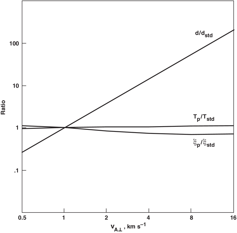
Figure 9: The variation of $d$, $T_{p}$, and $\xi$ as functions of $v_{A\perp}$ is plotted for the standard case (see Fig. 3). The values $d_{\rm std}$, $T_{p,\rm std}$, and $\xi_{\rm std}$ refer to the standard case $v_{A\perp,5}=1$. As predicted (see Section 3.1), $d$ varies as $v_{A\perp}^{2}$, whereas $T_{p}$ and $\xi$ are insensitive to $v_{A\perp}$.

Figures 4-8 are valid for $v_{A\perp,5}=1$, which corresponds with measured values (to within a factor $\sim 6$) for a wide range of cloud densities in the Galaxy. However, as discussed earlier, there may be environments (such as very dense gas or the nuclei of galaxies) where $v_{A\perp,5}$ deviates substantially from unity. Therefore, in Figure 9 we have plotted the variation of $d$, $T_{p}$, and $\xi$ as functions of $v_{A\perp}$ for the standard case $n_{0}=10^{7}$ cm^-3, $v_{s}=100$ km s^-1 and $\Delta v_{D5}=1$. For convenience, we have plotted the ratios of these parameters to their values $d_{\rm std}$, $T_{p,\,\rm std}$, and $\xi_{\rm std}$ at the standard $v_{A\perp,5}$=1. The results follow the predictions from Table 2: $d$ varies as $v_{A\perp}^{2}$ whereas $T_{p}$ and $\xi$ are relatively insensitive to $v_{A\perp}$.

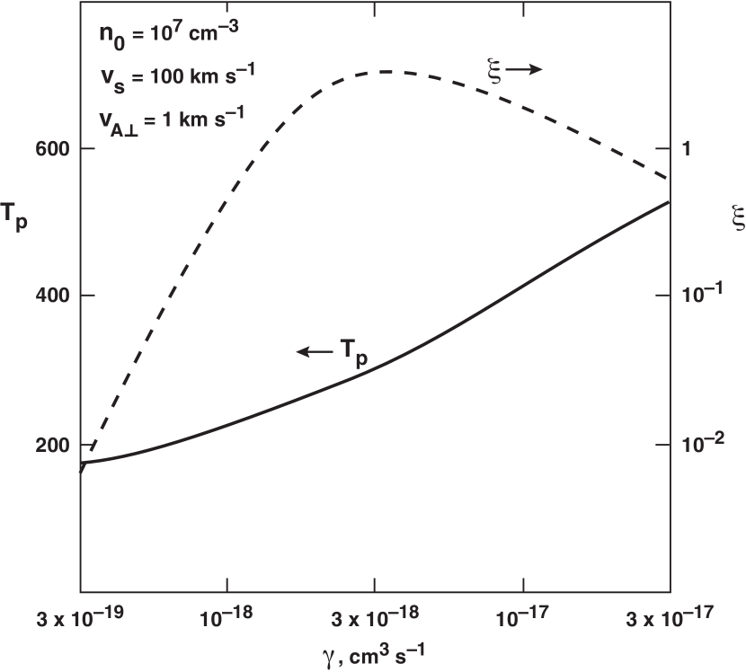
Figure 10: The sensitivity of $T_{p}$ and $\xi$ to the rate coefficient $\gamma$ for H₂ formation. In the parameter study shown in Figures 3 – 8, $\gamma$ is a function of $T$ and $T_{\rm gr}$ (HM79). In this figure, $\gamma$ is held constant in a given run, but varied from $3\times 10^{-19}$ to $3\times 10^{-17}$ cm³ s^-1 over a number of runs. $T_{p}$ is plotted on the left $y$ axis, $\xi$ on the right $y$ axis. All runs assumed the standard parameters $n_{0,7}=v_{s7}=v_{A\perp,5}=1$. These results also test the sensitivity of the model to the assumed heating due to H₂ formation.

Figures 4-9 assume the HM79 model for the formation rate $\gamma$ of H₂ molecules on grains and for the kinetic and rovibrational energy delivered to the gas per H₂ formation. Because the formation process is uncertain, we test the sensitivity of the results to variations in these parameters. Since the heating rate is proportional to the formation rate, we vary only $\gamma$ in this test. In the HM79 model $\gamma$ is a complicated function of gas and grain temperature. Figure 10 presents the results of models with constant $\gamma$ and shows the sensitivity of $T_{p}$ and $\xi$ to variations in $\gamma$. In this figure we test only the standard case ($n_{0,7}=1$, $v_{s7}=1$, $v_{A\perp,5}=1$, and $\Delta v_{D5}=1$). The plateau temperature varies slowly with $\gamma$, changing from 180 K to 550 K as $\gamma$ increases from $3\times 10^{-19}$ cm³ s^-1 to $3\times 10^{-17}$ cm³ s^-1, where the latter corresponds to the maximum H₂ formation efficiency on grains. The emission measure $\xi$ drops rapidly for decreasing $\gamma\,\raise 1.29167pt\hbox{$<$}\kern-7.5pt\lower 3.01385pt\hbox{$\sim$}\,3\times 10^{-18}$ cm³ s^-1, because of the inefficient production of H₂O when the plateau temperature drops below $\sim 250$ K. The water abundance drops from $\sim 3\times 10^{-4}$ for $\gamma\sim 3\times 10^{-18}$ cm³ s^-1 to $\sim 3\times 10^{-7}$ for $\gamma\sim 3\times 10^{-19}$ cm³ s^-1. Therefore, referring to the equation for $\xi$ in Table 2, $\xi\propto x({\rm H_{2}O})/\gamma$ decreases by a factor of $\sim$100 over this range.

4 H₂O MASER SLAB MODELS APPLIED TO SHOCK RESULTS

In §2 we performed a detailed calculation of the H₂O level populations and the radiative transfer in a uniform slab characterized by $\xi$, $n$, and $T$. In §3 we found the values of $\xi$, $n_{p}$ and $T_{p}$ in the H₂ re-formation plateau behind an interstellar J shock as functions of the H nucleus flux into the shock $j=n_{0}v_{s}$, the Alfven speed $v_{A\perp}$, and velocity dispersion in the line-emitting gas $\Delta v_{D}$. In this section we merge the results from these two numerical computations to produce useful predictions concerning the H₂O maser properties of astrophysical J shocks.

4.1 Numerical Results for $a_{\rm sat}$, $d/d_{\perp}$, $T_{b}$, and $L_{\rm iso}$

Perhaps the most important parameter for the application to J-shock models is the aspect ratio of the maser (the ratio of the length along the line of sight to the thickness) required for saturation, $a_{\rm sat}$, which is shown in Figure 11. Shock-produced astrophysical H₂O masers are weak and unobservable as long as they remain unsaturated, so that we shall require $a>\hbox{$a_{\rm sat}$}$. However, the coherence length in the shock plane is finite and $a$ cannot exceed $\sim$ 30–100 because of the curvature of the shock and because of velocity gradients in the plane (e.g., see §5). Therefore, $\hbox{$a_{\rm sat}$}\,\raise 1.29167pt\hbox{$<$}\kern-7.5pt\lower 3.01385pt\hbox{$\sim$}\,30-100$ is a constraint on observable H₂O masers produced in J shocks. Figure 11 shows the dependence of $a_{\rm sat}$ on $n_{0}$ and $v_{s}$ for $v_{A\perp,5}$=1. When $n_{0}\,\raise 1.29167pt\hbox{$<$}\kern-7.5pt\lower 3.01385pt\hbox{$\sim$}\,10^{6}$ cm^-3, $a_{\rm sat}$ rapidly increases to $\,\raise 1.29167pt\hbox{$>$}\kern-7.5pt\lower 3.01385pt\hbox{$\sim$}\,100$ because of the low value of $\xi$ in the shock due to low densities and low values of $x_{-4}({\rm H_{2}O})$. Since such large aspect ratios are extremely unlikely in astrophysical shocks, we conclude that low-density shocks cannot produce saturated masers beamed in the shock plane and that, therefore, such shocks will produce weak, unsaturated masers that are difficult to detect. They are “starved” for sufficient collisions to the highly excited states that feed the maser. At the other extreme, when $n_{0}\,\raise 1.29167pt\hbox{$>$}\kern-7.5pt\lower 3.01385pt\hbox{$\sim$}\,10^{8}$ cm^-3, $a_{\rm sat}$ again rapidly increases to $\,\raise 1.29167pt\hbox{$>$}\kern-7.5pt\lower 3.01385pt\hbox{$\sim$}\,100$ because the maser quenches (levels approach LTE and the inversion is weak) and large coherence paths are needed to reach saturation. At such high preshock densities the plateau density $n_{p}\,\raise 1.29167pt\hbox{$>$}\kern-7.5pt\lower 3.01385pt\hbox{$\sim$}\,4\times 10^{9}$ cm^-3 and $\xi\,\raise 1.29167pt\hbox{$>$}\kern-7.5pt\lower 3.01385pt\hbox{$\sim$}\,10$ (see Table 2 and Figure 8), and therefore quenching is significant (e.g., see $\eta$ in Figure 1 or the quenching of $T_{b}$ at high $\xi$ and $n$ in Figure 3). When $10^{6}$ cm${}^{-3}\,\raise 1.29167pt\hbox{$<$}\kern-7.5pt\lower 3.01385pt\hbox{$\sim$}\,n_{0}\,\raise 1.29167pt\hbox{$<$}\kern-7.5pt\lower 3.01385pt\hbox{$\sim$}\,3\times 10^{7}(v_{A\perp,5}/v_{s7})$ cm^-3 and $0.3\,\raise 1.29167pt\hbox{$<$}\kern-7.5pt\lower 3.01385pt\hbox{$\sim$}\,v_{s7}\,\raise 1.29167pt\hbox{$<$}\kern-7.5pt\lower 3.01385pt\hbox{$\sim$}\,1.6$, $a_{\rm sat}\simeq 1-10$. An analytic fit to $a_{\rm sat}$ can be obtained using Equations (2-11), (3-2), and (3-13) as guides:

$$a_{\rm sat}\simeq 2.5\;{j_{14}^{0.25}\hbox{$\Delta v_{D5}$}^{0.5}\over{v_{A\perp,5}c_{\eta}}},$$ (4-1)

where the expression for $c_{\eta}$ given in Equation (3-14) completes the analytic fit. This expression is good to a factor of 1.3 over the main maser parameter space 10⁶ cm${}^{-3}\,\raise 1.29167pt\hbox{$<$}\kern-7.5pt\lower 3.01385pt\hbox{$\sim$}\,n_{0}\,\raise 1.29167pt\hbox{$<$}\kern-7.5pt\lower 3.01385pt\hbox{$\sim$}\,10^{8}$ cm^-3 and 30 km s${}^{-1}\,\raise 1.29167pt\hbox{$<$}\kern-7.5pt\lower 3.01385pt\hbox{$\sim$}\,v_{s}\,\raise 1.29167pt\hbox{$<$}\kern-7.5pt\lower 3.01385pt\hbox{$\sim$}\,160$ km s^-1.

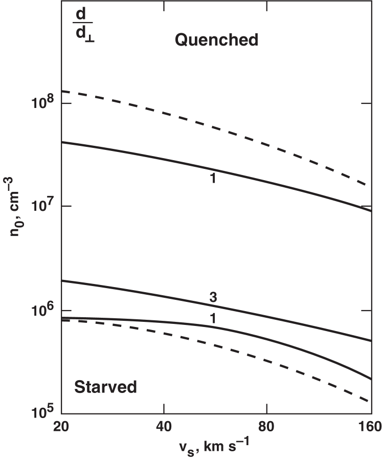
Figure 12: The shape parameter for thin masers (see Appendix B), $d/d_{\perp}$, plotted as a function of $n_{0}$ and $v_{s}$ for $a=10$. Here $d$ is parallel to the shock velocity, and $d_{\perp}$ is perpendicular to the shock velocity and in the plane of the shock. At high preshock densities, $n_{0}\,\raise 1.29167pt\hbox{$>$}\kern-7.5pt\lower 3.01385pt\hbox{$\sim$}\,10^{8}$ cm^-3, the maser is collisionally quenched as levels approach LTE. At low preshock densities, $n_{0}\,\raise 1.29167pt\hbox{$<$}\kern-7.5pt\lower 3.01385pt\hbox{$\sim$}\,10^{6}$ cm^-3, there are too few collisions to excited states to feed the maser (collisionally “starved”). The dashed lines represent $a_{\rm sat}=10$ from Figure 11. Above the top line and below the bottom line, $a_{\rm sat}>10$ and this $a=10$ maser is unsaturated. Here, our equations for $d/d_{\perp}$ fail, and the maser is very weak (see text).

The ratio of the maser spot diameter in the parallel direction to that in the $\perp$ direction, $d/d_{\perp}$, behind J shocks is another observational diagnostic of the shock conditions. The shape $d/d_{\perp}$ of the maser is given in Equations (2-11) and (2-12) in terms of the general parameters $n$, $T$, $\xi$, and $a$. Figure 12 plots $d/d_{\perp}$ for our numerical shock results over the shock parameter space $n_{0}$ and $v_{s}$, assuming $v_{A\perp,5}=1$, $\Delta v_{D5}=1$, and $a=10$. The dashed lines demarcate the zone where $a_{\rm sat}<10$; above the top dashed line and below the lower dashed line $a_{\rm sat}>10$. Our expressions for $d/d_{\perp}$ are no longer valid if the maser is not saturated and therefore we do not plot $d/d_{\perp}$ outside the dashed lines since $a=10<a_{\rm sat}$ there. We see that $d_{\perp}\sim d$ in the strongly masing region of parameter space. Maser spots will be approximately circular and shocked masers can be approximated by equivalent cylinders of diameter $d$ and length $ad$. However, we predict some variation in the shape of the maser spot. An analytic fit can be obtained using Equations (2-12) and (4-1),

$$\frac{d}{d_{\perp}}\simeq{3.3\over a_{\rm sat}}\simeq 1.3\;{{v_{A\perp,5}c_{\eta}}\over j_{14}^{0.25}\hbox{$\Delta v_{D5}$}^{0.5}},$$ (4-2)

good to a factor of 1.5 over the main maser parameter space 10⁶ cm${}^{-3}\,\raise 1.29167pt\hbox{$<$}\kern-7.5pt\lower 3.01385pt\hbox{$\sim$}\,n_{0}\,\raise 1.29167pt\hbox{$<$}\kern-7.5pt\lower 3.01385pt\hbox{$\sim$}\,10^{8}$ cm^-3 and 30 km s${}^{-1}\,\raise 1.29167pt\hbox{$<$}\kern-7.5pt\lower 3.01385pt\hbox{$\sim$}\,v_{s}\,\raise 1.29167pt\hbox{$<$}\kern-7.5pt\lower 3.01385pt\hbox{$\sim$}\,160$ km s^-1 as long as $a>a_{\rm sat}$. Note that if $a>10$, then the dashed lines move to accompany the slightly more allowed $n_{0}$, $v_{s}$ parameter space (see Figure 11). The equation shows that the elongation of the maser in the direction of the shock velocity is directly proportional to the Alfven speed in the ambient medium.

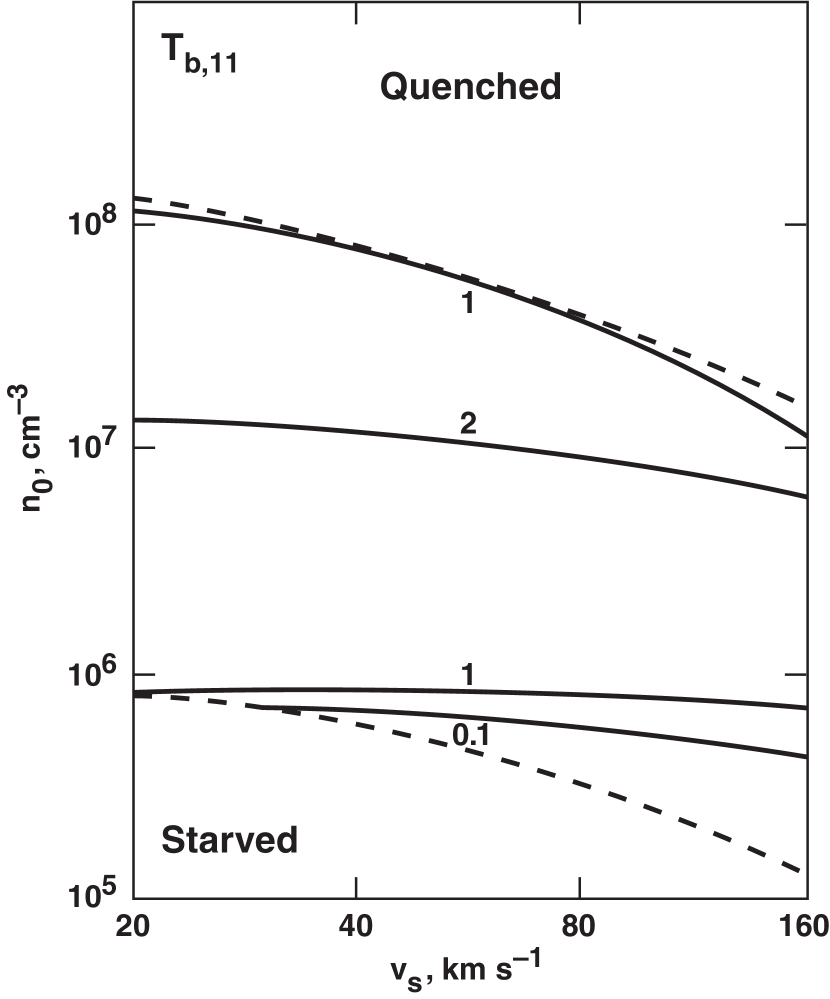
Figure 13: The brightness temperature, $T_{b,11}\equiv T_{b}/(10^{11}$ K), is plotted versus $n_{0}$ and $v_{s}$ for $a=10$. The dashed lines represent $a_{\rm sat}=10$ (Figure 11), so that the $a=10$ maser is unsaturated and $T_{b}$ falls extremely rapidly outside them. Note that these boundaries would expand somewhat (see Figure 11) for $a>10$ since that would allow larger values of $a_{\rm sat}$. We assume in this figure that $v_{A\perp}=1$ km s^-1 and $\Delta v_{D}=1$ km s^-1. The brightness temperature $T_{b}$ scales as $v_{A\perp}\Delta v_{D}^{-1/2}a^{3}$ (see Table 3) for saturated masers.

Figure 13 shows the dependence of $T_{b,11}=T_{b}/(10^{11}$ K) on $n_{0}$ and $v_{s}$ for $v_{A\perp,5}=1$, $\Delta v_{D5}=1$, and $a=10$. The dashed lines are the same as in Figure 12. Since this figure applies to $a=10$, regions outside the dashed lines with $a_{\rm sat}>10$ will have exponentially reduced $T_{b}$ (see Eq. B13) since they will be unsaturated. The effect of entering the unsaturated regime is seen in Figure 3, where very small changes in $\xi$ lead to extremely large changes in $T_{b}$. For $n_{0}\,\raise 1.29167pt\hbox{$<$}\kern-7.5pt\lower 3.01385pt\hbox{$\sim$}\,10^{6}$ cm^-3 the maser is unsaturated and “starved” for exciting collisions as discussed above. For $n_{0}\,\raise 1.29167pt\hbox{$>$}\kern-7.5pt\lower 3.01385pt\hbox{$\sim$}\,3\times 10^{7}(v_{A\perp,5}/v_{s7})$ cm^-3 in the case of $a=10$, the maser is rapidly quenched and $T_{b}$ precipitously drops. For intermediate densities, where the maser is saturated ($a>a_{\rm sat}$), an approximate analytic fit (using Eqs. 2-13, 3-13, and 4-2) to these numerical results is

$$T_{b,11}\simeq 2.5j_{14}^{0.5}\left({v_{A\perp,5}\over\Delta v_{D5}}\right)c_{\eta}^{2}a_{1}^{3}\ {\rm K},$$ (4-3)

which is accurate to a factor of 1.4 for $10^{6}$ cm${}^{-3}\,\raise 1.29167pt\hbox{$<$}\kern-7.5pt\lower 3.01385pt\hbox{$\sim$}\,n_{0}\,\raise 1.29167pt\hbox{$<$}\kern-7.5pt\lower 3.01385pt\hbox{$\sim$}\,10^{8}$ cm^-3 and 30 km s${}^{-1}\,\raise 1.29167pt\hbox{$<$}\kern-7.5pt\lower 3.01385pt\hbox{$\sim$}\,v_{s}\,\raise 1.29167pt\hbox{$<$}\kern-7.5pt\lower 3.01385pt\hbox{$\sim$}\,160$ km s^-1. Note that as long as $c_{\eta}$ is of order unity, that is, as long as $\xi$ and $n$ are not so large that the maser quenches, $T_{b}$ increases with increasing $j$ and/or increasing $v_{A\perp}$. However, if $j$ becomes too large, the maser quenches, $c_{\eta}$ plummets, and $T_{b}$ drops. Although raising $v_{A\perp}$ for fixed $a$ raises $T_{b}$, increasing $v_{A\perp}$ also has the effect of increasing $d$; observed maser spot sizes limit the size of $d$, thereby limiting the possible $v_{A\perp}$ and therefore $T_{b}$ in the region. In addition, since $a=2\ell/d$, increasing $d$ can lower $a$; this then can lead to lower $T_{b}$ even as $v_{A\perp}$ and $d$ increase.

Ever since the detailed study of W51 by Genzel et al. (1981), maser spot sizes have been shown to be uncorrelated with brightness temperature, a finding reaffirmed by the thorough investigation of W49 by Gwinn, Moran & Reid (1992) and Gwinn (1994b). Figure 13 indicates this lack of correlation for fixed $v_{A}$. The brightness temperature does not vary much in the strong masing region, even though (see Figure 7) $d$ varies by a factor of roughly 20 from $\sim 5\times 10^{12}$ cm at the upper boundary to $\sim 10^{14}$ cm at the lower boundary. In addition, note that Figure 13 is for fixed $a=10$. $T_{b}$ varies with $a^{3}$ and therefore the $T_{b}$ spread in a given source arises mostly from variations in $a$. In summary, at fixed $v_{A}$ the brightness is practically independent of the observed dimensions and dependent almost entirely on $a$, in agreement with observations. One can increase $T_{b}$ and $d$ by holding $j$, $a$ and $\Delta v_{D5}$ fixed, but increasing $v_{A}$. In this case, $T_{b}\propto v_{A}\propto d^{1/2}$. Here, there is a weak dependence of $T_{b}$ on $d$, but the very strong dependence on the aspect ratio ($T_{b}\propto a^{3}$) likely washes this out.

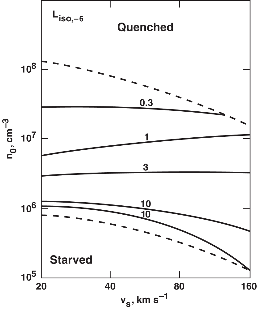
Figure 14: The “isotropic” luminosity, $L_{\rm iso,-6}\equiv L_{\rm iso}/(10^{-6}$ $L_{\odot})$, of the 22 GHz maser is plotted against $n_{0}$ and $v_{s}$ for the standard values $v_{A\perp}=1$ km s^-1, $\Delta v_{D}=1$ km s^-1, and $a=10$. The dashed lines represent $a_{\rm sat}=10$, so that the $a=10$ maser plotted here is unsaturated outside them, and $L_{\rm iso}$ falls rapidly there.

Figure 14 plots the contours of $L_{\rm iso,-6}\equiv L_{\rm iso}/(10^{-6}$ $L_{\odot})$ as a function of $n_{0}$ and $v_{s}$ for our standard values of $v_{A\perp,5}=1$, $\Delta v_{D5}=1$, and $a=10$. The dashed lines are the same as in Figures 12 and 13 (i.e., they demarcate $a_{\rm sat}=10$). For a fixed aspect ratio, the luminosity peaks at somewhat lower $n_{0}$ compared with $T_{b}$ because $L_{\rm iso}/T_{b}$ is proportional to $d^{2}$, and $d$ increases as $n_{0}$ decreases (see Table 2 or Fig. 7). Using Equation (2-15) and the analytic fits (3-13) for $\xi$ and (4-2) for $d/d_{\perp}$, we find a fit for $a>a_{\rm sat}$:

$$L_{\rm iso,-6}\simeq 2.2\left({{v_{s7}v_{A\perp,5}^{4}\Delta v_{D5}^{0.5}c_{\eta}}\over{j_{14}^{0.65}}}\right)a_{1}^{3},$$ (4-4)

which is accurate to a factor of 2 for $10^{6}$ cm${}^{-3}\,\raise 1.29167pt\hbox{$<$}\kern-7.5pt\lower 3.01385pt\hbox{$\sim$}\,n_{0}\,\raise 1.29167pt\hbox{$<$}\kern-7.5pt\lower 3.01385pt\hbox{$\sim$}\,10^{8}$ cm^-3 and 30 km s${}^{-1}\,\raise 1.29167pt\hbox{$<$}\kern-7.5pt\lower 3.01385pt\hbox{$\sim$}\,v_{s}\,\raise 1.29167pt\hbox{$<$}\kern-7.5pt\lower 3.01385pt\hbox{$\sim$}\,160$ km s^-1. Recalling that $j=n_{0}v_{s}$, we see that $L_{\rm iso}$ is proportional to $n_{0}^{-0.65}v_{s7}^{0.35}a_{1}^{3}$ as long as $c_{\eta}$ is of order unity. Therefore, for fixed aspect ratio $a$, the luminosity increases with decreasing preshock density due to the increase in $d$, as discussed above. In addition, regions with high preshock magnetic fields (i.e., high $v_{A\perp}$) will produce much more luminous maser spots, because the maser spot size $d\propto v_{A\perp}^{2}$. In both cases the masers will not be much brighter, but bigger and more luminous. However, there is a very important caveat to this discussion. Recall that the aspect ratio $a=2\ell/d$, the coherence path length divided by the shock thickness. Therefore, as $d$ gets larger, it is likely that $a$ gets smaller. In both Figures 13 for $T_{b}$ and Figure 14 for $L_{\rm iso}$, $a$ is held constant, even as $d$ increases from roughly $3\times 10^{12}$ cm at $n_{0}\sim 10^{8}$ cm^-3 to $10^{14}$ cm at $n_{0}\sim 10^{6}$ cm^-3. This implies that the coherence length is assumed to increase by a factor of roughly 30 as $n_{0}$ decreases over this range. This is likely not physically plausible; $\ell$ will not exactly scale as $d$, and, in fact, $a$ will likely decrease as $d$ increases. Both $T_{b}$ and $L_{\rm iso}$ scale with $a^{3}$. Therefore, the regions of higher preshock density may be more likely to give larger $T_{b}$ and $L_{\rm iso}$.

All the equations derived in this subsection assume that the shocked slab is geometrically thin, that is, $d<\hbox{$d_{\rm thin}$}$ (see §2.3, Table 1, and Eqs. B7 and B8). In this case, the maser spot size observed in the parallel direction is $d$, that is, it is limited by the thickness of the masing region–it is ”matter” bounded. In Appendix C we justify this assumption, using the approximate analytic formulae we have derived. The equations in this section also assume the ${\rm H_{2}}$ formation rate coefficient, $\gamma$, determined by HM79. As discussed at the end of Section 3.3, the value of $\gamma$ has a significant effect on the shock structure. For example, if $\gamma$ drops from $3\times 10^{-18}\;{\rm cm^{3}~{}s^{-1}}$ to $3\times 10^{-19}\;{\rm cm^{3}~{}s^{-1}}$, Table 2 shows that this decrease in $\gamma$ leads to a decrease in the brightness temperature by a factor of $\sim 30$ when we include the $T_{p}$ dependence. On the other hand, the maser spot size $d$ increases by a factor of 10; as a result, for a fixed aspect ratio $a$, the isotropic luminosity $L_{\rm iso}$, which is proportional to $d^{2}T_{b}$, actually increases by a factor of $\sim 3$ for this decrease in $\gamma$. This increase in the maser luminosity is primarily due to the increased area of the maser spot and the increased length of the coherence path $2\ell$ associated with the assumption of a constant aspect ratio.

4.2 Summary of Results for H₂O Masers Produced By Fast J Shocks

We summarize the approximate analytic fits to the numerical results of §2, §3 and §4 in two tables. Table 3 presents the fits to the parameters $d$, $\gamma$, $\xi$, $T_{p}$, $x_{-4}$(H₂O), $c_{\eta}$, $\eta$, $a_{\rm sat}$, $d/d_{\perp}$, $T_{b}$ and $L_{\rm iso}$ as functions of $j=n_{0}v_{s}$, $v_{s}$, $v_{A\perp}$, $\Delta v_{D}$ and $a$. The fits are good to better than a factor of 2 (see Section 4.1 for the individual error estimates) over the range 10⁶ cm${}^{-3}\,\raise 1.29167pt\hbox{$<$}\kern-7.5pt\lower 3.01385pt\hbox{$\sim$}\,n_{0}\,\raise 1.29167pt\hbox{$<$}\kern-7.5pt\lower 3.01385pt\hbox{$\sim$}\,10^{8}$ cm^-3 and 30 km s${}^{-1}\,\raise 1.29167pt\hbox{$<$}\kern-7.5pt\lower 3.01385pt\hbox{$\sim$}\,v_{s}\,\raise 1.29167pt\hbox{$<$}\kern-7.5pt\lower 3.01385pt\hbox{$\sim$}\,160$ km s^-1, which is the range that produces strong J-shock H₂O masers.

Table 4 inverts the equations in Table 3 so that the shock parameters $n_{0}$, $v_{s}$, $j$, $B_{0\perp}$ or $v_{A\perp}$ and $a$ are derived in terms of the potential observables $v_{A\perp}$ or $B_{0\perp}$, $d$, $d/d_{\perp}$, $B_{p}$, and either $T_{b}$ or $L_{\rm iso}$. We also give an expression for $c_{\eta}$ since it is needed in the expression for $a$. It may be the case that $v_{A\perp}$ is not directly observable, but that a rough estimate of $n_{0}$ can be obtained. In this case we can use

$$v_{A\perp,5}\simeq n_{0,7}^{0.45}d_{13}^{0.5}B_{p}^{0.1},$$ (4-5)

which is obtained by inverting the expression for $n_{0,7}$ given in the top line of Table 4. Recall $B_{p}$ is measured in Gauss. Note the weak dependence on $n_{0}$ and especially $B_{p}$, which enables an estimate of $v_{A\perp}$ even when $n_{0}$ is only roughly estimated and $B_{p}$ is even more uncertain.

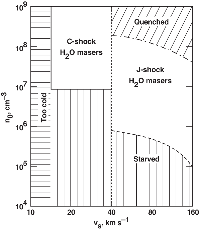
Figure 15: The parameter space ($n_{0}$, $v_{s}$) that produces J-shock masers is shown. For velocities $v_{s}\,\raise 1.29167pt\hbox{$<$}\kern-7.5pt\lower 3.01385pt\hbox{$\sim$}\,40$ km s^-1, the shock is likely not a J shock but a C shock (left of dotted vertical line). This boundary could be at lower $v_{s}$ if the ionization fraction in the preshock gas exceeds $\sim 10^{-7}$. Likewise, the low-velocity boundary of C shocks marked “too cold” could be at lower values of $v_{s}$ if the ionization fraction is higher (see text). J shocks with $v_{s}\,\raise 1.29167pt\hbox{$<$}\kern-7.5pt\lower 3.01385pt\hbox{$\sim$}\,15$ km s^-1 are too cold to form masers, because they do not destroy sufficient H₂ to form a significant warm plateau heated by H₂ re-formation. For velocities $v_{s}\,\raise 1.29167pt\hbox{$>$}\kern-7.5pt\lower 3.01385pt\hbox{$\sim$}\,160$ km s^-1, the shock will significantly destroy grains, which prevents the re-formation of H₂ in the postshock gas and the production of warm H₂O. For preshock densities $n_{0}\,\raise 1.29167pt\hbox{$<$}\kern-7.5pt\lower 3.01385pt\hbox{$\sim$}\,10^{6}$ cm^-3 in J shocks and $\,\raise 1.29167pt\hbox{$<$}\kern-7.5pt\lower 3.01385pt\hbox{$\sim$}\,10^{7}$ cm^-3 in C shocks the masing region requires extremely high aspect ratios, $a\,\raise 1.29167pt\hbox{$>$}\kern-7.5pt\lower 3.01385pt\hbox{$\sim$}\,100$, in order to saturate and become bright enough to detect. For densities $n_{0}\,\raise 1.29167pt\hbox{$>$}\kern-7.5pt\lower 3.01385pt\hbox{$\sim$}\,10^{8}$ cm^-3 in J shocks, the postshock densities and optical depths are so high that the maser level thermalizes, and the inversion is quenched.

Figure 15 graphically plots the J-shock parameter space that produces strong 22 GHz H₂O masers, and indicates the physical mechanisms that intercede to reduce maser activity in J shocks. Above $n_{0}\,\raise 1.29167pt\hbox{$>$}\kern-7.5pt\lower 3.01385pt\hbox{$\sim$}\,10^{8}$ cm^-3, the maser inversion is quenched in J shocks by the high densities and high optical depths in the H₂O infrared transitions, which drive the H₂O rotational levels to LTE and reduce the inversion in the maser levels. Below about $n_{0}\sim 10^{6}$ cm^-3, masers with $a\,\raise 1.29167pt\hbox{$<$}\kern-7.5pt\lower 3.01385pt\hbox{$\sim$}\,10-100$ are weak and unsaturated (“starved”).

Above $v_{s}\,\raise 1.29167pt\hbox{$>$}\kern-7.5pt\lower 3.01385pt\hbox{$\sim$}\,200$ km s^-1, the J shocks destroy most of the dust grains, leaving no grain surface upon which H₂ can reform. As a result, insufficient columns of warm H₂O are produced in the postshock gas, and no observable H₂O masers are excited.

For $v_{s}\,\raise 1.29167pt\hbox{$<$}\kern-7.5pt\lower 3.01385pt\hbox{$\sim$}\,40$ km s^-1, C shocks rather than J shocks may form in dense molecular gas (cf., Draine & McKee 1993, and references therein). We have marked the boundary of C shocks with J shocks with a dashed vertical line in Figure 15 at $v_{s}=40$ km s^-1. This is appropriate if the gas is weakly ionized (ionization fractions of $\,\raise 1.29167pt\hbox{$<$}\kern-7.5pt\lower 3.01385pt\hbox{$\sim$}\,10^{-7}$), so that charged grains mediate the C shock. However, if the dense preshock gas is more highly ionized, perhaps by the UV photons from nearby faster J shocks, this boundary between C and J shocks moves to lower values of $v_{s}$, and the J-shock maser parameter space is extended to lower $v_{s}$. For example, for ionization fractions of about $10^{-5}$ the boundary between J and C shocks occurs near $v_{s}\sim 10$ km s^-1 (Smith & Brand 1990). To the left of the solid line ($v_{s}\,\raise 1.29167pt\hbox{$<$}\kern-7.5pt\lower 3.01385pt\hbox{$\sim$}\,15$ km s^-1, marked “too cold”), no H₂ re-formation plateau is produced in J shocks because too few preshock H₂ molecules are dissociated in J shocks.

4.3 J-Shock Masers Versus C-Shock Masers

Figure 15 also roughly indicates the region of parameter space where C shocks may produce water masers. Kaufman & Neufeld (1996) model H₂O maser emission from such C shocks. Here, the H₂ is not dissociated, but is kept warm over a large column by the ambipolar heating of the neutrals as they drift through the ions. In non-dissociating C shocks, the low density boundary (marked by solid horizontal line at $n_{0}=10^{7}$ cm^-3) is at a higher density than in J shocks because of less compression of the gas in the warm region. Similarly, the upper boundary marked by quenching is raised in C shocks to $n_{0}\sim 10^{9}$ cm^-3.

Several constraints bound the velocity range of C shock masers. For C shocks with low ionization fraction, the postshock peak temperatures are too cold to excite the maser for $v_{s}\,\raise 1.29167pt\hbox{$<$}\kern-7.5pt\lower 3.01385pt\hbox{$\sim$}\,15$ km s^-1. However, for higher ionization fractions, C shocks are warm enough to excite maser emission at shock velocities as low as $v_{s}\sim 5$ km s^-1. Another factor affecting the low-velocity boundary of C-shock masers is the velocity required to sputter water-ice mantles off the grains. The C-shock masers occur in regions of high density, $n_{0}\,\raise 1.29167pt\hbox{$>$}\kern-7.5pt\lower 3.01385pt\hbox{$\sim$}\,10^{7}$ cm^-3, and the freeze-out times for gas phase molecules is very short, $\,\raise 1.29167pt\hbox{$<$}\kern-7.5pt\lower 3.01385pt\hbox{$\sim$}\,100$ years. The grains are likely warm enough to thermally desorb CO, but may not be warm enough ($T_{gr}\,\raise 1.29167pt\hbox{$<$}\kern-7.5pt\lower 3.01385pt\hbox{$\sim$}\,100$ K) to prevent the formation of water-ice mantles. In addition, the FUV radiation fields may sufficiently attenuated to prevent photodesorption of the ice. Therefore, for C shocks to produce strong water maser emission, they must sputter the ice mantles off the grains in these regions, and Draine (1995) estimates that only 10% of the water ice is sputtered off by C shocks with $v_{s}=20$ km s^-1. Hence, unless the radiation field in the C-shock maser region is high enough to warm the grains to $T_{gr}\,\raise 1.29167pt\hbox{$>$}\kern-7.5pt\lower 3.01385pt\hbox{$\sim$}\,100$ K, C shocks must have $v_{s}\,\raise 1.29167pt\hbox{$>$}\kern-7.5pt\lower 3.01385pt\hbox{$\sim$}\,20$ km s^-1 to produce strong water-maser emission. As noted above in our discussion of J shocks, the high-velocity boundary for C shocks also depends on the ionization fraction in the gas, and is likely of order $v_{s}\,\raise 1.29167pt\hbox{$<$}\kern-7.5pt\lower 3.01385pt\hbox{$\sim$}\,30-50$ km s^-1.

Are most water masers produced in J shocks or in C shocks? This is a difficult question to answer with certainty. One measure might be the ram pressure $\propto n_{0}v_{s}^{2}$ needed to drive masing shocks. C shocks require lower shock velocities but higher preshock densities than J shocks. As seen in Figure 15, these two effects roughly cancel each other, suggesting J shocks and C shocks require roughly the same driving pressure and, thus, from this point of view, could be equally likely. However, there may be more gas in the density range that can produce J-shock masers than in the higher density range required for C-shock masers, which would favor J shocks. Water masers require densities of $\sim 10^{8}-10^{9}$ cm^-3. Regions of this density are rare, especially at distances $\,\raise 1.29167pt\hbox{$>$}\kern-7.5pt\lower 3.01385pt\hbox{$\sim$}\,100$ AU from a central protostar along the jet axis, where many masers are observed. The maser emission from C shocks must come from gas that is close to this density, whereas the emission from J shocks comes from gas that has been compressed from a density (only) $\sim 10^{6}-10^{7}$ cm^-3. Another factor to consider is the relative values of the key maser parameter $\xi$, which is proportional to the product of warm postshock column $N_{p}$ times postshock density $n_{p}$. J shocks not only have the advantage in producing higher postshock densities for a given preshock density, as discussed above, but J shocks also produce larger columns of warm gas. In J shocks, the column is determined by the time to reform H₂ in the postshock gas, and $N_{p}\sim 10^{22}$ cm^-2, as we have shown. In C shocks the warm column is determined by the column needed for ions to collide with neutrals and drag the neutrals up to the shock speed. In dense regions, the ionization fraction is low and small charged grains mediate the C shock. The warm coupling column here is only $N_{p}\sim 10^{21}$ cm^-2 (e.g., Kaufman & Neufeld 1996). If gas ions dominate rather than charged grains, the column is even smaller. The smaller value of $N_{p}$ results in a smaller value of $\xi$ and therefore of $T_{b}$ and $L_{\rm iso}$, both of which vary as $\xi^{1/2}$ (Eqs. 2-13 and 2-15).

Another method of distinguishing between the two types of shocks would be to infer the shock velocity, with the idea that slower masers might be C-shock masers. However, in shock masers the maser is beamed perpendicular to the shock velocity (in the plane of the shock). Therefore, even if the shock velocity is high, the Doppler velocity observed will be low. Proper motion studies are needed to try to estimate the shock velocity. Unfortunately, these studies determine the velocity of the shocked gas, not of the shock itself. For example, if high-velocity gas containing dust grains impacts a stationary dense clump or a protoplanetary disk and produces a J shock, the postshock gas would be decelerated to a speed similar to that of the dense gas, resulting in a small proper-motion velocity. The contrary could also occur: if the observed masing gas had a high velocity, one cannot be sure that the maser was induced by J shocks since the emission could originate in fast moving clumps with slow C shocks moving through them. In short, it is difficult to distinguish J-shock masers from C-shock masers by velocity information alone.

Liljestrom & Gwinn (2000) observed 146 maser spots in W49N in the 22 GHz water maser line. Although no attempt was made to compare their observations with C-shock models, they found good agreement with our J-shock models, inferring shock velocities of order 30-100 km s^-1 and aspect ratios of 30-50. In addition, their inferred values of $T_{p}$ and $d$ matched the predictions of J-shock maser models. Many of their masers features had Doppler velocities in excess of 30 km s^-1 and up to $\pm 200$ km s^-1, again suggesting, but not proving, that the masers were produced by J shocks.

J-shock masers might be distinguished by their atomic and ionic infrared line emission. The shocks producing the maser spots likely have typical sizes of order the masing region, or $\,\raise 1.29167pt\hbox{$>$}\kern-7.5pt\lower 3.01385pt\hbox{$\sim$}\,100$ AU. This is a lower limit; in massive star-forming regions like W49 the size is likely of order $10^{17}$ cm. The shock area $A_{\rm shk}$ therefore at least $\,\raise 1.29167pt\hbox{$>$}\kern-7.5pt\lower 3.01385pt\hbox{$\sim$}\,10^{30}$ cm^-2 in low mass star-forming regions and could be as high as $10^{34}$ cm^-2 in high mass star-forming regions. The shock is very embedded, so that the emergent cooling lines must lie in the mid to far infrared, so that they can penetrate the high dust extinction. J shocks differ from C shocks in that they create singly ionized and atomic species, which are strong coolants. C shocks are molecular and mainly cool via molecular rotational lines. One observational test of a J-shock origin is therefore to look for strong infrared cooling transitions from atomic or singly ionized species. For example, in our standard model of a J shock with $n_{0}=10^{7}$ cm^-3 and $v_{s}=100$ km s^-1, we find that the luminosities in the [NeII] 12.8 $\mu$m, [FeII] 26 $\mu$m, and [OI] 63 $\mu$m lines are $3.1\times 10^{-5}(A_{\rm shk}/10^{30}{\rm cm^{-2}})$ L_⊙, $2.1\times 10^{-4}(A_{\rm shk}/10^{30}{\rm cm^{-2}})$ L_⊙, and $1.7\times 10^{-3}(A_{\rm shk}/10^{30}{\rm cm^{-2}})$ L_⊙, respectively. Even with an area of $A_{\rm shk}=10^{30}{\rm cm^{-2}}$, these lines can be detected by the Stratospheric Observatory for Infrared Astronomy (SOFIA) in nearby ($\,\raise 1.29167pt\hbox{$<$}\kern-7.5pt\lower 3.01385pt\hbox{$\sim$}\,1$ kpc) maser regions. The angular resolution of SOFIA for these lines may not be sufficient to spatially resolve these lines, but SOFIA has the sensitivity to detect the fluxes from these lines. We note that although the maser lines originate from portions of the shock nearly edge on, the full shock will likely have considerable portions directed along the line of sight, and therefore the shock IR emission lines could be distinguished from background photodissociation (PDR) regions or HII regions by their width or velocity shifts, which will be of order 30-200 km s^-1. The [NeII] 12.8 $\mu$m line can be also observed with high spectral resolution by 8 meter class telescopes from the ground, at least in the nearest ($\,\raise 1.29167pt\hbox{$<$}\kern-7.5pt\lower 3.01385pt\hbox{$\sim$}\,1$ kpc) masing regions. Here, the spatial resolution is roughly 3 times better than the obtained on SOFIA, and this will also help to disentangle the J shock masing region from background PDRs or HII regions. We note, however, that the [NeII] line is very sensitive to the J shock velocity, and is strong only for $v_{s}\,\raise 1.29167pt\hbox{$>$}\kern-7.5pt\lower 3.01385pt\hbox{$\sim$}\,100$ km s^-1.

Finally, one might appeal to ratios of different masing lines to determine the temperature of the masing gas. As discussed in this paper, J-shock masers likely cannot heat the masing gas to temperatures greater than about $T_{p}\sim 400$ K. However, C-shock masers can heat the masing regions to $T_{p}\,\raise 1.29167pt\hbox{$>$}\kern-7.5pt\lower 3.01385pt\hbox{$\sim$}\,1000$ K. As discussed in the Introduction, maser regions as hot as 1000 K will excite not only the 22 GHz maser, but also a number of submillimeter masers (Kaufman & Neufeld 1996). These authors have applied their results to observations of submillimeter masers, which almost certainly are produced by C shocks. However, there are many more regions where only 22 GHz masers are seen (see Introduction), and these masers are likely produced in cooler $T_{p}\sim 400$ K gas. Although this is suggestive of J-shock masers, again the proof is not definitive since C shocks can also produce dense molecular gas with maximum temperatures of about 400 K.

5 Global Luminosity of a Masing Region

Up to this point we have been discussing the maser emission from a single spot. We have often used a planar disk maser as a model that provides a single maser spot for an observer in the plane. The total maser luminosity from the disk, $L_{m}$, includes the emission seen by observers at all orientations with respect to the maser; it is less than the isotropic luminosity, $L_{\rm iso}$, since the emission is confined to solid angle near the plane of the disk. However, it is unlikely that the maser emission is confined to a single region associated with a given maser spot. Astrophysical shock waves generally cover a significant solid angle as measured from the source of the shock, and as a result they are likely to produce many maser spots, as is often observed. It is therefore instructive to adopt a global viewpoint: What is the total maser luminosity, $L_{m,G}$, emanating from a shock that is produced by a given astronomical phenomenon, such as a wind, an accretion flow, a density wave, or an explosion? For a given shock geometry, which in principle can be inferred from the geometry and kinematics of the maser spots, it is possible to predict the global isotropic luminosity of the maser emission, $L_{{\rm iso},G}$. Provided we do not have a special location with respect to the maser, this global isotropic luminosity will be about the same as the total isotropic luminosity of all the observed maser spots.

Consider a shock with an area $A_{\rm shk}$ that produces masing gas with a thickness $d$. The shape of the shock, such as part of a spherical shell, is determined by the mechanism that produced the shock. The total volume of the masing gas is $V_{m,G}=A_{\rm shck}d$. If a fraction $f_{m}$ of this volume is saturated, then the total luminosity of the maser—the global sum of maser spots radiating in all directions permitted by the shock geometry—is

$$L_{m,G}=\Phi_{m}h\nu_{0}f_{m}V_{m,G}$$ (5-1)

where $\Phi_{m}$ is the volume production rate of maser photons (see Equation A9). Using the maser photon production rate per Hz from Equation (A11) and integrating over the line profile, the maser emission per unit area is then

$${\cal L}_{m}\equiv\frac{L_{m,G}}{A_{\rm shk}}=0.075f_{m}\hbox{$\Delta v_{D5}$}\xi^{1/2}c_{\eta}e^{-460/T}~{}~{}~{}\mbox{erg cm${}^{-2}$\ s${}^{-1}$},$$ (5-2)

which improves upon the result given by Maoz & McKee (1998). This expression is quite general, and applies to masers excited by X-rays (Neufeld, Maloney & Conger 1994) as well, provided the appropriate value of $\xi$ for the X-ray heated gas is used. If the medium is turbulent on scales larger than the shock thickness, then $f_{m}$ in this expression should be interpreted as the areal covering factor of the saturated emission. We do not expect significant turbulence on scales smaller than the shock thickness; however, if there were significant density fluctuations on such small scales, our results would not apply. The total maser luminosity is proportional to the area, and is naturally much greater for observable extragalactic masers than for galactic ones.

The maser luminosity is not an observable quantity, however; rather, it is the global isotropic luminosity, $L_{{\rm iso,G}}\equiv 4\pi D^{2}F_{{\rm obs},G}$, that is measurable, where $F_{{obs},G}$ is the total flux measured by an observer from all the spots in a masing region. If the maser emission covers a fraction $C$ of the sky—i.e., if the masing region radiates into a solid angle $\Omega_{\rm em}=4\pi C$, which means that $C$ is also the fraction of random observers who will see the masers from the region—then the average isotropic luminosity in that solid angle is

$$L_{{\rm iso,G}}=\frac{1}{C}\;L_{m,G}=\frac{1}{C}\;{\cal L}_{m}A_{\rm shk}.$$ (5-3)

In general, emission from the masing region will vary with direction inside $\Omega_{\rm em}$, so that the isotropic luminosity inferred by a given observer might differ from the average somewhat. It should be noted that $\Omega_{\rm em}$ differs from the maser beaming angle of a single maser spot, $\Omega=F_{m}/I$, which relates the flux emitted at the maser surface to the intensity of the maser radiation. For example, a sphere has $\Omega_{\rm em}=4\pi$, corresponding to a covering factor of unity, whereas its maser emission can be tightly beamed, with $\Omega\ll 4\pi$. In Appendix B, we show that for a single maser spot $\Omega_{\rm em}/\Omega=A_{m}/A_{\rm obs}$, where $A_{m}$ is the area over which the maser radiation is emitted and $A_{\rm obs}$ is the observed size of the maser. Furthermore, both $\Omega_{\rm em}$ and $\Omega$ differ from the observed angular size of the maser, $\Omega_{\rm obs}=F_{\rm obs}/I=A_{\rm obs}/D^{2}$.

Disks and cylinders are idealized models for maser emission on the micro-scale. Such structures can be produced by large scale flows associated with accretion disks or with shocks driven by winds or explosions. In accretion disks, maser emission can be produced in density-wave shocks (Maoz & McKee 1998) or by X-ray illumination (Neufeld et al 1994). In both cases, the emission is from a ring of gas, and it is generally beamed close to the plane of the disk. If the maser emits into an angle $2\theta_{\rm em}$ above and below the plane, then the maser emission from a ring is concentrated in a solid angle $\Omega_{\rm em}=2\pi\times 2\sin\theta_{\rm em}=4\pi\sin\theta_{\rm em}$, corresponding to a covering factor $C=\sin\theta_{\rm em}$. In the case of a density-wave shock, the emission comes from a ring of vertical thickness $h$; at a radius $R$, the area of the shock is then $A_{\rm shk}=2\pi Rh$. The average isotropic luminosity of such a ring is then

$$L_{{\rm iso,G}} = \left(\frac{2\pi Rh}{\sin\theta_{\rm em}}\right){\cal L}_{m},$$ (5-4)

$$= 1.2\hbox{$\Delta v_{D5}$}\xi^{1/2}c_{\eta}e^{-460/T}\left(\frac{f_{m}R_{18}h_{16}}{\sin\theta_{\rm em}}\right)~{}~{}~{}L_{\odot},$$ (5-5)

where $R_{18}=R/(10^{18}$ cm), etc.; the normalizations have been chosen in conformity with Maoz & McKee (1998). This is the total isotropic luminosity of the ring, including emission from both sides of the disk; the isotropic luminosity corresponding to just one side of the disk (i.e., to either the blue or the red emission) is half this. A given observer may see the emission from the ring as arising from a number of individual spots, which may result from the alignment of different filamentary masers (Kartje, Königl, & Elitzur 1999). However, the time-averaged emission of all the spots at a given velocity should correspond to half the average isotropic luminosity in Equation (5-5).

Outflows and explosions drive shocks that can give rise to maser emission. For a complete spherical shell of radius $R$, the average isotropic luminosity is simply $L_{{\rm iso,G}}=4\pi R^{2}{\cal L}_{m}$. Outflows from protostars and AGN are more likely to produce shocks that extend over only a part of the sky. We approximate such a shock as being part of a spherical shell that subtends a solid angle $\Omega_{\rm shell}=2\pi(1-\cos\theta_{\rm shell})$ as seen from the center of the sphere; the area of the shock is then $A_{\rm shk}=R^{2}\Omega_{\rm shell}$. One can then show that the maser emits into a solid angle $\Omega_{\rm em}=4\pi\sin\theta_{\rm shell}$ for $\theta_{\rm shell}\leq\pi/2$, provided $\theta_{\rm shell}$ is not too small. Observe that for $\theta_{\rm shell}=\pi/2$, the emission fills $4\pi$ sr; thus, a hemisphere emits in all directions. For $\theta_{\rm shell}>\pi/2$, the emission solid angle remains $\Omega_{\rm em}=4\pi$. However, if $\theta_{\rm shell}$ is too small, the beaming is determined by the thickness of the shell rather than its curvature. In this case, the partial shell approaches a disk of radius $\ell=R\theta_{\rm shell}$. If we define the emission angle $\theta_{\rm em}$ through

$$C=\frac{\Omega_{\rm em}}{4\pi}=\sin\theta_{\rm em},$$ (5-6)

which is consistent with the above discussion of emission from a ring, then (for $\theta_{\rm em}=1/(2a)\ll 1$) $\theta_{\rm em}=C=L_{m,G}/L_{{\rm iso,G}}=d/4\ell$ (EHM92). There is a critical value of $\theta_{\rm shell}$ for which $\theta_{\rm em}$ for the disk equals $\theta_{\rm em}=\theta_{\rm shell}$ for the shell; this value is

$$\theta_{\rm sd}\equiv\frac{1}{2}\left(\frac{d}{R}\right)^{1/2}.$$ (5-7)

The beaming is like that due to a disk for $\theta_{\rm shell}<\theta_{\rm sd}$. The maximum size of a disk that can fit into a shell is then $\ell_{\rm max}=R\theta_{\rm sd}=\frac{1}{2}(Rd)^{1/2}$, and the corresponding maximum aspect ratio is $a_{\rm max}=(R/d)^{1/2}$. From Equations (5-3) and (5-6), the average isotropic luminosity of a shell is then

$$L_{{\rm iso,G}} = 2\pi R^{2}\left(\frac{1-\cos\theta_{\rm shell}}{\sin\theta_{\rm em}}\right){\cal L}_{m},$$ (5-8)

$$= 1.2\times 10^{-4}R_{15}^{2}\left(\frac{1-\cos\theta_{\rm shell}}{\sin\theta_{\rm em}}\right)f_{m}\hbox{$\Delta v_{D5}$}\xi^{1/2}c_{\eta}e^{-460/T}~{}~{}~{}L_{\odot}$$ (5-9)

where

$$\theta_{\rm em}=\left\{\begin{array}[]{l}\displaystyle\frac{d}{4\ell}~{}~{}~{}~{}~{}~{}~{}~{}\theta_{\rm shell}<\theta_{\rm sd}=\frac{1}{2}\left(\frac{d}{R}\right)^{1/2}\\ \displaystyle\theta_{\rm shell}~{}~{}~{}~{}~{}\theta_{\rm sd}\leq\theta_{\rm shell}\leq\frac{\pi}{2}\\ \displaystyle\frac{\pi}{2}~{}~{}~{}~{}~{}~{}~{}~{}\frac{\pi}{2}\leq\theta_{\rm shell}\end{array}\right.$$ (5-10)

For $\theta_{\rm shell}\leq\theta_{\rm sd}$ and $f_{m}=1$, this reduces to Equation (2-15) for a disk, as it should. At high resolution, the shell will break up into individual spots with a spatial distribution that reflects the overall geometry of the shell.

As discussed in §4.1, Equation (4-4) for a maser spot can be misleading since the aspect ratio is $2\ell/d$, and $d$ depends on $n_{0}$, $v_{s}$, and $B_{0\perp}$, whereas $\ell$ can depend on other quantities such as the shock curvature $R$. Therefore, $a$ can decrease with increasing $d$, and should not be treated as a constant independent of $d$. The dependence of the isotropic luminosity of an entire masing region on the geometric properties of the source is more clearly shown by the expression for $L_{\rm iso,G}$ in Equation (5-8), which is based on the assumption that the masing gas is part of a spherical shell of radius $R$ that subtends an angle $2\theta_{\rm shell}$ as seen from the center of the sphere:

$$L_{\rm iso,G}\simeq 0.50\times 10^{-4}R_{15}^{2}\left(\frac{1-\cos\theta_{\rm shell}}{\sin\theta_{\rm em}}\right)f_{m}\hbox{$\Delta v_{D5}$}^{0.5}j_{14}^{0.75}c_{\eta}~{}~{}~{}L_{\odot},$$ (5-11)

where $\theta_{\rm em}$ is given by Equation (5-10); recall that $f_{m}$ is the filling factor of the masing gas. If the masing segment of the shell is small [$\theta_{\rm shell}<0.5(d/R)^{1/2}$], then $L_{\rm iso,G}=L_{\rm iso}$ as noted above; for fixed $\ell$, both vary as $1/d$. For the more typical case in which the shell is not small, the global isotropic luminosity is independent of the shell thickness for fixed $j$; it represents the isotropic luminosity of all the maser spots in the source and no longer scales in the same way as the isotropic luminosity of a single maser spot.

We conclude this section with a final point on the aspect ratios that can be achieved in a shocked shell, expanding outwards at velocity $v_{s}$, and with a radius of curvature $R$. There is a geometric limit on $a$ as noted above: If $d$ is the thickness of the shell, then the maximum physical length of the coherence path 2$\ell$ is $(Rd)^{1/2}$ and the maximum velocity coherence length is $R\Delta v_{D}/v_{s}$. As a result, the maximum aspect ratio is

$$a_{\rm max}=\min\left[(\Delta v_{D}/v_{s})(R/d),(R/d)^{1/2}\right]$$ (5-12)

For example, if $\Delta v_{D}=1$ km s^-1 and $v_{s}=50$ km s^-1, then $\Delta v_{D}/v_{s}=2\hbox{$\times$}\hbox{$10^{-2}$}$, an aspect ratio of 50 can be achieved in principle if $d=10^{13}$ cm and $R\simeq 2.5\hbox{$\times$}\hbox{$10^{16}$}$ cm, comparable with the observed sizes of clusters of H₂O 22 GHz maser spots. Note that this limit on $a$ also applies to the case in which two masing filaments are aligned: the total aspect ratio of the combined masing regions cannot exceed this limit if the masers are part of an expanding spherical shell.

6 CONCLUSIONS AND COMPARISON TO OBSERVATIONS

Using a grid of numerical shock models coupled with a grid of slab models for H₂O maser production, we have shown that J shocks in the range $10^{6}$ cm${}^{-3}\,\raise 1.29167pt\hbox{$<$}\kern-7.5pt\lower 3.01385pt\hbox{$\sim$}\,n_{0}\,\raise 1.29167pt\hbox{$<$}\kern-7.5pt\lower 3.01385pt\hbox{$\sim$}\,10^{8}$ cm^-3 and 30 km s${}^{-1}\,\raise 1.29167pt\hbox{$<$}\kern-7.5pt\lower 3.01385pt\hbox{$\sim$}\,v_{s}\,\raise 1.29167pt\hbox{$<$}\kern-7.5pt\lower 3.01385pt\hbox{$\sim$}\,200$ km s^-1 produce strong, saturated, beamed 22 GHz H₂O masers. The masers are generally beamed because the velocity coherence pathlength $2\ell$ in the shock plane is usually greater than the masing pathlength $d$ in the direction of the shock velocity; this beaming is therefore characterized by the aspect ratio $a\equiv 2\ell/d\,\raise 1.29167pt\hbox{$>$}\kern-7.5pt\lower 3.01385pt\hbox{$\sim$}\,1$. The numerical results of the combined shock and maser models are shown in Figures 11-15.

We have also presented useful analytic formulae (Tables 2-4) that show how the observed maser spot size $d$, shape ($d/d_{\perp}$), flux (or isotropic luminosity, $L_{\rm iso}$), and brightness temperature $T_{b}$ scale with the physical parameters in the shock regions ($n_{0}$, $v_{s}$, $v_{A\perp}$, $\Delta v_{D}$, and $a$). In addition we invert these equations so that the observed quantities can be used to derive the physical parameters in the shock region. Table 2 presents analytic equations derived from shock and maser theory, whereas Tables 3 and 4 provide analytic fits to the numerical shock models. We note in Table 3 and §5 that a number of the key parameters ($\xi$, $c_{\eta}$, $\eta$, $a_{sat}$, $d/d_{\perp}$, $L_{{\rm iso,G}}$, and $T_{b}$) depend only on the combination $j=n_{0}v_{s}$, rather than on $n_{0}$ and $v_{s}$ separately. The maser results in all three tables assume that the maser is saturated. A key difference among the tables is that in Table 2 the average values in the maser plateau of $x({\rm H_{2}O})$ and of $\gamma$, the rate coefficient for H₂ formation on grain surfaces, appear in the equations; in Tables 3 and 4 the numerical results for these parameters provided by the shock models are incorporated into the resulting equations, so that these parameters do not appear.

We conclude with a summary of how 22 GHz water maser observations of $T_{b}$, $L_{\rm iso}$, $d$, $d/d_{\perp}$, $B_{p}$, $T_{p}$, $n_{p}$, beaming, maser velocity, and maser transience correspond to the theoretical models described in this paper.

$T_{b}$. Observed 22 GHz maser brightness temperatures range from $T_{b}\sim 10^{11}$ to $10^{14}$ K (e.g., Genzel 1986, Gwinn 1994b). Figure 3 shows that it is impossible for any 400 K slab of gas with an aspect ratio $a=10$ in the plane of the slab to produce brightness temperatures in excess of about $10^{12}$ K. This is independent of whether the slab was produced by shocks, or by some other mechanism. Therefore, to reach brightness temperatures of $10^{14}$ K, either high aspect ratios, $a\,\raise 1.29167pt\hbox{$>$}\kern-7.5pt\lower 3.01385pt\hbox{$\sim$}\,50$ are required, or there must be two masing regions lined up along the line of sight such that their “effective” $a$ is of this order (see Elitzur, McKee & Hollenbach 1991). Figure 13 shows that J shocks characterized by preshock densities roughly in the range $10^{6}$ cm${}^{-3}\,\raise 1.29167pt\hbox{$<$}\kern-7.5pt\lower 3.01385pt\hbox{$\sim$}\,n_{0}\,\raise 1.29167pt\hbox{$<$}\kern-7.5pt\lower 3.01385pt\hbox{$\sim$}\,10^{8}$ cm^-3 and $30$ km s${}^{-1}\,\raise 1.29167pt\hbox{$<$}\kern-7.5pt\lower 3.01385pt\hbox{$\sim$}\,v_{s}\,\raise 1.29167pt\hbox{$<$}\kern-7.5pt\lower 3.01385pt\hbox{$\sim$}\,160$ km s^-1 produce $T_{b}\sim 1-2\times 10^{11}$ K if $a=10$, and require $a\sim 100$ (or again two regions lined up along the line of sight to simulate $a\sim 100$) to produce $T_{b}\sim 10^{14}$ K. Since $d\sim 10^{13}-10^{14}$ cm, an aspect ratio $a=100$ corresponds to a coherence path length of about $10^{15}-10^{16}$ cm. Maser brightness temperatures $T_{b}$ have been observed to be uncorrelated with maser spot size $d$ (Genzel et al 1981; Gwinn, Moran, & Reid (1992), Gwinn (1994b). We have also shown that shock models do not produce a significant correlation of $T_{b}$ with $d$. The dependence of $T_{b}$ on $d$ is very weak, and variations in $T_{b}$ are primarily controlled by the aspect ratio $a$, since $T_{b}\propto a^{3}$.

$L_{\rm iso}$. Observed isotropic 22 GHz maser luminosities range from $\sim 10^{-7}-10^{-1}$ $L_{\odot}$ from individual maser spots in the Galaxy (Genzel & Downes 1977; Walker, Matsakis & Garcia-Barreto 1982; Genzel 1986; Gwinn 1994a). In spatially unresolved maser regions, the global isotropic luminosity $L_{\rm iso,G}$ is higher, since all the spot luminosities are added together. In particular, Genzel & Downes (1977) find that sources with maser spectra classified as “singles” have a mean value of $L_{\rm iso,G}$ of $10^{-5}$$L_{\odot}$. Assuming such spectra to be dominated by one bright maser spot, this would imply $a$ = 18 for the mean aspect ratio of a single feature if we use $d$ = 1AU in Equation (2-15). The mean value of $L_{\rm iso,G}$ increases with the complexity of the source spectrum; this can be attributed to an increase in the number of spots contributing to the overall emission; physically, it is due to an increase in the overall size of the masing region (Eq. 5-8). The exceptionally luminous maser region W49N is a Galactic outlier. With $L_{\rm iso,G}=1.3L_{\odot}$, its brightest spot has $L_{\rm iso}=0.08L_{\odot}$ which is about 8 times the total isotropic luminosity of the most luminous maser sources outside the W49 complex. This outlier status can be attributed to the short lifetime ( $<$$\sim$  1,000 years) of the bright maser phase in high-mass star forming regions (Mac Low et al 1994; Elitzur 1995). Starburst galaxies can be expected to contain more W49-class maser sources, and indeed Brogan et al (2010) find three maser regions in the Antennae interacting galaxies with $L_{\rm iso,G}$ ranging from 1–6 times the W49 luminosity. For the H₂O masers associated with star formation and outflows, the H₂O luminosity is correlated with the mechanical luminosity seen in the CO outflow (Felli, Palagi & Tofani 1992, Claussen et al 1996, Furuya et al 2001). Such a correlation is expected in a shock model; the mass loss produces the shocks that, in turn, produce the masers. Figure 14 shows that in the range of saturated masers with $10^{6}$ cm${}^{-3}\,\raise 1.29167pt\hbox{$<$}\kern-7.5pt\lower 3.01385pt\hbox{$\sim$}\,n_{0}\,\raise 1.29167pt\hbox{$<$}\kern-7.5pt\lower 3.01385pt\hbox{$\sim$}\,10^{8}$ cm^-3 and $30$ km s${}^{-1}\,\raise 1.29167pt\hbox{$<$}\kern-7.5pt\lower 3.01385pt\hbox{$\sim$}\,v_{s}\,\raise 1.29167pt\hbox{$<$}\kern-7.5pt\lower 3.01385pt\hbox{$\sim$}\,160$ km s^-1, the isotropic luminosity $L_{\rm iso}$ ranges from about $3\times 10^{-7}-10^{-5}$ $L_{\odot}$ for $a=10$. To achieve isotropic luminosities as high as 0.08 $L_{\odot}$ would require $a\,\raise 1.29167pt\hbox{$>$}\kern-7.5pt\lower 3.01385pt\hbox{$\sim$}\,200$. Since the $0.08L_{\odot}$ upper limit arose from the extreme case of a maser spot in W49, this spot could correspond to two coherent regions lining up to give an exceptionally high effective $a$. For both $T_{b}$ and $L_{\rm iso}$, we note that the predictions of the model are dependent on the collisional rate coefficients to excite H₂O. These rate coefficients, especially for collisions with atomic H (the H₂ rates are often scaled from theoretical results of He collisions, but H is more reactive than He or H₂), are somewhat uncertain, and larger rate coefficients might also give higher $T_{b}$ and $L_{\rm iso}$ without requiring such exceptionally high values of the aspect ratio, $a$.

$d$. Observed 22 GHz maser spot sizes are of order $10^{13}-10^{14}$ cm (Genzel 1986; Gwinn 1994a; Torrelles et al 2001a,b; Lekht et al 2007; Marvel et al 2008) when the maser is spatially resolved by very long baseline interferometry. Figure 7 shows that this size range falls right in the middle of our optimum J-shock maser range. Relatively bright and luminous maser spots (Figures 13 and 14) are predicted in our standard model to occur when $n_{0}\sim 10^{6}$ cm^-3 if the aspect ratio remains high even as $d$ increases with decreasing $n_{0}$. Since shocks are driven by high pressure (ram or thermal) and the frequency of occurrence of high pressures in the ISM is a decreasing function of pressure, one would expect more masers to be found with $n_{0}=10^{6}$ cm^-3 than with higher preshock densities. However, our standard model predicts these masers to have size $d\sim 10^{14}$ cm, at the upper end of the typical maser size. If most luminous maser spots are smaller, one explanation for this apparent discrepancy is that the aspect ratio $a$ decreases with increasing $d$. This would greatly lower $T_{b}$ and $L_{\rm iso}$ (proportional to $a^{3}$) for masers with preshock density $n_{0}\sim 10^{6}$ cm^-3. The other possibility is that our models have overestimated $d$. Referring to Table 2, we see that $d$ is proportional to $v_{A\perp}^{2}/\gamma$. For our standard shock models, we use $v_{A\perp}=1$ km s^-1 and the H₂ rate coefficient $\gamma$ is taken from the $T$ and $T_{\rm gr}$-dependent formulation given in HM79. If $v_{A\perp}^{2}/\gamma$ is of order 3 times smaller than we have assumed, the typical maser spot size will come more closely in alignment with the observations. In fact, the equation for $d$ in Table 2 predicts that $v_{A\perp,5}^{2}/(\gamma_{-17}j_{14})\sim 6$ for $d\sim 3\times 10^{13}$ cm.

$d/d_{\perp}$. Figure 12 shows that in the main region of saturated 22 GHz masers, $d/d_{\perp}$ in J-shock models lies between 1 and 3. We therefore predict that maser spot shapes are often fairly circular and that masers usually extend in the direction of the shock velocity. Equation (4-2) shows that the shape variation comes mostly from the Alfven speed $v_{A}$, since the dependence of $d/\hbox{$d_{\perp}$}$ on $j$ is rather weak. If the ambient magnetic field is roughly uniform over the maser region, then the shapes of the maser spots will vary primarily due to the variation in the relative orientation of the magnetic field and the shock velocities. Observationally, maser spot sizes are determined from circular-Gaussian fits to spectral features in maps of the correlated flux (e.g., Gwinn 94, Richards et al 2011). Discerning the elongations predicted here would require a more detailed analysis of maser maps that employs elliptical Gaussian fits to individual maser features, and could provide a new method of inferring the properties of regions with ${\rm H_{2}O}$ masers.

$B_{p}$. Fiebig & Güsten (1989) have observed the Zeeman splitting of the 22 GHz H₂O maser in W49 and estimated the component of the B field along the line of sight to be about 100 mG. Sarma et al (2008) and Alves et al (2012) report Zeeman splittings in a high mass star-forming region (OH 43.8-0.1) and a low mass star-forming region (IRAS 1693-2422), respectively, and estimate B fields of 10-20 mG and 100 mG, respectively. The shock model predicts similar values for $B_{p}$ in the masing region (Table 2).

$T_{p}$. The 22 GHz water maser lies 644 K above the ground state of water. Collisional excitation of this maser therefore requires $T\,\raise 1.29167pt\hbox{$>$}\kern-7.5pt\lower 3.01385pt\hbox{$\sim$}\,300$ K. On the other hand, their observed linewidths ($\,\raise 1.29167pt\hbox{$<$}\kern-7.5pt\lower 3.01385pt\hbox{$\sim$}\,1$ km s^-1) suggest thermal temperatures generally $\,\raise 1.29167pt\hbox{$<$}\kern-7.5pt\lower 3.01385pt\hbox{$\sim$}\,1000$ K (Liljestrom & Gwinn 2000). Millimeter observations, the observed 321 GHz H₂O maser (Neufeld & Melnick 1990), and the observation that there are not enough external photons to pump the maser all point to warm gas in the range $300-1000$ K. J shocks produce a large column of H₂O in the lower part of this temperature range, at 300-400 K (see Figure 5), where collisions can pump the 22 GHz maser. However, in some regions, observations of other maser transitions of H₂O indicate higher temperatures than J shocks seem to be able to provide in the H₂ re-formation plateau, and C shocks may be implicated since these shocks can produce higher gas temperatures in an extended molecular column. Kaufman & Neufeld (1996) have modeled such shocks and applied their results to multitransition observations of water masers (Menten, Melnick, & Phillips 1990; Chernicharo et al 1990; Menten et al 1990; Melnick et al 1993).

$n_{p}$. Genzel (1986) reviews observational evidence that the density in the 22 GHz masing region is $\,\raise 1.29167pt\hbox{$>$}\kern-7.5pt\lower 3.01385pt\hbox{$\sim$}\,10^{9}$ cm^-3 (for a recent study, see Alves et al 2012). We see from Figure 3 that any $T=400$ K slab, whether produced by a shock or not, has much lower $T_{b}$ once $n\gg 10^{9}$ cm^-3 because of the quenching of the maser. The beauty of the shock model is that regions of density $n\sim 10^{9}$ cm^-3 are rare, especially $\,\raise 1.29167pt\hbox{$>$}\kern-7.5pt\lower 3.01385pt\hbox{$\sim$}\,100$ AU from a central protostar along the jet axis, where many masers are observed, and the J shock compresses preshock gas of density (only) $\sim 10^{7}$ cm^-3 to this density. We note that C shocks produce much of the maser emission in their warmer regions, which are not nearly as compressed as J shocks. Therefore, C shocks require substantially higher preshock densities (see Figure 15), which may be rarer.

Beaming. As expected from the planar shock geometry, maser radiation is preferentially beamed perpendicular to the motion of the emitting material. This can be inferred indirectly from the inverse correlation between measured Doppler velocity and maser brightness (e.g., Genzel 1986) or from the increased numbers of masers observed with low los velocities compared with high los velocities (e.g., Walsh et al 2011) and directly from spatially resolved observations which show that the maser velocity vectors lie nearly in the plane of the sky (Marvel et al 2008). Beaming angles themselves are immeasurable and can only be inferred indirectly. Gwinn (1994c) has modeled the diffuse H₂O maser “haloes” around maser spots in W49N as arising from scattering by nearby ionized plasma and concluded that the masers are indeed beamed. His analysis suggests that the beaming angles lie in the range 0.002 $\,\raise 1.29167pt\hbox{$<$}\kern-7.5pt\lower 3.01385pt\hbox{$\sim$}\,\theta_{m}\,\raise 1.29167pt\hbox{$<$}\kern-7.5pt\lower 3.01385pt\hbox{$\sim$}\,0.02$ radians, corresponding to aspect ratios $500\,\raise 1.29167pt\hbox{$>$}\kern-7.5pt\lower 3.01385pt\hbox{$\sim$}\,a\,\raise 1.29167pt\hbox{$>$}\kern-7.5pt\lower 3.01385pt\hbox{$\sim$}\,50$. Unfortunately, in the absence of any followup work to verify the assumptions entering into the chain of analysis in this pioneering study, these bounds can only be considered as order-of-magnitude estimates. Aspect ratios of order $\,\raise 1.29167pt\hbox{$<$}\kern-7.5pt\lower 3.01385pt\hbox{$\sim$}\,50$, similar to Gwinn’s lower bound, are expected in our model for single maser features while values of $\sim$200–500 could arise from the alignments of two maser regions (Deguchi & Watson 1989; Elitzur, McKee & Hollenbach 1991), needed to explain the high-end of brightness temperatures ($\sim$$10^{14}$ K). Another indirect determination of the beaming angle is through time monitoring. Using spectroscopic results of 146 water maser outbursts in W49N, Liljeström & Gwinn (2000) derive aspect ratios of 16–28 if the masers are filamentary and 29–52 if they are disks. One big flare stands out with aspect of either 70 or 126, depending on the geometry. All results are consistent with aspect ratios of order a few tens for single maser regions.

Observed maser velocity. As noted above in the discussion on beaming, the masers with low los velocities are brighter. However, when time lapse images show motions in the plane of the sky, we find that, for example in W49 and IRAS 05413-0104, the space velocities are almost always in excess of 25 km s^-1 (Gwinn 1994a, Claussen et al 1998, Liljeström & Gwinn 2000, Marvel et al, 2008). In W75N, 20 years of monitoring show maser speeds of $\sim 75$ km s^-1 (Lekht et al 2007). These speeds are in line with the velocities needed to excite masers in J shocks (see Figure 15), although we note that shocks in the range $v_{s}\sim 20-40$ km s^-1 are likely to be C shocks and not J shocks, unless the ionization fraction is higher than $\sim 10^{-7}$. However, In applying these models to observations, some thought must be given concerning the dependency of the observed line of sight and proper motion velocities of interstellar H₂O masers on the shock velocity $v_{s}$, the wind/jet velocities $v_{w}$ observed in the masing region, and the velocity $v_{a}$ of the ambient gas. In strong J shocks, the flow velocity of the masing gas with respect to the shock front is very slow, $\sim(n_{0}/n_{p})v_{s}\sim 10^{-2}v_{s}$, so that the masing gas moves at $\sim v_{s}$ with respect to the preshock gas. We envisage the shocks that produce H₂O masers as arising when high speed (jet, wind, or a shell or clump driven by the wind) material moving at $v_{w}$ from a protostar interacts with slower “ambient” material moving at $v_{a}$. The ambient material might be either a clump in the ambient molecular gas, a circumstellar disk, or a slowly moving shell of already shocked material (sometimes, this is identified as “outflow” material). In this picture the shock velocity is then $v_{s}\simeq v_{w}-v_{a}$. If the high speed material is denser than the ambient material, then the ambient gas is shocked up to the speed of the wind, and the H₂O maser is shocked ambient gas observed as a high velocity clump moving at $\sim v_{w}$. On the other hand, if the high speed material is less dense than the ambient gas (for example, when wind hits the accretion disk around protostars; an observation of one such case is presented in Moscadelli et al 2006), then the wind shocks down to the ambient speed, and the H₂O maser is shocked wind material moving at $\sim v_{a}$. In other words, masers with small space velocities less than 10 km s^-1 can still be produced by J shocks if high speed material is shocked down to low speed. In this case, it is important to note that the wind material must contain dust grains, for the masing plateau to be formed due to the heat of H₂ re-formation. In any of these cases, the maser is beamed perpendicular to the shock velocity and in the shock plane (i.e., $a$ is higher in the plane of the shock), so that brighter masers will have higher proper motions speeds than line-of-sight speeds.

Transience of maser regions. The ${\rm H_{2}O}$ maser phase of star formation is both widespread and selective. In the low-mass case, while all Class 0 protostars likely have water masers, none are found in Class II (Furuya et al 2001, 2003). In the case of high-mass star formation, the core of the W49 region contains at least ten distinct ultra-compact HII regions arranged in a ring-like structure with a diameter of 2 pc (Welch et al. 1987). Only one of these objects is also a water maser, by far the most powerful in the Galaxy. The large number and spatial extent of the maser spots in W49 imply that the covering factor of the maser emission is large—we are not in a special place from which to observe the maser, but instead must be at a special time. This conclusion is reinforced by Figure 15, which summarizes our shock and pumping detailed calculations and shows that the phase-space for ${\rm H_{2}O}$ maser action is rather large, spanning a substantial range of densities and shock velocities. Strong ${\rm H_{2}O}$ maser emission is a robust phenomenon, generated for a wide range of physical conditions. Since there is no need for fine tuning of parameters, maser action could be expected to occur at some stage of the star formation process, perhaps in all sources. However, although the phase space for maser action is large, the conditions are somewhat extreme; in particular, the preshock density ( $>$$\sim$  $10^{6}$ cm^-3) is rather high. The dimensions of a region containing such high densities probably cannot exceed $\sim$ $10^{17}$ cm or so. As discussed above, maser spots are observed to have space velocities that are generally in excess of 25 km s^-1, and will therefore move across such a small region in less than 2000 years. In observing a maser in any particular source we are witnessing a transient phenomenon, which may help explain its selectiveness — although it is easy to generate an ${\rm H_{2}O}$ maser, that maser does not last very long. In summary, in a given source water maser spots might be observed for an extended period of time ($\,\raise 1.29167pt\hbox{$<$}\kern-7.5pt\lower 3.01385pt\hbox{$\sim$}\,2000$ yr), but a given maser spot tends to have a much shorter life, depending on the time for the aligned coherent region to point elsewhere. Similarly, maser emission due to density-wave shocks in accretion disks, as in the model of Maoz & McKee (1998), could persist for long periods of time, although each maser spot would be transient. Maser emission from accretion shocks at the surfaces of disks could also persist, but there is no definitive evidence for such masers at present.

All these comparisons make a clear case that J shocks provide a natural explanation for many observed characteristics of 22 GHz water masers. C shocks likely also produce water masers, and several of the above features of J-shock models apply equally well to any shock model, in particular that the brightest spots should have low Doppler velocities and that they are likely to be transient phenomena. J-shock maser models are distinguished from C-shock models by their high shock velocities and lower required ambient densities. We have given explicit predictions for the maser spot sizes and shapes. J shocks produce strong emission in atomic IR lines, which are absent in C shocks. C shocks can produce strong submiillimeter water masers because the temperatures of their masing regions can exceed $\sim 1000$ K, whereas J shocks cannot because their masing regions never exceed 400-500 K. For masers that are identified as being due to J shocks, the results of this paper provide powerful diagnostics for determining the physical conditions in the region of maser emission.

Acknowledgments. The research of DJH and CFM during the early portion of this work was supported in part by a NASA grant (RTOP 344-04-10-02) to the Center for Star Formation Studies, a consortium of theoretical researchers from NASA Ames, the University of California at Berkeley, and the University of California at Santa Cruz. CFM’s research is also supported by NSF grants AST-0098365 and AST-1211729.

Appendix A MASER BASICS

Here we briefly recapitulate the basics of astrophysical masers from E92 and relate the results described in the text to the treatment in E92. Let $n_{i}^{\prime}$ be the density of molecules in level $i$ and let $n_{i}\equiv n_{i}^{\prime}/g_{i}$ be the density per sublevel. For the 22 GHz maser levels, the nuclear spin contributes a factor 3 to the statistical weights, so that $g_{1}=33$ and $g_{2}=39$. Let $n_{i\nu}^{\prime}$ be the density in level $i$ per unit frequency of the molecules that can interact with the maser radiation at frequency $\nu$. Then the maser level populations are determined by

$$n_{1\nu}^{\prime}[\Gamma_{1}+(g_{2}/g_{1})B_{21}J_{\nu}]=P_{1}\phi_{\nu}+n_{2\nu}^{\prime}(A_{21}+B_{21}J_{\nu}),$$ (A1)

$$n_{2\nu}^{\prime}(\Gamma_{2}+A_{21}+B_{21}J_{\nu})=P_{2}\phi_{\nu}+n_{1\nu}^{\prime}(g_{2}/g_{1})B_{21}J_{\nu},$$ (A2)

where $J_{\nu}$ is the angle-averaged maser intensity, $\Gamma_{i}$ is the loss rate from level $i$ to non-maser levels, $P_{i}$ is the pump rate from non-maser levels into level $i$ and $\phi_{\nu}$ is the Doppler profile describing the molecular motions. The standard form $B_{21}J_{\nu}n_{\nu}$ for the interaction rate with maser radiation at frequency $\nu$ is strictly correct only for linear masers, where both photons and molecules move along a single line so that there is a unique relation between velocity and frequency in the masing gas. In realistic geometries with higher dimensions, this expression provides an adequate approximation within a frequency core with width $x_{s}\Delta\nu_{D}$ around line center (Elitzur 1994). The dimensionless, geometry-dependent $x_{s}$ is 1.7$a_{\rm sat}$ for filamentary masers and $\sim$ $a_{\rm sat}$ for disk masers, where $a_{\rm sat}$ is the aspect ratio at the onset of maser saturation (see below). Since the ${\rm H_{2}O}$ pumping scheme has $\hbox{$a_{\rm sat}$}\,\raise 1.29167pt\hbox{$>$}\kern-7.5pt\lower 3.01385pt\hbox{$\sim$}\,1$ (fig. 11), deviations from the standard radiative rates generally occur sufficiently far from line center that they can be ignored in most practical applications.

For simplicity, we henceforth take for both levels the same loss rate $\Gamma=(13\Gamma_{2}+11\Gamma_{1})/24$, where the $\Gamma_{i}$ are the actual results of the numerical calculations for the 45 ortho-${\rm H_{2}O}$ rotation levels. With the conventions we have adopted, $A_{21}$ and $B_{21}$ are related by $A_{21}=(2h\nu_{21}/\lambda_{21}^{2})B_{21}$. The spontaneous transition probability $A_{21}=1.9\times 10^{-9}$ s^-1 is negligible and may be ignored in Equations A1 and A2. Let $p_{i}\equiv P_{i}/g_{i}$ be the pump rate per sublevel and define $\Delta p\equiv p_{2}-p_{1}$. Then the unsaturated populations (i.e., the populations evaluated at $J_{\nu}=0$) are ${n_{1,0}}=p_{1}/\Gamma$ and ${n_{2,0}}=p_{2}/\Gamma$, and the population difference at any maser intensity is

$$\Delta n_{\nu}\equiv n_{2\nu}-n_{1\nu}=\frac{\Delta p\,\phi_{\nu}}{\Gamma+(g_{1}+g_{2})B_{21}J_{\nu}/g_{1}}=\frac{\Delta p\,\phi_{\nu}}{\Gamma(1+J_{\nu}/\hbox{$J_{s}$})},$$ (A3)

where

$$\hbox{$J_{s}$}\equiv\left(\frac{g_{1}}{g_{1}+g_{2}}\right)\frac{\Gamma}{B_{21}}$$ (A4)

is the intensity at which the maser saturates.

Before proceeding to specific results for planar masers we first list a number of important geometry-independent general properties of the ${\rm H_{2}O}$ pump. For a maser that amplifies its own spontaneous emission, the intensity starts as the (absolute value of the) unsaturated source function

$$S_{0}={A_{21}\over B_{21}}\,{n_{2,0}\over n_{2,0}-n_{1,0}}$$ (A5)

From the definition of the pump efficiency $\eta$ (Equation 2-6),

$${n_{2,0}\over n_{1,0}}={p_{2}\over p_{1}}={1+\eta\over 1-\eta}$$ (A6)

therefore

$$S_{0}={A_{21}\over B_{21}}\,{1+\eta\over 2\eta}$$ (A7)

Saturation occurs when the maser intensity that starts as $S_{0}$ grows to the saturation level $J_{s}$, and the required degree of amplification is controlled by $\gamma_{m}=\hbox{$J_{s}$}/S_{0}$. From Equations A4 and A7,

$$\gamma_{m}={2g_{1}\over g_{2}+g_{1}}\,{\eta\Gamma\over(1+\eta)A_{21}}\simeq 5.6\hbox{$\times$}\hbox{$10^{6}$}\,{n_{9}c_{\eta}\over\xi^{1/2}}\,e^{-400/T}.$$ (A8)

The second equality, which holds when $\eta\ll 1$, is our specific result for the ${\rm H_{2}O}$ pumping scheme with the analytic approximations derived for $\Gamma$ and $\eta$ in Equations 2-7 and 2-8, respectively. In this and following equations, the analytic approximations are valid for $\xi>0.1$ and $T>200$ K.

The net production rate of maser photons per unit volume and unit frequency is $\Phi_{m,\nu}=g_{2}B_{21}J_{\nu}\Delta n_{\nu}$. For a saturated maser ($J_{\nu}>\hbox{$J_{s}$}$), Equation A3 shows that $\Phi_{m,\nu}=\Phi_{m}\phi(\nu)$ where

$$\Phi_{m}=g_{2}B_{21}\hbox{$J_{s}$}{\Delta p\over\Gamma}={g_{2}g_{1}\over g_{2}+g_{1}}\,(p_{2}-p_{1}).$$ (A9)

From the definitions of $q$ and $\eta$ in Equation 2-6,

$$\Delta p=\eta(p_{2}+p_{1})=2n^{2}x(\hbox{${\rm H_{2}O}$})\eta q$$ (A10)

Replacing the product $n^{2}x(\hbox{${\rm H_{2}O}$})$ with the scaling parameter $\xi$ (Equation 2-4), the photon production rate at line center of a saturated maser is

$$\Phi_{m,\nu_{0}}=2.7\hbox{$\times$}\hbox{$10^{-5}$}\,{\xi\eta_{-2}q_{-13}\over d_{13}}\simeq 3.9\hbox{$\times$}\hbox{$10^{-4}$}\,{\xi^{1/2}c_{\eta}\over d_{13}}\,e^{-460/T}\quad{\rm phot\,cm^{-3}\,s^{-1}\,Hz^{-1}}.$$ (A11)

where the second equality, again, utilizes the analytic approximations for the ${\rm H_{2}O}$ pumping scheme.

The final relevant quantity is the unsaturated absorption coefficient at line-center, $\kappa_{0}$; independent of the saturation degree, it provides the natural length scale for the maser. The corresponding optical depth across the slab thickness, $\tau_{21}=\hbox{$\kappa_{0}$}d$, is readily obtained from Equation 2-3. Expressing similarly the unsaturated maser populations with the parameters of the ${\rm H_{2}O}$ pumping scheme, the result is

$$\hbox{$\kappa_{0}$}d=0.82\,{\xi\eta_{-2}q_{-13}\over\Gamma_{-1}}\simeq 4.5\,{\xi^{1/2}c_{\eta}\over n_{9}}\,e^{-60/T}.$$ (A12)

The expressions for $\gamma_{m}$, $\hbox{$\kappa_{0}$}d$ and $\Phi_{m,\nu_{0}}$ in the ${\rm H_{2}O}$ pumping scheme determine the maser properties in any geometry.

Appendix B PLANAR MASERS

Here we apply the results of the previous section to planar masers, whose general solution is presented in EHM92. In this discussion, we shall need to solve equations of the form

$$e^{x}=bx^{n}$$ (B1)

for $n>0$. This equation has solutions only if $b\geq(e/n)^{n}$. (EHM92 incorrectly stated that solutions exist only for $b\geq e$.) For $x\neq n$, there are two such solutions, one with $x>n$ and one with $x<n$; since in our equations $x$ is proportional to $\kappa_{0}d$ to some power, we shall assume that the former solution, with the higher opacity, is the physically relevant one. An approximate solution of this equation for $x\geq n$ that is accurate to within about 3% for $n=1$ and 25% for $n=3$ is

$$x\simeq\ln(n^{n}b)+n\left(2\ln\ln nb^{1/n}\right)^{1/2}.$$ (B2)

For simplicity, we shall generally keep only the first term, which is accurate to within a factor 1.6 for both $n=1$ and $n=3$.

With the aid of this result, one finds that the saturation condition for a circular disk maser (see Figure 2) given in EHM92 corresponds to an aspect ratio (Eq. 2-10) given by

$$\hbox{$a_{\rm sat}$}={1\over\hbox{$\kappa_{0}$}d}\ln\left[3(3\pi)^{1/2}{\gamma_{m}\over\hbox{$\kappa_{0}$}d}\right].$$ (B3)

Equation (2-11) in the text is obtained by inserting the results of the ${\rm H_{2}O}$ pumping scheme (Equations A8 and A12) into this expression. It is instructive to compare the disk with a cylindrical maser with diameter $d$ and length $ad$. Such a filamentary maser saturates at the aspect ratio (Elitzur, McKee & Hollenbach 1991)

$$a_{\rm sat}^{\rm cyl}={1\over\hbox{$\kappa_{0}$}d}\ln\left[64{\gamma_{m}\over(\hbox{$\kappa_{0}$}d)^{2}}\right]\simeq 3.7{n_{9}\over\xi^{1/2}c_{\eta}}\,e^{60/T}\left[1-{17\over T}+0.18\ln\,{n_{9}\over\xi^{1/2}}-0.06\ln\,c_{\eta}\right];$$ (B4)

this can also be obtained from EHM92 with the approximation in Equation (B2).

Consider now an edge-on planar maser. Denote by $\|$ the direction parallel to the slab thickness (i.e., parallel to the shock velocity in shock models for masers) and by $\perp$ the direction orthogonal to it in the plane of the sky. The EHM92 disk maser solution assumes matter-bounded beaming in the $\|$-direction, so that the observed size in that direction is the physical size, $\hbox{$d_{\|}$}=d$. In the $\perp$-direction, beaming in the disk plane limits the observed maser size to $d_{\perp}$, which is less than $ad$, the physical dimension in that direction. The size $d_{\perp}$ is related to the radius of the core, $r_{\rm s}$ (Fig. 2), through $\hbox{$\kappa_{0}$}\hbox{$d_{\perp}$}=(\pi\hbox{$\kappa_{0}$}r_{s})^{1/2}$ (note that EHM92 give the expression for the maser observed area $A_{\rm obs}$, which is equal to $d\hbox{$d_{\perp}$}$). When the core is unsaturated and small compared to the disk radius, $d_{\perp}$ is determined from the equation

$$\frac{e^{\frac{2}{\pi}(\hbox{$\kappa_{0}$}\hbox{$d_{\perp}$})^{2}}}{(\hbox{$\kappa_{0}$}\hbox{$d_{\perp}$})^{3}}=\frac{64\gamma_{m}}{\pi a^{2}(\hbox{$\kappa_{0}$}d)^{3}}$$ (B5)

whose approximate solution is

$$\hbox{$\kappa_{0}$}\hbox{$d_{\perp}$}\simeq\left[{\pi\over 2}\ln\left\{24(3\pi)^{1/2}{\gamma_{m}\over a^{2}(\hbox{$\kappa_{0}$}d)^{3}}\right\}\right]^{1/2}$$ (B6)

The observed size, $d_{\perp}$, is slowly decreasing when the disk size, $ad$, is increasing. At sufficiently large aspect ratio, the core saturates and $d_{\perp}$ begins to grow. This limit is of little interest in the thin disk regime as it generally requires excessive values of $a$ for water masers.

These results hold so long as beaming in the $\|$-direction remains matter bounded. This condition breaks down when regions along the disk axis become saturated, since then the size of the maser spot in the $\|$-direction, $d_{\|}$, becomes less than the slab thickness, $d$—i.e., the maser becomes amplification bounded along all lines of sight. In EHM92 we estimated the disk thickness at this transition by treating its unsaturated core not as a disk but as a cylinder with radius $r_{s}$ and length $d$, and demanding that this cylinder not develop saturated caps. Here we take a slightly different approach. Consider instead a saturated spherical maser and imagine removing material from its caps, producing a structure whose flat top and bottom are parallel to the line-of sight, separated by distance $d$. Initially, the core of this structure retains a roughly spherical shape, producing an amplification bounded “thick disk”. Removing more material and decreasing $d$, rays propagating along the short axis of the shaved structure are less intense and need stronger amplification across the core to induce saturation upon exit from the core. To provide this additional amplification the core begins to expand along the axis, changing from a spherical to ellipsoidal shape elongated in the $\|$-direction. Eventually, when $d$ is sufficiently small, the core becomes unsaturated along the disk axis, reaching the pillbox shape depicted in Figure 2. Denote by $d_{\rm thin}$ the diameter of a sphere just reaching saturation. This diameter is given by the relation (EHM92)

$$\frac{e^{\hbox{$\kappa_{0}$}\hbox{$d_{\rm thin}$}}}{\hbox{$\kappa_{0}$}\hbox{$d_{\rm thin}$}}=2\gamma_{m}.$$ (B7)

Combining the approximate solution of this equation (see Equation B2) with the expression for $\hbox{$\kappa_{0}$}d$ (Equation A12) yields

$$\frac{d}{\hbox{$d_{\rm thin}$}}\simeq 0.28\,\frac{\xi^{1/2}c_{\eta}}{n_{9}}\hbox{$\times$}\frac{\displaystyle e^{-60/T}}{\displaystyle 1-{25\over T}+0.06\ln\,{n_{9}c_{\eta}\over\xi^{1/2}}}$$ (B8)

Disks with $d<\hbox{$d_{\rm thin}$}$ are certain to be matter bounded in the $\|$-direction because their thickness is smaller than the smallest sphere that can produce saturated regions; we term these “thin disks.” In contrast, disks with $d>\hbox{$d_{\rm thin}$}$ will develop saturated regions along the axis, becoming amplification bounded; we term these “thick disks.”

We describe the matter-bounded behavior of thin disks ($d<\hbox{$d_{\rm thin}$}$) with the EHM92 disk solution. Note that the validity of this solution requires as an additional constraint the filamentary condition

$$a\gg\max[1,\hbox{$\kappa_{0}$}d/8]$$ (B9)

to ensure that the amplification along all rays between the two caps of the observed filamentary volume (see Figure 2) is roughly the same. Very thick disks ($d\gg\hbox{$d_{\rm thin}$}$), with amplification-bounded behavior in the $\|$-direction, can be approximated with the solution of a spherical maser whose radius $\ell\ (=\hbox{$1\over 2$}ad)$ is equal to the disk radius. The sphere’s observed radiation is effectively confined to a cylinder aligned with the line of sight, whose diameter $d_{\ell}$ is determined exclusively by $\ell$ and the pumping scheme; it is related to the radius $r_{s}$ of the sphere’s core via $\hbox{$\kappa_{0}$}\hbox{$d_{\ell}$}=2(\hbox{$\kappa_{0}$}r_{s})^{1/2}$ (EHM92). When the core is unsaturated, $d_{\ell}$ is determined from the equation

$$\frac{e^{\frac{1}{2}(\hbox{$\kappa_{0}$}\hbox{$d_{\ell}$})^{2}}}{(\hbox{$\kappa_{0}$}\hbox{$d_{\ell}$})^{6}}=\frac{12\gamma_{m}}{a^{4}(\hbox{$\kappa_{0}$}d)^{4}}$$ (B10)

with the approximate solution

$$\hbox{$\kappa_{0}$}\hbox{$d_{\ell}$}\simeq\left\{2\ln\left[{2592\gamma_{m}\over a^{4}(\hbox{$\kappa_{0}$}d)^{4}}\right]\right\}^{1/2}\,.$$ (B11)

The core size decreases slowly with $a$ and eventually the core saturates; in contrast to the thin-disk case, core saturation is relevant for thick disks. Core saturation occurs when $\hbox{$\kappa_{0}$}\ell=1.6\gamma_{m}^{1/4}$, corresponding to the aspect ratio (Elitzur 1990)

$$\hbox{$a_{c}$}=3.2\;\frac{\gamma_{m}^{1/4}}{\hbox{$\kappa_{0}$}d}$$ (B12)

In this fully saturated domain, where the sphere is saturated throughout, the core diameter is

$$a\geq\hbox{$a_{c}$}:\qquad\qquad\hbox{$d_{\ell}$}=\frac{ad}{(6\gamma_{m})^{1/4}}\,;\qquad\qquad\phantom{a\geq\hbox{$a_{c}$}:}$$ (B13)

that is, the core size now increases linearly with $a$ so that $\hbox{$d_{\ell}$}/d$ remains constant. Thus the behavior of the maser observed shape is as follows:

• $d<\hbox{$d_{\rm thin}$}$: Beaming is matter bounded in the $\|$-direction, and the EHM92 disk solution is applicable for all masers that obey the filamentary condition. The observed maser size is $d$ in the $\|$-direction and $d_{\perp}$ in the $\perp$-direction.

• $d\gg\hbox{$d_{\rm thin}$}$: Beaming is amplification bounded in both $\|$- and $\perp$-directions. The maser shape is a circle with diameter $d_{\ell}$, given by Equation (B11) when the core is unsaturated ($a<\hbox{$a_{c}$}$; see Equation B12) and by Equation (B13) when it is saturated ($a>\hbox{$a_{c}$}$).

A description of the transition between the two regimes, from matter-bounded ($d<\hbox{$d_{\rm thin}$}$) to amplification-bounded ($d>\hbox{$d_{\rm thin}$}$) behavior in the $\|$-direction, requires numerical studies because the angular integration of the intensity cannot be performed in closed form. Also, the approximations in Equations (B6) and (B11) can become inadequate and require replacement with numerical solutions of Equations (B5) and (B10). Nevertheless, the discussion here captures the essence of the maser behavior as the disk thickness increases.

The brightness temperature of an unsaturated maser depends only on the inversion efficiency, $\eta$, and the amplification along the propagation path, $a\hbox{$\kappa_{0}$}d$; it is independent of the geometry. Denote by $T_{0}$ the temperature equivalent of the source function $S_{0}$ (Equation A7) in the Rayleigh–Jeans limit, i.e., $kT_{0}=\frac{1}{2}\lambda^{2}S_{0}$. Then the brightness temperature in the unsaturated domain is

$$a<\hbox{$a_{\rm sat}$}:\hskip 108.405ptT_{b}=T_{0}\,e^{\displaystyle a\hbox{$\kappa_{0}$}d}\,.\hskip 144.54pt$$ (B14)

The intensity of a strongly saturated maser does depend on the geometry. The overall photon production rate at line center of such a maser is $\Phi_{m,\nu_{0}}V_{m}$, where $V_{m}$ is the volume of the maser. This luminosity is radiated away through area $A_{m}$ with a line-center flux $F_{m,\nu_{0}}$ measured at the surface of the maser. Following EHM92, we assume that the disk emits primarily through its rim, neglecting maser emission from the two faces. Then in steady state the line-center maser luminosity is

$$L_{m,\nu_{0}}=F_{m,\nu_{0}}A_{m}=F_{m,\nu_{0}}\cdot 2\pi\ell d=h\nu_{0}\Phi_{m,\nu_{0}}\,\pi\ell^{2}d.$$ (B15)

The flux emitted at line center from the surface of the maser is thus

$$F_{m,\nu_{0}}=\hbox{$1\over 2$}h\nu_{0}\Phi_{m,\nu_{0}}\ell.$$ (B16)

Because maser radiation is beamed, $F_{m,\nu_{0}}=I_{\nu_{0}}\Omega$, where $I_{\nu_{0}}$ is the intensity and $\Omega$ the beaming angle at line center. An observer at large distance $D$ will measure the line-center flux $F_{\nu_{0}}=I_{\nu_{0}}\hbox{$A_{\rm obs}$}/D^{2}$, where $A_{\rm obs}$ is the maser observed area. Therefore,

$$F_{\nu_{0}}=\hbox{$1\over 2$}h\nu_{0}\Phi_{m,\nu_{0}}\frac{\ell}{D^{2}}\frac{\hbox{$A_{\rm obs}$}}{\Omega}.$$ (B17)

We take the beaming solid angle from the disk solution when $d<\hbox{$d_{\rm thin}$}$ and from the sphere solution when $d>\hbox{$d_{\rm thin}$}$. Then from expressions in EHM92,

$$d<\hbox{$d_{\rm thin}$}: \hbox{$A_{\rm obs}$}=d\hbox{$d_{\perp}$},\quad \Omega={\hbox{$A_{\rm obs}$}\over 2\ell^{2}};$$

$$d>\hbox{$d_{\rm thin}$}: \hbox{$A_{\rm obs}$}=\frac{1}{4}\pi d_{\ell}^{2},\quad \Omega={\hbox{$A_{\rm obs}$}\over\ell^{2}}.$$ (B18)

Combining the last two equations for the case $d<\hbox{$d_{\rm thin}$}$ yields

$$F_{\nu_{0}}=h\nu_{0}\Phi_{m,\nu_{0}}\frac{\ell^{3}}{D^{2}}\simeq 5.0\hbox{$\times$}\hbox{$10^{14}$}\,\xi\eta_{-2}q_{-13}\,a^{3}{d^{2}\over D^{2}}\quad\rm Jy,$$ (B19)

where the last equality utilizes Equation (A11) for the photon production rate. If $d>\hbox{$d_{\rm thin}$}$, $F_{\nu_{0}}$ is reduced by a factor of 2. Equation (2-14) in the text follows directly.

Expressing the maser intensity at line center in terms of the equivalent brightness temperature $T_{b}$, Equations (B16) and (B) show that in all cases $T_{b}$ can be brought to the common form

$$a>\hbox{$a_{\rm sat}$}:\hskip 90.3375ptkT_{b}={hc\lambda\over 16}\Phi_{m,\nu_{0}}d\,a^{3}s,\hskip 144.54pt$$ (B20)

where the “shape factor” is

$$s=\cases{{\displaystyle d\over\hbox{$d_{\perp}$}}&$d<\hbox{$d_{\rm thin}$}$,\cr\cr\frac{2}{\pi}\left({\displaystyle d\over\hbox{$d_{\ell}$}}\right)^{2}&$d>\hbox{$d_{\rm thin}$}$.\cr}$$ (B21)

From Equation (A11) for the photon production rate, the brightness temperature becomes

$$T_{b}=3.3\hbox{$\times$}\hbox{$10^{7}$}\,\xi\eta_{-2}q_{-13}\,a^{3}\,s\quad\rm K,$$ (B22)

which leads directly to Equation (2-13) in the text.

In deriving these estimates we neglected maser emission from the two faces of the disk. The equivalent approximation in filamentary masers produces a beaming solid angle smaller than the actual one by factor 11/16 (Elitzur, McKee & Hollenbach 1991). Based on this result, the expression for $\Omega$ in Equation (B) can be expected to produce $\sim\sqrt{11/16}=0.83$ of the actual beaming angle, for an error of order 20% in our results for the maser flux and brightness.

Appendix C J-SHOCK MASERS ARE GEOMETRICALLY THIN

Here we check the assumption made in §4.1 that J-shock masers are geometrically thin. Equation (B8) gives an expression for $d/d_{\rm thin}$ in terms of $\xi$, $c_{\eta}$, and $n_{9}$. Using our analytic expressions for these (Eqs. 3-2, 3-13, and 3-14), we find

$$\frac{d}{d_{\rm thin}}\simeq 0.4\left({{v_{A\perp,5}c_{\eta}}\over{j_{14}^{0.25}\Delta v_{D5}^{0.5}}}\right),$$ (C1)

valid in the strong masing region 10⁶ cm${}^{-3}\,\raise 1.29167pt\hbox{$<$}\kern-7.5pt\lower 3.01385pt\hbox{$\sim$}\,n_{0}\,\raise 1.29167pt\hbox{$<$}\kern-7.5pt\lower 3.01385pt\hbox{$\sim$}\,10^{8}$ cm^-3 and 30 km s${}^{-1}\,\raise 1.29167pt\hbox{$<$}\kern-7.5pt\lower 3.01385pt\hbox{$\sim$}\,v_{s}\,\raise 1.29167pt\hbox{$<$}\kern-7.5pt\lower 3.01385pt\hbox{$\sim$}\,160$ km s^-1. The condition that the J-shock maser slab be thin is then

$$j_{14}=n_{0,7}v_{s7}\,\raise 1.29167pt\hbox{$>$}\kern-7.5pt\lower 3.01385pt\hbox{$\sim$}\,2.6\times 10^{-2}v_{A\perp,5}^{4}\Delta v_{D5}^{-2}c_{\eta}^{4},$$ (C2)

again valid in the strong masing region. For the standard values of $v_{A\perp}$ and $\Delta v_{D}$, we see that the J-shock masers are thin in the entire strong J-shock region above $n_{0}\,\raise 1.29167pt\hbox{$>$}\kern-7.5pt\lower 3.01385pt\hbox{$\sim$}\,10^{6}$ cm^-3.

These equations are approximate fits to the numerical results. We further check our assumption of geometrical thinness by applying exact numerical solution of two representative J-shock cases: a high-density model with $n_{p}$ =$10^{9}$ cm^-3, $T$ = 400 K and $\xi$ = 2.34, and a low-density one with $n_{p}=3\hbox{$\times$}\hbox{$10^{7}$}\,\hbox{cm${}^{-3}$}$, $T$ = 300 K and $\xi$ = 0.03. Note that the low-density model is outside the scaling range for $\Gamma$ (Figure 1). Note also that these constant density models correspond to $n_{0,7}v_{s7}\simeq 0.7v_{A\perp,5}$ and $n_{0,7}v_{s7}\simeq 0.02v_{A\perp,5}$. The high-density model lies in the upper high density range of strong J-shock masers, while the low-density model lies very close to the low density boundary of strong J-shock masers. We find that the high-density model has $d=0.28\hbox{$d_{\rm thin}$}$, firmly in the thin-disk regime. The low density case has $d=0.96\hbox{$d_{\rm thin}$}$. Therefore, it lies at the boundary of the thin/thick transition. The strong maser region is therefore almost entirely geometrically thin, save perhaps for a small region near the low-density boundary.

The above estimate of $d_{\rm thin}$ is based on the assumption that rays from the saturated parts of the disk do not contribute significantly to the mean intensity along the disk axis. This is true so long as the disk is far from core saturation, $(\hbox{$\kappa_{0}$}\ell)^{2}\hbox{$\kappa_{0}$}d\ll 2.74\gamma_{m}$ (EHM92). The core saturates only when $a\geq 668$ in our high-density case and $a\geq 30$ in the low-density one. Core saturation is thus unlikely, although could be reached for the low-density case in some exceptional situations.

Table 1: Glossary of maser dimensions

$d$ $\cdots\,$	Thickness of the masing region; determined by the shock properties.
$d_{\rm thin}$ $\cdots\,$	Diameter of a spherical maser that has just reached saturation; determined by the pump properties (equation B7). Planar masers with $d<\hbox{$d_{\rm thin}$}$ are “thin” and can be described by the EHM92 disk maser solution when they also obey the filamentary condition $a\gg\max[1,\hbox{$\kappa_{0}$}d/8]$. “Thick” disk masers have $d>\hbox{$d_{\rm thin}$}$ and can be described by the solution for a saturated sphere with the same diameter as the disk.
$d_{\|}$ $\cdots\,$	Maser observed size in the direction parallel to the shock propagation; equal to $d$ for thin disk masers.
$d_{\perp}$ $\cdots\,$	Maser observed size in the direction perpendicular to the shock propagation; given in Equation (B6) for thin disk masers.
$d_{\ell}$ $\cdots\,$	Diameter of the observed circular shape of a thick disk maser. Given by equation (B11) when the core is unsaturated, and equation (B13) when it is saturated.

Table 2: Equations from Analytic Shock and Saturated Maser Slab Model

Parameter	Preshock variables $j=n_{0}v_{s}$ and $v_{A\perp}$	Observable variables $d$, $d/d_{\perp}$ and $v_{A\perp}$
$n_{p}$	$1.4\times 10^{9}\left({\displaystyle j_{14}\over\displaystyle v_{A\perp,5}}\right)$ cm-3	$7\times 10^{8}\left({\displaystyle v_{A\perp,5}\over\displaystyle\gamma_{-17}d_{13}}\right)$ cm-3
$B_{p}^{*}$	$0.24j_{14}^{1/2}v_{s7}^{1/2}$ G	$0.17\left({\displaystyle v_{A\perp,5}v_{s7}^{1/2}\over\displaystyle\gamma_{-17}^{1/2}d_{13}^{1/2}}\right)$  G
$N_{p}$	$7\times 10^{21}\left({\displaystyle v_{A\perp,5}\over\displaystyle\gamma_{-17}}\right)$ cm-2	$7\times 10^{21}\left({\displaystyle v_{A\perp,5}\over\displaystyle\gamma_{-17}}\right)$ cm-2
$d$	$5\times 10^{12}\left({\displaystyle v_{A\perp,5}^{2}\over\displaystyle\gamma_{-17}j_{14}}\right)$ cm	$d$
$j_{14}$	$j_{14}$	$0.5\left({\displaystyle v_{A\perp,5}^{2}\over\displaystyle\gamma_{-17}d_{13}}\right)$
$\xi$	$1.0\left[{\displaystyle x_{-4}({\rm H_{2}O})j_{14}\over\displaystyle\gamma_{-17}\Delta v_{D5}}\right]$	$0.5\left[{\displaystyle x_{-4}({\rm H_{2}O})v_{A\perp,5}^{2}\over\displaystyle\gamma_{-17}^{2}d_{13}\Delta v_{D5}}\right]$
$T_{b,11}^{+}$	$4.7\left[{\displaystyle x_{-4}({\rm H_{2}O})j_{14}\over\displaystyle\gamma_{-17}\Delta v_{D5}}\right]^{1/2}\left({d\over d_{\perp}}\right)c_{\eta}e^{-460{\rm K}/T_{p}}a_{1}^{3}$	$3.3\left[{\displaystyle x_{-4}({\rm H_{2}O})v_{A\perp,5}^{2}\over\displaystyle\gamma_{-17}^{2}d_{13}\Delta v_{D5}}\right]^{1/2}\left({d\over d_{\perp}}\right)c_{\eta}e^{-460{\rm K}/T_{p}}a_{1}^{3}$
$L_{\rm iso,-6}^{+}$	$0.75\left[{\displaystyle x_{-4}({\rm H_{2}O})^{0.5}\Delta v_{D5}^{0.5}v_{A\perp,5}^{4}\over\displaystyle\gamma_{-17}^{2.5}(j_{14})^{1.5}}\right]c_{\eta}e^{-460{\rm K}/T_{p}}a_{1}^{3}$	$2.1\left[{\displaystyle x_{-4}({\rm H_{2}O})\Delta v_{D5}v_{A\perp,5}^{2}d_{13}^{3}\over\displaystyle\gamma_{-17}^{2}}\right]^{1/2}c_{\eta}e^{-460{\rm K}/T_{p}}a_{1}^{3}$

^∗ Note that $B_{p}$ is the only one of these parameters to depend directly on the shock velocity $v_{s}$ in addition to the indirect dependence through $j$

⁺ These expressions for $T_{b}$ and $L_{\rm iso}$ are only valid if $a>a_{\rm sat}$ (see Eq. 4-1). Recall that $a_{1}=a/10$.

Table 3: Approximations Derived From Numerical Shock Results

Parameter	Approximation (preshock variables $j$, $v_{s}$, $v_{A\perp}$)∗
$d$	$1.3\times 10^{13}j_{14}^{-0.7}v_{s7}^{0.5}v_{A\perp,5}^{2}\ \ {\rm cm}$
$\gamma$	$3.8\times 10^{-18}j_{14}^{-0.3}v_{s7}^{-0.5}$  cm3 s-1
$\xi$	$4.0j_{14}^{1.5}\Delta v_{D5}^{-1}$
$T_{p}$	$350j_{14}^{0.12}v_{s7}^{-0.24}\Delta v_{D5}^{-0.22}\ \ {\rm K}$
$x_{-4}({\rm H_{2}O})$	$1.6j_{14}^{0.2}v_{s7}^{-0.5}$
$c_{\eta}$	$\left(1+0.045{j_{14}^{2.8}\over{v_{A\perp,5}^{0.2}\Delta v_{D5}^{1.5}}}\right)^{-1}$
$\eta$	$0.03j_{14}^{-0.75}\Delta v_{D5}^{0.5}c_{\eta}$
$a_{\rm sat}$	$2.5j_{14}^{0.25}\Delta v_{D5}^{0.5}v_{A\perp,5}^{-1}c_{\eta}^{-1}$
$d/d_{\perp}$	$1.3j_{14}^{-0.25}\Delta v_{D5}^{-0.5}v_{A\perp,5}c_{\eta}$
$T_{b}$	$2.5\times 10^{11}j_{14}^{0.5}\Delta v_{D5}^{-1}v_{A\perp,5}c_{\eta}^{2}a_{1}^{3}\ \ {\rm K}$
$L_{\rm iso}$	$2.2\times 10^{-6}j_{14}^{-0.65}v_{s7}\Delta v_{D5}^{0.5}v_{A\perp,5}^{4}c_{\eta}a_{1}^{3}\ \ {L_{\odot}}$

^∗ Recall that $j=n_{0}v_{s}$ so that, equivalently, these expression show the preshock density dependence. These expressions assume that the HM79 prescription for the rate coefficient $\gamma$ of H₂ formation is correct. These approximations are good to better than a factor of 2 (see text for individual error estimates) in the range $10^{6}$ cm${}^{-3}\,\raise 1.29167pt\hbox{$<$}\kern-7.5pt\lower 3.01385pt\hbox{$\sim$}\,n_{0}\,\raise 1.29167pt\hbox{$<$}\kern-7.5pt\lower 3.01385pt\hbox{$\sim$}\,10^{8}$ cm^-3, 30 km s${}^{-1}\,\raise 1.29167pt\hbox{$<$}\kern-7.5pt\lower 3.01385pt\hbox{$\sim$}\,v_{s}\,\raise 1.29167pt\hbox{$<$}\kern-7.5pt\lower 3.01385pt\hbox{$\sim$}\,160$ km s^-1, 0.5 $\,\raise 1.29167pt\hbox{$<$}\kern-7.5pt\lower 3.01385pt\hbox{$\sim$}\,v_{A\perp,5}\,\raise 1.29167pt\hbox{$<$}\kern-7.5pt\lower 3.01385pt\hbox{$\sim$}\,5$, and $0.5\,\raise 1.29167pt\hbox{$<$}\kern-7.5pt\lower 3.01385pt\hbox{$\sim$}\,\Delta v_{D5}\,\raise 1.29167pt\hbox{$<$}\kern-7.5pt\lower 3.01385pt\hbox{$\sim$}\,3$. The approximations for $d/d_{\perp}$, $T_{b}$ and $L_{\rm iso}$ assume $a>a_{\rm sat}$ (see Eq. 4-1).

Table 4: Approximations Derived From Numerical Saturated Maser Slab and Shock Models

Parameter	Approximation (observable variables $d$, $v_{A\perp}$ or $B_{0\perp}$, $T_{b}$, $L_{\rm iso}$, $B_{p}$)∗
$n_{0,7}$	$1.0d_{13}^{-1.11}v_{A\perp,5}^{2.22}B_{p}^{-0.22}$
$v_{s7}$	$4.2d_{13}^{0.56}v_{A\perp,5}^{-1.11}B_{p}^{1.11}$
$j_{14}$	$4.2d_{13}^{-0.56}v_{A\perp,5}^{1.11}B_{p}^{0.89}$
$B_{0\perp}$	$1.7\times 10^{-3}d_{13}^{-0.56}v_{A\perp,5}^{2.11}B_{p}^{-0.11}\ {\rm Gauss}$
$v_{A\perp,5}$	$20.5d_{13}^{0.27}B_{0\perp}^{0.47}B_{p}^{0.052}$
$c_{\eta}$	$\left(1+2.5d_{13}^{-1.57}v_{A\perp,5}^{2.91}\Delta v_{D5}^{-1.5}B_{p}^{2.49}\right)^{-1}$
$a$	$5.8T_{b,11}^{0.33}d_{13}^{0.094}v_{A\perp,5}^{-0.52}\Delta v_{D5}^{0.33}B_{p}^{-0.15}c_{\eta}^{-0.67}$
$a$	$6.5L_{\rm iso,-6}^{0.33}d_{13}^{-0.31}v_{A\perp,5}^{-0.72}\Delta v_{D5}^{-0.17}B_{p}^{-0.18}c_{\eta}^{-0.33}$

^∗ As in Table 3, these expressions assume that the HM79 formulation for the rate coefficient of H₂ formation on grain surfaces is correct. These expressions are good to better than a factor of 2 in the same range quoted in Table 3. In column 2, $B_{p}$ and $B_{0\perp}$ are measured in Gauss.

References

- Alves et al. (2012) Alves, F. O., Vlemmings, W. H. T., Girart, J. M., & Torrelles, J. M. 2012, A&A,542, A14
- Bragg et al. (2000) Bragg, A. E., Greenhill, L. J., Moran, J. M., & Henkel, C. 2000, ApJ, 535, 73 Brogan, C., Johnson, K., & Darling, J. 2010, ApJ, 716, L51
- Cazaux et al. (2011) Cazaux, S., Morisset, S., Spaans, M., & Allouche, A. 2011, A&A, 535, A27 Cernicharo, J., Thum, C., Hein, H., John, D., Garcia, P., & Mattioco, F. 1990, A&A, 231, L15 Claussen, M.T., Marvel, K.B., Wootten, A., Wilking, B. 1998, ApJL, 507, L79
- Claussen et al. (2009) Claussen, M. J., Sahai, R., & Morris, M. R. 2009, ApJ, 691, 219 Claussen, M.T., Wilking, B.A., Benson, P.J., et al. 1996, ApJS, 106, 111 Collison, A.J., & Watson, W.D. 1995, ApJ, 452, L103
- Crutcher et al. (2010) Crutcher, R. M., Wandelt, B., Heiles, C., Falgarone, E., & Troland, T. H. 2010, ApJ, 725, 466
- Cuppen et al. (2010) Cuppen, H. M., Kristensen, L. E., & Gavardi, E. 2010, MNRAS, 406, L11 Darling, J., Brogan, C., & Johnson, K. 2008, ApJ, 685, L39
- Day et al. (2010) Day, F. M., Pihlström, Y. M., Claussen, M. J., & Sahai, R. 2010, ApJ, 713, 986
- Deguchi & Watson (1989) Deguchi, S., & Watson, W. D. 1989, ApJ, 340, L17 de Jong, T. 1973, A&A, 26, 297 Draine, B.T. 1980, ApJ, 241, 1021
- Draine (1995) Draine, B. T. 1995, Ap&SS, 233, 111
- Draine & McKee (1993) Draine, B. T., & McKee, C. F. 1993, ARA&A, 31, 373 Dubernet, M.-L. et al 2006, A&A 460, 323 Elitzur, M. 1990, ApJ, 363, 638 Elitzur, M. 1992, Astronomical Masers, (Dordrecht: Kluwer) (E92) Elitzur, M. 1994, ApJ, 422, 751
- Elitzur (1995) Elitzur, M. 1995, Revista Mexicana de Astronomia y Astrofisica Conference Series, 1, 85 Elitzur, M., Hollenbach, D.J., & McKee, C.F. 1989, ApJ, 346, 983 (EHM) Elitzur, M., Hollenbach, D.J., & McKee, C.F. 1992, ApJ, 394, 221 (EHM92) Elitzur, M., McKee, C.F., & Hollenbach, D.J. 1991, ApJ,367, 333
- Falgarone et al. (2008) Falgarone, E., Troland, T. H., Crutcher, R. M., & Paubert, G. 2008, A&A, 487, 247 Felli, M., Palagi, F., & Tofani, G. 1992, A&A, 255, 293 Fiebig, D. & Güsten, R. 1989, A&A Letters, 214, 333
- Flower & Pineau Des Forêts (2010) Flower, D. R., & Pineau Des Forêts, G. 2010, MNRAS, 406, 1745 Furuya, R.S., Kitamura, Y., Wootten, A., Claussen, M., Kawabe, R. 2001, ApJL, 559, L143
- Furuya et al. (2003) Furuya, R. S., Kitamura, Y., Wootten, A., Claussen, M. J., & Kawabe, R. 2003, ApJS, 144, 71 Genzel, R., Reid, M., Moran, J.M., Downes, D. 1981, ApJ, 244, 844 Genzel, R. 1986, in Masers, Molecules and Mass Outflows in Star Forming Regions, ed. A.D. Haschick (Westford, MA:Haystack Observatory), p233
- Goddi et al. (2011) Goddi, C., Moscadelli, L., & Sanna, A. 2011, A&A, 535, L8
- Guillet et al. (2009) Guillet, V., Jones, A. P., & Pineau Des Forêts, G. 2009, A&A, 497, 145 Green, S., Maluendes, S., McLean, A.D. 1993, ApJS, 85, 181 Gwinn, C.R., 1994a, ApJ, 429, 241 Gwinn, C.R., 1994b, ApJ, 429, 253 Gwinn, C.R., 1994c, ApJL, 431, L123 Gwinn, C. R., Moran, J.M., Reid, M.J.1992, ApJ, 393, 149 Heiles, C., Goodman, A.A., McKee, C.F., & Zweibel, E.G. 1993, in Protostars and Planets III, ed. E. Levy, J. Lunine & M. Matthews (Tucson: Univ. of Arizona Press), p279. Hollenbach, D.J., Chernoff, D., & McKee, C.F. 1989, in Infrared Spectroscopy in Astronomy, ed. B. Kaldeich, ESA SP-290, p245. Hollenbach, D.J., Elitzur, M., & McKee, C.F. 1993, in Astrophysical Masers, ed. , p.159 Hollenbach, D.J. & McKee, C.F. 1979, ApJ Suppl, 41, 555 (HM79) Hollenbach, D.J. & McKee, C.F. 1989, ApJ, 342, 306 (HM89) Hollenbach, D.J., McKee, C.F., & Chernoff, D. 1987, in Star Forming Regions, ed. M. Peimbert & J. Jugaku (Dordrecht: Reidel), p334
- Humphreys et al. (2008) Humphreys, E. M. L., Reid, M. J., Greenhill, L. J., Moran, J. M., & Argon, A. L. 2008, ApJ, 672, 800
- Imai et al. (2013) Imai, H., Katayama, Y., Ellingsen, S. P., & Hagiwara, Y. 2013, MNRAS, 432, L16 Imai, H., Obara, K., Diamond, P. J., Omodaka, T., & Sasao, T. 2002, Nature, 417, 829 Jones, A.P., Tielens, A.G.G.M., & Hollenbach, D.J. 1996, ApJ, 469, 740
- Kartje et al. (1999) Kartje, J. F., Königl, A., & Elitzur, M. 1999, ApJ, 513, 180 Kaufman, M.J. & Neufeld, D.A. 1996, ApJ, 456, 250 Kylafis, N. & Norman, C. 1986, ApJL, 300, L73
- Lekht et al. (2007) Lekht, E. E., Slysh, V. I., & Krasnov, V. V. 2007, Astronomy Reports, 51, 967 Liljestrom, T. & Gwinn, C.R. 2000, ApJ, 534, 781
- Mac Low et al. (1994) Mac Low, M.-M., Elitzur, M., Stone, J. M., & Konigl, A. 1994, ApJ, 427, 914 Maoz, E., & McKee, C.F. 1998, ApJ, 494, 218 Marvel, K. B., B. A. Wilking, M. J. Claussen, & A. Wootten, 2008, ApJ, 685, 285 Melnick, G.J., Menten, K.M., Phillips, T.G., & Hunter, T. 1993, ApJ, 416, L37 Menten, K.M., Melnick G.J., & Phillips, T.G. 1990, ApJ, 350, L41 Menten, K.M., Melnick, G.J., Phillips, T.G., & Neufeld, D.A. 1990, ApJ, 363, L27 Miranda, L. F., Gómez, Y., Anglada, G., & Torrelles, J. M. 2001, Nature, 414, 284
- Moscadelli et al. (2006) Moscadelli, L., Testi, L., Furuya, R. S., et al. 2006, A&A, 446, 985
- Moscadelli et al. (2013) Moscadelli, L., Li, J. J., Cesaroni, R., et al. 2013, A&A, 549, A122
- Neufeld & Dalgarno (1989) Neufeld, D. A., & Dalgarno, A. 1989, ApJ, 340, 869 Neufeld, D.A. & Hollenbach, D.J. 1994, ApJ, 428, 170
- Neufeld et al. (1994) Neufeld, D. A., Maloney, P. R., & Conger, S. 1994, ApJ, 436, L127 Neufeld, D. & Melnick, G. 1990, ApJ, 352, L9
- Patel et al. (2007) Patel, N. A., Curiel, S., Zhang, Q., et al. 2007, ApJ, 658, L55 Peck, A. B., Henkel, C., Ulvestad, J. S., et al. 2003, ApJ, 590, 149
- Pollack et al. (1994) Pollack, J. B., Hollenbach, D., Beckwith, S., et al. 1994, ApJ, 421, 615 Richards, A. M. S., Elitzur, M., & Yates, J. A. 2011, A&A, 525, A56
- Sarma et al. (2008) Sarma, A. P., Troland, T. H., Romney, J. D., & Huynh, T. H. 2008, ApJ, 674, 295 Schmeld, I.K., Strelnitski, V.S., & Muzylev, V.V. 1976, AZh, 53, 728
- Smith & Brand (1990) Smith, M. D., & Brand, P. W. J. L. 1990, MNRAS, 242, 495
- Smith & Rosen (2003) Smith, M. D., & Rosen, A. 2003, MNRAS, 339, 133 Strelnitski, V.S. 1973, AZh, 50, 1133 Strelnitski, V.S. 1980, PAZh, 6, 354 Strelnitski, V.S. 1984, MNRAS, 207, 339 Tarchi, A., Castangia, P., Columbano, A., Panessa, F., & Braatz, J. A. 2011, A&A, 532, A125 Tarter, J. & Welch, W.J. 1986, ApJ, 305, 469 Tielens, A.G.G.M. & Allamandola, L. 1987, in Interstellar Processes, ed. D. Hollenbach & H. Thronson, (Dordrect: Reidel), p.397 Torrelles, J.M., Patel, N.A., Gomez, J.F., et al. 2001a, ApJ, 560, 853
- Torrelles et al. (2001) Torrelles, J. M., Patel, N. A., Gómez, J. F., et al. 2001b, Nature, 411, 277
- Uscanga et al. (2008) Uscanga, L., Gómez, Y., Raga, A. C., et al. 2008, MNRAS, 390, 1127 Walker, R.C., Matsakis, D.N., & Garcia-Barreto, J.A. 1982, ApJ, 255, 128
- Walsh et al. (2011) Walsh, A. J., Breen, S. L., Britton, T., et al. 2011, MNRAS, 416, 1764
- Welch et al. (1987) Welch, W. J., Dreher, J. W., Jackson, J. M., Terebey, S., & Vogel, S. N. 1987, Science, 238, 1550
- Yates et al. (1997) Yates, J. A., Field, D., & Gray, M. D. 1997, MNRAS, 285, 303