Generalized Halo Independent Comparison
of Direct Dark Matter Detection Data
Eugenio Del Nobile 222delnobile@physics.ucla.edu,
Graciela Gelmini 111gelmini@physics.ucla.edu,
Paolo Gondolo 111paolo.gondolo@utah.edu,
Ji-Haeng Huh 333jhhuh@physics.ucla.edu
Department of Physics and Astronomy, UCLA,
475 Portola Plaza, Los Angeles, CA 90095, USA
Department of Physics and Astronomy, University of Utah,
115 S 1400 E Suite 201, Salt Lake City, UT 84112, USA
Abstract
We extend the halo-independent method to compare direct dark matter detection data, so far used only for spin-independent WIMP-nucleon interactions, to any type of interaction. As an example we apply the method to magnetic moment interactions.
1 Introduction
Determining what the dark matter (DM), the most abundant form of matter in the Universe, consists of is one of the most fundamental open questions in physics and cosmology. Weakly interacting massive particles (WIMPs) are among the most experimentally sought after candidates. Four direct detection experiments, DAMA [1], CoGeNT [2, 3], CRESST-II [4] and CDMS-II-Si [5] have reported potential signals of WIMP DM, while all other direct detection searches have produced only upper bounds on interaction rates and annual modulation of the signal [6, 7, 8, 9, 10, 11, 12].
An interesting way of comparing all these data, which circumvents the uncertainties in our knowledge of the local characteristics of the dark halo of our galaxy, is the ‘halo-independent’ comparison method [13, 14, 15, 16, 17, 18, 19, 20]. The main idea of this method is that the interaction rate at one particular recoil energy depends for any experiment on one and the same function of the minimum speed required for the incoming DM particle to cause a nuclear recoil with energy . The function depends only on the local characteristics of the dark halo of our galaxy. Thus, all rate measurements and bounds can be translated into measurements and bounds on the unique function .
So far, this method was applied to the standard spin-independent (SI) WIMP-nucleus interaction only, although it could easily be applied to the standard spin-dependent (SD) interaction as well. For both SI and SD interactions, the differential scattering cross section has a dependence on the speed of the DM particle. However, there are many other kinds of interactions with more general dependence on the DM particle velocity and on the nuclear recoil energy. Examples of these are: DM interacting through effective operators [21, 22, 23, 24, 25, 26, 27, 28, 29, 30, 31, 32], WIMPs with electromagnetic couplings [33, 34, 35, 36], in particular via a magnetic dipole moment [37, 38, 39, 40, 41, 42, 43, 44, 45, 46, 47, 48, 49, 50, 51, 52], “Resonant DM” [53, 54], “Form factor DM” [55], “Anapole DM” [56]. While some of these interactions can be treated in a halo-independent fashion with trivial modifications of the method used so far for the SI interactions, this method cannot be applied to all of them, such as the magnetic dipole and anapole moment interactions, or resonant DM.
What forbids a trivial extension of the SI method in the case of magnetic dipole and anapole moment interactions is that the cross sections contain two different terms with different dependences on the DM particle speed . When these terms are integrated over the velocity distribution to find the rate, instead of a unique function , each term has its own function of multiplied by its own detector dependent coefficient. It is thus impossible to translate a rate measurement or bound into only one of the two functions contributing to the rate. Similarly, what forbids a trivial extension of the SI method to the case of “Resonant DM” is that the cross section for “Resonant DM” has a Breit-Wigner energy dependence with a shape that depends on the target nucleus. Thus each target has its own function of , and again it seems impossible to find one and the same common function analogous to so that all rate measurements and bounds can be mapped onto it.
The aim of this paper is to extend the halo-independent analysis to all interactions circumventing the complications just mentioned. We find for any kind of interaction how to map all the rate measurements and bounds obtained with different experiments into a unique function of that depends on the local characteristics of the dark halo of our galaxy only.
In Sec. 2 we fix our notation and recall the formalism for the halo-independent analysis as used so far for SI interactions. In Sec. 3 we present our generalized halo independent method, applicable to any type of interaction. We concentrate on elastic collisions, but present the formalism for inelastic collisions in Appendix A. Then in Sec. 4 we explain how we proceed to compare data in a halo independent manner, and in Secs. 5 and 6 we apply the method to Magnetic Dipole Moment DM (MDM). In Sec. 7 we present our concluding remarks.
2 Halo-independent method - SI interactions
The DM-nucleus differential scattering rate in counts/kg/day/keV for nuclear recoil energy and target nuclide , is
| (1) |
Here is the DM particle mass, is the target nuclide mass, and is mass fraction of nuclide in the detector. The dependence of the rate on the local characteristics of the dark halo is contained in the local DM density and the DM velocity distribution in the Earth’s frame , which is modulated in time due to the Earth’s rotation around the Sun. The distribution is normalized to . The minimum speed required for the incoming DM particle to cause a nuclear recoil with energy is . For an elastic collision (see Appendix A for inelastic collisions),
| (2) |
where is the WIMP-nucleus reduced mass.
To properly reproduce the recoil rate measured by experiments, we need to take into account the characteristics of the detector. Most experiments do not measure the recoil energy directly but rather a detected energy , often quoted in keVee (keV electron-equivalent) or in photoelectrons. The uncertainties and fluctuations in the detected energy corresponding to a particular recoil energy are expressed in a (target nuclide and detector dependent) resolution function that gives the probability that a recoil energy is measured as . The resolution function is often but not always (the XENON experiments are a notable exception) approximated by a Gaussian distribution. It incorporates the mean value , which depends on the energy dependent quenching factor , and the energy resolution . Moreover, experiments have a counting efficiency or cut acceptance , which also affects the measured rate. Thus the nuclear recoil rate in Eq. (1) must be convolved with the function . The resulting differential rate as a function of the detected energy is
| (3) |
The rate within a detected energy interval follows as
| (4) |
The differential cross section for the usual SI interaction is
| (5) |
with
| (6) |
Here and are respectively the atomic and mass number of the target nuclide , is the nuclear spin-independent form factor, and are the effective DM couplings to neutron and proton, and is the DM-proton reduced mass. Using this expression for the differential cross section, and changing integration variable from to through Eq. (2), we can rewrite Eq. (4) as
| (7) |
where the velocity integral is
| (8) |
and we defined the response function for WIMPS with SI interactions as
| (9) |
Introducing the speed distribution
| (10) |
we can rewrite the function as
| (11) |
Due to the revolution of the Earth around the Sun, the velocity integral has an annual modulation generally well approximated by the first terms of a harmonic series,
| (12) |
where is the time of the maximum of the signal and yr. The unmodulated and modulated components and enter respectively in the definition of unmodulated and modulated parts of the rate,
| (13) |
Once the WIMP mass and interactions are fixed, the functions and are detector-independent quantities that must be common to all non-directional direct dark matter experiments. Thus we can map the rates measurements and bounds of different experiments into measurements of and bounds on and as functions of .
Averages of the functions weighted by the response function were compared in Refs. [15] and [17] with upper limits on . The weighted averages practically coincide with the values assigned to the functions in Refs. [13], [14] and [16] when, as assumed in those references, the energy interval is small enough that the differential rate, form factor and efficiency can be taken to be constant within the interval.
For experiments with putative DM signals, a rate measured by an experiment in an energy interval , translates into the average of in the corresponding interval in which the response function is sufficiently different from zero,
| (14) |
with for the unmodulated and modulated component, respectively. The interval determines the width of the horizontal “error bar” in the plane. In practice, following Ref. [14], for simplicity and were so far approximated by and . The vertical “error bar,” unless otherwise indicated, showed the confidence interval with Poissonian statistics.
To determine the upper bounds on the unmodulated part of set by experimental upper bounds on the unmodulated part of the rate, the procedure first outlined in Refs. [13, 14] was used. This limit exploits the fact that by definition is a non-increasing function of , thus the smallest possible function passing by a fixed point in the plane, is the downward step-function . In other words, among the functions passing by the point , the downward step is the function yielding the minimum predicted number of events. Imposing this functional form in Eq. (7)
| (15) |
The upper bound on the unmodulated rate in an interval (usually at the confidence level) is translated into an upper bound on at by
| (16) |
The upper bound so obtained is conservative in the sense that there are excluded functions that nowhere exceed the limit. In other words, all functions for which at some are excluded, but there are other excluded functions for which at all [14].
The procedure just described does not assume any particular property of the dark halo. By making some assumptions, more stringent limits on the modulated part can be derived from the limits on the unmodulated part of the rate (see Refs. [18, 19, 20]), but we choose to proceed without making any assumption on the dark halo.
The procedure outlined in this section to compare data from different experiments in a halo independent way can only be applied when the differential cross section can be factorized into a velocity dependent term, independent of the detector (e.g. it must be independent of ), times a velocity independent term containing all the detector dependency. In the case of a more general form of the differential cross section, we can instead proceed as described in the following section.
3 Generalized halo independent method
Here we present a way of defining the response function in Eq. (7) that is valid for any type of interaction. Changing the order of the and integrations in Eq. (4), we have
| (17) |
Here is the maximum recoil energy a WIMP of speed can impart in an elastic collision to a target nucleus initially at rest. To make contact with the SI interaction method of the previous section, we have multiplied and divided by the factor , where is a target-independent reference cross section (i.e. a constant with the dimensions of a cross section) that coincides with for SI interactions. In compact form, Eq. (17) reads
| (18) |
where in analogy with Eq. (8) we defined
| (19) |
and we defined the “integrated response function” (the name stemming from Eq. (27))
| (20) |
It will prove useful later to rewrite by changing integration variable from to through Eq. (2), which yields
| (21) |
For simplicity, we only consider differential cross sections, and thus integrated response functions, that depend only on the speed , and not on the whole velocity vector. This is true if the DM flux and the target nuclei are unpolarized and the detection efficiency is isotropic throughout the detector, which is the most common case. With this restriction,
| (22) |
We now define the function by
| (23) |
with going to zero in the limit of going to infinity. This yields the usual definition of (see Eq. (11))
| (24) |
Using Eq. (23) in Eq. (22) the energy integrated rate becomes
| (25) |
Integration by parts of Eq. (25) leads to an equation formally identical to Eq. (7) but which is now valid for any interaction,
| (26) |
The response function is now defined as the derivative of the “integrated response function”
| (27) |
Notice that the boundary term in the integration by parts of Eq. (25) is zero because the definition of in Eq. (20) imposes that (since ).
In the rest of the paper we will only use the equations presented up to this point. However, it is interesting to notice that other expressions for the rate are possible. In fact, one can continue the integration by parts procedure of Eq. (25) to get a generalized version of Eq. (26). Defining iteratively
| (28) |
for a positive integer, with , one can repeatedly integrate Eq. (26) by parts to get
| (29) |
where we also defined the response function of the -th order
| (30) |
A derivation of this result is given in Appendix B. All boundary terms of the successive integrations by parts vanish because we have assumed that the response function and all of its derivatives vanish at , a reasonable assumption since is below the threshold of any experiment. Going back to the 3-dimensional DM velocity distribution , it is easy to prove (see Appendix B) that is the so-called “-th partial moment” of the function , defined as
| (31) |
4 Measurements of and bounds on
For the time being, similarly to what we did earlier for SI interactions, we want again to compare average values of the functions with upper limits. However, for a differential cross section with a general dependence on the DM velocity, it might not be possible to simply use Eq. (14) with replaced by to assign a weighted average of or to a finite range. This may happen because the width of the response function in Eq. (27) at large is dictated by the high speed behavior of the differential cross section, and it might even be infinite. For example, if goes as , with a positive integer, for large , then also goes as and goes as for large . Thus, if , the response function does not vanish for large . This implies that the denominator in Eq. (14) diverges.
However, we can regularize the behavior of the response function at large by using for example the function with integer , instead of just . Since this new function is common to all experiments, we can use it to compare the data in space.111While any other function that goes to zero fast enough would be equally good to regularize , like for instance an exponentially decreasing function, we have chosen the power law because it does not require the introduction of an arbitrary scale in the problem. In fact, by multiplying and dividing the integrand in Eq. (26) by , we can define the average of the function with weights ,
| (32) |
With this definition,
| (33) |
Notice that exploiting the definition of in Eq. (27), we can write this relation in terms of instead of as
| (34) |
where in the integration by parts the finite term vanishes since by assumption has been appropriately chosen to regularize the integral of , i.e. as .
Eqs. (33) or (34) allow to translate rate measurements in a detected energy interval into averaged values of in a finite interval . This is now the interval outside which the integral of the new response function (and not of ) is negligible. We choose to use central quantile intervals, i.e. we determine and such that the area under the function to the left of is of the total area, and the area to the right of is also of the total area. In practice, the larger the value of , the smaller is the width of the interval, designated by the horizontal “error bar” of the crosses in the plane. However, cannot be chosen arbitrarily large, because large values of give a large weight to the low velocity tail of the function, and this tail depends on the low energy tail of the resolution function in Eq. (20), which is never well known. Therefore too large values of make the procedure very sensitive to the way in which the tails of the function are modeled. This is explained in more detail in Sec. 6 (see also Fig. 1), where we use this procedure for a particular interaction. In the figures, the horizontal placement of the vertical bar in the crosses corresponds to the maximum of . The extension of the vertical bar, unless otherwise indicated, shows the 1 interval around the central value of the measured rate.
The upper limit on the unmodulated part of is simply , where is computed as described at the end of Sec. 2 by using a downward step-function for to determine the maximum value of the step . Given the definition of the response function in the general case in terms of , Eq. (27), the downward step function choice for yields
| (35) |
From this equation we find the maximum value of at allowed by the experimental upper limit on the unmodulated rate ,
| (36) |
In the figures, rather than drawing the new averages and the limits , we prefer to draw and , so that a comparison can be easily made with the previous literature on the SI halo-independent method.
5 Magnetic-dipole dark matter (MDM)
We now apply our new generalized method to a Dirac fermion DM candidate that interacts only through a magnetic dipole moment , the so-called magnetic-dipole dark matter (MDM) [37, 38, 39, 40, 41, 42, 43, 44, 45, 46, 47, 48, 49, 50, 51, 52],
| (37) |
The differential cross section for scattering of an MDM with a target nucleus is
| (38) |
Here is the electromagnetic fine structure constant, is the proton mass, is the spin of the target nucleus, and is the magnetic moment of the target nucleus in units of the nuclear magneton GeV-1. The first term corresponds to the dipole-nuclear charge coupling, and the corresponding charge form factor coincides with the usual spin-independent nuclear form factor . We take it to be the Helm form factor [57] normalized to . The second term, which we call “magnetic”, corresponds to the coupling of the DM magnetic dipole to the magnetic field of the nucleus, and the corresponding nuclear form factor is the nuclear magnetic form factor . This magnetic form factor is not identical to the spin form factor that accompanies SD interactions, in that the magnetic form factor includes the magnetic currents due to the orbital motion of the nucleons in addition to the intrinsic nucleon magnetic moments (spins).
For the light WIMPs we consider in the following, the magnetic term is negligible for all the target nuclei we consider except Na. This term is more important for lighter nuclei, such as Na and Si, but Si has a very small magnetic dipole moment. The nuclear magnetic moment of 23Na is 2.218. We took the magnetic form factor from Fig. 31 of Ref. [58], which shows the “transverse form factor” for 23Na, defined as . Here , and is the nucleon mass. We obtain by dividing by and normalizing it to . The result is fitted by the approximate functional form , where is in units of fm-1.
The spin-independent part of the differential cross section has two terms, one proportional to and another with a dependence. The magnetic term also has a dependence. Notice here the difficulty that our generalized method circumvents: had we proceeded with the same usual method to compute the rate used to get to Eq. (7), we would have obtained two terms in the rate each containing a different function of multiplied by detector dependent coefficients. It would have been impossible in this way to translate a rate measurement or bound into only one of the two functions.
Notice that the function has in this case a dependence for large values of , with scaling as . More precisely we have
| (39) |
where we defined . As a consequence,
| (40) |
The denominator of Eq. (33) is therefore
| (41) |
where can be any number larger than .
6 Data comparison for MDM
The experimental data sets we consider are the following.
DAMA. We read the modulation amplitudes from Fig. 6 of Ref. [1]. We consider scattering off sodium only, since the iodine component is under threshold for low mass WIMPs and a reasonable local Galactic escape velocity. We show results for one single value of the Na quenching factor: . No channeling is included, as per Refs. [59, 60].
CoGeNT. We use the list of events, quenching factor, efficiency, exposure times and cosmogenic background given in the 2011 CoGeNT data release [61]. We separate the modulated and unmodulated parts with a chi-square fit after binning in energy and in 30-day time intervals (we fix the modulation phase to DAMA’s best fit value of days from January 1st). We use the acceptance shown in Fig. 20 of Ref. [62], parametrized as , with in keVee and . As in [15, 17], in the figures we plot the unmodulated component of plus an unknown flat background .
CDMS-II. We use the germanium data (which we call CDMS-II-Ge) from the T1Z5 detector [10], which gives the most stringent limits at low WIMP masses. We compute the upper limit on using the maximum gap method [63] in the range keV– keV. We also include the CDMS-II upper bound of events/kg/day/keV on the rate modulation amplitude for a modulation phase equal to DAMA’s in the energy range keV– keV [11] and use Eq. (33) or Eq. (34) to find an upper limit on by imposing an upper limit on . In addition, we include the recent results from the silicon detector analysis in Ref. [5], which we denote as CDMS-II-Si. Since the energy resolution for silicon in CDMS-II has not been measured, we use the energy resolution for Ge in Eq. (1) of Ref. [64], keV. With three candidate events, we calculate the maximum gap upper limit by taking as a downward step function as explained at the end of Sec. 2. Assuming the events are a DM signal, we bin the recoil spectrum in keV energy intervals, 7 to 9 , 9 to 11 and 11 to 13 keV, resulting in 1 event per bin. We use the Poisson central confidence interval of expected events for zero background at the confidence level to draw error bars.

XENON100. We use the last data release of Ref. [8], with total exposure of days kg. We derive the upper limits using the expressions described in Ref. [15]. We convert the energies of the two candidate events into values, and use the Poisson fluctuation formula Eq. (15) in [65] to compute the energy response function. We use the light efficiency function in Fig. 1 of [7] and the cut acceptances of Ref. [8]. We use the maximum gap method over the interval photoelectrons.
XENON10. We take the data from Ref. [6] and use only without discrimination. The exposure is kg days. We consider the events within the keV– keV acceptance box in the Phys. Rev. Lett. article (not the arXiv preprint, which had an window cut). We take a conservative acceptance of . For the energy resolution, we convert the quoted energies into number of electrons , with as in Eq. 1 of [6] with , and use the Poisson fluctuation formula in Eq. (15) of [65].
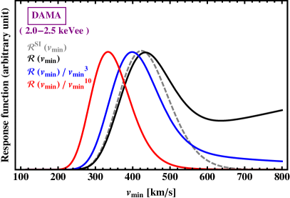
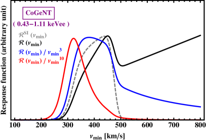
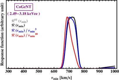
In Fig. 1 we illustrate the effect of various choices of on the response function for MDM for several energy bins and experiments: the first energy bin of DAMA/LIBRA [1], 2 to 2.5 keVee, the 7 to 9 keV CDMS-II used for the Si data [5] and the first, 0.43 to 1.11 keVee, and last, 2.49 to 3.18 keVee, of CoGeNT [2, 3]. We also include for the standard SI interaction (gray dashed line) for a comparison. The normalization of each curve is arbitrary. For , the MDM response function is divergent and goes like at large velocities, given the behavior of (see discussion at the beginning of Sec. 4). The divergent behavior is much more pronounced in the low-energy bins. The choice is already enough to regularize the divergent behavior, but still yields too large intervals. For growing values of , the peak of the response function, mostly in the low energy bins, shifts towards low velocities, due to the factor. This peak, when far from the interval where is non-negligible, is unreliable as it is due to the low energy tail of the detector energy resolution function , which determines the low velocity tail of (see Eq. (20)) and is never well known. We found the optimum value by trial an error and for MDM we find that is an adequate choice (see Fig. 1) to get a localized response function in space without relying on how the low energy tail of the energy resolution function is modeled. The choice of is dictated by the lowest energy bins, where the function is largest. Higher energy bins are less sensitive to the choice of .
Let us remark that this way of comparing data is not an inherent part to the halo independent method but only due to our choice of finding averages over measured energy bins to translate putative measurements of a DM signal. So far we have not found a better way of presenting the data, but more work is necessary to make progress in this respect.
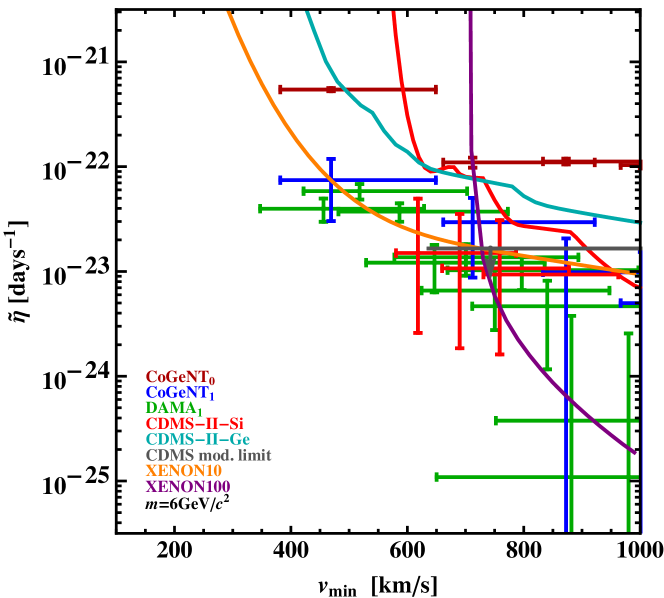
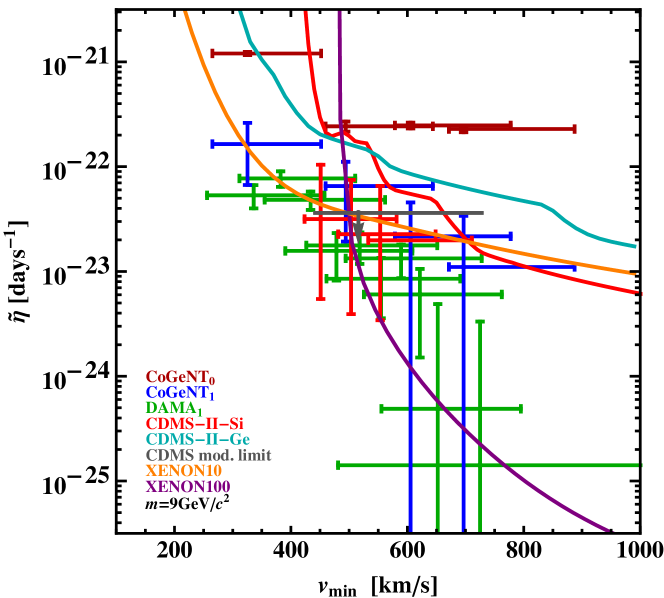
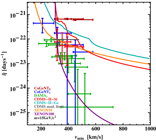
Figs. 2, 3 and 4 show the measurements and bounds on and for a WIMP with magnetic dipole interactions (MDM). To compute the position of the lines, no average is taken so that the bound corresponds to a limit on .
In both figures we include the DAMA modulation signal (green crosses), CoGeNT modulated (blue crosses) and unmodulated signal (plus an unknown flat background, dark red horizontal lines), CDMS-II-Si unmodulated rate signal (red crosses and limit line), CDMS-II-Ge unmodulated rate limit (light blue line) and modulation bound (dark grey horizontal line), XENON100 225 days limit (purple line) and XENON10 S2 only limit (orange line).
Figs. 2, 3 and 4 differ for the value of the DM mass, respectively GeV, GeV and GeV. We chose these masses motivated by previous studies on MDM as a potential explanation for the putative DM signal found by DAMA/LIBRA, CoGeNT and CRESST-II (see e.g. Ref. [48]). The measurements and limits for MDM move to larger values as the WIMP mass increases, as expected due to the relation between and the recoil energy. As shown in Fig. 2, for a WIMP of mass GeV the three CDMS-II-Si points are largely below the XENON10 and XENON100 upper limits, but they move progressively above them as increases to 9 GeV, see Fig. 3, and are almost entirely excluded by them for GeV in Fig. 4. The three CDMS-II-Si points overlap or are below the CoGeNT and DAMA/LIBRA measurements of the modulated part of , except for the lowest energy CoGeNT and DAMA points. Thus, interpreted as a measurement of the unmodulated rate, the three CDMS-II-Si data points seem largely incompatible with the modulation of the signal observed by CoGeNT and DAMA for MDM. For all three WIMP masses shown in the figures, the DAMA and CoGeNT modulation measurements seem compatible with each other, but the upper limits on the unmodulated part of the rate imposed by XENON10 and XENON100 reject the DAMA/LIBRA and CoGeNT modulation signal, except for the lowest energy bins, for MDM.
7 Conclusions
We have presented a way to generalize to any DM–target nucleus interaction the halo-independent method to compare direct dark matter results from different experiments, initially proposed in Ref [13] and used already in several subsequent papers [14, 15, 16, 17, 18, 19, 20]. The method avoids the complications brought about by astrophysical uncertainties that affect the interaction rate.
The main idea of this method is that the interaction rate at one particular recoil energy depends for any experiment on one and the same function of the minimum speed required for the incoming DM particle to cause a nuclear recoil with energy . The function depends only on the local characteristics of the dark halo of our galaxy. Thus, all rate measurements and bounds can be translated into measurements and bounds on the unique function . Before the present work, this method was applied to the standard spin-independent (SI) WIMP-nucleus interaction only, although it could easily be applied to the standard spin-dependent (SD) interaction as well. For both SI and SD interactions, the differential scattering cross section has a dependence on the speed of the DM particle. However, there are many other kinds of interactions with more general dependence on the DM particle velocity and on the nuclear recoil energy and for some of them the trivial extension of the SI method does not work. This is the case, for example when the cross section contains two different terms with different dependences on the DM particle speed . Then, when these terms are integrated over the velocity distribution to find the rate, instead of a unique function , each term has its own function of multiplied by its own detector dependent coefficient. It is thus impossible to translate a rate measurement or bound into only one of the two functions contributing to the rate.
In Eq. (26) we have presented a way to write the rate measured in a certain energy range (expressed in observed energy , not in actual recoil energy ) for any kind of interaction in terms of a unique function of , which we called , that depends on the local characteristics of the dark halo of our galaxy only convolved with a detector and DM candidate dependent response function in , . This response function is defined in Eq. (27), as the derivative of what we call the “integrated response function” defined in Eq. (20) or Eq. (21) in terms of the scattering cross section and detector characteristics (composition, energy resolution, efficiency cuts).
Since the function must be common to all experiments, we can map all the rate measurements and bounds obtained with different experiments into the plane, as in the case of SI interactions. We have then chosen a way to compare all data for magnetic dipole moment DM (MDM) by comparing weighted averages of the derived from experiments with a potential DM signal and upper bounds on derived from data which do not find a possible DM signal. The average is weighted by the response function and corresponds to the interval in which this weight function is significantly different from zero. However, we found that for a differential cross section with a general dependence on the DM velocity the width of the response function in Eq. (27) at large , which is dictated by the high speed behavior of the differential cross section, might even be infinite. For example, if goes as , with a positive integer, for large , then also goes as and goes as for large . Thus, if , the response function does not vanish for large . However, we can regularize the behavior of the response function at large by using for example the function with integer , instead of just . Since this new function is common to all experiments, we can use it to compare the data in space. The power cannot be chosen arbitrarily large, because large values of give a large weight to the low velocity tail of the function, and this tail depends on the low energy tail of the experimental energy resolution function in Eq. (20), which is never well known. Therefore too large values of make the procedure very sensitive to the way in which the tails of the function are modeled. For the particular example of interaction we present in this paper, magnetic dipole DM or MDM, we found that an optimal choice is . In the figures, rather than drawing the new averages and the limits , we prefer to draw and , so that a comparison can be easily made with the previous literature on the SI halo-independent method.
Let us remark that this way of comparing data is not an inherent part to the halo independent method but only due to our choice of finding averages over measured energy bins to translate putative measurements of a DM signal. So far we have not found a better way of presenting the data, but more work is necessary to make progress in this respect.
Acknowledgments
P.G. was supported in part by NSF grant PHY-1068111. E.D.N., G.G. and J.-H.H. were supported in part by DOE grant DE-FG02-13ER42022. J.-H.H. was also partially supported by Spanish Consolider-Ingenio MultiDark (CSD2009-00064).
Appendix A - Inelastic scattering
The DM particle may collide inelastically with the target nucleus [66], in which case the DM particle scatters to a different state with mass . Dark matter interacting inelastically via a magnetic dipole moment interaction [39, 46] would require a modification of some of the equations presented above, in particular the definitions of . Here we present the relevant equations for the inelastic case.
In inelastic scattering, the minimum velocity the DM must have to impart a nuclear recoil energy depends on the mass splitting ,
| (42) |
where can be either positive (endothermic scattering [66]) or negative (exothermic [67]) ( for elastic scattering). Inverting this equation implies the existence of both a maximum and a minimum recoil energy for a fixed DM velocity : , with
| (43) |
The event rate in a detected energy interval is (as in Eq. (4))
| (44) |
Changing the order of the integrations in and in Eq. (44), we have
| (45) |
where is the minimum value can take, for and for . In compact form, Eq. (45) reads
| (46) |
where as in Eq. (19)
| (47) |
and
| (48) |
We will deal in detail with the halo independent comparison of direct detection data for dark matter with magnetic dipole interactions (MDM) scattering inelastically [39, 46] elsewhere.
Appendix B - Rate in terms of partial moments
In this appendix we derive Eqs. (29) and (31). Define, as in Eq. (28),
| (49) | ||||
| (50) |
Then
| (51) |
Repeatedly integrating by parts Eq. (26) gives
| (52) |
In deriving this result, all boundary terms vanish because we have assumed that the response function and all of its derivatives vanish at , since is below the threshold of any experiment.
References
- [1] R. Bernabei et al. [DAMA and LIBRA Collaborations], “New results from DAMA/LIBRA,” Eur. Phys. J. C 67 (2010) 39 [arXiv:1002.1028 [astro-ph.GA]].
- [2] C. E. Aalseth et al. [CoGeNT Collaboration], “Results from a Search for Light-Mass Dark Matter with a P-type Point Contact Germanium Detector,” Phys. Rev. Lett. 106 (2011) 131301 [arXiv:1002.4703 [astro-ph.CO]].
- [3] C. E. Aalseth, P. S. Barbeau, J. Colaresi, J. I. Collar, J. Diaz Leon, J. E. Fast, N. Fields and T. W. Hossbach et al., “Search for an Annual Modulation in a P-type Point Contact Germanium Dark Matter Detector,” Phys. Rev. Lett. 107 (2011) 141301 [arXiv:1106.0650 [astro-ph.CO]].
- [4] G. Angloher, M. Bauer, I. Bavykina, A. Bento, C. Bucci, C. Ciemniak, G. Deuter and F. von Feilitzsch et al., “Results from 730 kg days of the CRESST-II Dark Matter Search,” Eur. Phys. J. C 72 (2012) 1971 [arXiv:1109.0702 [astro-ph.CO]].
- [5] R. Agnese et al. [CDMS Collaboration], “Dark Matter Search Results Using the Silicon Detectors of CDMS II,” [arXiv:1304.4279 [hep-ex]].
- [6] J. Angle et al. [XENON10 Collaboration], “A search for light dark matter in XENON10 data,” Phys. Rev. Lett. 107 (2011) 051301 [arXiv:1104.3088 [astro-ph.CO]].
- [7] E. Aprile et al. [XENON100 Collaboration], “Dark Matter Results from 100 Live Days of XENON100 Data,” Phys. Rev. Lett. 107 (2011) 131302 [arXiv:1104.2549 [astro-ph.CO]].
- [8] E. Aprile et al. [XENON100 Collaboration], “Dark Matter Results from 225 Live Days of XENON100 Data,” Phys. Rev. Lett. 109 (2012) 181301 [arXiv:1207.5988 [astro-ph.CO]].
- [9] M. Felizardo, T. A. Girard, T. Morlat, A. C. Fernandes, A. R. Ramos, J. G. Marques, A. Kling and J. Puibasset et al., “Final Analysis and Results of the Phase II SIMPLE Dark Matter Search,” Phys. Rev. Lett. 108 (2012) 201302 [arXiv:1106.3014 [astro-ph.CO]].
- [10] Z. Ahmed et al. [CDMS-II Collaboration], “Results from a Low-Energy Analysis of the CDMS II Germanium Data,” Phys. Rev. Lett. 106 (2011) 131302 [arXiv:1011.2482 [astro-ph.CO]].
- [11] Z. Ahmed et al. [CDMS Collaboration], “Search for annual modulation in low-energy CDMS-II data,” arXiv:1203.1309 [astro-ph.CO].
- [12] R. Agnese et al. [CDMS Collaboration], “Silicon Detector Results from the First Five-Tower Run of CDMS II,” [arXiv:1304.3706 [astro-ph.CO]].
- [13] P. J. Fox, J. Liu and N. Weiner, “Integrating Out Astrophysical Uncertainties,” Phys. Rev. D 83 (2011) 103514 [arXiv:1011.1915 [hep-ph]].
- [14] M. T. Frandsen, F. Kahlhoefer, C. McCabe, S. Sarkar and K. Schmidt-Hoberg, “Resolving astrophysical uncertainties in dark matter direct detection,” JCAP 1201 (2012) 024 [arXiv:1111.0292 [hep-ph]].
- [15] P. Gondolo and G. B. Gelmini, “Halo independent comparison of direct dark matter detection data,” JCAP 1212 (2012) 015 [arXiv:1202.6359 [hep-ph]].
- [16] M. T. Frandsen, F. Kahlhoefer, C. McCabe, S. Sarkar and K. Schmidt-Hoberg, “The unbearable lightness of being: CDMS versus XENON,” arXiv:1304.6066 [hep-ph].
- [17] E. Del Nobile, G. B. Gelmini, P. Gondolo and J. -H. Huh, “Halo-independent analysis of direct detection data for light WIMPs,” arXiv:1304.6183 [hep-ph].
- [18] J. Herrero-Garcia, T. Schwetz and J. Zupan, “On the annual modulation signal in dark matter direct detection,” JCAP 1203 (2012) 005 [arXiv:1112.1627 [hep-ph]].
- [19] J. Herrero-Garcia, T. Schwetz and J. Zupan, “Astrophysics independent bounds on the annual modulation of dark matter signals,” Phys. Rev. Lett. 109 (2012) 141301 [arXiv:1205.0134 [hep-ph]].
- [20] N. Bozorgnia, J. Herrero-Garcia, T. Schwetz and J. Zupan, “Halo-independent methods for inelastic dark matter scattering,” arXiv:1305.3575 [hep-ph].
- [21] J. Bagnasco, M. Dine and S. D. Thomas, “Detecting technibaryon dark matter,” Phys. Lett. B 320 (1994) 99 [hep-ph/9310290].
- [22] A. Kurylov and M. Kamionkowski, “Generalized analysis of weakly interacting massive particle searches,” Phys. Rev. D 69 (2004) 063503 [hep-ph/0307185].
- [23] B. A. Dobrescu and I. Mocioiu, “Spin-dependent macroscopic forces from new particle exchange,” JHEP 0611 (2006) 005 [hep-ph/0605342].
- [24] J. Fan, M. Reece and L. -T. Wang, “Non-relativistic effective theory of dark matter direct detection,” JCAP 1011 (2010) 042 [arXiv:1008.1591 [hep-ph]].
- [25] A. L. Fitzpatrick, W. Haxton, E. Katz, N. Lubbers and Y. Xu, “The Effective Field Theory of Dark Matter Direct Detection,” JCAP 1302 (2013) 004 [arXiv:1203.3542 [hep-ph]].
- [26] M. Beltran, D. Hooper, E. W. Kolb and Z. C. Krusberg, “Deducing the nature of dark matter from direct and indirect detection experiments in the absence of collider signatures of new physics,” Phys. Rev. D 80 (2009) 043509 [arXiv:0808.3384 [hep-ph]].
- [27] S. Chang, A. Pierce and N. Weiner, “Momentum Dependent Dark Matter Scattering,” JCAP 1001 (2010) 006 [arXiv:0908.3192 [hep-ph]].
- [28] J. -M. Zheng, Z. -H. Yu, J. -W. Shao, X. -J. Bi, Z. Li and H. -H. Zhang, “Constraining the interaction strength between dark matter and visible matter: I. fermionic dark matter,” Nucl. Phys. B 854 (2012) 350 [arXiv:1012.2022 [hep-ph]].
- [29] Z. -H. Yu, J. -M. Zheng, X. -J. Bi, Z. Li, D. -X. Yao and H. -H. Zhang, “Constraining the interaction strength between dark matter and visible matter: II. scalar, vector and spin-3/2 dark matter,” Nucl. Phys. B 860 (2012) 115 [arXiv:1112.6052 [hep-ph]].
- [30] K. Cheung, P. -Y. Tseng, Y. -L. S. Tsai and T. -C. Yuan, “Global Constraints on Effective Dark Matter Interactions: Relic Density, Direct Detection, Indirect Detection, and Collider,” JCAP 1205 (2012) 001 [arXiv:1201.3402 [hep-ph]].
- [31] J. March-Russell, J. Unwin and S. M. West, “Closing in on Asymmetric Dark Matter I: Model independent limits for interactions with quarks,” JHEP 1208 (2012) 029 [arXiv:1203.4854 [hep-ph]].
- [32] R. Ding and Y. Liao, “Spin 3/2 Particle as a Dark Matter Candidate: an Effective Field Theory Approach,” JHEP 1204 (2012) 054 [arXiv:1201.0506 [hep-ph]].
- [33] M. Pospelov and T. ter Veldhuis, “Direct and indirect limits on the electromagnetic form-factors of WIMPs,” Phys. Lett. B 480 (2000) 181 [hep-ph/0003010].
- [34] A. L. Fitzpatrick and K. M. Zurek, “Dark Moments and the DAMA-CoGeNT Puzzle,” Phys. Rev. D 82 (2010) 075004 [arXiv:1007.5325 [hep-ph]].
- [35] H. An, S. -L. Chen, R. N. Mohapatra, S. Nussinov and Y. Zhang, “Energy Dependence of Direct Detection Cross Section for Asymmetric Mirror Dark Matter,” Phys. Rev. D 82 (2010) 023533 [arXiv:1004.3296 [hep-ph]].
- [36] S. D. McDermott, H. -B. Yu and K. M. Zurek, “Turning off the Lights: How Dark is Dark Matter?,” Phys. Rev. D 83 (2011) 063509 [arXiv:1011.2907 [hep-ph]].
- [37] K. Sigurdson, M. Doran, A. Kurylov, R. R. Caldwell and M. Kamionkowski, “Dark-matter electric and magnetic dipole moments,” Phys. Rev. D 70 (2004) 083501 [Erratum-ibid. D 73 (2006) 089903] [astro-ph/0406355].
- [38] V. Barger, W. -Y. Keung and D. Marfatia, “Electromagnetic properties of dark matter: Dipole moments and charge form factor,” Phys. Lett. B 696 (2011) 74 [arXiv:1007.4345 [hep-ph]].
- [39] S. Chang, N. Weiner and I. Yavin, “Magnetic Inelastic Dark Matter,” Phys. Rev. D 82 (2010) 125011 [arXiv:1007.4200 [hep-ph]].
- [40] W. S. Cho, J. -H. Huh, I. -W. Kim, J. E. Kim and B. Kyae, “Constraining WIMP magnetic moment from CDMS II experiment,” Phys. Lett. B 687 (2010) 6 [Erratum-ibid. B 694 (2011) 496] [arXiv:1001.0579 [hep-ph]].
- [41] J. H. Heo, “Minimal Dirac Fermionic Dark Matter with Nonzero Magnetic Dipole Moment,” Phys. Lett. B 693 (2010) 255 [arXiv:0901.3815 [hep-ph]].
- [42] S. Gardner, “Shedding Light on Dark Matter: A Faraday Rotation Experiment to Limit a Dark Magnetic Moment,” Phys. Rev. D 79 (2009) 055007 [arXiv:0811.0967 [hep-ph]].
- [43] E. Masso, S. Mohanty and S. Rao, “Dipolar Dark Matter,” Phys. Rev. D 80 (2009) 036009 [arXiv:0906.1979 [hep-ph]].
- [44] T. Banks, J. -F. Fortin and S. Thomas, “Direct Detection of Dark Matter Electromagnetic Dipole Moments,” arXiv:1007.5515 [hep-ph].
- [45] J. -F. Fortin and T. M. P. Tait, “Collider Constraints on Dipole-Interacting Dark Matter,” Phys. Rev. D 85 (2012) 063506 [arXiv:1103.3289 [hep-ph]].
- [46] K. Kumar, A. Menon and T. M. P. Tait, “Magnetic Fluffy Dark Matter,” JHEP 1202 (2012) 131 [arXiv:1111.2336 [hep-ph]].
- [47] V. Barger, W. -Y. Keung, D. Marfatia and P. -Y. Tseng, “Dipole Moment Dark Matter at the LHC,” Phys. Lett. B 717 (2012) 219 [arXiv:1206.0640 [hep-ph]].
- [48] E. Del Nobile, C. Kouvaris, P. Panci, F. Sannino and J. Virkajarvi, “Light Magnetic Dark Matter in Direct Detection Searches,” JCAP 1208 (2012) 010 [arXiv:1203.6652 [hep-ph]].
- [49] J. M. Cline, Z. Liu and W. Xue, “Millicharged Atomic Dark Matter,” Phys. Rev. D 85 (2012) 101302 [arXiv:1201.4858 [hep-ph]].
- [50] N. Weiner and I. Yavin, “How Dark Are Majorana WIMPs? Signals from MiDM and Rayleigh Dark Matter,” Phys. Rev. D 86 (2012) 075021 [arXiv:1206.2910 [hep-ph]].
- [51] S. Tulin, H. -B. Yu and K. M. Zurek, “Three Exceptions for Thermal Dark Matter with Enhanced Annihilation to ,” Phys. Rev. D 87 (2013) 036011 [arXiv:1208.0009 [hep-ph]].
- [52] J. M. Cline, A. R. Frey and G. D. Moore, “Composite magnetic dark matter and the 130 GeV line,” Phys. Rev. D 86 (2012) 115013 [arXiv:1208.2685 [hep-ph]].
- [53] M. Pospelov and A. Ritz, “Resonant scattering and recombination of pseudo-degenerate WIMPs,” Phys. Rev. D 78 (2008) 055003 [arXiv:0803.2251 [hep-ph]].
- [54] Y. Bai and P. J. Fox, “Resonant Dark Matter,” JHEP 0911 (2009) 052 [arXiv:0909.2900 [hep-ph]].
- [55] B. Feldstein, A. L. Fitzpatrick and E. Katz, “Form Factor Dark Matter,” JCAP 1001 (2010) 020 [arXiv:0908.2991 [hep-ph]].
- [56] C. M. Ho and R. J. Scherrer, “Anapole Dark Matter,” Phys. Lett. B 722 (2013) 341 [arXiv:1211.0503 [hep-ph]].
- [57] R. H. Helm, “Inelastic and Elastic Scattering of 187-Mev Electrons from Selected Even-Even Nuclei,” Phys. Rev. 104 (1956) 1466.
- [58] T. W. Donnelly and I. Sick, “Elastic Magnetic Electron Scattering From Nuclei,” Rev. Mod. Phys. 56 (1984) 461.
- [59] N. Bozorgnia, G. B. Gelmini and P. Gondolo, “Channeling in direct dark matter detection I: channeling fraction in NaI (Tl) crystals,” JCAP 1011 (2010) 019 [arXiv:1006.3110 [astro-ph.CO]].
- [60] J. I. Collar, “Quenching and Channeling of Nuclear Recoils in NaI[Tl]: Implications for Dark Matter Searches,” arXiv:1302.0796 [physics.ins-det].
- [61] J. Collar, private communication.
- [62] C. E. Aalseth et al. [CoGeNT Collaboration], “CoGeNT: A Search for Low-Mass Dark Matter using p-type Point Contact Germanium Detectors,” Physical Review D 88, 012002 (2013) [arXiv:1208.5737 [astro-ph.CO]].
- [63] S. Yellin, “Finding an upper limit in the presence of unknown background,” Phys. Rev. D 66 (2002) 032005 [physics/0203002].
- [64] Z. Ahmed et al. [CDMS Collaboration], “Analysis of the low-energy electron-recoil spectrum of the CDMS experiment,” Phys. Rev. D 81 (2010) 042002 [arXiv:0907.1438 [astro-ph.GA]].
- [65] E. Aprile et al. [XENON100 Collaboration], “Likelihood Approach to the First Dark Matter Results from XENON100,” Phys. Rev. D 84 (2011) 052003 [arXiv:1103.0303 [hep-ex]].
- [66] D. Tucker-Smith and N. Weiner, “Inelastic dark matter,” Phys. Rev. D 64 (2001) 043502 [hep-ph/0101138].
- [67] P. W. Graham, R. Harnik, S. Rajendran and P. Saraswat, “Exothermic Dark Matter,” Phys. Rev. D 82 (2010) 063512 [arXiv:1004.0937 [hep-ph]].