Modeling X-ray binary evolution in normal galaxies: Insights from SINGS

Abstract

We present the largest-scale comparison to date between observed extragalactic X-ray binary (XRB) populations and theoretical models of their production. We construct observational X-ray luminosity functions (oXLFs) using Chandra observations of 12 late-type galaxies from the Spitzer Infrared Nearby Galaxy Survey (SINGS). For each galaxy, we obtain theoretical XLFs (tXLFs) by combining XRB synthetic models, constructed with the population synthesis code StarTrack, with observational star formation histories (SFHs). We identify highest-likelihood models both for individual galaxies and globally, averaged over the full galaxy sample. Individual tXLFs successfully reproduce about half of oXLFs, but for some galaxies we are unable to find underlying source populations, indicating that galaxy SFHs and metallicities are not well matched and/or XRB modeling requires calibration on larger observational samples. Given these limitations, we find that best models are consistent with a product of common envelope ejection efficiency and central donor concentration $\simeq 0.1$, and a 50% uniform – 50% “twins” initial mass-ratio distribution. We present and discuss constituent subpopulations of tXLFs according to donor, accretor and stellar population characteristics. The galaxy-wide X-ray luminosity due to low-mass and high-mass XRBs, estimated via our best global model tXLF, follows the general trend expected from the $L_{X}$ - star formation rate and $L_{X}$ - stellar mass relations of Lehmer et al. (2010). Our best models are also in agreement with modeling of the evolution both of XRBs over cosmic time and of the galaxy X-ray luminosity with redshift.

1. Introduction

Binary stars constitute a substantial fraction of stellar populations (SPs). In galactic fields and low density agglomerations such as open clusters between $\sim 40$% and $\sim 75$% of stars are binaries (Duquennoy & Mayor, 1991; Fischer & Marcy, 1992; Fan et al., 1996; Raghavan et al., 2010; Sana et al., 2012). In fact, stellar binarity may well be a universal characteristic of stellar evolution, since many single stars may either have been through a binary phase, only to be ejected later, or be the result of a binary merger (Sana et al., 2012). Compared to single stars, binary stars are hosts to a range of additional processes (mass and angular momentum transfer, wind accretion, Roche-lobe overflow, common envelope ejection etc.), making them ideal astrophysical laboratories for a whole range of physics not represented among single stars. Some of the most interesting processes that can be probed are associated with accretion onto primaries that are compact objects (neutron stars and black holes). Due to the extreme energies involved, such cases are observationally identified as X-ray binaries (XRBs).

There have been many observational studies of XRB populations in external galaxies. Earlier work with the Einstein satellite showed that the X-ray emission is dominated by XRBs with low-mass (LMXBs) or high-mass donors (HMXBs) in early and late-type galaxies, respectively (Kim et al., 1992). Using Chandra’s sub-arcsecond resolution, this result has now been established for individually detected XRBs in nearby galaxies (e.g. Kong et al., 2002; Soria & Kong, 2002; Trudolyubov et al., 2002; Sivakoff et al., 2003; Kim & Fabbiano, 2003; Gilfanov et al., 2004; Gilfanov, 2004; Kim & Fabbiano, 2004; Zhang et al., 2012; Binder et al., 2012, 2013, see also Fabbiano (2006) and references therein). Due to the longer evolutionary timescales of LMXBs, their integrated X-ray emission is an indicator of a galaxy’s total stellar mass (Gilfanov, 2004; Bogdán & Gilfanov, 2010; Zhang et al., 2011; Boroson et al., 2011). In contrast, relatively short-lived HMXBs probe a galaxy’s star formation rate ((SFR), Grimm et al., 2003; Ranalli et al., 2003; Gilfanov et al., 2004; Persic & Rephaeli, 2007; Shtykovskiy & Gilfanov, 2007; Lehmer et al., 2010; Mineo et al., 2012). These observations have also established a break in the XLF of LMXBs at low luminosities ($L_{X}\sim 10^{37}$ erg s^-1, Gilfanov, 2004; Revnivtsev et al., 2008, 2011) both in the Milky Way and in external galaxies.

In the past, semi-analytical theoretical models have been introduced for the study of XRB populations. White & Ghosh (1998) and Ghosh & White (2001), assumed a time-dependent SFR and a simple rate model to study the evolution of an arbitrary XRB population. These models predicted that the time required for binaries to reach the X-ray phase leads to a significant time delay between a star-formation episode and the production of X-ray emission from X-ray binaries from the population. Wu (2001) created a simple birth-death model, in which the lifetimes of the binaries are inversely proportional to their X-ray luminosity, and calculated the XLFs of spiral galaxies. His models reproduce some features, such as the luminosity break in the observed XLFs of spiral galaxies. Piro & Bildsten (2002) argued that the majority of LMXBs in the field of elliptical galaxies have red giant donors feeding a thermally unstable disk and stay in this transient phase for at least 75% of their life. Most recently, in a series of papers, Bhadkamkar & Ghosh (2012, 2013a, 2013b) started from standard distributions of the parameters of those primordial binaries which are the progenitors of XRBs, and followed the transformation of these distributions with the aid of a Jacobian formalism as the binaries progress through different evolutionary phases. Following this methodology, they were able to derive estimates for the XLF and other population statistical properties, for both HMXBs and LMXBs.

Binary population synthesis (PS) modeling codes can provide a unique tool to understand the physical properties of this important population in a statistical sense. Lipunov et al. (1996) used for the first time a PS code to investigate the evolution of XRBs in the central part of the Milky Way over the course of 10 My (see Lipunov et al., 2009, for a description of their code “Scenario Machine”). A number of other codes have been developed mostly within the last decade or so (Hurley et al., 2002; Kiel & Hurley, 2006; Belczynski et al., 2008). These codes have been used by several authors to carry out a variety of investigations, including the study of double compact object mergers (e.g. Belczynski et al., 2002), the formation of ultrashort XRBs (e.g. Belczynski et al., 2004), the numbers and spatial distributions of XRBs in star clusters (e.g. Sepinsky et al., 2005), the evolution of XRBs in a brief star-formation episode as a model of starburst systems (Eracleous et al., 2006), the formation of binary millisecond pulsars (e.g. Pfahl et al., 2003; Hurley et al., 2010), binary fractions in globular clusters (e.g. Ivanova et al., 2005; Hurley et al., 2007), and numbers and birthrates of symbiotic XRBs in the Galaxy (e.g. Lü et al., 2012).

Physically motivated PS modeling and detailed comparisons of XLF characteristics can be used to understand how these observations are linked to the formation and evolution of XRB populations in galaxies. This type of work was pioneered by Belczynski et al. (2004) who compared a theoretical X-ray luminosity function (tXLF) with observational X-ray luminosity functions (oXLFs) for XRBs in the dwarf irregular galaxy NGC 1569 obtained with Chandra. Linden et al. (2009, 2010) studied the XLF for HMXBs and Be XRBs in the SMC. Fragos et al. (2008, 2009) modeled the XLFs in the two elliptical galaxies NGC 3379 and NGC 4278, and investigated the contributions from subpopulations of LMXBs. Zuo & Li (2011) used the PS code of Hurley et al. (2002) to investigate the X-ray-evolution of late-type galaxies over $\sim 14$ Gy of cosmic time.

To carry out this type of work, it is necessary to combine PS models with star formation history (SFH) information for specific galaxies. For their elliptical galaxies Fragos et al. (2008, hereafter F08) assumed an initial $\delta$-function star formation episode. For later type galaxies SFH can be obtained via spectral energy distribution (SED) modeling, which requires multiwavelength information for a given galaxy.

In this paper we use a sample of 12 nearby galaxies from the Spitzer Infrared Nearby Galaxy Survey (SINGS) covering a range in star forming properties to extend binary PS modeling to later type systems. We construct oXLFs for their off-nuclear point source XRB populations and tXLFs by combining population synthesis modeling results, obtained by means of the PS code StarTrack, and star formation histories from the literature. This allows us to compare the two sets of XRB XLFs and investigate the range of acceptable values for XRB formation and evolution parameters.

This paper is part of a larger effort to understand the formation and evolution of extragalactic XRBs by means of the most advanced PS modeling to date. Other papers in the series include Fragos et al. (2013, hereafter F13) and Tremmel et al. (2013, accepted, astroph/1210.7185, hereafter T13). F13 study the evolution of the global XRB population with redshift by using the Millennium-II simulation as initial conditions. They accurately reproduce local group HMXB and LMXB luminosity scaling relations with SFR and $M_{*}$ (Lehmer et al., 2010; Mineo et al., 2012), respectively. T13 use the same initial conditions to explain observational XLFs for the integrated XRB emission from entire galaxies (Tzanavaris & Georgantopoulos, 2008) and make predictions for higher redshifts. In this paper we apply the same grid of PS models, combining it with SFH information for nearby galaxies (Noll et al., 2009).

The structure of the paper is as follows: In Section 2 we present the observational sample and the construction of oXLFs. Section 3 discusses the calculation of tXLFs. Section 4 presents likelihood functions for establishing best PS models. Results are presented and discussed in Section 5. Section 6 gives a summary and discusses future prospects.

2. Observational Sample and XLFs

We use galaxies selected from the Spitzer Infrared Nearby Galaxy Survey (SINGS, Kennicutt et al., 2003). This survey was designed to be a diverse sample of intrinsic galaxy properties with multiwavelength data ranging from the ultraviolet to the far infrared. As part of a large Chandra program (XSINGS, Jenkins et al., 2010), the Advanced CCD Imaging Spectrometer (ACIS) was used to extend the survey’s wavelength coverage to the X-ray regime. Details regarding the sample selection, X-ray observations, source detection and characterization will be presented in a forthcoming publication (Jenkins et al., in prep.) Briefly, basic X-ray data reduction was carried out using standard Chandra X-ray Center tools. Point source detection was performed in the soft (0.3-2.0 keV), hard (2.0-10.0 keV) and full (0.3-10.0 kev) band with CIAO wavdetect to construct a candidate source list. The final list was produced by using the software acis extract (ae, Broos et al., 2010) to perform aperture photometry and produce a catalog of point sources with associated fluxes and luminosities for each galaxy.

We use a sub-sample of 12 SINGS galaxies that have SFHs from spectral energy distribution fitting with the code CIGALE (Noll et al., 2009). Galaxies are also selected to have at least 15 detected, non-nuclear, X-ray point sources as a prerequisite for the production of meaningful XRB XLFs. Details of the galaxy sample are given in Table Modeling X-ray binary evolution in normal galaxies: Insights from SINGS. Spitzer-infrared and Chandra-X-ray galaxy images are shown in Fig. 1. To illustrate the properties of our sample relative to the rest of the SINGS galaxies, in Fig. 2 we show both a color-magnitude diagram and a plot of star formation rate vs. stellar mass for the full SINGS sample, highlighting our galaxies. In both plots, galaxies are separated into three broad morphological categories, namely E/S0 (shown in red), Sa-Sbc (magenta), and Sc-Im (blue). Compared to the rest of the SINGS galaxies, our systems have intermediate to high SFR and $M_{\ast}$, and intermediate to red colors.

At low point source luminosities incompleteness effects arise, compromising the construction of unbiased XLFs. These can be mitigated either by limiting observational XLFs to the luminosity range in which incompleteness is not significant or by performing incompleteness corrections. The second approach is preferable since it allows the construction of XLFs covering a wider dynamic range in X-ray luminosity. We use the method of Zezas et al. (2007, see also ()) to create simulated X-ray source catalogs, calculate the source detection probabilities and obtain incompleteness corrections as a function of source and background intensity (in counts) and off-axis angle for X-ray detected sources. Note that this detection probability is otherwise independent of other source characteristics such as detection band and intrinsic source spectrum.

oXLFs are shown in Fig. 3 by the blue curves before (dotted) and after (solid) completeness correction. In practice, we find that completeness corrections are small and do not change the models that are associated with the highest-likelihood tXLF for a given galaxy. Specifically, a quality check on our best populated galaxy NGC 1291, for which we apply both methods, shows that our conclusions do not change. We note that the highest-likelihood tXLF is also shown in Fig. 3 (in red and dark grey; see Sec. 4 for details).

3. Population Synthesis Modeling

3.1. StarTrack

The main tool we use to perform our PS simulations is StarTrack, a state-of-the-art PS code that has been tested and calibrated using detailed mass transfer star calculations and observations of binary populations. StarTrack has been applied to numerous interpretation studies of X-ray and radio pulsar binary populations, as well as $\gamma$-ray bursts and binary black holes in the context of gravitational-wave sources (see detailed description in Belczynski et al., 2008, and references therein). In summary the code incorporates all the important physical processes of binary evolution:

(i) The evolution of single stars and non-interacting binary components from zero-age main sequence to remnant formation is followed with the use of high-quality analytic formulae (Hurley et al., 2000). Various wind mass loss rates dependent on stellar evolutionary stage are incorporated and their effect on stellar evolution is taken into account.

(ii) Changes in all the orbital properties are tracked. Through numerical integration of four differential equations, the evolution of orbital separation, eccentricity and component spins is tracked; these depend on tidal interactions as well as angular momentum losses associated with magnetic braking, gravitational radiation and stellar wind mass losses.

(iii) All types of mass-transfer phases are calculated: Stable, driven by nuclear evolution or angular momentum loss, and thermally or dynamically unstable.

(iv) Supernova explosions are treated accounting for mass loss and asymmetries with natal kicks to neutron stars and black holes at birth; systemic velocities for all binaries are calculated.

(v) The calculation of mass transfer rates in binaries with accreting neutron stars and black holes (driven by stellar winds or Roche-lobe overflow) has been calibrated against detailed mass transfer sequences, and X-ray luminosities are calculated by incorporating appropriate band-pass corrections and spectral models.

This paper uses results that are based on a recent major revision of the StarTrack code that includes updated stellar wind prescriptions and their re-calibrated dependence on metallicity (Belczynski et al., 2010). Two newer updates have not been taken into account, as our simulations were complete before these updates had been implemented. For reference, these are (1) a revised neutron star and black hole mass spectrum, leading to fully consistent supernova simulations (Belczynski et al., 2012; Fryer et al., 2012); and (2) a more physical treatment of donor stars in common envelopes via actual $\lambda$ values (Dominik et al., 2012), where $\lambda$ is a measure of the donor’s central concentration and the envelope binding energy.

Table 1 lists the full set of input parameters used in our PS modeling. We construct a large PS model grid by using a range of values for these parameters as indicated in the table. For detailed discussion of how each parameter affects the overall XRB population, we refer the reader to F13 (Section 5.1 and Fig. 6) and T13 (Section 4.3 and Fig. 7).

The input parameters fall into two categories. First, parameters that mostly characterize initial properties of the population, such as initial mass function (IMF), initial binary mass ratio ($q$), and distribution of initial orbital separations. For these parameters we usually have information from observational surveys of binary stars, constraining the range of values used. The second category comprises parameters that are associated with physical processes that are poorly understood, such as the efficiency, $\alpha_{\rm CE}$, of converting orbital into thermal energy that will be used to expel the donor’s envelope during a common envelope (CE) phase. In this work the related parameter varied is $\lambda\alpha_{\rm CE}$, which is the product of this efficiency and the donor central concentration, $\lambda$.

The complete grid of 288 PS models is the same as that used by F13 and T13. To construct this grid, we vary all parameters known from earlier studies to affect XRB evolution and formation of compact objects (Belczynski et al., 2007; Fragos et al., 2008, 2009; Linden et al., 2009; Belczynski et al., 2010; Fragos et al., 2010). Specifically we use:

• Four $\lambda\alpha_{\rm CE}$ values (0.1, 0.2, 0.3, 0.5);

• Three stellar wind strengths, $\eta_{\rm wind}$ (0.25, 1.0, 2.0). This parameter is used to multiply the stellar wind prescription of Belczynski et al. (2010);

• The distribution of natal kicks for BHs formed through direct collapse (no kicks or 10% of the Hobbs et al. (2005) distribution for NSs);

• A CE-HG flag for systems with a donor in the Hertzsprung gap, either allowing all possible common envelope events or always imposing a merger (Belczynski et al., 2007);

• Three distributions of binary initial mass ratios, $q\equiv M_{\rm secondary}/M_{\rm primary}$. This distribution specifies the mass of the secondary, whereas the mass of the primary is governed by the IMF. For our full model grid, we use a uniform (flat) distribution, $q=0\rightarrow 1$, a twins distribution, $q=0.9\rightarrow 1$, and a mixed distribution, 50% uniform and 50% twins. However, in this paper we do not use the 96 twin $q$ models $97-192$, as F13 have already clearly shown that these are very inadequate in reproducing observed XRB populations, as they prevent the production of LMXBs altogether. This limits the models used in this paper to those in the ranges $1-96$ and $193-288$, i.e. 192 models in total.

In addition, for each of the 288 models in our full grid, we also use nine metallicities, keeping all other parameters same. In this paper we only consider solar metallicity models, as the best estimates of Moustakas et al. (2010) using two different methods appear to straddle solar metallicity for all SINGS galaxies in our study. The best fit SEDs that we convolve with StarTrack models to construct tXLFs for individual galaxies also assume solar metallicities (Noll et al., 2009).

Each model follows the evolution of $5.12\times 10^{6}$ stars over 14 Gyr. Since we are only using models $1-96$, corresponding to a uniform $q$ distribution, and models $193-288$, corresponding to a 50% – 50% mixed $q$ distribution, in relevant figures we indicate these model ranges for clarity. For reference, the full list of 288 models and associated parameters can be found in Table 4 of F13.

3.2. Theoretical X-ray luminosities

Since our goal is to construct XRB XLFs, we need to identify all binaries in our simulations that become XRBs and register their X-ray luminosities as a function of time. XRBs are mass-transferring binary stellar systems with a compact object accretor, either a black hole (BH) or a neutron star (NS). Systems with donors less massive than 3$M_{\odot}$ are labeled LMXBs, and vice versa for HMXBs. LMXBs are always Roche lobe overflowing (RLOF) systems, while HMXBs are usually wind-fed, but can also exhibit RLOF behavior. According to whether they undergo thermal disk instability or not, RLOF systems can be either transient or persistent, while wind-fed systems are always persistent.

We follow the methodology described in F08 and Fragos et al. (2009) to identify all model XRB sources and keep track of properties essential for estimating their X-ray luminosity, $L_{X}$, as a function of time. These properties include the mass-transfer rate, $\dot{M}$, as well as the mass and radius of the accretor, $M_{a}$ and $R_{a}$, respectively. We also identify BH or NS accretors, transient or persistent sources, evolutionary stages of donors and donor masses.

3.2.1 RLOF systems

For persistent systems, $L_{X}$ is estimated as

$$L_{X}={\rm min}\left(fL_{\rm Edd},\eta_{\rm bol}\epsilon\frac{GM_{a}\dot{M}}{R_{a}}\right)\ ,$$ (1)

with $f$ equal to unity. The value of $R_{a}$ is 10 km for a NS and 3 Schwarzschild radii for a BH, $\epsilon$ gives a conversion efficiency of gravitational binding energy to radiation associated with accretion onto a NS (surface accretion, $\epsilon=1.0$) or BH (disk accretion, $\epsilon=0.5$), and $\eta_{\rm bol}$ is a factor that converts the bolometric luminosity to $L_{X,{\rm 0.3-10.0keV}}$, the X-ray luminosity in the full Chandra energy band, consistent with our observations. We use results from the literature to tabulate the best available estimates of this factor and its $1\sigma$ uncertainty for neutron star and black hole accretors in “low-hard” and “high-soft” state systems (see F13 for a detailed discussion and references). Since we are interested in combining our PS models with galaxy star formation histories, we define lookback-time windows, $\delta t_{\rm lb}$, in which we evaluate the total stellar mass produced in the galaxies (see Sec. 3.3). In the StarTrack simulations each model source is associated with its own time-step window, $\delta t_{\rm step}$, which we use to calculate the fractional time, $\delta N$, that a source is on in a given galaxy lookback time interval, i.e.

$$\delta N\equiv\delta t_{\rm step}/\delta t_{\rm lb}\ .$$ (2)

For transient systems we follow the prescription of F08, calculating the outburst X-ray luminosity depending on the accretor type, either BH or NS, via

$$L_{\rm X}=\eta_{\rm bol}\epsilon\times\Bigg{\{}\begin{array}[]{l}\min{\left(f_{\rm BH}\times L_{\rm Edd},f_{\rm BH}\times L_{\rm Edd}\left[\frac{P}{10\rm h}\right]\right)},\rm{for\ BH}\\ \\ \min{\left(f_{\rm NS}\times L_{\rm Edd},\frac{GM_{a}\dot{M}_{\rm crit}^{2}}{R_{a}\dot{M}_{d}}\right)},\rm{for\ NS}\\ \end{array}$$ (3)

Here $f_{\rm BH},f_{\rm NS}$ are factors setting an upper limit for the maximum Eddington luminosity for black holes and neutron stars, equal to 2 and 1, respectively. $\dot{M}_{\rm crit}$, $\dot{M}_{d}$ and $P$ are the critical mass transfer rate for thermal disk instability, the rate at which the donor star is losing mass and the orbital period, respectively. In addition, transient systems are mostly in a quiescent state and are too faint to be detectable, except when they go into outbursts. The fraction of time they are in outburst defines their duty cycle, $DC$. Following Fragos et al. (2008), we estimate $DC$ as (Dobrotka et al., 2006)

$$DC=\left(\frac{\dot{M_{d}}}{\dot{M}_{\rm crit}}\right)^{2}\ ,$$ (4)

for NSs and 5% for BHs (Tanaka & Shibazaki, 1996). For transient systems it then follows that the fractional time a source is on in a galaxy lookback time interval becomes $\delta N\equiv\delta t_{\rm step}/\delta t_{\rm lb}\times DC$.

3.2.2 Wind-fed systems

For wind systems the $L_{X}$ calculation is as for for persistent RLOF systems (Equation 1), while the fractional lookback time is once more given by Equation 2.

3.3. Stellar Mass Normalization

The StarTrack simulations described thus far link stellar mass described by a set of physical parameters with an XRB population but do not contain information to link the XRB population to host galaxy properties. Thus the stellar mass produced by a given model is in a sense arbitrary. To construct tXLFs corresponding to real galaxies, we need to modify this arbitrary mass by making use of the galaxy’s star formation history. This in turn modifies the numbers of XRB sources produced by the model. For the galaxies in our sample, SFH estimates exist based on SED fitting by Noll et al. (2009, see Table Modeling X-ray binary evolution in normal galaxies: Insights from SINGS). We use these results to calculate the total stellar mass produced for each SINGS galaxy in our sample in each lookback time window. Noll et al. have used the SED fitting code CIGALE and assummed two exponentially varying star formation rates for a young and an old population. Using their symbols (Table Modeling X-ray binary evolution in normal galaxies: Insights from SINGS), the total SFR at a lookback time $t_{\rm lb}$ is given by

$${\rm SFR}_{t_{\rm lb}} = \frac{f_{\rm burst}M_{\rm gal}}{\tau_{\rm ySP}\left(e^{t_{\rm ySP}/\tau_{\rm ySP}}-1\right)}e^{t_{\rm lb}/\tau_{\rm ySP}}$$

$$+ \frac{(1-f_{\rm burst})M_{\rm gal}}{\tau_{\rm oSP}\left(e^{t_{\rm oSP}/\tau_{\rm oSP}}-1\right)}e^{t_{\rm lb}/\tau_{\rm oSP}}$$

As in Table Modeling X-ray binary evolution in normal galaxies: Insights from SINGS, $M_{\rm gal}$ is the total mass of stars and gas that originates from stellar mass loss in the galaxy, $f_{\rm burst}$ is the mass fraction of the young population, $\tau_{\rm ySP},\ \tau_{\rm oSP}$ are the e-folding timescales for the young and old stellar population, and $t_{\rm ySP},\ t_{\rm oSP}$ the ages of the young and old stellar population. All of these parameters are SED fit results allowing us to calculate SFR$\bm{{}_{t_{\rm lb}}}$ via equation 5, and then stellar masses, used to scale XRB numbers for each galaxy-model pair.

3.4. Construction of theoretical XLFs for SINGS galaxies

As explained in F13, the bolometric corrections used to convert StarTrack-derived $L_{X}$ values for model sources to the full Chandra band are empirical and introduce an uncertainty to the estimated X-ray luminosity value. Thus each $L_{X,{\rm 0.3-10.0keV}}$ value can be thought of as the mean of a Gaussian distribution with a standard deviation originating in the uncertainty introduced by the bolometric correction.

Further, as explained above, for each model source the fractional time a source is on in a galaxy lookback time window is given by $\delta N$. This number can also be considered as the mean of a Poisson distribution that represents the expected number of times that this source will appear in the XLF. For each source, we use this information to draw a random Poisson deviate, giving a number of times that this source will be on. For each case that the source is on, we draw a random Gaussian deviate from the $L_{X}$ distribution giving an $L_{X}$ value for that appearance. When this procedure is complete for all sources, we obtain a set of $L_{X}$ values, which can be converted to an XLF. However, this is a single realization. To obtain a reliable estimate for the mean XLF and its uncertainty, we carry out 500 Monte Carlo realizations of this process for the total XLF, and 100 for subpopulation XLFs (donor/accretor type, LMXB/HMXB). This procedure gives a reliable estimate for the mean number of sources in each $L_{X}$ bin, as well as $\pm 1\sigma$ uncertainties.

Overall, we thus obtain $12\times 192=2304$ tXLFs (in both cumulative and differential form) combining SFHs for 12 SINGS galaxies and 192 StarTrack models. The tXLFs for the best models (Sec. 4) are shown as red dotted curves in Fig. 3.

3.5. Background contamination

Our purpose is to compare our theoretically derived tXLFs for XRB populations to oXLFs of point sources in SINGS galaxies. Whereas all theoretically obtained point sources in the tXLFs are known to be XRBs by construction, this is not necessarily the case with all observed point sources in SINGS galaxies. It is possible that some of the latter are actually background AGN rather than galactic XRBs. We correct our pure XRB-based tXLFs by adding a component that takes into account the expected number of background X-ray point sources in the area surveyed for each galaxy.

We correct our differential and cumulative theoretical XLFs as follows. We use the $\log N-\log S$ results of Kim et al. (2007) ($\Gamma=1.7$, broad band B, their Table 3) to estimate the number of background sources expected in each luminosity bin of our theoretical XLFs, taking into account the area observed for each galaxy (either the Chandra S3/I0-I4 detector area or the $D_{\rm 25}$ region, whichever is smaller). We then add these numbers to our “pure XRB” source numbers in each luminosity bin, thus obtaining background corrected tXLFs. In Fig. 3 these corrected, final tXLFs are shown as solid red curves for highest-likelihood models (Sec. 4). A comparison with observational completeness corrections (see the blue curves in Fig. 3), which only affect the faint end of the XLF, shows that the background correction affects the XLF over the full range of X-ray luminosities.

4. Likelihood Functions

To obtain a quantitative estimate of the level of agreement between observational and theoretical XLFs, we construct and evaluate likelihood functions, using the differential XLF versions. As explained below, we calculate two types of likelihoods.

4.1. Pair likelihoods for a given galaxy

For each galaxy there is a unique, completeness corrected oXLF coming from our Chandra observations (continuous blue curves in Fig. 3). We wish to establish which of the 192 StarTrack models used in this work, after it has been combined with a specific galaxy’s SFH and corrected for background AGN, best describes this oXLF. In other words, there are 192 tXLFs for this galaxy that need to be compared with a single oXLF. Thus, we calculate pair likelihoods for 192 o-t XLF pairs.

Given a galaxy and its oXLF, $k$, and a model tXLF, $m$, we define the $k-m^{th}$ pair likelihood, ${\cal L}_{{\rm pair,}km}$, as the probability, $P$, of obtaining an observational set of XLF data points, $k$, given a theoretical model XLF, $m$. This is given by

$${\cal L}_{{\rm pair,}km}=\prod_{i}P_{\rm Poisson}(N_{{\rm obs},i},N_{{\rm th},i})$$ (6)

Here $P_{\rm Poisson}(N_{{\rm obs},i},N_{{\rm th},i})$ is the Poisson probability of observing $N_{{\rm obs},i}$ point sources, in the $i^{\rm th}$ luminosity bin, treating the theoretically obtained number of point sources, $N_{{\rm th},i}$, in the same bin, as the expectation value for the number of sources at this luminosity. The total pair likelihood is the product of all such probabilities over all luminosity bins. This compares the agreement of the two XLFs in each luminosity bin, and thus its overall shape and normalization.

Note that tXLFs are calculated for 100 equal-sized bins in log $L_{X}$, spanning the observational range of luminosity values. The oXLFs are binned to match the tXLFs bins. In addition, in order to compare corresponding quantities, $N_{{\rm obs},i}$ are the observed numbers before correction for incompleteness, while $N_{{\rm th},i}$ are the theoretical numbers after the observationally derived incompleteness information for a given bin has been taken into account.

For a given galaxy, the best model is that for which this procedure produces the highest pair likelihood value. We tabulate highest-likelihood results based on this procedure in Table Modeling X-ray binary evolution in normal galaxies: Insights from SINGS for all galaxies in our sample. Since the absolute numeric value of ${\cal L}_{{\rm pair,}km}$ obtained via Equation 6 has no particular meaning, in column 10 each ${\cal L}_{{\rm pair,}km}$ value is normalized to the highest value in the table. This leads to a ranking, shown in column 9, with the highest ${\cal L}_{{\rm pair,}km}$ value having rank 1. We also plot likelihood results against model number for all o-t pairs (i.e. not just highest-likelihood pairs) in the top panel of Fig. 4. For convenience, in this figure ${\cal L}_{{\rm pair,}km}$ values are normalized so that they range from 0 to 1 (see Sec. 4.3).

4.2. Global likelihoods

The previous procedure determines the best model for the $k^{th}$ oXLF by estimating the probability, ${\cal L}_{{\rm pair,}km}$, of obtaining this XLF with each model. We are also interested in knowing the best model, $m$, for all oXLFs taken as a whole. To determine this, we calculate the product of all ${\cal L}_{{\rm pair,}km}$ values by defining the global likelihood

$${\cal L}_{{\rm global},m}\equiv\prod_{k}{\cal L}_{{\rm pair},km}$$ (7)

where ${\cal L}_{{\rm pair,}km}$ is given by Equation 6 and the index $k$ runs from 1 to 12, corresponding to each of the 12 oXLFs. The results of this procedure are tabulated in Table Modeling X-ray binary evolution in normal galaxies: Insights from SINGS, ranked by the ratio of each global likelihood value to the maximum likelihood value in the table (model 245). In Fig. 3 we also show for each galaxy the tXLF that corresponds to the best global model (245) as a dark grey curve.

4.3. Likelihood Normalization

The specific pair or global numeric likelihood values obtained have no particular meaning, except relative to each other. For plotting purposes (Figures 4, 5) it is convenient to normalize likelihood values so that the maximum value is 1 and the minimum 0. This is done as follows.

Let $\cal L$ stand for either $\cal L_{\rm pair}$ or $\cal L_{\rm global}$. Then the final normalized likelihood value is given by

$$\Lambda_{\rm n}\equiv\Lambda_{\rm min}/{\rm max}(\Lambda_{\rm min})\,$$ (8)

where

$$\Lambda_{\rm min}\equiv\ln[{\cal L}/{\rm min}({\cal L})]\ .$$ (9)

In what follows we use an additional subscipt to specify whether the final normalized likelihood is a pair or a global likelihood ($\Lambda_{\rm n,pair}$ and $\Lambda_{\rm n,global}$, respectively).

5. Results and discussion

5.1. Best models

A visual inspection of o-t XLF pairs in Fig. 3 suggests that in many cases tXLFs (solid red curves) are successfully reproducing oXLFs (solid blue curves) both in shape and normalization. However, there is considerable variation and room for improvement. The best case is NGC 4826 and Model 269, which based on its likelihood estimate has rank 1 in Table Modeling X-ray binary evolution in normal galaxies: Insights from SINGS. The tXLF for this galaxy and Model 245 (our best global model), shown by the dark grey line in the panel, is also very close to the oXLF. The worst case is NGC 3184 and Model 277 (rank 12 in Table Modeling X-ray binary evolution in normal galaxies: Insights from SINGS). Since likelihood estimates take into account source numbers in luminosity bins (Equation 6), the low likelihood estimate in this case is driven by the strong discrepancy in numbers at low luminosities. In many cases XLFs for the best pair model (red curve) and best global model (dark grey curve) are very close, but there are also cases where these are in strong disagreement.

The top panel of Fig. 4 displays the normalized pair likelihood, $\Lambda_{\rm n,pair}$, for all $192\times 12$ o-t pairs (all 12 galaxies), versus all models used in this paper. The imposed normalization (see Sec. 4.3) is such that the maximum normalized likelihood for each o-t pair is 1 and the minimum is 0. Curves plotting normalized likelihood values as a function of model number (1-96 and 193-288) for each galaxy/o-t pair are shown with a different color. It is immediately obvious that for each galaxy there are a number of good models, indicated by maxima in the curves, as well as a number of poor models indicated by minima. Closer inspection of the plot reveals the remarkable fact that, overall, there is strong clustering of local maxima and minima, indicating that good models are good for all galaxies (and vice versa for poor models). This is so despite the fact that for a given galaxy the best models do not always match oXLFs well (Fig. 3). This suggests that, to first order, the parameters associated with a good model are useful indicators of XRB physics across all 12 galaxies.

This global trend is corroborated by the lower panel of Fig. 4 which shows the normalized global likelihood, $\Lambda_{\rm n,global}$. As above, the normalization is such that the maximum is 1 and the minimum 0. Given the similarity of $\Lambda_{\rm n,pair}$ curves (top panel) with each other, it is not surprising that they are also similar with the global likelihood curve, $\Lambda_{\rm n,global}$, as the latter combines, for a given model, all pair likelihoods for all galaxies (Equation 7).

To understand what highest-likelihood results imply for individual model parameters, we tabulate results in two ways. We first rank highest-likelihood galaxy-model pairs according to pair likelihood value and show the results in Table Modeling X-ray binary evolution in normal galaxies: Insights from SINGS. Clearly, this tabulation favors a $\lambda\alpha_{\rm CE}$ value of 0.1, a high-end IMF exponent of $-2.7$ and a mixed initial $q$ distribution. Second, we rank all 192 models according to global likelihood value and show the results for the 15 highest ranked models in Table Modeling X-ray binary evolution in normal galaxies: Insights from SINGS. These correspond to the 15 highest peaks in the lower panel of Fig. 4. These results also favor a $\lambda\alpha_{\rm CE}$ value of 0.1, and to a lesser extent a high-end IMF exponent of $-2.7$ and a mixed initial $q$ distribution.

By comparing Tables Modeling X-ray binary evolution in normal galaxies: Insights from SINGS (col. 2) and Modeling X-ray binary evolution in normal galaxies: Insights from SINGS (col. 1), we note that all six best global models are also among the best pair models. This just underlies the fact that these are the best models overall. Conversely, nine of the best pair models are also among the best global models. For the three galaxies NGC 1291, NGC 2841 and NGC 4736, the best pair models are not among the 15 best global models. It is, however, remarkable that for nine out of twelve galaxies one of the best 15 models that represent global averages over all galaxies also describes the individual galaxy XLF.

We note that for galaxy NGC 1291 Luo et al. (2012) use Chandra observations that are deeper than ours to perform a detailed study of the point source population. They show that high-luminosity ($>5\times 10^{38}$erg s^-1) LMXBs in NGC 1291 are likely associated with a younger stellar population in the galaxy’s ring. Their deeper observations allow them to separate the bulge from the ring population. Even so, we note that our results still support their conclusions, as we find strong LMXB contributions both from our old and young populations.

5.2. Deviations between models and observations

A key reason for deviations of oXLFs from tXLFs is the presence of two “jumps” at two different luminosities ($\sim 10^{37}$erg s^-1 and a few $\times 10^{38}$ erg s^-1), which are not expected from observations. There are two reasons for this. First, in our StarTrack models we identify transient and persistent sources by comparing the calculated mass-transfer rate of the binary to a critical mass-transfer rate, below which the thermal instability develops, giving rise to transient behavior. Furthermore, we strictly limit the accretion rate to the Eddington limit. These limiting mass-transfer rates in our modeling are responsible for the jumps in tXLFs. However, in nature there is no sharp transition between thermally stable and unstable disks, nor a precise limit to the highest accretion rate possible. Accretion onto a compact object is a non-linear and much more complex process, which in reality can result in a smoother luminosity distribution with no sharp transitions. Second, the assumption of solar metallicity in practice imposes a maximum BH mass of $\sim 15$ $M_{\odot}$. If for instance part of the stellar population had a lower metallicity (e.g. 30% solar) then the maximum BH mass would increase to $30$ $M_{\odot}$ or more (Belczynski et al., 2010), which could smooth out the jump at the very luminous end of the XLF.

More generally, it must be stressed that the SFHs we use are very simple. Noll et al. (2009) note that, as SED fitting is computationally intensive, they select a limited set of values for their SED parameter model grid. Thus the age of the old population is a constant (10 Gy), and there are only two possible values for the age of the young population, 200 Myr and 50 Myr. The parameter that was allowed to vary the most is “$f_{\rm burst}$”, the mass fraction of the young stellar population at the present time (nine possible values). Further, their detailed analysis of their SED fitting results shows that best-fit e-folding times and the age of the young population are highly uncertain, due in turn to photometric errors and uncertainties in stellar population models. Finally, as already mentioned, their SFHs have uniformly solar metallicities. Although this is based on the best estimates to date, note that these are based on gas metallicities with their own set of significant uncertainties (see Moustakas et al., 2010, where two sets of metallicity results are presented, straddling solar metallicity for all galaxies in this sample). Further progress in matching oXLFs will require more detailed SED fitting.

5.3. Constraining Parameters

Table Modeling X-ray binary evolution in normal galaxies: Insights from SINGS and especially Table Modeling X-ray binary evolution in normal galaxies: Insights from SINGS suggest likely best values for model parameters in our model grid. As mentioned, both tables suggest $\lambda\alpha_{\rm CE}$ $\simeq 0.1$. In Fig. 5 we investigate this further by plotting resistant mean values for the normalized global value, $\Lambda_{\rm n,global}$, vs. the four StarTrack $\lambda\alpha_{\rm CE}$ parameter values used in our simulations. The calculation of the resistant mean iteratively rejects outliers beyond $3\sigma$. This is useful for highlighting the clustering of likelihood values, which often show a considerable spread.

Fig. 5 shows that higher likelihood values are systematically favored for models with $\lambda\alpha_{\rm CE}$ $\simeq 0.1$: Not only do $\Lambda_{\rm n,global}$ values converge to their highest value as $\lambda\alpha_{\rm CE}$ $\rightarrow 0.1$, but they also do so with a decreasing spread, as indicated by the $3\sigma$ resistant mean error bars.

Table Modeling X-ray binary evolution in normal galaxies: Insights from SINGS and Table Modeling X-ray binary evolution in normal galaxies: Insights from SINGS also appear to favor a value of $-2.7$ for the high-end slope of the IMF. Although a value of $-2.7$ agrees with some estimates (e.g. Scalo, 1986), we note that it is somewhat steep compared to the so-called “canonical” value of $-2.3$ established observationally for resolved stellar populations in the local group (Bastian et al., 2010; Kroupa, 2012). In spite of the fact that (1) variations with metallicity and star formation rate density for the integrated galaxy IMF remain hotly debated (Kroupa, 2012, and references therein) and (2) taking uncertainties in the canonical value into account, a value of $-2.7$ is still close to the canonical upper limit, we do not consider a value of $-2.7$ to be a robust result. This is because, first, the Noll et al. SED fitting results are assuming the canonical value, and it is these results that have been convolved with our StarTrack models. Second, four out of the fifteen best global models do, in fact, agree with the canonical value.

For the remaining parameters these tables show that the results are inconclusive. In addition, for most of these parameters we only use two different values in the StarTrack simulations, so we cannot investigate any trends such as those for $\lambda\alpha_{\rm CE}$ in Fig. 5 .

Given the caveats for the IMF slope, the results for $\lambda\alpha_{\rm CE}$ $\simeq 0.1$, and to some extent for the prevalence of a mixed initial $q$ distribution provide the most significant constraints for binary star parameters from this work.

As $\lambda\alpha_{\rm CE}$ is a combination of two parameters, we are unable to set any constraints on either $\lambda$ or $\alpha_{\rm CE}$ individually. In their investigation of Galactic merger rates for compact objects, Dominik et al. (2012) set $\alpha_{\rm CE}$ $=1.0$ and study the behavior of $\lambda$. The latter is not considered constant throughout the evolution of the donor, but depends on donor parameters such as mass, radius and evolutionary stage. They find $\lambda$ values between $\sim 0.1$ and $\sim 0.2$ for NS progenitors, and below $\sim 0.1$ for BH progenitors. With the assumption of $\alpha_{\rm CE}$ $=1.0$ our result for $\lambda\alpha_{\rm CE}$ would thus be largely consistent with the detailed stellar evolution models of Dominik et al. (2012).

5.4. Comparison with F13 and T13

F13 and T13 use the same StarTrack models as this paper but combine them with galaxy information from the Millennium II simulation and the semi-analytic galaxy catalog of Guo et al. (2011). While F13 investigate the total galaxy specific X-ray luminosity ($L_{X}$/SFR, $L_{X}$/$M_{\ast}$) evolution out to $z\sim 20$, T13 construct galaxy XLFs for comparison with observations out to $z\sim 1.4$ and make predictions out to $z\sim 20$. Thus our three papers examine XRB formation and evolution in different contexts, and also use different likelihood formulations. To investigate whether there is agreement in highest-likelihood models between the three papers, in Table Modeling X-ray binary evolution in normal galaxies: Insights from SINGS we also show ranks from F13 and T13 for our best 15 global likelihood models. There is good agreement overall, and in certain cases the agreement is exceptionally good. In particular, our best ranked model (245) is also F13’s reference model (their rank 1) and has rank 4 in T13. Models 245, 277, 229, 205, 269, 249, 273, 37 and 85 are all within the 15 highest ranked in all three papers. This is further evidence in support of $\lambda\alpha_{\rm CE}$ $\simeq 0.1$ both in the local universe and over cosmic time.

5.5. XLF subpopulations

In Figures 6 and 7 we plot the total tXLF for each galaxy and highest-likelihood model (black continuous curve), together with constituent subpopulation tXLFs.

We define two sets of subpopulations. The first is shown in Fig. 6 where we plot XLFs for LMXBs (red) and HMXBs (blue). In our simulations XRBs are labelled HMXBs if the donor star has mass $M_{\rm donor}\geq 3M_{\odot}$, and LMXBs otherwise. The mixture of populations present in each galaxy is closely tied to the assumed SFH (Table Modeling X-ray binary evolution in normal galaxies: Insights from SINGS). To illustrate this, XRBs originating in the “old” stellar population are shown by the dashed curve in Fig. 6, while those originating in the “young” SP are shown by the solid curve. Note however that the terms old and young can be misleading in this context. Although the two are distinct in terms of age, with the young one appearing several Gyr after the old one, it is possible for the latter to still be actively star-forming, depending on the e-folding timescale $\tau_{\rm oSP}$. In other words, an “old” population is not necessarily a “red and dead” one.

The trends seen in Fig. 6 for each galaxy can be understood qualitatively by referring to (1) the SFH (Table Modeling X-ray binary evolution in normal galaxies: Insights from SINGS), which we combine with StarTrack models to construct tXLFs, and (2) Table Modeling X-ray binary evolution in normal galaxies: Insights from SINGS which gives the details of each best model for each galaxy. We should also keep in mind the relative evolutionary timescales for LMXBs and HMXBs. As shown in F13 (their fig. 2), in a single burst population the contribution in X-ray output from HMXBs peaks at about 5 Myr, remaining important up to an age of $\sim 100-300$ Myr, while LMXBs take over at $\sim 100-200$ Myr. In terms of the assumed “young” and “old” SPs, a population’s contribution will be more significant as its e-folding timescale is longer and age is younger. A higher young mass fraction will tend to increase the contribution from the young population.

Looking at galaxies NGC 1291 and 2841, we note that they have all best fit SFH parameters the same, and slightly different $M_{\rm gal}$, while the associated StarTrack model is the same. It is evident that the subpopulation XLFs are similar, with the old LMXB SP dominating in both cases.

For galaxies NGC 3184 and 3627, the main SFH difference is a higher $\tau_{\rm oSP}$ for the latter. Based on this, one might expect that in NCG 3627, the old population would be more dominant. However, young SP HMXBs dominate for most of the XLF. This is due to StarTrack model 245 (NGC 3627) having half the stellar wind strength compared to model 277 (NGC 3184). Weaker stellar winds lead to smaller mass loss for primaries that eventually become compact objects, and thus to numerous and more massive BH XRBs. The latter in turn tend to be more luminous than NS XRBs as (1) they can form stable RLO XRBs with massive companions, and (2) they show higher accretion rates due to the high BH masses. Although a weaker stellar wind also decreases the accretion rate in wind-fed HMXBs, it turns out that this is not the dominant effect (F13).

NGC 3198 has by far the highest $\tau_{\rm oSP}$ among all galaxies and this is reflected in the dominance of the old LMXB population. In contrast, NGC 3521 and 5055 have a much lower $\tau_{\rm oSP}$ (with other parameters except for $M_{\rm gal}$ identical for all three) and are dominated by young SPs. NGC 4631 is also similar, with a somewhat lesser contribution from the old SP (higher $\tau_{\rm ySP}$). Compared to NGC 4631, NGC 4826 has lower $\tau_{\rm ySP}$ and $f_{\rm burst}$ leading to a relatively stronger contribution from the old SP.

NGC 4736’s young SP has the smallest best-fit age (50 My) together with a high $\tau_{\rm ySP}$. This is consistent with the clear dominance of young HMXBs, which are closest to their peak activity timescale (Shtykovskiy & Gilfanov, 2007), while LMXBs haven’t yet had time to contribute significantly to the total X-ray luminosity.

Finally, NGC 5474 has higher $\tau_{\rm oSP}$ but a higher young mass fraction compared to, e.g. NGC 3521, so it is moderately dominated by the young SP.

The second subpopulation set is shown in Fig. 7 in terms of donor and accretor stellar type. We classify donors as MS, evolved or degenerate. Evolved types have left the MS and can be in any of a number of different stellar evolutionary stages, including the Hertzsprung gap, the red giant branch (GB), core helium burning, early asymptotic GB, thermally pulsating asymptotic GB, helium MS, helium HG or the helium GB. Degenerate types are helium or carbon/oxygen white dwarfs. On the other hand, accretors are either BH or NS.

A number of trends are visible in these plots. Considering the accretor subpopulations, indicated by different linestyles in Fig. 7, we notice that in general BH accretors (solid lines) dominate the XLFs at high luminosities. In addition, galaxies with no sources at $L_{X}$ $\gtrsim$ $3\times 10^{38}$ have no BH accretors. These galaxies are NGC 3184, 3351, 3521, 4631 and 5055. The reason for this is that, since BH accretors originate in the high-mass end of the IMF, from a statistical point of view on average there will be fewer such systems. In addition, BH XRBs can have higher luminosities than NS XRBs, but not vice versa. Thus, BH XRBs can only be registered only when very luminous sources are present (e.g. see Luo et al., 2013, for NGC 4649), as NS XRBs will always dominate at low luminosities. As a result, for galaxies with very few or no sources above $\sim 10^{38}$erg s^-1 models are unable to constrain the BH XRB population.

All donor subpopulation XLFs, indicated by different colors in Fig. 7, are dominated by MS donors at low luminosities ($<10^{37}$erg s^-1) and by evolved donors at high luminosities. This is a consequence of the fact that evolved donors are mainly giants in RLOF systems, so they all have large accretion disks and long orbital periods. Since $\dot{M}_{\rm crit}$ depends on the size of the accretion disk and orbital period, it follows that in the case of these systems it will always be higher than a threshold value, which corresponds to $L_{X}$ $\sim 10^{37}$erg s^-1 (King et al., 1996; Dubus et al., 1999). Further, systems with mass transfer rates less than $\dot{M}_{\rm crit}$ and, thus, with luminosities lower than $\sim 10^{37}$erg s^-1 will be transients, which are mostly quiescent. Thus in practice at $L_{X}$ $\gtrsim 10^{37}$ the dominant donor systems will be persistent systems with evolved donors.

5.6. Comparison with Lehmer et al. 2010

It is well established that emission from HMXBs and LMXBs correlates with galaxy-wide SFR and $M_{\ast}$, respectively. This is due to the fact that the former are relatively young ($\lesssim 100$ Myr) compared to the latter ($\gtrsim 1$ Gyr). Lehmer et al. (2010, L10) parametrize the contribution of LMXBs and HMXBs to the $2-10$ keV integrated luminosity in star-forming galaxies as

$$L_{\rm HX}=L_{\rm HX}^{\rm LMXB}+L_{\rm HX}^{\rm HMXB}\equiv\alpha\ M_{\star}+\beta\ {\rm SFR}\ ,$$ (10)

where $L_{\rm HX}$ $\equiv L_{X,{\rm 2.0-10.0keV}}$. They use a sample of galaxies spanning a large range in star-forming activity observed with Chandra to obtain best-fit values $\alpha=(9.05\pm 0.37)\times 10^{28}{\rm erg\ s}^{-1}M_{\odot}^{-1}$ and $\beta=(1.62\pm 0.22)\times 10^{39}{\rm erg\ s}^{-1}(M_{\odot}{\rm yr}^{-1})^{-1}$. We use these results to compare with our work, noting also that they are consistent with other work both on the $L_{X}$$-$$M_{\ast}$ relation in elliptical galaxies (Gilfanov et al., 2004; Zhang et al., 2011; Boroson et al., 2011) and on the $L_{X}$$-$ SFR relation in galaxies with high specific SFR, where HMXBs are dominant (Gilfanov, 2004; Mineo et al., 2012).

We use our subpopulation XLFs for LMXBs and HMXBs to compare with the L10 results as follows. We obtain galaxy-wide X-ray luminosities by integrating each model XLF over all luminosity bins. Note that for each galaxy we use both the highest pair-likelihood model XLF and the XLF which is based on the best global model 245, thus obtaining two sets of galaxy-wide X-ray luminosities. We then use the $M_{\ast}$ and SFR values for each galaxy to estimate $L_{\rm HX}^{\rm LMXB}$ and $L_{\rm HX}^{\rm HMXB}$ from Equation 10. Since our data are in the $0.3-10$ keV band, we convert $L_{\rm HX}$ values to $L_{X,{\rm 0.3-10.0keV}}$ by using the mean $L_{X,{\rm 0.3-10.0keV}}$ to $L_{\rm HX}$ ratio based on the F13 models. In Fig. 8 we plot the integrated X-ray luminosities for LMXBs and HMXBs against $M_{\ast}$ and SFR. The grey open circles are for integrated luminosities that use the highest pair-likelihood model XLF, while the filled black circles are for model XLFs using the best global model 245. We also show the relations $L_{\rm HX}^{\rm LMXB}-$ $M_{\ast}$ and $L_{\rm HX}^{\rm HMXB}-{\rm SFR}$ for the best-fit $\alpha,\beta$ values of L10, with the associated $1\sigma$ scatter.

The comparison shows that, when the highest pair-likelihood models are used, there is some agreement, especially for LMXBs, but some of these these fail to reproduce the L10 relations. In contrast, when the best global model is used, integrated luminosities are in much better agreement with the L10 relations, at least for HMXBs. The residual scatter is likely due to limitations of SFHs and uniformly solar metallicities. The observed agreement suggests that averaging over all twelve galaxies to calculate global likelihoods produces results that, in a statistical sense, are more reliable. On the other hand, individual pair-likelihoods inevitably suffer from all SFH uncertainties discussed earlier, even though a given tXLF might match a given galaxy oXLF better than the tXLF for model 245. This result is fully consistent with the fact that model 245 is also the top-ranked model of F13. Using an independent likelihood formulation, these authors constrain their best models by comparing with observational work, including the L10 relations.

This result provides strong motivation for future work. One would expect that for a larger dataset, such as all 75 SINGS galaxies, agreement would be further improved.

6. Conclusions

We have constructed theoretical XRB XLFs, for the first time corrected for background contamination (Sec. 3.5) and including $1\sigma$ uncertainties, for 12 nearby, late-type SINGS galaxies. We compare them to observational XRB XLFs, corrected for incompleteness, by means of a likelihood approach (Sec. 4).

Our main results are as follows:

1. By comparing 192 theoretical models (Sec. 3.1) to observed XRB populations in twelve nearby galaxies (Sec. 2), we are able to constrain best values for XRB formation and evolution parameters (Tables Modeling X-ray binary evolution in normal galaxies: Insights from SINGS and Modeling X-ray binary evolution in normal galaxies: Insights from SINGS). This is the largest scale comparison in terms of numbers of nearby galaxies and theoretical models to date.

2. There is substantial range in the level of agreement between observational and theoretical XLFs for individual galaxies, due to SFH and some model limitations (see Sec. 5.2 and below). For about half of the galaxies the agreement is not good. However, for any given model, likelihoods are consistently high or low both when estimated for individual galaxies ($\cal L_{\rm pair}$) and when averaged over the full galaxy dataset ($\cal L_{\rm global}$). Thus parameters associated with highest-likelihood models provide insight for XRB physics irrespective of the details of specific galaxies (Figures 4 and 5).

3. Our best models have $\lambda\alpha_{\rm CE}$ $\simeq 0.1$ and a mixed initial $q$ distribution. Their IMFs have high-end slopes of $-2.35$ or $-2.7$ and $\eta_{\rm wind}$ $\simeq 1.0-2.0$ (Tables Modeling X-ray binary evolution in normal galaxies: Insights from SINGS and Modeling X-ray binary evolution in normal galaxies: Insights from SINGS, Fig. 5). However, we stress that further work is required before reliable values for these parameters can be established (see below).

4. Our best models for XRBs in nearby galaxies are in agreement with work describing the cosmological evolution of XRBs (F13) as well as integrated XRB emission from entire galaxies (T13, see Sec. 5.4 and Table Modeling X-ray binary evolution in normal galaxies: Insights from SINGS).

5. Model XLFs show considerable variation in their constituent systems. Some galaxies have no BH accretors and most have a substantial contribution from LMXBs (Sec. 5.5).

6. The integrated model XLF X-ray luminosity due to LMXBs and HMXBs that is based on the best global model in this paper and in F13 agrees with the expectations from the L10 relations based on galaxy-wide stellar masses and, especially, SFRs (Sec. 5.6 and Fig. 8).

This paper represents the first conserted effort to model observational XRB XLFs for a set of late-type galaxies of this size. For individual galaxies, tXLFs match oXLFs with varying degrees of success. Even so, there are clear global trends regardless of individual galaxies. We can thus begin drawing conclusions for a number of physical parameters related to XRB formation and evolution.

The major limitations for this work come from the SFH, the small sample, imposed limiting mass-transfer rates (Sec. 5.2) and poor understanding of many aspects of physics related to XRBs, precluding the construction of good models. Observationally, this provides motivation for increasing the sample to include more nearby galaxies with reliable SFHs. On the computational side, work on the physics of XRB formation and evolution needs to include detailed modeling of the common envelope phase, as well as detailed self-consistent mass transfer calculations. Poor or non-existent understanding of physics remains a challenge for models. Thus, we do not really know how either BH or Be XRBs form, although the latter constitute an important population which forms the majority in the Small and Large Magellanic Clouds. We also do not yet understand the physics of disk instability.

Chandra’s superb angular resolution is critical for this type of work. Deeper Chandra observations would allow to expand the dynamic range for comparisons with models to fainter luminosities, mitigating the need for completeness corrections.

Deep $HST$ observations to securely identify counterparts can also further our understanding of the nature of XRB systems. Such a task has been successfully achieved to date only for a handful of nearby galaxies (at distances $\lesssim 10$ Mpc), uncrowded regions and the brightest stars (e.g. Dalcanton et al., 2009; Rejkuba et al., 2009; Tikhonov & Galazutdinova, 2012). In the medium term, the advent of 30-meter class telescopes such as the ELT and TMT, promises to pave the way to major breakthroughs in this field (Greggio et al., 2012).

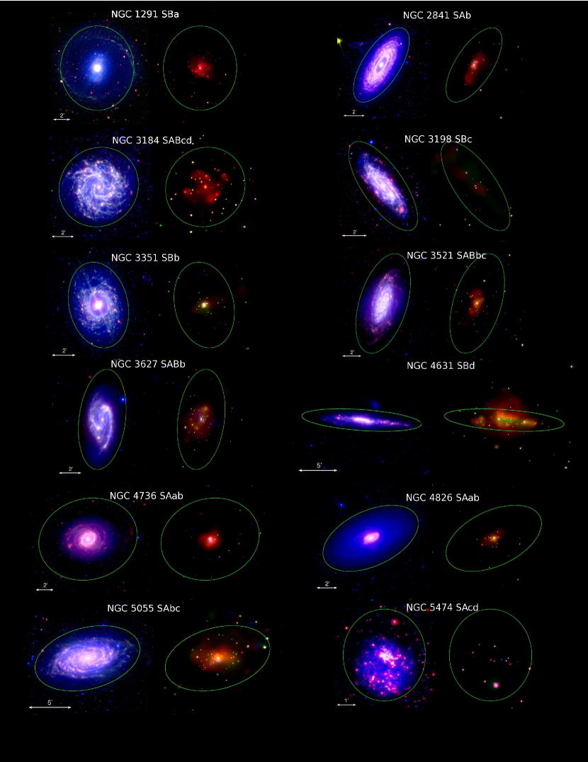
Figure 1.— Infrared morphologies and X-ray point sources of SINGS galaxies in this paper. Each thumbnail pair shows a Spitzer-IRAC composite false-color image at left (blue: 3.6$\mu m$, green: 4.5$\mu m$, red: 8.0$\mu m$) and a Chandra adaptively smoothed false-color composite at right (blue: 0.3-1.0 keV, green: 1.0-2.0 keV, red: 2.0-10.0 keV). The green ellipses indicate the $D_{25}$ isophotes. See Sec. 2 for a brief description of X-ray point-source selection.

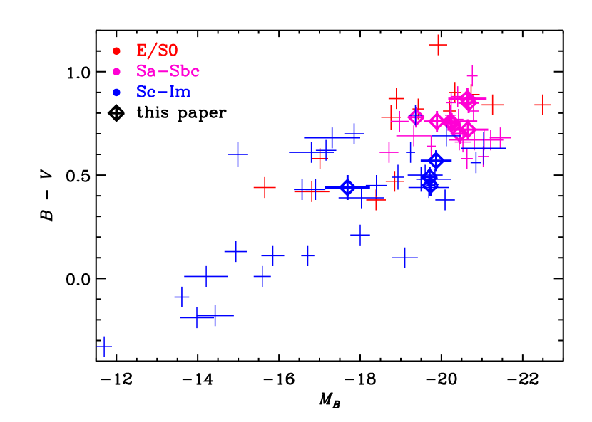
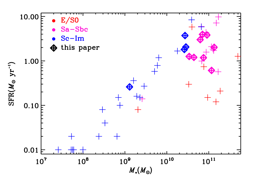
Figure 2.— Properties of our galaxy sample compared to other SINGS galaxies. Left: Color-magnitude diagram. Right: Plot of SFR vs. $M_{\ast}$. In both panels, crosses in normal font indicate SINGS galaxies that are not used in this paper. Bold crosses with diamonds indicate the twelve SINGS galaxies used in this paper. Galaxies are color-coded according to morphology as indicated in the legend. Values in the color-magnitude plot are taken from Moustakas et al. (2010), and in the SFR vs. $M_{\ast}$ plot from Noll et al. (2009).

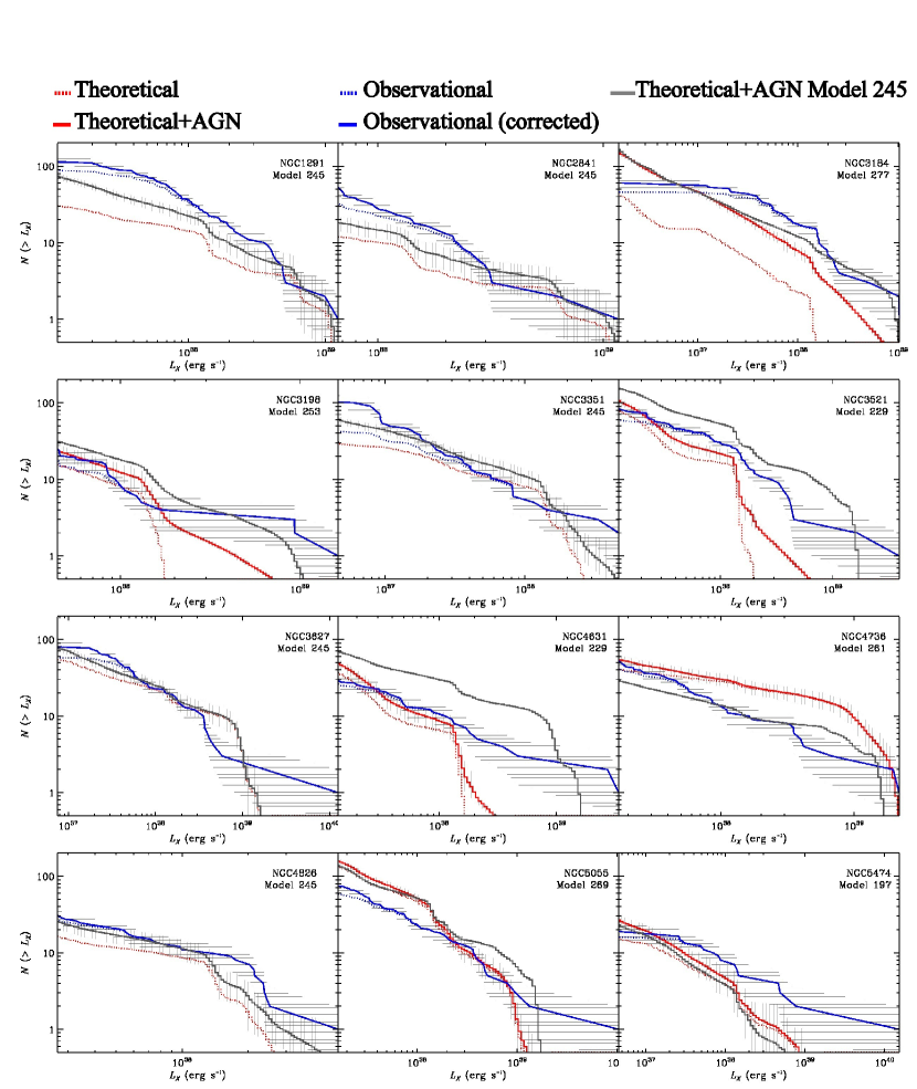
Figure 3.— Observational and theoretical cumulative XLFs for SINGS galaxies. Blue: observational (dotted, original; solid, corrected for incompleteness). Red: theoretical XLF that has highest pair likelihood (Table Modeling X-ray binary evolution in normal galaxies: Insights from SINGS) for a given galaxy (dotted, original; solid, with added expected unrelated contribution from background AGN). Dark grey: theoretical XLF (with added expected AGN contribution) for the galaxy shown, but using StarTrack model 245, which has the highest global likelihood. For galaxies NGC 1291, 2841, 3351, 3627, and 4826 the solid red and solid dark grey curves coincide. The horizontal (vertical) hashed regions indicate $\pm 1\sigma$ estimates for the oXLF and tXLF, respectively, due to Poisson statistics and bolometric uncertainties.

Table 1Model Parameters.

Parameter	Notation	Value	Reference
Initial Orbital Period distribution	$F(P)$	flat in log $\bm{a}$	Abt (1983)
Initial Eccentricity Distribution	$F(e)$	Thermal $\bm{F(e)\sim e}$	Heggie (1975)
Binary Fraction	$f_{\rm bin}$	50%
Magnetic Braking			Ivanova & Taam (2003)
Metallicity	$Z$	0.0001, 0.0002, 0.005, 0.001,
		0.002, 0.005, 0.01, 0.02, 0.03
IMF high-end slope		-2.35 or -2.7	Kroupa (2001); Kroupa & Weidner (2003)
Initial Mass Ratio Distribution	$F(q)$	Flat, twin, or 50% flat – 50% twin	Kobulnicky & Fryer (2007); Pinsonneault & Stanek (2006)
CE Efficiency$\times$ central concentration	$\lambda\alpha_{\rm CE}$	0.1, 0.2, 0.3, 0.5	Podsiadlowski et al. (2003)
Stellar wind strength	$\eta_{\rm wind}$	0.25, 1.0, 2.0	Belczynski et al. (2010)
CE during HG	CE-HG	Yes or No	Belczynski et al. (2007)
SN kick for ECS/AIC NS		20% of normal NS kicks	Linden et al. (2009)
SN kick for direct collapse BH	$\kappa_{\rm DCBH}$	Yes (0.1) or No (0)	Fragos et al. (2010)

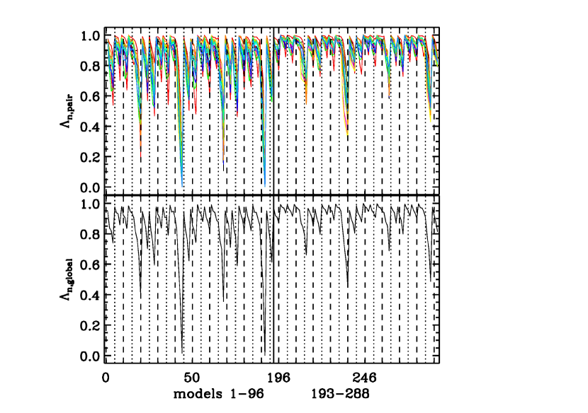
Figure 4.— Normalized pair (top) and global (bottom) likelihood (Sec. 4.3) vs. model number for all models used in this paper. As explained in the text, the global curve in the bottom panel is the combination of the individual curves in the top panel.

Figure 5.— Normalized global likelihood (Sec. 4.3) vs. StarTrack parameter $\lambda\alpha_{\rm CE}$ (donor central concentration $\times$ common envelope efficiency) varied in our model grid. Crosses indicate resistant mean values for normalized global likelihood values of models using a given $\lambda\alpha_{\rm CE}$ value. Error bars indicate $3\sigma$ estimates.

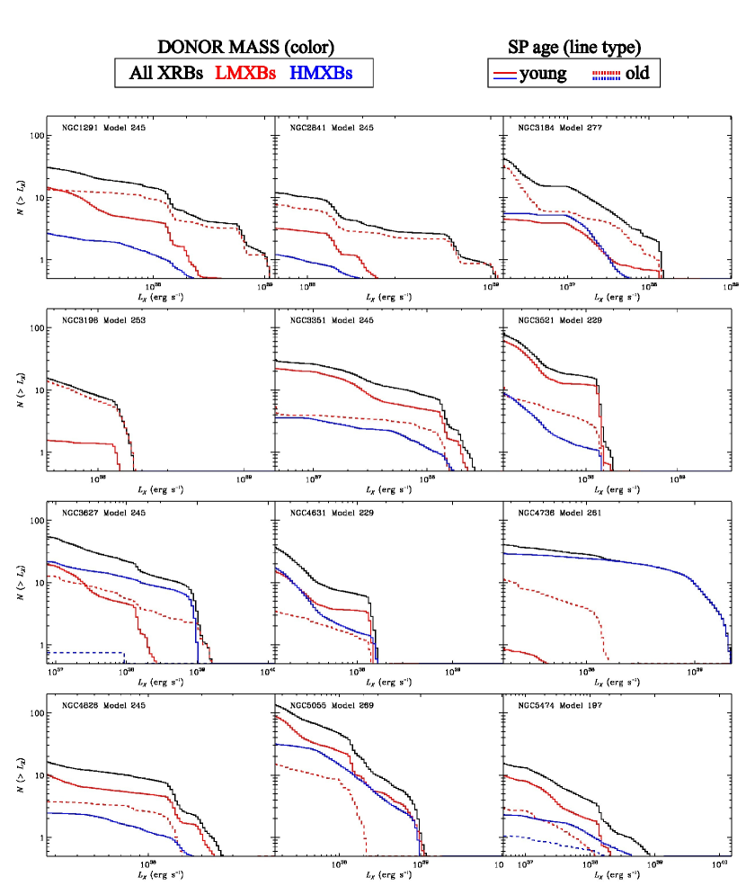
Figure 6.— Cumulative theoretical XLFs for XSINGS galaxies, for subpopulations based on donor mass and age of stellar population. Continuous black curves show the total tXLF (black). The “old” LMXB population is shown by the red dotted lines, and the “old” HMXB population by the blue dotted line. The “young” LMXB population is shown by the red solid line, and the “ young” HMXB population by the blue solid line. The “young” and “old” subpopulations are defined in Noll et al. (2009) and are shown separately by solid and dotted lines, respectively (see also Table Modeling X-ray binary evolution in normal galaxies: Insights from SINGS). Note that the $L_{X}$ axes have different ranges, matching the observed XLF range.

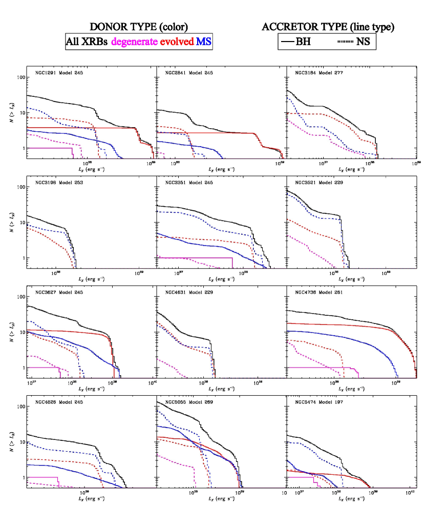
Figure 7.— Cumulative theoretical XLFs for XSINGS galaxies, for subpopulations based on donor and accretor type. The continuous black curve is the total tXLF. For colored curves, color indicates donor stellar type and line type indicates accretor type, as indicated at the top of the figure.

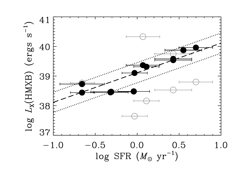
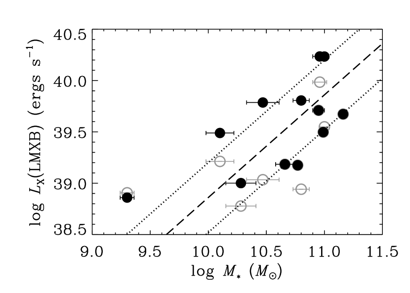
Figure 8.— Integrated $L_{X,{\rm 0.3-10.0keV}}$ from LMXBs and HMXBs from StarTrack modeling vs. SFR and $M_{\ast}$ (Noll et al., 2009) for the 12 SINGS galaxies in this paper. Luminosities have been calculated using both the best pair-likelihood model for each galaxy (open grey circles) and model 245, the best global model in this paper, which is also the top-ranked model in F13 (black filled circles). The dashed line shows the expected contribution from HMXBs (left panel) and LMXBs (right panel) based on the best-fit relation of L10 (Equation 10). The dotted lines show $\pm 1\sigma$ uncertainties.

Table 2SINGS galaxy subsample used in this paper.

Galaxy	$D$	Hubble Type	T-Type	log SFR	log $M_{\ast}$	SSFR	$N_{\rm src}$
	(Mpc)			($M_{\odot}$yr-1)	($M_{\odot}$)	($10^{-11}$ yr-1)
(1)	(2)	(3)	(4)	(5)	(6)	(7)	(8)
NGC1291	10.8	SBa	1	$-0.66\pm 0.27$	$11.16\pm 0.03$	0.151356	88
NGC2841	14.1	SAb	3	$-0.31\pm 0.24$	$10.99\pm 0.03$	0.501187	32
NGC3184	11.1	SABcd	6	$0.11\pm 0.15$	$10.28\pm 0.13$	6.76083	47
NGC3198	13.68	SBc	5	$-0.03\pm 0.15$	$10.10\pm 0.12$	7.4131	19
NGC3351	9.33	SBb	3	$-0.04\pm 0.19$	$10.66\pm 0.08$	1.99526	45
NGC3521	10.1	SABbc	4	$0.43\pm 0.22$	$11.00\pm 0.04$	2.69153	60
NGC3627	9.38	SABb	3	$0.55\pm 0.22$	$10.95\pm 0.05$	3.98107	59
NGC4631	7.62	SBd	7	$0.70\pm 0.20$	$10.47\pm 0.14$	16.9824	29
NGC4736	5.2	SAab	2	$0.07\pm 0.20$	$10.80\pm 0.07$	1.86209	42
NGC4826	7.48	SAab	2	$-0.32\pm 0.21$	$10.77\pm 0.02$	0.812831	28
NGC5055	7.8	SAbc	4	$0.43\pm 0.22$	$10.96\pm 0.06$	2.95121	59
NGC5474	6.8	SAcd	6	$-0.65\pm 0.14$	$9.30\pm 0.06$	11.2202	16

Note. — Columns are: (1) galaxy name; (2) distance (Moustakas et al., 2010); (3) Hubble Type (de Vaucouleurs et al., 1991); (4) T-type; (5) star formation rate from Noll et al. (2009); (6) logarithmic stellar mass from Noll et al. (2009); (7) specific star formation rate (SFR/$M_{\ast}$) from (5) and (6); (8) number of X-ray point sources in XSINGS catalog.

Table 3Star formation histories from SED fitting.

Note. — Best fit values from SED fitting (run B in Noll et al. (2009) and Noll, private communication). Columns are: (1) galaxy name; (2) total stellar mass plus gas mass from stellar mass loss; (3) e-folding timescale for old stellar population; (4) age of old stellar population; (5) e-folding timescale for young stellar population; (6) age of young stellar population; (7) mass fraction of young stellar population.

Table 4Parameters for highest pair-likelihood model-galaxy pairs

Note. — Columns are: (1) galaxy ID; (2) model number; (3) CE efficiency $\times$ central concentration; (4) exponent of high-mass power law component of IMF: Kroupa (2001, $-2.35$) or Kroupa & Weidner (2003, $-2.7$); (5) stellar wind strength parameter; (6) Yes: All possible outcomes of a CE event with a Hertzsprung gap donor allowed; No: A CE with such a donor star will always result to a merger; (7) binary mass ratio distribution: 50-50 means half of the binaries originate in a twin binary distribution and half in a flat mass ratio distribution; (8) parameter with which the Hobbs et al. (2005) kick distribution is multiplied for BHs formed through a SN explosion with negligible ejected mass; (9) rank of best-fit galaxy-model pairs based on pair likelihood value; (10) natural logarithm of ratio of each pair likelihood to maximum pair likelihood in this table: $\ln({\cal L}_{{\rm pair,}km}/{\cal L}_{{\rm pair,}km,{\rm max}})$.

Table 5Parameters and global likelihood values for 15 best models ranked by likelihood.

Note. — Columns are: (1) model number; (2) CE efficiency $\times$ central concentration; (3) exponent of high-mass power law component of IMF: Kroupa (2001, $-2.35$) or Kroupa & Weidner (2003, $-2.7$); (4) stellar wind strength parameter; (5) Yes: All possible outcomes of a CE event with a Hertzsprung gap donor allowed; No: A CE with such a donor star will always result to a merger; (6) binary mass ratio distribution: 50-50 means half of the binaries originate in a twin binary distribution and half in a flat mass ratio distribution; (7) parameter with which the Hobbs et al. (2005) kick distribution is multiplied for BHs formed through a SN explosion with negligible ejected mass; (8) rank of model based on likelihood value in this paper; (9) rank of model based on likelihood value in F13; (10) rank of model based on likelihood value in T13; (11) natural logarithm of ratio of each global likelihood to maximum global likelihood in this table: $\ln(\cal L_{\rm global}/\cal L_{\rm global,max})$. (The full table is available on-line).

Table 6Parameters and global likelihood values for 192 models ranked by likelihood (on-line only).

Note. — Columns are: (1) model number; (2) CE efficiency $\times$ central concentration; (3) exponent of high-mass power law component of IMF: Kroupa (2001, $-2.35$) or Kroupa & Weidner (2003, $-2.7$); (4) stellar wind strength parameter; (5) Yes: All possible outcomes of a CE event with a Hertzsprung gap donor allowed; No: A CE with such a donor star will always result to a merger; (6) binary mass ratio distribution: 50-50 means half of the binaries originate in a twin binary distribution and half in a flat mass ratio distribution; (7) parameter with which the Hobbs et al. (2005) kick distribution is multiplied for BHs formed through a SN explosion with negligible ejected mass; (8) rank of model based on likelihood value in this paper; (9) rank of model based on likelihood value in F13; (10) rank of model based on likelihood value in T13; (11) natural logarithm of ratio of each global likelihood to maximum global likelihood in this table: $\ln(\cal L_{\rm global}/\cal L_{\rm global,max})$. (The full table is available on-line).

References

- Abt (1983) Abt, H. A. 1983, ARA&A, 21, 343
- Bastian et al. (2010) Bastian, N., Covey, K. R., & Meyer, M. R. 2010, ARA&A, 48, 339
- Belczynski et al. (2010) Belczynski, K., Bulik, T., Fryer, C. L., Ruiter, A., Valsecchi, F., Vink, J. S., & Hurley, J. R. 2010, ApJ, 714, 1217
- Belczynski et al. (2002) Belczynski, K., Bulik, T., & Rudak, B. 2002, ApJ, 571, 394
- Belczynski et al. (2008) Belczynski, K., Kalogera, V., Rasio, F. A., Taam, R. E., Zezas, A., Bulik, T., Maccarone, T. J., & Ivanova, N. 2008, ApJS, 174, 223
- Belczynski et al. (2004) Belczynski, K., Kalogera, V., Zezas, A., & Fabbiano, G. 2004, ApJ, 601, L147
- Belczynski et al. (2007) Belczynski, K., Taam, R. E., Kalogera, V., Rasio, F. A., & Bulik, T. 2007, ApJ, 662, 504
- Belczynski et al. (2012) Belczynski, K., Wiktorowicz, G., Fryer, C. L., Holz, D. E., & Kalogera, V. 2012, ApJ, 757, 91
- Bhadkamkar & Ghosh (2012) Bhadkamkar, H., & Ghosh, P. 2012, ApJ, 746, 22
- Bhadkamkar & Ghosh (2013a) —. 2013a, astro-ph/1301.1269
- Bhadkamkar & Ghosh (2013b) —. 2013b, astro-ph/1301.1283
- Binder et al. (2013) Binder, B., Williams, B. F., Eracleous, M., Gaetz, T. J., Kong, A. K. H., Skillman, E. D., & Weisz, D. R. 2013, ApJ, 763, 128
- Binder et al. (2012) Binder, B., Williams, B. F., Eracleous, M., Gaetz, T. J., Plucinsky, P. P., Skillman, E. D., Dalcanton, J. J., Anderson, S. F., Weisz, D. R., & Kong, A. K. H. 2012, ApJ, 758, 15
- Bogdán & Gilfanov (2010) Bogdán, Á., & Gilfanov, M. 2010, A&A, 512, A16
- Boroson et al. (2011) Boroson, B., Kim, D.-W., & Fabbiano, G. 2011, The Astrophysical Journal, 729, 12
- Broos et al. (2010) Broos, P. S., Townsley, L. K., Feigelson, E. D., Getman, K. V., Bauer, F. E., & Garmire, G. P. 2010, ApJ, 714, 1582
- Dalcanton et al. (2009) Dalcanton, J. J., Williams, B. F., Seth, A. C., Dolphin, A., Holtzman, J., Rosema, K., Skillman, E. D., Cole, A., Girardi, L., Gogarten, S. M., Karachentsev, I. D., Olsen, K., Weisz, D., Christensen, C., Freeman, K., Gilbert, K., Gallart, C., Harris, J., Hodge, P., de Jong, R. S., Karachentseva, V., Mateo, M., Stetson, P. B., Tavarez, M., Zaritsky, D., Governato, F., & Quinn, T. 2009, ApJS, 183, 67
- de Vaucouleurs et al. (1991) de Vaucouleurs, G., de Vaucouleurs, A., Corwin, H. G., Buta, R. J., Paturel, G., & Fouque, P. 1991, Third Reference Catalogue of Bright Galaxies (Volume 1-3, XII, 2069 pp. 7 figs. Springer-Verlag Berlin Heidelberg New York)
- Dobrotka et al. (2006) Dobrotka, A., Lasota, J.-P., & Menou, K. 2006, ApJ, 640, 288
- Dominik et al. (2012) Dominik, M., Belczynski, K., Fryer, C., Holz, D. E., Berti, E., Bulik, T., Mandel, I., & O’Shaughnessy, R. 2012, ApJ, 759, 52
- Dubus et al. (1999) Dubus, G., Lasota, J.-P., Hameury, J.-M., & Charles, P. 1999, MNRAS, 303, 139
- Duquennoy & Mayor (1991) Duquennoy, A., & Mayor, M. 1991, A&A, 248, 485
- Eracleous et al. (2006) Eracleous, M., Sipior, M. S., & Sigurdsson, S. 2006, in IAU Symposium, Vol. 230, Populations of High Energy Sources in Galaxies, ed. E. J. A. Meurs & G. Fabbiano, 417–422
- Fabbiano (2006) Fabbiano, G. 2006, ARA&A, 44, 323
- Fan et al. (1996) Fan, X., Burstein, D., Chen, J.-S., Zhu, J., Jiang, Z., Wu, H., Yan, H., Zheng, Z., Zhou, X., Fang, L.-Z., Chen, F., Deng, Z., Chu, Y., Hester, J. J., Windhorst, R. A., Li, Y., Lu, P., Sun, W.-H., Chen, W.-P., Tsay, W.-S., Chiueh, T.-H., Chou, C.-K., Ko, C.-M., Lin, T.-C., Guo, H.-J., & Byun, Y.-I. 1996, AJ, 112, 628
- Fischer & Marcy (1992) Fischer, D. A., & Marcy, G. W. 1992, ApJ, 396, 178
- Fragos et al. (2008) Fragos, T., Kalogera, V., Belczynski, K., Fabbiano, G., Kim, D.-W., Brassington, N. J., Angelini, L., Davies, R. L., Gallagher, J. S., King, A. R., Pellegrini, S., Trinchieri, G., Zepf, S. E., Kundu, A., & Zezas, A. 2008, ApJ, 683, 346
- Fragos et al. (2009) Fragos, T., Kalogera, V., Willems, B., Belczynski, K., Fabbiano, G., Brassington, N. J., Kim, D.-W., Angelini, L., Davies, R. L., Gallagher, J. S., King, A. R., Pellegrini, S., Trinchieri, G., Zepf, S. E., & Zezas, A. 2009, ApJ, 702, L143
- Fragos et al. (2013) Fragos, T., Lehmer, B., Tremmel, M., Tzanavaris, P., Basu-Zych, A., Belczynski, K., Hornschemeier, A., Jenkins, L., Kalogera, V., Ptak, A., & Zezas, A. 2013, ApJ, 764, 41
- Fragos et al. (2010) Fragos, T., Tremmel, M., Rantsiou, E., & Belczynski, K. 2010, ApJ, 719, L79
- Fryer et al. (2012) Fryer, C. L., Belczynski, K., Wiktorowicz, G., Dominik, M., Kalogera, V., & Holz, D. E. 2012, ApJ, 749, 91
- Ghosh & White (2001) Ghosh, P., & White, N. E. 2001, ApJ, 559, L97
- Gilfanov (2004) Gilfanov, M. 2004, MNRAS, 349, 146
- Gilfanov et al. (2004) Gilfanov, M., Grimm, H.-J., & Sunyaev, R. 2004, MNRAS, 347, L57
- Greggio et al. (2012) Greggio, L., Falomo, R., Zaggia, S., Fantinel, D., & Uslenghi, M. 2012, PASP, 124, 653
- Grimm et al. (2003) Grimm, H.-J., Gilfanov, M., & Sunyaev, R. 2003, MNRAS, 339, 793
- Guo et al. (2011) Guo, Q., White, S., Boylan-Kolchin, M., De Lucia, G., Kauffmann, G., Lemson, G., Li, C., Springel, V., & Weinmann, S. 2011, MNRAS, 413, 101
- Heggie (1975) Heggie, D. C. 1975, MNRAS, 173, 729
- Hobbs et al. (2005) Hobbs, G., Lorimer, D. R., Lyne, A. G., & Kramer, M. 2005, MNRAS, 360, 974
- Hurley et al. (2007) Hurley, J. R., Aarseth, S. J., & Shara, M. M. 2007, ApJ, 665, 707
- Hurley et al. (2000) Hurley, J. R., Pols, O. R., & Tout, C. A. 2000, MNRAS, 315, 543
- Hurley et al. (2002) Hurley, J. R., Tout, C. A., & Pols, O. R. 2002, MNRAS, 329, 897
- Hurley et al. (2010) Hurley, J. R., Tout, C. A., Wickramasinghe, D. T., Ferrario, L., & Kiel, P. D. 2010, MNRAS, 402, 1437
- Ivanova et al. (2005) Ivanova, N., Belczynski, K., Fregeau, J. M., & Rasio, F. A. 2005, MNRAS, 358, 572
- Ivanova & Taam (2003) Ivanova, N., & Taam, R. E. 2003, ApJ, 599, 516
- Jenkins et al. (2010) Jenkins, L., Hornschemeier, A., Zezas, A., Gallagher, S., Dale, D., Calzetti, D., Ptak, A., Strickland, D., Kuntz, K., & Kalogera, V. 2010, in Bulletin of the American Astronomical Society, Vol. 42, AAS/High Energy Astrophysics Division #11, 700
- Kennicutt et al. (2003) Kennicutt, Jr., R. C., Armus, L., Bendo, G., Calzetti, D., Dale, D. A., Draine, B. T., Engelbracht, C. W., Gordon, K. D., Grauer, A. D., Helou, G., Hollenbach, D. J., Jarrett, T. H., Kewley, L. J., Leitherer, C., Li, A., Malhotra, S., Regan, M. W., Rieke, G. H., Rieke, M. J., Roussel, H., Smith, J.-D. T., Thornley, M. D., & Walter, F. 2003, PASP, 115, 928
- Kiel & Hurley (2006) Kiel, P. D., & Hurley, J. R. 2006, MNRAS, 369, 1152
- Kim & Fabbiano (2003) Kim, D.-W., & Fabbiano, G. 2003, ApJ, 586, 826
- Kim & Fabbiano (2004) —. 2004, ApJ, 611, 846
- Kim et al. (1992) Kim, D.-W., Fabbiano, G., & Trinchieri, G. 1992, ApJ, 393, 134
- Kim et al. (2007) Kim, M., Wilkes, B. J., Kim, D.-W., Green, P. J., Barkhouse, W. A., Lee, M. G., Silverman, J. D., & Tananbaum, H. D. 2007, ApJ, 659, 29
- King et al. (1996) King, A. R., Kolb, U., & Burderi, L. 1996, ApJ, 464, L127
- Kobulnicky & Fryer (2007) Kobulnicky, H. A., & Fryer, C. L. 2007, ApJ, 670, 747
- Kong et al. (2002) Kong, A. K. H., Garcia, M. R., Primini, F. A., Murray, S. S., Di Stefano, R., & McClintock, J. E. 2002, ApJ, 577, 738
- Kroupa (2001) Kroupa, P. 2001, MNRAS, 322, 231
- Kroupa (2012) —. 2012, in Stellar Systems and Galactic Structure, Vol. 5, Springer; astroph/1112.3340
- Kroupa & Weidner (2003) Kroupa, P., & Weidner, C. 2003, ApJ, 598, 1076
- Lehmer et al. (2010) Lehmer, B. D., Alexander, D. M., Bauer, F. E., Brandt, W. N., Goulding, A. D., Jenkins, L. P., Ptak, A., & Roberts, T. P. 2010, ApJ, 724, 559
- Linden et al. (2010) Linden, T., Kalogera, V., Sepinsky, J. F., Prestwich, A., Zezas, A., & Gallagher, J. S. 2010, ApJ, 725, 1984
- Linden et al. (2009) Linden, T., Sepinsky, J. F., Kalogera, V., & Belczynski, K. 2009, ApJ, 699, 1573
- Lipunov et al. (1996) Lipunov, V. M., Ozernoy, L. M., Popov, S. B., Postnov, K. A., & Prokhorov, M. E. 1996, ApJ, 466, 234
- Lipunov et al. (2009) Lipunov, V. M., Postnov, K. A., Prokhorov, M. E., & Bogomazov, A. I. 2009, Astronomy Reports, 53, 915
- Lü et al. (2012) Lü, G.-L., Zhu, C.-H., Postnov, K. A., Yungelson, L. R., Kuranov, A. G., & Wang, N. 2012, MNRAS, 424, 2265
- Luo et al. (2012) Luo, B., Fabbiano, G., Fragos, T., Kim, D.-W., Belczynski, K., Brassington, N. J., Pellegrini, S., Tzanavaris, P., Wang, J., & Zezas, A. 2012, ApJ, 749, 130
- Luo et al. (2013) Luo, B., Fabbiano, G., Strader, J., Kim, D.-W., Brodie, J. P., Fragos, T., Gallagher, J. S., King, A., & Zezas, A. 2013, ApJS, 204, 14
- Mineo et al. (2012) Mineo, S., Gilfanov, M., & Sunyaev, R. 2012, MNRAS, 419, 2095
- Moustakas et al. (2010) Moustakas, J., Kennicutt, Jr., R. C., Tremonti, C. A., Dale, D. A., Smith, J.-D. T., & Calzetti, D. 2010, ApJS, 190, 233
- Noll et al. (2009) Noll, S., Burgarella, D., Giovannoli, E., Buat, V., Marcillac, D., & Muñoz-Mateos, J. C. 2009, A&A, 507, 1793
- Persic & Rephaeli (2007) Persic, M., & Rephaeli, Y. 2007, A&A, 463, 481
- Pfahl et al. (2003) Pfahl, E., Rappaport, S., & Podsiadlowski, P. 2003, ApJ, 597, 1036
- Pinsonneault & Stanek (2006) Pinsonneault, M. H., & Stanek, K. Z. 2006, ApJ, 639, L67
- Piro & Bildsten (2002) Piro, A. L., & Bildsten, L. 2002, ApJ, 571, L103
- Podsiadlowski et al. (2003) Podsiadlowski, P., Rappaport, S., & Han, Z. 2003, MNRAS, 341, 385
- Raghavan et al. (2010) Raghavan, D., McAlister, H. A., Henry, T. J., Latham, D. W., Marcy, G. W., Mason, B. D., Gies, D. R., White, R. J., & ten Brummelaar, T. A. 2010, ApJS, 190, 1
- Ranalli et al. (2003) Ranalli, P., Comastri, A., & Setti, G. 2003, A&A, 399, 39
- Rejkuba et al. (2009) Rejkuba, M., Mouhcine, M., & Ibata, R. 2009, MNRAS, 396, 1231
- Revnivtsev et al. (2008) Revnivtsev, M., Lutovinov, A., Churazov, E., Sazonov, S., Gilfanov, M., Grebenev, S., & Sunyaev, R. 2008, A&A, 491, 209
- Revnivtsev et al. (2011) Revnivtsev, M., Postnov, K., Kuranov, A., & Ritter, H. 2011, A&A, 526, A94
- Sana et al. (2012) Sana, H., de Mink, S. E., de Koter, A., Langer, N., Evans, C. J., Gieles, M., Gosset, E., Izzard, R. G., Le Bouquin, J.-B., & Schneider, F. R. N. 2012, Science, 337, 444
- Scalo (1986) Scalo, J. M. 1986, Fund. Cosmic Phys., 11, 1
- Sepinsky et al. (2005) Sepinsky, J., Kalogera, V., & Belczynski, K. 2005, ApJ, 621, L37
- Shtykovskiy & Gilfanov (2007) Shtykovskiy, P. E., & Gilfanov, M. R. 2007, Astronomy Letters, 33, 437
- Sivakoff et al. (2003) Sivakoff, G. R., Sarazin, C. L., & Irwin, J. A. 2003, ApJ, 599, 218
- Soria & Kong (2002) Soria, R., & Kong, A. K. H. 2002, ApJ, 572, L33
- Tanaka & Shibazaki (1996) Tanaka, Y., & Shibazaki, N. 1996, ARA&A, 34, 607
- Tikhonov & Galazutdinova (2012) Tikhonov, N. A., & Galazutdinova, O. A. 2012, Astronomy Letters, 38, 147
- Trudolyubov et al. (2002) Trudolyubov, S. P., Borozdin, K. N., Priedhorsky, W. C., Mason, K. O., & Cordova, F. A. 2002, ApJ, 571, L17
- Tzanavaris & Georgantopoulos (2008) Tzanavaris, P., & Georgantopoulos, I. 2008, A&A, 480, 663
- White & Ghosh (1998) White, N. E., & Ghosh, P. 1998, ApJ, 504, L31+
- Wu (2001) Wu, K. 2001, PASA, 18, 443
- Zezas & Fabbiano (2002) Zezas, A., & Fabbiano, G. 2002, ApJ, 577, 726
- Zezas et al. (2007) Zezas, A., Fabbiano, G., Baldi, A., Schweizer, F., King, A. R., Rots, A. H., & Ponman, T. J. 2007, ApJ, 661, 135
- Zhang et al. (2012) Zhang, Z., Gilfanov, M., & Bogdán, Á. 2012, A&A, 546, A36
- Zhang et al. (2011) Zhang, Z., Gilfanov, M., Voss, R., Sivakoff, G. R., Kraft, R. P., Brassington, N. J., Kundu, A., Jordán, A., & Sarazin, C. 2011, A&A, 533, A33
- Zuo & Li (2011) Zuo, Z.-Y., & Li, X.-D. 2011, ApJ, 733, 5