Universality Class in Conformal Inflation

Renata Kallosh and Andrei Linde

Department of Physics and SITP, Stanford University, Stanford, California 94305 USA

We develop a new class of chaotic inflation models with spontaneously broken conformal invariance. Observational consequences of a broad class of such models are stable with respect to strong deformations of the scalar potential. This universality is a critical phenomenon near the point of enhanced symmetry, $SO(1,1)$, in case of conformal inflation. It appears because of the exponential stretching of the moduli space and the resulting exponential flattening of scalar potentials upon switching from the Jordan frame to the Einstein frame in this class of models. This result resembles stretching and flattening of inhomogeneities during inflationary expansion. It has a simple interpretation in terms of velocity versus rapidity near the Kähler cone in the moduli space, similar to the light cone of special theory of relativity. This effect makes inflation possible even in the models with very steep potentials. We describe conformal and superconformal versions of this cosmological attractor mechanism.

1 Introduction

This paper extends the series of our recent papers [1, 2] where we developed a superconformal approach to the description of a broad class of models favored by observational data from WMAP9 [3] and Planck2013 [4]. The superconformal approach to cosmology is based on earlier papers [5, 6, 7].

Recent observational data attracted attention of cosmologists to a class of inflationary models which made very similar observational predictions, even though their formulations could seem entirely unrelated to each other. This includes the early model [8], with main observational predictions derived in [9]. The same observational predictions were made in the context of chaotic inflation in the theory $\lambda\phi^{4}$ [10] with non-minimal coupling to gravity ${\xi\over 2}\phi^{2}R$ with $\xi>0$ [11, 12], in its supersymmetric extensions in [13, 6, 14, 7] and in a certain limit of the model with the Higgs potential with $\xi<0$ [15]. Recently another set of models with similar predictions was identified in [16, 1, 2, 17].

Relation of these models to each other remained quite mysterious. In our recent set of papers [1, 2] we proposed that spontaneously broken superconformal symmetry is useful to describe these and other inflationary models favored by observations. In this paper we will describe a new class of models of inflation suggested by the framework of conformal and superconformal symmetry. These new models form a universality class. In terms of the observational data, they all have an attractor point

$$1-n_{s}=2/N\,,\qquad r=12/N^{2}$$ (1.1)

in the leading approximation in $1/N$, where $N$ is the number of e-folding of inflation. This class of models is very broad; it includes the Starobinsky model as well as the Higgs model with $\xi<0$. The same attractor point (1.1) corresponds to Higgs inflation type models with $\xi>0$, but they form a different universality class, as discussed in [1].

The class of models we study depends on two scalar fields. The action has a local conformal symmetry, one field $\chi$ we call a conformon, following [5], where the superconformal approach to cosmology was first developed. The other field $\phi$ is an inflaton. Local conformal symmetry for these two fields in absence of a potential has an unbroken global $SO(1,1)$ symmetry. The potential can be added which preserves $SO(1,1)$ symmetry as well as a local conformal symmetry. This form a critical point of the system, which is a dS/AdS space, depending on the sign of the potential.

A small deformation of $SO(1,1)$ symmetry for all of our models corresponds to deforming the $SO(1,1)$ conformally invariant potential by an arbitrary function $F(\phi/\chi)$, which is a unique way of preserving local conformal symmetry. The simplest representative of this class of theories is $F(\phi/\chi)\sim(\phi/\chi)^{2}$; we called it the T-Model for the reasons to become apparent later. As we have shown in [2], a more complicated function $F(\phi/\chi)\sim{(\phi/\chi)^{2}\over 1+(\phi/\chi)^{2}}$ corresponds to the Starobinsky model. We will show that these models and their numerous generalizations belong to the same universality class of slightly $SO(1,1)$ deformed models, which has an attractor point (1.1).

In section 2 of this paper we present examples of actions with local conformal symmetry in presence of the conformon field, which lead to dS or AdS spaces when conformal symmetry is spontaneously broken. We use two types of gauges to fix conformal symmetry, which lead to the same results in the Einstein frame. These gauges are related to each other as velocity and rapidity in special theory of relativity and have different advantages for various purposes, which we use later in more interesting models. In section 3 we introduce a new class of inflationary models, the basic one we call T-Model, as a deviation from the $SO(1,1)$ invariant conformal models with de Sitter geometry. We find that their cosmological evolution is universal in the first approximation in $1/N$ where $N$ is the number of e-foldings, due to an exponential stretching and flattening of the inflaton potential near the boundary of the moduli space. In section 4 we investigate more general class of conformal inflation models, which have an analogous attractor behavior for slow roll inflation parameters and flattening of the inflationary potentials. In section 5 we describe a supersymmetric generalization of the universality class of conformal inflation, and in section 6 we present some comments on general emergence of critical phenomena in the superconformal approach to cosmology.

2 de Sitter from spontaneously broken conformal symmetry

2.1 The simplest conformally invariant one-field model of dS/AdS space

As a first step towards the development of the new class of inflationary models based on spontaneously broken conformal symmetry, consider a simple conformally invariant model of gravity of a scalar field $\chi$ with the following Lagrangian

$$\mathcal{L}=\sqrt{-{g}}\left[{1\over 2}\partial_{\mu}\chi\partial_{\nu}\chi\,g^{\mu\nu}+{\chi^{2}\over 12}R({g})-{\lambda\over 4}\chi^{4}\right]\,.$$ (2.1)

This theory is locally conformal invariant under the following transformations:

$$\tilde{g}_{\mu\nu}={\rm e}^{-2\sigma(x)}g_{\mu\nu}\,,\qquad\tilde{\chi}={\rm e}^{\sigma(x)}\chi\ .$$ (2.2)

The field $\chi(x)$ is referred to as a conformal compensator, which we will call ‘conformon.’ It has negative sigh kinetic term, but this is not a problem because it can be removed from the theory by fixing the gauge symmetry (2.6), for example by taking a gauge $\chi=\sqrt{6}$. This gauge fixing can be interpreted as a spontaneous breaking of conformal invariance due to existence of a classical field $\chi=\sqrt{6}$.

After fixing $\chi=\sqrt{6}$ the interaction term $-{\lambda\over 4}\chi^{4}$ becomes a cosmological constant $\Lambda={9}\lambda$

$$\mathcal{L}=\sqrt{-{g}}\,\left[{R({g})\over 2}-{9\lambda}\right]\,.$$ (2.3)

For $\lambda>0$, this theory has a simple de Sitter solution

$$a(t)=e^{Ht}=e^{\sqrt{\Lambda/3}\ t}=e^{\sqrt{3\lambda}\ t}.$$ (2.4)

Meanwhile for $\lambda<0$ it becomes the AdS universe with a negative cosmological constant.

2.2 The simplest conformally invariant two-field model of dS/AdS space

Consider now the model of two real scalar fields, $\phi$ and $\chi$, which has also an $SO(1,1)$ symmetry:

$$\mathcal{L}_{\rm toy}=\sqrt{-{g}}\left[{1\over 2}\partial_{\mu}\chi\partial^{\mu}\chi+{\chi^{2}\over 12}R({g})-{1\over 2}\partial_{\mu}\phi\partial^{\mu}\phi-{\phi^{2}\over 12}R({g})-{\lambda\over 4}(\phi^{2}-\chi^{2})^{2}\right]\,.$$ (2.5)

This theory is locally conformal invariant under the following transformations:

$$\tilde{g}_{\mu\nu}={\rm e}^{-2\sigma(x)}g_{\mu\nu}\,,\qquad\tilde{\chi}={\rm e}^{\sigma(x)}\chi\,,\qquad\tilde{\phi}={\rm e}^{\sigma(x)}\phi\ .$$ (2.6)

The global $SO(1,1)$ symmetry is a boost between these two fields.

2.3 $SO(1,1)$ invariant conformal gauge: rapidity gauge $\chi^{2}-\phi^{2}=6$

Because of this symmetry, it is very convenient to choose an $SO(1,1)$ invariant conformal gauge,

$$\chi^{2}-\phi^{2}=6\ ,$$ (2.7)

which reflects the $SO(1,1)$ invariance of our model. This gauge condition (we will refer to it as a ‘rapidity’ gauge) represents a hyperbola which can be parametrized by a canonically normalized field $\varphi$

$$\chi=\sqrt{6}\cosh{\varphi\over\sqrt{6}}\,,\qquad\phi=\sqrt{6}\sinh{\varphi\over\sqrt{6}}\ .$$ (2.8)

This allows us to modify the kinetic term into a canonical one for the independent field $\varphi$

$${1\over 2}\partial_{\mu}\chi\partial^{\mu}\chi-{1\over 2}\partial_{\mu}\phi\partial^{\mu}\phi\,\quad\Rightarrow\quad{1\over 2}\partial_{\mu}\varphi\partial^{\mu}\varphi$$ (2.9)

and the non-minimal curvature coupling into a minimal one

$${\chi^{2}\over 12}R({g})-{\phi^{2}\over 12}R({g})\,\quad\Rightarrow\quad{1\over 2}R({g})\,.$$ (2.10)

Using the standard terminology of special relativity, including the concept of rapidity, we may define ${\chi\over\sqrt{6}}=\cosh{\varphi\over\sqrt{6}}=\gamma\,,{\phi\over\sqrt{6}}=\sinh{\varphi\over\sqrt{6}}=\gamma{v\over c}$ and

$$\tanh{\varphi\over\sqrt{6}}={v\over c}\ .$$ (2.11)

For low speeds, rapidity and speed are proportional, but for high speeds, rapidity takes a larger value. We see that the canonically normalized inflaton is related to ‘rapidity’ $\theta=\tanh^{-1}{v\over c}$ as follows

$$\theta={\varphi\over\sqrt{6}}\ .$$ (2.12)

In this gauge the Higgs-type potential ${\lambda\over 4}(\phi^{2}-\chi^{2})^{2}$ turns out to be a cosmological constant $9\lambda$, and our action (2.5) becomes

$$L=\sqrt{-g}\left[\frac{1}{2}R-\frac{1}{2}\partial_{\mu}\varphi\partial^{{\mu}}\varphi-9\lambda\right].$$ (2.13)

This theory has the constant potential $V=9\lambda$. Therefore this model can describe de Sitter expansion with the Hubble constant $H^{2}=3\lambda$, for positive $\lambda$. For negative $\lambda$ in (2.5) the model can describe an AdS space. But unlike the one-field model, this model also describes a massless scalar field $\varphi$, which may have its kinetic and gradient energy. If one takes this energy into account, the universe approaches dS regime as soon as expansion of the universe makes the kinetic and gradient energy of the field $\varphi$ sufficiently small.

2.4 $\chi(x)=\sqrt{6}$ conformal gauge

One can also describe the model (2.5) differently. One may chose to fix the local conformal symmetry by using the gauge $\chi(x)=\sqrt{6}$.The full Lagrangian in the Jordan frame becomes

$$\mathcal{L}_{\rm total}=\sqrt{-{g_{J}}}\,\left[{R({g_{J}})\over 2}\left(1-{\phi^{2}\over 6}\right)-{1\over 2}\partial_{\mu}\phi\partial^{\mu}\phi-{\lambda\over 4}\left(\phi^{2}-6\right)^{2}\right]\,.$$ (2.14)

Now one can represent the same theory in the Einstein frame, by changing the metric $g_{J}$ and $\phi$ to a conformally related metric $g_{E}^{\mu\nu}=(1-\phi^{2}/6)^{{-1}}g_{J}^{\mu\nu}$ and a new canonically normalized field $\varphi$ related to the field $\phi$ as follows:

$$\frac{d\varphi}{d\phi}={1\over 1-{\phi^{2}/6}}\ .$$ (2.15)

In new variables, the Lagrangian, up to a total derivative, is given by

$$L=\frac{1}{2}\sqrt{-g}\left[R-\frac{1}{2}g^{\mu\nu}\partial_{\mu}\varphi\partial_{\nu}\varphi-V(\phi(\varphi))\right].$$ (2.16)

where the potential in the Einstein frame is

$$V(\phi)={\lambda\over 4}{\left(\phi^{2}-6\right)^{2}\over\left(1-{\phi^{2}\over 6}\right)^{2}}=9\lambda\ .$$ (2.17)

This finally brings the theory to the form which was found earlier in (2.13).

Here the relation between the gauges $\chi^{2}(x)-\phi^{2}(x)=6$ and $\chi(x)=\sqrt{6}$ corresponds to a relation between rapidity and velocity. The first in (2.13) brings us to an Einstein frame, the second one first brings us to a Jordan frame (2.14). After switching from the Jordan frame to the Einstein one finds a complete agreement. This is expected since rapidity is an alternative to speed description of a motion.

3 Chaotic inflation from conformal theory: T-Model

Now we will consider a conformally invariant class of models

$$\mathcal{L}=\sqrt{-{g}}\left[{1\over 2}\partial_{\mu}\chi\partial^{\mu}\chi+{\chi^{2}\over 12}R({g})-{1\over 2}\partial_{\mu}\phi\partial^{\mu}\phi-{\phi^{2}\over 12}R({g})-{1\over 36}F\left({\phi/\chi}\right)(\phi^{2}-\chi^{2})^{2}\right]\,.$$ (3.1)

where $F$ is an arbitrary function of the ratio ${\phi\over\chi}$. When this function is present, it breaks the $SO(1,1)$ symmetry of the de Sitter model (2.5). Note that this is the only possibility to keep local conformal symmetry and to deform the $SO(1,1)$ symmetry: an arbitrary function $F\left({\phi/\chi}\right)$ has to deviate from the critical value $F\left({\phi/\chi}\right)=\rm const$, where $SO(1,1)$ symmetry is restored.

This theory has the same conformal invariance as the theories considered earlier. As before, we may use the gauge $\chi^{2}-\phi^{2}=6$ and resolve this constraint in terms of the fields $\chi=\sqrt{6}\cosh{\varphi\over\sqrt{6}}$, $\phi=\sqrt{6}\sinh{\varphi\over\sqrt{6}}$ and the canonically normalized field $\varphi={\phi\over\chi}=\tanh{\varphi\over\sqrt{6}}$. Our action (3.1) becomes

$$L=\sqrt{-g}\left[\frac{1}{2}R-\frac{1}{2}\partial_{\mu}\varphi\partial^{\mu}\varphi-F(\tanh{\varphi\over\sqrt{6}})\right].$$ (3.2)

Note that asymptotically $\tanh\varphi\rightarrow\pm 1$ and therefore $F(\tanh{\varphi\over\sqrt{6}})\rightarrow\rm const$, the system in large $\varphi$ limit evolves asymptotically towards its critical point where the $SO(1,1)$ symmetry is restored.

Since $F\left({\phi/\chi}\right)$ is an arbitrary function, by a proper choice of this function one can reproduce an arbitrary chaotic inflation potential $V(\varphi)$ in terms of a conformal theory with spontaneously broken conformal invariance. But this would look rather artificial. For example, to find a theory which has potential $m^{2}\varphi^{2}/2$ in terms of the canonically normalized field $\varphi$, one would need to use $F(\phi)\sim(\tanh^{{-1}}\phi)^{2}$, which is a possible but rather peculiar choice in the context of this class of theories.

Alternatively, one may think about the function $F\left({\phi/\chi}\right)$ as describing a deviation of inflationary theory from the pure cosmological constant potential which emerges in the theory (2.5) with the coupling $(\phi^{2}-\chi^{2})^{2}$. Therefore it is interesting to study what will happen if one takes the simplest set of functions $F\left({\phi/\chi}\right)=\lambda\left({\phi/\chi}\right)^{2n}$ as we did in the standard approach to chaotic inflation.

In this case one finds

$$V(\varphi)=\lambda_{n}\ {\tanh}^{2n}(\varphi/\sqrt{6}).$$ (3.3)

This is a basic representative of the universality class of models depending on $\tanh(\varphi/\sqrt{6})$. We will call it a T-Model, because it originates from different powers of $\tanh(\varphi/\sqrt{6})$, and also because its basic representative $\lambda_{1}\ {\tanh}^{2}(\varphi/\sqrt{6})$ is the simplest version of the class of conformal chaotic inflation models considered in this paper. Moreover, as we will see, observational predictions of a very broad class of models of this type, including their significantly modified and deformed cousins, have nearly identical observational consequences, thus belonging to the same universality class. As Henry Ford famously exclaimed with respect to the T-Model Ford: “Any customer can have a car painted any color that he wants so long as it is black.”

Figure 1: Potentials for the T-Model inflation ${\tanh}^{2n}(\varphi/\sqrt{6})$ for $n=1,2,3,4$ (blue, red, brown and green, corresponding to increasingly wider potentials). We took $\lambda_{n}=1$ for each of the potential for convenience of comparison. As we see, these potentials differ from each other quite considerably, especially at $\varphi\lesssim 1$: at small $\phi$ they behave as $\varphi^{2n}$. Nevertheless all of these models predict the same values $n_{s}=1-2/N$, $r=12/N^{2}$, in the leading approximation in $1/N$, where $N\sim 60$ is the number of e-foldings. The points where each of these potentials cross the red dashed line $V=1-3/2N=0.975$ correspond to the points where the perturbations are produced in these models on scale corresponding to $N=60$. Asymptotic height of the potential is the same for all models of this class, see (4.10).

Functions ${\tanh}^{2n}(\varphi/\sqrt{6})$ are symmetric with respect to $\varphi\to-\varphi$. To study inflationary regime in this model at $\varphi\gg 1$, it is convenient to represent them as follows:

$$V(\varphi)=\lambda\left({1-e^{-\sqrt{2/3}\,\varphi}\over 1+e^{-\sqrt{2/3}\,\varphi}}\right)^{2n}=\lambda\left(1-4n\,e^{-\sqrt{2/3}\,\varphi}+O\left(n^{2}\,e^{-2\sqrt{2/3}\,\varphi}\right)\right).$$ (3.4)

The slow-roll equation for the field $\varphi$ at $\varphi\gg 1$ in terms of the large e-folding number $N$ is

$${d\varphi\over dN}={V^{\prime}\over V}=4n\sqrt{2\over 3}\ e^{-\sqrt{2/3}\,\varphi}\ .$$ (3.5)

For large $N$, this leads to a relation

$$e^{-\sqrt{2/3}\,\varphi(N)}={3\over 8n\,N}\ .$$ (3.6)

Therefore for a given $N$, one has

$${V^{\prime}\over V}=4n\sqrt{2\over 3}\ e^{-\sqrt{2/3}\,\varphi(N)}={3\over 2N}\sqrt{2\over 3}\ ,$$ (3.7)

and therefore

$$\epsilon={1\over 2}\left({V^{\prime}\over V}\right)^{2}={1\over 2}\Big{(}4n\sqrt{2\over 3}\ e^{-\sqrt{2/3}\,\varphi(N)}\Big{)}^{2}={1\over 2}\Big{(}{3\over 2N}\sqrt{2\over 3}\Big{)}^{2}\ .$$ (3.8)

This result, in the leading order in $1/N$, is valid for any $n$. The same is true for the slow roll parameter $\eta$, and, consequently, for the parameters $n_{s}$ and $r$: for the set of T-Models described in this section,

$$1-n_{s}=2/N\,,\qquad r=12/N^{2}$$ (3.9)

in the leading approximation in $1/N$.

One could expect that these results may become increasingly unreliable for large $n$, but in fact the expansion parameter is $1/N$ for each model, so the difference of the predictions for $1-n_{s}=2/N$ and $r=12/N^{2}$ in the slow-roll approximation is indeed $O(1/N^{2})$. We checked this statement by explicitly comparing models ${\tanh}^{2}(\varphi/\sqrt{6})$ and ${\tanh}^{20}(\varphi/\sqrt{6})$, and we found, numerically, that in the slow-roll approximation in both cases $n_{s}\approx 0.967$ and $r\approx 0.0032$ for $N\approx 60$.

It will be important for the future discussion that for each of these models, the points were the perturbations are produced on the scale corresponding to $60$ e-foldings corresponds to the same height ${\Delta V\over V}={3\over 2N}\sim 1/40$, where $\Delta V=V(\varphi_{\infty})-V(\varphi_{60})$. The line ${\Delta V\over V}\sim 1/40$ is shown by red dashed line in Fig. 1.

The scalar potential in the T-Model is equal to a positive cosmological constant in an infinitely large region $-\infty<\varphi<+\infty$, everywhere except a finite interval $O(5)$ near $\varphi=0$. Therefore initial conditions for inflation in this class of models appear to be quite natural, especially in the context of the string landscape scenario. For a discussion of initial conditions for inflation in models of this type, see e.g. [20].

As we have shown in our previous paper [2], Starobinsky model [8] also belongs to the class of chaotic conformal inflation models discussed above, with $F({\phi/\chi})\sim{\phi^{2}\over(\phi+\chi)^{2}}$, which leads to

$$V(\varphi)\sim\Big{[}{\tanh(\varphi/\sqrt{6}))\over 1+\tanh(\varphi/\sqrt{6}))}\Big{]}^{2}\sim\left(1-e^{-\sqrt{2/3}\,\varphi}\right)^{2}\ .$$ (3.10)

From the perspective of conformal inflation, Starobinsky model with $F({\phi/\chi})\sim{\phi^{2}\over(\phi+\chi)^{2}}$ it somewhat more complicated and asymmetric than the basic T-Model (3.3) with $F({\phi/\chi})\sim{\phi^{2}\over\chi^{2}}$. However, all of these models, as well as their generalizations such as $F({\phi/\chi})\sim{\phi^{2n}\over\chi^{2n-2}(\phi+\chi)^{2}}$, Fig. 2, give the same predictions for $n_{s}$ and $r$.

The reasons for this universality, and further generalizations of the models with such properties will be discussed in the next section.

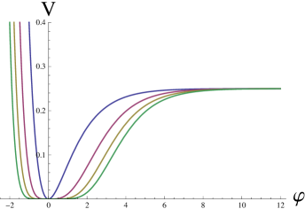
Figure 2: Models of conformal inflation based on generalizations of the Starobinsky model, with $F({\phi/\chi})\sim{\phi^{2n}\over\chi^{2n-2}(\phi+\chi)^{2}}$, $n=1,2,3,4$.

4 Universality of conformal inflation

In this section we will describe the roots of the universality of predictions of conformal inflation in a more general way. But first of all, we will consider some instructive examples, which will help to explain the main idea of our approach.

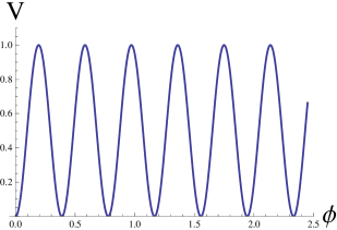
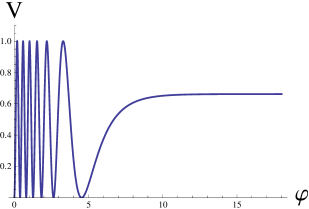
Figure 3: Flattening of the sinusoidal potential $V(\phi)$ near the boundary of the moduli space $\phi=\sqrt{6}$ by boost in the moduli space, $V(\phi)\to V(\sqrt{6}\,\tanh{\varphi\over\sqrt{6}})$. Inflationary plateau of the function $V(\phi)$ appears because of the exponential stretching of the last growing part of the sinusoidal function $V(\phi)$.

Consider a sinusoidal function $F\left({\phi/\chi}\right)\sim\sin(a+b\phi)$ and check what will happen to it after the boost $V(\phi)\to V(\sqrt{6}\,\tanh{\varphi\over\sqrt{6}})$. As we see from the Fig. 3, the main part of the stretch of the potential occurs very close to the boundary of moduli space, near $\phi=\sqrt{6}$. The rising segment of the sinusoidal function bends and forms a plateau, which has an ideal form for the slow-roll inflation. However, if the last segment of the sinusoidal function were falling down, its stretching would produce an exponentially decreasing curve rapidly approaching dS space. This possibility does not lead to slow roll inflation ending in a nearly Minkowski space in which we live now. Thus if we consider such functions, we have a 50% chance that their stretching will produce a nice inflationary potential.

Now let us study a more general and complicated potential on the full interval $-\sqrt{6}<\phi<\sqrt{6}$, as shown in Fig. 4. It shows the same effect as the one discussed above: The part of the landscape at $|\phi|\ll\sqrt{6}$ does not experience any stretching. The part with a falling field $\phi$ near the left boundary of the moduli space at $\phi=-\sqrt{6}$ becomes $dS$ or (as in Fig. 4) AdS space. The inflationary plateau appears because of the exponential stretching of the growing branch of $V(\phi)$ near $\phi=\sqrt{6}$.

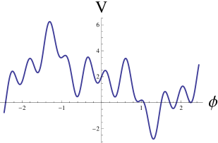
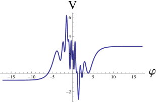
Figure 4: Flattening of a generic potential near the boundary of the moduli space by boost in the moduli space $V(\phi)\to V(\sqrt{6}\,\tanh{\varphi\over\sqrt{6}})$. In essence, what we see is ‘inflation of the inflationary landscape’ at the boundary of the moduli space, which solves the flatness problem of the inflationary potential required for inflation in the landscape.

In this scenario, inflationary regime emerges each time when $V(\phi)$ grows at the boundary of the moduli space, which is a rather generic possibility, requiring no exponential fine-tuning.

To specify the conditions required for this scenario to work, as well as its observational consequences, we will represent the potential $V(\phi)$ by expanding it in Taylor series near the boundary of the moduli space, in terms of the deviation $x$ of the field $\phi$ from $\sqrt{6}$:

$$x=1-{\phi\over\sqrt{6}}=\left(1-\tanh{\varphi\over\sqrt{6}}\right)\approx 2\ e^{-\sqrt{2/3}\,\varphi}\ ,$$ (4.1)

$$V(\varphi)=V_{*}\ (1-\sum c_{n}x^{n})=V_{*}\ \left[1-\sum c_{n}\left(2\ e^{-\sqrt{2/3}\,\varphi}\right)^{n}\right]\ ,$$ (4.2)

where $V_{*}\equiv V(x=0)$, which is equal to the asymptotic value of $V(\varphi)$ at $\varphi\to\infty$. We will try to solve this equation keeping the first term in the expansion,

$$V(\varphi)=V_{*}\ \left(1-2\,c_{1}\ e^{-\sqrt{2/3}\,\varphi}\right)\ ,$$ (4.3)

assuming that $2\,c_{1}\ e^{-\sqrt{2/3}\,\varphi}\ll 1$, and then we will estimate the contribution of higher terms.

In this approximation, equation for the field $\varphi$ in the slow roll approximation is the same as in eq. (3.5), with an obvious replacement $4n\to 2\,c_{1}$. For large $N$, this leads to relation

$$2\,c_{1}\,e^{-\sqrt{2/3}\,\varphi(N)}={3\over 2\,N}\ ,$$ (4.4)

where $\varphi_{N}$ is the value of the inflaton field at the time corresponding to $N$ e-foldings from the end of inflation.

This implies that

$$\Delta V=V_{*}-V(\varphi_{N})={3\over 2\,N}\ ,$$ (4.5)

independently of $c_{1}$, see Fig. 1. More importantly, it implies that expansion in powers of $x$ in (4.2) is, in fact, expansion in $1/N$. Therefore, unless the slope of the potential $c_{1}$ is anomalously small, or some of the coefficients $c_{n}$ are anomalously large, one can indeed ignore all higher corrections for $N\gg 1$, and all models with these properties (and $c_{1}>0$) will have identical values of $n_{s}$ and $r$, independently of the detailed structure of the model. This is the main reason for the universality which we found in many models of conformal inflation described above.

Flattening of the potentials that we have found is similar but different from the corresponding effect in the theory $\lambda\phi^{4}-{\xi\over 2}\phi^{2}R$ with $\xi>0$ [11], [12]. However, for $\xi>0$ this effect is efficient only for theories $\sim\phi^{4}$, whereas in our case the effect is more universal. The results of our approach can be further extended, for example, to the description of models with arbitrary value of $\xi<0$, see e.g. a discussion of one of such models in [15]. The main reason for flattening of the inflationary potential in the models discussed in this paper can be explained as follows.

In the original conformally invariant theory, the only conformally invariant measure of the amplitude of the scalar field $\phi$ is the ratio $z={\phi\over\chi}$. After fixing $\chi=\sqrt{6}$, which brings us to the Jordan frame, the variable $z={\phi\over\chi}$ becomes ${\phi\over\sqrt{6}}$. One can use the variable $x=1-z=1-{\phi\over\sqrt{6}}$, which we introduced in the previous section as a measure of the distance from the boundary of the moduli space at $\phi=\sqrt{6}$.

Gradients of the potential $V$ in terms of the canonically normalized field $\varphi$ are related to gradients in terms of $x$:

$$V_{\varphi}={dV\over d\varphi}={dV\over dx}{dx\over d\varphi}=\sqrt{2\over 3}\,x\,{dV\over dx}={dV\over dx}\times 2\ \sqrt{2\over 3}\ e^{-\sqrt{2/3}\,\varphi}\ ,$$ (4.6)

see eq. (4.1).

This result shows that the flatness of the potential $V(\varphi)$ (the smallness of ${dV\over d\varphi}$) can be interpreted as a result of the stretching of the moduli space, which occurs when one goes from variables $z$, $x$ or $\phi$ to the canonically normalized field $\varphi$ in the Einstein frame. At small $x$ (large $\varphi$), one has

$$d\varphi={1\over 2}\,\sqrt{3\over 2}\,e^{\sqrt{2/3}\,\varphi}\ dx\ .$$ (4.7)

Thus, any small step by $dx$ in the original conformal variables near the boundary of the moduli space translates into an exponentially longer step ${1\over 2}\sqrt{3\over 2}e^{\sqrt{2/3}\varphi}$ in terms of $\varphi$. This effect is responsible for the flattening of the inflationary potential in terms of the canonical field $\varphi$. It is reminiscent of two different effects from other areas of physics: Exponential stretching of inhomogeneities and decrease of their gradients during inflation, and redshift of light (increase of its wavelength) emitted by an observer falling towards the black hole horizon.

From these results, one can derive an additional universal parameter, the energy scale of inflation, $V\approx V_{*}$, which takes the same value for all models described above, in the leading order in $1/N$. Planck2013 data imply the following normalization of the amplitude of scalar perturbations of metric [4]:

$${V^{3}\over 12\pi^{2}V^{2}_{\varphi}}\approx 2.2\times 10^{-9}\ ,$$ (4.8)

where $V_{\varphi}={dV\over d\varphi}$. In our case, $V(\varphi_{N})=V_{*}-{3\over 2\,N}\approx V_{*}$, and

$$V_{\varphi}=V_{*}\times 2\ c_{1}\,\sqrt{2\over 3}\ e^{-\sqrt{2/3}\,\varphi}={3V_{*}\over 2\,N}\ .$$ (4.9)

This yields

$$V(\varphi_{N})=3.9\times 10^{-7}N^{-2}\sim 1.1\times 10^{-10}$$ (4.10)

in Planck units, for all models in this universality class.

5 Superconformal Universality Class Models

The superconformal action in general is defined by an embedding Kähler  potential ${\cal N}$ and superpotential ${\cal W}$, in notation of [5]

$${1\over\sqrt{-g}}\mathcal{L}_{\rm sc}^{\rm scalar-grav}=-{\textstyle\frac{1}{6}}{\cal N}(X,\bar{X})R-G_{I\bar{J}}{\cal D}^{\mu}X^{I}\,{\cal D}_{\mu}\bar{X}^{\bar{J}}-G^{I\bar{J}}{\cal W}_{I}\bar{{\cal W}}_{\bar{J}}\,,\qquad I,\bar{I}=0,1,2.$$ (5.1)

Here $X^{0}$ is a conformon, $X^{1}\equiv\Phi$ is an inflaton and $X^{3}\equiv S$ is a Goldstino, see for example [1] where this setting for our superconformal models is explained in details. The bosonic universality class models described above has an underlying class of superconformal models: the embedding Kähler  potential for these models has an $SU(1,1)$ symmetry between the complex conformon $X^{0}$ and the complex inflaton $X^{1}$ superfields.

$$\mathcal{N}(X,\bar{X})=-|X^{0}|^{2}+|X^{1}|^{2}+|S|^{2}-3\zeta\,{(S\bar{S})^{2}\over|X^{0}|^{2}-|X^{1}|^{2}}\,\,.$$ (5.2)

We take the superpotential which preserves a subgroup of $SU(1,1)$, namely an $SO(1,1)$, which makes a boost between the holomorphic parts of $X^{0}$ and $X^{1}$.

$${\cal W}=S\Big{(}(X^{0})^{2}-(X^{1})^{2}\Big{)}f(X^{1}/X^{0})\ .$$ (5.3)

Function $f(X^{1}/X^{0})$ is invariant under local conformal-$\mathbb{R}$-symmetry, but if it is not a constant, it breaks the $SO(1,1)$.

5.1 Conformal-$\mathbb{R}$-symmetry gauge $X^{0}=\bar{X}^{0}=\sqrt{3}$

In the gauge where we fix the local conformal as well as a local $U(1)$ symmetry by taking $X^{0}=\bar{X}^{0}=\sqrt{3}$ and with $X^{1}\equiv\Phi$ we recover, following [6, 7], a supergravity version of the superconformal model with

$$K=-3\ln\Big{[}1-{|\Phi|^{2}+|S^{2}|\over 3}+\zeta\,{(S\bar{S})^{2}\over 3-|\Phi|^{2}}\Big{]},$$ (5.4)

and

$$W=S\Big{(}3-(\Phi)^{2}\Big{)}f(\Phi/\sqrt{3})\ .$$ (5.5)

An advantage of this gauge is that we may use a well tested over the years Mathematica code [23], developed further in [24], and study moduli stabilization. In this case the inflaton is a real part of $\Phi$. In particular at $S=0$ our condition that $1-{|\Phi|^{2}|\over 3}>0$ is a condition that we are inside a ‘Kähler  cone’. The kinetic term for the scalar $\Phi$ is

$$\Big{(}{1\over 1-|\Phi|^{2}/3}\Big{)}^{2}\partial_{\mu}\Phi\partial^{\mu}\bar{\Phi}\ .$$ (5.6)

The positivity of the kinetic term for scalars requires that $|\Phi|^{2}<3$. The boundary of the moduli space here is a ‘Kähler  cone’

$$1-{|\Phi^{2}|\over 3}=0\ .$$ (5.7)

We find that the condition for stability of goldstino at $S=0$ for all values of the inflaton is provided by $\zeta>1/6$ in (5.4). Inflation is stable at $\rm Im\Phi=0$ independently of the value of $\zeta$.

As an example of a theory with all moduli stabilized, we show the potential of the fields $\varphi$ and $S$ in the supergravity generalization of the T-Model with $\zeta=1$ in Fig. 5.

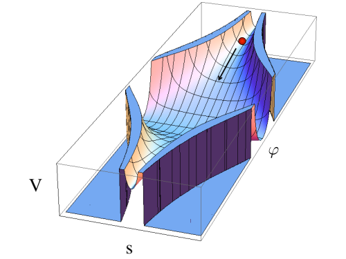
Figure 5: Supergravity version of the T-Model. The $S$-direction is steep, the system quickly reaches the minimum at $S=0$ and evolves in the inflaton direction $\varphi$ at stabilized $S$.

5.2 $SO(1,1)$ invariant conformal-$\mathbb{R}$-symmetry rapidity gauge $(X^{0})^{2}-(X^{1})^{2}=3$

Now we use the fact which we learned from the previous subsection, using Mathematica: inflation takes place at

$$S=0\,,\qquad X^{1}=\bar{X}^{1}=\varphi/\sqrt{2}\ .$$ (5.8)

In this gauge we may resolve the $SO(1.1)$ constraint so that

$$X^{0}=\sqrt{3}\cosh\varphi/\sqrt{6}\ ,\qquad X^{1}=\sqrt{3}\sinh\varphi/\sqrt{6}\ .$$ (5.9)

The superconformal action (5.1) with (5.2) and (5.3) entries becomes at $S=0$, $X^{1}=\bar{X}^{1}=\varphi/\sqrt{2}$

$${1\over\sqrt{-g}}\mathcal{L}_{\rm sc}^{\rm scalar-grav}={\textstyle\frac{1}{2}}R-{1\over 2}(\partial^{\mu}\varphi)^{2}-|f(\tanh\varphi)|^{2}\,.$$ (5.10)

This shows the origin of the bosonic universality class models in case that $F=f\bar{f}$.

6 Emergence of (super)conformal critical phenomena in cosmology

Numerous studies of supersymmetric attractors in general relativity so far focused on black hole type geometries, where stabilization of moduli near the black holes horizon was described as a critical phenomena, starting with [25] where it was shown that supersymmetric attractors have certain universality classes.

The superconformal critical phenomena in cosmology were already introduced in [1]. It was observed there that the model ${\lambda\over 4}\phi^{4}-{\xi\over 2}\phi^{2}R$, when embedded into a corresponding superconformal theory, provides an interpretation of the non-minimal coupling parameter $\xi$ as a deviation from the critical point $\xi=0$. In the superconformal model the relevant parameter $\Delta$ represents a deviation of the embedding Kähler  manifold from the flat one. This parameter has one critical point $\Delta_{\rm cr}=0$ corresponding to the $SU(1,1)$ symmetry between the inflaton $X^{1}$ multiplet and the conformon $X^{0}$ multiplet. It has another double critical point $\Delta_{\rm cr}=\pm 1/6$ corresponding to an enhanced symmetry between the inflaton and the conformon. At this critical point the parameter of the non-minimal coupling to gravity in the bosonic models becomes equal to the difference of the parameter $\Delta$ from the critical point $\Delta_{\rm cr}=\pm 1/6$, i. e. $\xi=\Delta-\Delta_{\rm cr}$. This allows to interpret $\xi\geq 2\cdot 10^{-3}$ as a deviation of $\Delta$ from the superconformal critical point $\Delta_{\rm cr}=\pm 1/6$ to fit the Planck data [4]. Note that without the conformal embedding there is no meaning for the parameter $\xi=0$ as a critical point, a point of enhanced symmetry. In presence of the conformon, which is required for the conformal symmetry of the action, the critical points and the corresponding critical phenomena in cosmology can be clearly formulated and studied.

In this paper, the critical phenomena are described with regard to a critical value $\Delta_{\rm cr}=0$, when the embedding Kähler  manifold remains flat and preserves an $SU(1,1)$ symmetry. This symmetry is broken to the $SO(1,1)$ symmetry by the superpotential. The critical point in this case is de Sitter space. The deviation from the critical point is introduced via an arbitrary zero conformal weight function $f(z)$ of the homogeneous coordinate $z=X^{1}/X^{0}$ in the superpotential. Under Weyl symmetry and $U(1)$ $\mathbb{R}$-symmetry $z$ is invariant, therefore an arbitrary function $f(z)$ is the only way to describe the deformation of the model near the critical point with $SO(1,1)$ symmetry preserving the local superconformal symmetry of the action. As expected from the general theory of critical phenomena, we find a universality class for such models. What was not known, a priory, is that the attractor point for this universality class models is in fact the one given in eq. (1.1).

7 Conclusions

We described the emergence of the critical phenomena which arise in the framework of the superconformal approach to cosmology [5]. This approach helps to classify and generalize a certain class of models favored by Planck. In this paper as well as in [1, 2] we have shown that the data may be associated with attractor points in the $n_{s}$-$r$ plane where there a universality class of models with the same (favored by Planck) values of $n_{s}$ and $r$ (1.1) and inflationary energy density (4.10).

In the context of this approach we identified the effect of exponential flattening of the potentials which appear in a large class of conformal and superconformal models. In these models, the original inflationary potential should be specified in terms of homogeneous coordinates $z$ that are invariant with respect to (super)conformal transformations. For example, for the conformal theory of the conformon $\chi$ and inflaton $\phi$, this variable is $z=\phi/\chi$. After the gauge fixing and converting into the Einstein frame, the finite interval of variation of $z$ is stretched into an infinite range of the canonical field $\varphi$, which is similar to rapidity in the special theory of relativity. This stretching is similar to inflation which leads to exponential suppression of gradients of inhomogeneities in inflationary universe. In our context, this stretching leads to exponential flattening of the potentials $V(z)$ of the original conformal or superconformal theory, expressed in terms of the canonical field $\varphi$ describing these potentials in the Einstein frame. This effect facilitates inflation in the theories with a broad class of potentials $V(z)$ and leads to universality of their observational predictions.

It is likely that other interesting developments in inflationary cosmology along the lines developed in [1, 2] and in this paper will follow, and new attractor points in the evolution of the universe will be discovered.

Acknowledgments

Our work was influenced by discussions with G. ‘t Hooft about the opportunities to understand physics via spontaneous breaking / alternative gauge-fixing of conformal symmetry. We are grateful to R. Bond, G. Horowitz, V. Mukhanov, E. Silverstein, M. Srednicki, L. Susskind, and participants of the Primordial Cosmology workshop in KITP for stimulating discussions. This work is supported by the SITP and by the NSF Grant No. 0756174, the work of RK is also supported by the Templeton Foundation Grant “Frontiers of Quantum Gravity”.

8 Appendix: ‘Special relativity’ in the moduli space: rapidity versus velocity

The mechanism of flattening the inflationary potentials described in our paper is related to approach to a vicinity of a critical point of a system at the boundary of the moduli space. It is geometric and universal for a large class of models. The physical reason for this phenomena is as deep as the fact that the speed of light $c=1$ cannot be exceeded. At small velocities the addition rule is

$$v=v_{1}+v_{2}\ .$$ (8.1)

Meanwhile, at large velocities the rule is such that

$$v={v_{1}+v_{2}\over 1+v_{1}v_{2}}\ ,$$ (8.2)

so that it never exceeds speed of light. Meanwhile, if we describe the motion using rapidity, instead, the addition rule is

$$\tanh\theta={\tanh\theta_{1}+\tanh\theta_{2}\over 1+\tanh\theta_{1}\tanh\theta_{2}}=\tanh(\theta_{1}+\theta_{2})\ .$$ (8.3)

This means that rapidities have a simple addition rule,

$$\theta=\theta_{1}+\theta_{2}\ .$$ (8.4)

meanwhile it is guaranteed that $\tanh$ of any argument never exceeds 1 and speed of light remains the maximal possible velocity.

At small velocities

$$\tanh\theta\approx\theta\,,\qquad(\tanh\theta)^{2n}\approx\theta^{2n}\ .$$ (8.5)

However, at large $\theta$ the situation changes dramatically:

$$(\tanh\theta)^{2n}|_{\theta\rightarrow\infty}\Rightarrow 1\,,\qquad\theta^{2n}|_{\theta\rightarrow\infty}\Rightarrow\infty\ .$$ (8.6)

This is what we find in our potentials, up to the obvious replacement $\theta\to\varphi/\sqrt{6}$, see for example T-Model in Fig. 1. The potential at small $\varphi$ may be more or less steep, it does not matter, they all approach an attractor point at large $\varphi$, independently of their initial steepness: they comply with ‘special relativity’ in the moduli space. The major property of the attractor system is that in the process of evolution the system develops to a common final point, independently of initial conditions.

References

- [1] R. Kallosh and A. Linde, “Superconformal generalization of the chaotic inflation model ,” JCAP 1306, 027 (2013) [arXiv:1306.3211 [hep-th]].
- [2] R. Kallosh and A. Linde, “Superconformal generalizations of the Starobinsky model,” JCAP 1306, 028 (2013) [arXiv:1306.3214 [hep-th]].
- [3] G. Hinshaw et al. [WMAP Collaboration], “Nine-Year Wilkinson Microwave Anisotropy Probe (WMAP) Observations: Cosmological Parameter Results,” arXiv:1212.5226 [astro-ph.CO].
- [4] P. A. R. Ade et al. [ Planck Collaboration], “Planck 2013 results. XXII. Constraints on inflation,” arXiv:1303.5082 [astro-ph.CO]. P. A. R. Ade et al. [Planck Collaboration], “Planck 2013 results. XVI. Cosmological parameters,” arXiv:1303.5076 [astro-ph.CO].
- [5] R. Kallosh, L. Kofman, A. D. Linde and A. Van Proeyen, “Superconformal symmetry, supergravity and cosmology,” Class. Quant. Grav. 17, 4269 (2000) [Erratum-ibid. 21, 5017 (2004)] [arXiv:hep-th/0006179].
- [6] S. Ferrara, R. Kallosh, A. Linde, A. Marrani and A. Van Proeyen, “Jordan Frame Supergravity and Inflation in NMSSM,” Phys. Rev. D82, 045003 (2010) [arXiv:1004.0712 [hep-th]].
- [7] S. Ferrara, R. Kallosh, A. Linde, A. Marrani, A. Van Proeyen and , “Superconformal Symmetry, NMSSM, and Inflation,” Phys. Rev. D 83, 025008 (2011) [arXiv:1008.2942 [hep-th]].
- [8] A. A. Starobinsky, “A New Type of Isotropic Cosmological Models Without Singularity,” Phys. Lett. B 91, 99 (1980). A. A. Starobinsky, “The Perturbation Spectrum Evolving from a Nonsingular Initially De-Sitter Cosmology and the Microwave Background Anisotropy,” Sov. Astron. Lett. 9, 302 (1983).
- [9] V. F. Mukhanov and G. V. Chibisov, “Quantum Fluctuation and Nonsingular Universe. (In Russian),” JETP Lett. 33, 532 (1981) [Pisma Zh. Eksp. Teor. Fiz. 33, 549 (1981)]. V.F. Mukhanov, “Physical Foundations of Cosmology” (Cambridge University Press, 2005).
- [10] A. D. Linde, “Chaotic Inflation,” Phys. Lett. B 129, 177 (1983).
- [11] D. S. Salopek, J. R. Bond and J. M. Bardeen, Designing density fluctuation spectra in inflation, Phys. Rev. D40, 1753 (1989).
- [12] F. L. Bezrukov and M. Shaposhnikov, “The Standard Model Higgs boson as the inflaton,” Phys. Lett. B 659, 703 (2008) [arXiv:0710.3755 [hep-th]]. F. Bezrukov, D. Gorbunov and M. Shaposhnikov, “On initial conditions for the Hot Big Bang,” JCAP 0906, 029 (2009) [arXiv:0812.3622 [hep-ph]]. J. Garcia-Bellido, D. G. Figueroa and J. Rubio, “Preheating in the Standard Model with the Higgs-Inflaton coupled to gravity,” Phys. Rev. D 79, 063531 (2009) [arXiv:0812.4624 [hep-ph]]. A. De Simone, M. P. Hertzberg and F. Wilczek, “Running Inflation in the Standard Model,” Phys. Lett. B 678, 1 (2009) [arXiv:0812.4946 [hep-ph]]. F. Bezrukov and M. Shaposhnikov, “Standard Model Higgs boson mass from inflation: two loop analysis,” JHEP 0907, 089 (2009) [arXiv:0904.1537 [hep-ph]]. A. O. Barvinsky, A. Y. Kamenshchik, C. Kiefer, A. A. Starobinsky and C. Steinwachs, “Asymptotic freedom in inflationary cosmology with a non-minimally coupled Higgs field,” JCAP 0912, 003 (2009) [arXiv:0904.1698 [hep-ph]]. G. F. Giudice and H. M. Lee, “Unitarizing Higgs Inflation,” Phys. Lett. B 694, 294 (2011) [arXiv:1010.1417 [hep-ph]]. N. Okada, M. U. Rehman, Q. Shafi and , “Tensor to Scalar Ratio in Non-Minimal Inflation,” Phys. Rev. D 82, 043502 (2010) [arXiv:1005.5161 [hep-ph]]. F. Bezrukov and D. Gorbunov, “Light inflaton after LHC8 and WMAP9 results,” arXiv:1303.4395 [hep-ph].
- [13] M. B. Einhorn and D. R. T. Jones, “Inflation with Non-minimal Gravitational Couplings in Supergravity,” JHEP 1003, 026 (2010) [arXiv:0912.2718 [hep-ph]].
- [14] H. M. Lee, “Chaotic inflation in Jordan frame supergravity,” JCAP 1008, 003 (2010) [arXiv:1005.2735 [hep-ph]].
- [15] A. Linde, M. Noorbala and A. Westphal, “Observational consequences of chaotic inflation with nonminimal coupling to gravity,” JCAP 1103, 013 (2011) [arXiv:1101.2652 [hep-th]].
- [16] J. Ellis, D. V. Nanopoulos and K. A. Olive, “A No-Scale Supergravity Realization of the Starobinsky Model,” arXiv:1305.1247 [hep-th].
- [17] W. Buchmuller, V. Domcke and K. Kamada, “The Starobinsky Model from Superconformal D-Term Inflation,” arXiv:1306.3471 [hep-th].
- [18] X. Dong, B. Horn, E. Silverstein and A. Westphal, “Simple exercises to flatten your potential,” Phys. Rev. D 84, 026011 (2011) [arXiv:1011.4521 [hep-th]].
- [19] A. B. Goncharov and A. D. Linde, “Chaotic Inflation In Supergravity,” Phys. Lett. B 139, 27 (1984).
- [20] A. D. Linde, “Chaotic Inflation With Constrained Fields,” Phys. Lett. B 202, 194 (1988). A. D. Linde, “Creation of a compact topologically nontrivial inflationary universe,” JCAP 0410, 004 (2004) [hep-th/0408164]. A. D. Linde, “Inflationary Cosmology,” Lect. Notes Phys. 738, 1 (2008) [arXiv:0705.0164 [hep-th]].
- [21] A. D. Linde, “The Inflationary Universe,” Rept. Prog. Phys. 47, 925 (1984). A. D. Sakharov, “Cosmological Transitions With A Change In Metric Signature,” Sov. Phys. JETP 60, 214 (1984) [Zh. Eksp. Teor. Fiz. 87, 375 (1984)]. T. Banks, “T C P, Quantum Gravity, the Cosmological Constant and All That…,” Nucl. Phys. B 249, 332 (1985). J. D. Barrow, F. J. Tipler. The Anthropic Cosmological Principle (Oxford University Press, NY, 1986). A. D. Linde, “Inflation and quantum Cosmology,” Print-86-0888, 1 July 1986 (published in: 300 Years of Gravitation, Eds. S. W. Hawking and W. Israel, Cambridge University Press, Cambridge, 1987). S. Weinberg, “Anthropic Bound on the Cosmological Constant,” Phys. Rev. Lett. 59, 2607 (1987). G. Efstathiou, MNRAS 274, L73 (1995). H. Martel, P. R. Shapiro and S. Weinberg, “Likely values of the cosmological constant,” Astrophys. J. 492, 29 (1998) [astro-ph/9701099]. J. Garriga, M. Livio and A. Vilenkin, “The Cosmological constant and the time of its dominance,” Phys. Rev. D 61, 023503 (2000) [astro-ph/9906210].
- [22] R. Bousso and J. Polchinski, “Quantization of four form fluxes and dynamical neutralization of the cosmological constant,” JHEP 0006, 006 (2000) [hep-th/0004134]. S. Kachru, R. Kallosh, A. D. Linde and S. P. Trivedi, “De Sitter vacua in string theory,” Phys. Rev. D 68, 046005 (2003) [hep-th/0301240]. M. R. Douglas, “The Statistics of string / M theory vacua,” JHEP 0305, 046 (2003) [hep-th/0303194]. L. Susskind, “The Anthropic landscape of string theory,” In *Carr, Bernard (ed.): Universe or multiverse?* 247-266 [hep-th/0302219].
- [23] R. Kallosh and S. Prokushkin, “SuperCosmology,” hep-th/0403060.
- [24] R. Kallosh, A. Linde, “New models of chaotic inflation in supergravity,” JCAP 1011, 011 (2010) [arXiv:1008.3375 [hep-th]]. R. Kallosh, A. Linde, T. Rube, “General inflaton potentials in supergravity,” Phys. Rev. D 83, 043507 (2011) [arXiv:1011.5945 [hep-th]].
- [25] S. Ferrara, R. Kallosh and A. Strominger, “N=2 extremal black holes,” Phys. Rev. D 52, 5412 (1995) [hep-th/9508072]. S. Ferrara and R. Kallosh, “Supersymmetry and attractors,” Phys. Rev. D 54, 1514 (1996) [hep-th/9602136]. S. Ferrara and R. Kallosh, “Universality of supersymmetric attractors,” Phys. Rev. D 54, 1525 (1996) [hep-th/9603090].