Modification to Darcy model for high pressure and high velocity applications and associated mixed finite element formulations

Abstract.

The Darcy model is based on a plethora of assumptions. One of the most important assumptions is that the Darcy model assumes the drag coefficient to be constant. However, there is irrefutable experimental evidence that viscosities of organic liquids and carbon-dioxide depend on the pressure. Experiments have also shown that the drag varies nonlinearly with respect to the velocity at high flow rates. In important technological applications like enhanced oil recovery and geological carbon-dioxide sequestration, one encounters both high pressures and high flow rates. It should be emphasized that flow characteristics and pressure variation under varying drag are both quantitatively and qualitatively different from that of constant drag. Motivated by experimental evidence, we consider the drag coefficient to depend on both the pressure and velocity. We consider two major modifications to the Darcy model based on the Barus formula and Forchheimer approximation. The proposed modifications to the Darcy model result in nonlinear partial differential equations, which are not amenable to analytical solutions. To this end, we present mixed finite element formulations based on least-squares (LS) formalism and variational multi-scale (VMS) formalism for the resulting governing equations. The proposed modifications to the Darcy model and its associated finite element formulations are used to solve realistic problems with relevance to enhanced oil recovery. We also study the competition between the nonlinear dependence of drag on the velocity and the dependence of viscosity on the pressure. To the best of the authors’ knowledge such a systematic study has not been performed.

1. INTRODUCTION AND MOTIVATION

Understanding the flow of fluids through porous media plays a crucial role in various technological applications (e.g., designing filters, enhanced oil recovery, geological carbon-dioxide sequestration) and for mathematical modeling in various branches of engineering (e.g., civil engineering, petroleum engineering, polymer engineering). Arguably, the most popular model in the studies on flow through porous media is the Darcy model, which is named after the French hydraulics engineer Henry Darcy who first proposed the equation in 1856 [1]. Darcy originally developed the model empirically based on the experiments on the flow of water in sand beds. However, the Darcy model can be given firm mathematical basis at least in two different ways. One approach is by applying the volume averaging theory on the Navier-Stokes equations [2]. The other approach is using the theory of interacting continua (also known as mixture theory). For example, see reference [3, Introduction]). In this paper, the latter approach will be employed.

1.1. Limitations of Darcy model, and its generalizations

Darcy equations model the flow of an incompressible fluid in rigid porous media by stating that the (Darcy) velocity is linearly proportional to the gradient of the pressure. It is important to note that the Darcy equation is simply an approximation of the balance of linear momentum in the context of theory of interacting continua. It merely predicts the flux but cannot predict stresses in solids. That is, this model cannot be used with modification when there is deformation / damage of the porous solid (e.g., in the case of hydraulic fracture). For completeness and future reference, let us enumerate the key assumptions behind the Darcy model [3]. $\bullet$ There is no mass production of individual constituents (i.e., there are no chemical reactions). $\bullet$ The porous solid is assumed to be rigid. Thus, the balance laws for the solid are trivially satisfied. In particular, the stresses in the solid are what they need to be to ensure that the balance of linear momentum is met. $\bullet$ The fluid is assumed to be homogeneous and incompressible. $\bullet$ The velocity and its gradient are assumed to be small so that the inertial effects can be ignored. $\bullet$ The partial stress in the fluid is that of an Euler fluid. That is, there is no dissipation of energy between fluid layers. $\bullet$ The only interaction force is at the fluid and pore boundaries. $\bullet$ Darcy model assumes that the drag coefficient is independent of the pressure and the velocity. Experimental studies have shown that the viscosity of organic liquids (and hence the drag coefficient) depend on the pressure [4, 5] and the drag coefficient depends on the velocity at high velocities [6, 7]. Therefore, Darcy model as it is not appropriate for applications involving high pressure and high flow velocities. Application of Darcy model in such situations can result in erroneous predictions of discharge fluxes and inaccurate pressure contours. While several generalizations of the standard Darcy model have been proposed in the literature, none of these studies addressed the study undertaken in this paper. In particular, the prior studies did not address the combined effect of pressure-dependent viscosity and the dependence of drag coefficient on the velocity.

1.1.1. Enhanced oil recovery

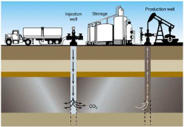
Figure 1. A pictorial description of enhanced oil recovery. [Source: https://www.llnl.gov/str/November01/Kirkendall.html]

Over the years people have used Darcy model beyond its range of applicability. One example of misuse is in the modeling enhanced oil recovery (EOR) applications. As illustrated in Figure 1, steam / carbon-dioxide gas is injected into the ground through injection wells. The gas create a pressure build up in the ground (i.e., the porous media) and pushes the fluid (i.e., raw oil) out through the production wells. High pressures ranging from $10-100\;\mathrm{MPa}$ are employed, and such high pressures can lead to inaccurate flow estimates or pressure contours if the original Darcy model is used. Oil reservoir simulations are tricky by nature because of the possibility of having varying permeability within layers, impervious zones, non-rigid rock and soil formations, and pockets of natural gases. Seismic imaging and field experimentation may not always return the most accurate data so one must be extremely cautious when providing parameters to run numerical models. Using the right Darcy modification(s) allows one to predict more accurate production rates, help industries determine where to allocate their resources, and prevent environmental damage from unintended cracking in the subsurface.

1.2. Mixed formulations

For the proposed model, we present mixed finite element formulations based on two different approaches: least-squares (LS) finite element method [8] and variational multi-scale (VMS) formalism [9]. It is well-known that care should be taken when working with mixed formulations. In order to get stable results, a mixed formulation should either satisfy or circumvent the Ladyzhenskaya-Babuška-Brezzi (LBB) stability condition [10]. Both the proposed mixed formulations proposed in this paper circumvent the LBB condition.

The least-squares finite element method (LSFEM) is based on the minimization of the residuals in a least-squares sense. One can always obtain a symmetric positive definite system of algebraic equations, even for non-self-adjoint problems. The LSFEM provides greater accuracy for the derivatives of primal variables when compared to single-field formulations, boundary conditions are easy to manage, the conformity of finite element spaces is sufficient to guarantee stability, and all variables can use the same finite element space. For further discussion on the LSFEM, see references [11, 8].

The VMS formalism adds stabilization terms to the classical mixed formulation. The stabilization terms and the stabilization parameter can be derived in a consistent manner (e.g., see references [9, 12]). A mixed formulation based on the VMS formalism falls under the category of stabilized methods, as in some sense the formulation is obtained by stabilizing the classical mixed formulation [13]. Several studies as shown in references [14, 15, 16, 17, 18] have proposed various stabilized formulations that provide accurate solutions of Darcy model through porous media, but none of these studies considered the proposed model. Some notable mixed formulation based on the VMS formalism for Darcy-type equations are references [19, 12, 3, 20]. We shall demonstrate in a subsequent section that the proposed mixed formulation encompasses these mixed formulations.

1.2.1. Local mass balance

A common drawback of finite element formulations is that they need not possess local / element-wise mass balance property. In particular, the mixed formulations from both the LS and VMS formalisms do not possess the local mass balance property. It should be noted that while it is possible to achieve local mass conservation for the LS formalism, one would no longer be able to obtain continuous nodal quantities (e.g., see reference [21]). Several independent studies [22, 23, 24] have successfully developed conservative finite element formulations for flow through porous media problems, but none of them have been extended to modifications of Darcy’s model. Another relevant work is reported in reference [25] in which the effect of error in local mass balance on the transport of chemical species is studied. This study considered coupled flow and transport problems, and the comparison is made between a VMS-based formulation and the locally mass conservative Raviart-Thomas formulation. Herein, we shall perform a systematic study on the performance of the proposed mixed formulations for various flow models with respect to the local mass balance property. This study is intended to serve two purposes. First, it will guide users of the finite element method (FEM) on the extent of the violation of local mass balance under mixed formulations. Second, it will encourage researchers to improve the performance of finite element formulations with respect to local balance under arbitrary interpolation functions for the velocity and pressure.

1.3. Main contributions of this paper

Several contributions have been made in this paper with respect to modeling of flow through porous media, associated mixed formulations, and numerical solutions of representative problems. Some of the main ones are as follows:

1. To propose a generalization of the Darcy model by taking into account both the dependence of viscosity on the pressure and the dependence of drag coefficient on the velocity. The classical Darcy-Forchheimer and the modified Darcy model that is considered in reference [3] will be special cases of the generalized model considered in this paper. The generalization is referred to as the modified Darcy-Forchheimer model.

2. To present some theoretical results pertaining to the modified Darcy-Forchheimer model, and demonstrate their utility in validating numerical implementations.

3. To develop a mixed formulation based on LS formalism for the modified Darcy-Forchheimer model and study the effect of weighting on the convergence and accuracy of the solutions.

4. To construct a mixed formulation based on the VMS formalism for the modified Darcy-Forchheimer model, which encompasses as special cases some of the existing mixed formulations proposed for simpler models.

5. To compare the numerical performances of VMS and LS based mixed formulations.

6. To document the local mass balance error under both these formalisms for the standard Darcy model and for its generalizations.

7. It has been claimed in references [12, 26] that VMS formulation is the only known mixed formulation that satisfies three-dimensional constant patch test under non-constant Jacobian finite elements for the standard Darcy model. Herein, we show that the proposed LS based formulation (which is different from the variational formulation proposed in these references) also satisfies three-dimensional constant flow patch tests.

8. To discuss the implications and applicability of these modified models in numerical simulations of enhanced oil recovery. It will also be show that the pressure profiles of Darcy-Forchheimer are qualitatively and quantitatively different from that of a modification of Darcy model that takes into account the dependence of viscosity on the pressure.

9. To illustrate an important competing effect due to the dependence of viscosity on the pressure and the dependence of drag coefficient on the velocity. Specifically, to show the dependence of drag coefficient on the velocity will create steep gradients in the pressure near the projection well. On the other hand, the dependence of viscosity on the pressure creates steep pressure gradients near the injection wells. However, both these effects give rise to ceiling flux.

1.4. Organization of the paper

The remainder of the paper is organized as follows. In Section 2 modifications to Darcy model using Barus formula and Forchheimer terms are presented. In Section 3, mixed finite element formulations based on LS and VMS formalisms are proposed. In Section 4, several representative test problems are solved to show the performance and convergence of the proposed mixed finite element formulations, and to illustrate the predictive capabilities of the modified Darcy-Forchheimer model. In Section 5, several representative problems with relevance to enhanced oil recovery are simulated, and the numerical solutions from the various models and formalisms are compared. Conclusions are drawn in Section 6.

2. GOVERNING EQUATIONS: DARCY MODEL AND ITS GENERALIZATION

Let $\Omega\subset\mathbb{R}^{nd}$ be an open and bounded set, where “$nd$” denotes the number of spatial dimensions. Let $\partial\Omega:=\mathrm{cl}(\Omega)-\Omega$ be the boundary (where $\mathrm{cl}(\Omega)$ is the set closure of $\Omega$), which is assumed to be piecewise smooth. A spatial point in $\mathrm{cl}(\Omega)$ is denoted by $\mathbf{x}$. The gradient and divergence operators with respect to $\mathbf{x}$ are, respectively, denoted by $\mathrm{grad}[\cdot]$ and $\mathrm{div}[\cdot]$. Let $\mathbf{v}:\Omega\rightarrow\mathbb{R}^{nd}$ denote the “Darcy” velocity vector field (which is a homogenized velocity), and let $p:\Omega\rightarrow\mathbb{R}$ denote the pressure field. The boundary is divided into two parts, denoted by $\Gamma^{v}$ and $\Gamma^{p}$, such that $\Gamma^{v}\cap\Gamma^{p}=\emptyset$ and $\Gamma^{v}\cup\Gamma^{p}=\partial\Omega$. $\Gamma^{v}$ is the part of the boundary on which the normal component of the velocity is prescribed, and $\Gamma^{p}$ is part of the boundary on which the pressure is prescribed.

We now consider the flow of an incompressible fluid through rigid porous media based on modifications to the standard Darcy model. The governing equations take the following form:

$$\alpha(\mathbf{v},p,\mathbf{x})\mathbf{v}(\mathbf{x})+\mathrm{grad}[p(\mathbf{x})]=\rho\mathbf{b}(\mathbf{x})\quad\mathrm{in}\;\Omega$$ (1a)

$$\mathrm{div}[\mathbf{v}(\mathbf{x})]=0\quad\mathrm{in}\;\Omega$$ (1b)

$$\mathbf{v}(\mathbf{x})\cdot\mathbf{\hat{n}}(\mathbf{x})=v_{n}(\mathbf{x})\quad\mathrm{on}\;\Gamma^{v}$$ (1c)

$$p(\mathbf{x})=p_{0}(\mathbf{x})\quad\mathrm{on}\;\Gamma^{p}$$ (1d)

where $\alpha$ is the drag coefficient (which can depend on the velocity and pressure, and can spatially vary), $v_{n}(\mathbf{x})$ is the prescribed normal component of the velocity, $p_{0}(\mathbf{x})$ is the prescribed pressure, $\rho$ is the density of the fluid, $\mathbf{b}(\mathbf{x})$ is the specific body force, and $\mathbf{\hat{n}}(\mathbf{x})$ is the unit outward normal vector to the boundary. It can be shown that equation (1a) is an approximation to the balance of linear momentum under the mathematical framework offered by the theory of interacting continua (e.g., see reference [3, Introduction]). A more thorough discussion on the theory of interacting continua can be found in the several appendices of reference [27], Atkin and Craine [28], and Bowen [29].

2.1. Boundary conditions and well-posedness

We now briefly discuss the well-posedness of the aforementioned boundary value problem given by equations (1a)–(1d) in the sense of Hadamard [30]. If $\Gamma^{v}=\partial\Omega$ (i.e., the normal component of the velocity is prescribed on the entire boundary), one has to meet the following compatibility condition for well-posedness:

$$\int_{\Gamma^{v}=\partial\Omega}v_{n}(\mathbf{x})\;\mathrm{d}\Gamma=0$$ (2)

which is a direct consequence of the divergence theorem. To wit,

$$0=\int_{\Omega}\mathrm{div}[\mathbf{v}(\mathbf{x})]\;\mathrm{d}\Omega=\int_{\partial\Omega}\mathbf{v}(\mathbf{x})\cdot\hat{\mathbf{n}}(\mathbf{x})\;\mathrm{d}\Gamma=\int_{\partial\Omega}v_{n}(\mathrm{x})\;\mathrm{d}\Gamma$$ (3)

Moreover, if $\Gamma^{p}=\emptyset$ (i.e., $\partial\Omega=\Gamma^{v}$), one needs to augment the above equations (1a)–(1d) with an additional condition for uniqueness of the solution. Otherwise, one cannot find the pressure uniquely. In the Mathematics literature, the uniqueness is typically achieved by meeting the condition

$$\int_{\Omega}p(\mathbf{x})\;\mathrm{d}\Omega=0$$ (4)

which basically fixes the datum for the pressure. However, this approach is seldom used in a computational setting as it is difficult to enforce the above condition numerically. An alternative is to fix the datum for the pressure by prescribing the pressure at a point, which is commonly employed in various computational settings and is also employed in this paper.

It should also be noted that the no-slip boundary condition is not compatible with the Darcy model and the generalization that is considered in this paper. A simple mathematical explanation can be provided by noting that the inclusion of no-slip boundary condition (in addition to the no-penetration boundary condition) will make the boundary value problem over-determined. Also, it is noteworthy that the governing equations based on Darcy model are first-order (in terms of number of derivatives) with respect to the field variables $\mathbf{v}(\mathbf{x})$ and $p(\mathbf{x})$.

2.2. Darcy model, experimental evidence, and its generalization

The Darcy model assumes that the drag coefficient is independent of the pressure and velocity. In addition, the Darcy model assumes the drag coefficient to be of the form

$$\alpha=\frac{\mu}{k}$$ (5)

where $\mu$ is the coefficient of viscosity of the fluid, and $k$ is the coefficient of permeability. From the above discussion it is evident that Darcy model cannot be employed for situations in which the viscosity depends on the pressure, permeability depends on the (pore) pressure, or drag does not depend linearly on the velocity of the fluid (i.e., the drag coefficient depends on the velocity). Several experiments have shown unequivocally that these three situations occur in nature, which will now be discussed.

2.2.1. Pressure-dependent viscosity

Bridgman [4] has shown that the viscosity of several organic liquids depend on the pressure, and in fact, the dependence is exponential. Notable scientists such as Andrade [31] and Barus [5] have performed laboratory experiments on liquids to determine the relationship between pressure and viscosity. In recent years, research such as that in [32] has been able to obtain empirical evidence to delineate and confirm the dependency of viscosity on pressure. Furthermore, numerical studies have been performed in references [33, 34] to record the differences these pressure dependent viscosity equations make for several fluid problems like the Navier-Stokes equation.

There are several ways one can generalized the standard Darcy model. For example, one can model the friction between the layers of the fluid, which the standard Darcy model neglects. This is approach taken by Brinkman (see references [35, 36]). The research conducted in this paper focuses on generalizing the standard Darcy model by modifying the drag to depend on the velocity and the pressure.

To account for the dependence of the viscosity (and hence the drag) on the pressure, Barus’ formula [37]will be used. The drag coefficient based on Barus’ formula can be rewritten as

$$\alpha(p,\mathbf{x})=\frac{\mu(p)}{k(\mathbf{x})}=\frac{\mu_{0}}{k(\mathbf{x})}\exp[\beta_{\mathrm{B}}p]$$ (6)

where $\mu_{0}$ is the fixed viscosity of the fluid and $\beta_{\mathrm{B}}$ is the Barus coefficient that is obtained experimentally. This proposed modification states that the viscosity varies exponentially with pressure, and one can determine the Barus coefficient $\beta_{\mathrm{B}}$ using laboratory experiments, and its value for common organic liquids (e.g., Naphthenic mineral oil) has been documented in the literature. For example, see references [4, 38, 39, 40]).

2.2.2. High velocity flows and inertial effects

It has been experimentally observed that for high velocity flows in porous media, the flux (and hence the flow rate) is not linearly proportional to the gradient of the pressure. This can be explained by noting that inertial effects can play a dominant role for high velocity flows. The standard Darcy model completely ignores inertial effects. To address the nonlinear dependence of the flux on the gradient of the pressure for high velocity flows, Philipp Forchheimer, an Austrian scientist (1852–1933), proposed that the drag coefficient to depend on the velocity of the fluid [6]. Herein, the model that is obtained after incorporating Forchheimer’s modification will be referred to as the Darcy-Forchheimer model.

It is noteworthy that the Darcy-Forchheimer model can be obtained from the Navier-Stokes equations using the volume averaging method [41]. In typical geotechnical and civil engineering applications, one encounters low velocities so the inertial effects can be disregarded, and the standard Darcy model is adequate. However, in high pressure applications like enhanced oil recovery one may often encounter high velocities so inertial effects must be accounted for. The Darcy-Forchheimer model is written as

$$\alpha(\mathbf{v},\mathbf{x})=\frac{\mu_{0}}{k(\mathbf{x})}+\beta_{\mathrm{F}}\|\mathbf{v}\|$$ (7)

where $\beta_{\mathrm{F}}$ is the Forchheimer or inertial coefficient, and $\|\cdot\|$ is the 2-norm. That is,

$$\|\mathbf{v}\|=\sqrt{\mathbf{v}(\mathbf{x})\cdot\mathbf{v}(\mathbf{x})}$$ (8)

Several people have proposed their own experimental, theoretical, or computational formulations for the Forchheimer coefficient (see reference [42]). For instance, one way to express $\beta_{\mathrm{F}}$ is

$$\beta_{\mathrm{F}}=\frac{c_{\mathrm{F}}\rho}{\sqrt{k_{I}}}$$ (9)

where $c_{\mathrm{F}}$ is a dimensionless form-drag constant and $k_{I}$ is the inertial permeability, both of which can be obtained experimentally. Successful mixed finite element formulations have been performed on the Darcy-Forchheimer model in references [43, 44], but they all use different variants of the Forchheimer coefficient. For the purpose of this paper, $\beta_{\mathrm{F}}$ shall remain as a user-defined parameter.

Remark 1.

The laws of (Newtonian) mechanics are Galilean invariant. Therefore, one need to construct the constitutive relations to be Galilean invariant so as to be consistent with the laws of mechanics. At first glance, it may look like the model (7) and equation (1a) are not Galilean invariant, as the velocity and the 2-norm of the velocity are not invariant under Galilean transformations. However, it should be note that the velocity $\mathbf{v}(\mathbf{x})$ in these cases is the relative velocity between the velocity of the fluid and the velocity of the porous solid. In Darcy-type models, it is tacitly assumed that the porous solid is rigid and does not undergo any motion, which is also the case in this paper. Therefore, the velocity $\mathbf{v}(\mathbf{x})$ is equal to the velocity of the fluid. Noting that the velocity $\mathbf{v}(\mathbf{x})$ is the relative velocity is important, as the relative velocity and the norm of the relative velocity are Galilean invariant. Hence, the model (7) is invariant under Galilean transformations. This will be the case even with the other models considered in this paper.

Remark 2.

Some porous solids exhibit strong correlation between permeability and porosity, and studies presented in reference [45] show that the porosity is affected by the (pore) pressure. For these porous solids, one can conclude that the pressure affects the permeability, which in turn will give rise to the dependence of drag coefficient on the pressure. In this paper we do not solve any problem that involves permeability depending on the pressure. However, the proposed mixed formulations can be easily extended to handle such problems.

2.2.3. Proposed model: Modified Darcy-Forchheimer model

A major focus of this research will study the effects of incorporating pressure-dependent viscosity into the Darcy-Forchheimer model. The drag coefficient can then be rewritten as

$$\alpha(\mathbf{v},p,\mathbf{x})=\frac{\mu(p)}{k(\mathbf{x})}+\beta_{\mathrm{F}}\|\mathbf{v}\|=\frac{\mu_{0}}{k(\mathbf{x})}\exp[\beta_{\mathrm{B}}p]+\beta_{\mathrm{F}}\|\mathbf{v}\|$$ (10)

The proposed model is suitable for applications like enhanced oil recovery, geological carbon-dioxide sequestration, and filtration process. The terms $\mu(p)$ and $\beta_{F}\|\mathbf{v}\|$ (which are both nonlinear) can have competitive effects, and neglecting either of these can give erroneous results for these applications.

It will now be shown that the modified Darcy-Forchheimer model is dissipative. That is, the proposed constitutive model satisfies the second law of thermodynamics. Within the context of theory of interacting continua for bodies undergoing isothermal processes [29], the total rate of dissipation density at a spatial point $\mathbf{x}\in\Omega$, $\xi_{\mathrm{total}}(\mathbf{x})$, is written as

$$\xi_{\mathrm{total}}(\mathbf{x})=\xi_{\mathrm{solid}}(\mathbf{x})+\xi_{\mathrm{fluid}}(\mathbf{x})+\xi_{\mathrm{interaction}}(\mathbf{x})$$ (11)

where $\xi_{\mathrm{solid}}(\mathbf{x})$ and $\xi_{\mathrm{fluid}}(\mathbf{x})$ are the bulk rate of dissipation densities within the solid and the fluid, and $\xi_{\mathrm{interaction}}(\mathbf{x})$ is the bulk rate of dissipation density due to interaction of the solid and the fluid at their corresponding interfaces. Since the solid is assumed to be rigid,

$$\xi_{\mathrm{solid}}(\mathbf{x})=0$$ (12)

The fluid is assumed to be perfect (i.e., an Euler fluid), so there is no (internal) dissipation within the fluid. Thus we have

$$\xi_{\mathrm{fluid}}(\mathbf{x})=0$$ (13)

However, it should be emphasized that there is dissipation at the interface between the solid and fluid, which is due to the drag. Hence the total rate of dissipation density at a spatial point $\mathbf{x}$ is given by

$$\xi_{\mathrm{total}}(\mathbf{x})=\xi_{\mathrm{interaction}}(\mathbf{x})=\alpha(\mathbf{v},p,\mathbf{x})\,\|\mathbf{v}(\mathbf{x})\|^{2}$$ (14)

where $\|\cdot\|$ is the 2-norm norm and $\mathbf{v}(\mathbf{x})$ is the relative velocity of the fluid with respect to the solid. By ensuring that $\alpha(\mathbf{v},p,\mathbf{x})>0$ one can satisfy the second law of thermodynamics a priori. For the modified Darcy-Forchheimer model given by equation (10) $\alpha(\mathbf{v},p,\mathbf{x})>0$, as $\mu_{0}>0,k(\mathbf{x})>0$, $\beta_{\mathrm{F}}\geq 0$, $\|\mathbf{v}\|\geq 0$ and $\exp[\cdot]>0$. The total dissipation due to drag in the entire domain takes the following form:

$$\Phi:=\int_{\Omega}\xi_{\mathrm{interaction}}(\mathbf{x})\;\mathrm{d}\Omega=\int_{\Omega}\alpha(\mathbf{v},p,\mathbf{x})\mathbf{v}(\mathbf{x})\cdot\mathbf{v}(\mathbf{x})\;\mathrm{d}\Omega$$ (15)

which is clearly non-negative.

Remark 3.

A remark is warranted on the interpretation(s) of the quantity $p(\mathbf{x})$, which was referred to as the pressure earlier. Within the theory of constraints [46, 47], the quantity $p(\mathbf{x})$ is the undetermined multiplier that arises due to the incompressibility constraint, which is given by equation (1b). Note that $p(\mathbf{x})$ is not referred to as a Lagrange multiplier as there are no Lagrange multipliers under the mathematical framework for constraints that is outlined in references [46, 47]. Under the theory of interacting continua, the partial (Cauchy) stress in the fluid for Darcy model takes the form

$$\mathbf{T}^{(f)}=-p(\mathbf{x})\mathbf{I},$$ (16)

where $\mathbf{I}$ is the second-order identity tensor. Therefore, under the theory of interacting continua framework, $p(\mathbf{x})$ can be considered as the mechanical pressure in the fluid. Note that the mechanical pressure is defined as the negative of the mean normal stress (see Batchelor [48]). Therefore, for the modified Darcy-Forchheimer model, $p(\mathbf{x})$ is both the mechanical pressure in the fluid, and the undetermined multiplier to enforce the incompressibility constraint. The above discussion on the precise identity and role of $p(\mathbf{x})$ will be extremely important if one wants to make further generalizations / modifications to the proposed model. In particular, to extend the proposed model to incorporate degradation and fracture of the porous solid, which will be part of our future work.

2.3. Some theoretical results for the modified Darcy-Forchheimer model

For the entire discussion in this subsection, assume that $\Gamma^{v}=\partial\Omega$. We shall also assume that the body force is a conservative vector field. That is, there exists a scalar potential field $\phi(\mathbf{x})$ such that $\rho\mathbf{b}(\mathbf{x})=\mathrm{grad}[\phi]$. We shall refer to a vector field $\widetilde{\mathbf{v}}(\mathbf{x}):\Omega\rightarrow\mathbb{R}^{nd}$ as kinematically admissible if it satisfies the following conditions:

1. $\widetilde{\mathbf{v}}(\mathbf{x})$ is solenoidal (i.e., $\mathrm{div}[\widetilde{\mathbf{v}}(\mathbf{x})]=0\;\mathrm{in}\;\Omega$)

2. $\widetilde{\mathbf{v}}(\mathbf{x})$ satisfies the boundary conditions (i.e., $\widetilde{\mathbf{v}}(\mathbf{x})\cdot\hat{\mathbf{n}}(\mathbf{x})=v_{n}(\mathbf{x})\;\mathrm{on}\;\partial\Omega$)

Note that $\widetilde{\mathbf{v}}(\mathbf{x})$ need not satisfy the balance of linear momentum given by equation (1a). We now present an important property that the solutions of modified Darcy-Forchheimer equations (1a)–(1d) satisfy: the minimum dissipation inequality.

Proposition 4.

[Minimum dissipation inequality] Let $\left\{\mathbf{v}(\mathbf{x}),p(\mathbf{x})\right\}$ be the solution of equations (1a)–(1d). Any kinematically admissible vector field $\widetilde{\mathbf{v}}(\mathbf{x})$ has to satisfy the following inequality:

$$\int_{\Omega}\alpha(\mathbf{v}(\mathbf{x}),p(\mathbf{x}),\mathbf{x})\mathbf{v}(\mathbf{x})\cdot\mathbf{v}(\mathbf{x})\;\mathrm{d}\Omega\leq\int_{\Omega}\alpha(\mathbf{v}(\mathbf{x}),p(\mathbf{x}),\mathbf{x})\widetilde{\mathbf{v}}(\mathbf{x})\cdot\widetilde{\mathbf{v}}(\mathbf{x})\;\mathrm{d}\Omega$$ (17)

Proof.

Let

$$\delta\mathbf{v}(\mathbf{x}):=\widetilde{\mathbf{v}}(\mathbf{x})-\mathbf{v}(\mathbf{x})$$ (18)

From the hypothesis, $\delta\mathbf{v}(\mathbf{x})$ satisfies the following equations:

$$\delta\mathbf{v}(\mathbf{x})\cdot\hat{\mathbf{n}}(\mathbf{x})=0\quad\forall\mathbf{x}\in\partial\Omega$$ (19a)

$$\mathrm{div}[\delta\mathbf{v}]=0\quad\forall\mathbf{x}\in\Omega$$ (19b)

Let us simplify the expression for the difference in the total dissipation due to drag:

$$\delta\Phi :=\int_{\Omega}\alpha(\mathbf{v}(\mathbf{x}),p(\mathbf{x}),\mathbf{x})\widetilde{\mathbf{v}}(\mathbf{x})\cdot\widetilde{\mathbf{v}}(\mathbf{x})\;\mathrm{d}\Omega-\int_{\Omega}\alpha(\mathbf{v}(\mathbf{x}),p(\mathbf{x}),\mathbf{x})\mathbf{v}(\mathbf{x})\cdot\mathbf{v}(\mathbf{x})\;\mathrm{d}\Omega$$ (20)

$$=\int_{\Omega}\alpha(\mathbf{v}(\mathbf{x}),p(\mathbf{x}),\mathbf{x})\delta\mathbf{v}(\mathbf{x})\cdot\left(\delta\mathbf{v}(\mathbf{x})+2\mathbf{v}(\mathbf{x})\right)\;\mathrm{d}\Omega$$ (21)

$$=\int_{\Omega}\alpha(\mathbf{v}(\mathbf{x}),p(\mathbf{x}),\mathbf{x})\delta\mathbf{v}(\mathbf{x})\cdot\delta\mathbf{v}(\mathbf{x})\;\mathrm{d}\Omega+2\int_{\Omega}\alpha(\mathbf{v}(\mathbf{x}),p(\mathbf{x}),\mathbf{x})\delta\mathbf{v}(\mathbf{x})\cdot\mathbf{v}(\mathbf{x})\;\mathrm{d}\Omega$$ (22)

$$\geq 2\int_{\Omega}\alpha(\mathbf{v}(\mathbf{x}),p(\mathbf{x}),\mathbf{x})\delta\mathbf{v}(\mathbf{x})\cdot\mathbf{v}(\mathbf{x})\;\mathrm{d}\Omega=2\int_{\Omega}\delta\mathbf{v}(\mathbf{x})\cdot\mathrm{grad}[\phi(\mathbf{x})-p(\mathbf{x})]\;\mathrm{d}\Omega$$ (23)

Using Green’s identity, we obtain the following inequality:

$$\delta\Phi\geq 2\int_{\partial\Omega}\delta\mathbf{v}(\mathbf{x})\cdot\hat{\mathbf{n}}(\mathbf{x})\left(\phi(\mathbf{x})-p(\mathbf{x})\right)\;\mathrm{d}\Gamma-2\int_{\Omega}\mathrm{div}[\delta\mathbf{v}(\mathbf{x})]\left(\phi(\mathbf{x})-p(\mathbf{x})\right)\;\mathrm{d}\Omega=0$$ (24)

This completes the proof. ∎

It is easy to obtain the following corollary for the case of constant drag coefficient.

Corollary 5.

Let $\mathbf{v}_{1}(\mathbf{x})$ and $\mathbf{v}_{2}(\mathbf{x})$ be two Darcy velocities (i.e., they satisfy equations (1a)–(1d)) corresponding to two different constant drag coefficients but for the same conservative body force and velocity boundary conditions, and for a given domain. Then the velocities satisfy

$$\int_{\Omega}\mathbf{v}_{1}(\mathbf{x})\cdot\mathbf{v}_{1}(\mathbf{x})\;\mathrm{d}\Omega=\int_{\Omega}\mathbf{v}_{2}(\mathbf{x})\cdot\mathbf{v}_{2}(\mathbf{x})\;\mathrm{d}\Omega$$ (25)

Remark 6.

Let the drag coefficient be independent of the velocity and the pressure. Let $\left\{\mathbf{v}_{1}(\mathbf{x}),p_{1}(\mathbf{x})\right\}$ and $\left\{\mathbf{v}_{2}(\mathbf{x}),p_{2}(\mathbf{x})\right\}$ be the solutions of equations (1a)–(1d) for the prescribed data $\left\{\mathbf{b}_{1}(\mathbf{x}),{v_{n}}_{1}(\mathbf{x})\right\}$ and $\left\{\mathbf{b}_{2}(\mathbf{x}),{v_{n}}_{2}(\mathbf{x})\right\}$, respectively. These fields satisfy the following relation:

$$\int_{\Omega}\rho\mathbf{b}_{1}(\mathbf{x})\cdot\mathbf{v}_{2}(\mathbf{x})\;\mathrm{d}\Omega-\int_{\partial\Omega}p_{1}(\mathbf{x}){v_{n}}_{2}(\mathbf{x})\;\mathrm{d}\Gamma=\int_{\Omega}\rho\mathbf{b}_{2}(\mathbf{x})\cdot\mathbf{v}_{1}(\mathbf{x})\;\mathrm{d}\Omega-\int_{\partial\Omega}p_{2}(\mathbf{x}){v_{n}}_{1}(\mathbf{x})\;\mathrm{d}\Gamma$$ (26)

The solutions to Darcy equations satisfy an identity similar to the Betti reciprocal relations in the theory of elasticity [49, 50] and creeping flows [51]. However, equation (26) is not valid for modified Darcy-Forchheimer model.

The above results not only have theoretical significance but can also be invaluable in testing a numerical implementation.

3. MIXED TWO-FIELD WEAK FORMULATIONS

It is, in general, not possible to obtain analytical solutions for the mathematical models presented in the previous section. Hence, one may have to resort to numerical solutions. One of the main goals of this paper is to present mixed finite element formulations based on the least-squares (LS) and the variational multi-scale (VMS) formalisms for solving the boundary value problem arising from the modified Darcy-Forchheimer model. Note that the standard Darcy, Forchheimer and modified Darcy models are special cases of the proposed modified Darcy-Forchheimer model. Therefore, the proposed mixed formulations can be used to solve these models, and encompass some of the prior mixed formulations that have developed for these simpler models.

The following function spaces will be used in the remainder of this paper:

$$\mathcal{P}:=\left\{p(\mathbf{x})\in H^{1}(\Omega)\;|\;p(\mathbf{x})=p_{0}(\mathbf{x})\;\mathrm{on}\;\Gamma^{p}\right\}$$ (27a)

$$\mathcal{Q}:=\left\{q(\mathbf{x})\in H^{1}(\Omega)\;|\;q(\mathbf{x})=0\;\mathrm{on}\;\Gamma^{p}\right\}$$ (27b)

$$\widetilde{\mathcal{Q}}:=\left\{q(\mathbf{x})\in H^{1}(\Omega)\right\},$$ (27c)

$$\mathcal{V}:=\left\{\mathbf{v}(\mathbf{x})\in\left(L_{2}(\Omega)\right)^{nd}\;|\;\mathrm{div}[\mathbf{v}]\in L_{2}(\Omega),\;\mathbf{v}(\mathbf{x})\cdot\hat{\mathbf{n}}(\mathbf{x})=v_{n}(\mathbf{x})\;\mathrm{on}\;\Gamma^{v}\right\}$$ (27d)

$$\mathcal{W}:=\left\{\mathbf{w}(\mathbf{x})\in\left(L_{2}(\Omega)\right)^{nd}\;|\;\mathrm{div}[\mathbf{w}]\in L_{2}(\Omega),\;\mathbf{w}(\mathbf{x})\cdot\hat{\mathbf{n}}(\mathbf{x})=0\;\mathrm{on}\;\Gamma^{v}\right\}$$ (27e)

where $L_{2}(\Omega)$ and $H^{1}(\Omega)$ are standard Sobolev spaces [10]. Note that two different function spaces are defined for the pressure trial function. If the pressure is prescribed strongly on $\Gamma^{p}$ then the function space given in equation (27a) will be used for the pressure trial function, and the function space given in equation (27b) will be used for the pressure test function. If the pressure is prescribed weakly on $\Gamma^{p}$ then the function space given in equation (27c) will be used for both trial and test functions of the pressure. It should be emphasized that both $L_{2}(\Omega)$ and $H^{1}(\Omega)$ are Hilbert spaces under the standard $L_{2}$ inner-product [52]. The standard $L_{2}$ inner-product over a set $K$ will be denoted as $(\cdot;\cdot)_{K}$, and is defined as

$$(a;b)_{K}:=\int_{K}a\cdot b\;\mathrm{d}K$$ (28)

For simplicity, the subscript $K$ will be dropped if $K=\Omega$. Note that for volume integrals $K\subseteq\Omega$ and for surface integrals $K\subseteq\partial\Omega$. In a subsequent section on numerical results, the error will be measured in $L_{2}$ norm and $H^{1}$ seminorm. To this end, the $L_{2}$ norm on $\Omega$ is defined as

$$\|a\|_{L_{2}(\Omega)}:=\sqrt{\int_{\Omega}a\cdot a\;\mathrm{d}\Omega}$$ (29)

The $H^{1}$ seminorm on $\Omega$ is defined as

$$|a|_{H^{1}(\Omega)}:=\sqrt{\int_{\Omega}\mathrm{grad}[a]\cdot\mathrm{grad}[a]\;\mathrm{d}\Omega}$$ (30)

The $H^{1}$ norm on $\Omega$ can then be defined as

$$\|a\|_{H^{1}(\Omega)}:=\sqrt{\|a\|_{L_{2}(\Omega)}^{2}+|a|^{2}_{H^{1}(\Omega)}}$$ (31)

For further details on inner-product spaces and normed spaces, see references [53, 54].

The aforementioned modifications to the standard Darcy model result in nonlinear partial differential equations, as the drag coefficient depends on the pressure and/or the velocity. To solve the resulting nonlinear equations, linearization is first performed, and then the LS and VMS formalisms shall be utilized to construct mixed two-field weak formulations. To this end, let us define the following linearization functionals:

$$\mathcal{D}^{(i+1)}:=\vartheta\left(\frac{\partial\alpha}{\partial p}\mathbf{v}^{(i)}\right)p^{(i+1)}+\vartheta\left(\frac{\partial\alpha}{\partial\mathbf{v}}\otimes\mathbf{v}^{(i)}\right)\mathbf{v}^{(i+1)}$$ (32)

$$\mathcal{D}^{(i)}:=\vartheta\left(\frac{\partial\alpha}{\partial p}\mathbf{v}^{(i)}\right)p^{(i)}+\vartheta\left(\frac{\partial\alpha}{\partial\mathbf{v}}\otimes\mathbf{v}^{(i)}\right)\mathbf{v}^{(i)}$$ (33)

$$\mathcal{G}:=\vartheta\left(\frac{\partial\alpha}{\partial p}\mathbf{v}^{(i)}\right)q+\vartheta\left(\frac{\partial\alpha}{\partial\mathbf{v}}\otimes\mathbf{v}^{(i)}\right)\mathbf{w}$$ (34)

where superscripts $(i)$ and $(i+1)$ represent solutions for the current and next iteration respectively, $\otimes$ denotes the standard tensor product [55], and $\vartheta\in[0,1]$ is a user-defined parameter to choose the type of linearization. One can achieve Picard’s linearization by choosing $\vartheta=0$ and consistent linearization by choosing $\vartheta=1$.

Remark 7.

It should be noted that $\mathbf{v}$, $p$, $\mathbf{w}$, $q$, $\mu$, $\mathbf{b}$, $k$, and $\hat{\mathbf{n}}$ are all functions of $\mathbf{x}$. The drag coefficient and its derivatives will be functions of $p^{(i)}$, $\mathbf{v}^{(i)}$ and $\mathbf{x}$. For notational simplicity, these dependencies will not be explicitly indicated.

3.1. A mixed formulation based on least-squares formalism

Consider an abstract mathematical problem defined by a set of partial differential equations in the form:

$$\mathbf{L}\mathbf{u}=\mathbf{f}\quad\mathrm{in}\quad\Omega$$ (35)

$$\mathbf{B}\mathbf{u}=\mathbf{0}\quad\mathrm{in}\quad\Gamma$$ (36)

where $\mathbf{L}$ is the differential operator, $\mathbf{B}$ is the boundary operator, $\mathbf{u}$ is the unknown vector, and $\mathbf{f}$ is the forcing vector. A corresponding least-squares functional can be constructed as follows:

$$\Pi[\mathbf{u}]=\frac{1}{2}\int_{\mathrm{\Omega}}\left\|\mathbf{L}\mathbf{u}-\mathbf{f}\right\|^{2}\mathrm{d\Omega}+\frac{1}{2}\int_{\mathrm{\Gamma}}\left\|\mathbf{B}\mathbf{u}-\mathbf{0}\right\|^{2}\mathrm{d\Gamma}$$ (37)

A weak form based on least-squares formalism can be obtained by requiring the Gâteaux variation to vanish along any $\mathbf{w}$ that satisfies the essential boundary conditions. That is,

$$\delta\Pi[\mathbf{w},\mathbf{u}]=0\quad\forall\mathbf{w}$$ (38)

where

$$\delta\Pi[\mathbf{w},\mathbf{u}]:=\mathop{\mathrm{lim}}_{\epsilon\rightarrow 0}\frac{\Pi[\mathbf{w}+\epsilon\mathbf{u}]-\Pi[\mathbf{w}]}{\epsilon}\equiv\left[\frac{d}{d\epsilon}\Pi[\mathbf{w}+\epsilon\mathbf{u}]\right]_{\epsilon=0}$$ (39)

provided the limit exists. For further details on the Gâteaux variation see references [56, 57, 58].

Studies in reference [59] have shown that minimizing the problem after linearization produces more accurate results. Also, minimizing a least-squares-based functional before linearization will create additional terms in the resulting weak formulation and significantly increase the difficulty of implementation, so we shall employ the former approach. Inserting equations (32) and (33) into equation (1a) results in the following governing equations:

$$\alpha\mathbf{v}^{(i+1)}+\mathcal{D}^{(i+1)}-\mathcal{D}^{(i)}+\mathrm{grad}[p^{(i+1)}]=\rho\mathbf{b}\quad\mathrm{in}\;\Omega$$ (40a)

$$\mathrm{div}[\mathbf{v}^{(i+1)}]=0\quad\mathrm{in}\;\Omega$$ (40b)

$$\mathbf{v}^{(i+1)}\cdot\mathbf{\hat{n}}=v_{n}\quad\mathrm{on}\;\Gamma^{v}$$ (40c)

$$p^{(i+1)}=p_{0}\quad\mathrm{on}\;\Gamma^{p}$$ (40d)

In reference [60], it has been shown that for the Navier-Stokes equation, an introduction of a mesh dependent variable in the LS formulation greatly improves the accuracy of the solution. Thus for the Darcy modifications, two variants of the LS formulation will be considered by employing the following weights:

$$\mathbf{A}=\left\{\begin{array}[]{cl}\mathbf{I}&\mbox{weight 1}\\ \alpha\mathbf{I}&\mbox{weight 2}\end{array}\right.$$ (43)

For all the models considered in this paper, the second-order tensor $\mathbf{A}$ is symmetric and positive definite. This implies that the tensor is invertible. In addition, the square root theorem ensures that its square root exists [61]. Employing the minimization approach on equations (40a) and (40b) results in the functional

$$\Pi_{\mathrm{LS}}[\mathbf{v}^{(i+1)},p^{(i+1)}]:=\frac{1}{2}\int_{\mathrm{\Omega}}\left\|\mathbf{A}^{-1/2}(\alpha\mathbf{v}^{(i+1)}+\mathcal{D}^{(i+1)}-\mathcal{D}^{(i)}+\mathrm{grad}[p^{(i+1)}]-\rho\mathbf{b})\right\|^{2}\mathrm{d\Omega}$$

$$\qquad\qquad\qquad\quad+\frac{1}{2}\int_{\mathrm{\Omega}}\left\|\mathrm{div}[\mathbf{v}^{(i+1)}]\right\|^{2}\mathrm{d\Omega}$$ (44)

Let $\mathbf{v}^{(i+1)}\rightarrow\mathbf{v}^{(i+1)}+\epsilon\mathbf{w}$ and $p^{(i+1)}\rightarrow p^{(i+1)}+\epsilon q$ where $\mathbf{v}^{(i+1)}$ and $\mathbf{w}$ are the velocity trial and test functions respectively and $p^{(i+1)}$ and $q$ are the pressure trial and test functions respectively. Applying the G$\hat{\mathrm{a}}$teaux variation on equation (3.1) results in the functional

$$\delta\Pi_{\mathrm{LS}}[\mathbf{v}^{(i+1)},p^{(i+1)};\mathbf{w},q]=\left[\frac{\mathrm{d}}{\mathrm{d}\epsilon}\Pi_{\mathrm{LS}}[\mathbf{v}^{(i+1)}+\epsilon\mathbf{w},p^{(i+1)}+\epsilon q]\right]_{\epsilon=0}$$

$$\qquad=\int_{\Omega}\left(\alpha\mathbf{w}+\mathcal{G}+\mathrm{grad}[q]\right)\cdot\mathbf{A}^{-1}\left(\mathrm{\alpha}\mathbf{v}^{(i+1)}+\mathcal{D}^{(i+1)}-\mathcal{D}^{(i)}+\mathrm{grad}[p^{(i+1)}]-\rho\mathbf{b}\right)$$

$$\qquad+\mathrm{div}[\mathbf{w}]\cdot\mathrm{div}[\mathbf{v}^{(i+1)}]\mathrm{d\Omega}$$ (45)

and setting it equal to zero gives the weak form. The final statement for the modified Darcy-Forchheimer model can be rearranged and written as follows: Given $\mathbf{v}^{(i)}$ and$p^{(i)}$ find $\mathbf{v}^{(i+1)}\in\mathcal{V}$ and $p^{(i+1)}\in\mathcal{P}$ such that we have

$$\left(\alpha\mathbf{w};\mathbf{A}^{-1}\alpha\mathbf{v}^{(i+1)}\right)+\left(\alpha\mathbf{w};\mathbf{A}^{-1}\mathcal{D}^{(i+1)}\right)+\left(\alpha\mathbf{w};\mathbf{A}^{-1}\mathrm{grad}[p^{(i+1)}]\right)$$

$$\quad+\left(\mathcal{G};\mathbf{A}^{-1}\alpha\mathbf{v}^{(i+1)}\right)+\left(\mathcal{G};\mathbf{A}^{-1}\mathcal{D}^{(i+1)}\right)+\left(\mathcal{G};\mathbf{A}^{-1}\mathrm{grad}[p^{(i+1)}]\right)$$

$$\quad+\left(\mathrm{grad}[q];\mathbf{A}^{-1}\alpha\mathbf{v}^{(i+1)}\right)+\left(\mathrm{grad}[q];\mathbf{A}^{-1}\mathcal{D}^{(i+1)}\right)+\left(\mathrm{grad}[q];\mathbf{A}^{-1}\mathrm{grad}[p^{(i+1)}]\right)$$

$$\quad+\left(\mathrm{div}[\mathbf{w}];\mathrm{div}[\mathbf{v}^{(i+1)}]\right)=\left(\alpha\mathbf{w};\mathbf{A}^{-1}\rho\mathbf{b}\right)+\left(\mathcal{G};\mathbf{A}^{-1}\rho\mathbf{b}\right)+\left(\mathrm{grad}[q];\mathbf{A}^{-1}\rho\mathbf{b}\right)$$

$$\quad+\left(\alpha\mathbf{w};\mathbf{A}^{-1}\mathcal{D}^{(i)}\right)+\left(\mathcal{G};\mathbf{A}^{-1}\mathcal{D}^{(i)}\right)+\left(\mathrm{grad}[q];\mathbf{A}^{-1}\mathcal{D}^{(i)}\right)$$

$$\qquad\quad\forall\mathbf{w}\in\mathcal{W},\;\forall q\in\mathcal{Q}$$ (46)

3.2. A mixed formulation based on the variational multi-scale formalism

Following the derivation given in reference [12], one can derive a mixed formulation based on VMS formalism. It should be noted that in the previous derivations, the governing equations were not linearized and were solved using a Newton-Raphson approach. It should also be noted that the pressure boundary condition is weakly prescribed (i.e., a Neumann boundary condition) and acts normal to the boundary so the function space in equation (27c) is utilized.

After incorporating linearization terms into the governing equations, the resulting weak form based on the VMS formalism can be written as follows: Given $\mathbf{v}^{(i)}$ and $p^{(i)}$ find $\mathbf{v}^{(i+1)}\in\mathcal{V}$ and $p^{(i+1)}\in\mathcal{P}$ such that we have

$$\left(\mathbf{w};\alpha\mathbf{v}^{(i+1)}\right)+\left(\mathbf{w};\mathcal{D}^{(i+1)}\right)-\left(\mathrm{div}[\mathbf{w}];p^{(i+1)}\right)+\left(\mathbf{w}\cdot\mathbf{\hat{n}};p_{0}\right)_{\Gamma^{p}}-\left(q;\mathrm{div}[\mathbf{v}^{(i+1)}]\right)$$

$$\qquad\underbrace{-\frac{1}{2}\left(\alpha\mathbf{w}+\mathrm{grad}[q];\alpha^{-1}\left(\alpha\mathbf{v}^{(i+1)}+\mathcal{D}^{(i+1)}+\mathrm{grad}[p^{(i+1)}]\right)\right)}_{\mbox{stabilization term}}$$

$$\qquad=\left(\mathbf{w};\rho\mathbf{b}+\mathcal{D}^{(i)}\right)\underbrace{-\frac{1}{2}\left(\alpha\mathbf{w}+\mathrm{grad}[q];\alpha^{-1}\left(\rho\mathbf{b}+\mathcal{D}^{(i)}\right)\right)}_{\mbox{stabilization term}}$$

$$\qquad\quad\forall\mathbf{w}\in\mathcal{W},\;\forall q\in\widetilde{\mathcal{Q}}$$ (47)

The proposed VMS formulation encompasses some of the existing mixed formulations proposed for simpler models. For the standard Darcy model, this weak formulation reduces to the one presented in reference [12]. For the modified Darcy model, this formulation with $\vartheta=0$ (i.e., Picard linearization) reduces to the one presented in reference [20]. Reference [3] considered the modified Darcy model. However, the mixed formulation proposed in reference [3] took a different approach by first constructing a weak formulation based on VMS formalism before linearization. The resulting nonlinear equations are then solved using the Newton-Raphson method. Algorithm 1 outlines the steps in implementing the proposed mixed finite element formulations.

Set $(i)=1$;

Initialize data $\mathbf{v}^{(i)}=\mathbf{1}$ and $p^{(i)}=1$

while true do $\triangleright$ nonlinear solver

     if $(i)>$ maximum number of iterations then

         break $\triangleright$ solution did not converge

     end if

     Get $\alpha$ using $\mathbf{v}^{(i)}$ and $p^{(i)}$

     Assemble stiffness matrices and forcing vectors

     Solve and obtain $\mathbf{v}^{(i+1)}$ and $p^{(i+1)}$

     if $\left\|\mathbf{v}^{(i+1)}-\mathbf{v}^{(i)}\right\|$ and $\left\|p^{(i+1)}-p^{(i)}\right\|<\epsilon_{\mathrm{TOL}}$ then

         break $\triangleright$ solution has converged

     else

         $\mathbf{v}^{(i)}\leftarrow\mathbf{v}^{(i+1)}$ and $p^{(i)}\leftarrow p^{(i+1)}$

         $(i)\leftarrow(i+1)$

     end if

end while

Algorithm 1 Pseudocode for the nonlinear FEA.

4. NUMERICAL BENCHMARK TESTS

4.1. Dimensionless form of equations

Numerical studies for subsurface flows like enhanced oil recovery can be displayed in dimensionless form, thus allowing scaling to real flow conditions. The governing equations are non-dimensionalized by choosing primary variables that seem appropriate. This non-dimensional procedure is different from the standard non-dimensionalization procedure for incompressible Navier-Stokes in the choice of primary variables (in the standard non-dimensionalization of Navier-Stokes equations, one employs characteristic velocity $V$, characteristic length $L$ and density of the fluid $\rho$ as primary variables). Also, the present non-dimensionalization is different and seems more appropriate than the one employed in reference [3] for the chosen applications.

All non-dimensional quantities are denoted using a superposed bar. Let $L$ (reference length in the problem), $g$ (acceleration due to gravity) and $p_{\mathrm{atm}}$ (atmospheric pressure) be the reference quantities. The following non-dimensional quantities are then defined:

$$\bar{\mathbf{x}}=\frac{\mathbf{x}}{L},\;\bar{\mathbf{v}}=\frac{\mathbf{v}}{\sqrt{gL}},\;\bar{\mathbf{b}}=\frac{\mathbf{b}}{g},\;\bar{p}=\frac{p}{p_{\mathrm{atm}}},\;\bar{\rho}=\frac{\rho gL}{p_{\mathrm{atm}}},\;\bar{k}=\frac{k}{L^{2}}$$

$$\bar{\beta}_{\mathrm{B}}=\beta_{\mathrm{B}}p_{\mathrm{atm}},\;\bar{\beta}_{\mathrm{F}}=\frac{\beta_{\mathrm{F}}gL^{2}}{p_{\mathrm{atm}}},\;\bar{\alpha}=\alpha\frac{\sqrt{gL^{3}}}{p_{\mathrm{atm}}},\;\bar{\mu}_{0}=\frac{\mu_{0}\sqrt{g/L}}{p_{\mathrm{atm}}}$$ (48)

The scaled domain $\Omega_{\mathrm{scaled}}$ is defined as follows: a point in space with position vector $\bar{\mathbf{x}}\in\Omega_{\mathrm{scaled}}$ corresponds to the same point with position vector given by $\mathbf{x}=\bar{\mathbf{x}}L\in\Omega$. Similarly, one can define the scaled boundaries for $\Gamma^{v}_{\mathrm{scaled}}$ and $\Gamma^{p}_{\mathrm{scaled}}$. Using the above non-dimensionalization procedure, the governing equations (1a)–(1d) can be written as follows:

$$\bar{\alpha}(\bar{\mathbf{v}},\bar{p},\bar{\mathbf{x}})\bar{\mathbf{v}}+\overline{\mathrm{grad}}[\bar{p}(\bar{\mathbf{x}})]=\bar{\rho}\;\bar{\mathbf{b}}(\bar{\mathbf{x}})\quad\;\mathrm{in}\;{\Omega}_{\mathrm{scaled}}$$ (49a)

$$\overline{\mathrm{div}}[{\mathbf{\bar{v}}}(\bar{\mathbf{x}})]=0\quad\;\mathrm{in}\;{\Omega}_{\mathrm{scaled}}$$ (49b)

$$\bar{\mathbf{v}}(\bar{\mathbf{x}})\cdot\mathbf{\hat{n}}(\bar{\mathbf{x}})=\bar{v}_{0}(\bar{\mathbf{x}})\quad\;\mathrm{on}\;{\Gamma}^{v}_{\mathrm{scaled}}$$ (49c)

$$\bar{p}(\bar{\mathbf{x}})=\bar{p}_{0}(\bar{\mathbf{x}})\quad\;\mathrm{on}\;{\Gamma}^{t}_{\mathrm{scaled}}$$ (49d)

4.2. Numerical $h$-convergence

A finite element formulation is said to be convergent if the numerical solutions tend to the exact solution with mesh refinement. This section will perform an $h$-convergence analysis on all Darcy models where $h$ is taken to be the edge length for quadrilateral elements and the short-edge length for triangular elements.

Figure 2. Typical structured meshes using quadrilateral (left) and triangular (right) finite elements, which are employed in the $h$-numerical convergence studies.

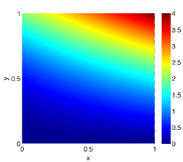
(a) x-velocity

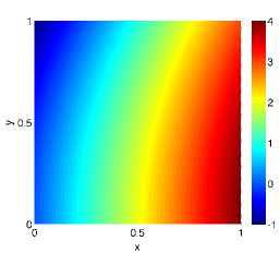
(b) y-velocity

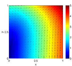
(c) velocity field

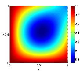
(d) pressure contour

Figure 3. Numerical $h$-convergence: contours of analytical solution.

Consider a unit square as the computational domain. For this and all subsequent numerical studies, the FEM utilizes structured meshes as depicted in Figure 2. The velocity and pressure functions for this problem are:

$$\mathbf{\bar{v}}(x,y)=\begin{Bmatrix}2y(x+y),\\ 4x-y^{2}.\end{Bmatrix}$$ (50a)

$$\bar{p}(x,y)=10-xy-\mathrm{sin}(\pi x)\mathrm{sin}(\pi y)$$ (50b)

Inserting the velocity and pressure functions back into the Darcy equation results in the following specific body force function:

$$\mathbf{\bar{b}}(x,y)=\frac{1}{\bar{\rho}}\begin{Bmatrix}\bar{\alpha}2y(x+y)-\pi\mathrm{cos}(\pi x)\mathrm{sin}(\pi y)-y\\ \bar{\alpha}(4x-y^{2})-\pi\mathrm{cos}(\pi y)\mathrm{sin}(\pi x)-x\end{Bmatrix}$$ (51)

Table 1. User-defined inputs for the numerical $h$-convergence problem.

Parameters	Value
$\bar{\beta}_{\mathrm{B}}$	0.1
$\bar{\beta}_{\mathrm{F}}$	0.5
$\bar{\alpha}$	1
$\bar{\rho}$	1
$\vartheta$	1
$h$-sizes	1/4, 1/8, 1/16, 1/32, 1/64

(a) LS: Q4 elements

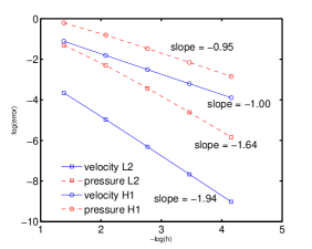
(b) LS: T3 elements

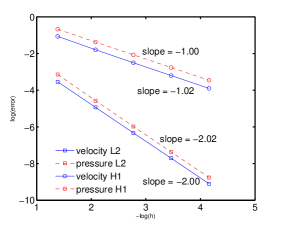
(c) VMS: Q4 elements

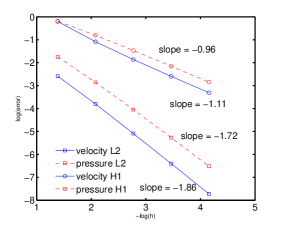
(d) VMS: T3 elements

Figure 4. Numerical $h$-convergence: error slopes for the MBF model

Table 2. Numerical $h$-convergence slopes for various Darcy models.

	LS formalism				VMS formalism
	D	MB	F	MBF	D	MB	F	MBF
Q4 $L_{2}$ error $v$	-2.00	-2.00	-1.99	-2.00	-1.99	-2.00	-1.99	-2.00
Q4 $H^{1}$ error $v$	-1.00	-1.00	-1.00	-1.00	-1.14	-1.04	-1.05	-1.02
Q4 $L_{2}$ error $p$	-1.95	-1.96	-1.99	-1.98	-2.01	-2.03	-2.02	-2.02
Q4 $H^{1}$ error $p$	-1.00	-1.00	-1.00	-1.00	-1.00	-1.00	-1.00	-1.00
T3 $L_{2}$ error $v$	- 1.97	-1.97	-1.84	-1.94	-1.84	-1.86	-1.81	-1.86
T3 $H^{1}$ error $v$	-1.01	-1.01	-1.00	-1.00	-1.13	-1.13	-1.07	-1.11
T3 $L_{2}$ error $p$	-1.62	-1.65	-1.62	-1.64	-1.69	-1.71	-1.70	-1.72
T3 $H^{1}$ error $p$	-0.95	-0.95	-0.95	-0.95	-0.96	-0.96	-0.96	-0.96

Normal components of the velocity function in equation (50) are prescribed as the boundary condition. A pressure of 10 is also prescribed at the bottom left corner to ensure uniqueness in the solution. Using the parameters listed in Table 1, Figure 3 depicts the analytical velocity and pressure solutions to which the finite element solutions shall be compared with. Since neither the pressure nor velocity functions depend on the drag coefficient, only the specific body force varies with respect to each Darcy model. The four Darcy models used are: the original Darcy (D), modified Barus (MB), Darcy-Forchheimer (F), and modified Darcy-Forchheimer Barus (MBF) models. The $L_{2}$ norm and $H^{1}$ seminorm error slopes for the modified Darcy-Forchheimer Barus models are depicted in Figure 4. Four-node quadrilateral (Q4) and three-node triangular (T3) elements are used to solve the problems, and Table 2 lists all the error slopes for the rest of the models.

It can be seen that the numerical solutions perform well; converged solutions should have error slopes of approximately -2.00 and -1.00 for $L_{2}$ norm and $H^{1}$ seminorm respectively. Though not shown, it has been found that the error slopes for all six models are similar to one another. Quadrilateral elements tend to exhibit faster convergence rates than triangular elements, and one can expect even faster rates for higher order elements like the nine-node quadrilateral Q9 and six-node triangular T6.

4.3. Quarter five-spot problem

Figure 5. Quarter five-spot problem: A pictorial description.

This section presents numerical results for a quarter spot problem as depicted in Figure 5. In many enhance oil recovery applications, there is an injection well centered around four production wells.

Table 3. User-defined inputs for the quarter five-spot problem: Darcy model.

Parameters	Value
$\bar{\alpha}$	1
$\bar{\rho}$	1
$\bar{\mathbf{b}}$	0
$Nele$	400
$\bar{p}(1,1)$	1
$\bar{v}_{x}(0,0)$, $\bar{v}_{y}(0,0)$	1
$\bar{v}_{x}(1,1)$, $\bar{v}_{y}(1,1)$	1

When carbon-dioxide is injected into the ground, the pressure build up pushes oil out through the four injection wells. This schematic forms what is often known as the five spot problem. Numerical results will exhibit elliptic singularities near the injection and production wells and provide a good benchmark to test the robustness of the finite element formulations. Due to the symmetric nature of the problem, only the top right quadrant is considered in the analysis. There is no specific body force or volumetric/sink source, and a pressure of $\bar{p}_{0}=1$ is prescribed at the production well or top right node. Since it has been shown in previous sections that the FEM developed performs well for both Q4 and T3 elements, only quadrilateral elements Q4 and Q9 will be used to simulate all proceeding numerical simulations.

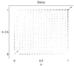
(a) LS velocity vector field

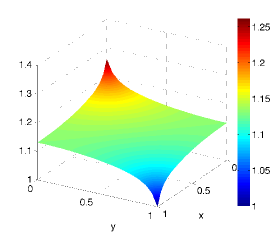
(b) LS pressure contour

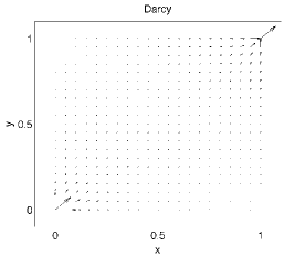
(c) VMS velocity vector field

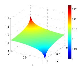
(d) VMS pressure contour

Figure 6. Quarter five-spot problem: Q4 solutions for Darcy model

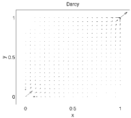
(a) LS velocity vector field

(b) LS pressure contour

(c) VMS velocity vector field

(d) VMS pressure contour

Figure 7. Quarter five-spot problem: Q9 solutions for Darcy model

Consider a case where there is $\sqrt{2}$ units of flow through the unit square quadrant. To attain this flow rate, one needs to know the amount of pressure needed at the injection well (i.e., the bottom left node). Using Q4 elements and the parameters listed in Table 3, Figure 6 depicts the qualitative velocity vector field and the pressure contour. While both formalisms exhibit similar pressure contours, the velocity vector field generated from the LS method exhibits poor dispersion of flow concentration at both wells. Intuitively, the profile of Figure 6(a) makes little to no physical sense so when using the LSFEM, neither Q4 nor any other first order elements can be used to accurately model velocity contours.

However, when higher order elements are used, the LS velocity vector field resembles that of the VMS. Figure 7 depicts the results using Q9 elements. It should be noted that the pressure contours remain the same regardless of the element order used. Realistic pressure profiles can be obtained using either formalism or element type, but obtaining velocity and flow solutions with the LSFEM necessitates the use of Q9 or higher ordered elements.

4.3.1. Least-squares weighting

For all original Darcy model problems up to this point, the non-dimensionalized drag coefficient equals one, so the two possible LS weightings $\mathbf{A}$ in equation (43) would be the same. When $\bar{\alpha}$ no longer equals one, weighting number 2 begins to have a significant impact on the numerical solutions. Herein, the injection pressure shall be obtained using various drag coefficients (all other user-defined parameters are as stated in Table 3). The VMS formalism serves as a benchmark for the two LS weightings.

Table 4. Quarter five-spot problem: Injection pressure comparison for different LS weightings.

$\bar{\alpha}:$	1	20	50	100	250	500	1000
LS weight 1 Q4:	1.26	6.03	12.56	21.57	47.29	91.38	180.57
LS weight 1 Q9:	1.27	6.38	14.44	27.76	67.17	132.63	263.77
LS weight 2 Q4:	1.26	6.19	13.90	26.67	64.43	126.00	244.97
LS weight 2 Q9:	1.27	6.38	14.46	27.92	68.31	135.60	269.37
VMS Q4:	1.27	6.37	14.42	27.84	68.09	135.18	269.37
VMS Q9:	1.27	6.38	14.46	27.93	68.32	135.63	270.27

From Table 4, it is seen that a divergence in the solutions occurs as the drag coefficient increases. LS formalism using Q9 elements has comparable stiffness to that of VMS formalism using Q4 elements, but as the drag increases, the VMS formalism using Q9 elements requires larger and larger pressures. Nonetheless, all the solutions show a linear relationship between drag and injection pressure. For highly viscous or lowly permeable reservoirs, one has to apply more pressure in order to attain or expect a certain flow. If drag is a function of pressure and/or velocity, one can expect even greater injection pressures.

4.3.2. Comparison of beta coefficients, pressure profiles, and linearization types

This next study shall illustrate the effect the Barus and Forchheimer coefficients have on the pressure profile and convergence of residuals. For pressure dependent viscosities, the Barus coefficient for most oils range between 15 to 35 GPa^-1 (see reference [62]) which translates to a non-dimensionalized coefficient of roughly 0.001 to 0.004.

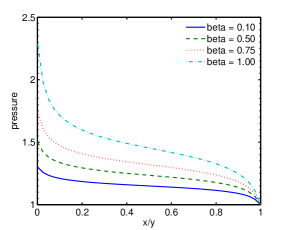
(a) Modified Barus - LS Q9

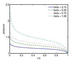
(b) Modified Barus - VMS Q9

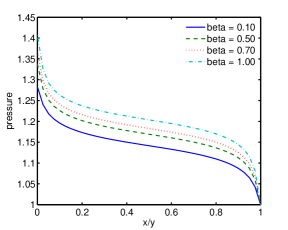
(c) Darcy-Forchheimer - LS Q9

(d) Darcy-Forchheimer - VMS Q9

Figure 8. Quarter five-spot problem: pressure profile vs various $\beta_{\mathrm{B}}$ and $\beta_{\mathrm{F}}$

However, for the purpose of this experiment, much higher Barus coefficients shall be used. The same Barus coefficients used will also be used for the Forchheimer coefficients. The relationship between the coefficients and the number of iterations needed to converge the residuals will also be shown for both linearization types.

Figure 8 depicts the pressure profile diagonally across the quarter region. Various beta values were used for the modified Barus and Darcy-Forchheimer models (assume both $\bar{\beta}_{\mathrm{B}}$ and $\bar{\beta}_{\mathrm{F}}$ to be denoted by the same $\bar{\beta}$). Overall the LS and VMS formalisms generate similar results.

Table 5. Quarter five-spot problem: Picard vs. consistent linearization iteration counts for modified Barus model with $\bar{\beta}_{\mathrm{B}}=0.6$. The top table corresponds with LS formalism, and the bottom table corresponds with VMS formalism. Q9 elements are used

LS formalism:	Picard’s linearization		consistent linearization
Iteration no. $(i)$	$\mathbf{\bar{v}}$ residual	$\bar{p}$ residual	$\mathbf{\bar{v}}$ residual	$\bar{p}$ residual
1	1.637285e+01	2.793981e-01	1.637323e+01	2.853694e-01
2	6.735667e-04	6.821094e-03	1.578203e-02	6.444641e-02
3	8.721274e-05	1.096770e-03	7.696835e-04	1.025242e-02
4	8.150045e-06	1.225905e-04	7.976516e-07	2.339612e-05
5	5.881603e-07	1.019954e-05	2.200057e-10	8.554086e-09
6	3.455235e-08	6.755041e-07	5.434345e-14	3.075479e-12
7	1.712434e-09	3.720906e-08
8	7.340079e-11	1.755375e-09
9	2.770668e-12	7.240625e-11
VMS formalism:	Picard’s linearization		consistent linearization
Iteration no. $(i)$	$\mathbf{\bar{v}}$ residual	$\bar{p}$ residual	$\mathbf{\bar{v}}$ residual	$\bar{p}$ residual
1	6.474444e-02	1.376963e-01	2.086226e-01	1.376963e-01
2	5.513505e-03	3.454112e-03	1.506223e-01	3.675604e-02
3	4.187925e-04	5.555865e-04	4.681837e-03	1.500411e-02
4	2.726750e-05	6.208117e-05	6.326269e-06	9.377515e-05
5	1.551030e-06	5.160684e-06	9.996752e-10	5.528937e-08
6	7.728631e-08	3.412260e-07	1.985333e-13	1.116834e-11
7	3.389569e-09	1.874543e-08
8	1.318682e-10	8.807571e-10

As the coefficient $\bar{\beta}$ increase, the pressure gradients at the two wells steepen. The modified Barus model exhibits the steepest gradients which is expected. The Darcy-Forchheimer solutions also exhibit increases in the injection pressure, but the qualitative nature of the pressure gradients near the wells are slightly different. Since the modified and Darcy-Forchheimer models rely on separate non-Darcy coefficients and different dependent variables, no true comparisons can be drawn. In the next Section however, distinction of results from pressure dependent and velocity dependent drag coefficients will become more evident.

It should be noted that the pressure profiles in Figure 8 were generated using Picard’s linearization (i.e. $\vartheta=0$). While Picard’s and consistent linearization theoretically yield the same results, the residual convergence schemes differ. Table 5 contains the iteration count and residual norms for the modified Barus model evaluated at $\bar{\beta}_{\mathrm{B}}=0.6$. Consistent linearization exhibits terminal quadratic convergence whereas Picard’s linearization exhibits terminal linear convergence. As the betas and/or applied pressure increases, the number of iterations needed increases.

4.3.3. Modified Darcy-Forchheimer numerical results

So far it has been established in this section that quadratic elements and LS weight 2 are preferred for the LS formalism. Numerical simulations have also shown that high Barus and Forchheimer coefficients yield results that differ quantitatively from the original Darcy model. This next example shall study the effects of combining the Darcy models and employs a finer mesh.

Table 6. Quarter five-spot problem: expected injection pressures for various Darcy models and mesh sizes

$Nele$	formalism	D	MB	F	MBF
400	LS	1.2692	1.5017	1.3382	1.5806
400	VMS	1.2693	1.5020	1.3382	1.5809
900	LS	1.1967	1.3538	1.2430	1.4045
900	VMS	1.1967	1.3539	1.2430	1.4047

Using the same boundary conditions as before, a non-dimensionalized Barus and Forchheimer coefficient of 0.5 and 0.5 shall be used. Since the qualitative nature of the pressure contours are similar no matter which model is used, only the required injection pressure is listed. It can be seen from the results in Table 6 that refining the mesh lowers the pressure. For problems where flow quantities are fixed, coarse meshes over predict the required pressure needed. The Barus, linear, and Forchheimer models all predict pressures greater than that of the original Darcy model, and when the modified Darcy-Forchheimer models are employed, we get even higher pressures. The original Darcy model under predicts the amount of pressure needed so it is important to use the modified Darcy-Forchheimer models to attain an accurate visualization of the pressure contours.

4.3.4. Minimum dissipation

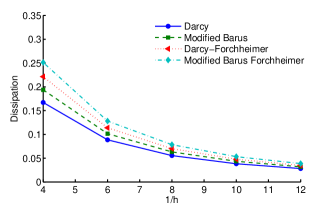
(a) LS formalism

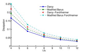
(b) VMS formalism

Figure 9. Quarter five-spot problem: dissipation vs $h$-size

Dissipation shall now be measured for this problem using various mesh sizes (Barus and Forchheimer coefficients of 0.1 and 0.5 shall be used respectively). The $h$-sizes used for this problem are 1/4, 1/6, 1/8, 1/10, and 1/12. All four Darcy models are evaluated using both formalisms, and the results can be found in Figure 9. It is seen that as the mesh gets finer the dissipation becomes smaller hence satisfying the minimum dissipation inequality. Though the LS formalism yields slightly higher dissipations, the results of both formalisms are very similar.

4.4. Three-dimensional constant flow

It has been claimed in references [12, 26] that the VMS mixed formulation for Darcy model is the only known mixed formulation that satisfies constant flow patch test in three dimensions on non-constant Jacobian finite elements. We show that the mixed formulation based on least-squares formalism also satisfy the constant patch test in three dimensions for Darcy model. We shall also use the test problem to show that the proposed mixed formulations perform well even for other modifications of the Darcy model. (It should be emphasized that this problem can be considered as a patch test only for Darcy model, and not for modified Darcy-Forchheimer, as the exact solution under the modified Darcy-Forchheimer model will not be neither linear nor constant.)

The computational domain is a unit cube, which is meshed using eight-node brick elements. Normal components of the velocity are prescribed as unity on the y-z planes at x = 0 and x = 1. The other four planes have normal components of velocity equal to zero, and a pressure value of zero is prescribed at (0,0,0) to ensure uniqueness to the solution. Using the values defined in Table 7, the LS results for the original Darcy, modified Barus, Darcy-Forchheimer, and modified Darcy-Forchheimer Barus models are shown in Figure 10. Clearly, the LS-based mixed formulation satisfies the constant patch test.

Table 7. User-defined inputs for the three-dimensional problem

Parameter	Value
$\bar{\beta}_{\mathrm{B}}$	0.5
$\bar{\beta}_{\mathrm{F}}$	1
$\bar{k}$	1
$\bar{\mu}_{0}$	1
$\vartheta$	1
$\bar{\mathbf{b}}(\mathbf{x})$	0
$Nele$	216

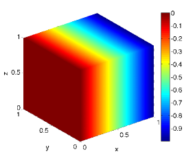
(a) Darcy model

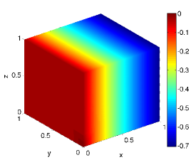
(b) Modified Barus

(c) Darcy-Forchheimer

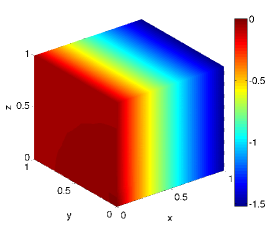
(d) Modified Darcy-Forchheimer Barus

Figure 10. Three dimensional problem: Pressure contours using LS formalism.

5. ENHANCED OIL RECOVERY APPLICATIONS

It has been shown in the previous section that the proposed mixed formulations perform well for the benchmark tests and that various modifications to the Darcy model have a significant impact on the results. This section focuses on relevant enhanced oil recovery applications, which are more complex by nature. Pressure contours, flow rates, and errors in the local/element-wise mass balance. Q9 elements shall be used for each problem.

5.1. Oil reservoir problem

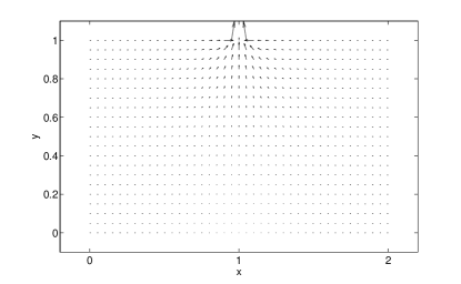
Figure 12. Oil reservoir problem: qualitative velocity vector field

For high pressure applications like enhanced oil recovery, one is interested in the quantitative and qualitative nature of the pressure contours and velocities within the oil reservoir. The pictorial description of a typical oil reservoir is depicted in Figure 11. Injection wells are located on either side the production well, and carbon-dioxide is pumped into the reservoir to ease the extraction of raw oil through the production well. The parameters used for this study are listed in Table 8. All Darcy models and finite element formulations are expected to yield differing flow patterns, but the general qualitative velocity vector can be depicted in Figure 12. As the oil fluid nears the production well, the Darcy velocities increases.

Table 8. User-defined inputs for the oil reservoir problem

Parameter	Value
$\bar{\beta}_{\mathrm{B}}$	0.005
$\bar{\beta}_{\mathrm{F}}$	0.01
$\bar{k}$	1
$\bar{\mu}_{0}$	1
$\bar{\rho}$	1
$\vartheta$	1
$\bar{\mathbf{b}}(\mathbf{x})$	$\begin{Bmatrix}0;-1\\ \end{Bmatrix}$
$Nele$	1600
$\bar{p}_{\mathrm{enh}}$	1000

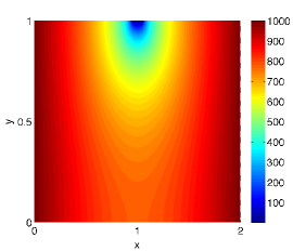
(a) Darcy model

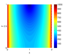
(b) Modified Barus

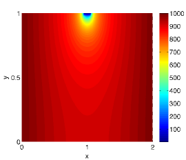
(c) Darcy-Forchheimer

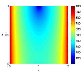
(d) Modified Darcy-Forchheimer Barus

Figure 13. Oil reservoir problem: pressure contours using LS formalism

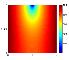
(a) Darcy model

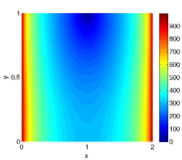
(b) Modified Barus

(c) Darcy-Forchheimer

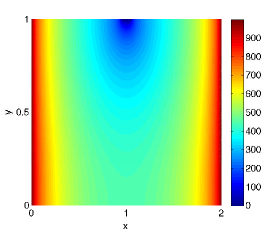
(d) Modified Darcy-Forchheimer Barus

Figure 14. Oil reservoir problem: pressure contours using VMS formalism

Pressure contours within the oil reservoirs are important to know because high pressures can result in cracking of the solid. Figures 13 and 14 contain the pressure contours using the LS and VMS formalisms respectively.

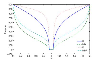
(a) LS formalism

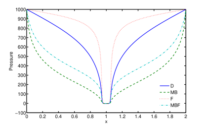
(b) VMS formalism

Figure 15. Oil reservoir problem: comparison of pressure profiles at $y=1$

It can be seen from each model that the pressure contours within the reservoirs vary both qualitatively and quantitatively. For the Barus model, there are steep pressure gradients near the injection well, and the pressures within the reservoir are generally smaller than that of the Darcy model. However, the Darcy-Forchheimer models exhibits steep pressure gradients near the production well, thus predicting higher pressures throughout the reservoir. While pressure dependent viscosity may yield favorable pressure contours, one has to account for increases in pressure due to inertial effects, so combining the Barus and Forchheimer models should yield the most accurate results. Figure 15 depicts the pressure profiles of all models and formalisms at the top most interface of the reservoir.

It should be noted that there are some minor differences in the pressure profiles between the LS and VMS formalisms. While both formalisms have strongly prescribed velocity boundary conditions, the VMS boundary condition for pressures are weakly prescribed and consequently exhibit some oscillations. The oscillations diminish with mesh refinement, but one must recognize the potential ramifications oscillatory boundary conditions may have on the solutions, especially for more complex prescribed pressures.

In reservoir simulations, another quantity of interest is the outflow of raw oil. The flow rate or total flux at the production well is calculated using

$$\int_{\Gamma^{p}}\mathbf{\bar{v}}\cdot\mathbf{\hat{n}}\;\mathrm{d}\Gamma,$$ (52)

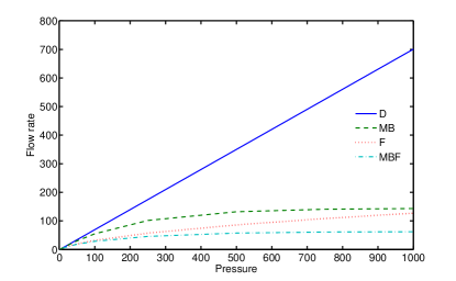
(a) LS formalism

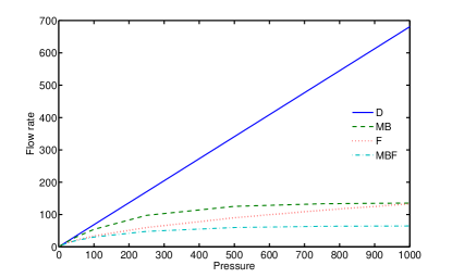
(b) VMS formalism

Figure 16. Oil reservoir problem: comparison of injection pressures vs. flow rates

where $\Gamma^{p}$ corresponds with the prescribed atmospheric pressure boundary. In Figure 16, a comparison of flow rates versus prescribed pressures is shown for both formalisms. The original Darcy models predict a linear relationship between prescribed pressures and flow rates but the non-linear Darcy models exhibit ceiling fluxes. As the pressure increases, the original Darcy models becomes increasingly unreliable as it over predicts the amount of oil production one can expect. It is interesting to note that for both the Darcy and Barus models, the LS formalism predicts higher flows for a fixed injection pressure whereas the VMS formalism predicts higher Forchheimer flow rates. Nevertheless, the ceiling fluxes for the Barus and Forchheimer models differ for various betas, but combining the two models will always yield smaller flow rates.

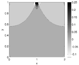
(a) Darcy model

(b) Modified Barus

(c) Darcy-Forchheimer

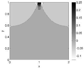
(d) Modified Darcy-Forchheimer Barus

Figure 17. Oil reservoir problem: ratios of local mass balance error over total predicted flux using LS formalism

As stated in Section 1, neither the LS nor VMS formalisms have local mass conservation. The ratios of local mass balance errors over the total predicted flux for the modified Darcy-Forchheimer Barus models are shown in Figure 17 and 18. When one encounters high velocity contours, one can also expect higher local mass balancing errors. The calculations show that all models exhibit the greatest errors near the production wells. It is interesting to note that while both formalisms predict roughly the same velocity flow rates, the VMS formalism shows greater local mass balancing error. Ratios of 0.25-0.35 are considered quite large, but for lower pressure and velocity applications, the ratios should be much smaller.

5.2. Multilayer reservoir problem

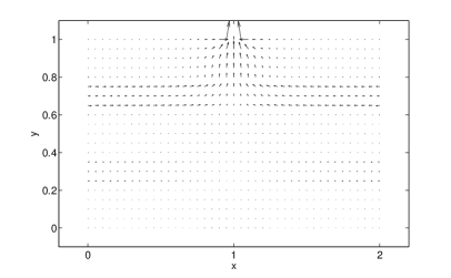
Figure 20. Layered reservoir problem: qualitative velocity vector field

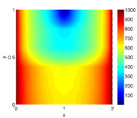
(b) Modified Barus

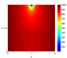
(c) Darcy-Forchheimer

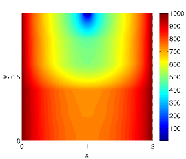
(d) Modified Darcy-Forchheimer Barus

Figure 21. Layered reservoir problem: pressure contours using LS formalism

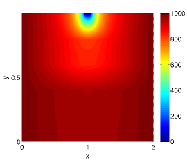
(a) Darcy model

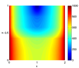
(b) Modified Barus

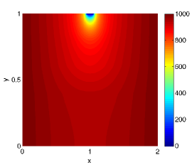
(c) Darcy-Forchheimer

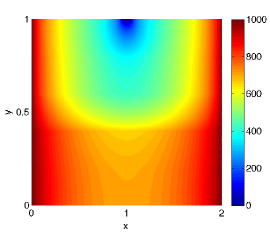
(d) Modified Darcy-Forchheimer Barus

Figure 22. Layered reservoir problem: pressure contours using VMS formalism

One may not always encounter constant permeability within the subsurface. Some layers within the oil reservoir may consist of coarse sands while others may consist of less permeable material. This numerical experiment shall study the effect varying permeability regions has on the pressure contours, flow rates, and local mass balance errors. Consider the domain depicted in Figure 19 with the same boundary conditions as that in Figure 11. Regions with higher permeability have larger velocities as depicted in Figure 20. The parameters used for this problem are listed in Table 9, and the pressure contours for LS and VMS formalisms are depicted in Figures 21 and 22 respectively.

Table 9. User-defined inputs for the layered reservoir problem

Parameter	Value
$\bar{\beta}_{\mathrm{B}}$	0.005
$\bar{\beta}_{\mathrm{F}}$	0.01
$\bar{k}$	varies
$\bar{\mu}_{0}$	1
$\bar{\rho}$	1
$\vartheta$	1
$\bar{\mathbf{b}}(\mathbf{x})$	$\begin{Bmatrix}0;-1\\ \end{Bmatrix}$
$Nele$	3200
$\bar{p}_{\mathrm{enh}}$	1000

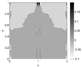
(a) Darcy model

(b) Modified Barus

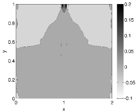
(c) Darcy-Forchheimer

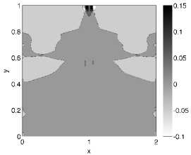
(d) Modified Darcy-Forchheimer Barus

Figure 23. Layered reservoir problem: ratios of local mass balance error over total predicted flux using LS formalism

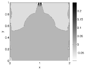
(a) Darcy model

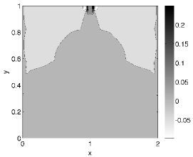
(b) Modified Barus

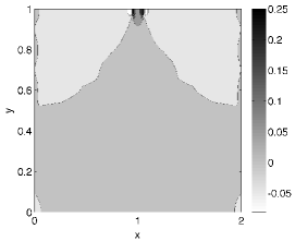
(c) Darcy-Forchheimer

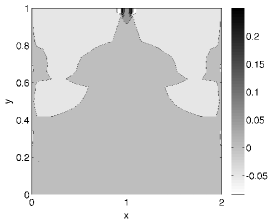
(d) Modified Darcy-Forchheimer Barus

Figure 24. Layered reservoir problem: ratios of local mass balance error over total predicted flux using VMS formalism

Results show that the layers with higher permeability contain higher pressures and that steep gradients occur at the interfaces between the layers. The LS formalism predicts higher pressures and larger flow rates for the Darcy and modified Barus models as seen from Table 10. Like with the previous oil reservoir problem, the VMS formalism predicts higher flow rates for the Darcy-Forchheimer model. The ratio of local mass balance errors and total predicted fluxes are depicted in Figures 23 and 24. While the VMS formalisms still have slightly higher errors, the overall error ratios for this problem are smaller despite having larger flow rates.

Table 10. Layered reservoir problem: flow rates for LS and VMS formalism at $\bar{p}_{\mathrm{enh}}$ = 1000

Darcy models:	D	MB	F	MBF
LS	1038	210	133	75
VMS	1025	204	137	77

5.3. Flow in a porous media with staggered impervious zones

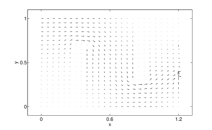
Figure 26. Staggered impervious zones problem: qualitative velocity vector field

Consider flow through a region with staggered impervious zones in Figure 25. In any heterogeneous flow through porous media applications, one may encounter domains where oil must flow through a complex domain with many impervious regions. The qualitative velocity vector field in Figure 26 indicates that higher flows occur around the sharp bends.

Table 11. User-defined inputs for the staggered impervious zones problem

Parameter	Value
$\bar{\beta}_{\mathrm{B}}$	0.005
$\bar{\beta}_{\mathrm{F}}$	0.01
$\bar{k}$	1
$\bar{\mu}_{0}$	1
$\bar{\rho}$	1
$\vartheta$	1
$\bar{\mathbf{b}}$	0
Element type	Q9
$Nele$	1696
$\bar{p}_{\mathrm{enh}}$	1000

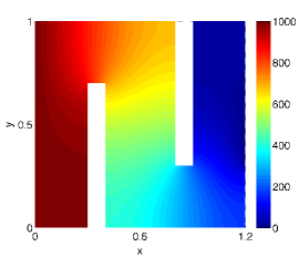
(a) Darcy model

(b) Modified Barus

(c) Darcy-Forchheimer

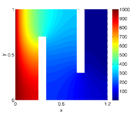
(d) Modified Darcy-Forchheimer Barus

Figure 27. Staggered impervious zones problem: pressure contours using LS formalism

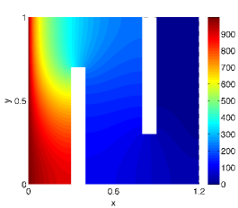
(b) Modified Barus

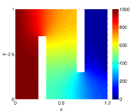
(c) Darcy-Forchheimer

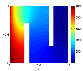
(d) Modified Darcy-Forchheimer Barus

Figure 28. Staggered impervious zones problem: pressure contours using VMS formalism

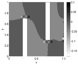
(a) Darcy model

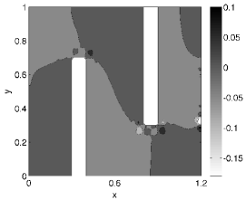
(b) Modified Barus

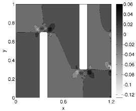
(c) Darcy-Forchheimer

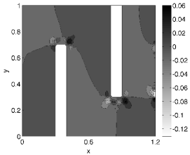
(d) Modified Darcy-Forchheimer Barus

Figure 29. Staggered impervious zones problem: ratios of local mass balance error over total predicted flux using LS formalism

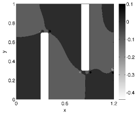
(a) Darcy model

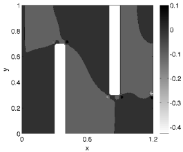
(b) Modified Barus

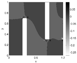
(c) Darcy-Forchheimer

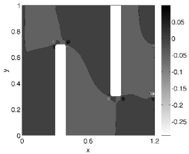
(d) Modified Darcy-Forchheimer Barus

Figure 30. Staggered impervious zones problem: ratios of local mass balance error over total predicted flux using VMS formalism

The pressure contours are depicted in Figures 27 and 28. The same non-dimensionalized injection pressure has been prescribed for this problem (see Table 11 for key parameters used in this problem), and it can still be seen that the different Darcy models make an impact on the qualitative nature of the pressure contours. Again, the LS formalism yields higher pressures throughout the domain and predicts larger flow rates as seen in Table 12. Errors in the local mass balance tend to be greatest in regions with high velocities (i.e., the sharp bends around the impervious layers). Local mass balancing errors are shown in Figures 29 and 30.

Table 12. Staggered impervious zones problem: flow rates for LS and VMS formalism at $\bar{p}_{\mathrm{enh}}$ = 1000

Darcy models:	D	MB	F	MBF
LS	150.6	31.9	50.4	24.3
VMS	131.1	26.5	47.9	20.3

6. CONCLUDING REMARKS

The work in this thesis proposes a modification to the standard Darcy model that takes into account both the dependence of the viscosity on the pressure and the inertial effects, which have been observed in many physical experiments. The current models in the literature consider either of the effects but not both. The proposed model will be particularly important for predictive simulations of applications involving high pressures and high velocities (e.g., enhanced oil recovery). This modification has been referred to as the modified Darcy-Forchheimer model. It has been shown numerically that the results obtained by taking into account the dependence of drag coefficient on the pressure and on the velocity are both qualitatively and quantitatively different from that the results obtained using the standard Darcy model, Darcy-Forchheimer equation (which neglects the dependence of drag coefficient and viscosity on the pressure) or modified Darcy model [3, 20] (which neglects the dependence of the drag coefficient on the velocity).

This thesis has also developed stable mixed finite element formulations for the resulting governing equations using two different approaches: VMS formalism and LS formalism. Using numerical experiments, we have compared their merits and demerits.

The LS formulation has more terms to evaluate than the VMS formulation, and hence the LS formulation is slightly more computationally expensive than the VMS formulation. However, it should be emphasized that this is not significant in a parallel setting as element-level calculations are embarrassingly parallel. It is also observed that the LS formulation with $p$-refinement produces accurate results. Another point that is worth mentioning is that the VMS formalism weakly prescribes pressure boundary conditions, and it has been shown that minor oscillations occur when meshes are not adequately refined. The error in element-wise / local mass balance for various Darcy-type models is also quantified, and the error becomes significant when there are large pressures and velocities.

There are several ways one can extend the research work presented in this thesis. On the modeling front, a good but difficult research problem is to develop mathematical models that couple deformation and damage of the porous solid with the flow aspects and reactive transport across several spatial and temporal scales. The following are some possible future works on the numerical front:

1. Develop mixed finite element formulations with better local mass balance property under equal-order interpolation for the pressure and the velocity.

2. Develop multi-scale models by coupling continuum / macro-scale flow models with meso-scale models (e.g., lattice Boltzmann models). The advantage is that meso-scale models can easily handle complex pore structure, which may not computationally feasible if one uses only a macro-scale model.

3. Another important but difficult problem is to develop numerical upscaling techniques for heterogeneous porous media. In layman terms, numerical upscaling captures fine-scale features on coarse computational grids.

4. Develop stable and accurate coupling algorithms for coupling flow, deformation and transport aspects.

On the computer implementation front, a possible work is to implement the mixed formulations taking the advantage of GPU processors, and implementing on heterogeneous parallel computing environment.

Figure 11. Oil reservoir problem. Top figure is the pictorial description of enhanced oil recovery, and the bottom figure is the idealized computational domain with appropriate boundary conditions.

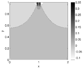
(a) Darcy model

(b) Modified Barus

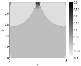
(c) Darcy-Forchheimer

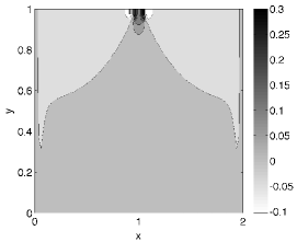
(d) Modified Darcy-Forchheimer Barus

Figure 18. Oil reservoir problem: ratios of local mass balance error over total predicted flux using VMS formalism

Figure 19. Layered reservoir problem: A pictorial description.

(a) Darcy model

Figure 25. Staggered impervious zones problem: A pictorial description.

(a) Darcy model

References

- [1] H. Darcy. Les Fontaines Publiques de la Ville de Dijon. Victor Dalmont, Paris, 1856.
- [2] S. P. Neuman. Theoretical derivation of Darcy’s law. Acta Mechanica, 25:153–170, 1977.
- [3] K. B. Nakshatrala and K. R. Rajagopal. A numerical study of fluids with pressure dependent viscosity flowing through a rigid porous medium. International Journal for Numerical Methods in Fluids, 67:342–368, 2011.
- [4] P. W. Bridgman. The Physics of High Pressure. MacMillan Company, New York, USA, 1931.
- [5] C. Barus. Isotherms, isopiestics and isometrics relative to viscosity. American Journal of Science, 45:87–96, 1893.
- [6] P. Forchheimer. Wasserbewegung durch Boden. Zeitschrift des Vereines Deutscher Ingeneieure, 45:1782–1788, 1901.
- [7] J. Bear. Dynamics of Fluids in Porous Media. Dover Publications, New York, 1988.
- [8] B. Jiang. The Least-Squares Finite Element Method: Theory and Applications in Computational Fluid Dynamics and Electromagnetics. Springer-Verlag, New York, USA, 1998.
- [9] T. J. R. Hughes. Multiscale phenomena: Green’s functions, the Dirichlet-to-Neumann formulation, subgrid scale models, bubbles and the origins of stabilized methods. Computer Methods in Applied Mechanics and Engineering, 127:387–401, 1995.
- [10] F. Brezzi and M. Fortin. Mixed and Hybrid Finite Element Methods, volume 15 of Springer Series in Computational Mathematics. Springer-Verlag, New York, USA, 1991.
- [11] P. B. Bochev and M. D. Gunzburger. Finite element methods of least-squares type. Society for Industrial and Applied Mathematics, 40:789–837, 1998.
- [12] K. B. Nakshatrala, D. Z. Turner, K. D. Hjelmstad, and A. Masud. A stabilized mixed finite element formulation for Darcy flow based on a multiscale decomposition of the solution. Computer Methods in Applied Mechanics and Engineering, 195:4036–4049, 2006.
- [13] J. Donea and A. Huerta. Finite Element Methods for Flow Problems. John Wiley & Sons, Inc., Chichester, UK, 2003.
- [14] K. A. Mardal, X. C. Tai, and R. Winther. A robust finite element method for Darcy-Stokes flow. SIAM Journal of Numerical Analysis, 40:1605–1631, 2002.
- [15] A. Masud. A stabilized mixed finite element method for Darcy-Stokes flow. International Journal for Numerical Methods in Fluids, 54:665–681, 2007.
- [16] O. Iliev, R. Lazarov, and J. Willems. Variational multiscale finite element method for flows in highly porous media. Multiscale Modeling and Simulation, 9:1350–1372, 2011.
- [17] M. R. Correa and A. F. D. Loula. Stabilized velocity post-processings for Darcy flow in heterogeneous porous media. Communications in Numerical Methods in Engineering, 23:461–489, 2007.
- [18] J. M. Urquiza, D. N. Dri, A. Garon, and M. C. Delfour. A numerical study of primal mixed finite element approximations of Darcy equations. Communications in Numerical Methods in Engineering, 22:901–915, 2006.
- [19] A. Masud and T. J. R. Hughes. A stabilized mixed finite element method for Darcy flow. Computer Methods in Applied Mechanics and Engineering, 191:4341–4370, 2002.
- [20] K. B. Nakshatrala and D. Z. Turner. A mixed formulation for a modification to Darcy equation based on Picard linearization and numerical solutions to large-scale realistic problems. Available on arXiv: http://arxiv.org/abs/1105.0706, 2013.
- [21] P. B. Bochev and M. D. Gunzburger. A locally conservative least-squares method for Darcy flows. Communications in Numerical Methods in Engineering, 24:97–110, 2008.
- [22] G. R. Barrenechea, L. P. Franca, and F. Valentin. A Petrov-Galerkin enriched method: A mass conservative finite element method for the Darcy equation. Computer Methods in Applied Mechanics and Engineering, 197:2449–2464, 2007.
- [23] S. Sun and J. Liu. A locally conservative finite element method based on piecewise constant enrichment of the continuous Galerkin method. SIAM Journal of Scientific Computing, 31:2528–2548, 2009.
- [24] J. Liu and X. Ye. A comparative study of locally conservative numerical methods for Darcy’s flows. Procedia Computer Science, 4:974–983, 2011.
- [25] D. Z. Turner, K. B. Nakshatrala, M. J. Martinez, and P. K. Notz. Modeling subsurface water resource systems involving heterogeneous porous media using the variational multiscale formulation. Journal of Hydrology, 428-429:1–14, 2011.
- [26] T. J. R. Hughes, A. Masud, and J. Wan. A stabilized mixed discontinuous Galerkin method for Darcy flow. Computer Methods in Applied Mechanics and Engineering, 195:3347–3381, 2006.
- [27] C. Truesdell. Rational Thermodynamics. Springer, New York, USA, 1984.
- [28] R. J. Atkin and R. E. Craine. Continuum theories of mixtures: Basic theory and historical development. The Quaterly Journal of Mechanics and Applied Mathematics, 29:209–244, 1976.
- [29] R. M. Bowen. Theory of mixtures. In A. C. Eringen, editor, Continuum Physics, volume III. Academic Press, New York, 1976.
- [30] R. McOwen. Partial Differential Equations: Methods and Applications. Prentice Hall, New Jersey, USA, 1996.
- [31] E. C. Andrade. Viscosity of liquids. Nature, 125:109–141, 1930.
- [32] H. J. van Leewen. The determination of the pressure viscosity coefficient of a lubricant through an accurate film thickness formula and accurate film thickness measurements. Journal of Engineering Tribology, 223:1143–1163, 2009.
- [33] M. Franta, J. Malek, and K. R. Rajagopal. On steady flows of fluids with pressure- and shear-dependent viscosities. Proceedings: Mathematical, Physical and Engineering Sciences, 461:651–670, 2005.
- [34] A. Him, M. Lanzendoerfer, and J. Stebel. Finite element approximation of flow of fluids with shear-rate- and pressure-dependent viscosity. IMA Journal of Numerical Analysis, 32:1604–1634, 2012.
- [35] H. C. Brinkman. A calculation of the viscous force exerted by a flowing fluid on a dense swarm of particles. Applied Scientific Research, A1:27–34, 1947.
- [36] S. Srinivasan and K. B. Nakshatrala. A stabilized mixed formulation for unsteady Brinkman equation based on the method of horizontal lines. International Journal for Numerical Methods in Fluids, 68:642–670, 2011.
- [37] A. Z. Szeri. Fluid Film Lubrication: Theory and Design. Cambridge University Press, Cambridge, UK, 2005.
- [38] E. H. Abramson. Viscosity of carbon dioxide measured to a pressure of 8 GPa and temperature of 673 K. Physical Review E, 80(021201), 2009.
- [39] V. Vesovic, W. A. Wakeham, G. A. Olchowy, J. V. Sengers, J. T. R. Watson, and J. Millat. The transport properties of carbon dioxide. Journal of Physical and Chemical Reference Data, 19:763–808, 1990.
- [40] E. Höglund. Influence of lubricant properties on elastohydrodynamic lubrication. Wear, 232:176–184, 1999.
- [41] S. Whitaker. The Forchheimer equation: A theoretical development. Transport in Porous Media, 25:27–61, 1996.
- [42] W. Sobieski and A. Trykozko. Sensitivity aspects of Forchheimer’s approximation. Transport in Porous Media, 89:155–164, 2011.
- [43] E. J. Park. Mixed finite element methods for generalized Forchheimer flow in porous media. Numerical Methods for Partial Differential Equations, 21:213–228, 2005.
- [44] H. Pan and H. Rui. Mixed element method for two-dimensional Darcy-Forchheimer model. Journal of Scientific Computing, 52:563–587, 2012.
- [45] B. Martin, K. J. Michael, and S. Harvey. Simulation and theory of two-phase flow in porous media. Physics Review A, 46:7680–7699, 1992.
- [46] D. E. Carlson, E. Fried, and D. A. Tortorelli. Geometrically-based consequences of internal constraints. Journal of Elasticity, 70:101–109, 2003.
- [47] O. M. O’Reilly and A. R. Srinivasa. On a decomposition of generalized constraint forces. Proceedings of the Royal Society of London, Series A, 457:1307–1313, 2001.
- [48] G. K. Batchelor. An Introduction to Fluid Dynamics. Cambridge University Press, New York, USA, 2000.
- [49] M. H. Sadd. Elasticity: Theory, Applications, and Numerics. Academic Press, Burlington, Massachusetts, 2009.
- [50] C. Truesdell and W. Noll. The Non-Linear Field Theories of Mechanics. Springer, Berlin, third edition, 2004.
- [51] E. Guazzelli and J. F. Morris. A Physical Introduction to Suspension Dynamics. Cambridge University Press, Cambridge, UK, 2012.
- [52] L. C. Evans. Partial Differential Equations. American Mathematical Society, Providence, Rhode Island, USA, 1998.
- [53] B. D. Reddy. Introductory Functional Analysis: With Applications to Boundary Value Problems and Finite Elements. Springer-Verlag, New York, USA, 1998.
- [54] J. T. Oden and L. F. Demkowicz. Applied Functional Analysis. CRC Press, Boca Raton, Florida, USA, second edition, 2010.
- [55] P. Chadwick. Continuum Mechanics: Concise Theory and Problems. Dover Publications, Inc., Minealo, New York, 1999.
- [56] M. Spivak. Calculus on Manifolds: A Modern Approach to Classical Theorems of Advanced Calculus. Westview Press, Massachusetts, USA, 1997.
- [57] G. A. Holzapfel. Nonlinear Solid Mechanics: A Continuum Approach for Engineering. John Wiley, New York, USA, 2000.
- [58] R. Glowinski. Numerical Methods for Nonlinear Variational Problems. Springer-Verlag, Leipzig, Germany, 2008.
- [59] G. S. Payette and J. N. Reddy. On the roles of minimization and linearization in least-squares finite element models of nonlinear boundary-value problems. Journal of Computational Physics, 230:3589–3613, 2011.
- [60] J. M. Deang and M. D. Gunzburger. Issues related to least-squares finite element methods for the Stokes equations. SIAM Journal on Scientific Computing, 20:878–906, 1999.
- [61] M. E. Gurtin. An Introduction to Continuum Mechanics. Academic Press, San Diego, USA, 1981.
- [62] G. Stachowiak and A. W. Batchelor. Engineering Tribology. Elsevier Science, Burlington, MA, third edition, 2011.