Interpretation of the unprecedentedly long-lived high-energy emission of GRB 130427A

Abstract

High energy photons ($>100$ MeV) are detected by the Fermi/LAT from GRB 130427A up to almost one day after the burst, with an extra hard spectral component being discovered in the high-energy afterglow. We show that this hard spectral component arises from afterglow synchrotron-self Compton emission. This scenario can explain the origin of $>10\,$GeV photons detected up to $\sim 30000$ s after the burst, which would be difficult to be explained by synchrotron radiation due to the limited maximum synchrotron photon energy. The lower energy multi-wavelength afterglow data can be fitted simultaneously by the afterglow synchrotron emission. The implication of detecting the SSC emission for the circumburst environment is discussed.

1. Introduction

The extended high-energy emission detected by Fermi/LAT is widely believed to arise from the electrons accelerated in the external–forward shock via the synchrotron radiation (e.g. Kumar & Barniol Duran, 2009, 2010). However, the maximum photon energy in this scenario is limited to be $\varepsilon_{\gamma,\rm max}=50\,\Gamma\,$MeV, where $50$ MeV is the maximum synchrotron photon in the rest frame of the shock and $\Gamma$ is the bulk Lorentz factor of the shock, which is usually $\lesssim 300$ at $\sim 100$s after the trigger (e.g. Piran & Nakar, 2010; Barniol Duran & Kumar, 2011). So the detection of $>10\,$GeV photons after 100 s poses a challenge for the synchrotron emission scenario (Piran & Nakar, 2010; Sagi & Nakar, 2012). Considering the above difficulty, Wang et al. (2013) recently proposed that the afterglow synchrotron self-Compton (SSC) emission or external inverse-Compton of central X-ray emission (Wang et al., 2006) is likely responsible for the late-time $>10\,$GeV photons seen in some LAT GRBs.

GRB 130427A triggered the Fermi/GBM with a fluence of $2\times 10^{−3}$erg cm^-2 in 10-1000 keV within a duration of $T_{90}=138$s (von Kienlin, 2013). It was later localized at $z\simeq 0.34$ (Flores et al., 2013; Levan et al., 2013; Xu et al., 2013a), implying an isotropic energy of $7.8\times 10^{53}\,$erg (Kann & Schulze, 2013). Unprecedentedly, $>100\,$MeV emissions are detected well beyond the prompt emission phase up to about one day after the burst, including fifteen $>10\,$GeV photons detected up to $\sim 30000$s and one 95.3 GeV photon arrived at 243s after the trigger (Zhu et al., 2013; Tam et al., 2013). It was suggested that these late-time high-energy photons may arise from inverse-Compton processes (Fan et al., 2013; Wang et al., 2013). Further evidence comes from the presence of a hard spectral component (the photon index $\Gamma_{\rm ph}=-1.4\pm 0.1$) above $2.5\pm 1.1\,$GeV (Tam et al., 2013) in the late afterglow, which has signatures well consistent with the prediction of the afterglow synchrotron self-Compton emission (Zhang & Mészáros, 2001; Sari & Esin, 2001; Zou et al., 2009). In this Letter, we will verify this possibility by modeling the multi-band (from radio to GeV bands) data of this burst. Hereafter, we denote by $Q_{x}$ the value of the quantity $Q$ in units of $10^{x}$.

2. A brief overview of the model

In the standard synchrotron afterglow spectrum, there are three break frequencies, i.e. $\nu_{a}$, $\nu_{m}$ and $\nu_{c}$, which are caused by synchrotron self-absorption (SSA), electron injection and electron cooling respectively. According to (e.g. Sari et al., 1998; Wijers & Galama, 1999), these three characteristic frequencies are given by

$$\nu_{{\rm m}}=1.1\times 10^{18}\,f^{2}(p)\epsilon_{e,-1}^{2}E_{54}^{1/2}\epsilon_{{\rm B},-5}^{1/2}(1+z)^{1/2}T^{-3/2}{\rm Hz},$$ (1)

$$\nu_{{\rm c}}=1.1\times 10^{17}\,E_{54}^{-1/2}n_{0}^{-1}\epsilon_{{\rm B},-5}^{-3/2}\left(\frac{1+Y}{100}\right)^{-2}(1+z)^{-1/2}T^{-1/2}{\rm Hz},$$ (2)

and

$$\nu_{a}=2.7\times 10^{10}\,f^{-1}(p)E_{54}^{1/5}\epsilon_{e,-1}^{-1}\epsilon_{B,-5}^{1/5}n_{0}^{3/5}(1+z)^{-1},$$ (3)

in the case that $\nu_{a}<\nu_{m}<\nu_{c}$, which is usually true under typical parameter values. In the above three equations, $T$ is the time in the observer’s frame since the trigger time, $z$ is the redshift of the burst, $f(p)=6(p-2)/(p-1)$ with $p$ being the electron index, $E$ is the isotropic kinetic energy of the GRB outflow and $n$ is the number density of the circumburst medium. For an interstellar medium (ISM) circumburst environment, $n$ is a constant while for a stellar wind circumburst environment, it is inversely proportional to the square of the shock radius. $\epsilon_{{\rm e}}$ and $\epsilon_{{\rm B}}$ are the equipartition factors for the energy in electrons and magnetic field in the shock respectively. In the expression of $\nu_{c}$, $Y$ is the Compton parameter evaluating the effect of SSC cooling on the synchrotron spectrum. In the Thomson scattering limit, $Y=Y_{0}\simeq(\frac{\epsilon_{e}}{\epsilon_{B}})^{\frac{1}{4-p}}\left(\frac{\nu_{m}}{\nu_{c,\rm syn}}\right)^{\frac{p-2}{2(4-p)}}$ (Sari & Esin, 2001) if $Y\gg 1$, where $\nu_{c,\rm syn}$ is obtained by considering only the synchrotron cooling.

The time–integrated spectrum of high–energy emission from GRB 130427A can be modeled by a broken power-law with a soft component ($\Gamma_{\rm ph}=2.3\pm 0.1$) below the break energy $E_{b}=2.5\pm 1.1\,$GeV and a hard component ($\Gamma_{\rm ph}=1.4\pm 0.1$) above $E_{b}$ (Tam et al., 2013). It is natural to assume that synchrotron emission is dominant below $E_{b}$ while the SSC emission is dominant above $E_{b}$. As Tam et al. (2013), we assume $p=2.2$ in the following analysis. Thus, the synchrotron flux at $h\nu_{c}<100{\rm MeV}\leq h\nu_{\rm LAT}<E_{b}$ is given by

$$\begin{split}F_{\nu}(100\,{\rm MeV})=&7.0\,E_{54}^{1.05}\epsilon_{e,-1}^{1.2}\epsilon_{B,-5}^{0.05}(1+z)^{1.05}\\ &\times D_{L,28}^{-2}T^{-1.15}\left(\frac{h\nu}{100\,\rm MeV}\right)^{-1.1}\mu\rm Jy\end{split}$$ (4)

where $D_{L}$ is the luminosity distance. Here we neglect the inverse-Compton cooling for the electrons that radiate high-energy gamma-ray emission due to the deep Klein–Nishina (KN) scattering effect(Wang et al., 2010; Liu & Wang, 2011). The emission above $E_{b}$ can be interpreted as the SSC emission in the regime of $h\nu_{m}^{\rm ssc}<h\nu_{\rm LAT}<h\nu_{c}^{\rm ssc}$, where $\nu_{m}^{\rm ssc}$ and $\nu_{c}^{\rm ssc}$ are the corresponding break frequencies in the SSC spectrum. The SSC flux is given by (Sari & Esin, 2001)

$$\begin{split}F_{\nu}(10{\rm GeV})=&5.6\times 10^{-3}E_{54}^{1.7}n_{0}^{1.1}\epsilon_{e,-1}^{2.4}\epsilon_{B,-5}^{0.8}(1+z)^{1.5}\\ &\times D_{L,28}^{-2}T^{-1.1}\left(\frac{h\nu}{10\,\rm GeV}\right)^{-0.6}\mu\rm Jy\end{split}$$ (5)

Lower energy emission is produced by the forward shock synchrotron radiation. X-ray observation frequency is usually also in the fast cooling regime, i.e. $\nu_{m}<\nu_{c}<\nu_{X}$. But the KN suppression effect is not as important as in the case of $>100\,$MeV emission, so we need to consider the effect of SSC cooling on the synchrotron spectrum carefully. Thus, we have

$$\begin{split}F_{\nu}(10\,\rm keV)=&17\,E_{54}^{1.05}\epsilon_{e,-1}^{1.2}\epsilon_{B,-5}^{0.05}\left[\frac{1+Y(10\rm\,keV)}{10}\right]^{-1}\\ &\times(1+z)^{1.05}D_{L,28}^{-2}T^{-1.15}\left(\frac{h\nu}{10\,\rm keV}\right)^{-1.1}\rm mJy\end{split}$$ (6)

Here $Y(10{\rm\,keV})=f_{\rm KN}Y_{0}$ with $Y_{0}=U_{\rm syn}/U_{B}=110\,E_{54}^{0.056}n_{0}^{0.056}\epsilon_{e,-1}^{0.67}\epsilon_{B,-5}^{-0.44}(1+z)^{0.056}T^{-0.056}$ being the Compton parameter in the Thomson scattering limit as mentioned above, where $U_{\rm syn}$ and $U_{B}$ are the energy density of synchrotron radiation field and magnetic field respectively. The factor $f_{\rm KN}$ considers the KN effect on the electrons that emit $10\,$keV photons by synchrotron radiation. In the Thomson scattering regime $f_{\rm KN}=1$, while in the deep KN scattering regime $f_{\rm KN}\rightarrow 0$.

The KN effect will intervene in the inverse Compton cooling if the energy of the incident photon exceeds the rest energy of the scattering electron in its rest frame, i.e., $\gamma_{e}h\nu_{\rm KN}(1+z)/\Gamma\geq m_{e}c^{2}$, where $\gamma_{e}$ is the Lorentz factor of the electron in the comoving frame of the emitting region and $\nu_{\rm KN}$ is the critical frequency of the incidence photon measured in the observer’s frame. If the energy of a photon is larger than $h\nu_{\rm KN}$, the scatter will enter the KN regime with a suppressed cross section. The Lorentz factor of the electron emitting X-ray photons can be given by $\gamma_{\rm 10\,keV}=\left(\frac{2\pi m_{e}c\nu_{\rm X}(1+z)}{\Gamma eB}\right)^{1/2}$ and thus

$$\nu_{\rm KN,10\,keV}=2.8\times 10^{18}\,E_{54}^{1/4}\epsilon_{B,-5}^{1/4}(1+z)^{-3/4}\left(\frac{h\nu_{\rm X}}{10\,\rm keV}\right)^{1/2}T^{-3/4}$$ (7)

As $\nu_{\rm KN}\propto T^{-3/4}$, the KN suppression effect becomes more and more important at later time. As a rough estimate, $f_{\rm KN}$ can be given by

$$f_{\rm KN}=\frac{U_{\rm syn}(\nu<\nu_{\rm KN})}{U_{\rm syn}}\simeq\left\{\begin{array}[]{lll}0.06\left(\frac{\nu_{m}}{\nu_{c}}\right)^{0.4}\left(\frac{\nu_{\rm KN}}{\nu_{m}}\right)^{4/3}&\nu_{\rm KN}<\nu_{m},\\ 0.2\left(\frac{\nu_{\rm KN}}{\nu_{c}}\right)^{0.4}&\nu_{m}<\nu_{\rm KN}<\nu_{c},\\ 1-0.8\left(\frac{\nu_{\rm KN}}{\nu_{c}}\right)^{-0.1}&\nu_{c}<\nu_{\rm KN}\end{array}\right.$$ (8)

In a broad parameter space, we find $\nu_{m}<\nu_{\rm KN}<\nu_{c}$, leading to $f_{\rm KN}\simeq 0.1E_{54}^{0.3}n_{0}^{0.4}\epsilon_{B,-5}^{0.7}(1+z)^{0.1}[\frac{1+Y(10\,{\rm keV})}{10}]^{0.8}(\frac{h\nu}{10\rm keV})^{0.2}T^{-0.1}$.

Optical emission is typically in the frequency regime $\nu_{m}<\nu_{\rm Op}<\nu_{c}$, so the flux is given by

$$\begin{split}F_{\nu}({\rm R\,band})=&1.3\,E_{54}^{1.3}n_{0}^{0.5}\epsilon_{e,-1}^{1.2}\epsilon_{B,-5}^{0.8}(1+z)^{1.3}\\ &\times D_{L,28}^{-2}T^{-0.9}\left(\frac{\nu}{4.56\times 10^{14}\rm Hz}\right)^{-0.6}\rm Jy.\end{split}$$ (9)

The radio observation frequency could lie in the regime $\nu_{a}<\nu_{\rm Ra}<\nu_{m}$ or $\nu_{\rm Ra}<\nu_{a}<\nu_{m}$. In the former case,

$$\begin{split}F_{\nu}(5\,{\rm GHz})=&20\,E_{54}^{5/6}n_{0}^{1/2}\epsilon_{e,-1}^{-2/3}\epsilon_{B,-5}^{1/3}(1+z)^{5/6}\\ &\times D_{L,28}^{-2}T^{1/2}\left(\frac{\nu}{5\,\rm GHz}\right)^{1/3}\mu\rm Jy,\end{split}$$ (10)

while in the latter case,

$$\begin{split}F_{\nu}(5\,{\rm GHz})=&1.3\,E_{54}^{1/2}n_{0}^{-1/2}\epsilon_{e,-1}(1+z)^{5/2}\\ &\times D_{L,28}^{-2}T^{1/2}\left(\frac{\nu}{5\,\rm GHz}\right)^{2}\mu\rm Jy.\end{split}$$ (11)

We note that in previous works, modeling of the multi-band light curves of LAT-detected GRBs usually result in a low circumburst density $<10^{-2}\,\rm cm^{-3}$ (e.g. Cenko et al., 2011; Liu & Wang, 2011; He et al., 2011). In a low-density environment, SSC flux would be severely suppressed. We here point out that the low-density result is mainly due to neglect of the KN effect in modeling the X-ray afterglows. We now briefly show that considering the KN effect in X-ray afterglow can change the inferred density dramatically.

Usually $>10\,$GeV data are not available, and only $>100\,$MeV, X-ray, optical and radio data are used in the multi-band light curve fit. So from Eqs. (4), (6), (9), and (10) or (11), we get four independent constraints on four undetermined parameters, namely $E$, $n$, $\epsilon_{e}$ and $\epsilon_{B}$ (note that $p=2.2$ is fixed) . So we can fully determine these parameters by solving these equations. In the case that KN effect is not considered in X-ray emission, i.e., $f_{\rm KN}=1$, we get

$$\left\{\begin{array}[]{llll}E\simeq C_{\rm LAT}^{0.74}C_{\rm X}^{0.45}C_{\rm Op}^{-0.59}C_{\rm Ra}^{0.64}\\ n\simeq C_{\rm LAT}^{0.28}C_{\rm X}^{-2.26}C_{\rm Op}^{1.09}C_{\rm Ra}^{0.66}\\ \epsilon_{e}\simeq C_{\rm LAT}^{0.26}C_{\rm X}^{-0.45}C_{\rm Op}^{0.48}C_{\rm Ra}^{-0.53}\\ \epsilon_{B}\simeq C_{\rm LAT}^{-1.77}C_{\rm X}^{1.35}C_{\rm Op}^{0.80}C_{\rm Ra}^{-0.65}.\end{array}\right.$$ (12)

Here we adopt the case that $\nu_{a}<\nu<\nu_{m}$ for radio flux as an example. $C_{\rm LAT}$, $C_{\rm X}$, $C_{\rm Op}$ and $C_{\rm Ra}$ are constants related to data used to normalize the flux in LAT, X-ray, optical, radio band respectively.

When considering the KN effect in X-ray, as long as $Y=f_{\rm KN}Y_{0}\gtrsim 1$, we can approximately replace the $C_{\rm X}$ by $C_{\rm X}f_{\rm KN}$ in the above equation set and we then get

$$\left\{\begin{array}[]{llll}E=f_{\rm KN}^{0.45}\hat{E}\\ n=f_{\rm KN}^{-2.26}\hat{n}\\ \epsilon_{e}=f_{\rm KN}^{-0.45}\hat{\epsilon}_{e}\\ \epsilon_{B}=f_{\rm KN}^{1.35}\hat{\epsilon}_{B}.\end{array}\right.$$ (13)

Here we denote the parameters without considering the KN effect on X-ray emission by hatted characters. If $f_{\rm KN}Y_{0}\ll 1$, $f_{\rm KN}$ should be replaced by $(1+Y_{0})^{-1}$ in the above equation set. Since $f_{\rm KN}<1$, considering the KN effect in X-ray emission will increases the inferred ISM density significantly. Substituting Eq. (13) into Eq. (5), we find $F_{\nu,\rm IC}\simeq f_{\rm KN}^{-1.7}\hat{F}_{\nu,\rm IC}$, so the SSC flux can be significantly increased as well.

Here we would like to point out that Eq. (8) underestimates the value of $f_{\rm KN}$ because the scattering cross section in the KN regime is approximated as being zero. In our numerical code, we calculate $f_{\rm KN}$ as

$$f_{\rm KN}=\frac{\int_{0}^{\nu_{\rm KN}}F_{\nu}d\nu+\int_{\nu_{\rm KN}}^{\infty}[2{\rm ln}\,(2\gamma_{e}h\nu/\Gamma m_{e}c^{2})+1](\frac{\nu}{\nu_{\rm KN}})^{-1}F_{\nu}d\nu}{\int_{0}^{\infty}F_{\nu}d\nu},$$ (14)

where the expression before $F_{\nu}$ in the second integration on the numerator accounts for the correction to the scattering cross section above $\nu_{\rm KN}$.

3. Fitting of the multi-band light curve data

There are abundant observational data of the multi-band light curves of GRB 130427A. The extended high-energy emission in the energy range 0.1-2  GeV and 2-100 GeV shows a power-law decay with slopes of $\alpha_{1}=−1.1\pm 0.1$ and $\alpha_{2}=−1.0\pm 0.1$ respectively (Tam et al., 2013). Therefore we adopt the ISM density profile for the circumburst environment, because in the wind environment, the late-time SSC flux would decrease much faster than the observed one .

According to the Fermi/LAT spectral data shown in (Tam et al., 2013), the 0.1-2 GeV flux is dominated by the synchrotron component. Requiring the synchrotron flux be $10^{-4}\,$ph cm^-2s^-1 at 300s, we obtain

$$E_{54}^{1.05}\epsilon_{e,-1}^{1.2}\epsilon_{B,-5}^{0.05}=1.5.$$ (15)

And, by requiring the SSC flux be $3\times 10^{-7}\,$ph cm^-2s^-1 at 5000s in 2-100 GeV, we obtain

$$E_{54}^{1.7}\epsilon_{e,-1}^{2.4}\epsilon_{B,-5}^{0.8}n_{0}^{1.1}=20.$$ (16)

The XRT data show that the X-ray flux decay with a slope of -1.2 since 421s after the trigger, then breaks at 53.4 ks to a steeper slope of -1.8 (Evans et al., 2013), and after $\sim 1\,$day the light curve becomes shallower again with a slope of -1.3. The first slope is consistent with the decay of the synchrotron flux when the observation frequency is above the cooling frequency, i.e. $\nu_{\rm X}>\nu_{c}$. To explain the second slope, we introduce a jet break around 53.4 ks. The late-time shallower decay could be due to the KN suppression effect which becomes more and more important at later times. Since the KN effect is not easy to express accurately in an analytical way, we include it in the numerical modeling.

The optical flux decreases slowly at early time with a slope of -0.8(Laskar et al., 2013), which is consistent with the decay slope of synchrotron emission in the frequency regime $\nu_{m}<\nu_{\rm opt}<\nu_{c}$. The light curve becomes obviously steeper after $\sim 0.3\,$day with a slope of -1.35 (Laskar et al., 2013) and then a flattening shows up at $\sim 10\,$days after the trigger(Trotter et al., 2013). The steepening in the light curve can be ascribed to the jet break as well. Although the jet break usually results in a steeper slope than -1.35, we note that there is an emerging supernova component (Xu et al., 2013b), so this shallow slope could be caused by the superposition of the fast decaying synchrotron afterglow component and the supernova component. Since the R-band flux is about 1 mJy at $\sim 30$ ks, we have

$$E_{54}^{1.3}\epsilon_{e,-1}^{1.2}\epsilon_{B,-5}^{0.8}n_{0}^{0.5}=1.8.$$ (17)

The radio data starts from $\sim 0.67\,$day after the trigger (Laskar et al., 2013), which is around the assumed jet break time. The observed 5 GHz flux at 0.67 day and 2 days after the trigger are comparable, and decreases by a factor of a few at 4.7 days. This decay can be ascribed to the jet break. Higher frequency observations such as $20\,$GHz, $36\,$GHz start later and show a decaying light curve from the beginning. By requiring that the synchrotron flux at 5 GHz flux be 2mJy at 0.67 day, we get

$$E_{54}^{0.5}\epsilon_{e,-1}n_{0}^{-0.5}=0.9.$$ (18)

The early radio emission can be also attributed to the reverse shock emission, as suggested by Laskar et al. (2013). Then we will require that the flux produced by the forward shock is below the observed flux. This is possible in the framework of the decaying micro-turbulence magnetic field scenario (Lemoine et al., 2013; Wang et al., 2013), since the radio-emitting electrons radiate in a weaker magnetic field region.

As we can see, the early and late time LAT observations, the optical and the radio observations already provide four independent constraints on four parameters (i.e., $E$, $n$, $\epsilon_{e}$ and $\epsilon_{B}$). Since the X-ray observation can in principle put another constraint independently, the system of equations is overdetermined. Finding a solution for the overdetermined system of equations supports the validity of our model.

Figure 1.— Fit of the multi-band light curves of GRB 130427A. For the high-energy emission, the thin solid lines represent the synchrotron flux, the dashed lines represent the SSC flux and the thick solid lines represents the total flux. The orange dotted line represents the supernova component, which has the same shape as SN1998bw but with a flux normalized to the detected flux. And the orange dotted line is the sum of the GRB afterglow component and the supernova component. The LAT data is taken from (Tam et al., 2013). The X-ray data is taken from the website http://www.swift.ac.uk/xrt_curves. The optical, near-infrared data and radio data are taken from (Laskar et al., 2013). In this fit, we used the following parameter values: $E_{k}=2\times 10^{53}\,$erg, $\epsilon_{e}=0.6$, $\epsilon_{B}=1.3\times 10^{-5},n=1\,\rm cm^{-3}$, $p=2.2$, $\Gamma_{0}=200$. The jet break time is set at 0.65 day after the trigger time. The opening angle is $\theta_{j}=7^{\circ}$, corresponding to $E_{k,\rm jet}=1.5\times 10^{51}\,$erg.

By solving the above four equations, we get $E_{54}\simeq 0.3$, $n_{0}\simeq 6$, $\epsilon_{e,-1}\simeq 5$, $\epsilon_{B,-5}\simeq 0.5$. Although the analytic solution and numerical solution may not conform each other perfectly, we can use these values as a guide, and fine-tune them to get a good global solution in our numerical code. We show the fitting of multi-band light curves in Fig. 1. The final values of the parameters are not much different from the above values, as shown in the caption of the figure. We also present the light curve of $>100\,$GeV SSC emission with a purple dashed line. It peaks around 100s with a flux of $10^{-6}$ph cm^-2s^-1. Given the LAT effective area of $\sim 10^{4}$cm^-2, one expect that LAT may detect one $\gtrsim 100\,$GeV photon in $\sim 100$s around the peak time, which is consistent with the detection of the $95.3\,$GeV photon at 243s after the trigger time. Our model can not explain the high energy emission during the prompt emission phase ($\lesssim 100$s), which is attributed to the internal dissipation origin (He et al., 2011; Liu & Wang, 2011; Maxham et al., 2011). In the numerical modeling, we find that $f_{\rm KN}(10\,\rm keV)$ gradually decreases from $\gtrsim 0.1$ at $1000$s to $\sim 0.01$ at $10^{6}$s. Fig. 2 presents the fit of the time-integrated spectrum of LAT emission for the period of $138-750$ s and $3000-80000$ s.

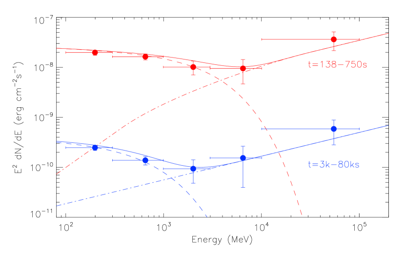
Figure 2.— Fit of the spectrum of LAT emission at two different times. The dashed lines and the dash–dotted lines represent the synchrotron component and the SSC component respectively, and the solid lines represent the sum of them.

4. Discussions

The extended, hard emission above a few GeV, seen in GRB 130427A, represents strong evidence of a SSC component in the forward shock emission. The appearance of the SSC component implies that the circumburst density should not be too low, in contrast to the result in the previous study that the circumburst density of LAT–detected bursts is on average lower than usual (Cenko et al., 2011). The inferred density in this work is of the same order of the typical ISM density in the galaxy disk where massive stars reside.

Recently, Laskar et al. (2013) modeled the low-energy afterglows of this GRB with a forward-reverse shock synchrotron emission model. However, we find that their model predicts a synchrotron flux about one order of magnitude lower than the observed flux in the LAT energy range. To interpret the multi-band afterglow data including the LAT data, we proposed a forward shock synchrotron plus SSC emission scenario. We also find that an ISM environment is favored by the slow decay of 2–100 GeV flux, which is explained as the SSC origin.

We would like to thank He Gao, Zhuo Li and the anonymous referee for valuable suggestions. This work is supported by the 973 program under grant 2009CB824800, the NSFC under grants 11273016, 10973008, and 11033002, the Excellent Youth Foundation of Jiangsu Province (BK2012011), and the Fok Ying Tung Education Foundation. XFW is partially supported by the National Basic Research Program (”973” Program) of China (Grant 2013CB834900), the One-Hundred-Talents Program and the Youth Innovation Promotion Association of the Chinese Academy of Sciences, and the Natural Science Foundation of Jiangsu Province.

References

- Barniol Duran & Kumar (2011) Barniol Duran, R., & Kumar, P. 2011, MNRAS, 412, 522
- Cenko et al. (2011) Cenko, S. B., Frail, D. A., Harrison, F. A., et al. 2011, ApJ, 732, 29
- Evans et al. (2013) Evans, P. A., Page, K. L., Maselli, A., Mangano, V., Capalbi, M., Burrows, D. N. 2013, GCN Circ. 14502
- Fan et al. (2013) Fan, Y.-Z., Tam, P. H. T., Zhang, F.-W., et al. 2013, arXiv:1305.1261
- Flores et al. (2013) Flores, H., Covino, S., Xu, D., et al. 2013, GRB Coordinates Network, 14491, 1
- Goodman (1997) Goodman, J. 1997, New Astronomy, 2, 449
- He et al. (2011) He, H. N., Wu, X. F., Toma, K., Wang, X. Y., & Mészáros, P. 2011, ApJ, 733, 22
- Kann & Schulze (2013) Kann, D. A. & Schulze, S. 2013, GCN Circ. 14580, 1
- von Kienlin (2013) von Kienlin, A. 2013, GRB Coordinates Network, 14473, 1
- Kumar & Barniol Duran (2009) Kumar, P., & Barniol Duran, R. 2009, MNRAS, 400, L75
- Kumar & Barniol Duran (2010) Kumar, P., & Barniol Duran, R. 2010, MNRAS, 409, 226
- Laskar et al. (2013) Laskar, T., Berger, E., Zauderer, B. A., et al. 2013, arXiv:1305.2453
- Lemoine et al. (2013) Lemoine, M., Li, Z., & Wang, X.-Y. 2013, arXiv:1305.3689
- Levan et al. (2013) Levan, A. J., Cenko, S. B., Perley, D. A., & Tanvir, N. R. 2013, GCN, 14455, 1
- Liu & Wang (2011) Liu, R. Y., & Wang, X. Y., 2011, ApJ, 730, 1
- Maxham et al. (2011) Maxham, A., Zhang, B.-B., Zhang, B., 2011, MNRAS, 415, 77
- Piran & Nakar (2010) Piran, T., & Nakar, E. 2010, ApJ, 718, L63
- Sagi & Nakar (2012) Sagi, E., & Nakar, E. 2012, ApJ, 749, 80
- Sari & Piran (1995) Sari, R., & Piran, T. 1995, ApJ, 455, L143
- Sari et al. (1998) Sari, R., Piran, T., & Narayan, R. 1998, ApJ, 497, L17
- Sari & Esin (2001) Sari, R. & Esin, A. A. 2001, ApJ, 548, 787
- Tam et al. (2013) Tam, P.-H. T., Tang, Q.-W., Hou, S.-J., Liu, R.-Y., & Wang, X.-Y. 2013, ApJ, 771, L13
- Trotter et al. (2013) Trotter, A., Reichart, D., Haislip, J., et al. 2013, GRB Coordinates Network, 14510, 1
- Wang et al. (2006) Wang, X.-Y., Li, Z., Mészáros, P. 2006, ApJ, 641, L89
- Wang et al. (2010) Wang, X.-Y., He, H.-N., Li, Z., Wu, X.-F., & Dai, Z.-G. 2010, ApJ, 712, 1232
- Wang et al. (2013) Wang, X.-Y., Liu, R.-Y., & Lemoine, M. 2013, ApJ, 771, L33
- Wijers & Galama (1999) Wijers, R. A. M. J., & Galama, T. J. 1999, ApJ, 523, 177
- Xu et al. (2013a) Xu, D., et al. 2013, GCN Circ. 14478, 1
- Xu et al. (2013b) Xu, D., de Ugarte Postigo, A., Leloudas, G., et al. 2013, arXiv:1305.6832
- Zhang & Mészáros (2001) Zhang, B., & Mészáros, P. 2001, ApJ, 559, 110
- Zhu et al. (2013) Zhu, S., Racusin, J., Kocevski, D., McEnery, J., Longo, F., Chiang, J., & Vianello, G. 2013b, GCN Circ. 14508, 1
- Zou et al. (2009) Zou, Y.-C., Fan, Y.-Z., & Piran, T. 2009, MNRAS, 396, 1163