Stellar orbits and the survival of metallicity gradients in simulated dwarf galaxies

Abstract

We present a detailed analysis of the formation, evolution, and possible longevity of metallicity gradients in simulated dwarf galaxies. Specifically, we investigate the role of potentially orbit-changing processes such as radial stellar migration and dynamical heating in shaping or destroying these gradients. We also consider the influence of the star formation scheme, investigating both the low density star formation threshold of $0.1\,\mathrm{amu\,cm^{-3}}$, which has been in general use in the field, and the much higher threshold of $100~{}\mathrm{cm^{-3}}$, which, together with an extension of the cooling curves below $10^{4}$ K and and increase of the feedback efficiency, has been argued to represent a much more realistic description of star forming regions.

The Nbody-SPH models that we use to self-consistently form and evolve dwarf galaxies in isolation show that, in the absence of significant angular momentum, metallicity gradients are gradually built up during the evolution of the dwarf galaxy, by ever more centrally concentrated star formation adding to the overall gradient. Once formed, they are robust and can easily survive in the absence of external disturbances, with their strength hardly declining over several Gyr, and they agree well with observed metallicity gradients of dwarf galaxies in the Local Group. The underlying orbital displacement of stars is quite limited in our models, being of the order of only fractions of the half light radius over time-spans of 5 to 10 Gyr in all star formation schemes. This is contrary to the strong radial migration found in massive disc galaxies, which is caused by scattering of stars off the corotation resonance of large-scale spiral structures. In the dwarf regime the stellar body only seems to undergo mild dynamical heating, due to the lack of long-lived spiral structures and/or discs.

The density threshold, while having profound influences on the star formation mode of the models, has only an minor influence on the evolution of metallicity gradients. Increasing the threshold 1000-fold causes comparatively stronger dynamical heating of the stellar body due to the increased turbulent gas motions and the scattering of stars off dense gas clouds, but the effect remains very limited in absolute terms.

1 Introduction

Comparing observations to simulations is a powerful approach to studying the physical processes involved in the formation and evolution of galaxies. Dwarf galaxies, in particular, are ideal probes for this. Their low masses and small sizes allow hydrodynamical simulations to reach high spatial resolutions. For the same reasons, they are also very sensitive to the effects of star formation (e.g. supernova explosions), contrary to massive galaxies. And at least the dwarfs within the Local Group can be studied in great depth, thus providing sufficiently detailed data to compare the high resolution simulations to. The results derived from studying dwarf galaxies are of direct relevance to galaxy evolution in general.

Stellar population gradients, i.e. the radial variation of metallicity and age projected along the line of sight, offer direct insights into the past star-formation and metal enrichment histories of galaxies. Observationally, there is an ever growing collection of dwarf galaxies with gradients, found both in the Local Group (Alard 2001; Harbeck et al. 2001; Tolstoy et al. 2004; Battaglia et al. 2006, 2011, 2012; Bernard et al. 2008; Kirby et al. 2011; Kirby, Cohen, & Bellazzini 2012; Monelli et al. 2012) and in nearby galaxy clusters and groups (Koleva et al. 2009; Koleva et al. 2011; Chilingarian 2009; Crnojević, Grebel, & Koch 2010; Lianou, Grebel, & Koch 2010; den Brok et al. 2011). These encompass objects of different masses and star formation modes (spheroidals, ellipticals, star-forming, quiescent, transitional type, …), in different environments (from isolated to densely populated), with different gradient formation histories (slowly built-up gradients, Battaglia et al. 2006, 2012; or already present in the oldest populations, Tolstoy et al. 2004; Bernard et al. 2008; Koleva et al. 2009), which are investigated with different techniques. Likewise, on the theoretical/numerical side, there is a physical foundation for the existence of metallicity gradients in both massive galaxies (Bekki & Shioya, 1999; Hopkins et al., 2009; Pipino et al., 2010, and references therein) and for dwarf galaxies (Valcke et al., 2008; Stinson et al., 2009; Schroyen et al., 2011; Łokas, Kowalczyk, & Kazantzidis, 2012), but see Revaz & Jablonka (2012).

This prompts the question of how and when these gradients are formed and how, once formed, they can be maintained. These are the topics we want to investigate in the current paper. More specifically, we want to address whether radial displacements of stars through orbit-changing processes (such as dynamical heating by scattering of stars or radial stellar migration through interactions with spiral-like structures) play a role in potentially erasing or weakening any pre-existing population gradients in dwarf galaxies.

This paper is structured as follows. We give a description of our numerical models and methods in Section 2, and present the simulations in Section 3. General influences of the model parameters are summarized in Section 4 before going on to the more specific results. In Section 5 we analyse the evolution of the metallicity profiles in our model dwarf galaxies, and compare them to observed metallicity gradients in the Local Group. Section 6 looks into the underlying orbits and kinematics in the stellar body of our simulated dwarf galaxies, and tries to connect these to the findings on metallicity gradients. We summarize and conclude in Section 7.

2 Models and methods

2.1 Codes

For this work, we rely mainly on two codes. Firstly, we use the Nbody-SPH code Gadget-2 (Springel, 2005) for the actual simulating, providing us with snapshots of the model dwarf galaxies - which contain positions, masses and velocities for all particles, and properties specific to stellar and gaseous particles such as ages, metallicities and densities. Secondly, we developed our own in-house analysis tool Hyplot for analysing and visualizing these data files, which is able to calculate any desired physical quantity of the dwarf galaxy model, and also transform them to mimic observational quantities.

2.1.1 Simulation code

The simulation code we use is a modified version of the Nbody-SPH code Gadget-2 (Springel, 2005). To the freely available basic version, which only incorporates gravity and hydrodynamics, we added several astrophysical extensions. These consist of radiative cooling, star formation, feedback processes and chemical enrichment - which altogether give rise to the self-regulating chemical evolution cycle in galaxies. We did not include a cosmic UV background. In order not to add more free parameters to the formalism, we opted not to include a prescription for metal diffusion (Shen, Wadsley, & Stinson, 2010; Gibson et al., 2013). Judging from figure 9 from Shen, Wadsley, & Stinson (2010), the gas enriched by metal diffusion achieves metallicities that are more than an order of magnitude smaller than the “enriching” material. We therefore expect that the inclusion of diffusion would only have a minor effect on our results. More detailed information about the basic implementations of these processes can be found in Valcke et al. (2008); Schroyen et al. (2011), and the relevant modifications we have made to them are described further in this section.

2.1.2 Analysis and visualisation

For the analysis, we used our own Hyplot package, which is freely available on SourceForge. It is an analysis/visualisation tool especially suited for Nbody-SPH simulations (currently only for Gadget-2 datafiles, but easily extensible to any data format), written mainly in Python and C++. PyQT and Matplotlib are used for the GUI and the plotting, and it is also fully scriptable in Python. All analyses, plots and visualisations in this paper have been made using Hyplot.

2.2 Initial conditions

As in Valcke et al. (2008); Schroyen et al. (2011); Cloet-Osselaer et al. (2012), the simulations start at redshift 4.3 from an isolated spherically symmetric initial setup, consisting of a dark matter halo with an initial density profile, and a gas sphere that can be given an initial rotation profile. See Cloet-Osselaer et al. (2012) for a detailed account of the cosmological motivation for our initial conditions. Subsequently, the gas cools, collapses into the gravitational well of the dark matter, and is able to form the stellar body of the galaxy through a self-consistent description of star formation, feedback and metal enrichment.

Stellar feedback alone is unable to unbound the gas from the potential well of the simulated dwarf galaxies so they retain at least part of their gas reservoirs throughout the simulations. In Schroyen et al. (2011), it was shown that high-angular-momentum dwarf galaxies foster continuous star formation and are dwarf-irregular-like while low-angular-momentum dwarf galaxies have long quiescent periods in between star-formation events. During these lulls, these dwarfs would be classified as dwarf spheroidals or dwarf ellipticals (although containing gas for future star formation). We do not aim specifically at simulating either late-type dwarfs or early-type dwarfs: their classification depends on when during their star-formation they are observed, a view which is also advocated in Koleva et al. (2013). Within this unified picture, a meaningful comparison of our simulations with observations of both early-type and late-type dwarf galaxies is possible.

2.2.1 Dark matter halo

The dark matter (DM) halo in our dwarf galaxy models, which is implemented as a “live” halo, serves as the background potential in which the baryonic matter collapses. The density profile is set to a cusped NFW profile (Navarro, Frenk & White, 1996) dark matter halo:

$$\rho_{dm}(r)=\frac{\rho_{s}}{\frac{r}{r_{s}}(1+\frac{r}{r_{s}})^{2}},$$ (1)

with radius $r$ and characteristic parameters $\rho_{s}$ and $r_{s}$ (see Fig. 1). In Cloet-Osselaer et al. (2012) the details of the implementation are discussed, with the difference that instead of using the parameter correlations from Wechsler et al. (2002) and Gentile et al. (2004) we now use those from Strigari et al. (2007), since they are derived specifically for low-mass systems.

It is convincingly shown in Cloet-Osselaer et al. (2012) how the central dark-matter cusp is naturally and quickly flattened through gravitational interactions between dark and baryonic matter:

1. when collapsing into the DM potential well the central density of the gas gradually increases, hereby adiabatically compressing the center of the DM halo

2. when the gas density reaches the threshold for star formation (see Section 2.3), stellar feedback causes a fast removal of gas from the central regions of the DM halo, to which the DM halo responds non-adiabatically by a net lowering of the central density.

A cusped density profile will thus naturally evolve into a more cored density profile if a self-consistent star formation cycle is included in the model, as shown in the inset in Fig. 1.

This flattening effect is seen in all our models, with its strength related to the value of the density threshold (ranging from $\mathrm{0.1~{}to~{}100\,cm^{-3}}$, see 2.3). While this cusp flattening effect has also been found by other authors, such as Governato et al. (2010), its strength and the sizes of the formed cores may vary between authors. This can be explained by the fact that different authors use different star-formation density thresholds and that some, like Governato et al. (2010), select dwarf galaxies from fully cosmological simulations of a larger volume of the universe. The latter type of simulations includes the dwarf galaxies’ full formation and merger history. This is much more disruptive than what we employ here. Our simulations start with an idealized, isolated setup where all the baryonic matter is already present and free to collapse into the DM potential.

2.2.2 Gas sphere

Similar to Revaz et al. (2009) we opted for a pseudo-isothermal density profile for the gas of the form

$$\rho_{g}(r)=\frac{\rho_{c}}{1+\left(\frac{r}{r_{c}}\right)^{2}},$$ (2)

with radius $r$ and the two model parameters $\rho_{c}$ and $r_{c}$, respectively the characteristic density and scale radius. The characteristic density of the gas density profile is related to the characteristic density of the dark matter density profile (see Paragraph 2.2.1) in the following way:

$$\rho_{g,c}=\frac{\Omega_{b}}{\Omega_{dm}}\rho_{dm,c},$$ (3)

where $\rho_{g,c}$ and $\rho_{dm,c}$ are the relevant gas and dark matter densities, respectively, and $\Omega_{b}/\Omega_{dm}=0.2115$ the fraction of baryonic to dark matter (values for the latter taken from the 3-year WMAP results, Spergel et al. 2007). The outer radius of the sphere and the total gas mass contained within it are taken to be the same as in Valcke et al. (2008), which fixes the scale radius $r_{c}$. Fig. 1 shows the initial setup for one of our models.

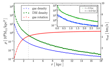
Figure 1: Initial conditions of our dwarf galaxy ’05’ model (Valcke et al., 2008). Several radial profiles are shown: the blue and green are the density profiles of, respectively, the gas and dark matter haloes (left $y$-axis) - red shows the rotational velocity profile of the gas (right $y$-axis). Full lines represent the theoretical curves (found in Paragraphs 2.2.1, 2.2.2, 2.2.3) while markers indicate the actual radial profiles. Inset in the upper right corner shows a zoom-in on the central part of the density profiles, with a higher number of sampling bins (the same units on the axes as the large plot, central part is indicated with a dashed grey line). The dark and light shades of green respectively are the dark matter density profiles at $0$ Gyr and $12.2$ Gyr, showing the flattening of the NFW cusp as in Cloet-Osselaer et al. (2012).

2.2.3 Rotation curves

For the models that are to receive angular momentum, we have chosen an arctangens-shaped initial rotation profile, rising from zero in the center to the maximum value $v_{rot}$ on the edge of the gas sphere (see Fig. 1):

$$v_{tan,i}(r)=\frac{2}{\pi}\arctan\left(\frac{r}{r_{s}}\right)~{}v_{rot},$$ (4)

with radius $r$ and scale radius $r_{s}$. The rotation axis of the galaxy coincides with the $z$-axis, making the latter also the short axis of the galaxy’s oblate stellar body. The $x$ and $y$ axes lie within the galaxy’s equatorial plane.

2.3 Density threshold for star formation

As in many other numerical simulations of galaxy evolution, we allow star formation to occur only if the local gas density exceeds a certain physically motivated threshold. Initially, this threshold was set to the low value of $0.1\,\mathrm{amu\,cm^{-3}}$ (LDT), a value which has been in general use by several authors (e.g. Katz, Weinberg & Hernquist 1996; Stinson et al. 2006; Valcke et al. 2008; Revaz et al. 2009; Schroyen et al. 2011; and references therein). More recently, with numerical resolution following the steady increase of computing power, it has become possible to follow the formation of cold, high-density clouds in which star formation is supposed to occur. Governato et al. (2010), amongst others, therefore advocate using a much higher density threshold of $100~{}\mathrm{cm^{-3}}$ (HDT), which, together with an extension of the cooling curves below $10^{4}$ K, is argued to represent a much more realistic description of star forming regions.

At this high threshold density, the SPH smoothing length, which encompasses about 50-60 gas particles, exceeds the Jeans length down to temperatures of $T_{\rm min}\sim 100$ K. At these high densities and low temperatures, the gravitational softening is larger than both the SPH smoothing and the Jeans lengths and artificial fragmentation is suppressed (softening is set to 30 pc, while the SPH smoothing is typically 8 pc at these densities). Hence, the cold, dense clumps forming in the interstellar medium - with dimensions larger than the gravitational softening scale - are real and they are the cradles of star formation, which is the main aim of the employed star-formation criteria.

In order to produce HDT models which lie on the observed photometric and kinematic scaling relations, an increase of the star-formation density threshold needs to be accompanied by a simultaneous increase in stellar feedback efficiency, in order to counteract the stronger gravitational forces in collapsed areas. This constitutes a fundamental degeneracy in the parameter space of this branch of galaxy modelling, as discussed in Cloet-Osselaer et al. (2012).

In this paper, we wil investigate how the density threshold affects the formation and maintenance of stellar population gradients.

2.4 Cooling curves

As an integral part of the HDT scheme, an extension of the radiative cooling curves for the gas below $10^{4}$ K is necessary. The gas needs to be able to cool further than in LDT models, in order to be able to reach the required density threshold for star formation.

One way of reaching this goal is by supplementing the Sutherland & Dopita (1993) metallicity dependent cooling curves, which are valid for temperatures above $10^{4}$ K, with cooling curves calculated for temperatures below $10^{4}$ K, such as the ones presented by Maio et al. (2007). This is an often used approach in numerical simulations (Sawala et al., 2010; Revaz et al., 2009; Cloet-Osselaer et al., 2012). However, besides the lack of consistency between different cooling curve calculations and the chemical oversimplification of using only metallicity as a compositional parameter, this approach also features an unnaturally sharp drop by about 4 orders of magnitude of the cooling rate at $10^{4}$ K (see Fig. 2). This leads to a pile-up of gas particles at precisely this temperature.

We therefore embarked to produce fully self-consistent radiative cooling curves, featuring a continuous temperature range from 10 K to $10^{9}$ K in one consistent calculation scheme, incorporating all relevant processes and elements. These fit into a larger effort of expanding and improving the physical context of our simulations, which is currently under way: radiative cooling and heating (De Rijcke et al., in preparation); treating gas ionization (Vandenbroucke et al., in preparation). In this paper, however, we will only employ the “first stage” of the improved cooling curves. These not yet take into account any UV background radiation, but they do feature the basis of the new interpolation scheme. Both [Fe/H] and [Mg/Fe] are now used as tracers for estimating, respectively, the contribution of supernovae type Ia and type II to the total composition of the gas. The curves are produced for a range of 8 [Fe/H] values and 6 [Mg/Fe] values, plus a zero metallicity curve, resulting in the 49 continuous cooling curves presented in Fig. 3. This already represents a significant improvement over the chemical composition scheme of Sutherland & Dopita (1993), which at low metallicities only uses SNII abundance ratios (De Rijcke et al., in preparation).

Figure 2: Plot of the first approach for extending the cooling curves below $10^{4}$ K. Right of the dashed grey line are the cooling curves as calculated by Sutherland & Dopita (1993), left are the extensions as calculated by Maio et al. (2007). In simulations these curves are interpolated in temperature and metallicity.

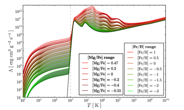
Figure 3: Similar plot as Fig. 2, but now for the “first stage” improved cooling curves. There is no discontinuity anymore around $10^{4}$ K now, due to the consistency in the calculations across the entire temperature range. In simulations these curves are now interpolated in temperature, [Fe/H] and [Mg/Fe], where the latter two respectively encode the contribution of supernovae type Ia and type II to the composition of the gas. Different [Fe/H] are indicated by a colorscale from green to red, while different [Mg/Fe] are indicated through the intensity of the color (colorscale for the latter only shown for the highest [Fe/H]). The black line represents the zero metallicity curve.

3 Simulations

Here we describe the details of the simulation runs that have been performed and used for this research. The methods and theory behind the models are discussed in Section 2, and in Valcke et al. (2008), Schroyen et al. (2011) and Cloet-Osselaer et al. (2012).

We investigate two types of models in this paper. On the one hand, we run simulations according to the prescriptions from our previous research (Schroyen et al., 2011) which employ the, until recently quite standard, low density threshold for star formation and corresponding low feedback efficiency. On the other hand, we also run simulations which feature the specifications discussed in Section 2, such as a high density threshold and a high feedback efficiency. Henceforth, we will refer to them as the low density threshold (LDT) and high density threshold (HDT) models/simulations/runs, respectively.

Several properties of the simulations, however, are shared among the LDT and HDT runs:

• all simulations start with an initial set of 200,000 gas particles and 200,000 dark matter particles.

• initial metallicity is set to $10^{-4}$ solar metallicities.

• initial gas temperature is $10^{4}$ K.

• runtime is approximately $12$ Gyr, starts at redshift 4.3.

• snapshots are made every $5$ Myr, resolving the dynamical timescale.

• the models are isolated.

• the gravitational softening length is 30 pc.

3.1 Low density threshold (LDT) runs

Here, we investigate simulations with initial dark-matter masses of $660\times 10^{6}$ M_⊙ (these runs have labels that end with “05”) and $2476\times 10^{6}$ M_⊙ (these runs have labels that end with “09”). The density threshold is set to $0.1~{}\mathrm{cm^{-3}}$, with a feedback efficiency of 0.1 (i.e. 10 % of the supernova energy is absorbed by the interstellar medium), and cooling curves that do not go below $10^{4}$ K. Simulations with and without rotation have been performed. Rotation was induced by adding a constant rotational velocity of $v_{\rm rot}=5$ km s^-1 to the gas particles. These simulations are basically high time resolution reruns of some of our older models and will serve as a “reference sample” to compare with the new models. The details of these 4 simulations can be found in Table 1.

Table 1: Details of the LDT runs, re-run from Schroyen et al. (2011) (corresponding simulation number in this previous work shown in brackets, further details on the models can also be found there). All quantities are evaluated at the end of the simulation, except for the initial values indicated with index ‘i’. Rows: (1) initial gas mass [$10^{6}\mathrm{M_{\odot}}$], (2) dark matter mass [$10^{6}\mathrm{M_{\odot}}$], (3) stellar mass [$10^{6}\mathrm{M_{\odot}}$], (4) half-light radius [kpc], (5) luminosity-weighted metallicity (B-band), (6)(7) B-band and V-band magnitude, (8) initial rotation speed of gas [km/s].

	LDT05	LDT09	LDTrot05	LDTrot09
	(205)	(209)	(225)	(229)
$M_{g,i}$	140	524	140	524
$M_{dm}$	660	2476	660	2476
$M_{st}$	18.93	468.57	14.35	325.33
$R_{e}$	0.43	0.39	0.63	1.36
$[Fe/H]$	-0.717	-0.053	-0.672	-0.281
$M_{B}$	-11.87	-14.87	-12.2	-15.02
$M_{V}$	-12.51	-15.62	-12.7	-15.62
$v_{i}$	0		5

3.2 High density threshold (HDT) runs

Simulations have also been performed that employ the HDT models as described in Section 2. Again we use a lower mass and a higher mass model, with the same initial masses as the LDT runs in 3.2, again one rotating and one non-rotating. The density threshold for star formation is now set to $100~{}\mathrm{cm^{-3}}$ and employs the first stage novel cooling curves as described in Paragraph 2.4, which span a temperature range from 10 K to $10^{9}$ K (and are extended to $10^{10}$ K with a Bremsstrahlung approximation). The feedback efficiency has been increased to $0.7$, following the results of Cloet-Osselaer et al. (2012) (see Section 2.3). On top of the NFW dark matter halo is placed a pseudo-isothermal gas sphere, which in the rotating models is given an arctangens radial rotation profile, as in 2.2.3, with a $v_{\rm rot}$ of $5$km/s and $r_{s}=1$ kpc. Further details are found in Table 2.

Table 2: Details of the new HDT runs. All values in the first block refer to the initial conditions, the other values (besides those indexed with ‘i’) are final values. Rows: (1) initial gas mass [$10^{6}\mathrm{M_{\odot}}$], (2)(3)(4) characteristics of pseudo-isothermal sphere: density [$10^{7}\mathrm{M_{\odot}/kpc^{3}}$] - scale radius [kpc] - cutoff radius [kpc], (5) dark matter mass [$10^{6}\mathrm{M_{\odot}}$], (6)(7)(8) characteristics of NFW halo: density [$10^{7}\mathrm{M_{\odot}/kpc^{3}}$] - scale radius [kpc] - cutoff radius [kpc], (9) stellar mass [$10^{6}\mathrm{M_{\odot}}$], (10) half-light radius [kpc], (11) luminosity-weighted metallicity (B-band), (12)(13) B-band and V-band magnitude, (14) initial rotation speed of gas [km/s].

	HDT05	HDT09	HDTrot05	HDTrot09
$M_{g,i}$	140	524	140	524
$\rho_{pseudo-iso}$	1.102	0.896	1.102	0.896
$r_{pseudo-iso}$	0.234	0.403	0.234	0.403
$r_{g,max}$	18.894	29.353	18.894	29.353
$M_{dm}$	660	2476	660	2476
$\rho_{nfw}$	5.211	4.236	5.211	4.236
$r_{nfw}$	0.744	1.251	0.744	1.251
$r_{dm,max}$	21.742	33.634	21.742	33.634
$M_{st}$	2.37	32.19	1.58	52.813
$R_{e}$	0.23	0.58	0.22	1.06
$[Fe/H]$	-0.98	-0.834	-0.922	-0.736
$M_{B}$	-9.69	-12.79	-9.69	-13.44
$M_{V}$	-10.3	-13.34	-10.24	-13.98
$v_{i}$	0		5

3.3 Truncated simulations

For each of the abovementioned non-rotating simulations we also run a “truncated” version, where the star formation is shut off at a specific time during the evolution. This allows us to assess most clearly whether any population gradients present at the moment of truncation can persist for an extended period.

The truncation can be done in two ways:

1. The star formation routines are shut off at a certain time, which for the HDT simulations also requires shutting off cooling below $10^{4}$ K because otherwise the gas quickly becomes extremely dense, causing the code to crash. The gas remains present, but becomes inert, the “gastrophysics” are switched off.

2. All gas particles are removed from the simulation, without changing the physics. This is basically a poor man’s version of ram-pressure-stripping, mimicking a dwarf galaxy that is stripped of its gas on short timescales by the intergalactic medium.

We opted for the second option, since it stops star formation in a more “natural” way, without tinkering with the physics and switching certain processes off. In practice we take a certain snapshot of the existing simulations, remove the gas particles from it, and use it as the initial condition for a simulation that restarts at the moment of truncation. We have chosen the simulations to be truncated at 8 Gyr, allowing us to study the stability of any existing population gradients over periods of time of the order of 4 billion years.

4 LDT vs. HDT

Several differences in the physical features of the LDT and HDT simulations are worth highlighting here, before going on to the specific research results in the next sections.

The principal feature of the HDT models is obviously the formation of dense and cold clumps in the gas in which star particles form (Governato et al., 2010). In Fig. 2, the difference in gas structure between the LDT and the HDT simulation is apparent. Whereas in the LDT case the gas is quite “fuzzy”, and collectively above the density threshold in a large area, in the HDT case it is much more structured and fragmented in dense clumps, with only localized individual density peaks reaching above the density threshold.

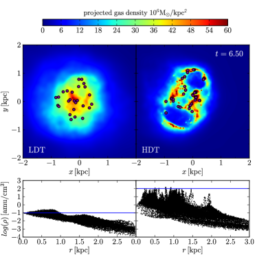
Figure 4: The top row shows rendered images of a LDT (left) and HDT (right) model. Superimposed on the color coded (projected) gas density as purple dots are the newly formed stars, of ages 10 Myr and below. The bottom row shows density-radius scatter plots of the gas particles, with a horizontal blue line indicating the density threshold for star formation in the respective star formation schemes. Note: the left rendered LDT image has actually been generated according to a color scale with values scaled down with a factor 1/10, since otherwise none of the gas would get out of the dark blue range. A full animation of this figure can be found online

This distinction has immediate consequences for the star formation mode, as can be seen in Fig. 5. The non-rotating LDT models show clear star formation episodes of about 2 Gyr long with intermittent lulls of a Gyr or so, with an inwards shrinking of the SF area between episodes and within each episode. The HDT models show much shorter star formation bursts in faster sequention with no shrinking within an episode, but still with a shrinking of the SF area over time between episodes. We can see this change in star formation timescale clearly in the Fourier transform of the star formation rate over time in Fig. 6. The LDT model shows a peak at a period of 3 Gyr, which agrees well with the very noticeable 4 star formation episodes in 12 Gyr seen in Fig. 5, while the HDT model shows a clear shift to shorter periods, with 2 peak values at periods of 0.2 and 0.5 Gyr. These match, respectively, with the sequence of star formation events seen in Fig. 5 in the first 2-3 Gyr and the last 6-7 Gyr.

In Fig. 7, we show the evolution of a HDT model during a single short-duration star-formation event. The event starts when several high-density peaks inside the already dense inner 1 kpc of the galaxy start forming stars. Supernova feedback quickly disrupts the individual star-forming clouds while triggering secondary star formation throughout this dense inner region of the galaxy. Subsequently accumulating feedback evacuates the dense central region about 30-40 Myr after the start of the event, limiting star formation to condensations on the edges of the expanding supernova-blown bubbles until it finally peters out after about 150 Myr. The insets present a zoom on the star-formation event in Fig. 5, which shows this rapidly outward evolution by a slight tilt to the right of the corresponding “plume” of the burst. This chain of events is reminiscent of the “flickering star formation” observed in real dwarf galaxies with bursty star-formation histories (McQuinn et al., 2010). A full animation of the simulated star burst event depicted in Fig. 7 can be found online.

As already concluded by Schroyen et al. (2011), angular momentum smears out star formation in time and space, making the major star-formation events less conspicuous (Fig. 5).

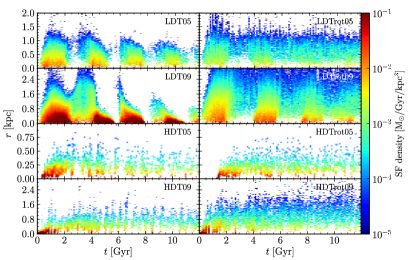
Figure 5: The star formation density (in $\mathrm{M_{\odot}/Gyr/kpc^{3}}$, color coded according to the color scale) plotted in function of time ($x$-axis) and spatial extent (radius, $y$-axis). The non-rotating models are in the left column, the rotating ones in the right column. The four upper plots show the LDT models, the four bottom models show the HDT models.

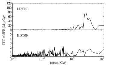
Figure 6: Fourier transform of the star formation rate in function of time, shown as a function of the period of the mode on the $x$-axis.

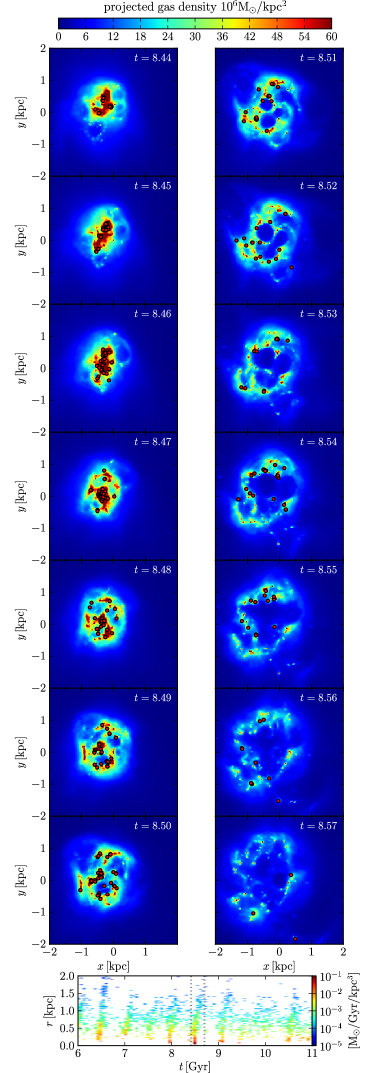
Figure 7: A high time resolution sequence of snapshots capturing a single star-formation event in a HDT model. Red dots indicate newly born star particles. Below is a zoom of the SF density (Fig. 5), with the dotted lines indicating the time range shown.

Moreover, the HDT models produce significantly less stellar mass for the same initial gas mass. However, since all other properties also scale accordingly, the models remain in good agreement with the fundamental observational characteristics: they simply shift along the observed photometric and kinematical scaling relations (Cloet-Osselaer et al., 2012).

5 Metallicity profiles

In this section we present and discuss the evolution of the radial stellar metallicity profiles throughout the simulations, and compare them qualitatively and quantitatively to observed metallicity gradients of dwarf galaxies in the Local Group. As discussed in Section 3 we discern between the LDT/HDT scheme, low/high total mass, and rotating/non-rotating models. Furthermore, for all of the non-rotating models we also present the results from so-called “truncated simulations”, where the star formation is shut off at a specific time during the run. In all cases we consider both the luminosity-weighted and mass-weighted metallicity - the former being the quantity which mimics what is generally measured from observations, while the latter reflects the actual physical distribution of metals.

The way of constructing the profiles from the star particles in our simulations tries to mimic an observational configuration. We choose our “line of sight” along the $y$-axis and make bins along the $x$-axis, mimicking a long-slit spectroscopic observation with the slit aligned along the galaxy’s major axis. In the $z$ direction we restrict the particles to the range $-0.2~{}\mathrm{kpc}\leq z\leq 0.2~{}\mathrm{kpc}$. To reduce numerical scatter and give a clearer picture, we “stack” the profiles in space and time. We use the same procedure as before, now projecting along $x$ and binning $y$, and fold all 4 profiles ($x$ and $y$ axes, both in positive and negative direction) onto one profile of metallicity in function of projected distance to the center. Furthermore, we stack subsequent profiles in time, covering an interval of the order of the dynamical timescale ($\sim 50\mathrm{Myr}$). Adaptive binning is used at the end of the procedure, to avoid erratic values at the edges of the profiles.

Luminosity weighting is done by multiplying the iron (Fe) and magnesium (Mg) masses of a stellar particle with its B-band luminosity value, which is obtained by interpolating in age and metallicity on the MILES population synthesis data (Vazdekis et al., 1996). When summing over the particles in a bin, the total metal masses of the bin are then divided by the total B-band luminosity of the bin.

5.1 LDT sims

Figures 8 and 9 show the evolution of, respectively, the luminosity-weighted and mass-weighted metallicity profiles in the LDT simulations (Table 1).

In the non-rotating cases on the one hand, on the top row of the figures, negative metallicity gradients can be seen to gradually build up inside a radius of $\sim 2$ half-light radii during the model’s evolution. This is due to the centrally concentrated, episodic star formation, which is confined to progressively smaller areas over time (see Section 4 and Schroyen et al. 2011), adding to the overall gradient. The more massive model on the top right plot, however, shows a temporary positive metallicity gradient in its outskirts between 3 and 4 Gyr, which is caused by a star formation episode that starts at larger radii and moves inward (see Fig. 5). A central negative gradient is quickly restored once the star formation reaches the center, and remains stable - except for aging/reddening of the stars which affects the luminosity weighted values (compare Fig. 8 to 9).

The rotating models on the other hand, on the bottom row of the figures, show metallicity profiles which are flat throughout practically the whole evolution, out to well past their half-light radius. As shown in Schroyen et al. (2011), the presence of angular momentum smears out SF in space and time, leading to a chemically more homogeneous galactic body.

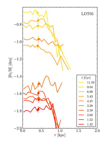
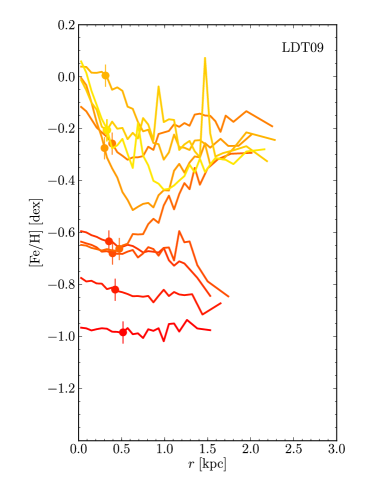
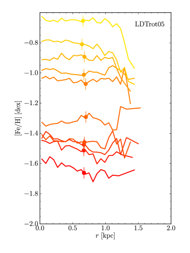
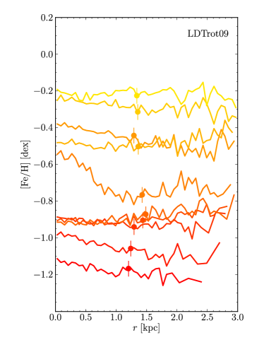
Figure 8: Luminosity-weighted (B-band) metallicity profiles of the LDT models. Evolution throughout the simulation is shown at logarithmic intervals of time, with $0.11$ dex separation - the legend in the top left plot shows the times. The left column shows the low-mass (05) models, the right column shows the high-mass (09) models (see Table 1). Non-rotating models are on the top row, rotating models on the bottom row. The metal contribution of each star particle is weighted by its luminosity in the B-band, to mimick the actual observed quantities. The vertical line symbol on each profile indicates the half-light radius of the dwarf galaxy model at that time.

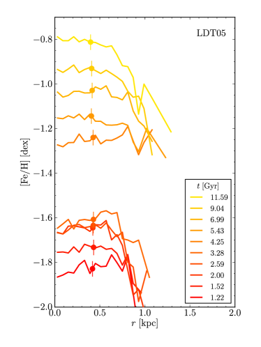
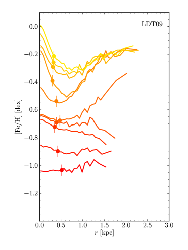
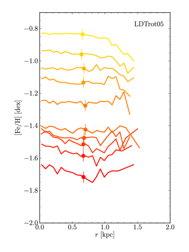
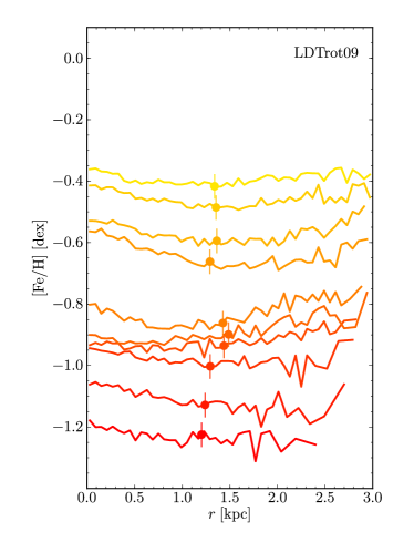
Figure 9: Mass-weighted metallicity profiles of the LDT models. Plot configuration as in Fig. 8. Here, the metal contribution of each star particle is weighted by its mass instead of its luminosity, and therefore the young population does not have the potential to dominate the measurements. This quantity is not what is actually observed, but it gives a better view of the true physical distribution of metals.

5.1.1 Truncated LDT sims

We truncated the star formation around 8 Gyr into the simulation. By then, clear metallicity gradients have built up in all non-rotating simulations. Furthermore, since the model galaxies have already used up or dispersed a substantial amount of their gas when forming stars, the effect of sudden removal of all gas on their structure should be limited.

Figure 10 shows the evolution of the luminosity- and mass-weighted metallicity profiles in the truncated LDT simulations. The luminosity-weighted gradients noticeably diminish over time - or rather, it is mostly the central metallicity that is dropping - but when looking at the mass-weighted profiles it appears that there is hardly any evolution in the physical distribution of metals. The latter can be said to get just slightly shallower over a time span of 4 Gyr, and even the gas removal seems to barely have an effect (the $\mathrm{R_{e}}$ only slightly increases in the first few timesteps).

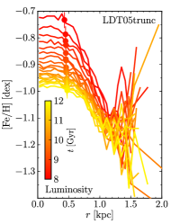
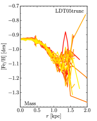
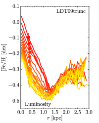
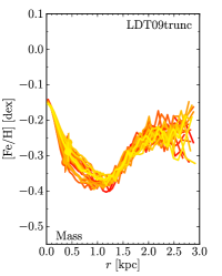
Figure 10: Metallicity profiles of the truncated LDT sims. The respective model and weighting method is indicated on the plot. The time is color coded according to the color bar in the leftmost plot.

5.2 HDT sims

Figures 11 and 12 show the evolution of, respectively, the luminosity-weighted and mass-weighted metallicity profiles in the HDT simulations (Table 2).

Though the SF timescale is now much shorter (Section 4), there still is a general shrinking of the SF area over time, and an overall centrally concentrated star formation - leading to the gradual buildup of negative metallicity gradients in the non-rotating HDT models. The high-mass model features a gradient in its stellar body throughout its entire evolution, while in the low-mass model it is in place from around 5 Gyr onwards. The apparent positive (mass-weighted) gradients during the first few Gyr of the latter, are partly caused by mass recentering difficulties on an initially low number of (stochastically generated) stellar particles, and the stochastic nature of our models in general.

The rotating models show flat(ter) metallicity profiles throughout their evolution, again explained by the spatially and temporally smeared out star formation seen in Fig. 5. For the low-mass model, however, the flattening is not as strong as in the LDT case, but the general difference in behaviour with the non-rotating model is still noticeable. This less pronounced effect is due to the different initial rotation curves (which go to zero in the center, Section 2.2.3, instead of being constant), and the fact that the HDT scheme produces smaller galaxies (Section 4), causing the models to receive less initial angular momentum overall.

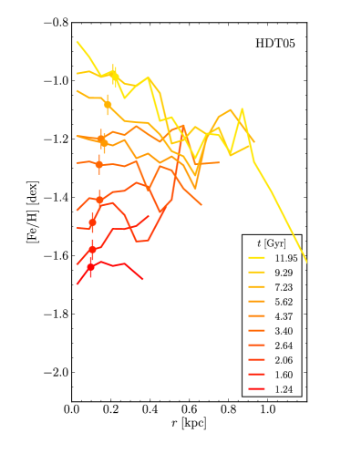
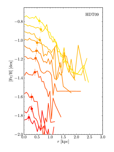
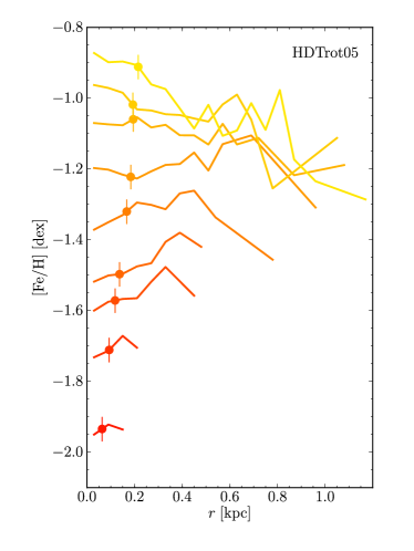
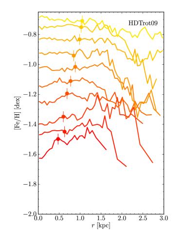
Figure 11: Luminosity-weighted (B-band) metallicity profiles of the HDT models. Plot setup similar to Fig. 8, the simulations can be found in Table 2.

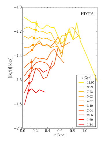
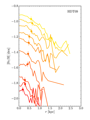
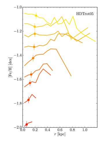
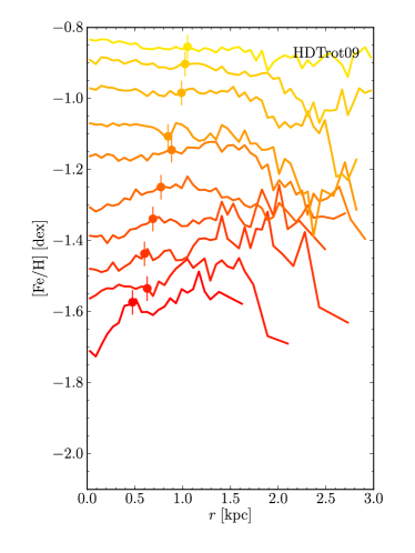
Figure 12: Mass-weighted metallicity profiles of the HDT models. Plot setup similar to Fig. 9.

5.2.1 Truncated HDT sims

As in the LDT sims, the truncation time has been chosen to be around 8 Gyr. And similarly, in Fig. 13 the luminosity-weighted profiles can be seen to diminish noticeably (but survive), while the mass-weighted profiles are much more stable. It should be noted that the latter vary more significantly than in the LDT models, meaning the physical distribution of metals changes more, but in absolute terms this is still very limited. The evolution of the half-light radius in the first few timesteps also shows that the gas removal has a bigger effect here, because of the larger amount of gas present in the central regions (due to higher densities and less gas used) which is suddenly removed.

The HDT05trunc profiles are particularly noisy, due to the relatively low number of particles that is actually used for generating the profile. The stellar mass is very low to begin with (see Table 2, which shows the value at 12 Gyr), and additionally, the method used to generate the profiles excludes a large part of these stellar particles (see beginning of this section).

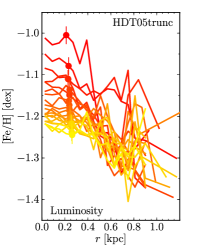
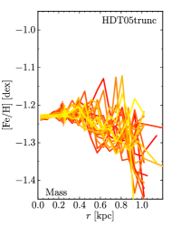
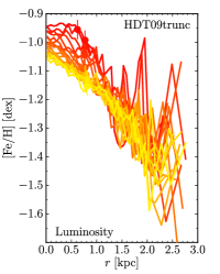
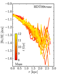
Figure 13: Metallicity profiles of the truncated HDT sims. Similar to Fig. 10. Color bar is in the rightmost plot.

5.3 General conclusions on metallicity gradients

The basic findings on metallicity gradients and the mechanism behind their evolution from Schroyen et al. (2011) hold true in the LDT and HDT schemes.

The general conclusions about the evolution of metallicity gradients in our non-rotating dwarf galaxy models are that

• metallicity gradients are gradually built up during the evolution of the dwarf galaxy, by centrally concentrated star formation which additionally gets limited to smaller areas over time, progressively adding to the overall metallicity gradient.

• formed metallicity gradients seem to be robust, and able to survive over several Gyr, without significantly changing the physical distribution of metals.

All this strongly speaks against the possibility of erasing metallicity gradients in dwarf galaxies without an external disturbance, since even our most realistic (HDT) models do not show any significant decline in the gradients.

5.3.1 Comparison to observed metallicity gradients

We can compare the stellar metallicity gradients in our model dwarf galaxies with observed stellar metallicity gradients from dwarf galaxies in the Local Group, with the aid of Fig. 14 and Table 3. We selected 7 dwarf galaxies from the Local Group, for which the literature provides data on their metallicity gradients that extend far enough outward (several times their half-light radius). These galaxies (and corresponding references) are: Sculptor (Tolstoy et al., 2004); Fornax (Battaglia et al., 2006); Sextans (Battaglia et al., 2011); LeoI, LeoII, Draco (Kirby et al., 2011); VV124 (Kirby, Cohen, & Bellazzini, 2012). Structural parameters for these object were taken from the table that Łokas, Kazantzidis, & Mayer (2011) compiled from the literature, which were (for the objects of interest here) mostly obtained from Mateo (1998) and Walker et al. (2010).

Figure 14 shows the metallicity gradients from the observed dwarf galaxies, where the radial distance is expressed in, respectively, kiloparsec and $R_{e}$. A line is fit to the data points within $3\,R_{e}$, the slope of which is in brackets in the legend of the figure and in Table 3. This collection of objects displays a wide variety in absolute metallicities, slopes, and profile shapes, as do the models:

• Steep, sharply peaked metallicity profiles with a possible increase or “bump” at larger radii (VV124, Sculptor), which is comparable to the metallicity profile of the LDT09 model (Fig. 8, top right, yellow curve). As in the simulations, this bump could indicate a significant star formation episode in the past that mainly took place in the outer regions of the dwarf galaxy, and temporarily enriched these regions more than the inner regions. The central metallicity peak is likely connected to these dwarf galaxies/models being more centrally concentrated.

• Metallicity profiles that show much less or almost no gradient within their $R_{e}$, but get steeper at larger radii (LeoII, Draco), as is the case in the LDT05 and HDT09 model (respectively top left of Fig. 8 and top right of Fig. 11, yellow curves).

• Steadily decreasing, almost linear metallicity profiles over their entire range (Fornax, Sextans, LeoI), similar to the HDT05 model (Fig. 11, top left, yellow curve).

Table 3 lists the slopes of the metallicity profiles in both the observations and the simulations, which have all been calculated in the same way. The simulated dwarf galaxies, which are set up from only two different mass models, show slopes between -0.3 and -0.6 dex per kpc (-0.13 and -0.23 dex per $R_{e}$). The observed dwarf galaxies, that boast a wider range of masses, show slopes between -0.25 and -1.1 dex per kpc (-0.05 and -0.25 dex per $R_{e}$).

Both in shapes and slopes the metallicity profiles of our dwarf galaxy models fall well within the observed range of metallicity profiles. In terms of absolute metallicity values the models are located on the high end of the observed range, which is due to the models generally being more massive than the observed galaxies. The values for the HDT models lie around those of Fornax and VV124, while the values for the LDT models however lie significantly higher, which is in agreement with what a comparison of the dynamical masses of the observed and simulated galaxies would imply (as discussed in Section 4, the LDT scheme shifts the galaxy models along the scaling relations towards higher stellar masses compared to the HDT scheme).

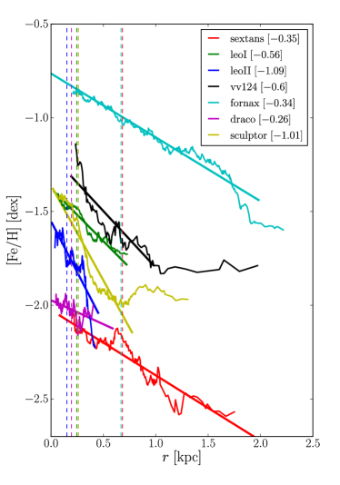
Figure 14: Observed radial stellar metallicity profiles of 7 Local Group dwarf galaxies, in function of radius in kpc. The slopes of the linear fits to these gradients are indicated in brackets in the legend of the figure, and are expressed in dex/kpc. Dashed vertical lines indicate the half-light radii of the galaxies.

Table 3: Columns: (1) dynamical mass calculated as $167\beta R_{e}\sigma_{c}^{2}$, with $\beta=8$ and $\sigma_{c}$ the central velocity dispersion [$10^{6}\mathrm{M_{\odot}}$], (2) V-band magnitude, (3) half-light radius [kpc], (4) central velocity dispersion [km/s], (5) ratio of V over velocity dispersion, (6) metallicity [dex], (7)(8) slope of metallicity profile. Sources: (1) and (6) use data from Mateo (1998), (2), (3) and (5) use data from Łokas, Kazantzidis, & Mayer (2011), (4) uses data from Walker et al. (2010). All data for VV124 comes from Kirby, Cohen, & Bellazzini (2012) except $M_{V}$ and $V/\sigma$ from Łokas, Kazantzidis, & Mayer (2011).

name	mass	$M_{V}$	$R_{e}$	$\sigma_{c}$	$V/\sigma$	[Fe/H]	$\Delta$[Fe/H]	$\Delta$[Fe/H]
	[$10^{6}M_{\odot}$]	[mag]	[kpc]	[km/s]		[dex]	[dex/kpc]	[dex/$R_{e}$]
Sculptor	15.1	-10.53	0.260	9.2	0.3	-1.8	-1.01	-0.26
Fornax	98.7	-13.03	0.668	11.7	0.18	-1.3	-0.34	-0.23
Sextans	38.7	-9.20	0.682	7.9	0.48	-1.7	-0.35	-0.24
LeoI	25.2	-11.49	0.246	9.2	0.33	-1.5	-0.56	-0.14
LeoII	9.2	-9.60	0.151	6.6	0.28	-1.9	-1.09	-0.16
Draco	24.0	-8.74	0.196	9.1	0.21	-2.0	-0.26	-0.05
VV124	19.5	-12.40	0.260	9.4	0.45	-1.14	-0.60	-0.16
LDT05	260	-12.51	0.430	21.3	0.18	-0.717	-0.54	-0.23
LDT09	1090	-15.62	0.391	45.7	0.03	-0.053	-0.39	-0.15
HDT05	18.2	-10.30	0.224	7.8	0.08	-0.98	-0.57	-0.13
HDT09	147	-13.34	0.588	13.7	0.57	-0.834	-0.35	-0.20
LDTrot05	200	-12.7	0.630	15.4	1.45	-0.672	-0.02	-0.01
LDTrot09	1013	-15.62	1.361	23.6	1.86	-0.281	0.01	0.02
HDTrot05	16.7	-10.24	0.217	7.6	0.95	-0.922	-0.31	-0.07
HDTrot09	278	-13.98	1.062	14.0	1.64	-0.736	-0.03	-0.03

6 Stellar orbits and kinematics

This section is devoted to a more detailed analysis of the stellar particles and their orbits and kinematics in our models. We want to have a measure of how strongly the stellar particles actually move away from their original orbits, to have an idea what is actually happening with them throughout the evolution of the models, and see if this could justify stable stellar metallicity gradients. We do this by looking at the stellar velocity dispersions of different populations in Fig. 19 and at the orbital displacements of the stellar particles with respect to the mean radius of their orbits at their time of birth in Fig. 15, 16, 17, and 18.

As mentioned in Section 3, snapshots are made every $5$ Myr, which is sufficient to resolve each particle’s orbit in detail. The evolution of a stellar particle’s radius during the course of the whole simulation is then re-binned in the time dimension to bins of 1 Gyr wide, so that effectively each bin gives the average value of the stellar particle’s radius over several of its orbits. Next, for both radius and time the averaged “birth” values are subtracted, and for each time bin the average (along with several percentiles) is taken over all available stellar particles. This gives us a visualization of the statistical deviation from the original mean orbital radius of the star particles in our models, in function of time since their birth. In our simulations we looked at this statistical deviation of both the absolute difference in mean orbital radius (Fig. 15 and 16), and the actual, signed, difference in mean orbital radius (Fig. 17 and 18). The former will give a clearer picture of how strongly the stellar particles move away from their original mean orbital radius, the latter will indicate the preferred direction (inward or outward). For all simulations, only the orbits of a randomly chosen 15 to 25 percent of the stellar particles are extracted from the data snapshots, to keep the amount of files manageable. Particles outside of a radius of $5\times\mathrm{R_{e}}$ are not considered, since they are in number not important for the metallicity gradients, but could have a disproportionately large influence on the average values of deviation, because they can move about easier at the edge of the potential well. Finally, if a time bin has less than half of the average amount of orbits of the previous time bins, the time bin is removed (and subsequently all that come after that as well), to ensure the amount of stellar particles on which the statistics are done does not become too low.

6.1 LDT sims

Figure 15 and 17 show, respectively, the “absolute” and “signed” radial orbital displacements in our LDT models.

From Fig. 15 it is immediately apparent that the orbital displacement in these models is very limited, to just fractions of about 0.1 to 0.3 of the $\mathrm{R_{e}}$, on average, over the lifetime of the simulated dwarf galaxy. Several trends are also noticeable here, :

• More massive models feature more displacement, caused by more turbulence and a higher velocity dispersion (properties which are set by the mass of the galaxy as the main parameter - see Table 3 and Stinson et al. 2007; Valcke et al. 2008; Schroyen et al. 2011).

• Rotating models feature less displacement compared to non-rotating models with the same mass. The presence of angular momentum - and so, ordered motions in the stellar body gaining importance over the random motions/turbulence - causes a lower velocity dispersion, as can be seen in Table 3 and figure 13 of Schroyen et al. (2011).

• The lowering effect of angular momentum gets stronger with increasing mass, as evidenced by the fact that the more massive LDTrot09 model shows a slightly lower stellar migration than the LDTrot05 model. This is because, in higher mass galaxies, ordered motions (if they are present) are inherently more important than the random motions, compared to lower mass galaxies. Or in the other direction: the lower the galaxy mass, the more dominant random motions/turbulence become over ordered motions (Kaufmann, Wheeler, & Bullock, 2007; Roychowdhury et al., 2010; Sánchez-Janssen, Méndez-Abreu, & Aguerri, 2010; Schroyen et al., 2011).

In Fig. 19, top panel, no clear trends can be seen in the velocity dispersion over different populations of stars. The only noticeable property is a possible slight increasing of the dispersion in all models for the youngest stellar populations, which can be interpreted as the effect that the (relatively strong) star formation of the model starts having on its own potential.

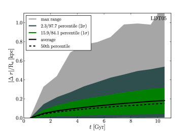
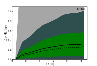
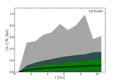
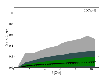
Figure 15: Radial stellar orbital displacements in the LDT models, visualised by the “absolute” statistical deviation from the birth radius, in function of time since birth (as explained in Section 6). Radius is expressed in function of $\mathrm{R_{e}}$. The grey zone marks the maximum range, while the light and darker green respectively represent the 15.9/84.1 and 2.3/97.7 percentile regions (corresponding to 1$\sigma$ and 2$\sigma$ if the underlying distribution were Gaussian). The dotted and full line show the 50th percentile and the average.

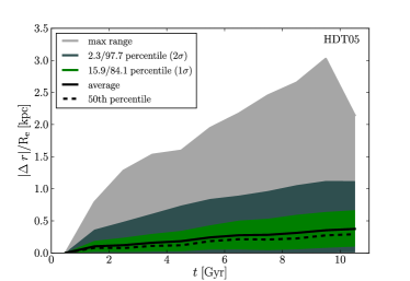
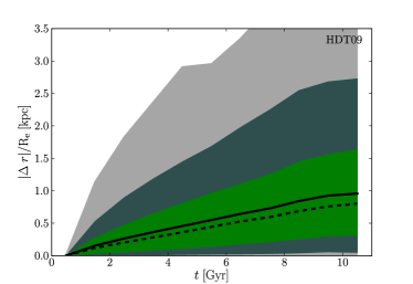
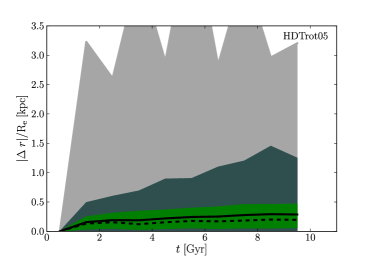
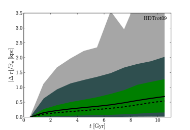
Figure 16: Radial stellar orbital displacement in the HDT models. Figure identical to Fig. 15.

6.2 HDT sims

Figures 16 and 18 show, respectively, the “absolute” and “signed” orbital displacements in the HDT models.

From Fig. 16 we can see that in the HDT models the radial orbital displacement is substantially larger than in the LDT models - roughly 3 times larger. But still this means only fractions of the $\mathrm{R_{e}}$, on average, over timespans of several Gyr (e.g. 0.2 to 0.5 $\mathrm{R_{e}}$ over 5 Gyr), and in the most massive model reaching values of the order of the $\mathrm{R_{e}}$ only over the entire lifespan of the simulated dwarf galaxy. Most of the trends identified in the LDT models in 6.1 appear valid here as well: adding mass increases the radial diffusion, while adding angular momentum lowers it - although the latter to a slightly lesser extent than in the LDT models, due to the different rotation curves (Section 2.2.3) that deliver less angular momentum to the central gas. This can be seen in the behaviour of the velocity dispersion in Table 3 and Fig. 19, bottom frame: there is a clear difference between the dispersions of models with different mass, but virtually no difference between models with the same mass but different angular momenta - contrary to the situation in the top frame for the LDT models.

Figure 18 shows that in the gradient-producing non-rotating HDT models, stellar particles tend to move significantly outward against the gradient. This is contrary to what is observed in their LDT counterparts, which show both inward and outward stellar diffusion (see Fig. 17). There is also an “equalizing” effect seen here, where rotation decreases this outward tendency, though the less massive HDTrot05 model is the only one which comes anywhere close to showing symmetric (equal inward and outward) radial orbital displacements.

In Fig. 19, bottom panel, there is now a trend to be seen in the velocity dispersion of the HDT models over different stellar populations: older populations clearly have larger velocity dispersions than younger populations.

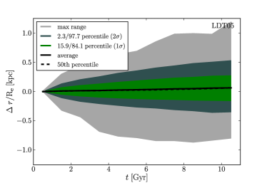
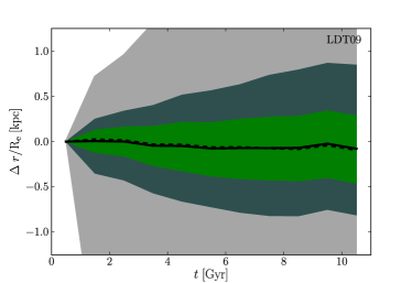
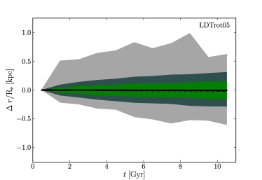
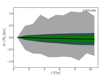
Figure 17: Radial stellar orbital displacement in the LDT models, here in positive or negative distance from the birth radius of the star. Other properties of the plots identical to Fig. 15.

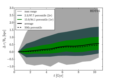
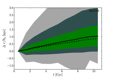
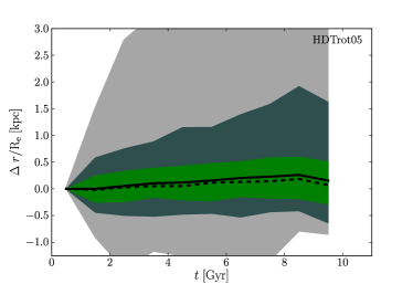
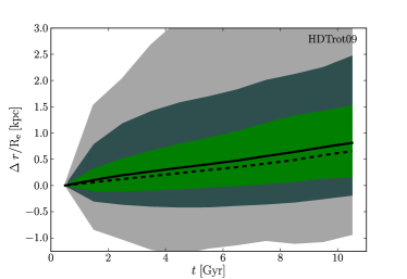
Figure 18: Radial stellar orbital displacement in the HDT models. Figure identical to Fig. 17.

6.3 General conclusions on stellar orbits

The general conclusion here is that radial orbital displacements of stellar particles are limited in our dwarf galaxy models, being generally measured in fractions of the half light radius over time spans of 5 to 10 Gyr. This qualitative statement is true, independent of the employed star-formation scheme. This gives us a more solid foundation for the results concerning the stability of metallicity gradients.

Since this is the case for dwarf galaxy models with either low or high angular momenta, this strongly indicates that there are no radically orbit-changing processes at work in dwarf galaxies like there are in bigger galaxies. In massive spiral galaxies there is the so-called “radial stellar migration”, which is caused by gravitational interactions between individual stars and the large-scale spiral structures rotating in the stellar and gaseous discs that drive stars away from the corotation radius (Sellwood & Binney, 2002; Roškar et al., 2008, 2012). This is able to move stars about over large radial distances while maintaining quasi-circular orbits, and it seems the evidence, both theoretical and observational, is building up for this being an effect of broad importance in disc galaxy evolution : it plays a fundamental role in the forming of thick discs, (Schönrich & Binney, 2009; Loebman et al., 2011), the distribution of stellar populations, (Roškar et al., 2008), and has evidently strong implications for the forming/survival of metallicity gradients (Lépine, Acharova, & Mishurov, 2003). None of our models show an appreciable disk or spiral structures in their stellar body, because it is generally too thick, dynamically too warm, and influenced by the random motions of the gas in the low mass regime that we are investigating here (Kaufmann, Wheeler, & Bullock, 2007; Roychowdhury et al., 2010; Sánchez-Janssen, Méndez-Abreu, & Aguerri, 2010). Only the rotating dwarfs feature a somewhat flattened stellar body and fast-transient spiral structures in their gas distribution, but these structures are produced by outwardly expanding supernova-blown bubbles being deformed by shear, which are too short-lived and fade away too quickly to have any impact on the stellar dynamics of the models. What - if anything - is happening with the orbits in these dwarf galaxy models is most likely linked to the much more gentle effect of “dynamical heating”, that changes stellar orbits in a more gradual manner. It was already suggested by Spitzer & Schwarzschild (1953) that, for instance, massive gas clouds could have a noticeable influence on the random velocities of stellar orbits.

Quantitatively, the star formation criteria do play a role, however. The HDT models show noticeably more stellar diffusion than the LDT models, who barely undergo any orbital displacement at all over their entire simulation time. This increased diffusion is also more strongly aimed outward - agains the gradient - though it is still limited in absolute terms. Two likely causes are the more turbulent character of the gas in general (which is adopted by the stellar body), and the increased scattering of stellar particles off dense gas clumps. Both effects are expected to become more important when the density threshold for star formation increases, and will therefore increase the strength of dynamical heating of the stellar body in the HDT models. This is all visualized in Fig. 19, where the velocity disperions of different stellar populations in the last snapshot of each simulation are shown. Gradual dynamical heating of the stellar body would be expected to leave a footprint here, by causing the older populations (that have been dynamically heated longer) to have larger velocity dispersions than the younger populations. The LDT models, having extremely small orbital displacements, do not show any trend like this in the upper panel of Fig. 19. Besides the scatter on the plots, which is probably due to the model’s star formation peaks that influence its own potential, the velocity dispersion is roughly similar for populations of all ages. The HDT models, on the other hand, all clearly show this dynamical heating footprint on their velocity dispersions in the lower panel of Fig. 19.

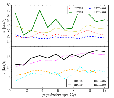
Figure 19: Velocity dispersions of stellar populations of different ages in the dwarf galaxy models, the upper and lower panel respectively show the LDT models and the HDT models. For all models the last snapshots were taken, their stellar populations divided into 12 equal age bins, and for each age bin the velocity dispersion was calculated in a box with width $R_{e}$ around the center of the galaxy.

7 Conclusion

In this paper we investigated how, in simulated dwarf galaxies in isolation, metallicity gradients are formed, how they evolve and how, once formed, they can be maintained. Furthermore, we adressed the importance of dynamical orbit-changing processes in the dwarf galaxy regime, and their potential in erasing or weakening existing population gradients. We hereby also investigated the role of the density threshold for star formation.

Firstly, in Section 5, we found that metallicity gradients are gradually built up during the evolution of non-rotating dwarf galaxy models by ever more centrally concentrated star formation adding to the overall gradient. On themselves, the formed gradients easily survive and their strength hardly declines over several Gyr, indicating that only external disturbances would be able to significantly weaken or erase population gradients in dwarf galaxies. The metallicity gradients produced by our dwarf galaxy models are found to agree well with observed metallicity gradients of dwarf galaxies in the Local Group, both in shapes and slopes.

Secondly, from Section 6 we conclude that the orbital displacements of the stars are quite limited in our models, of the order of only fractions of the half light radius over time-spans of 5 to 10 Gyr in both our rotating and non-rotating models. This is contrary to what is found in massive disc galaxies, where scattering of stars off the corotation resonance of large-scale spiral structure can cause significant radial migration. The absence of long-lived, major spiral structures in the simulated dwarf galaxies leaves only turbulent gas motions and scattering off dense gas clouds as scattering agents of stars, leading to an only mild dynamical heating of the stellar body that allows for the long-term survival of population gradients.

Finally, increasing the density threshold for star formation from $0.1$ to $100~{}\mathrm{amu/cm^{-3}}$, which - together with increased feedback efficiency and novel cooling curves below $10^{4}$ K - represents a much more realistic description of star forming regions, has profound influences on the mode of star formation in our models. It produces high density, cold, star forming clumps, shorter star formation timescales, and lower stellar masses. On the matter of population gradient evolution and orbital displacements it also has a clear influence, producing stronger dynamical heating of the stellar particles which is seen through larger orbital displacements and clear trends in the velocity dispersion over different stellar populations. In absolute terms, however, the effect of this dynamical heating remains very limited.

References

- Alard (2001) Alard C., 2001, A&A, 377, 389
- Battaglia et al. (2006) Battaglia G., et al., 2006, A&A, 459, 423
- Battaglia et al. (2011) Battaglia G., Tolstoy E., Helmi A., Irwin M., Parisi P., Hill V., Jablonka P., 2011, MNRAS, 411, 1013
- Battaglia et al. (2012) Battaglia G., Rejkuba M., Tolstoy E., Irwin M. J., Beccari G., 2012, MNRAS, 424, 1113
- Bekki & Shioya (1999) Bekki K., Shioya Y., 1999, ApJ, 513, 108
- Bernard et al. (2008) Bernard E. J., et al., 2008, ApJ, 678, L21
- Chilingarian (2009) Chilingarian I. V., 2009, MNRAS, 394, 1229
- Cloet-Osselaer et al. (2012) Cloet-Osselaer A., De Rijcke S., Schroyen J., Dury V., 2012, MNRAS, 2952
- Crnojević, Grebel, & Koch (2010) Crnojević D., Grebel E. K., Koch A., 2010, A&A, 516, A85
- De Rijcke et al. (in preparation) De Rijcke S., Schroyen J., Vandenbroucke B., Decroos J., Jachowicz N., Cloet-Osselaer A., Koleva M., in preparation
- Dejonghe & de Zeeuw (1988) Dejonghe H., de Zeeuw T., 1988, ApJ, 333, 90
- den Brok et al. (2011) den Brok M., et al., 2011, arXiv, arXiv:1103.1218
- Gentile et al. (2004) Gentile G., Salucci P., Klein U., Vergani D., Kalberla P., 2004, MNRAS, 351, 903
- Gibson et al. (2013) Gibson B. K., Pilkington K., Brook C. B., Stinson G. S., Bailin J., 2013, arXiv, arXiv:1304.3020
- Governato et al. (2010) Governato F., et al., 2010, Nature, 463, 203
- Harbeck et al. (2001) Harbeck D., et al., 2001, AJ, 122, 3092
- Hopkins et al. (2009) Hopkins P. F., Cox T. J., Dutta S. N., Hernquist L., Kormendy J., Lauer T. R., 2009, ApJS, 181, 135
- Katz, Weinberg & Hernquist (1996) Katz N., Weinberg D. H., Hernquist L., 1996, ApJS, 105, 19
- Kaufmann, Wheeler, & Bullock (2007) Kaufmann T., Wheeler C., Bullock J. S., 200, MNRAS, 382, 1187
- Kirby et al. (2011) Kirby E. N., Lanfranchi G. A., Simon J. D., Cohen J. G., Guhathakurta P., 2011, ApJ, 727, 78
- Kirby, Cohen, & Bellazzini (2012) Kirby E. N., Cohen J. G., Bellazzini M., 2012, ApJ, 751, 46
- Koleva et al. (2009) Koleva M., de Rijcke S., Prugniel P., Zeilinger W. W., Michielsen D., 2009, MNRAS, 396, 2133
- Koleva et al. (2011) Koleva M., Prugniel P., de Rijcke S., Zeilinger W. W., 2011, MNRAS, 417, 1643
- Koleva et al. (2013) Koleva M., Bouchard A., Prugniel P., De Rijcke S., Vauglin I., 2013, MNRAS, 428, 2949
- Lépine, Acharova, & Mishurov (2003) Lépine J. R. D., Acharova I. A., Mishurov Y. N., 2003, ApJ, 589, 210
- Lianou, Grebel, & Koch (2010) Lianou S., Grebel E. K., Koch A., 2010, A&A, 521, A43
- Loebman et al. (2011) Loebman S. R., Roškar R., Debattista V. P., Ivezić Ž., Quinn T. R., Wadsley J., 2011, ApJ, 737, 8
- Łokas, Kazantzidis, & Mayer (2011) Łokas E. L., Kazantzidis S., Mayer L., 2011, ApJ, 739, 46
- Łokas, Kowalczyk, & Kazantzidis (2012) Łokas E. L., Kowalczyk K., Kazantzidis S., 2012, arXiv, arXiv:1212.0682
- Maio et al. (2007) Maio U., Dolag K., Ciardi B., Tornatore L., 2007, MNRAS, 379, 963
- Mateo (1998) Mateo M. L., 1998, ARA&A, 36, 435
- McQuinn et al. (2010) McQuinn K. B. W., et al., 2010, ApJ, 724, 49
- Monelli et al. (2012) Monelli M., et al., 2012, MNRAS, 422, 89
- Navarro, Frenk & White (1996) Navarro J. F., Frenk C. S., White S. D. M., 1996, ApJ, 462, 563
- Pipino et al. (2010) Pipino A., D’Ercole A., Chiappini C., Matteucci F., 2010, MNRAS, 407, 1347
- Revaz et al. (2009) Revaz Y., Jablonka P., Sawala T., Hill V., Letarte B., Irwin M., Battaglia G., Helmi A., Shetrone M. D., Tolstoy E., Venn K. A., 2009, A&A, 501, 189
- Revaz & Jablonka (2012) Revaz Y., Jablonka P., 2012, A&A, 538, A82
- Roškar et al. (2008) Roškar R., Debattista V. P., Stinson G. S., Quinn T. R., Kaufmann T., Wadsley J., 2008, ApJ, 675, L65
- Roškar et al. (2012) Roškar R., Debattista V. P., Quinn T. R., Wadsley J., 2012, MNRAS, 426, 2089
- Roychowdhury et al. (2010) Roychowdhury S., Chengalur J. N., Begum A., Karachentsev I. D., 2010, MNRAS, 404, L60
- Sánchez-Janssen, Méndez-Abreu, & Aguerri (2010) Sánchez-Janssen R., Méndez-Abreu J., Aguerri J. A. L., 2010, MNRAS, 406, L65
- Sawala et al. (2010) Sawala T., Scannapieco C., Maio U., White S., 2010, MNRAS, 402, 1599
- Schönrich & Binney (2009) Schönrich R., Binney J., 2009, MNRAS, 399, 1145
- Schroyen et al. (2011) Schroyen J., De Rijcke S., Valcke S., Cloet-Osselaer A., Dejonghe H., 2011, MNRAS, 416, 601
- Sellwood & Binney (2002) Sellwood J. A., Binney J. J., 2002, MNRAS, 336, 785
- Shen, Wadsley, & Stinson (2010) Shen S., Wadsley J., Stinson G., 2010, MNRAS, 407, 1581
- Spergel et al. (2007) Spergel D. N., et al., 2007, ApJS, 170, 377
- Spitzer & Schwarzschild (1953) Spitzer L., Jr., Schwarzschild M., 1953, ApJ, 118, 106
- Springel (2005) Springel V., 2005, MNRAS, 364, 1105
- Springel et al. (2005) Springel V., et al., 2005, Natur, 435, 629
- Stinson et al. (2006) Stinson G., Seth A., Katz N., Wadsley J., Governato F., Quinn T., 2006, MNRAS, 373, 1074
- Stinson et al. (2007) Stinson G. S., Dalcanton J. J., Quinn T., Kaufmann T., Wadsley J., 2007, ApJ, 667, 170
- Stinson et al. (2009) Stinson G. S., Dalcanton J. J., Quinn T., Gogarten S. M., Kaufmann T., Wadsley J., 2009, MNRAS, 395, 1455
- Strigari et al. (2007) Strigari L. E., Koushiappas S. M., Bullock J. S., Kaplinghat M., 2007, PhRvD, 75, 083526
- Sutherland & Dopita (1993) Sutherland R. S., Dopita M. A., 1993, ApJS, 88, 253
- Tolstoy et al. (2004) Tolstoy E., et al., 2004, ApJ, 617, L119
- Valcke et al. (2008) Valcke S., De Rijcke S., Dejonghe H., 2008, MNRAS, 389, 1111
- Vandenbroucke et al. (in preparation) Vandenbroucke B., De Rijcke S., Schroyen J., Jachowicz N., in preparation
- Vazdekis et al. (1996) Vazdekis A., Casuso E., Peletier R. F., Beckman J. E., 1996, ApJS, 106, 307
- Walker et al. (2010) Walker M. G., Mateo M., Olszewski E. W., Peñarrubia J., Wyn Evans N., Gilmore G., 2010, ApJ, 710, 886
- Wechsler et al. (2002) Wechsler R. H., Bullock J. S., Primack J. R., Kravtsov A. V., Dekel A., 2002, ApJ, 568, 52