Crystal length effects on the angular spectrum of spontaneous parametric downconversion photon pairs

Abstract

We present a theoretical and experimental analysis of the joint effects of the transverse electric field distribution and of the nonlinear crystal characteristics on the properties of photon pairs generated by spontaneous parametric downconversion (SPDC). While it is known that for a sufficiently short crystal the pump electric field distribution fully determines the joint signal-idler properties, for longer crystals the nonlinear crystal properties also play an important role. In this paper we present experimental measurements of the angular spectrum (AS) and of the conditional angular spectrum (CAS) of photon pairs produced by spontaneous parametric downconversion (SPDC), carried out through spatially-resolved photon counting. In our experiment we control whether or not the source operates in the short-crystal regime through the degree of pump focusing, and explicitly show how the AS and CAS measurements differ in these two regimes. Our theory provides an understanding of the boundary between these two regimes and also predicts the corresponding differing behaviors.

I Introduction

The process of spontaneous parametric downconversion (SPDC) burnham70 has been used for the generation of paired photons in many recent experiments, ranging from fundamental tests of quantum mechanics zeilinger99 to implementations of quantum information processing protocols kok07 . In this process a laser pump beam illuminates a second-order non-linear crystal, where individual pump photons are annihilated giving rise to the emission of signal and idler photon pairs. In particular, these photon pairs exhibit a rich transverse spatial structure rubin96 ; joobeur94 , which forms the subject matter of the present study. Photon pairs entangled in the spatial degree of freedom, including the specific case of entanglement in orbital angular momentum mair01 ; molina-terriza07 , are of interest because each photon can be described by a multi-dimensional Hilbert space howell04 ; law04 ; walborn07 ; fedorov08 ; straupe11 ; dilorenzopires09 compared to the case of polarization which is limited to a dimension of $2$ kwiat95 .

Spatially-resolved single-photon detection in the transverse momentum domain yields the angular spectrum (AS) of the SPDC bi-photon field, which for type-I SPDC has a well-known annular shape. If a single photon is detected at a certain location in the AS with transverse momentum value $\tilde{\textbf{k}}^{\bot}$, the conjugate photon can be detected in coincidence around the location which fulfills transverse momentum conservation, i.e. with transverse momentum value $-\tilde{\textbf{k}}^{\bot}$. This forms the basis for a second measurement of interest, in which the idler photon is detected at a certain transverse momentum value and where spatially-resolved coincidence detection of the signal photon yields the conditional angular spectrum (CAS), which may be thought of as the shape of the heralded signal-mode photon torres05 . An idealized plane-wave pump in the process of SPDC leads to strict transverse momentum correlations, so that each individual idler-mode $k$-vector in the AS is correlated to a single signal-mode $k$-vector, yielding a delta-like CAS. In contrast, for a realistic experimental situation involving finite transverse dimensions of the pump beam, these transverse momentum correlations are no longer strict, i.e. each individual idler-mode $k$-vector is correlated with a spread of signal-mode $k$-vectors, so that the CAS acquires a certain width.

The properties of spatially-entangled SPDC photon pairs, including the AS and CAS, are determined on the one hand by the transverse electric field distribution of the pump, and on the other hand by the nonlinear crystal properties, including crystal dispersion, length and Poynting vector walk off. The manner in which the pump transverse spatial properties are mapped to those of the SPDC photon pairs has been studied in a number of papers monken98 ; walborn10 ; joobeur94 ; law04 ; warborn03 ; torres05 ; grayson94 . It is known that for a sufficiently short crystal, the spatially-resolved rate of signal-idler coincidences is fully determined by the pump transverse electric field distribution monken98 ; walborn10 ; molina05 ; saleh00 ; lorenzo09 ; neves04bis ; lee05 ; walborn07 ; jha10 . Within this limit, it thus becomes straightforward to engineer photon pairs to have a particular spatial character, as determined by the pump. This forms the basis for a large body of work, which seeks to exploit particular types of spatial correlations present in SPDC photon pairs. Indeed, the short-crystal approximation has been used in the context of the implementation of quantum information processing protocols, in experiments which exploit the orbital angular momentum of SPDC photon pairs molina03 ; arnaut01 ; walborn04 ; peeters07 ; ren05 ; kawase09 , in ghost imaging and diffraction experiments pittman96 ; santos03 ; abouraddy01 ; almeida06 ; costa10 ; walborn11 , as well as in a variety of other recent experiments fonseca99 ; fonseca99bis ; walborn05 ; monken98bis ; fonseca99ter ; shimizu03 ; vidal08 ; neves06 ; lee06 ; deng06 ; ether06 . However, for a sufficiently long crystal or for a sufficiently focused pump beam, the photon pair properties are no longer solely determined by the pump spatial distribution. The objective of this paper is to provide an understanding of the SPDC photon-pair properties in general, including situations for which the short-crystal approximation can and cannot be used, as well as of the boundary between these two regimes.

We have performed a detailed study of the CAS and of how the AS properties are derived from those of the CAS, paying special attention to crystal length effects. We show that the CAS is given by the product of two separate functions, one which is related to the pump AS, and another one which is related to the properties of the nonlinear crystal, including length, dispersion and Poynting vector walkoff. In our study of crystal length effects, we show that a critical length $L_{c}$ exists, which depends on the degree of pump focusing, so that for $L<L_{c}$, crystal length effects can be neglected, and the CAS is fully determined by the pump AS; we show that in this case the CAS is a displaced version of the pump AS. We also show that for $L>L_{c}$, the CAS is determined both by the pump AS and the crystal properties. In this latter case, we show that the CAS becomes elongated to a degree related to the crystal length and tilted according to the location of the fixed detector, leading to azimuthal distinguishability.

We have carried out experimental measurements of the AS and CAS, exhibiting excellent agreement with numerical simulations based on our SPDC theory, which is general enough to include essentially all experimental aspects of interest, i.e an arbitrary pump spatial distribution, spatial and spectral filtering of the SPDC photons, crystal dispersion, Poynting vector walkoff, and the spatial extent of detectors. In particular, we have performed a careful experimental/numerical exploration of the AS and of the CAS, where we vary the degree of pump focusing klyshko82 ; lee05 ; bennink06 ; dilorenzopires11 ; suzer08 ; grice11 ; vicent10 in order to explore and contrast the resulting behavior in the $L<L_{c}$ and $L>L_{c}$ regimes. Our theory presented here explains the azimuthal distinguishability evident in the CAS measurements of Ref. osorio07 , making it clear that this distinguishability is a crystal-length effect which appears only for sufficiently long crystals ($L>L_{c}$). This paper leads to a quantitative and qualitative understanding, not available in previous works, of how the spatial character of SPDC photon pairs is determined by nonlinear crystal properties in addition to the pump angular spectrum, which should be useful for the design of photon pair sources for specific applications.

II Theory

The quantum state which describes photon pairs produced by SPDC is given by $|\Psi\rangle=|\mbox{vac}\rangle+\eta|\Psi_{2}\rangle$, with

$$\left|\Psi_{2}\right\rangle =\int d\omega_{s}\int d^{2}\textbf{k}_{s}^{\bot}\int d\omega_{i}\int d^{2}\textbf{k}_{i}^{\bot}F(\omega_{s},\textbf{k}^{\bot}_{s},\omega_{i},\textbf{k}^{\bot}_{i})$$ (1)

$$\times\hat{a}^{\dagger}(\omega_{s},\textbf{k}^{\bot}_{s})\hat{a}^{\dagger}(\omega_{i},\textbf{k}^{\bot}_{i})\left|\mbox{vac}\right\rangle$$

where $\eta$ is a constant related to the conversion efficiency, $F(\omega_{s},\textbf{k}^{\bot}_{s},\omega_{i},\textbf{k}^{\bot}_{i})$ represents the joint amplitude, $\hat{a}^{\dagger}_{\mu}(\omega_{s},\textbf{k}^{\bot}_{\mu})$ (with $\mu=s,i$) is the creation operator associated with the signal and idler modes, expressed as a function of the transverse wavevector $\textbf{k}^{\bot}_{\mu}$ and frequency $\omega_{\mu}$, and where $|\mbox{vac}\rangle$ is the vacuum. Taking into account spectral filters $f_{\mu}(\omega)$ applied to the signal and idler modes ($\mu=s,i$), the joint amplitude is given by

$$F(\omega_{s},\textbf{k}^{\bot}_{s},\omega_{i},\textbf{k}^{\bot}_{i})=A_{s}\ell(\omega_{s})A_{i}\ell(\omega_{i})\,f_{s}(\omega_{s})f_{i}(\omega_{i})$$

$$\times\phi(\omega_{s},\textbf{k}^{\bot}_{s},\omega_{i},\textbf{k}^{\bot}_{i})\alpha(\omega_{s}+\omega_{i}).$$ (2)

In Eq. II, we have used the definitions $\ell(\omega)\equiv\sqrt{\hbar\,\omega/[2(2\pi)^{3}\epsilon_{0}\,n(\omega)^{2}]}$, where $\epsilon_{0}$ is the permittivity of free space and $n(\omega)$ is the index of refraction, and $A_{\mu}\equiv k_{\mu}^{\prime}k_{\mu}/k_{\mu z}$. $\phi(\omega_{s},\textbf{k}^{\bot}_{s},\omega_{i},\textbf{k}^{\bot}_{i})$ is the phasematching function and $\alpha(\omega)$ is the spectral amplitude of the pump. $k_{\mu z}$ represents the longitudinal components of the signal and idler $k$-vectors, given by $k_{\mu z}=(k_{\mu}^{2}-|\textbf{k}_{\mu}^{\bot}|^{2})^{1/2}$, with $k_{\mu}=n(\omega_{\mu})\omega_{\mu}/c$. Primed quantities denote frequencyt derivatives. Let us define the transverse vector sum $\textbf{k}_{+}^{\bot}=\textbf{k}^{\bot}_{s}+\textbf{k}^{\bot}_{i}$, in terms of which the phase matching function can be expressed as

$$\phi(\omega_{s},\textbf{k}^{\bot}_{s},\omega_{i},\textbf{k}^{\bot}_{i}) = S(\textbf{k}_{+}^{\bot})\mbox{sinc}\left(\frac{1}{2}L\Delta k(\omega_{s},\textbf{k}^{\bot}_{s},\omega_{i},\textbf{k}^{\bot}_{i})\right)$$ (3)

$$\times \mbox{exp}\left(i\frac{1}{2}L\Delta k(\omega_{s},\textbf{k}^{\bot}_{s},\omega_{i},\textbf{k}^{\bot}_{i})\right).$$

Here, the function $S(\textbf{k}^{\bot})$ represents the pump transverse wave vector amplitude distribution, evaluated in the transverse wavevector sum $\textbf{k}_{+}^{\bot}$, so that $|S(\textbf{k}^{\bot})|^{2}$ represents the pump AS. The phasemismatch $\Delta k(\omega_{s},\textbf{k}^{\bot}_{s},\omega_{i},\textbf{k}^{\bot}_{i})$ can be expressed in terms of the pump wavenumber $k_{p}$, the Poynting vector walkoff angle experienced by the pump, $\rho_{0}$, and the y-component of the $\textbf{k}_{+}^{\bot}$ vector as

$$\Delta k(\omega_{s},\textbf{k}^{\bot}_{s},\omega_{i},\textbf{k}^{\bot}_{i})=k_{p}-\frac{|\textbf{k}_{+}^{\bot}|^{2}}{2\,k_{p}}-k_{sz}-k_{iz}-k_{+y}^{\bot}\,\mbox{tan}\rho_{0}.$$ (4)

Note that here we have assumed without loss of generality that walkoff occurs on the plane $zy$. In this paper we are interested in studying the transverse spatial structure of the emitted photon pairs, specifically through spatially-resolved photon counting experiments. Standard Fourier optics techniques may be used in order to probe this structure in either the transverse position, or the transverse wavevector momentum domains. Specifically, a map of counts as a function of the signal- and idler-mode transverse wavevector may be obtained by a detection scheme with transverse spatial resolution on the Fourier plane located a distance of one focal length $f$ from a lens of focal length $f$, itself placed a distance $f$ from the SPDC crystal. If two detectors are placed on the Fourier plane so that they collect photons with transverse wavevectors $\textbf{k}^{\bot}_{s}$ and $\textbf{k}^{\bot}_{i}$ and frequencies $\omega_{s}$ and $\omega_{i}$, the rate of signal and idler coincidences is given by

$$R_{c}(\omega_{s},\textbf{k}^{\bot}_{s},\omega_{i},\textbf{k}_{i}^{\bot})$$

$$=\langle\Psi_{2}|a^{\dagger}(\omega_{s},\textbf{k}_{s}^{\bot})a^{\dagger}(\omega_{i},\textbf{k}_{i}^{\bot})a(\omega_{i},\textbf{k}_{i}^{\bot})a(\omega_{s},\textbf{k}_{s}^{\bot})|\Psi_{2}\rangle.$$ (5)

In a given experimental situation, this rate of detection should be integrated over the transverse wavevector and spectral acceptance of the detectors.

We will specialize our discussion to the case of a continuous-wave pump, for which the pump may be regarded as essentially monochromatic at frequency $\omega_{p}$, and $|\alpha(\omega)|^{2}$ may be replaced by $\delta(\omega-\omega_{p})$. Assuming detectors with ideal transverse wavevector resolution, and integrating over the spectral content of the photon pairs, it may be shown that the rate of coincidences can then be written as follows

$$R^{(0)}_{c}(\textbf{k}^{\bot}_{s},\textbf{k}_{i}^{\bot})=|S(\textbf{k}_{+}^{\bot})|^{2}\mathscr{L}(\textbf{k}^{\bot}_{s},\textbf{k}^{\bot}_{i}).$$ (6)

Thus, the rate of coincidences can be factored into two contributions. On the one hand, $|S(\textbf{k}_{+}^{\bot})|^{2}$ is related to transverse phasematching and is fully determined by the pump angular spectrum. On the other hand, $\mathscr{L}(\textbf{k}^{\bot}_{s},\textbf{k}^{\bot}_{i})$ is related to longitudinal phasematching and is determined by the crystal, including the effects of the crystal length, dispersion and Poynting vector walkoff. This function is given by

$$\mathscr{L}(\textbf{k}_{s}^{\bot},\textbf{k}_{i}^{\bot}) =\int\mbox{d}\omega_{i}\,\frac{k_{s}^{\prime}k_{s}}{k_{sz}}\frac{k_{i}^{\prime}k_{i}}{k_{iz}}|f(\omega_{p}-\omega_{i})|^{2}\,|f(\omega_{i})|^{2}$$ (7)

$$\times\mbox{sinc}^{2}\left[\frac{1}{2}\,L\,\Delta k(\omega_{p}-\omega_{i},\textbf{k}^{\bot}_{s},\omega_{i},\textbf{k}^{\bot}_{i})\right].$$

Note that while $k_{\mu}$ and $k^{\prime}_{\mu}$ (with $\mu=s,i$) are functions of the signal and idler frequencies, $\omega_{p}-\omega_{i}$ and $\omega_{i}$, $k_{\mu z}$ is a function of these frequencies and of the corresponding transverse wavevector components. Let us consider the limit in which the pump beam is in the form of a plane wave, with transverse wavevector $\textbf{k}^{\bot}_{p}=0$. In this case, the function $|S(\textbf{k}^{\bot}_{+})|^{2}$ becomes

$$|S(\textbf{k}^{\bot}_{+})|^{2}=\delta(\textbf{k}^{\bot}_{+})=\delta(\textbf{k}^{\bot}_{s}+\textbf{k}^{\bot}_{i})$$ (8)

This equation tells us that if a single idler photon is detected at $\textbf{k}^{\bot}_{i}=\textbf{k}^{\bot}_{i0}$, the conjugate photons may be found at $\textbf{k}^{\bot}_{s}=-\textbf{k}^{\bot}_{i0}$ so that transverse momentum is exactly conserved. Note, however, that the probability of observing photon pairs at two such conjugate points is limited by the function $\mathscr{L}(-\textbf{k}_{i0}^{\bot},\textbf{k}_{i0}^{\bot})$, i.e. by the existence of longitudinal phasematching at these two transverse wavevector values.

Let us now consider the more general case where the pump is given by a superposition of plane waves, i.e. for which the pump AS is no longer a delta function. In this case, if a single photon is detected at $\textbf{k}^{\bot}_{i}=\textbf{k}^{\bot}_{i0}$ on the transverse wavevector space, the conjugate photons may be found around $\textbf{k}^{\bot}_{s}=-\textbf{k}^{\bot}_{i0}$ with an uncertainty which grows with the width of the pump angular spectrum. We then refer to the function $R_{c}(\textbf{k}^{\bot}_{s},\textbf{k}^{\bot}_{i0})$, which determines this uncertainty, as the conditional angular spectrum (CAS) of the signal photon, conditioned on the detection of a single idler photon with transverse wavevector $\textbf{k}^{\bot}_{i0}$. The function $|S(\textbf{k}^{\bot}_{s}+\textbf{k}^{\bot}_{i0})|^{2}$, which for a sufficiently broad $\mathscr{L}(\textbf{k}_{s}^{\bot},\textbf{k}_{i0}^{\bot})$ represents the signal-photon CAS, is a displaced version of the pump AS, centered at $\textbf{k}^{\bot}_{s}=-\textbf{k}^{\bot}_{i0}$.

Specifically, let us consider the case where the pump beam is in the form of a Gaussian beam with widths $W_{x}$ and $W_{y}$ along the $x$ and $y$ directions. In this case, $|S(\textbf{k}^{\bot}_{+})|^{2}$ is given by

$$|S(\textbf{k}^{\bot}_{+})|^{2}=\exp\biggl{(}-\frac{1}{2}\{W_{x}^{2}\,(k_{+x}^{\bot})^{2}+W_{y}^{2}\,(k_{+y}^{\bot})^{2}\}\biggr{)},$$ (9)

in terms of the $x$ and $y$ components of the vector $\textbf{k}_{+}^{\bot}$. As the pump beam is increasingly focused, corresponding to smaller values of $W_{x}$ and $W_{y}$, the pump AS becomes broader also leading to a broader CAS, as limited by the function $\mathscr{L}(\textbf{k}_{s}^{\bot},\textbf{k}_{i}^{\bot})$. Thus, the strict one-to-one transverse momentum signal and idler correlations which appear in the plane-wave pump limit become weaker as the pump is increasingly focused.

So far we have considered idealized detection of the signal and idler modes involving a single transverse wavevector value. However, in a realistic experimental implementation, the transverse dimensions of the detectors used for the signal and idler modes are non-vanishing. Suppose that the transverse wavevector acceptance of each detector is characterized by functions $u_{s}(\textbf{k}^{\bot}-\textbf{k}^{\bot}_{s})$ and $u_{i}(\textbf{k}^{\bot}-\textbf{k}^{\bot}_{i})$ for the signal and idler modes respectively, where each of the detectors is centered at $\textbf{k}^{\bot}=\textbf{k}^{\bot}_{\mu}$ (with $\mu=s,i$). Then, the resulting coincidence rate obtained with these detectors can be written as

$$R_{c}(\textbf{k}^{\bot}_{s},\textbf{k}^{\bot}_{i}) = \int d^{2}\tilde{\textbf{k}}^{\bot}_{s}\int d^{2}\tilde{\textbf{k}}^{\bot}_{i}R^{(0)}_{c}(\tilde{\textbf{k}}^{\bot}_{s},\tilde{\textbf{k}}^{\bot}_{i})$$ (10)

$$\times u_{s}(\tilde{\textbf{k}}^{\bot}_{s}-\textbf{k}^{\bot}_{s})u_{i}(\tilde{\textbf{k}}^{\bot}_{i}-\textbf{k}^{\bot}_{i}).$$

Let us now turn our attention to single-channel counts, i.e. obtained through a single detector. The rate of single-channel counts obtained by a detector placed so that it selects single photons with transverse wavevector $\textbf{k}^{\bot}_{s}$ and frequency $\omega_{s}$, is given by

$$R_{s}(\omega_{s},\textbf{k}^{\bot}_{s})= \langle\Psi_{2}|a^{\dagger}(\omega_{s},\textbf{k}_{s}^{\bot})a(\omega_{s},\textbf{k}_{s}^{\bot})|\Psi_{2}\rangle$$ (11)

In a given experimental situation, this rate of detection should be integrated over the transverse wavevector and spectral acceptance of the detector. It may be shown that under the same conditions in which Eq. 6 was derived, the rate of single-channel detection is related to the CAS through the following simple relationship

$$R_{s}^{(0)}(\textbf{k}^{\bot}_{s})=\int d^{2}\tilde{\textbf{k}}^{\bot}_{i}R^{(0)}_{c}(\textbf{k}^{\bot}_{s},\tilde{\textbf{k}}_{i}^{\bot}).$$ (12)

The above quantity represents the transverse-wavevector distribution, or angular spectrum (AS), of the SPDC photon pairs. Thus, according to Eq. 6, the SPDC AS evaluated at a wavector $\textbf{k}^{\bot}_{s}=\textbf{k}^{\bot}_{s0}$ is given by the CAS $R^{(0)}_{c}(\textbf{k}^{\bot}_{s0},\textbf{k}_{i}^{\bot})$ integrated over all $\textbf{k}_{i}^{\bot}$ values.

When evaluating Eq. 12 for type-I non-collinear SPDC one obtains a well-known annular structure on the $\textbf{k}_{s}^{\bot}$ plane. In the next section, we will show experimental results, as well as simulations based on Eq. 12, which show this annular structure, and how it differs in the two regimes of interest, namely those for which the short-crystal approximation can and cannot be used.

In the case of a non-ideal detector characterized by an acceptance function $u_{s}(\textbf{k}^{\bot}-\textbf{k}^{\bot}_{s})$, the signal-mode angular spectrum may be written as

$$R_{s}(\textbf{k}^{\bot}_{s})=\int d^{2}\tilde{\textbf{k}}^{\bot}_{s}\int d^{2}\tilde{\textbf{k}}^{\bot}_{i}R^{(0)}_{c}(\tilde{\textbf{k}}^{\bot}_{s},\tilde{\textbf{k}}^{\bot}_{i})u(\tilde{\textbf{k}}^{\bot}_{s}-\textbf{k}^{\bot}_{s}).$$ (13)

For the discussion of the experimental results, below, it is useful to consider the single-channel and double-channel detection rates as a function of the transverse coordinates on the Fourier plane, behind an $f$-$f$ optical system, i.e. $R_{s}(\bm{\rho}_{s}^{\bot})$ and $R_{c}(\bm{\rho}_{s}^{\bot},\bm{\rho}_{i}^{\bot})$. If the signal and idler modes each involve a single emission frequency, then these functions are simply scaled versions of their counterparts in the wavevector domain, according to the transformation $\textbf{k}^{\bot}_{\mu}=[\omega/(c\,f)]\bm{\rho}^{\bot}_{\mu}$ (with $\mu=s,i$), where $f$ is the focal length used in the $f$-$f$ optical system, i.e. each transverse position on the Fourier plane corresponds to a specific transverse momentum value. However, because this transformation is frequency-dependent, if the emitted modes contain a spread of frequencies the rate of single-channel detection in the position and wavevector domains are not simply scaled versions of each other. When carrying out simulations, care must be taken to integrate the functions $R_{s}(\bm{\rho}_{s}^{\bot})$ and $R_{c}(\bm{\rho}_{s}^{\bot},\bm{\rho}_{i}^{\bot})$ over the detected spectral components.

In Fig. 1 we show the geometry of the SPDC emission annulus for non-collinear type-I SPDC from a negative uniaxial, specifically beta barium borate (BBO), crystal. We denote by $\vec{k}_{p}$ the wavevector corresponding to the central direction of propagation of the pump beam, by $\vec{S}$ the pump Poynting vector, and by $\vec{C}$ the crystal axis. Note that the angular separation between $\vec{S}$ and $\vec{k}_{p}$ is due to Poynting vector walkoff. We also show two pairs of signal and idler rays born at two distinct planes, projected on the $y$-$z$ and $x$-$z$ planes. As may be appreciated in the figure, because photon pairs are born along the path of $\vec{S}$, on the $y$-$z$ plane the two upper rays have a greater separation from $\vec{S}$ compared to the two lower rays, while the two corresponding separations are equal on the $x$-$z$ plane. This leads to an asymmetry in the emission annulus. Note that while for the above argument, we have implicitly assumed a transversely well-localized pump beam, the pump beam in fact has horizontal and vertical widths $W_{x}$ and $W_{y}$. If these widths are considerably larger that the lateral ray displacement $L\tan\rho_{0}$, the annulus asymmetry is in fact suppressed. In other words, this asymmetry is visible only for a sufficiently focused beam so that $W_{x},W_{y}\lesssim L\tan\rho_{0}$. Note that this asymmetry, mediated by pump focusing and Poynting vector walkoff, is the origin of so called “hot spots” which have been observed in the spatial flux distribution of type-II parametric downconversion koch95 .

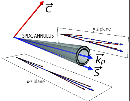
Figure 1: (color online) Schematic of emission annulus with various source characteristics indicated.

In Fig. 2 we show simulations of the AS for the case of a Gaussian beam pump, based on numerical integration of Eqns. 6 and 12. The AS is shown as a contour plot for two different degrees of focusing ($W_{x}=182.0\mu$m, $W_{y}=189.0\mu$m for panel a and $W_{x}=38.9\mu$m, $W_{y}=34.7\mu$m for panel b; note that these choices of beam widths correspond to experimental situations presented below). For these plots we have assumed a $1$mm long BBO crystal cut at $29.3^{\circ}$, for non collinear type-I phasematching. Note that while the annulus is symmetric, with a constant width, in the case of panel a, it becomes asymmetric with an azimuthally-varying width for panel b, as indeed is to be expected from the argument in the previous paragraph. This annulus asymmetry apparent in the single-channel counts spatial distribution also translates into azimuthal distinguishability of the photon pairs around the annulus (i.e. into an azimuthal variation of the orientation and width of the CAS) osorio07 . In order to illustrate this, in both panels of Fig. 2 we also show the CAS corresponding to $7$ points (shown as white dots) chosen to be angularly equidistant on the left-hand side of the angular spectrum. For three of these points (top, left and bottom) we show in addition plots of the $|S(\textbf{k}_{+}^{\bot})|^{2}$ and $\mathscr{L}(\textbf{k}^{\bot}_{s},\textbf{k}^{\bot}_{i})$ functions, the product of which yields the CAS. Note that the AS asymmetry may be explained in terms of clipping of the $|S(\textbf{k}_{+}^{\bot})|^{2}$ function by the $\mathscr{L}(\textbf{k}^{\bot}_{s},\textbf{k}^{\bot}_{i})$ function. For example, for a fixed detector at the top of the annulus, the corresponding CAS in a focused pump regime is narrowed by the horizontal structure of the $\mathscr{L}(\textbf{k}^{\bot}_{s},\textbf{k}^{\bot}_{i})$ function. Thus, the AS at the top of the annulus given as the integral over all $\textbf{k}^{\bot}_{i}$ values of the CAS will have a lower value compared, say, to the diametrically opposed portion of the annulus where this clipping does not occur. As will be discussed below, while panel $a$ corresponds to the short-crystal $L<L_{c}$ regime, panel $b$ corresponds to the $L>L_{c}$ regime.

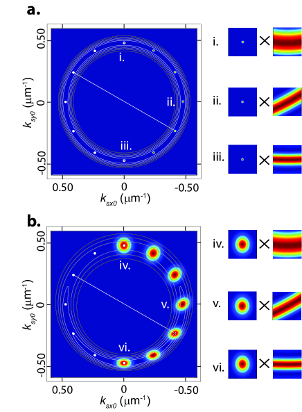
Figure 2: (color online) Contour plot of the angular spectrum for two different experimental situations (panel a: $W_{x}=182.0\mu$m, and $W_{y}=189.0\mu$m and panel b: $W_{x}=38.9\mu$m, and $W_{y}=34.7\mu$m), along with white dots covering one half of the annulus, angularly equi-spaced by $30^{\circ}$, along with the conditional angular spectrum corresponding to each of these white dots. For each of the two panels we also show, for the CAS corresponding to a fixed detector on the bottom, left and top of the AS, plots of the functions $|S(\textbf{k}^{\bot}_{s}+\textbf{k}^{\bot}_{i})|^{2}$ and $\mathscr{L}(\textbf{k}^{\bot}_{s},\textbf{k}^{\bot}_{i})$ the product of which yields the CAS.

It is interesting to relate the CAS in the spontaneous case which we study in this paper, to the size of speckles obtained in the spatial intensity distribution in the case of high-gain, i.e. stimulated parametric downconversion brambilla04 ; jedrkiewicz04 ; jedrkiewicz06 ; blanchet10 ; brida09 ; blanchet08 . Indeed, SPDC photons with a given transverse angular momentum $\textbf{k}^{\bot}$ within the AS can serve as a seed for parametric amplification, leading to the appearance of coupled speckles at $\textbf{k}^{\bot}$ and $-\textbf{k}^{\bot}$. According to the analysis in Refs. brambilla04 ; brida09 , the mean speckle area (also sometimes referred to as coherence area), is inversely proportional to the pump beam transverse area, an effect which mimics the observed dependence of the area in transverse momentum space of our CAS on the focusing strength.

Note on the one hand that the function $\mathscr{L}(\textbf{k}^{\bot}_{s},\textbf{k}^{\bot}_{i})$ depends only on crystal properties; in particular, its width is determined by the crystal length $L$ with longer crystals yielding narrower widths. Note on the other hand that the function $|S(\textbf{k}_{+}^{\bot})|^{2}$ depends only on pump properties, and its width corresponds to the pump angular width, i.e. it is determined by the degree of pump focusing. Thus, for a given degree of pump focusing there is a critical crystal length $L_{c}$ such that for $L<L_{c}$ the function $\mathscr{L}(\textbf{k}^{\bot}_{s},\textbf{k}^{\bot}_{i})$ is wider than the function $|S(\textbf{k}_{+}^{\bot})|^{2}$ so that the latter fully determines the CAS. In contrast, for $L>L_{c}$, the CAS is determined by both of these functions together, i.e. by crystal properties in addition to pump properties. Note from Fig. 2 that a plot of the function $\mathscr{L}(\textbf{k}^{\bot}_{s},\textbf{k}^{\bot}_{i})$ yields a stripe which is horizontally-oriented at the top and bottom of the annulus, with a larger width at the top, and which is oriented diagonally at other annulus locations, with a maximum tilt at the left and right. This azimuthal variability of the function $\mathscr{L}(\textbf{k}^{\bot}_{s},\textbf{k}^{\bot}_{i})$ is the origin of the azimuthal distinguishability of photon pairs. In particular, areas outside of the structure of function $\mathscr{L}(\textbf{k}_{s}^{\bot},\textbf{k}_{i}^{\bot})$, which may be diagonal, are “removed” from the plot of function $|S(\textbf{k}_{s}^{\bot}+\textbf{k}_{i}^{\bot})|^{2}$ and can yield a narrowed and tilted CAS.

It is thus interesting to consider the AS and CAS in the short-crystal regime ($L\ll L_{c}$). In this limit, the $\mathscr{L}(\textbf{k}_{s}^{\bot},\textbf{k}_{i}^{\bot})$ function is much broader than the $|S(\textbf{k}_{s}^{\bot}+\textbf{k}_{i}^{\bot})|^{2}$ function, so that the conditional angular spectrum is determined by the latter, according to

$$R^{(0)}_{c}(\textbf{k}^{\bot}_{s},\textbf{k}_{i}^{\bot})\approx|S(\textbf{k}_{+}^{\bot})|^{2}.$$ (14)

Note that because the CAS in Eq. 14 depends only on the pump AS, it is azimuthally invariant. It is also interesting to consider the amplitude underlying this conditional angular spectrum. In the case of ideal idler detection involving a single transverse wavevector $\tilde{\textbf{k}}^{\bot}_{i}$ and frequency $\tilde{\omega}_{i}$, and within the short crystal regime, the state describing the heralded signal-mode single photon may be written as follows

$$|\Psi\rangle_{s}=\kappa\int d\textbf{k}^{\bot}_{s}A_{s}S(\textbf{k}^{\bot}_{s}+\tilde{\textbf{k}}^{\bot}_{i})|\omega_{p}-\tilde{\omega}_{i},\textbf{k}^{\bot}_{s}\rangle.$$ (15)

where $\kappa$ is a normalization constant. It may be seen that under these conditions, the signal-mode single-photon wavevector amplitude constitutes a displaced version of the pump wavevector amplitude, centered at $-\tilde{\textbf{k}}_{i}$. Also, in the $L\ll L_{c}$ regime, $\mathscr{L}(\textbf{k}_{s}^{\bot},\textbf{k}_{i}^{\bot})$ is a slowly-varying function and may be considered a constant for the purposes of the integration in Eq. 12. Thus, the AS is given as follows, where we use the fact that the integral of the pump AS over all transverse wavevectors represents the pump power, i.e. a constant,

$$R^{(0)}_{s}(\textbf{k}^{\bot}_{s}) \propto \mathscr{L}(\textbf{k}^{\bot}_{s},-\textbf{k}^{\bot}_{s}).$$ (16)

Thus, in the short-crystal regime, while the CAS depends only on the transverse phasematching properties through the function $|S(\textbf{k}^{\bot}_{+})|^{2}$, the AS depends only on longitudinal phase matching properties through the function $\mathscr{L}(\textbf{k}^{\bot}_{s},-\textbf{k}^{\bot}_{s})$. In order to make the previous discussion more quantitative, let us define $\tilde{\textbf{k}}^{\bot}_{i}=(0,k^{\bot}_{iy})$ with $k^{\bot}_{iy}>0$ chosen so as to maximize the single-channel counts. Then, we can define the $1/e$ full widths of the functions $|S(\textbf{k}^{\bot}_{s}+\tilde{\textbf{k}}^{\bot}_{i})|^{2}$ and $\mathscr{L}(\textbf{k}^{\bot}_{s},\tilde{\textbf{k}}^{\bot}_{i})$, along the $k_{y}$ direction, as $\delta k_{S}$ and $\delta k_{\mathscr{L}}$, respectively. Fig. 3(a) shows a plot of $\delta k_{\mathscr{L}}$ as a function of the crystal length obtained numerically (continuous line) for a BBO crystal with a $29.3^{\circ}$ cut angle; note that longer crystals lead to a smaller width $\delta k_{\mathscr{L}}$. Fig. 3(a) also shows $\delta k_{S}$ for the case of a Gaussian beam pump, plotted with dashed lines for different values of $W=W_{x}=W_{y}$, (indicated, in microns, within the black rectangles). We then define the critical crystal length $L_{c}$, for a given pump beam radius $W$, as that for which $\delta k_{\mathscr{L}}=\delta k_{S}$.

Fig. 3(b) represents the parameter space $\{W,L\}$, where we have assumed $W_{x}=W_{y}=W$, and where we include a plot of the condition $L=L_{c}$, obtained numerically, which turns out to have an essentially linear dependence on $W$; note that this condition cannot easily be obtained analytically. This line divides the parameter space in two parameter sub-spaces; the right-hand sub-space represents the set of all experimental configurations in the regime $L<L_{c}$, while the left-hand subspace represents the set of all experimental configurations in the regime $L>L_{c}$. Also shown in the plot are four dots indicating our four experimental configurations (see discussion below; in particular dots 1 and 4 correspond to panels a and b of Fig. 2). Thus, on the one hand, in the limit of a plane wave pump, $L_{c}\rightarrow\infty$, and the CAS is fully determined by the pump properties without any influence of the crystal properties regardless of the crystal length. In this case, the CAS exhibits no variations around the SPDC annulus, and the photon pairs are thus azimuthally indistinguishable. On the other hand, a greater degree of focusing (corresponding to smaller values of $W$), leads to a smaller critical crystal length $L_{c}$. Thus, a sufficiently focused pump and/or a sufficiently long crystal implies that photon pairs are in the regime $L>L_{c}$, in which case the CAS becomes elongated and tilted leading to azimuthal distinguishability.

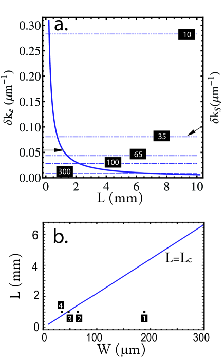
Figure 3: (color online) In panel a) we show the widths of the functions $\mathscr{L}(\textbf{k}^{\bot}_{s},\textbf{k}^{\bot}_{i})$ and $|S(\textbf{k}^{\bot}_{s}+\textbf{k}^{\bot}_{i})|^{2}$ as a function of the crystal length, for a fixed value of $\textbf{k}^{\bot}_{i}$ corresponding to the top of the AS, for different values of the pump beam radius indicated in microns within the black squares. In panel b) we show the condition $L=L_{c}$ plotted in the parameter space $\{W,L\}$ obtained from the intersections in panel a. We also indicate the four experimental measurements (see below) with labelled black dots.

Related results were obtained in Ref. burlakov97 . In this paper, it was found theoretically that for a sufficiently short crystal, and/or for sufficiently small emission angles, the transverse variation of the crystal nonlinearity - pump amplitude product determines the conditional angular spectrum, while the angular spectrum is in this case determined solely by the nonlinear crystal properties. Conversely, the paper by Burlalkov et al. reports that for a sufficiently long crystal, and/or for sufficiently large emission angles, the nonlinear crystal properties determine the conditional angular spectrum while the angular spectrum becomes sensitive to the transverse variation of the crystal nonlinearity - pump amplitude product.

III Experiment

The objective of our experimental work presented here is to characterize the angular distribution of the SPDC photon pairs, both in terms of single-channel and double-channel detection events where we use variations in the degree of pump focusing to select whether the source is in the $L<L_{c}$ or $L>L_{c}$ regime.

Our experimental setup is shown schematically in Fig. 4. A beam from a diode laser (DL) centered at $406.8$nm is used as pump for the SPDC process. This beam is spatially filtered by coupling into a single-mode fiber (not shown in the figure) and using the collimated out-coupled beam, with $23$mW power. A blue colored glass filter (Schott BG-39; not shown in the figure) is used in order to suppress non-ultraviolet background photons. The resulting beam illuminates a $1$mm-thick $\beta$-barium borate (BBO) crystal, cut at a phasematching angle of $29.3^{\circ}$ for type-I non-collinear phasematching so that the degenerate photon pairs produced propagate outside the crystal at an angle of $3.6^{\circ}$ with respect to the axis defined by the pump beam. Pump photons are suppressed by transmitting the signal and idler modes through a long-pass filter with a cut-on wavelength of $488$nm (F1), followed by a bandpass filter centered at $810$nm with a $10$nm bandwidth (F2); both of these filters are placed normal to the axis defined by the pump beam. A lens with a focal length of $10$cm (L2) is placed at a distance of $10$cm from the crystal, thus defining the Fourier plane a further $10$cm from the lens.

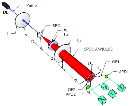
Figure 4: (color online) Experimental setup used for measuring the angular spectrum, and the conditional angular spectrum of SPDC photon pairs.

As discussed in the previous section, spatially-resolved photon counting may be implemented with the help of spatial filters placed on the Fourier plane, leading to single-photon detectors (APD1 and APD2). In our experiment, we have used for this purpose the fiber tips of large-diameter optical fibers (OF1 and OF2). Note that coupling of photon pairs into single-mode fibers is described through the mathematical overlap between the two-photon state and the fiber collection modes vicent10 . However, in the present case where fibers are highly multi-mode, the incoherent sum of the joint spectrum, projected onto all combinations of supported modes makes detection phase-insensitive. While in the case of the AS measurement a single fiber tip is used, in the case of the CAS measurement two separate fiber tips are used, one for each of the signal and idler modes. The fiber tips are mounted so that they can be displaced on the transverse plane, along the two perpendicular directions: $x$, parallel to the optical table, and $y$ normal to the optical table. In the AS case, the fiber tip displacement is carried out with computer-controlled linear motors ($50$nm resolution and $1.5$cm travel), and the fiber used has a $200\mu$m diameter core. In the CAS case, one of the fiber tips (corresponding to the idler mode) can be translated manually along the two axes, while the other fiber tip can be translated with our computer-controlled linear motors. Both of the fibers used have a $200\mu$m diameter core.

For the AS measurement, the fiber tip scans a sufficient transverse area in order to encompass the entire emission annulus. For the CAS measurement, a location $\textbf{k}^{\bot}_{i0}$ for the idler-mode fiber tip is selected on the SPDC annulus, which determines by transverse momentum conservation the expected location, $-\textbf{k}^{\bot}_{i0}$, for the conjugate signal photons. In our experiments we have chosen $\textbf{k}^{\bot}_{i0}$, with a vanishing $y$ component $k_{iy0}$, and with a negative value of $k_{ix0}$ (left side of the SPDC cone looking into the crystal) chosen so that the number of counts is maximized. The signal-mode fiber tip is then scanned over an area around $-\textbf{k}^{\bot}_{i0}$.

The optical fibers (a single one for the AS measurement, and two of them for the CAS measurement) lead to fiber-coupled silicon single-photon counting modules (SPCM’s). The electronic pulses generated by the SPCM’s are inverted, attenuated and discriminated to produce standard nuclear instrumentation module (NIM) pulses of 7ns duration. These signals are on the one hand directly counted with pulse counters (C1 and C2 in Fig. 4), to yield single-channel counts. On the other hand, these signals form the inputs for an AND gate (&) which produces an output pulse when the two inputs are temporally overlapped. The output from the AND gate is counted by a third pulse counter (C3), to obtain the coincidence counts. We have in the region of $200$ background counts per second, including dark counts, in each of our two detectors. This level of background counts leads to essentially no accidental coincidence counts related to dark counts.

We have carried out AS and CAS measurements for four different pump-beam focusing strengths. These situations correspond to: i) no focusing lens used, and to a focusing lens with the following focal lengths used: ii) $f_{1}=30$cm, iii) $f_{1}=10$cm, and iv) $f_{1}=6$cm. In all cases, the lens is placed a distance of one focal length from the crystal. Note that the resulting pump beamwaist is not necessarily precisely centered with respect to the crystal; while in our theory, the AS and CAS depend on the beam radii $W_{x}$ and $W_{y}$ at the beamwaist, these functions do not depend on the beamwaist location with respect to the crystal’s center plane vicent10 . The values of $W_{x}$ and $W_{y}$, directly measured by recording the beam profile with a CCD camera at a number of distinct propagation planes and fitting to the standard beam radius vs propagation distance expression for Gaussian beams, are shown in Table 1, along with the resulting critical length $L_{c}$. Note that since the crystal length used is $1$mm, measurements 1 and 2 are in the $L<L_{c}$ regime, while measurement 3 is essentially on the boundary and measurement 4 is in the $L>L_{c}$ regime. Note also that the choice of parameters for each of the four measurements is indicated in Fig. 3(b) by labelled dots, where the horizontal coordinate is determined by the corresponding $W_{y}$ value from Table  1; indeed, for a fixed detector at the top of the AS, the CAS depends largely on $W_{y}$. The values of $W_{x}$ and $W_{y}$ shown in the table were used for the numerical simulations of the AS and of the CAS to be presented below for each of the measurements (1 through 4).

Measurement	$W_{x}$ ($\mu$m)	$W_{y}$ ($\mu$m)	$L_{c}$ (mm)
1) no lens used	182.0	189.0	4.1
2) $f_{1}=30$cm	67.5	64.8	1.4
3) $f_{1}=10$cm	56.4	47.9	1.1
4) $f_{1}=6$cm	38.9	34.7	0.8

Table 1: Vertical ($W_{y}$) and horizontal ($W_{x}$) beam widths, at the beamwaist, measured for each of the four measurements.

For each of these four cases, we have carried out a measurement of the AS, and a corresponding numerical simulation. These results are shown in Figure 5, which is organized in four blocks, for each of the focusing strengths from Table 1. Panels (a)-(d) correspond to measurement $1$, panels (e)-(h) to measurement $2$, and so forth. Within each of these blocks, the first panel represents a measurement of the AS shown in six gray levels, as indicated by the gray level bar on the left. Note that background counts have been subtracted for each of the AS measurements. For these measurements, data was taken on a transverse position grid, involving a counting period of $1$ second at each point. Each grid point represents a particular transverse position $\bm{\rho}_{s0}^{\bot}$ of the fiber tip, which corresponds to a transverse momentum value $\textbf{k}_{s0}^{\bot}=[\omega_{s}/(cf_{2})]\bm{\rho}_{s0}^{\bot}$. A grid spacing of $200\mu$m is used for measurements $1-3$ and of $250\mu$m is used for measurement $4$ in AS measurements, while a larger spacing of $400\mu$m is used for measurements $1-3$ and of $500\mu$m for measurement $4$ in areas of low counts, e.g. inside the annuli. The second panel represents the corresponding numerical simulation, where we have scaled the maximum number of counts to coincide with the experimentally-obtained maximum number of counts. The specific simulation carried out yields $R_{s}(\bm{\rho}_{s0}^{\bot})$ by numerical integration of Eq. 12; for convenience, we have also labeled these plots with the transverse momentum values at the degenerate SPDC frequency. Note that because the transverse dimensions of the fiber used for photon collection is negligible compared with the width of the AS annulus, in computing our numerical simulations we have used the expression corresponding to delta-like detectors on the Fourier plane (Eq. 12 rather than Eq. 13).

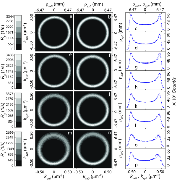
Figure 5: For measurement 1: (a) Experimentally-measured angular spectrum, with level of counts shown in gray-scale bar, (b) Corresponding numerical simulation, (c) The dots show the result of adding up the rows of the matrix of values in panel (a), the line shows the AS integrated over the $\rho_{sx0}$ coordinate, (d) The dots show the result of adding up the columns of the matrix of values in panel (a), the line shows the numerically-obtained angular spectrum integrated over the $\rho_{sy0}$ coordinate. Blocks of panels (e)-(h), (i)-(l), and (m)-(p) are similar to block (a)-(d) for each of measurements $2$,$3$ and $4$.

The third and fourth panels in each block show projected angular spectra obtained by adding together values along columns of this grid, to obtain the horizontal projected AS, and likewise obtained by adding together values along rows of this grid in order to obtain the vertical projected AS. We employ these projected angular spectra for a careful comparison between measurements and simulations; note that while we could also use for this purpose a “slice” obtained for fixed $\rho_{sx0}$ (or fixed $\rho_{sy0}$), the projected angular spectra lead to considerably more counts per grid location, and therefore to better statistics. The continuous lines represent the corresponding numerical simulations, where the AS has been integrated over the $\rho_{sy0}$ coordinate to obtain the horizontal projected AS, and over the $\rho_{sx0}$ coordinate to obtain the vertical projected AS. In general terms it may be seen that increasing the degree of pump focusing (or decreasing $W_{x}$ and $W_{y}$) leads to an increasingly asymmetrical AS, along the vertical direction, with a larger width at the top of the annulus than at its bottom; note that, in contrast, the widths at the left and right of the annulus are comparable. As discussed above, this AS asymmetry appears for parameter combinations in the regime $L>L_{c}$. This asymmetry, which is related to Poynting vector walkoff, is clear from the vertical projected AS which exhibits a wider and shorter right-hand peak compared to the left-hand peak. In contrast, the horizontal projected angular spectrum is symmetric, both peaks exhibiting identical heights and widths. Related results obtained with a CCD camera have been reported, for type-II SPDC, in Refs. lee05 ; bennink06 and using a LED pump in Ref. tamosauskas10 . Note that the agreement between the experimental measurements and the numerical simulations is excellent.

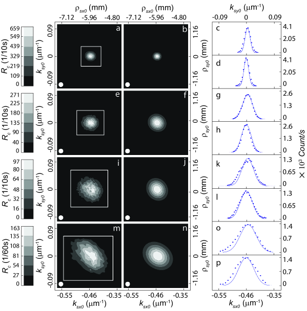
Figure 6: For measurement $1$: (a) Experimentally-measured conditional angular spectrum, with level of counts shown in gray-scale bar, (b) Corresponding numerical simulation, (c) The dots show the result of adding up the rows of the matrix of values in panel (a), the line shows the conditional angular spectrum integrated over the $\rho_{sx0}$ coordinate, (d) The dots show the result of adding up the columns of the matrix of values in panel (a), the line shows the numerically-obtained conditional angular spectrum integrated over the $\rho_{sy0}$ coordinate. Blocks of panels (e)-(h), (i)-(l), and (m)-(p) are similar to block (a)-(d) for each of measurements $2$,$3$ and $4$.

Let us now turn our attention to coincidence counts, i.e. to measurements of the conditional angular spectrum. As in the case of our measurements of the AS, we have undertaken measurements for the four experimental situations from Table 1. Likewise, for each of these four cases we have carried out a corresponding numerical simulation. These results are shown in Figure 6, which is organized in four blocks, for each of the focusing strengths from Table 1. Panels (a)-(d) correspond to measurement $1$, panels (e)-(h) to measurement $2$, and so forth. Within each of these blocks, the first panel represents a measurement of the conditional angular spectrum, shown in six gray levels, as indicated by the gray level bar on the left. For these measurements, data was taken on a transverse position grid, located around the transverse position conjugate to the position of the idler-mode fiber. Each grid point represents a particular transverse position $\bm{\rho}_{s0}^{\bot}$ of the fiber tip, which corresponds for SPDC frequency $\omega_{s}$ to a transverse momentum value $\textbf{k}_{s0}^{\bot}=[\omega_{s}/(cf_{2})]\bm{\rho}_{s0}^{\bot}$. We have used a counting period of $10$ seconds at each point for measurements $1-3$, and of $60$ seconds at each point for measurement $4$. These counting periods reflect the fact that for a greater degree of focusing, the counts become spread out over a greater transverse area, so that the level of counts at each grid point is reduced. A grid spacing of $50\mu$m is used for measurements $1-3$ and of $100\mu$m is used for measurement $4$. The white frame which encompasses the region with counts represents the range of transverse positions where data was taken; for positions outside of this frame, the coincidence counts were fixed to zero in the plots. We show the transverse dimensions of the fiber core used for photon collection through a white disk appearing near the bottom-left corner of each panel. It may be appreciated that the transverse extent of the collection fiber can be significant compared to the width of the measured CAS. In contrast, note that in the case of the AS (single-channel counts; Fig 5), the transverse dimensions of the fiber may be neglected, since they are much smaller than the width of the AS annulus. In fact, a white disk which represents the fiber core transverse dimensions is shown in Fig. 5, although it is difficult to see due to its small size.

The second panel in each block represents the corresponding numerical simulation, where we have scaled the maximum number of counts to coincide with the experimentally-obtained maximum number of counts. Note that for these simulations we have assumed that the spatial filter functions $u_{s}(\textbf{k}^{\bot}_{s}-\textbf{k}^{\bot}_{s0})$ and $u_{i}(\textbf{k}^{\bot}_{i}-\textbf{k}^{\bot}_{i0})$ are Gaussian with a full width at $1/e$ of $200\mu$m. The specific simulation carried out yields $R_{c}(\bm{\rho}_{s}^{\bot},\bm{\rho}_{i0}^{\bot})$ by numerical integration of a version of Eq. 10 written in terms of transverse position; for convenience, we have also labeled these plots with the transverse momentum values at the degenerate SPDC frequency. Note that because in the case of the CAS the transverse width of the fiber is significant, in computing our numerical simulations, we have used Eq. 10, which takes into account the transverse extent of detectors on the Fourier plane, rather than Eq. 6 which assumes delta-like detectors. Note also that in the case of coincidence counts, there are no background counts; the plots show the actual number of counts without subtracting a background level. The maximum number of coincidence counts decreases as the strength of focusing is increased so that the data is of greater quality for lower focusing strengths. The third and fourth panels in each block show projected conditional angular spectra obtained by adding together values along columns of this grid, to obtain the horizontal projected AS, and likewise obtained by adding together values along rows of this grid in order to obtain the vertical projected AS. As in the case of single-channel counts we employ these projected angular spectra for a careful comparison between measurements and simulations. The continuous lines represent the corresponding numerical simulations, where the angular spectrum has been integrated over the $\rho_{sy0}$ coordinate to obtain the horizontal projected AS, and over the $\rho_{sx0}$ coordinate to obtain the vertical projected AS. As can be appreciated, the agreement is excellent.

It is clear from our experimental and numerical results that an increased level of pump focusing broadens the CAS, and that for a sufficiently long crystal ($L>L_{c}$), the CAS may become tilted. Indeed, as expected from our theory, the CAS in fact corresponds to a displaced pump angular spectrum, which for $L>L_{c}$ may become clipped by function $\mathscr{L}(\textbf{k}^{\bot}_{s},\textbf{k}^{\bot}_{i})$ and can then become tilted. Thus, a greater degree of pump focusing leads to a broader pump angular spectrum, and this in turn leads to a broader CAS.

Note that for, both, the AS and CAS measurements, in the case of measurement $4$, i.e. the most highly focused case that we have considered, the agreement is not as optimal as for measurements $1-3$. We have observed that despite the use of spatial filtering through a single mode fiber, for an increasing degree of focusing, the pump beam acquires additional structure and becomes progressively less Gaussian. Since our theory assumes a perfectly Gaussian pump beam, this explains the observed slight discrepancy between theory and experiment for measurement 4.

IV Conclusions

We have presented a theoretical and experimental exploration of the joint effects of the pump transverse electric field distribution and of the non-linear crystal on the properties of photon pairs generated by spontaneous parametric downcinversion (SPDC). We have focused this analysis on the angular spectrum (AS) and on the conditional angular spectrum (CAS) of the SPDC photon pairs. We have shown that the CAS may be written as the product of two functions, one which is related to transverse phasematching and depends on pump properties, and another one which is related to longitudinal phasematching and depends on nonlinear crystal properties. We have shown that a critical crystal length $L_{c}$ exists, which depends on the degree of pump focusing, such that for $L<L_{c}$ the CAS is fully determined by the pump AS, and that for $L>L_{c}$ the CAS is determined jointly by crystal and pump properties. For a Gaussian beam pump, $L_{c}$ turns out to have an essentially linear relationship with the beam radius. Thus, the condition $L=L_{c}$ divides the $\{W,L\}$ parameter space into two separate parameter subspaces, where $L<L_{c}$ leads to a symmetric AS and to an azimuthally invariant CAS, and where $L>L_{c}$ leads to an asymmetric AS and to a CAS which varies in width and orientation around the SPDC annulus.

We have also presented experimental measurements of the AS and CAS for photon pairs generated through type-I non-collinear spontaneous parametric downconversion. These measurements were carried out by spatially-resolved photon counting, and by coincidence spatially-resolved photon counting, respectively. We have presented experimental data for the AS and CAS, along with corresponding numerical simulations based on our theory, for four different experimental configurations amongst which the degree of pump focusing is varied. A comparison of our experimental measurements with our numerical simulations leads to excellent agreement. Of the four experimental configurations used, two are in the regime $L<L_{c}$, one is near $L=L_{c}$, and one is in the regime $L>L_{c}$. Our measurements show that, as expected from our theory, pump focusing leads to an asymmetric broadening of the AS, and to a broadening and tilting of the CAS. Physically, the broadened AS is a consequence of the greater spread of pump transverse wavevectors, resulting in phasematching for a greater spread of signal and idler transverse wavevectors. This results in broadening of the conditional angular spectrum, so that each idler-mode $k$-vector is correlated to a spread of signal-mode $k$-vectors, while this correlation is one-to-one in the idealized case of a plane-wave pump. We believe that these results will lead to an enhanced quantitative and qualitative understanding of the spatial properties of type-I, non-collinear spontaneous parametric downconversion photon pairs and to an important tool for source design.

- (1) Burnham D C and Weinberg W L 1970 Phys. Rev. Lett. 25 84.
- (2) See for example Zeilinger A 1999 Rev. Mod. Phys. 71 S288.
- (3) See for example Kok P, Munro W J, Nemoto J K, Ralph T C, Dowling J P and Milburn G J 2007 Rev. Mod. Phys. 79 135.
- (4) Rubin M H 1996 Phys. Rev. A 54 5349–5360
- (5) Joobeur A, Saleh B E A, and Teich M C 1994 Phys. Rev. A 50 3349.
- (6) Mair A, Vaziri A, Weihs G and Zeilinger A 2001 Nature 412 313.
- (7) Molina-Terriza G, Torres J P and Torner L 2007 Nature Physics 3 305.
- (8) Howell J C, Bennink R S, Bentley S J and Boyd R W 2004 Phys. Rev. Lett. 92 210403.
- (9) Law C K and Eberly J H 2004 Phys. Rev. Lett. 92 127903.
- (10) Walborn S P and Monken C H 2007 Phys. Rev. A 76 062305
- (11) Fedorov M V, Efremov M A, Volkov P A, Moreva E V, Straupe S S and Kulik S P 2008 Phys. Rev. A 77 032336.
- (12) Straupe S S, Ivanov D P, Kalinkin A A, Bobrov I B and Kulik S P 2011 Phys. Rev. A 83 060302.
- (13) Di Lorenzo Pires H, Monken C H and van Exter M P 2009 Phys. Rev. A 80 022307.
- (14) See for example Kwiat P G, Mattle K, Weinfurter H, Zeilinger A, Sergienko A V and Shih Y 1995 Phys. Rev. Lett. 75, 4337.
- (15) Molina-Terriza G, Minardi S, Deyanova Y, Osorio C I, Hendrych M and Torres J P 2005 Phys. Rev. A 72 065802.
- (16) Torres J P, Molina-Terriza G and Torner L 2005 J. Opt. B: Quantum Semiclass. Opt. 7, 235.
- (17) Monken C H, Souto Ribeiro P H and Pádua S 1998 Phys. Rev. A 57 3123.
- (18) Walborn S P, Monken C H, Pádua S and Souto Ribero P H 2010 Phys. Rep. 495 87.
- (19) Walborn S P, de Oliveira A N, Pádua S and Monken C H 2003 Phys. Rev. Lett. 90, 143601.
- (20) Grayson T P and Barbosa G A 1994, Phys. Rev. A 49, 2948.
- (21) Saleh B E A, Abouraddy A F, Sergienko A V and Teich M C 2000 Phys. Rev. A 62, 043816.
- (22) Di Lorenzo Pires H and van Exter M P 2009 Phys. Rev. A 79 041801.
- (23) Neves L, Pádua S and Saavedra C 2004 Phys. Rev. A 69 042305.
- (24) Jha A K and Boyd R W 2010 Phys. Rev. A 81 013828.
- (25) Fonseca E J S, Monken C H, Pádua S and Barbosa G A 1999 Phys. Rev. A 59 1608.
- (26) Fonseca E J S, Souto Ribeiro P H, Pádua S and Monken C H 1999 Phys. Rev. A 60 1530.
- (27) Walborn S P, Nogueira W A T, de Oliveira A N, Pádua S and Monken C H 2005 Mod. Phys. Lett. B 19, 1
- (28) Monken C H, Souto Ribeiro P H and Pádua S 1998 Phys. Rev. A 57, R2267.
- (29) Fonseca E J S, Monken C H and Pádua S 1999 Phys. Rev. Lett. 82, 2868.
- (30) Shimizu R, Edamatsu K and Itoh T 2003 Phys. Rev A 67 041805(R)
- (31) Vidal I , Cavalcanti S B, Fonseca E J S and Hickmann J M 2008 Phys. Rev. A 78 033829.
- (32) Neves L, Lima G, Aguirre-Gomez J G, Monken C H, Saavedra C and P ádua S 2006 Mod. Phys. Lett. B 20 1.
- (33) Lee P S K and van Exter M P 2006 Phys. Rev. A 73 063827.
- (34) Deng L P, Dang G F and Wang K 2006 Phys. Rev. A 74 063819.
- (35) Molina-Terriza G, Torres J P and Torner L 2003 Opt. Commun. 228 155.
- (36) Arnaut H H and Barbosa G A 2001 Phys. Rev. Lett. 85, 286.
- (37) Walborn S P, de Oliveira A N, Thebaldi R S and Monken C H 2004 Phys. Rev. A 69 023811.
- (38) Peeters W H, Verstegen E J K and van Exter M P 2007 Phys. Rev. A, 76 042302.
- (39) Ren X F, Guo G P, Li J, and Guo G C 2005 Phys. Lett. A 341 81.
- (40) Kawase D, Miyamoto Y, Takeda M, Sasaki K, and Takeuchi S 2009 J. Opt. Soc. Am. B 26, 797.
- (41) Pittman T B, Strekalov D V, Klyshko D N, Rubin M H, A.V. Sergienko, and Y.H. Shih, Phys. Rev. A 53, 2804. (1996).
- (42) Santos I F, Sagioro M A, Monken C H and Padua S 20003 Phys. Rev. A 67 033812.
- (43) Abouraddy A F, Nasr M B, Saleh B E A, Sergienko A V and Teich M C 2001 Phys. Rev. A 63 063803.
- (44) Almeida M P, Huguenin J A O, Souto Ribeiro P H and Khoury A Z 2006 J. Mod. Opt. 53 777.
- (45) da Costa Moura A G, Nogueira W A T and Monken C H 2010 Opt. Commun. 283 2866.
- (46) Walborn S P, Ribeiro P H S and Monken C H 2011 Opt. Express 19, 17308.
- (47) Ether D S, Souto Ribeiro P H, Monken C H, and de Matos Filho R L 2006 Phys. Rev. A 73 053819.
- (48) Klyshko D N, Zh. Eksp. Teor. Fiz. 1982 83 1313 [Sov. Phys. JETP 1982 56 753].
- (49) Lee P S K, van Exter M P and Woerdman W P 2005 Phys. Rev. A 72 033803.
- (50) Bennink R S, Liu Y, Earl D D and Grice W P 2006 Phys. Rev. A 74 023802.
- (51) Di Lorenzo Pires H, Coppens F M G J and van Exter M P 2011 Phys. Rev. A 83 033837.
- (52) Süzer O, Goodson III T G 2008 Opt. Express 16, 20166.
- (53) Grice W P, Bennink R S, Goodman D S, Ryan A T 2011 Phys. Rev. A 83 023810.
- (54) Vicent L E, U’Ren A B, Rangarajan R, Osorio C I, Torres J P, Zhang L and Walmsley I A 2010 New J. Phys. 12 093027
- (55) Osorio C I, Molina-Terriza G, Font B G, and Torres J P 2007 Opt. Express 15 14636.
- (56) Koch K, Cheung E C, Moore G T, Chakmakjian S H and Liu J M 1995 IEEE J. Quantum Electron. 31 769.
- (57) Brambilla E, Gatti A, Bache M and Lugiato L A 2004 Phys. Rev. A 69 023802.
- (58) Jedrkiewicz O, Jiang Y K, E. Brambilla, A Gatti, M. Bache, L. A. Lugiato and P. Di Trapani 2004 Phys. Rev. Lett. 93 243601.
- (59) Jedrkiewicz O, Brambilla E, Bache M, Gatti A, Lugiato L A, and Di Trapani P 2006 J. Mod. Opt. 53, 575.
- (60) Blanchet J L, Devaux F, Furfaro L and Lantz E 2010 Phys. Rev. A 81 043825.
- (61) Brida G, Meda A, Genovese M, Predazzi E and Ruo-Berchera I 2009 J. Mod. Opt. 56 201.
- (62) Burlakov AV, Chekhova MV, Klyshko DN, Kuilk SP, Penin AN, Shih YH, and Strekaolv DV 1997 Phys. Rev. A 56 3214.
- (63) Blanchet J L, Devaux F, Furfaro L and Lantz E 2008 Phys. Rev. Lett. 101 233604.
- (64) Tamošauskas G, Galinis J, Dubietis A and Piskarskas A 2010 Opt. Express 18 4310.