Interacting partially directed self avoiding walk. From phase transition to the geometry of the collapsed phase.

Abstract.

In this paper, we investigate a model for a $1+1$ dimensional self-interacting and partially directed self-avoiding walk, usually referred to by the acronym IPDSAW. The interaction intensity and the free energy of the system are denoted by $\beta$ and $f$, respectively. The IPDSAW is known to undergo a collapse transition at $\beta_{c}$. We provide the precise asymptotic of the free energy close to criticality, that is we show that $f(\beta_{c}-\varepsilon)\sim\gamma\varepsilon^{3/2}$ where $\gamma$ is computed explicitly and interpreted in terms of an associated continuous model. We also establish some path properties of the random walk inside the collapsed phase $(\beta>\beta_{c})$. We prove that the geometric conformation adopted by the polymer is made of a succession of long vertical stretches that attract each other to form a unique macroscopic bead and we establish the convergence of the region occupied by the path properly rescaled towards a deterministic Wulff shape.

1. Introduction

1.1. Model and physical insight

A solvent is said to be ”poor” for a given homopolymer if the chemical affinity between the solvent and the monomers constituting the homopolymer is low. When dipped in such a solvent, the homopolymer folds itself up to exclude the solvent and therefore adopts a collapsed conformation, that looks like a compact ball. If the quality of the solvent improves, the chemical affinity raises until it reaches a threshold above which the polymer extends itself in such a way that a positive fraction of its monomers are in contact with the solvent.

The interacting partially directed self-avoiding walk (IPDSAW) was introduced in [ZL68] as a partially directed model of an homopolymer in a poor solvent. The spatial configurations of the polymer of length $L$ ($L$ monomers) are modeled by the trajectories of a self-avoiding random walk on $\mathbb{Z}^{2}$ that only takes unitary steps upwards, downwards and to the right. Thus, the set of allowed $L$-step paths is

$$\mathcal{W}_{L}=\{w=(w_{i})_{i=0}^{L}\in(\mathbb{N}_{0}\times\mathbb{Z})^{L+1}:\, w_{0}=0,\,w_{L}-w_{L-1}=\rightarrow,$$

$$w_{i+1}-w_{i}\in\{\uparrow,\downarrow,\rightarrow\}\;\,\forall 0\leq i<L-1,$$

$$w_{i}\neq w_{j}\;\,\forall i<j\}.$$

Note that the choice of $w$ ending with an horizontal step is made for convenience only. We consider two different a priori laws on $\mathcal{W}_{L}$, uniform and non-uniform.

(1) The uniform model: all $L$-step paths have the same probability, i.e.,

$$\mathbf{P}_{L}(w)=\frac{1}{|\mathcal{W}_{L}|},\quad w\in\mathcal{W}_{L}.$$ (1.1)

(2) The non-uniform model: the $L$-step paths have the following law

• At the origin or after an horizontal step: the walker must step north, south or east with equal probability $1/3$.

• After a vertical step north (respectively south): the walker must step north (respectively south) or east with probability $1/2$.

Henceforth, we will focus on the uniform model since all our results can be adapted straightforwardly to the non-uniform model modulo a shift in the critical point $\beta_{c}$ and in the value of the constant $a_{\beta}$ defined before the Shape Theorem.

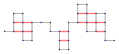
Figure 1. Example of a trajectory with 12 self-touchings in light grey.

The monomer-solvent interactions are not taken into account directly in the IPDSAW. We rather consider that, when dipped in a poor solvent, the monomers try to exclude the solvent and therefore attract one another. For this reason, any non-consecutive vertices of the walk though adjacent on the lattice are called self-touchings (see Fig. 1) and the interactions between monomers are taken into account by assigning an energetic reward $\beta\geq 0$ to the polymer for each self-touching (consequently, a lower chemical affinity corresponds to a larger $\beta$). Thus, we associate with every random walk trajectory $w=(w_{i})_{i=0}^{L}\in\mathcal{W}_{L}$ the Hamiltonian

$$H_{L}(w):=\sum_{\begin{subarray}{c}i,j=0\\ i<j-1\end{subarray}}^{L}\mathbf{1}_{\{\lVert w_{i}-w_{j}\rVert=1\}},$$ (1.2)

which allows to define the law $P_{L,\beta}$ of the polymer in size $L$ as,

$$P_{L,\beta}(w)=\frac{e^{\beta H_{L,\beta}(w)}}{Z_{L,\beta}}\mathbf{P}_{L}(w),$$ (1.3)

where $Z_{L,\beta}$ is the normalizing constant known as the partition function of the system. Henceforth, we remove the term $1/|{\mathcal{W}}_{L}|$ from the definition of $\mathbf{P}_{L}$ (recall (1.1)) and from the computation of the partition function $Z_{L,\beta}$. Although $\mathbf{P}_{L}$ is not a probability law anymore, the latter simplification is harmless, because it does not change the polymer law $P_{L,\beta}$ and because it only induces a constant shift of the free energy $f(\beta)$ introduced in Section 1.2 below.

From random walk paths to vertical stretches

It is easy to see that any path in ${\mathcal{W}}_{L}$ can be decomposed into a collection of vertical stretches separated by one horizontal step. Thus, we set $\Omega_{L}:=\bigcup_{N=1}^{L}\mathcal{L}_{N,L}$, where $\mathcal{L}_{N,L}$ is the set of all possible configurations consisting of $N$ vertical stretches that have a total length $L$, that is

$$\textstyle\mathcal{L}_{N,L}=\Bigl{\{}l\in\mathbb{Z}^{N}:\sum_{n=1}^{N}|l_{n}|+N=L\Bigr{\}}.$$ (1.4)

We build the natural one to one correspondence between $\Omega_{L}$ and ${\mathcal{W}}_{L}$ by associating with a given $l\in\Omega_{L}$ the path of ${\mathcal{W}}_{L}$ that starts at $0$, takes $|l_{1}|$ vertical steps north if $l_{1}>0$ and south if $l_{1}<0$, then takes one horizontal step, then takes $|l_{2}|$ vertical steps north if $l_{2}>0$ and south if $l_{2}<0$ then takes one horizontal step and so on… (see Fig. 2). The Hamiltonian associated with a given path of ${\mathcal{W}}_{L}$ can be rewritten in terms of its associated collection of vertical stretches $l\in\Omega_{L}$ as

$$\textstyle H_{L}(l_{1},\ldots,l_{N})=\sum_{n=1}^{N-1}(l_{n}\;\widetilde{\wedge}\;l_{n+1})$$ (1.5)

where

$$x\;\widetilde{\wedge}\;y=\begin{dcases*}|x|\wedge|y|&if $xy<0$,\\ 0&otherwise.\end{dcases*}$$ (1.6)

Therefore, the partition function can be rewritten under the form

$$Z_{L,\beta}=\sum_{N=1}^{L}\sum_{l\in\mathcal{L}_{N,L}}\ e^{\beta\sum_{i=1}^{N-1}(l_{i}\;\widetilde{\wedge}\;l_{i+1})}.$$ (1.7)

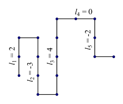
Figure 2. Example of a trajectory with $N=5$ vertical stretches and length $L=16$.

1.2. Free energy and collapse transition

The sequence $\{\log Z_{L,\beta}\}_{L}$ is super-additive and the Hamiltonian in (1.2) is obviously bounded from above by $\beta L$. As a consequence, we can define the free energy per step $f:(0,\infty)\to\mathbb{R}$ as

$$f(\beta)=\lim_{L\to\infty}\frac{1}{L}\log Z_{L,\beta}=\sup_{L\in\mathbb{N}}\frac{1}{L}\log Z_{L,\beta}\leq\beta.$$ (1.8)

The collapse transition corresponds to a loss of analyticity of $\beta\mapsto f(\beta)$ at some critical parameter $\beta_{c}\in(0,\infty)$ above which the density of self-touchings performed by the polymer equals $1$. In this collapsed phase, the expression of the free energy per step is rather simple, i.e., $\beta+\kappa$, where $\kappa$ is the entropic constant associated to those trajectories in ${\mathcal{W}}_{L}$ whose self-touching density is equal to $1+o(1)$. To achieve such a saturation of its self-touching, the polymer must choose its configuration among those satisfying two major geometric restrictions, i.e.,

• the number of horizontal steps is $o(L)$

• most pairs of consecutive vertical stretches are of opposite directions.

It turns out that an appropriate choice of a trajectory satisfying both restrictions above is sufficient to exhibit the collapsed free energy. To that aim, we pick $L\in\mathbb{N}\colon\sqrt{L}\in\mathbb{N}$ and consider the trajectory $l^{*}\in{\mathcal{L}}_{\sqrt{L},L}$ defined as $l^{*}_{i}=(-1)^{i-1}(\sqrt{L}-1)$ for $i\in\{1,\dots,\sqrt{L}\}$. By computing the contribution of $l^{*}$ to $Z_{L,\beta}$ one immediately obtain that, for $\beta>0$,

$$f(\beta)\geq\beta.$$ (1.9)

At this stage, we can define the excess free energy $\widetilde{f}(\beta):=f(\beta)-\beta$, which is always non negative by (1.9). We define the critical parameter

$$\beta_{c}:=\inf\{\beta\geq 0:\widetilde{f}(\beta)=0\},$$ (1.10)

and the convexity of $\beta\mapsto\widetilde{f}(\beta)$ allows us to partition $[0,\infty)$ into a collapsed phase denoted by $\mathcal{C}$ and an extended phase denoted by $\mathcal{E}$, i.e,

$$\mathcal{C}:=\{\beta:\widetilde{f}(\beta)=0\}=\{\beta:\beta\geq\beta_{c}\}$$ (1.11)

and

$$\mathcal{E}:=\{\beta:\widetilde{f}(\beta)>0\}=\{\beta:\beta<\beta_{c}\}.$$ (1.12)

1.3. Main results

The main results of this paper are Theorems A,B,C,D,E and F. Theorems A and B are dedicated to the investigation of the phase transition while the path properties of the polymer inside its collapsed phase are studied with Theorems C,D,E and F.

Before stating the Theorems we need to introduce $\mathbf{P}_{\beta}$ the law of an auxiliary symmetric random walk $V:=(V_{n})_{n\in\mathbb{N}}$ with geometric increments, i.e., $V_{0}=0$, $V_{n}=\sum_{i=1}^{n}U_{i}$ for $n\in\mathbb{N}$ and $(U_{i})_{i\in\mathbb{N}}$ is an i.i.d sequence under the law $\mathbf{P}_{\beta}$, with distribution

$$\mathbf{P}_{\beta}(U_{1}=k)=\tfrac{e^{-\frac{\beta}{2}|k|}}{c_{\beta}}\quad\forall k\in\mathbb{Z}\quad\text{with}\quad c_{\beta}:=\tfrac{1+e^{-\beta/2}}{1-e^{-\beta/2}}.$$ (1.13)

Then, for $\delta\geq 0$ we set

$$\mathfrak{h}_{\beta}(\delta):=\lim_{N\to\infty}\frac{1}{N}\log\mathbf{E}_{\beta}\bigl{(}e^{-\delta A_{N}(V)}\bigr{)},$$ (1.14)

where $A_{N}(V):=\sum_{i=1}^{N}|V_{i}|$ gives the geometric area below the $V$ trajectory after $N$ steps. We will prove in Section 2.2 below that the limit in (1.14) exists and that $\delta\mapsto\mathfrak{h}_{\beta}(\delta)$ is non-positive, non-increasing and continuous on $[0,\infty)$. We finally define $\Gamma(\beta)$ an energetic term of crucial importance as

$$\Gamma(\beta)=\tfrac{c_{\beta}}{e^{\beta}},$$ (1.15)

and we will see for instance in (1.36) below that $\Gamma(\beta)$ penalizes the horizontal steps when it is smaller than $1$ and favors them when it is larger than $1$.

A sharper asymptotic of the free energy close to criticality

With Theorem A, we give a new expression of the excess free energy.

Theorem A (Free energy equation).

The excess free energy $\widetilde{f}(\beta)$ is the unique solution of the equation $\log(\Gamma(\beta))-\delta+\mathfrak{h}_{\beta}(\delta)=0$ if such a solution exists and $\widetilde{f}(\beta)=0$ otherwise.

Note that Theorem A and the obvious equality $\mathfrak{h}_{\beta}(0)=0$ are sufficient to check that the critical parameter $\beta_{c}$ is the unique solution of $\Gamma(\beta)=1$. One of the main interest of Theorem A is that it allows us to use the analytic properties of $\delta\mapsto\mathfrak{h}_{\beta}(\delta)$ at $0^{+}$ to investigate the regularity of $\beta\mapsto\widetilde{f}(\beta)$ at $\beta_{c}$.

Theorem B (Phase transition asymptotics).

The phase transition is second order with critical exponent $3/2$ and the first order assymptotic of the excess free energy at $(\beta_{c})^{-}$ is given by

$$\lim_{\varepsilon\to 0^{+}}\frac{\widetilde{f}(\beta_{c}-\varepsilon)}{\varepsilon^{3/2}}=\Big{(}\frac{\varsigma_{1}}{\varsigma_{2}}\Big{)}^{3/2},$$ (1.16)

where

$$\varsigma_{1}=1+\tfrac{e^{-\beta_{c}/2}}{1-e^{-\beta_{c}}},$$ (1.17)

and where

$$\varsigma_{2}=-\lim_{T\to\infty}\frac{1}{T}\log\mathbf{E}\bigr{(}e^{-\sigma_{\beta_{c}}\int_{0}^{T}|B(t)|dt}\bigr{)}=2^{-1/3}|a^{\prime}_{1}|\sigma_{\beta_{c}}^{2/3},$$ (1.18)

with $\sigma_{\beta}^{2}=\mathbf{E}_{\beta}(U_{1}^{2})$, with $a^{\prime}_{1}$ the smallest zero (in absolute value) of the first derivative of the Airy function and with $(B_{s})_{s\in[0,\infty)}$ a standard Brownian motion.

Remark 1.1.

The Laplace transform $\mathbf{E}(e^{-s\int_{0}^{1}|B_{s}|ds})$ for $s>0$ was first computed analytically by Kac in [K46] and studied by Takacs [TA93] (see for instance the survey by Janson [J07]).

Remark 1.2.

The critical exponent $3/2$ is given by the leading term of the Taylor expansion of $\mathfrak{h}_{\beta}$ at $0^{+}$, i.e., $\mathfrak{h}_{\beta}(\gamma)\sim-c\,\gamma^{2/3}$ (with $c>0$). The method of proof we used consists in cutting the trajectories into blocs of size $\gamma^{-2/3}$. This very method was used in [HDHK03], in dimension $d=1$, to prove that discrete Domb-Joyce type models converge towards continuous Edwards type models in the weak coupling limit.

Remark 1.3.

The asymptotic $\mathfrak{h}_{\beta}(\gamma)\sim-c\,\gamma^{2/3}$ is closely related to the investigation of the so called pre-wetting phenomenon (see [HV04], where the scaling exponent is obtained from a renormalization procedure similar to ours). The pre-wetting phenomenon is observed when a thermodynamically stable gas is in contact with a substrate (hard-wall) that has a strong preference for the liquid phase. In such a situation, a thin layer of liquid may appear that separates the substrate from the gas. When the temperature $T$ gets closer to the liquid/gas boiling temperature $T_{b}$, the layer of liquid becomes thicker. The liquid-gas interface can therefore be modeled by a random walk trajectory constrained to remain positive and whose area is penalized via a Gibbs factor $\delta A_{N}(V)$ where $\delta$ vanishes as $T\to T_{b}$. Close to criticality ($\delta=0$), the correlation length of the system varies as $\delta^{-2/3}$ which explains the $2/3$ exponent of $\mathfrak{h}_{\beta}$ at $0^{+}$.

The determination of the precise asymptotics of the free energy close to $\beta_{c}$ brings the IPDSAW into a thin class of statistical mechanical models for which the behavior of the free energy close to criticality is well understood. This is the case, for instance for the pinning/wetting model (see [GIA11, Chapter 2]). Perturbing such models by adding a weak random component to their interactions is physically relevant (see [DHV92]) and gives rise to complex mathematical issues (see [AS06]). For the model of a polymer pinned by a linear interface, the issue of the disorder relevance on the phase transition was controversial until it was settled recently (see [DGLT09] or [GIA11, Chapters 4 and 5], for a survey). For the IPDSAW, a natural way of introducing the disorder would be to assign an energetic price $\beta+s\xi_{i,j}$ to the self-touching between monomers $i$ and $j$. The mechanism governing the phase transition being quite different from its counterpart in the pinning model, the investigation of the disorder effect is relevant both mathematically and physically.

Path properties inside the collapsed phase

The main result of this paper is concerned with the path behavior of the polymer inside its collapsed phase $(\beta>\beta_{c})$. We divide each trajectory into a succession of beads. Each bead is made of vertical stretches of strictly positive length and arranged in such a way that two consecutive stretches have opposite directions (north and south) and are separated by one horizontal step (see Fig. 3). A bead ends when the polymer gives the same direction to two consecutive vertical stretches or when a zero length stretch appears, which corresponds to two consecutive horizontal steps. We will prove that the polymer folds itself up into a unique macroscopic bead and we will identify its horizontal extension and its asymptotic deterministic shape. To quantify these results we need the following notations.

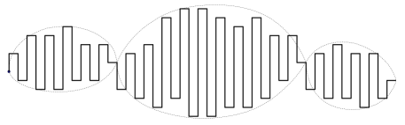
Figure 3. Example of a trajectory with $3$ beads.

Number of beads

Let $l\in\Omega_{L}$ and denote by $N_{L}(l)$ its horizontal extension, i.e., $N_{L}(l)$ is the integer $N$ such that $l\in{\mathcal{L}}_{N,L}$. Pick $l\in{\mathcal{L}}_{N,L}$ and let $(u_{j})_{j=1}^{N}$ be the sequence of accumulated lengths of the polymer after each vertical stretch, adding the lengths of the one step horizontal steps, that is $u_{j}=|l_{1}|+\dots+|l_{j}|+j$ for $j\in\{1,\dots,N\}$. For convenience only, set $l_{N+1}=0$. Set also $x_{0}=0$ and for $j\in\mathbb{N}$ such that $x_{j-1}<N$, set $x_{j}=\inf\{i\geq x_{j-1}+1\colon\,l_{i}\;\widetilde{\wedge}\;l_{i+1}=0\}$ (see Fig. 5). Finally, let $n_{L}(l)$ be the index of the last $x_{j}$ that is well defined, i.e., $x_{n_{L}(l)}=N$. Thus we can decompose any trajectory $l\in\Omega_{L}$ into a succession of $n_{L}(l)$ beads, each of them being associated with a subinterval of $\{1,\dots,L\}$ written as

$$I_{j}=\{u_{x_{j-1}}+1,\dots,u_{x_{j}}\},\quad\text{for}\quad j\in\{1,\dots,n_{L}(l)\},$$ (1.19)

and therefore, we can partition $\{1,\dots,L\}$ into $\cup_{j=1}^{n_{L}(l)}I_{j}$. At this stage, we can define the largest bead of a trajectory $l\in\Omega_{L}$ as $I_{j_{\text{max}}}$ with

$$j_{\text{max}}=\operatorname{arg\,max}\big{\{}|I_{j}|,j\in\{1,\dots,n_{L}(l)\}\big{\}}.$$ (1.20)

With Theorem C below, we claim that, in the collapsed phase, there is only one macroscopic bead.

Theorem C (One bead Theorem).

For $\beta>\beta_{c}$, there exists a $c>0$ such that

$$\lim_{L\to\infty}P_{L,\beta}\big{(}|I_{j_{\text{max}}}|\geq L-c\,(\log L)^{4}\big{)}=1.$$ (1.21)

Remark 1.4.

Dividing trajectories into beads does not give rise to an underlying renewal process as for instance, for the homogeneous pinning model when the trajectory is divided into excursions away from the origin (see for instance [cf:Gia, Chapter 2]). The fact that, after a bead of length $1$ the first stretch of the following bead can be either positive or negative whereas its orientation is constrained when the former bead is strictly larger than $1$ creates a dependency between consecutive beads that prevents us from rewriting the partition function with the help of an associated renewal process. However, if we omit the dependency between consecutive beads then, thanks to Proposition 4.2, the ”bead process” $(u_{x_{j}})_{j=0}^{n_{L}(l)}$ under $P_{L,\beta}$ can be related to a sub-exponential defective renewal process $\tau=(\tau_{i})_{i\geq 0}$ conditioned on $L\in\tau$. This latter process is characterized by an inter-arrival law $K:\overline{\mathbb{N}}\to[0,1]$ that satisfies $K(\infty)>0$ and $K(n)=k(n)e^{-c\sqrt{n}}$ with $k:\mathbb{N}\to\mathbb{N}$ a slowly varying function. Once conditioned by $\{L\in\tau\}$, it can be proven (see [cf:Gia, Appendix A.5] for the heavy tailed case or more recently [NT14] where the sub-exponential case is explicitly treated) that the number of renewals is $O(1)$ and that again there is only one macroscopic renewal (see e.g. [Asmussen03] for a general background on renewal theory).

Shape Theorem

First, recall the one-to-one correspondence between $\Omega_{L}$ and ${\mathcal{W}}_{L}$ described in Section 1.1 and denote by $w_{l}$ the path in ${\mathcal{W}}_{L}$ associated with a given family of vertical stretches $l\in\Omega_{L}$. Then, identify each $l\in\Omega_{L}$ with a connected compact subset of $\mathbb{R}^{2}$ denoted by $S_{L}(l)$ that extends the sites of $\mathbb{Z}^{2}$ occupied by $w_{l}$ to squares of length $1$, i.e.,

$$S_{L}(l)=\Big{\{}\cup_{i=0}^{L}w_{l}(i)+[-\tfrac{1}{2},\tfrac{1}{2}]^{2}\Big{\}},\quad l\in\Omega_{L}.$$ (1.22)

With Theorem D below we prove that, once rescaled horizontally and vertically by $\sqrt{L}$ the subset $S_{L}(l)$ converges in probability and for the Hausdorff distance towards ${\mathcal{S}}_{\beta}$ a deterministic subset of $\mathbb{R}^{2}$. Before defining ${\mathcal{S}}_{\beta}$ we need to settle some notation.

First, we denote by $\mathfrak{L}(h),h\in(-\tfrac{\beta}{2},\tfrac{\beta}{2})$ the logarithmic moment generating function of the random variable $U_{1}$, i.e,

$$\mathfrak{L}(h):=\log\mathbf{E}_{\beta}[e^{hU_{1}}],$$ (1.23)

and we introduce $\mathfrak{L}_{\Lambda}$

$${\textstyle\mathfrak{L}_{\Lambda}({\bf h}):=\int_{0}^{1}\mathfrak{L}(xh_{0}+h_{1})dx,}$$ (1.24)

which is defined on

$${\textstyle\mathcal{D}:=\Bigl{\{}{\bf h}=(h_{0},h_{1})\in\mathbb{R}^{2}\colon h_{1}\in\bigl{(}-\tfrac{\beta}{2},\tfrac{\beta}{2}\bigr{)},\ h_{0}+h_{1}\in\bigl{(}-\tfrac{\beta}{2},\tfrac{\beta}{2}\bigr{)}\Bigr{\}}.}$$ (1.25)

Then, we let $\widetilde{{\bf h}}(q,0):=(\widetilde{h}_{0}(q,0),\widetilde{h}_{1}(q,0))$ be the unique solution of the equation

$$\nabla\mathfrak{L}_{\Lambda}({\bf h})=(q,0)\,.$$ (1.26)

Since for $\beta>\beta_{c}$ the function

$$\widetilde{G}(a):=a\log\Gamma(\beta)-\tfrac{1}{a}\,\widetilde{h}_{0}\bigl{(}\tfrac{1}{a^{2}},0\bigr{)}+a\mathfrak{L}_{\Lambda}\bigl{(}\widetilde{\bf h}\bigl{(}\tfrac{1}{a^{2}},0\bigr{)}\bigr{)},$$ (1.27)

defined on $(0,\infty)$ is $C^{\infty}$, strictly concave and negative (see Section 4.4), we let $a_{\beta}>0$ be its unique maximizer.

We let $\gamma^{*}_{\beta}$ be the Wulff shape minimizing the rate function of Mogulskii large deviation principle (see [DZ, Theorem 5.1.2] ) applied to the random walk of law $\boldsymbol{\mathrm{P}}_{\beta}$, on the set containing the cadlag functions $\gamma:[0,1]\to\mathbb{R}$ satisfying $\gamma(1)=0$ and $\int_{0}^{1}\gamma(t)dt=1/a_{\beta}^{2}$ and endowed with the supremum norm $||\cdot||_{\infty}$. The following explicit formula holds (see Section 4.5):

$$\gamma^{*}_{\beta}(s)=\int_{0}^{s}\mathfrak{L}^{\prime}\big{[}(\tfrac{1}{2}-x)\,\widetilde{h}_{0}\big{(}\tfrac{1}{a_{\beta}^{2}},0\big{)}\big{]}dx,\quad s\in[0,1]\,.$$ (1.28)

Eventually we define the limiting shape

$${\mathcal{S}}_{\beta}=\big{\{}(x,y)\in\mathbb{R}^{2}\colon\,x\in[0,a_{\beta}],y\in\big{[}-\tfrac{1}{2}\,a_{\beta}\,\gamma^{*}_{\beta}(x/a_{\beta}),\tfrac{1}{2}\,a_{\beta}\,\gamma^{*}_{\beta}(x/a_{\beta})\big{]}\big{\}}$$ (1.29)

and we denote by $d_{H}$ the Hausdorff distance between subsets of $\mathbb{R}^{2}$.

Theorem D (Shape Theorem).

For $\beta>\beta_{c}$, we have convergence in $P_{L,\beta}$ probability for the Hausdorff distance towards a deterministic shape

$$\lim_{L\to\infty}P_{L,\beta}\Big{(}d_{H}\Big{(}\tfrac{S_{L}(l)}{\sqrt{L}},{\mathcal{S}}_{\beta}\Big{)}>\varepsilon\Big{)}=0\quad(\forall\varepsilon>0).$$ (1.30)

This shape Theorem is equivalent to the combination of Theorem E and Theorem F below. We display in Appendix A a proof of this equivalence.

Theorem E (Horizontal extension).

For $\beta>\beta_{c}$, for all $\varepsilon>0$

$$\lim_{L\to\infty}P_{L,\beta}\biggl{(}\Bigl{|}\frac{N_{L}(l)}{\sqrt{L}}-a_{\beta}\Bigr{|}>\varepsilon\biggr{)}=0.$$ (1.31)

Remark 1.5.

Determining the horizontal extension is challenging in the extended regime $(\beta<\beta_{c})$ and in the critical regime ($\beta=\beta_{c})$ as well. In the extended regime, we can already derive from the variational formula of the free energy in [NGP13, Theorem 1.2] that there exists $c_{2}>c_{1}>0$ so that $\lim_{L\to\infty}P_{L,\beta}(N_{L}(l)/L\in[c_{1},c_{2}])=1$. The extension is therefore of order $L$ and we expect that a law of large numbers also holds so that $N_{L}(l)/L$ converges in $P_{L,\beta}$ probability towards some constant $e_{\beta}\in(0,1)$. The critical regime is more delicate. In view of the random walk representation and since $\Gamma(\beta_{c})=1$, the law of $N_{L}(l)$ when $l$ is sampled from $P_{L,\beta}$ is exactly that of the stopping time $\tau_{L}:=\inf\{n\geq 1\colon n+A_{n}(V)\geq L\}$ of a random walk $V$ of law $\boldsymbol{\mathrm{P}}_{\beta}$ conditioned on $\{V_{\tau_{L}}=0,A_{\tau_{L}}=L-\tau_{L}\}$. We expect that a Donsker type invariance principle will hold there so that typically $A_{\tau_{L}}\sim\tau_{L}^{3/2}$ and thus we expect $N_{L}(l)/L^{2/3}$ to be tight under $P_{L,\beta}$.

The next Theorem gives the scaling limit of the upper and lower envelopes of the path in the collapsed phase. Pick $l\in{\mathcal{L}}_{N,L}$ and let ${\mathcal{E}}_{l}^{+}=({\mathcal{E}}^{+}_{l,i})_{i=0}^{N+1}$ be the path that links the top of each stretch consecutively (see Figure 4), while ${\mathcal{E}}_{l}^{-}=({\mathcal{E}}^{-}_{l,i})_{i=0}^{N+1}$ is the counterpart of ${\mathcal{E}}_{l}^{+}$ that links the bottom of each stretch consecutively. Thus, ${\mathcal{E}}^{+}_{l,0}={\mathcal{E}}^{-}_{l,0}=0$,

$${\mathcal{E}}^{+}_{l,i} =\max\{l_{1}+\dots+l_{i-1},l_{1}+\dots+l_{i}\},\quad i\in\{1,\dots,N\},$$ (1.32)

$${\mathcal{E}}^{-}_{l,i} =\min\{l_{1}+\dots+l_{i-1},l_{1}+\dots+l_{i}\},\quad i\in\{1,\dots,N\},$$ (1.33)

and ${\mathcal{E}}^{+}_{l,N+1}={\mathcal{E}}^{-}_{l,N+1}=l_{1}+\dots+l_{N}$. Then, let $\widetilde{\mathcal{E}}_{l}^{+}$ and $\widetilde{\mathcal{E}}_{l}^{-}$ be the time-space rescaled cadlag processes associated with ${\mathcal{E}}_{l}^{+}$ and ${\mathcal{E}}_{l}^{-}$ and defined as

$$\widetilde{\mathcal{E}}_{l}^{+}(t)=\frac{1}{N+1}\,{\mathcal{E}}^{+}_{l,{\lfloor t\,(N+1)\rfloor}}\quad\text{and}\quad\widetilde{\mathcal{E}}_{l}^{-}(t)=\frac{1}{N+1}\,{\mathcal{E}}^{-}_{l,{\lfloor t\,(N+1)\rfloor}},\quad t\in[0,1].$$ (1.34)

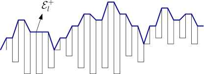
Figure 4. Example of the upper envelope of a trajectory

Theorem F (Wulff shape).

For $\beta>\beta_{c}$ and $\varepsilon>0$,

$$\lim_{L\to\infty}P_{L,\beta}\Big{(}\big{\|}\widetilde{\mathcal{E}}^{+}_{l}-\frac{\gamma^{*}_{\beta}}{2}\big{\|}_{\infty}>\varepsilon\Big{)} =0,$$

$$\lim_{L\to\infty}P_{L,\beta}\Big{(}\big{\|}\widetilde{\mathcal{E}}^{-}_{l}+\frac{\gamma^{*}_{\beta}}{2}\big{\|}_{\infty}>\varepsilon\Big{)} =0.$$ (1.35)

Note that $\widetilde{\mathcal{E}}^{+}_{l}-\widetilde{\mathcal{E}}^{-}_{l}$ (respectively, $(\widetilde{\mathcal{E}}^{+}_{l}+\widetilde{\mathcal{E}}^{-}_{l})/2$) is the rescaled version of the process that associates with each index $i\in\{1,\dots,N_{L}(l)\}$ the length $|l_{i}|$ of the $i$-th stretch (respectively, the height of the middle of the $i$-th stretch $l_{1}+\dots+l_{i-1}+\frac{l_{i}}{2}$). In view of Theorem F, the Wulff shape $\gamma^{*}_{\beta}$ happens to be the limit, as $L\to\infty$, of $\widetilde{\mathcal{E}}^{+}_{l}-\widetilde{\mathcal{E}}^{-}_{l}$. Such Wulff shape was identified, for instance in [DH96], as the limit of a random walk trajectory conditioned by fixing a large algebraic area between the path and the $x$-axis. However, the latter convergence is not sufficient to prove (F). We must indeed show that $(\widetilde{\mathcal{E}}^{+}_{l}+\widetilde{\mathcal{E}}^{-}_{l})/2$ converges to $0$ in probability.

Remark 1.6.

The Wulff shape construction, initially displayed in [W1901] appears in many models of statistical mechanics to describe the limiting shape of properly rescaled interfaces separating pure phases. Their construction is achieved by minimizing the integral of the surface tension along the continuous contours that satisfy some particular geometric constraint. A famous example arises from 2D Ising model in the phase transition regime. When considering a large square box of size $N$ with $-$ boundary condition and $T<T_{c}$, and by conditioning the total magnetization to be shifted from its mean ($-m^{*}N^{2}$) by a factor $a_{N}\gg N^{4/3}$, it was proven in [DKS92] at low temperature and then in [I94], [I95] and [IS98] up to $T_{c}$ that this magnetization shift is due to a unique $+$ island whose boundary, once rescaled by $1/\sqrt{a_{N}}$, converges towards a Wulff shape.

1.4. Relationship to earlier work

The IPDSAW and its continuous versions have attracted a lot of attention from physicists until very recently (see for instance [BDL09] or [HST13]). The main method that has been employed to investigate the IPDSAW involves combinatorial techniques (see [BGW92], [OPB93] or more recently [OP07]). To be more specific, this method consists in providing an analytic expression of the generating function $G(z)=\sum_{L=1}^{\infty}Z_{L,\beta}z^{L}$ whose radius of convergence $R$ satisfies $f=-\log R$. For a detailed version of the computations, we refer to [CHP12, p. 371–375].

The computation of the generating function $G$ allows us to determine the exact value of $\beta_{c}$ and to predict the behavior of the free energy close to criticality. However, the analytic expression of $G$ is very complicated and only gives an indirect access to the free energy. Furthermore, this combinatorial method does not allow to study an observable which does not grow like $L$, for instance, inside the collapsed phase, the horizontal extension is of order $\sqrt{L}$ and this can not be proven by such method.

A new approach has been developed in [NGP13] to work with the partition function directly. With the help of an algebraic manipulation of the Hamiltonian, that will be described in Section 2.1, it is indeed possible to rewrite the partition function in (1.7) under the form

$$Z_{L,\beta}=c_{\beta}\,e^{\beta L}\sum_{N=1}^{L}\left(\Gamma(\beta)\right)^{N}\mathbf{P}_{\beta}(\mathcal{V}_{N+1,L-N}),$$ (1.36)

where we recall (1.13) and (1.15) and where $\mathcal{V}_{n,k}$ is the set of those $n$-step trajectories of the random walk $V$ whose geometric area $A_{n}=\textstyle\sum_{i=1}^{n}|V_{i}|$ equals $k$, i.e.,

$$\mathcal{V}_{n,k}:=\big{\{}(V_{i})_{i=0}^{n}:\,A_{n}=k,\,V_{n}=0\big{\}}.$$ (1.37)

Thus, the excess free energy $\widetilde{f}(\beta)$ is the exponential growth rate of the summation in (1.36). In this new expression of the partition function, the term indexed by $N\in\{1,\dots,L\}$ in the summation corresponds to the contribution to the partition function of those trajectories $l\in{\mathcal{L}}_{N,L}$ (making $N$ horizontal steps).

This new approach was used in [NGP13, Theorem 1.2], to derive a variational expression of the excess free energy, which allowed us to prove that the collapsed transition is second order with critical exponent $3/2$.

Theorem 1.7 ([NGP13], Theorem 1.4).

The phase transition is of order $3/2$. That is, there exist two constants $c_{1},c_{2}>0$ such that for $\varepsilon$ small enough

$$c_{1}\,\varepsilon^{3/2}\leq\widetilde{f}(\beta_{c}-\varepsilon)\leq c_{2}\,\varepsilon^{3/2}.$$ (1.38)

With the present paper, we take the analysis of the phase transition two steps further (see Theorem B). In the first step, we establish the precise asymptotic: $\widetilde{f}(\beta_{c}-\varepsilon)\sim\gamma\varepsilon^{3/2}$ as $\varepsilon\searrow 0$ with $\gamma$ an explicit constant. In the second step, we give an expression of $\gamma$ in terms of the free energy of an auxiliary continuous model, that is $\mathsf{F}_{c}=\lim_{T\to\infty}\frac{1}{T}\log\mathbf{E}[\exp(-\int_{0}^{T}|B(t)|dt)]$. Moreover, the Laplace transform of $\int_{0}^{T}|B(t)|dt$ was computed by Kac in [K46] and this allows us to express $\mathsf{F}_{c}$ with the smallest zero (in modulus) of the derivative of the Airy function.

The question of the geometric conformation adopted by the polymer inside the collapsed phase has been raised and discussed by physicists in several papers, as for instance [POBG93]. It was believed that the monomers arrange themselves in a succession of long vertical stretches of opposite directions that constitute large beads. In this paper, we prove with Theorem C, that the polymer makes only one macroscopic bead and that the number of monomers (located at the beginning and at the end of the polymer) which do not belong to this bead grows at most like $(\log L)^{4}$. We also make rigorous the conjecture concerning the horizontal extension of the polymer, since we identify the limit in probability of $N_{L}/\sqrt{L}$, which turns out to be the constant extracted from an optimization procedure. We also establish the convergence of properly rescaled lower and upper envelopes to a deterministic Wulff shape. In particular, the typical vertical displacement of the middle point, the $L/2$-th monomer in a chain of length $L$, is of order $\sqrt{L}$.

There are numerical evidences that the vertical displacement of the endpoint grows as $L^{1/4}$ (see [POBG93], table II page 2394). This turns out to be a consequence of the typical behavior of the fluctuations of the envelopes around the Wulff shape, and this is not the topic of the present paper.

Finally, let us stress the fact that the convergence, in the collapsed phase, to a deterministic Wulff shape (see Theorem E) comes from a fairly complex procedure that needs to establish three properties:

1. The horizontal extension $N_{L}$ is of order $\sqrt{L}$.

2. There is only one macroscopic bead

3. When conditioned to be abnormally large, the geometric area of the associated $V$ random walk ($\sum_{i}\left|V_{i}\right|$) is close to the modulus of its algebraic counterpart ($\left|\sum V_{i}\right|$).

There is no clear order in which to establish these properties and the proofs are intricate. For example, we need weak versions of (i) and (iii) to prove (ii) and then get a stronger version of (i).

2. Preparation : the main tools.

In this section, we introduce the three main tools that are used in this paper. In Section 2.1 we show how the partition function can be rewritten in terms of the random walk $V$ of law $\mathbf{P}_{\beta}$ (recall 1.13) and how studying this random walk under an appropriate conditioning can be used to derive some path properties under the polymer measure. In Section 2.2, we define the function $\delta\mapsto\mathfrak{h}_{\beta}(\delta)$ that appears in the expression of the excess free energy in Theorem A and we study its regularity. In Section 2.3, we consider the probability of some large deviations events under $\mathbf{P}_{\beta}$, and following Dobrushin and Hryniv [DH96], we introduce an appropriate tilting under which the probability of such events decays only polynomially fast.

2.1. Probabilistic representation of the partition function

In the first part of this section we prove formula (1.36) and we show how the polymer measure can be expressed as the image measure by an appropriate transformation of the geometric random walk $V$ introduced in (1.13). In the second part of the section, we focus on those trajectories that make only one bead and we show that, in terms of the auxiliary random walk $V$, these beads become excursions away from the origin.

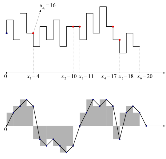
Figure 5. An example of a trajectory $l=(l_{i})_{i=1}^{20}$ with 6 beads is drawn on the upper picture. The auxiliary random walk $V$ associated with $l$, i.e., $(V_{i})_{i=0}^{21}=(T_{20})^{-1}(l)$ is drawn on the lower picture.

Auxiliary random walk

We display here the details of the proof of formula (1.36). Recall (1.4–1.7) and note that the $\widetilde{\wedge}$ operator can be written as

$$x\;\widetilde{\wedge}\;y=\left(|x|+|y|-|x+y|\right)/2,\quad\forall x,y\in\mathbb{Z}.$$ (2.1)

Hence, for $\beta>0$ and $L\in\mathbb{N}$, the partition function in (1.7) becomes

$$Z_{L,\beta} =\sum_{N=1}^{L}\sum_{\begin{subarray}{c}l\in\mathcal{L}_{N,L}\\ l_{0}=l_{N+1}=0\end{subarray}}\exp{\Bigl{(}\beta\sum_{n=1}^{N}{|l_{n}|}-\tfrac{\beta}{2}\sum_{n=0}^{N}{|l_{n}+l_{n+1}|}\Bigr{)}}$$

$$=c_{\beta}\,e^{\beta L}\sum_{N=1}^{L}\left(\tfrac{c_{\beta}}{e^{\beta}}\right)^{N}\sum_{\begin{subarray}{c}l\in\mathcal{L}_{N,L}\\ l_{0}=l_{N+1}=0\end{subarray}}\prod_{n=0}^{N}\frac{\exp{\Bigl{(}-\tfrac{\beta}{2}|l_{n}+l_{n+1}|\Bigr{)}}}{c_{\beta}},$$ (2.2)

where $c_{\beta}$ was defined in (1.13). At this stage, we pick $N\in\{1,\dots,L\}$ and we introduce the one-to-one correspondence $T_{N}:{\mathcal{V}}_{N+1,L-N}\mapsto{\mathcal{L}}_{N,L}$ defined as $T_{N}(V)_{i}=(-1)^{i-1}V_{i}$ for all $i\in\{1,\dots N\}$. We pick $l\in{\mathcal{L}}_{N,L}$, we consider $V=(T_{N})^{-1}(l)$ (see Fig. 5) and we note that the increments $(U_{i})_{i=1}^{N+1}$ of $V$ necessarily satisfy $U_{i}:=(-1)^{i-1}(l_{i-1}+l_{i})$. Thus, the partition function in (2.1) becomes

$$Z_{L,\beta}=c_{\beta}e^{\beta L}\sum_{N=1}^{L}\left(\tfrac{c_{\beta}}{e^{\beta}}\right)^{N}\sum_{V\in{\mathcal{V}}_{N+1,L-N}}\mathbf{P}_{\beta}(V),$$ (2.3)

which immediately implies (1.36). A useful consequence of formula (2.3) is that, once conditioned on taking a given number of horizontal steps $N$, the polymer measure is exactly the image measure by the $T_{N}$-transformation of the geometric random walk $V$ conditioned to return to the origin after N+1 steps and to make a geometric area $L-N$, i.e.,

$$P_{L,\beta}\bigl{(}l\in\cdot\mid N_{L}(l)=N\bigr{)}=\mathbf{P}_{\beta}\bigl{(}T_{N}(V)\in\cdot\mid V_{N+1}=0,A_{N}=L-N\bigr{)}.$$ (2.4)

From beads to excursions

We define $\Omega_{L}^{\mathsf{o}}$ as the subset of $\Omega_{L}$ containing those trajectories $l\in\Omega_{L}$ that have only one bead, i.e. $n_{L}(l)=1$. Thus, we can rewrite $\Omega^{\mathsf{o}}_{L}:=\bigcup_{N=1}^{L}\mathcal{L}^{\mathsf{o}}_{N,L}$, where $\mathcal{L}^{\mathsf{o}}_{N,L}$ is the subset of $\mathcal{L}_{N,L}$ defined as

$$\textstyle\mathcal{L}^{\mathsf{o}}_{N,L}=\bigl{\{}l\in\mathcal{L}_{N,L}\colon\,l_{i}\;\widetilde{\wedge}\;l_{i+1}\neq 0\ \forall i\in\{1,\dots,N-1\}\bigr{\}},$$ (2.5)

and we denote by $Z^{\mathsf{o}}_{L,\beta}$ the contribution to the partition function of those trajectories in $\Omega^{\mathsf{o}}_{L}$, i.e.,

$$Z^{\mathsf{o}}_{L,\beta}=\sum_{l\in\Omega_{L}^{\mathsf{o}}}e^{\beta H_{L}(l)}.$$ (2.6)

We let also $\mathcal{V}_{n,k}^{+}$ be the subset containing those trajectories that return to the origin after $n$ steps, satisfy $A_{n}=k$ and are strictly positive on $\{1,\dots,n\}$, i.e.,

$$\mathcal{V}_{n,k}^{+}:=\{V\colon\,V_{n}=0,\,A_{n}=k,\,V_{i}>0\ \forall i\in\{1,\dots,n-1\}\}.$$ (2.7)

By mimicking (2.1) and by noticing that by the $T_{N}$-transformation, the subset $\mathcal{L}^{\mathsf{o}}_{N,L}$ becomes $\mathcal{V}^{+}_{N+1,L-N}$ we obtain

$$Z^{\mathsf{o}}_{L,\beta}=2\,c_{\beta}\,e^{\beta L}\sum_{N=1}^{L}\left(\Gamma(\beta)\right)^{N}\mathbf{P}_{\beta}(\mathcal{V}^{+}_{N+1,L-N}).$$ (2.8)

2.2. Construction and regularity of $\mathfrak{h}_{\beta}$h

We define the function $\mathfrak{h}_{\beta}$ in a slightly different way from (1.14), but we will see at the end of this section that the two definitions are equivalent. For $N\in\mathbb{N},\delta\geq 0$, define

$$\mathfrak{h}_{N,\beta}(\delta):=\frac{1}{N}\log\mathbf{E}_{\beta}\bigl{(}e^{-\delta A_{N}}\mathbf{1}_{\{V_{N}=0\}}\bigr{)}\quad\text{and let}\quad\mathfrak{h}_{\beta}(\delta)=\lim_{N\to\infty}\mathfrak{h}_{N,\beta}(\delta).$$ (2.9)

Lemma 2.1.

(i) $\mathfrak{h}_{\beta}(\delta)$ exists and is finite, non-positive for all $\beta>0,\delta\geq 0$.
(ii) $\delta\mapsto\mathfrak{h}_{\beta}(\delta)$ is continuous, convex and non-increasing on $[0,\infty)$.

Proof.

(i) For $N,M\in\mathbb{N}$, we restrict the partition of size $N+M$ to those trajectories that return to the origin at time $N$ and use the Markov property to obtain

$$\mathbf{E}_{\beta}\bigl{(}e^{-\delta A_{N+M}}\mathbf{1}_{\{V_{N+M}=0\}}\bigr{)}\geq\mathbf{E}_{\beta}\bigl{(}e^{-\delta A_{N}}\mathbf{1}_{\{V_{N}=0\}}\bigr{)}\mathbf{E}_{\beta}\bigl{(}e^{-\delta A_{M}}\mathbf{1}_{\{V_{M}=0\}}\bigr{)}.$$ (2.10)

Thus, $\{\log\mathbf{E}_{\beta}\bigl{(}e^{-\delta A_{N}}\mathbf{1}_{\{V_{N}=0\}}\bigr{)}\}_{N\in\mathbb{N}}$ is a super-additive sequence that is bounded above by $0$ and therefore the limit in (2.9) exists, is finite and satisfies

$$\mathfrak{h}_{\beta}(\delta)=\sup_{N\in\mathbb{N}}\frac{1}{N}\log\mathbf{E}_{\beta}\bigl{(}e^{-\delta A_{N}}\mathbf{1}_{\{V_{N}=0\}}\bigr{)}\leq 0.$$ (2.11)

(ii) The fact that $A_{N}\geq 0$ for all $N\in\mathbb{N}$ immediately entails that $\delta\mapsto\mathfrak{h}_{\beta}(\delta)$ is non-increasing on $[0,\infty)$. By Hölder’s inequality, the function $\delta\mapsto\mathfrak{h}_{N,\beta}(\delta)$ is convex for all $N\in\mathbb{N}$ and hence so is $\delta\mapsto\mathfrak{h}_{\beta}(\delta)$. Convexity and finiteness imply continuity on $(0,\infty)$. In order to prove the continuity at $0$, we first note that $\lim_{\delta\to 0}\mathfrak{h}_{\beta}(\delta)=\sup_{\delta\geq 0}\mathfrak{h}_{\beta}(\delta)$. Then, with the help of formula 2.11 and via an exchange of suprema we obtain

$$\lim_{\delta\to 0}\mathfrak{h}_{\beta}(\delta) =\sup_{\delta\geq 0}\sup_{N\in\mathbb{N}}\frac{1}{N}\log\mathbf{E}_{\beta}\bigl{(}e^{-\delta A_{N}}\mathbf{1}_{\{V_{N}=0\}}\bigr{)}$$ (2.12)

$$=\sup_{N\in\mathbb{N}}\frac{1}{N}\log\mathbf{P}_{\beta}(V_{N}=0)=0.$$

∎

It remains to show that the two definitions of $\mathfrak{h}_{\beta}$ in (1.14) and (2.9) coincide. To that aim it suffices to show that

$$\limsup_{N\to\infty}\frac{1}{N}\log\mathbf{E}_{\beta}\bigl{(}e^{-\delta A_{N}}\bigr{)}\leq\lim_{N\to\infty}\frac{1}{N}\log\mathbf{E}_{\beta}\bigl{(}e^{-\delta A_{N}}\mathbf{1}_{\{V_{N}=0\}}\bigr{)}.$$ (2.13)

We set $\mathcal{I}_{N^{2}}:=[-N^{2},N^{2}]\cap\mathbb{Z}$  and we decompose $\mathbf{E}_{\beta}\bigl{(}e^{-\delta A_{N}}\bigr{)}$ into the two partition functions $C_{N,\beta}$ and $B_{N,\beta}$ defined as

$$C_{N,\beta}=\mathbf{E}_{\beta}\bigl{(}e^{-\delta A_{N}}\mathbf{1}_{\{V_{N}\in\mathcal{I}_{N^{2}}\}}\bigr{)}\quad\text{and}\quad B_{N,\beta}=\mathbf{E}_{\beta}\bigl{(}e^{-\delta A_{N}}\mathbf{1}_{\{V_{N}\notin\mathcal{I}_{N^{2}}\}}\bigr{)}.$$ (2.14)

Since $A_{N}\geq 0$ and since $\mathbf{E}_{\beta}{\left[{e^{\frac{\beta|U_{1}|}{4}}}\right]}<\infty$, Markov’s inequality gives

$$B_{N,\beta}\leq\mathbf{E}_{\beta}{\left[{\mathbf{1}_{\{V_{N}\notin\mathcal{I}_{N^{2}}\}}}\right]}\leq\mathbf{P}_{\beta}\Bigl{(}\sum_{i=1}^{N}|U_{i}|\geq N^{2}\Bigr{)}\leq\frac{\mathbf{E}_{\beta}{\left[{e^{\frac{\beta|U_{1}|}{4}}}\right]}^{N}}{e^{(\beta/4)N^{2}}},$$ (2.15)

which immediately implies that $\limsup_{N\to\infty}\frac{1}{N}\log B_{N,\beta}=-\infty$. Consequently

$$\limsup_{N\to\infty}\frac{1}{N}\log\mathbf{E}_{\beta}\bigl{(}e^{-\delta A_{N}}\bigr{)}=\limsup_{N\to\infty}\frac{1}{N}\log C_{N,\beta},$$ (2.16)

and since the cardinality of $\mathcal{I}_{N^{2}}$ grows polynomially, the proof of (2.13) will be complete once we show that

$$\limsup_{N\to\infty}\frac{1}{N}\log\sup_{x\in\mathcal{I}_{N^{2}}}\mathbf{E}_{\beta}\bigl{(}e^{-\delta A_{N}}\mathbf{1}_{\{V_{N}=x\}}\bigr{)}\leq\lim_{N\to\infty}\frac{1}{N}\log\mathbf{E}_{\beta}\bigl{(}e^{-\delta A_{N}}\mathbf{1}_{\{V_{N}=0\}}\bigr{)}.$$ (2.17)

For $x\in\mathbb{Z}$, we denote by $\mathbf{P}_{\beta,x}$ the law of $x+V$ where $V$ is the random walk of law $\mathbf{P}_{\beta}$. We consider the partition function of size $2N$ and use Markov property at time $N$ to obtain

$$\mathbf{E}_{\beta}\bigl{(}e^{-\delta A_{2N}}\mathbf{1}_{\{V_{2N}=0\}}\bigr{)}\geq\mathbf{E}_{\beta}\bigl{(}e^{-\delta A_{N}}\mathbf{1}_{\{V_{N}=x\}}\bigr{)}\mathbf{E}_{\beta,x}\bigl{(}e^{-\delta A_{N}}\mathbf{1}_{\{V_{N}=0\}}\bigr{)},\quad x\in\mathbb{Z}.$$ (2.18)

By using the time reversal property of the random walk $V$, we can assert that $(V_{N}-V_{N-n},\,0\leq n\leq N)\overset{d}{=}(V_{n}-V_{0},\,0\leq n\leq N)$ and consequently, for all $x\in\mathbb{Z}$, it comes that

$$\mathbf{E}_{\beta,x}\bigl{(}e^{-\delta\sum_{n=1}^{N}|V_{n}|}\mathbf{1}_{\{V_{N}=0\}}\bigr{)} =\mathbf{E}_{\beta}\bigl{(}e^{-\delta\sum_{n=1}^{N}|V_{n}+x|}\mathbf{1}_{\{V_{N}=-x\}}\bigr{)}$$

$$=\mathbf{E}_{\beta}\bigl{(}e^{-\delta\sum_{n=1}^{N}|V_{N}-V_{N-n}+x|}\mathbf{1}_{\{V_{N}=-x\}}\bigr{)}$$

$$=\mathbf{E}_{\beta}\bigl{(}e^{-\delta\sum_{n=1}^{N-1}|V_{n}|}\mathbf{1}_{\{V_{N}=-x\}}\bigr{)}.$$ (2.19)

Thanks to the symmetry of $V$ and since $\sum_{n=1}^{N-1}|V_{n}|\leq A_{N}$, the inequalities (2.18) and (2.2) allow us to write

$$\mathbf{E}_{\beta}\bigl{(}e^{-\delta A_{2N}}\mathbf{1}_{\{V_{2N}=0\}}\bigr{)}\geq\Big{[}\sup_{x\in\mathcal{I}_{N^{2}}}\mathbf{E}_{\beta}\bigl{(}e^{-\delta A_{N}}\mathbf{1}_{\{V_{N}=x\}}\bigr{)}\Big{]}^{2}.$$ (2.20)

It remains to apply $\frac{1}{2N}\log$ in both sides of (2.20) and to let $N\to\infty$ to obtain (2.17), which completes the proof.

2.3. Large deviation estimates

In this section, we introduce the techniques that will be required to estimate the probability of some large deviation events associated with trajectories making a large arithmetic area. Such estimates will be needed in Section 4 to approximate the probability that, under the polymer measure, the trajectories make only one bead.

Following Dobrushin and Hryniv in [DH96], for $n\in\mathbb{N}$, we define

$$Y_{n}:=\tfrac{1}{n}(V_{0}+V_{1}+\dots+V_{n-1}),$$ (2.21)

and for a given $q\in(0,\infty)\cap\tfrac{\mathbb{N}}{n}$, we focus on both probabilities $\mathbf{P}_{\beta}(Y_{n}=nq,\,V_{n}=0)$ and $\mathbf{P}_{\beta}(Y_{n}=nq,\,V_{n}=0,\,V_{i}>0\,\forall i\in\{1,\ldots,n-1\})$. Our aim is to identify the exponential rate at which such probabilities are decreasing and their asymptotic polynomial correction. To that aim, we will use an exponential tilting of the probability measure $\mathbf{P}_{\beta}$ (through the Cramer transform) in combination with a local limit theorem. Under the tilted probability measure the event $\{Y_{n}=nq,\,V_{n}=0\}$ is not of large deviation type anymore since its probability decays at polynomial speed instead of exponential speed, as will be seen in Section 6.

For the ease of notations, we set $\Lambda_{n}:=(Y_{n},V_{n})$ and we denote its logarithmic moment generating function by $\mathfrak{L}_{\Lambda_{n}}({\bf h})$ for ${\bf h}:=(h_{0},h_{1})\in\mathbb{R}^{2}$, i.e.,

$${\textstyle\mathfrak{L}_{\Lambda_{n}}({\bf h}):=\log\mathbf{E}_{\beta}\bigl{[}e^{h_{0}Y_{n}+h_{1}V_{n}}\bigr{]}=\sum_{i=1}^{n}\mathfrak{L}\Bigl{(}\bigl{(}1-\tfrac{i}{n}\bigr{)}h_{0}+h_{1}\Bigr{)}.}$$ (2.22)

Clearly, $\mathfrak{L}_{\Lambda_{n}}({\bf h})$ is finite for all ${\bf h}\in{\mathcal{D}}_{n}$ with

$${\textstyle\mathcal{D}_{n}:=\Bigl{\{}(h_{0},h_{1})\in\mathbb{R}^{2}\colon h_{1}\in\bigl{(}-\tfrac{\beta}{2},\tfrac{\beta}{2}\bigr{)},\ (1-\tfrac{1}{n})h_{0}+h_{1}\in\bigl{(}-\tfrac{\beta}{2},\tfrac{\beta}{2}\bigr{)}\Bigr{\}}.}$$ (2.23)

With the help of (6.24) and for ${\bf h}=(h_{0},h_{1})\in\mathcal{D}_{n}$, we define the ${\bf h}$-tilted distribution by

$$\frac{\text{d}\mathbf{P}_{n,{\bf h}}}{\text{d}\mathbf{P}_{\beta}}(V)=e^{h_{0}Y_{n}+h_{1}V_{n}-\mathfrak{L}_{\Lambda_{n}}(H)}.$$ (2.24)

For a given $n\in\mathbb{N}$ and $q\in\frac{\mathbb{N}}{n}$, the exponential tilt is given by ${\bf h}_{n}^{q}:=(h_{n,0}^{q},h_{n,1}^{q})$ which, by Lemma 5.4 in Section 5.1, is the unique solution of

$$\mathbf{E}_{n,{\bf h}}(\tfrac{\Lambda_{n}}{n})=\nabla\bigl{[}\tfrac{1}{n}\mathfrak{L}_{\Lambda_{n}}\bigr{]}(\mathbf{h})=(q,0),$$ (2.25)

and therefore, we have the equality

$$\mathbf{P}_{\beta}\bigl{(}\Lambda_{n}=(nq,0)\bigr{)}=\mathbf{P}_{n,{\bf h}_{n}^{q}}\bigl{(}\Lambda_{n}=(nq,0)\bigr{)}e^{n\big{(}-h_{n,0}^{q}\,q+\tfrac{1}{n}\mathfrak{L}_{\Lambda_{n}}({\bf h}_{n}^{q})\big{)}}.$$ (2.26)

From (2.26) it is easy to deduce that the exponential decay rate of $\mathbf{P}_{\beta}\bigl{(}\Lambda_{n}=(nq,0)\bigr{)}$ is given by the quantity $-h_{n,0}^{q}\,q+\frac{1}{n}\mathfrak{L}_{\Lambda_{n}}({\bf h}_{n}^{q})$ and that the polynomial correction is associated with $\mathbf{P}_{n,{\bf h}_{n}^{q}}\bigl{(}\Lambda_{n}=(nq,0)\bigr{)}$. To be more specific, we first state a Proposition which gives a local central limit theorem for the tilted law $\mathbf{P}_{n,{\bf h}_{n}^{q}}$.

Proposition 2.2.

For $[q_{1},q_{2}]\subset(0,\infty)$, there exist $C>0,n_{0}>0$ such that for all $q\in[q_{1},q_{2}]$ and $n\geq n_{0}$ we have

$$\tfrac{1}{Cn^{2}}\leq\mathbf{P}_{n,{\bf h}_{n}^{q}}(Y_{n}=nq,\,V_{n}=0)\leq\tfrac{C}{n^{2}}.$$ (2.27)

The following Proposition shows that the exponential decay rate induced by the change of probability in (2.24) can be controlled uniformly in $n$.

Proposition 2.3 (Decay rate of large area probability).

For $[q_{1},q_{2}]\subset(0,+\infty)$, there exist $c_{1},c_{2}>0$ and $n_{0}\in\mathbb{N}$ such that

$$\bigl{|}\bigl{[}\frac{1}{n}\mathfrak{L}_{\Lambda_{n}}({\bf h}_{n}^{q})-h_{n,0}^{q}\,q\bigr{]}-\bigl{[}\mathfrak{L}_{\Lambda}(\widetilde{\bf h}(q,0))-\widetilde{h}_{0}(q,0)\,q\bigr{]}\bigr{|}\leq\tfrac{c_{1}}{n},\quad\text{for}\ n\geq n_{0},\ q\in[q_{1},q_{2}].$$ (2.28)

and

$$\big{|}\big{|}{\bf h}_{n}^{q}-\widetilde{\bf h}(q,0)\big{|}\big{|}\leq\tfrac{c_{2}}{n},\quad\text{for}\ n\geq n_{0},\ q\in[q_{1},q_{2}].$$ (2.29)

Propositions 2.2 and 2.3 will be proven in Sections 6 and 5.1, respectively. With the help of (2.26) and by applying Proposition 2.2 and Proposition 2.3 we can finally give some sharp upper and lower bounds of $\mathbf{P}_{\beta}(Y_{n}=nq,\,V_{n}=0)$.

Proposition 2.4.

For $[q_{1},q_{2}]\subset(0,\infty)$, there exist $C_{1}>C_{2}>0$ and $n_{0}\in\mathbb{N}$ such that for all $q\in[q_{1},q_{2}]$ and $n\geq n_{0}$ we have

$$\tfrac{C_{2}}{n^{2}}\,e^{n\big{[}-\widetilde{h}_{0}(q,0)\,q+\mathfrak{L}_{\Lambda}(\widetilde{\bf h}(q,0))\big{]}}\leq\mathbf{P}_{\beta}(Y_{n}=nq,\,V_{n}=0)\leq\tfrac{C_{1}}{n^{2}}\,e^{n\big{[}-\widetilde{h}_{0}(q,0)\,q+\mathfrak{L}_{\Lambda}(\widetilde{\bf h}(q,0))\big{]}}.$$ (2.30)

In addition, we shall need in this paper a precise lower bound on the probability that, under $\mathbf{P}_{\beta}$, the random walk $V$ makes only one excursion away from the origin, conditionally on having a large prescribed area. To our knowledge, such an estimate is not available in the existing literature. Recall the definition of $Y_{n}$ in (2.21).

Proposition 2.5 (Unique excursion for large area).

For $[q_{1},q_{2}]\subset(0,\infty)$, there exist $C>0,\mu>0$ and $n_{0}\in\mathbb{N}$ such that for all $q\in[q_{1},q_{2}]$ and every $n\geq n_{0}$

$$\mathbf{P}_{\beta}\bigl{(}V_{i}>0,0<i<n\mid Y_{n}=nq,\,V_{n}=0\bigr{)}\geq\tfrac{C}{n^{\mu}}.$$ (2.31)

Although we can show that for the tilted law ${\bf P}_{n,{\bf h}_{n}^{q}}$ (thanks to the positive, respectively negative drifts of the increments close to $0$, resp. close to $n$) there exists a $C(q_{1},q_{2})>0$ so that for $q\in[q_{1},q_{2}]$ and $n$ large enough

$${\bf P}_{n,{\bf h}_{n}^{q}}\bigl{(}V_{i}>0,0<i<n\mid V_{n}=0\bigr{)}>C(q_{1},q_{2}),$$

and although we think that a similar result holds true for the l.h.s. in (2.31), we are unable to handle the conditioning by $Y_{n}=nq$ satisfactorily.

3. The order of the phase transition

In Section 3.1 below, we prove Theorem A that expresses the excess free energy as the solution of an equation involving the function $\mathfrak{h}_{\beta}$ introduced in Section 2.2. In Section 3.2, we first state Lemma 3.1 which provides the behavior of $\mathfrak{h}_{\beta}(\widetilde{f}(\beta))$ close to $\beta_{c}$ and then we combine this Lemma with Theorem A to complete the proof of Theorem B. Finally, in Section 3.3 we give a proof of Lemma 3.1.

3.1. Proof of Theorem A (Free energy equation)

By the representation formula (1.36) and the definition of $\widetilde{f}$, we have $\widetilde{f}(\beta)=\lim_{L\to\infty}\frac{1}{L}\log\widetilde{Z}_{L,\beta}$, where

$${\textstyle\widetilde{Z}_{L,\beta}:=\sum_{N=1}^{L}\left(\Gamma(\beta)\right)^{N}\mathbf{P}_{\beta}(\mathcal{V}_{N+1,L-N}).}$$ (3.1)

As a consequence, the excess free energy satisfies $\widetilde{f}(\beta)=-\log R$ where $R$ is the radius of convergence of the generating function $G(z)=\sum_{L=1}^{\infty}\widetilde{Z}_{L,\beta}\;z^{L}$, that is

$${\textstyle\widetilde{f}(\beta)=\sup\big{\{}\delta\geq 0\colon\sum_{L=1}^{\infty}\widetilde{Z}_{L,\beta}\;e^{-\delta L}=+\infty\big{\}},}$$ (3.2)

if the set is non-empty and $\widetilde{f}(\beta)=0$ otherwise. We recall (1.37) and we use (3.1) to rewrite the sum in (3.2) as

$$\sum_{L=1}^{\infty}\widetilde{Z}_{L,\beta}\;e^{-\delta L} =\sum_{L=1}^{\infty}\sum_{N=1}^{L}\bigl{(}\Gamma(\beta)e^{-\delta}\bigr{)}^{N}\sum_{\begin{subarray}{c}V_{0}=V_{N+1}=0\\ A_{N}=L-N\end{subarray}}\mathbf{P}_{\beta}(V)\,e^{-\delta(L-N)}$$

$$=\sum_{L=1}^{\infty}\sum_{N=1}^{L}\bigl{(}\Gamma(\beta)e^{-\delta}\bigr{)}^{N}\mathbf{E}_{\beta}\Bigl{(}e^{-\delta A_{N}}\mathbf{1}_{\{A_{N}=L-N,\,V_{N+1}=0\}}\Bigr{)}$$

$$=\sum_{N=1}^{\infty}\bigl{(}\Gamma(\beta)e^{-\delta}\bigr{)}^{N}\mathbf{E}_{\beta}\Bigl{(}e^{-\delta A_{N}}\mathbf{1}_{\{V_{N+1}=0\}}\Bigr{)}.$$ (3.3)

Since $A_{N}=A_{N+1}$ on the set $\{V_{N+1}=0\}$ and by using the definition of $\mathfrak{h}_{N,\beta}(\delta)$ in (2.9), the equality (3.1) becomes

$$\sum_{L=1}^{\infty}\widetilde{Z}_{L,\beta}\;e^{-\delta L}=\sum_{N=1}^{\infty}\exp{\Big{(}N\,\big{[}\log\Gamma(\beta)-\delta+\tfrac{N+1}{N}\,\mathfrak{h}_{N+1,\beta}(\delta)\big{]}\Big{)}},$$ (3.4)

which together with (3.2) gives ${\textstyle\widetilde{f}(\beta)=\sup\big{\{}\delta\geq 0\colon\log\Gamma(\beta)-\delta+\mathfrak{h}_{\beta}(\delta)>0\big{\}}.}$ Since $\mathfrak{h}_{\beta}(\delta)\leq 0$, it follows that $\widetilde{f}(\beta)=0$ if $\Gamma(\beta)\leq 1$. When $\Gamma(\beta)>1$, Lemma 2.1 gives that $\delta\mapsto-\delta+\mathfrak{h}_{\beta}(\delta)$ is continuous, decreasing, non-positive on $[0,\infty)$, equals $0$ at $\delta=0$ and tends to $-\infty$ when $\delta\to\infty$. Therefore, $\widetilde{f}(\beta)>0$ and is the unique solution of the equation $\log\Gamma(\beta)-\delta+\mathfrak{h}_{\beta}(\delta)=0$. In addition, by recalling the definition of the collapsed phase (1.11) and the extended phase (1.12), we can observe that

$$\mathcal{C}=\{\beta\colon\Gamma(\beta)\leq 1\}\quad\text{and}\quad\mathcal{E}=\{\beta\colon\Gamma(\beta)>1\}.$$ (3.5)

We note that $\beta\mapsto\Gamma(\beta)$ is decreasing on $[0,\infty)$ (recall (1.13) and (1.15)) and therefore, the collapse transition occurs at $\beta_{c}$, the unique positive solution of the equation $\Gamma(\beta)=1$.

3.2. Proof of Theorem B (Phase transition asymptotics)

We display here the proof of Theorem B subject to Lemma 3.1 below, that will be proven in Section 3.3 afterward.

Lemma 3.1.

$$\lim_{\beta\to\beta_{c}}\,\frac{\mathfrak{h}_{\beta}\bigl{(}\widetilde{f}(\beta)\bigr{)}}{\widetilde{f}(\beta)^{2/3}}=-\varsigma_{2}.$$ (3.6)

where we recall that $\varsigma_{2}$ was defined in (1.18).

Our aim is to study the asymptotic behavior of the equation in Theorem A near the critical point. We recall (1.15) and we perform a first order Taylor expansion of $\Gamma(\beta)$ near $\beta_{c}$ which gives $\log\Gamma(\beta_{c}-\varepsilon)=\varsigma_{1}\varepsilon(1+o(1))$ as $\varepsilon\searrow 0$. Next, we consider the function $\mathfrak{h}_{\beta}$ near $\beta_{c}$ and it follows from Lemma 3.1 that when $\varepsilon\searrow 0$

$$h_{\beta_{c}-\varepsilon}(\widetilde{f}(\beta_{c}-\varepsilon))=-\varsigma_{2}\widetilde{f}(\beta_{c}-\varepsilon)^{2/3}(1+o(1)).$$ (3.7)

Therefore, by plugging (3.7) and the expansion of $\log\Gamma(\beta_{c}-\varepsilon)$ in the equation in Theorem A that is verified by the excess free energy, we obtain that

$$\varsigma_{1}\varepsilon(1+o(1))-\widetilde{f}(\beta_{c}-\varepsilon)-\varsigma_{2}\widetilde{f}(\beta_{c}-\varepsilon)^{2/3}(1+o(1))=0,$$ (3.8)

which allows to conclude that

$$\widetilde{f}(\beta_{c}-\varepsilon)\sim\Bigl{(}\frac{\varsigma_{1}}{\varsigma_{2}}\Bigr{)}^{3/2}\,\varepsilon^{3/2}\quad\text{as}\ \ \varepsilon\searrow 0,$$ (3.9)

and the proof is complete.

3.3. Asymptotics of $\mathfrak{h}_{\beta}$h

Heuristics

Let us give the heuristic explanation of why $\mathfrak{h}_{\beta}(\delta)\sim-c\,\delta^{2/3}$ for some constant $c>0$. The main idea is to decompose the trajectory of the random walk $V$ into independent blocks of length $T\delta^{-2/3}$ for $T\in\mathbb{N}$ and $\delta$ small enough: we have approximately $N/(T\delta^{-2/3})$ such blocks. Hence, as $\delta\searrow 0$, we can estimate

$$\lim_{N\to\infty}\frac{1}{N}\log\mathbf{E}_{\beta}(e^{-\delta A_{N}})\sim\lim_{T\to\infty}\frac{\delta^{2/3}}{T}\log\mathbf{E}_{\beta}(e^{-\delta A_{T\delta^{-2/3}}}).$$ (3.10)

It is well known that for such random walks (assume that $\mathbf{E}_{\beta}(U_{1}^{2})=1$) (see [RD05, p. 405])

$$k^{-3/2}\sum_{i=1}^{Tk}|V_{i}|\xrightarrow{\mathcal{L}}\int_{0}^{T}|B(t)|dt\quad\text{as}\ k\to\infty,$$ (3.11)

where $B$ is a standard Brownian motion. Now, let $k=\delta^{-2/3}$ and since $|e^{-\delta A_{T\delta^{-2/3}}}|\leq 1$, we conclude that

$$\mathbf{E}_{\beta}(e^{-\delta A_{T\delta^{-2/3}}})\to\mathbf{E}(e^{-\int_{0}^{T}|B(t)|dt})\quad\text{as}\ \delta\to 0.$$ (3.12)

This convergence and (3.10) would immediately imply $\mathfrak{h}_{\beta}(\delta)\sim-c\,\delta^{2/3}$ where $c$ can be estimated via the distribution of the Brownian area, that is

$$c=-\lim_{T\to\infty}\frac{1}{T}\log\mathbf{E}(e^{-\int_{0}^{T}|B(t)|dt})>0.$$ (3.13)

Proof of Lemma 3.1.

Upper bound

Pick $T\in\mathbb{N}$, $\delta>0$ such that $\delta^{-2/3}\in\mathbb{N}$ and let $\Delta:=\delta^{-2/3}$. We take $N$ that satisfies $N/(T\Delta)\in\mathbb{N}$ and partition $\{1,\ldots,N\}$ into $k=N/(T\Delta)$ intervals of length $T\Delta$. By the Markov property of $V$, we decompose $\mathbf{E}_{\beta}\bigl{(}e^{-\delta A_{N}}\bigr{)}$ with respect to the position occupied by the random walk $V$ at times $T\Delta,2T\Delta,\ldots,(k-1)T\Delta$,

$$\mathbf{E}_{\beta}\bigl{(}e^{-\delta A_{N}}\bigr{)}=\sum_{\begin{subarray}{c}x_{0}=0,x_{i}\in\mathbb{Z}\\ i=1,\ldots,k\end{subarray}}\;\prod_{i=0}^{k-1}\mathbf{E}_{\beta,x_{i}}\Bigl{(}e^{-\delta A_{T\Delta}}\mathbf{1}_{\{V_{T\Delta}=x_{i+1}\}}\Bigr{)}\leq\Bigl{[}\;\sup_{x\in\mathbb{Z}}\mathbf{E}_{\beta,x}\bigl{(}e^{-\delta A_{T\Delta}}\bigr{)}\Bigr{]}^{k}.$$ (3.14)

With the help of Lemma 3.2 below, we can replace the supremum in the right hand side of (3.14) by the term indexed by $x=0$ only. The proof of Lemma 3.2 is postponed to Appendix B.

Lemma 3.2.

For all $\delta>0,n\in\mathbb{N}$ and $x,x^{\prime}\in\mathbb{Z}$ such that $|x^{\prime}|\geq|x|$, the following inequality holds true

$$\mathbf{E}_{\beta,x^{\prime}}\bigl{(}e^{-\delta A_{n}}\bigr{)}\leq\mathbf{E}_{\beta,x}\bigl{(}e^{-\delta A_{n}}\bigr{)}.$$ (3.15)

Therefore (3.14) becomes

$$\mathbf{E}_{\beta}\bigl{(}e^{-\delta A_{N}}\bigr{)}\leq\Bigl{[}\mathbf{E}_{\beta}\bigl{(}e^{-\delta A_{T\Delta}}\bigr{)}\Bigr{]}^{N/(T\Delta)}.$$ (3.16)

Recall that $\Delta:=\delta^{-2/3}$, apply $\frac{1}{N}\log$ to both sides of (3.16) and let $N\to\infty$ to obtain, for $\beta>0$ and $\delta>0$, that

$$\frac{\mathfrak{h}_{\beta}(\delta)}{\delta^{2/3}}\leq\frac{1}{T}\log\mathbf{E}_{\beta}\bigl{(}e^{-\delta A_{T\Delta}}\bigr{)}.$$ (3.17)

In what follows we need a uniform version (in $\beta$) of the convergence of $\mathbf{E}_{\beta}\bigl{(}e^{-\delta A_{T\Delta}}\bigr{)}$ towards $\mathbf{E}(e^{-\int_{0}^{T}|B(t)|dt})$ as $\delta\to 0$. For this reason, we introduce the strong approximation theorem (Sakhanenko [Sa80]) to approximate the partial sums of independent random variables $U$ in the right hand side in (3.17) by independent normal random variables.

Theorem 3.3 (Q. M. Shao [Sh95], Theorem B).

Denote by $\sigma_{\beta}^{2}$ the variance of the random variable $U_{1}$ under $\mathbf{P}_{\beta}$. We can redefine $\{U_{i},i\geq 1\}$ (denoted by $U^{\beta}$) on a richer probability space together with a sequence of independent standard normal random variables $\{X_{i},i\geq 1\}$ such that for every $p>2$, $x>0$,

$$\mathbf{P}\biggl{(}\max_{i\leq n}\,\biggl{|}\sum_{j=1}^{i}U^{\beta}_{j}-\sigma_{\beta}\sum_{j=1}^{i}X_{j}\biggr{|}\geq x\biggr{)}\leq(Ap)^{p}x^{-p}\sum_{i=1}^{n}\mathbf{E}|U^{\beta}_{i}|^{p},$$ (3.18)

where $A$ is an absolute positive constant.

We let also, for $n\in\mathbb{N}$, $Y_{n}=\sum_{i=1}^{n}X_{i}$, $A_{n}(Y)=\sum_{i=1}^{n}|Y_{i}|$ and redefine $V_{n}^{\beta}=\sum_{i=1}^{n}U_{i}^{\beta}$, $A_{n}(V^{\beta})=\sum_{i=1}^{n}|V_{i}^{\beta}|$. We pick $T>0$, $p>2$, $\vartheta>0$ and $K$ a compact subset of $(0,\infty)$. We use Theorem 3.3 and the fact that (recall (1.13)) $\mathbf{E}\bigl{[}|U_{1}^{\beta}|^{p}\bigr{]}$ is bounded from above uniformly in $\beta\in K$, to assert that there exists a constant $c_{p,K}>0$ such that for all $\Delta>0$ and $\beta\in K$

$$\mathbf{P}\Bigl{(}\,\max_{i\leq T\Delta}\,\bigl{|}V_{i}^{\beta}-\sigma_{\beta}Y_{i}\bigr{|}\geq\Delta^{\vartheta}\Bigr{)}\leq c_{p,K}\,T\,\Delta^{1-\vartheta p}.$$ (3.19)

Note that on the event $\{\max_{i\leq T\Delta}\,\bigl{|}V_{i}^{\beta}-\sigma_{\beta}Y_{i}\bigr{|}<\Delta^{\vartheta}\}$, we obviously have $|A_{T\Delta}(V^{\beta})-\sigma_{\beta}A_{T\Delta}(Y)|\leq T\Delta^{\vartheta+1}$. Therefore, since $x\mapsto\exp(-x)$ is 1-Lipschitz on $[0,\infty)$ and since $\Delta=\delta^{-2/3}$, we can write that for $\beta\in K$ and $\delta>0$

$$\bigl{|}\mathbf{E}\bigl{(}e^{-\delta A_{T\Delta}(V^{\beta})}-e^{-\delta\sigma_{\beta}A_{T\Delta}(Y)}\bigr{)}\bigr{|} \leq\mathbf{P}\Bigl{(}\,\max_{i\leq T\Delta}\,\bigl{|}V_{i}^{\beta}-\sigma_{\beta}Y_{i}\bigr{|}\geq\Delta^{\vartheta}\Bigr{)}+\delta T\Delta^{\vartheta+1}$$

$$\leq c_{p,K}T\delta^{\frac{2}{3}(\vartheta p-1)}+T\delta^{\frac{1}{3}(1-2\vartheta)}.$$ (3.20)

We chose $p=3$ and $\vartheta\in(1/3,1/2)$ and plug it in the right hand side of (3.17) to obtain that for $\beta\in K$ and $\delta>0$,

$$\frac{\mathfrak{h}_{\beta}(\delta)}{\delta^{2/3}}\leq\frac{1}{T}\log\Bigl{[}\mathbf{E}\bigl{(}e^{-\delta\sigma_{\beta}A_{T\Delta}(Y)}\bigr{)}+c_{3,K}T\delta^{\frac{2(3\vartheta-1)}{3}}+T\delta^{\frac{1-2\vartheta}{3}}\Bigr{]}.$$ (3.21)

Lemma 3.4.

Let K be a compact subset of $(0,+\infty)$. For $T>0$ and $\varepsilon>0$ there exists a $\delta_{0}>0$ such that for $\delta\leq\delta_{0}$ (with $\Delta=\delta^{-2/3}$),

$$\sup_{\beta\in K}\,\bigl{|}\mathbf{E}\bigl{(}e^{-\delta\sigma_{\beta}A_{T\Delta}(Y)}\bigr{)}-\mathbf{E}\bigl{(}e^{-\sigma_{\beta}\int_{0}^{T}|B(t)|dt}\bigr{)}\bigr{|}<\varepsilon,$$ (3.22)

where $B$ is a standard Brownian motion.

Proof of Lemma 3.4.

We can consider $\{B(t),t\geq 0\}$ and $\{y_{i},i\geq 1\}$ on the same probability space by letting $y_{i}=B(i)-B(i-1)$ and thus $Y_{i}:=y_{1}+\dots+y_{i}=B(i)$ for $i\in\mathbb{N}$. We recall that $A_{T\Delta}(Y)=\sum_{i=1}^{T\Delta}|B(i)|$ and therefore, by Brownian scaling we note that

$$\Delta^{-3/2}A_{T\Delta}(Y)\overset{d}{=}\Delta^{-1}\sum_{i=1}^{T\Delta}|B(i/\Delta)|.$$

Consequently, by recalling that $\delta=\Delta^{-3/2}$ we can replace $\mathbf{E}\bigl{(}e^{-\delta\sigma_{\beta}A_{T\Delta}(Y)}\bigr{)}$ in the left hand side of (3.22) by $\mathbf{E}\bigl{(}e^{-\sigma_{\beta}\Delta^{-1}\sum_{i=1}^{T\Delta}|B(i/\Delta)|}\bigr{)}$. Since the exponential function is 1-Lipschitz on $(-\infty,0]$, we have

$$\sup_{\beta\in K}\,\bigl{|}\mathbf{E}\bigl{(}e^{-\sigma_{\beta}\Delta^{-1}\sum_{i=1}^{T\Delta}|B(i/\Delta)|}\bigr{)} -\mathbf{E}\bigl{(}e^{-\sigma_{\beta}\int_{0}^{T}|B(t)|dt}\bigr{)}\bigr{|}$$ (3.23)

$${\textstyle\leq\max\{\sigma_{\beta},\beta\in K\}\ \mathbf{E}\Bigl{[}\bigl{|}\Delta^{-1}\sum_{i=1}^{T\Delta}|B(i/\Delta)|-\textstyle\int_{0}^{T}|B(t)|dt\bigr{|}\Bigr{]}}.$$

Since $\max\{\sigma_{\beta},\beta\in K\}<\infty$, since by Riemann sum approximation we know that

$$\Delta^{-1}\sum_{i=1}^{T\Delta}|B(i/\Delta)|\xrightarrow[\Delta\to\infty]{a.s.}\int_{0}^{T}|B(t)|dt,$$ (3.24)

and since we have uniform integrability (because $\sup_{\Delta>0}\mathbf{E}(|\Delta^{-1}\sum_{i=1}^{T\Delta}|B(i/\Delta)|^{2})<\infty$) we can conclude that

$$\lim_{\Delta\to\infty}\mathbf{E}\Bigl{[}\bigl{|}\Delta^{-1}\sum_{i=1}^{T\Delta}|B(i/\Delta)|-\textstyle\int_{0}^{T}|B(t)|dt\bigr{|}\Bigr{]}=0.$$ (3.25)

This completes the proof. ∎

We resume the proof of the upper bound. Since $\vartheta\in(1/3,1/2)$, the right hand side of (3.3) vanishes as $\delta\to 0$ uniformly in $\beta\in K$. Thus, we can replace $\delta$ by $\widetilde{f}(\beta_{c})$ in (3.21) and use Lemma 3.4 and the fact that $\lim_{\varepsilon\to 0^{+}}\widetilde{f}(\beta_{c}-\varepsilon)=0$ to conclude that, for all $T>0$,

$$\limsup_{\varepsilon\to 0^{+}}\frac{\mathfrak{h}_{\beta}(\widetilde{f}(\beta_{c}-\varepsilon))}{\widetilde{f}(\beta_{c}-\varepsilon)^{2/3}}\leq\frac{1}{T}\log\mathbf{E}\bigl{(}e^{-\sigma_{\beta_{c}}\int_{0}^{T}|B(t)|dt}\bigr{)}.$$ (3.26)

It remains to let $T$ tend to infinity and to recall (1.18) to obtain

$$\limsup_{\varepsilon\to 0^{+}}\frac{\mathfrak{h}_{\beta}(\widetilde{f}(\beta_{c}-\varepsilon))}{\widetilde{f}(\beta_{c}-\varepsilon)^{2/3}}\leq-\varsigma_{2}.$$ (3.27)

Lower bound

Recall that $T\in\mathbb{N},\delta>0$ and $\Delta=\delta^{-2/3}\in\mathbb{N}$. We also take $N\in\mathbb{N}$ such that $N/(T\Delta)\in\mathbb{N}$. Pick $\eta>0$ and use the decomposition in (3.14) to obtain

$$\mathbf{E}_{\beta}\bigl{(}e^{-\delta A_{N}}\bigr{)} \geq\sum_{\begin{subarray}{c}x_{0}=0,x_{i}\in[-\eta\sqrt{\Delta},\eta\sqrt{\Delta}]\\ i=1,\ldots,k\end{subarray}}\;\prod_{i=0}^{k-1}\mathbf{E}_{\beta,x_{i}}\Bigl{(}e^{-\delta A_{T\Delta}}\mathbf{1}_{\{V_{T\Delta}=x_{i+1}\}}\Bigr{)}$$ (3.28)

$$\geq\Bigl{[}\;\inf_{x\in[-\eta\sqrt{\Delta},\eta\sqrt{\Delta}]}\mathbf{E}_{\beta,x}\Bigl{(}e^{-\delta A_{T\Delta}}\mathbf{1}_{\{V_{T\Delta}\in[-\eta\sqrt{\Delta},\eta\sqrt{\Delta}]\}}\Bigr{)}\Bigr{]}^{N/(T\Delta)}.$$ (3.29)

For any integer $x\in[-\eta\sqrt{\Delta},\eta\sqrt{\Delta}]$, we consider the two sets of paths

$$\Pi_{1}^{x}=\bigl{\{}(V_{i})_{i=0}^{T\Delta}\colon V_{0}=x,\,V_{T\Delta}\in[-\eta\sqrt{\Delta},\eta\sqrt{\Delta}]\bigr{\}},$$ (3.30)

and

$$\Pi_{2}=\bigl{\{}(V_{i})_{i=0}^{T\Delta}\colon V_{0}=0,\,V_{T\Delta}\in[-\eta\sqrt{\Delta},0]\bigr{\}}.$$ (3.31)

Clearly, if $V=(V_{i})_{i=0}^{T\Delta}\in\Pi_{2}$, then the trajectory $V+x$ starts at $x\in[0,\eta\sqrt{\Delta}]$ and is an element of $\Pi_{1}^{x}$. Similarly, for $x\in[-\eta\sqrt{\Delta},0]$, $\Pi^{\prime}_{2}+x\subseteq\Pi_{1}^{x}$ where

$$\Pi^{\prime}_{2}=\bigl{\{}(V_{i})_{i=0}^{T\Delta}\colon V_{0}=0,\,V_{T\Delta}\in[0,\eta\sqrt{\Delta}]\bigr{\}}.$$ (3.32)

Since $\mathbf{P}_{\beta}(V\in\Pi_{2})=\mathbf{P}_{\beta}(V\in\Pi^{\prime}_{2})$, we conclude that

$$\mathbf{P}_{\beta,x}(V\in\Pi_{1}^{x})\geq\mathbf{P}_{\beta}(V\in\Pi^{\prime}_{2})\quad\text{for all}\;x\in[-\eta\sqrt{\Delta},\eta\sqrt{\Delta}].$$ (3.33)

Moreover, for any $V^{\star}\in\Pi_{1}^{x}$,

$$\delta\sum_{i=1}^{T\Delta}|V^{\star}_{i}|=\delta\sum_{i=1}^{T\Delta}|x+V_{i}|\leq\delta\sum_{i=1}^{T\Delta}|V_{i}|+\delta T\Delta|x|\leq\delta\sum_{i=1}^{T\Delta}|V_{i}|+\eta T,$$ (3.34)

where the trajectory $V$ satisfies $V_{0}=0$. Combining (3.33) and (3.34), we then have, for $x\in[-\eta\sqrt{\Delta},\eta\sqrt{\Delta}]$,

$$\mathbf{E}_{\beta,x}\Bigl{(}e^{-\delta A_{T\Delta}}\mathbf{1}_{\{V_{T\Delta}\in[-\eta\sqrt{\Delta},\eta\sqrt{\Delta}]}\Bigr{)}\geq e^{-\eta T}\mathbf{E}_{\beta}\Bigl{(}e^{-\delta A_{T\Delta}}\mathbf{1}_{\{V_{T\Delta}\in[0,\eta\sqrt{\Delta}]}\Bigr{)}.$$ (3.35)

By plugging the lower bound above into (3.28) and by using the symmetry of $V$ we immediately get

$$\mathbf{E}_{\beta}\bigl{(}e^{-\delta A_{N}}\bigr{)}\geq\Bigl{[}e^{-\eta T}\mathbf{E}_{\beta}\Bigl{(}e^{-\delta A_{T\Delta}}\mathbf{1}_{\{V_{T\Delta}\in\,[0,\eta\sqrt{\Delta}]\}}\Bigr{)}\Bigr{]}^{N/T\Delta},$$ (3.36)

which, by applying $\frac{1}{N}\log$ to both sides in (3.36) and by letting $N\to\infty$, gives, for all $\beta>0$,

$$\frac{\mathfrak{h}_{\beta}(\delta)}{\delta^{2/3}}\geq\frac{1}{T}\log\mathbf{E}_{\beta}\Bigl{(}e^{-\delta A_{T\Delta}}\mathbf{1}_{\{V_{T\Delta}\in[0,\eta\sqrt{\Delta}]\}}\Bigr{)}-\eta,\quad\delta,\eta>0.$$ (3.37)

At this stage, we proceed as in the upper bound (from (3.17)) to obtain, for all $T\in\mathbb{N},\eta>0$,

$$\liminf_{\beta\to\beta_{c}}\frac{\mathfrak{h}_{\beta}(\widetilde{f}(\beta))}{\widetilde{f}(\beta)^{2/3}}\geq\frac{1}{T}\log\mathbf{E}\bigl{(}e^{-\sigma_{\beta_{c}}\int_{0}^{T}|B(t)|dt}\mathbf{1}_{\{B(T)\in[0,\eta]\}}\bigr{)}-\eta.$$ (3.38)

It remains to show that for all $\eta>0$ we have

$$\lim_{T\to\infty}\frac{1}{T}\log\mathbf{E}\bigl{(}e^{-\sigma_{\beta_{c}}\int_{0}^{T}|B(t)|dt}\mathbf{1}_{\{B(T)\in[0,\eta]\}}\bigr{)}=\lim_{T\to\infty}\frac{1}{T}\log\mathbf{E}\bigl{(}e^{-\sigma_{\beta_{c}}\int_{0}^{T}|B(t)|dt}\bigr{)},$$ (3.39)

but the latter convergence can be obtained by adapting the proof of (2.13) to the continuous setting and for conciseness we will not give the details of the proof here. Then, by recalling (1.18), we achieve the bound

$$\liminf_{\beta\to\beta_{c}}\frac{\mathfrak{h}_{\beta}(\widetilde{f}(\beta))}{\widetilde{f}(\beta)^{2/3}}\geq-\varsigma_{2}-\eta,$$ (3.40)

for all $\eta>0$. It remains to let $\eta\to 0$ to complete the proof.

∎

4. Geometry of the collapsed phase

In Section 4.1 below, a proof of Theorem C is displayed subject to Lemma 4.1, which ensures that the horizontal extension of the polymer inside the collapsed phase is of order $\sqrt{L}$, and to Proposition 4.2, which provides a sharp estimate of the partition function restricted to those trajectories making only one bead. Proposition 4.2 is proven in Section 4.2 subject to Lemma 4.4, which is the counterpart of Lemma 4.1 for the one bead trajectory and to Proposition 2.5, which gives a lower bound on the probability that the random walk $V$ makes an $n$-step excursion away from the origin conditioned on the large deviation event $\{Y_{n}=qn,V_{n}=0\}$. Lemmas 4.1 and 4.4 are proven in Section 4.3 whereas the proof of Proposition 2.5 is postponed to Section 6.2 because it requires more preparation. Section 4.4 is dedicated to the proof of Theorem E and Section 4.5 to the proof of Theorem F.

4.1. Proof of Theorem C (One bead Theorem)

The proof of Theorem C will be displayed subject to Lemma 4.1 and Proposition 4.2 that are stated below.

Lemma 4.1.

For $\beta>\beta_{c}$, there exist $a,a_{1},a_{2}>0$ such that

$$P_{L,\beta}(N_{L}(l)\geq a_{1}\sqrt{L})\leq a_{2}\,e^{-a\sqrt{L}},\quad L\in\mathbb{N}.$$ (4.1)

Recall (2.6–2.8)

Proposition 4.2.

For $\beta>\beta_{c}$, there exist $c,c_{1},c_{2}>0$ and $\kappa>1/2$ such that

$$\frac{c_{1}}{L^{\kappa}}\,e^{\beta L-c\sqrt{L}}\leq Z_{L,\beta}^{\mathsf{o}}\leq\frac{c_{2}}{\sqrt{L}}\,e^{\beta L-c\sqrt{L}},\quad L\in\mathbb{N}.$$ (4.2)

Proof of Theorem C

We will first show that, for $\beta>\beta_{c}$ and under the polymer measure, the probability that there is exactly one macroscopic bead in the polymer tends to $1$ as $L\to\infty$. Then, we will show that, with a probability converging to $1$ as $L\to\infty$, the first step and the last step of this macroscopic bead are at distance less than $(\log L)^{4}$ from $0$ and $L$, respectively. For $r\in\mathbb{N}$, we denote by $Z_{L,\beta}[r]$ the partition function restricted to those trajectories that do not have any bead larger than $r$, i.e.,

$$Z_{L,\beta}[r]=\sum_{l\in\Omega_{L}\colon|I_{j_{\text{max}}}|\leq r}e^{\beta H_{L}(l)}.$$ (4.3)

At this stage, we pick $s>0$ and we let ${\mathcal{A}}_{L,s}$ be the subset consisting of those trajectories having at most one bead larger than $s(\log L)^{2}$, i.e.,

$${\mathcal{A}}_{L,s}=\Bigl{\{}l\in\Omega_{L}\colon\bigl{|}\bigl{\{}j\in\{1,\dots,n_{L}(l)\}\colon\,|I_{j}|\geq s(\log L)^{2}\bigr{\}}\bigr{|}\leq 1\Bigr{\}}.$$ (4.4)

Partition ${\mathcal{A}}_{L,s}^{c}$ with respect to the locations of the two subintervals $\{i_{1}+1,\dots,i_{2}\}$ and $\{i_{3}+1,\dots,i_{4}\}$ associated with the first two beads that are larger than $s(\log L)^{2}$. For notational convenience we let $L_{1}:=i_{2}-i_{1}$ and $L_{2}:=i_{4}-i_{3}$ be the length of these two first large beads. We do not have Markov property but, with the help of Lemma 4.3 below, we can estimate the partition function restricted to those trajectory that make a bead between two given steps.

Recall (cf. notations introduced in Section 1.3 prior to Theorem C) that $x_{1}$ denotes the horizontal extension of the first bead, and that $u_{x_{1}}$ corresponds to its total length.

Lemma 4.3.

For $L\in\mathbb{N}$,

$$\tfrac{1}{2}\,Z^{\mathsf{o}}_{L^{\prime},\beta}\,Z_{L-L^{\prime},\beta}\leq Z_{L,\beta}(u_{x_{1}}=L^{\prime})\leq Z^{\mathsf{o}}_{L^{\prime},\beta}\,Z_{L-L^{\prime},\beta}\quad\text{for}\;L^{\prime}\in\{1,\ldots,L\}.$$ (4.5)

Proof of Lemma 4.3.

In the case $u_{x_{1}}=1$, the first bead contains only one horizontal step, hence the sign of the stretch after $x_{1}$ is arbitrary, so that obviously $Z_{L,\beta}(u_{x_{1}}=1)=Z^{\mathsf{o}}_{1,\beta}Z_{L-1,\beta}$. In case $u_{x_{1}}=L^{\prime}>1$, note that the stretch $l_{x_{1}}$ is non-zero, therefore the next stretch has the same sign as $l_{x_{1}}$. By concatenating the trajectories

$$Z_{L,\beta}(u_{x_{1}}=L^{\prime}) =Z^{\mathsf{o}}_{L^{\prime},\beta}(l_{N_{L^{\prime}}}>0)Z_{L-L^{\prime},\beta}(l_{1}\geq 0)+Z^{\mathsf{o}}_{L^{\prime},\beta}(l_{N_{L^{\prime}}}<0)Z_{L-L^{\prime},\beta}(l_{1}\leq 0)$$ (4.6)

$$=Z^{\mathsf{o}}_{L^{\prime},\beta}\,Z_{L-L^{\prime},\beta}(l_{1}\geq 0).$$ (4.7)

In both cases, thanks to the symmetry of the stretches, we have

$$\tfrac{1}{2}\,Z^{\mathsf{o}}_{L^{\prime},\beta}\,Z_{L-L^{\prime},\beta}\leq Z_{L,\beta}(u_{x_{1}}=L^{\prime})\leq Z^{\mathsf{o}}_{L^{\prime},\beta}\,Z_{L-L^{\prime},\beta}\quad\text{for}\;L^{\prime}\in\{1,\ldots,L\}.$$ (4.8)

∎

We resume the proof of Theorem C and, we use Lemma 4.3 to obtain

$$P_{L,\beta}({\mathcal{A}}_{L,s}^{c})\leq\sum_{\stackrel{{\scriptstyle 1\leq i_{1}<i_{2}<i_{3}<i_{4}\leq L}}{{L_{1},L_{2}\geq s(\log L)^{2}}}}\frac{Z_{i_{1},\beta}\,\big{[}s(\log L)^{2}\big{]}\,Z_{L_{1},\beta}^{\mathsf{o}}\,Z_{i_{3}-i_{2},\beta}\big{[}s(\log L)^{2}\big{]}\,Z_{L_{2},\beta}^{\mathsf{o}}\,Z_{L-i_{4},\beta}}{Z_{L,\beta}},$$ (4.9)

and we write the lower bound

$$Z_{L,\beta}\geq(\tfrac{1}{2})^{3}Z_{i_{1},\beta}\big{[}s(\log L)^{2}\big{]}\,Z_{L_{1}+L_{2},\beta}^{\mathsf{o}}\,Z_{i_{3}-i_{2},\beta}\big{[}s(\log L)^{2}\big{]}Z_{L-i_{4},\beta}$$ (4.10)

such that

$$P_{L,\beta}({\mathcal{A}}_{L,s}^{c})\leq 8\sum_{\stackrel{{\scriptstyle 1\leq i_{1}<i_{2}<i_{3}<i_{4}\leq L}}{{L_{1},L_{2}\geq s(\log L)^{2}}}}\frac{Z_{L_{1},\beta}^{\mathsf{o}}\,Z_{L_{2},\beta}^{\mathsf{o}}}{Z_{L_{1}+L_{2},\beta}^{\mathsf{o}}}.$$ (4.11)

By using Proposition 4.2 and the convex inequality

$$\sqrt{L_{1}}+\sqrt{L_{2}}-\sqrt{L_{1}+L_{2}}\geq\tfrac{1}{2}\sqrt{\min\{L_{1},L_{2}\}},$$ (4.12)

we can bound from above the quantity in the sum in (4.11) by

$$\frac{Z_{L_{1},\beta}^{\mathsf{o}}Z_{L_{2},\beta}^{\mathsf{o}}}{Z_{L_{1}+L_{2},\beta}^{\mathsf{o}}} \leq\frac{c_{1}^{2}(L_{1}+L_{2})^{\kappa}}{c_{2}\sqrt{L_{1}L_{2}}}\;e^{-\widetilde{G}(a_{\beta})[\sqrt{L_{1}}+\sqrt{L_{2}}-\sqrt{L_{1}+L_{2}}]}$$ (4.13)

$$\leq\frac{c_{1}^{2}(L_{1}+L_{2})^{\kappa}}{c_{2}\sqrt{L_{1}L_{2}}}\;e^{-\tfrac{\widetilde{G}(a_{\beta})\sqrt{s}\log L}{2}}$$ (4.14)

and since $\frac{(L_{1}+L_{2})^{\kappa}}{\sqrt{L_{1}L_{2}}}\leq L^{\kappa}$ we can state that, for $L$ large enough, (4.11) becomes

$$P_{L,\beta}({\mathcal{A}}_{L,s}^{c})\leq\tfrac{8c_{1}^{2}}{c_{2}}\,L^{\kappa+4}e^{-\tfrac{\widetilde{G}(a_{\beta})\sqrt{s}\log L}{2}}.$$ (4.15)

Therefore, it suffices to choose $\sqrt{s}=\tfrac{4(\kappa+4)}{c}$ to conclude that $\lim_{L\to\infty}P_{L,\beta}({\mathcal{A}}_{L,s}^{c})=0$.

At this stage we set ${\mathcal{B}}_{L,s}={\mathcal{A}}_{L,s}\cap\{N_{L}(l)\leq a_{1}\sqrt{L}\}$ and we can use Lemma 4.1 and the fact that $P_{L,\beta}({\mathcal{A}}_{L,s}^{c})$ vanishes as $L\to\infty$ to conclude that $\lim_{L\to\infty}P_{L,\beta}({\mathcal{B}}_{L,s})=1$. Moreover, it comes easily that under the event ${\mathcal{B}}_{L,s}$ there is exactly one bead larger than $s(\log L)^{2}$ because if there were no bead larger than $s(\log L)^{2}$, then the total number of beads $n_{L}(l)$ would be larger than $\frac{L}{s(\log L)^{2}}$ which contradicts the fact that $N_{L}(l)\leq a_{1}\sqrt{L}$ because each bead contains at least one horizontal step and consequently $N_{L}(l)\geq n_{L}(l)$. Under the event ${\mathcal{B}}_{L,s}$ we denote by $i_{1}$ and $i_{2}$ the end-steps of the maximal bead, i.e., $I_{j_{\text{max}}}=\{i_{1}+1,\dots,i_{2}\}$. Then, the proof of Theorem C will be complete once we show that there exists a $v>0$ such that

$$\lim_{L\to\infty}P_{L,\beta}({\mathcal{B}}_{L,s}\cap\{i_{1}\geq v(\log L)^{4}\}) =0$$ (4.16)

$$\lim_{L\to\infty}P_{L,\beta}({\mathcal{B}}_{L,s}\cap\{i_{2}\leq L-v(\log L)^{4}\}) =0.$$ (4.17)

We can bound from above

$$P_{L,\beta}({\mathcal{B}}_{L,s}\cap\{i_{1}\geq v(\log L)^{4}\}) =\sum_{t=v(\log L)^{4}}^{L}P_{L,\beta}({\mathcal{B}}_{L,s}\cap\{i_{1}=t\})$$

$$\leq\sum_{t=v(\log L)^{4}}^{L}P_{L,\beta}\Big{(}\exists j\in\{1,\dots,n_{L}(l)\}\colon u_{x_{j}}=t,$$

$$\hskip 99.58464pt|I_{d}|\leq s(\log L)^{2}\quad\forall d\in\{1,\dots,j\}\Big{)}$$

$$\leq\tfrac{1}{2}\sum_{t=v(\log L)^{4}}^{L}\frac{Z_{t,\beta}[s(\log L)^{2}]\,Z_{L-t,\beta}}{Z_{t,\beta}\,Z_{L-t,\beta}},$$ (4.18)

which finally gives

$$P_{L,\beta}(B_{L,s}\cap\{i_{1}\geq v(\log L)^{4}\}) \leq\tfrac{1}{2}\sum_{t=v(\log L)^{4}}^{L}P_{t,\beta}\big{(}|I_{j_{\text{max}}}|\leq s(\log L)^{2}\big{)}.$$ (4.19)

We note that, under $P_{t,\beta}$ and on the event $\{|I_{j_{\text{max}}}|\leq s(\log L)^{2}\}$, the number of beads is larger than $\frac{t}{s(\log L)^{2}}$, therefore $N_{t}(l)\geq\frac{t}{s(\log L)^{2}}$ and since $\sqrt{t}\geq\sqrt{v}(\log L)^{2}$ we obtain that $N_{t}(l)\geq\sqrt{t}(\sqrt{v}/s)$. By choosing $v=(a_{1}s)^{2}$, we can apply Lemma 4.1 to get

$$P_{L,\beta}({\mathcal{B}}_{L,s}\cap\{i_{1}\geq v(\log L)^{4}\}) \leq\tfrac{1}{2}\sum_{t=v(\log L)^{4}}^{L}P_{t,\beta}\big{(}N_{t}(l)\geq a_{1}\sqrt{t}\big{)}$$

$$\leq\tfrac{1}{2}a_{2}\,\sum_{t=v(\log L)^{4}}^{L}e^{-a\sqrt{t}}.$$ (4.20)

Since the sum in (4.1) vanishes as $L\to\infty$, the proof is complete.

4.2. Proof of Proposition 4.2

We recall the definition of the one bead partition function introduced in Section 2.1, equations (2.5–2.8). Henceforth, we will use the notation $\widetilde{Z}_{L,\beta}^{\mathsf{o}}=Z_{L,\beta}^{\mathsf{m},\mathsf{o}}e^{-\beta L}/c_{\beta}$, so that Proposition 4.2 will be proven once we show that there exist $c_{1},c_{2}>0$ and $\kappa>1/2$ such that

$$\frac{c_{1}}{L^{\kappa}}\,e^{-\widetilde{G}(a_{\beta})\,\sqrt{L}}\leq\widetilde{Z}_{L,\beta}^{\mathsf{o}}\leq\frac{c_{2}}{\sqrt{L}}\,e^{-\widetilde{G}(a_{\beta})\,\sqrt{L}},\quad\text{for $L\in\mathbb{N}$ }.$$ (4.21)

We will prove (4.21) subject to Lemma 4.4 below and Proposition 2.5. The proof of Lemma 4.4 is given in Section 4.3 whereas the proof of Proposition 2.5 is postponed to Section 6.2. For $K\subset\{1,\dots,L\}$, we set

$$\widetilde{Z}^{\mathsf{o}}_{L,\beta}(N\in K)=2\sum_{N\in K}\left(\Gamma(\beta)\right)^{N}\mathbf{P}_{\beta}(\mathcal{V}^{+}_{N+1,L-N})\,,$$ (4.22)

and similarly we have

$$\widetilde{Z}^{\mathsf{o}}_{L,\beta}=2\sum_{N=1}^{L}\left(\Gamma(\beta)\right)^{N}\mathbf{P}_{\beta}(\mathcal{V}^{+}_{N+1,L-N}).$$ (4.23)

Lemma 4.4.

For $\beta>\beta_{c}$, there exists $a_{2}>a_{1}>0$ such that for $L\in\mathbb{N}$,

$$\lim_{L\to\infty}\frac{\widetilde{Z}^{\mathsf{o}}_{L,\beta}(a_{1}\sqrt{L}\leq N\leq a_{2}\sqrt{L})}{\widetilde{Z}^{\mathsf{o}}_{L,\beta}}=1.$$ (4.24)

By using Lemma 4.4, we note that it suffices to prove (4.21) with $\widetilde{Z}^{\mathsf{o}}_{L,\beta}\big{(}N\in\sqrt{L}\,[a_{1},a_{2}]\big{)}$ instead of $\widetilde{Z}^{\mathsf{o}}_{L,\beta}$. For the ease of notation, we will rather take $a_{2}$ a bit larger and consider $\widetilde{Z}^{\mathsf{o}}_{L,\beta}\big{(}1+N\in\sqrt{L}\,[a_{1},a_{2}]\big{)}$. In view of (4.22), we write

$$\textstyle\widetilde{Z}^{\mathsf{o}}_{L,\beta}\big{(}1+N\in\sqrt{L}\,[a_{1},a_{2}]\big{)}=2\sum_{N=a_{1}\sqrt{L}}^{a_{2}\sqrt{L}}\left(\Gamma(\beta)\right)^{N-1}\mathbf{P}_{\beta}(\mathcal{V}^{+}_{N,L-N+1}).$$ (4.25)

For $n\in\mathbb{N}$, we recall (1.37) and (2.21) and we note that $nY_{n}=A_{n}$ on the set $\{V_{n}=0,\,V_{i}>0\ \forall i\in[1,N-1]\cap\mathbb{N}\}$. Therefore, we set $q_{N,L}:=\frac{L-N+1}{N^{2}}$ for $N\in\sqrt{L}[a_{1},a_{2}]\cap\mathbb{N}$ and we can write

$$\mathcal{V}^{+}_{N,L-N+1}=\{V\colon Y_{N}=Nq_{N,L},\,V_{N}=0,\,V_{i}>0\ \forall i\in[1,N-1]\cap\mathbb{N}\}.$$ (4.26)

At this stage, our aim is to bound from above and below the quantities $\mathbf{P}_{\beta}(\mathcal{V}^{+}_{N,L-N+1})$ for $N\in\sqrt{L}[a_{1},a_{2}]\cap\mathbb{N}$. The upper bound is obvious, i.e.,

$$\mathbf{P}_{\beta}(\mathcal{V}^{+}_{N,L-N+1})\leq\mathbf{P}_{\beta}(Y_{N}=Nq_{N,L},\,V_{N}=0),$$ (4.27)

while the lower bound is obtained as follows. Since $q_{N,L}\in\bigl{[}\frac{1}{2a_{2}^{2}},\frac{1}{a_{1}^{2}}\bigr{]}$ when $N\in\sqrt{L}[a_{1},a_{2}]$, we can apply Proposition 2.5 to claim that, there exists $C,\mu>0$ such that for $L$ large enough,

$$\mathbf{P}_{\beta}(\mathcal{V}^{+}_{N,L-N+1})\geq\tfrac{C}{N^{\mu}}\mathbf{P}_{\beta}(Y_{N}=Nq_{N,L},\,V_{N}=0),\quad N\in\sqrt{L}[a_{1},a_{2}]\cap\mathbb{N}.$$ (4.28)

By using again the fact that $q_{N,L}\in\bigl{[}\frac{1}{2a_{2}^{2}},\frac{1}{a_{1}^{2}}\bigr{]}$ when $N\in\sqrt{L}\,[a_{1},a_{2}]$, we can apply Proposition 2.4, which provides a lower and an upper bound on $\mathbf{P}_{\beta}(Y_{N}=Nq_{N,L},\,V_{N}=0)$. By combining these last two bounds with (4.27–4.28) and by setting $\kappa=1+\mu/2$ we can assert that there exists $R_{1}>R_{2}>0$ such that for $L$ large enough and all $N\in\sqrt{L}\,[a_{1},a_{2}]$ we have that

$$\tfrac{R_{2}}{L^{\kappa}}\, e^{N\big{[}-\widetilde{h}_{0}(q_{N,L},0)\,q_{N,L}+\mathfrak{L}_{\Lambda}(\widetilde{\bf h}(q_{N,L},0))\big{]}}$$ (4.29)

$$\hskip 56.9055pt\leq\mathbf{P}_{\beta}({\mathcal{V}}^{+}_{N,L-N+1})\leq\tfrac{R_{1}}{L}\,e^{N\big{[}-\widetilde{h}_{0}(q_{N,L},0)\,q_{N,L}+\mathfrak{L}_{\Lambda}(\widetilde{\bf h}(q_{N,L},0))\big{]}}.$$

At this stage, we recall the definition of $\widetilde{G}$ in (1.27) and we set

$$Q_{L,\beta}:=\sum_{N=a_{1}\sqrt{L}}^{a_{2}\sqrt{L}}e^{\sqrt{L}\,G_{L,N}}$$ (4.30)

with

$$G_{L,N}=\tfrac{N}{\sqrt{L}}\,\big{(}q_{N,L}\big{)}^{1/2}\,\widetilde{G}\Big{(}\tfrac{1}{(q_{N,L})^{1/2}}\Big{)}$$ (4.31)

and we use (4.22) and (4.29) to claim that there exists $R_{3}>R_{4}>0$ (depending on $\beta$ only) such that for $L$ large enough,

$$\tfrac{R_{4}}{L^{\kappa}}\,Q_{L,\beta}\leq\widetilde{Z}^{\mathsf{o}}_{L,\beta}\big{(}N\in\sqrt{L}\,[a_{1},a_{2}]\big{)}\leq\tfrac{R_{3}}{L}\,Q_{L,\beta}.$$ (4.32)

We recall that $a\mapsto\widetilde{G}(a)$ is a strictly negative and strictly concave function on $(0,\infty)$ and reaches its unique maximum at $a_{\beta}$, which obviously belongs to $[a_{1},a_{2}]$. Since, by Lemma 5.3, $a\mapsto\widetilde{G}(a)$ is $\mathcal{C}^{1}$ on $(0,\infty)$, we can assert that it is Lipschitz on each compact subset of $(0,\infty)$. Moreover, there exists a $C>0$ such that $|q_{N+1,L}-q_{N,L}|\leq C/\sqrt{L}$ for $N\in\sqrt{L}\,[a_{1},a_{2}]$ and we have that

$${\textstyle\Big{(}1-\frac{a_{2}}{\sqrt{L}}\Big{)}^{\frac{1}{2}}\leq\tfrac{N}{\sqrt{L}}\,(q_{N,L})^{\frac{1}{2}}\leq\Big{(}1-\frac{a_{1}}{\sqrt{L}}\Big{)}^{\frac{1}{2}}},\quad N\in\sqrt{L}[a_{1},a_{2}],$$ (4.33)

therefore, we can take the supremum of $G_{L,N}$ on $N\in\bigl{[}a_{1}\sqrt{L},a_{2}\sqrt{L}\,\bigr{]}\cap\mathbb{N}$ and it comes that

$$\sup\big{\{}G_{L,N};\,N\in\sqrt{L}\,[a_{1},a_{2}]\cap\mathbb{N}\big{\}}=\widetilde{G}(a_{\beta})+O(\tfrac{1}{\sqrt{L}}).$$ (4.34)

By putting together (4.30) and (4.34) we obtain that there exists $R_{5}>R_{6}>0$ such that for L large enough,

$$R_{6}\,e^{\widetilde{G}(a_{\beta})\sqrt{L}}\leq Q_{L,\beta}\leq R_{5}\sqrt{L}\,e^{\widetilde{G}(a_{\beta})\sqrt{L}}.$$ (4.35)

At this stage it suffices to combine (4.32) with (4.35) to complete the proof of (4.21) with $\kappa=\mu/2+1$.

4.3. Proof of Lemmas 4.1 and 4.4

We will only display the proof of Lemma 4.4 because the proof of Lemma 4.1 is obtained in a very similar manner. We recall (4.22) and (4.23) and we will first show that there exists $\gamma>0$ and $c>0$ such that

$$\widetilde{Z}_{L,\beta}^{\mathsf{o}}\geq c\,e^{-\gamma\sqrt{L}},\quad L\in\mathbb{N}.$$ (4.36)

Then, we will show that there exist $a_{2}>a_{1}>0$ and $c_{1},c_{2}>0$ such that

$$\widetilde{Z}_{L,\beta}^{\mathsf{o}}(N\geq a_{2}\sqrt{L}) \leq c_{2}\,e^{-2\gamma\sqrt{L}},\quad L\in\mathbb{N},$$

$$\widetilde{Z}_{L,\beta}^{\mathsf{o}}(N\leq a_{1}\sqrt{L}) \leq c_{1}\,e^{-2\gamma\sqrt{L}},\quad L\in\mathbb{N}.$$ (4.37)

Putting together (4.36) and (4.3), we will immediately obtain (4.24). To begin with, set $r:=\Big{\lfloor}\tfrac{L}{1+\lfloor\sqrt{L}\rfloor}\Big{\rfloor}$, $u:=L-r-(r-1)\lfloor\sqrt{L}\rfloor$ and note that $u\in\{\lfloor\sqrt{L}\rfloor,\dots,2\lfloor\sqrt{L}\rfloor\}$. Then, consider the trajectory $V^{*}\in\mathcal{V}_{r+1,L-r}^{+}$ defined as $V_{0}=V_{r+1}=0$, $V_{1}=\dots=V_{r-1}=\lfloor\sqrt{L}\rfloor$ and $V_{r}=u$. One can therefore compute

$$\mathbf{P}_{\beta}(V^{*})=\big{(}\tfrac{1}{c_{\beta}}\big{)}^{r+1}e^{-\tfrac{\beta}{2}(2u)}\geq\big{(}\tfrac{1}{c_{\beta}}\big{)}^{r+1}e^{-2\beta\lfloor\sqrt{L}\rfloor},$$ (4.38)

and consequently by restricting the sum in (4.22) to $N=r$, by using (4.38) and the inequality $\lfloor\sqrt{L}\rfloor\leq\sqrt{L}$, we obtain

$$\widetilde{Z}_{L,\beta}^{\mathsf{o}}\geq\tfrac{2}{c_{\beta}}\left(\tfrac{\Gamma(\beta)}{c_{\beta}}\right)^{r}\ e^{-2\beta\sqrt{L}}.$$ (4.39)

It remains to note that $r\leq\sqrt{L}$ and to recall that $c_{\beta}>1$ and that $\Gamma(\beta)<1$ because $\beta>\beta_{c}$. This is sufficient to obtain (4.36).

Proving the first inequality in (4.3) is easy because $\Gamma(\beta)<1$ and thus, we can use (4.22) to claim that there exists a $C>0$ such that

$$\widetilde{Z}^{\mathsf{o}}_{L,\beta}(N\geq a_{2}\sqrt{L})\leq 2\sum_{N=a_{2}\sqrt{L}}^{\infty}\left(\Gamma(\beta)\right)^{N}\leq Ce^{a_{2}\log(\Gamma(\beta))\sqrt{L}}.$$ (4.40)

Since $\log(\Gamma(\beta))<0$, it suffices to choose $a_{2}$ large enough to obtain the first inequality in (4.3).

To prove the last inequality in (4.3), we note that, for $N\leq a_{1}\sqrt{L}$ and for all $(V_{i})_{i=0}^{N+1}\in\mathcal{V}^{+}_{N+1,L-N}$ we have $\max\{V_{j},\,j\in\{1,\dots,N\}\}\geq\frac{L-N}{N}\geq\frac{\sqrt{L}}{a_{1}}-1$ and therefore, for $L$ large enough we have

$$\mathbf{P}_{\beta}(\mathcal{V}^{+}_{N+1,L-N}) \leq\mathbf{P}_{\beta}\Big{(}\max\{V_{j},j\leq a_{1}\sqrt{L}\}\geq\tfrac{\sqrt{L}}{2a_{1}}\Big{)}$$ (4.41)

$$\leq\textstyle\mathbf{P}_{\beta}\Big{(}\sum_{i=1}^{a_{1}\sqrt{L}}|U_{i}|>\tfrac{\sqrt{L}}{2a_{1}}\Big{)},$$ (4.42)

and since $U_{1}$ has some finite exponential moments, we can apply a standard Cramer’s Theorem to obtain that for $L$ large enough, there exists $g(a_{1})>0$ such that $\lim_{a_{1}\to 0^{+}}g(a_{1})=\infty$ and that $\mathbf{P}_{\beta}(\mathcal{V}^{+}_{N+1,L-N})\leq e^{-g(a_{1})\sqrt{L}}$ for $N\leq a_{1}\sqrt{L}$. Therefore, by taking $a_{1}$ small enough we obtain the second inequality in (4.3), which completes the proof of Lemma 4.4.

4.4. Proof of Theorem E (Horizontal extension)

To begin this section, we prove that $\widetilde{G}$ is strictly concave and reaches its maximum at a unique point $a_{\beta}\in(0,\infty)$. Recall (1.27) and compute its first two derivatives (by using that $\nabla\mathfrak{L}_{\Lambda}(\widetilde{\bf h}(q,0))=(q,0)$), i.e.,

$$\frac{d}{da}\widetilde{G}(a) =\log\Gamma(\beta)+\tfrac{1}{a^{2}}\widetilde{h}_{0}\bigl{(}\tfrac{1}{a^{2}},0\bigr{)}+\mathfrak{L}_{\Lambda}(\widetilde{\bf h}(\tfrac{1}{a^{2}},0)),$$ (4.43)

$$\frac{d^{2}}{da^{2}}\widetilde{G}(a) =-\tfrac{2}{a^{3}}\widetilde{h}_{0}\bigl{(}\tfrac{1}{a^{2}},0\bigr{)}-\tfrac{4}{a^{5}}\partial_{1}\widetilde{h}_{0}\bigl{(}\tfrac{1}{a^{2}},0\bigr{)}.$$ (4.44)

It suffices to show that $\frac{d^{2}}{da^{2}}\widetilde{G}(a)<0$ on $(0,\infty)$ and that $\frac{d}{da}\widetilde{G}(a)$ has a zero on $(0,\infty)$. Since $\widetilde{h}_{0}(x,0)=-2\widetilde{h}_{1}(x,0)$ (recall Remark 5.5), we consider $R:u\mapsto\int_{0}^{1}x\mathfrak{L}^{\prime}((x-\tfrac{1}{2})u)dx$ so that $\partial_{1}(\mathfrak{L}_{\Lambda})(\widetilde{\bf h}(x,0))=R(\widetilde{h}_{0}(x,0))$. Clearly $R(0)=0$ and $R^{\prime}(u)=2\int_{0}^{1}x^{2}\mathfrak{L}^{\prime\prime}(xu)dx$ because $\mathfrak{L}$ is even (recall (1.23)). Therefore $R^{\prime}(u)>0$ when $u\neq 0$ and $R<0$ on $(-\infty,0)$ and $R>0$ on $(0,\infty)$. Since $R(\widetilde{h}_{0}(x,0))=x$ for $x\in\mathbb{R}$, we can claim that $\widetilde{h}_{0}(x,0)>0$ for $x\in(0,\infty)$ and by differentiating this latter equality we obtain that $\partial_{1}\widetilde{h}_{0}(x,0)=1/R^{\prime}(\widetilde{h}_{0}(x,0))$ which is strictly positive on $(0,\infty)$. This completes the proof.

Let us start the proof of Theorem E. Recall that $i_{1}$ and $i_{2}$ are the end-steps of the largest bead $I_{j_{\text{max}}}$, i.e., $I_{j_{\text{max}}}=\{i_{1}+1,\dots,i_{2}\}$. For $v>0$, we let

$${\mathcal{T}}_{L,v}:=\bigl{\{}l\in\Omega_{L}\colon i_{1}\leq v(\log L)^{4},\,i_{2}\geq L-v(\log L)^{4},\,I_{j_{\text{max}}}=\{i_{1}+1,\dots,i_{2}\}\bigr{\}}.$$ (4.45)

By Theorem C, there exists a $v>0$ such that $\lim_{L\to\infty}P_{L,\beta}({\mathcal{T}}_{L,v})=1$. Therefore, the proof will be complete once we show that

$$\lim_{L\to\infty}P_{L,\beta}\biggl{(}\Bigl{\{}\Bigl{|}\frac{N_{L}(l)}{\sqrt{L}}-a_{\beta}\Bigr{|}>\varepsilon\Bigr{\}}\cap{\mathcal{T}}_{L,v}\biggr{)}=0.$$ (4.46)

Let $N_{I_{j_{\text{max}}}}$ denote the number of horizontal steps made by the random walk in its largest bead. Pick $\varepsilon^{\prime}<\varepsilon$ and since the first step and the last step of the largest bead are at distance less than $v(\log L)^{4}$ from $0$ and $L$, respectively, we can write that for $L$ large enough

$$P_{L,\beta}\biggl{(}\Bigl{\{}\Bigl{|}\frac{N_{L}(l)}{\sqrt{L}}-a_{\beta}\Bigr{|}>\varepsilon\Bigr{\}}\cap{\mathcal{T}}_{L,v}\biggr{)}$$

$$\leq\sum_{\begin{subarray}{c}1\leq i_{1}\leq v(\log L)^{4}\\ L-v(\log L)^{4}\leq i_{2}\leq L\end{subarray}} P_{L,\beta}\biggl{(}\Bigl{|}\tfrac{N_{I_{j_{\text{max}}}}}{\sqrt{i_{2}-i_{1}}}-a_{\beta}\Bigr{|}>\varepsilon^{\prime},\,I_{j_{\text{max}}}=\{i_{1}+1,\dots,i_{2}\}\biggr{)}$$

$$\leq 4\sum_{\begin{subarray}{c}1\leq i_{1}\leq v(\log L)^{4}\\ L-v(\log L)^{4}\leq i_{2}\leq L\end{subarray}}\frac{Z^{\mathsf{o}}_{i_{2}-i_{1},\beta}\biggl{(}\Bigl{|}\tfrac{N}{\sqrt{i_{2}-i_{1}}}-a_{\beta}\Bigr{|}>\varepsilon^{\prime}\biggr{)}}{Z^{\mathsf{o}}_{i_{2}-i_{1},\beta}},$$ (4.47)

where the coefficient $4$ in front of the r.h.s. in (4.4) comes from a direct application of Lemma 4.3. Now, we focus on the numerator of the r.h.s. in (4.4) and since $\widetilde{G}$ is strictly concave and reaches its maximum at $a_{\beta}$ we can claim that the maximum of $\widetilde{G}$ on $(0,a_{\beta}-\varepsilon^{\prime}]\cup[a_{\beta}+\varepsilon^{\prime},\infty)$ is given by $T(\varepsilon^{\prime})=\max\{\widetilde{G}(a_{\beta}-\varepsilon^{\prime}),\widetilde{G}(a_{\beta}+\varepsilon^{\prime})\}$. We proceed as in (4.25)-(4.34) and we get that there exits a $C_{1}>0$ such that

$$Z^{\mathsf{o}}_{i_{2}-i_{1},\beta}\biggl{(}\Bigl{|}\tfrac{N}{\sqrt{i_{2}-i_{1}}}-a_{\beta}\Bigr{|}>\varepsilon^{\prime}\biggr{)}\leq\tfrac{C_{1}}{\sqrt{i_{2}-i_{1}}}\,e^{\beta(i_{2}-i_{1})}\,e^{T(\varepsilon^{\prime})\sqrt{i_{2}-i_{1}}}.$$ (4.48)

We apply Proposition 4.2 and the denominator can be bounded from below as

$$Z^{\mathsf{o}}_{i_{2}-i_{1},\beta}\geq\tfrac{C_{2}}{(i_{2}-i_{1})^{\kappa}}\,e^{\beta(i_{2}-i_{1})}\,e^{\widetilde{G}(a_{\beta})\sqrt{i_{2}-i_{1}}},$$ (4.49)

for some constants $\kappa>1/2$ and $C_{2}>0$. Since $L-2v(\log L)^{4}\leq i_{2}-i_{1}\leq L$, we can state that, for $L$ large enough, (4.4) becomes

$$P_{L,\beta}\biggl{(}\Bigl{\{}\Bigl{|}\frac{N_{L}(l)}{\sqrt{L}}-a_{\beta}\Bigr{|}>\varepsilon\Bigr{\}}\cap\,{\mathcal{T}}_{L,v}\biggr{)}\leq C_{3}\,L^{\kappa-\frac{1}{2}}\,\log(L)^{8}\,e^{-(\widetilde{G}(a_{\beta})-T(\varepsilon^{\prime}))\sqrt{L-2v(\log L)^{4}}}.$$ (4.50)

Since $\widetilde{G}(a_{\beta})>T(\varepsilon^{\prime})$, the right hand side vanishes as $L\to\infty$ and this completes the proof.

4.5. Proof of Theorem F (Wulff shape)

Before displaying the proof of Theorem F, we provide a rigorous definition of $\gamma^{*}_{\beta}$ and we associate with each trajectory $l\in\Omega_{L}$ the process $M_{l}$ that links the middle of each stretch consecutively.

The Wulff shape $\gamma^{*}_{\beta}$ can be defined as

$$\gamma^{*}_{\beta}=\text{argmin}\big{\{}J(\gamma),\,\gamma\in{\mathcal{B}}_{[0,1]},\,{\textstyle\int_{0}^{1}\gamma(t)dt}=\tfrac{1}{a_{\beta}^{2}},\gamma(0)=\gamma(1)=0\big{\}},$$ (4.51)

where ${\mathcal{B}}_{[0,1]}$ is the set containing the cadlag real functions defined on $[0,1]$, where $J:{\mathcal{B}}_{[0,1]}\to[0,\infty]$ is defined as

$$J(\gamma)=\begin{dcases*}\int_{0}^{1}\mathfrak{L}^{*}(\gamma^{\prime}(t))dt\quad\text{if}\quad\gamma\in{\mathcal{A}}{\mathcal{C}},\\ +\infty\quad\text{otherwise},\end{dcases*}$$ (4.52)

where ${\mathcal{A}}{\mathcal{C}}$ is the set of absolutely continuous functions and where $\mathfrak{L}^{*}$ is the Legendre transform of $\mathfrak{L}$, i.e.,

$$\mathfrak{L}^{*}(u)=\sup\big{\{}hu-\mathfrak{L}(h),h\in(-\tfrac{\beta}{2},\tfrac{\beta}{2})\big{\}},\quad u\in\mathbb{R}.$$ (4.53)

Using the duality between $\mathfrak{L}$ and $\mathfrak{L}^{*}$ we easily obtain the formula (1.28) given in the introduction, which easily implies (recall 1.27) that $\widetilde{G}(a_{\beta})=a_{\beta}(\log\Gamma(\beta)-J(\gamma^{*}_{\beta}))$. Finally, we note that one can prove without further difficulty that

$$\{-\gamma^{*}_{\beta},\gamma^{*}_{\beta}\}=\text{argmin}\big{\{}J(\gamma),\,\gamma\in{\mathcal{B}}_{[0,1]},\,A(\gamma)=\tfrac{1}{a_{\beta}^{2}},\gamma(0)=\gamma(1)=0\big{\}},$$ (4.54)

where $A(\gamma):=\int_{0}^{1}|\gamma(s)|ds$ is the geometric area enclosed between the graph of $\gamma$ and the $x$-axis.

We recall the definition of ${\mathcal{E}}_{l}^{+}$ and ${\mathcal{E}}_{l}^{-}$ in (1.32) and we also associate with each $l\in{\mathcal{L}}_{N,L}$ the path $M_{l}=\big{(}M_{l,i}\big{)}_{i=0}^{N+1}$ that links the middles of each stretch consecutively and is defined as $M_{l,0}=0$

$$M_{l,i}=l_{1}+\dots+l_{i-1}+\frac{l_{i}}{2},\quad i\in\{1,\dots,N\},$$ (4.55)

and $M_{l,N+1}=l_{1}+\dots+l_{N}$. We recall that the $T_{N}$ transformation, defined in Section 2.1, associates with each $l\in{\mathcal{L}}_{N,L}$ the path $V_{l}=(T_{N})^{-1}(l)$ such that $V_{l,0}=0$, $V_{l,i}=(-1)^{i-1}l_{i}$ for all $i\in\{1,\dots,N\}$ and $V_{l,N+1}=0$. As a consequence, ${\mathcal{E}}_{l}^{+}=M_{l}+\frac{|V_{l}|}{2}$ and ${\mathcal{E}}_{l}^{-}=M_{l}-\frac{|V_{l}|}{2}$, i.e.,

$${\mathcal{E}}^{+}_{l,i} =M_{l,i}+\frac{|V_{l,i}|}{2},\quad i\in\{0,\dots,N+1\},$$

$${\mathcal{E}}^{-}_{l,i} =M_{l,i}-\frac{|V_{l,i}|}{2},\quad i\in\{0,\dots,N+1\},$$ (4.56)

and the path $(M_{l,i})_{i=0}^{N+1}$ can be rewritten with the increments $(U_{i})_{i=1}^{N+1}$ of the $V_{l}$ random walk as

$$M_{l,i}=\sum_{j=1}^{i}(-1)^{j+1}\frac{U_{j}}{2},\quad i\in\{1,\dots,N\}.\\$$ (4.57)

Similarly to what we did to define $\widetilde{\mathcal{E}}^{+}_{l}$ and $\widetilde{\mathcal{E}}^{-}_{l}$ in (1.34), we let $\widetilde{M}_{l}$ and $\widetilde{V}_{l}$ be the time-space rescaled cadlag process associated to $M_{l}$ and $V_{l}$.

Proof of Theorem F. Equations (4.5) that allows to express ${\mathcal{E}}^{+}_{l}$ and ${\mathcal{E}}^{-}_{l}$ with the help of the two processes $V_{l}$ and $M_{l}$ can be translated in terms of the time-space rescaled processes as $\widetilde{\mathcal{E}}_{l}^{+}=\widetilde{M}_{l}+\frac{|\widetilde{V}_{l}|}{2}$ and $\widetilde{\mathcal{E}}_{l}^{-}=\widetilde{M}_{l}-\frac{|\widetilde{V}_{l}|}{2}$. Therefore, Theorem F is a straightforward consequence of the two following Lemmas.

Lemma 4.5.

For $\beta>\beta_{c}$ and $\varepsilon>0$,

$$\lim_{L\to\infty}P_{L,\beta}\Big{(}\big{\|}|\widetilde{V}_{l}|-\gamma^{*}_{\beta}\big{\|}_{\infty}>\varepsilon\Big{)}=0.$$ (4.58)

Lemma 4.6.

For $\beta>0$ and $\varepsilon>0$,

$$\lim_{L\to\infty}P_{L,\beta}\Big{(}\big{\|}\widetilde{M}_{l}\big{\|}_{\infty}>\varepsilon\Big{)}=0.$$ (4.59)

Proof of Lemma 4.5. For conciseness we set ${\mathcal{U}}_{L,\varepsilon}=\big{\{}l\in\Omega_{L}\colon\;\big{\|}|\widetilde{V}_{l}|-\gamma^{*}_{\beta}\big{\|}_{\infty}>\varepsilon\big{\}}$. Thanks to Theorem E, Lemma 4.5 will be proven once we show that there exists an $\eta>0$ such that

$$\lim_{L\to\infty}P_{L,\beta}\Big{(}{\mathcal{U}}_{L,\varepsilon}\cap\Big{\{}\big{|}\tfrac{N_{L}(l)}{\sqrt{L}}-a_{\beta}\big{|}\leq\eta\Big{\}}\Big{)}=0.$$ (4.60)

We decompose the left hand side in (4.60) with respect to the value taken by $N_{L}(l)$, i.e.,

$$P_{L,\beta}\Big{(}{\mathcal{U}}_{L,\varepsilon}\cap\Big{\{}\big{|}\tfrac{N_{L}(l)}{\sqrt{L}}-a_{\beta}\big{|}\leq\eta\Big{\}}\Big{)}=\sum_{N\in I_{\eta,L}}P_{L,\beta}\Big{(}{\mathcal{U}}_{L,\varepsilon}\cap\{N_{L}(l)=N\}\Big{)},$$ (4.61)

where $I_{\eta,L}=\big{\{}(a_{\beta}-\eta)\sqrt{L},\dots,(a_{\beta}+\eta)\sqrt{L}\big{\}}$. By recalling Section 2.1, the probability in the r.h.s. of (4.61) can be rewritten, with the help of the random walk representation, as

$$P_{L,\beta}\Big{(}{\mathcal{U}}_{L,\varepsilon} \cap\{N_{L}(l)=N\}\Big{)}$$ (4.62)

$$=\frac{(\Gamma(\beta))^{N}}{\widetilde{Z}_{L,\beta}}\,\boldsymbol{\mathrm{P}}_{\beta}\Big{(}\big{\|}|\widetilde{V}_{N+1}|-\gamma^{*}_{\beta}\big{\|}_{\infty}>\varepsilon,\widetilde{V}_{N+1}(1)=0,A\big{(}\widetilde{V}_{N+1}\big{)}=\tfrac{L-N}{(N+1)^{2}}\Big{)},$$

where $(V_{i})_{i=0}^{N+1}$ is a random walk of law $\boldsymbol{\mathrm{P}}_{\beta}$ and $\widetilde{V}_{N+1}$ is the time-space rescaled process associated with $(V_{i})_{i=0}^{N+1}$, i.e.,

$$\widetilde{V}_{N+1}(t)=\frac{1}{N+1}\,V_{{\lfloor t\,(N+1)\rfloor}},\quad t\in[0,1],$$

and where $\widetilde{Z}_{L,\beta}=Z_{L,\beta}e^{-\beta L}/c_{\beta}$. Note that there exists a function $g:\mathbb{R}^{+}\to\mathbb{R}^{+}$ such that $\lim_{\eta\to 0}g(\eta)=0$ and such that for $N\in I_{\eta,L}$ the probability in the r.h.s. of (4.62) is bounded from above by $\boldsymbol{\mathrm{P}}_{\beta}(\widetilde{V}_{N}\in\c{H}_{\varepsilon,\eta})$, where

$${\mathcal{H}}_{\varepsilon,\eta}=\big{\{}\gamma\in{\mathcal{B}}_{[0,1]}\colon A(\gamma)\geq\tfrac{1}{a_{\beta}^{2}}-g(\eta),\gamma(0)=\gamma(1)=0,\big{\|}|\gamma|-\gamma^{*}_{\beta}\big{\|}_{\infty}\geq\varepsilon\big{\}}.$$ (4.63)

Thus, we need to identify the exponential growth rate of $\boldsymbol{\mathrm{P}}_{\beta}(\widetilde{V}_{N}\in{\mathcal{H}}_{\varepsilon,\eta})$. To that aim, we apply the Mogulskii Theorem (see [DZ, Theorem 5.1.2]) which ensures that $(\widetilde{V}_{N})_{N\in\mathbb{N}}$ follows a large deviation principle on the set ${\mathcal{B}}([0,1])$ endowed with the supremum norm $\|\cdot\|_{\infty}$ and with the good rate function $J$ defined in (4.52). Since ${\mathcal{H}}_{\varepsilon,\eta}$ is a closed subset of $\big{(}{\mathcal{B}}_{[0,1]},\|\cdot\|_{\infty}\big{)}$ we can assert that

$$\limsup_{n\to\infty}\tfrac{1}{N}\log\boldsymbol{\mathrm{P}}_{\beta}(\widetilde{V}_{N}\in{\mathcal{H}}_{\varepsilon,\eta})\leq-\inf\{J(\gamma),\gamma\in{\mathcal{H}}_{\varepsilon,\eta}\}.$$ (4.64)

We pick $M>\inf\{J(\gamma),\gamma\in{\mathcal{H}}_{\varepsilon,1}\}$ and set ${\mathcal{H}}^{M}_{\varepsilon,\eta}=\{\gamma\in{\mathcal{H}}_{\varepsilon,\eta}\colon\,J(\gamma)\leq M\}$ such that the inequality (4.64) becomes

$$\limsup_{n\to\infty}\tfrac{1}{N}\log\boldsymbol{\mathrm{P}}_{\beta}(\widetilde{V}_{N}\in{\mathcal{H}}_{\varepsilon,\eta})\leq-\inf\{J(\gamma),\gamma\in{\mathcal{H}}^{M}_{\varepsilon,\eta}\}.$$ (4.65)

At this stage, it remains to show that there exists $\alpha>0$ and $\eta_{0}>0$ such that for all $\eta\in(0,\eta_{0}]$,

$$\inf\{J(\gamma),\gamma\in{\mathcal{H}}^{M}_{\varepsilon,\eta}\}-\alpha\geq\inf\{J(\gamma),\gamma\in{\mathcal{H}}_{0,0}\}=J(\gamma^{*}_{\beta}).$$ (4.66)

Assume that (4.66) fails to be true, then, there exists a strictly positive sequence $(z_{n})_{n\in\mathbb{N}}$ that tends to $0$ as $n\to\infty$ such that for all $n\in\mathbb{N}$ there exists a $\gamma_{n}\in{\mathcal{H}}^{M}_{\varepsilon,z_{n}}$ satisfying $J(\gamma_{n})\leq J(\gamma^{*}_{\beta})+1/n$. Since $J$ is a good rate function, we can assert that ${\mathcal{H}}^{M}_{\varepsilon,1}$ is a compact set of $({\mathcal{B}}_{[0,1]},\|\cdot\|_{\infty})$ and consequently $\gamma_{n}$ is converging by subsequence towards some $\gamma_{\infty}\in{\mathcal{H}}^{M}_{\varepsilon,1}$. Since $A$ and $J$ are continuous and lower semi-continuous on $({\mathcal{B}}_{[0,1]},\|\cdot\|_{\infty})$, respectively, it comes that $\gamma_{\infty}\in{\mathcal{H}}^{M}_{\varepsilon,0}$ and $J(\gamma_{\infty})\leq J(\gamma^{*}_{\beta})$, which leads to a contradiction because $-\gamma^{*}_{\beta}$ and $\gamma^{*}_{\beta}$ are the unique maximizer of $J$ on ${\mathcal{H}}_{0,0}$ and $\gamma_{\infty}\notin\{-\gamma^{*}_{\beta},\gamma^{*}_{\beta}\}$. At this stage, we go back to (4.62) and we can write, for $\eta\in(0,1]$

$$P_{L,\beta}\Big{(}{\mathcal{U}}_{L,\varepsilon}\cap\{|N_{L}(l)-a_{\beta}|\leq\eta\}\Big{)}\leq\frac{2\eta}{\widetilde{Z}_{L,\beta}}\sqrt{L}\,(\Gamma(\beta))^{(a_{\beta}-\eta)\sqrt{L}}\,\boldsymbol{\mathrm{P}}_{\beta}\big{(}\widetilde{V}_{N+1}\in{\mathcal{H}}_{\varepsilon,\eta}\big{)}.$$ (4.67)

Thus, by (4.65) and (4.67) we can assert that for all $\eta\in(0,\eta_{0}]$ and for $L$ large enough

$$P_{L,\beta}\Big{(}{\mathcal{U}}_{L,\varepsilon}\cap\{|N_{L}(l)-a_{\beta}|\leq\eta\}\Big{)} \leq\frac{2\eta\sqrt{L}}{\widetilde{Z}_{L,\beta}}\,(\Gamma(\beta))^{(a_{\beta}-\eta)\sqrt{L}}\,e^{-(a_{\beta}-\eta)\sqrt{L}(J(\gamma^{*}_{\beta})+\alpha)},$$

$$\leq\frac{2\eta\sqrt{L}}{\widetilde{Z}_{L,\beta}}e^{\sqrt{L}(a_{\beta}-\eta)(\log\Gamma(\beta)-J(\gamma^{*}_{\beta})-\alpha)}.$$ (4.68)

Recall the equality $\widetilde{G}(a_{\beta})=a_{\beta}(\log\Gamma(\beta)-J(\gamma^{*}_{\beta}))$ and recall that for $\beta>\beta_{c}$, we have proved in (4.21) that there exists $c_{1}>0$ and $\kappa>0$ such that for $L$ large enough,

$$\widetilde{Z}_{L,\beta}\geq\tfrac{c_{1}}{L^{\kappa}}\,e^{\sqrt{L}\widetilde{G}(a_{\beta})}.$$ (4.69)

Thus, we can use (4.5) to claim that by choosing $\eta$ small enough and $L$ large enough we have for a constant $c_{2}>0$,

$$P_{L,\beta}\Big{(}{\mathcal{U}}_{L,\varepsilon}\cap\{|N_{L}(l)-a_{\beta}|\leq\eta\}\Big{)} \leq\tfrac{1}{c_{2}}L^{\frac{1}{2}+\kappa}e^{-\tfrac{\alpha}{2}a_{\beta}\sqrt{L}}.$$ (4.70)

which completes the proof of Lemma 4.5.

Proof of lemma 4.6. Lemma 4.6 will be proven once we show that for all $\varepsilon>0$,

$$\lim_{L\to\infty}P_{L,\beta}\Big{(}\tfrac{1}{1+N_{L}(l)}\max_{i\leq 1+N_{L}(l)}|M_{l,i}|\geq\varepsilon\Big{)}=0.$$ (4.71)

Proving (4.71) requires to control, under $P_{L,\beta}$, the probability that, the gap between the modulus of the algebraic area ($N_{L}(l)\,|Y_{l}|:=\,|\sum_{i=1}^{N_{L}(l)}V_{l,i}|$) and the geometric area ($\sum_{i=1}^{N_{L}(l)}|V_{l,i}|)$ of the random walk trajectory $V_{l}=(T_{N_{L}(l)})^{-1}(l)$ associated with $l\in\Omega_{L}$ does not exceed $\log(L)^{4}$. This is the object of Lemma 4.7 below.

Lemma 4.7.

For $\beta>\beta_{c}$ there exists a $c>0$ such that

$$\lim_{L\to\infty}\,P_{L,\beta}\big{(}N_{L}(l)\,|Y_{l}|\notin[L-N_{L}(l)-c(\log L)^{4},L-N_{L}(l)]\big{)}=0.$$ (4.72)

Proof.

By Theorem C there exists a $c>0$ such that

$$\lim_{L\to\infty}P_{L,\beta}\big{[}\left|I_{j_{\text{max}}}\right|\leq L-c(\log L)^{4}\big{]}=0.$$ (4.73)

Note that for $l\in\Omega_{L}$, we have $\sum_{i=1}^{N_{L}(l)}|V_{l,i}|=\sum_{i=1}^{N_{L}(l)}|l_{i}|=L-N_{L}(l)$ and that, with the definition of $j_{\text{max}}$ and $x_{j_{\text{max}}}$ in (1.19) and (1.20) we have also

$$\sum_{i=1}^{N_{L}(l)}|V_{l,i}|-2\sum_{i\notin{\mathcal{O}}_{l}}|V_{l,i}|\leq\big{|}\sum_{i=1}^{N_{L}(l)}V_{l,i}\big{|}\leq\sum_{i=1}^{N_{L}(l)}|V_{l,i}|,$$ (4.74)

where ${\mathcal{O}}_{l}=\{x_{j_{\text{max}}-1}+1,\dots,x_{j_{\text{max}}}\}$ gathers the indexes of those stretches in $l=(l_{1},\dots,l_{N_{L}(l)})$ that belong to the largest bead described by $l$. Moreover, we note that $l\in\{\left|I_{j_{\text{max}}}\right|\geq L-c(\log L)^{4}\}$ yields

$$\sum_{i\notin{\mathcal{O}}_{l}}|V_{l,i}|=\sum_{i\notin{\mathcal{O}}_{l}}|l_{i}|\leq c(\log L)^{4}.$$ (4.75)

At this stage, we recall that $N_{L}(l)\,Y_{l}=\sum_{i=1}^{N_{L}(l)}V_{l,i}$ and we use (4.74) and (4.75) to assert that $l\in\{\left|I_{j_{\text{max}}}\right|\geq L-c(\log L)^{4}\}$ implies $N_{L}(l)\,|Y_{l}|\in[L-N_{L}(l)-2c(\log L)^{4},L-N_{L}(l)]$. It remains to use (4.73) to complete the proof of Lemma 4.7.

∎

We resume the proof of Lemma 4.6. We set $K_{L,\varepsilon}=\{\tfrac{1}{1+N_{L}(l)}\max_{i\leq 1+N_{L}(l)}|M_{l,i}|\geq\varepsilon\}$ for $\varepsilon>0$ and we set for $\eta>0$

$$R_{L,\eta}=\{|\tfrac{N_{L}(l)}{\sqrt{L}}-a_{\beta}|\leq\eta\}\cap\{N_{L}(l)\,|Y_{l}|\in[L-N_{L}(l)-c(\log L)^{4},L-N_{L}(l)]\}$$ (4.76)

Thanks to Theorem E and Lemma 4.7, it suffices to show that there exists $\eta>0$ such that for all $\varepsilon>0$,

$$\lim_{L\to\infty}P_{L,\beta}\big{(}K_{L,\varepsilon}\cap R_{L,\eta}\big{)}=0.$$ (4.77)

We decompose the left hand side in (4.77) with respect to the value taken by $N_{L}(l)$ and $Y_{l}$, i.e.,

$$P_{L,\beta}\big{(}K_{L,\varepsilon}\cap R_{L,\eta}\big{)}=\sum_{N\in I_{\eta,L}}\sum_{q\in F_{L,N}} \Big{[}P_{L,\beta}\big{(}K_{L,\varepsilon}\cap\{N_{L}(l)=N\}\cap\{Y_{l}=q\,(N+1)\}\big{)}$$ (4.78)

$$\,+P_{L,\beta}\big{(}K_{L,\varepsilon}\cap\{N_{L}(l)=N\}\cap\{Y_{l}=-q\,(N+1)\}\big{)}\Big{]},$$

where

$$I_{\eta,L} =\big{\{}(a_{\beta}-\eta)\sqrt{L},\dots,(a_{\beta}+\eta)\sqrt{L}\big{\}},$$

$$F_{L,N} =\frac{1}{N(N+1)}\{L-N-c(\log L)^{4},\dots,L-N\}.$$

We recall the definition of $A_{N}$ below (1.14) and of $Y_{N}$ in (2.21). With the random walk representation we obtain, for $N\in I_{\eta,L}$ and $q\in F_{L,N}$, that

$$P_{L,\beta} \big{(}K_{L,\varepsilon}\,\cap\,\{N_{L}(l)=N\}\cap\{Y_{l}=q(1+N)\}\big{)}$$

$$=\frac{(\Gamma(\beta))^{N}}{\widetilde{Z}_{L,\beta}}\boldsymbol{\mathrm{P}}_{\beta}\big{(}A_{N}=L-N,Y_{N+1}=q(N+1),\tfrac{1}{1+N}\max_{i\leq 1+N}|M_{N+1,i}|\geq\varepsilon,V_{N+1}=0\big{)}$$

$$\leq\frac{(\Gamma(\beta))^{N}}{\widetilde{Z}_{L,\beta}}\boldsymbol{\mathrm{P}}_{\beta}\big{(}Y_{N+1}=q(N+1),V_{N+1}=0\big{)}D_{N+1,q}$$ (4.79)

where $\widetilde{Z}_{L,\beta}=Z_{L,\beta}\,e^{-\beta L}/c_{\beta}$, where $(M_{N+1,i})_{i=0}^{N+1}$ is defined with the increments $(U_{i})_{i=1}^{N+1}$ of the $V$ random walk (recall (4.57)) as $M_{N+1,i}=\sum_{j=1}^{i}(-1)^{i+1}\frac{U_{i}}{2}$ for $i=1,\dots,N+1$, and where

$$D_{N,q}=\boldsymbol{\mathrm{P}}_{\beta}\big{(}\tfrac{1}{N}\max_{i\leq N}|M_{N,i}|\geq\varepsilon\ |\ Y_{N}=qN,V_{N}=0\big{)}.$$ (4.80)

By picking $\eta=a_{\beta}/2$ we can easily check that there exists $[q_{1},q_{2}]\subset(0,\infty)$ such that for all $N\in I_{\eta,L}$ we have $F_{N,L}\subset[q_{1},q_{2}]$. We recall (2.26) and we tilt $\boldsymbol{\mathrm{P}}_{\beta}$ into $\boldsymbol{\mathrm{P}}_{N,{\bf h}_{N}^{q}}$ so that we can use Proposition 2.2 and claim that there exists a $c>0$ such that for $L$ large enough, we have

$$D_{N,q}\leq\frac{\boldsymbol{\mathrm{P}}_{N,{\bf h}_{N}^{q}}\big{(}\tfrac{1}{N}\max_{i\leq N}|M_{N,i}|\geq\varepsilon\big{)}}{\boldsymbol{\mathrm{P}}_{N,{\bf h}_{N}^{q}}\big{(}Y_{N}=qN,V_{N+1}=0\big{)}}\leq cN^{2}\boldsymbol{\mathrm{P}}_{N,{\bf h}_{N}^{q}}\Big{(}\max_{i\leq N}|M_{N,i}|\geq\varepsilon N\Big{)}.$$ (4.81)

At this stage, we use (4.78), (4.5), (4.81) and the inequalities $\Gamma(\beta)<1$ and (4.69) to assert that the proof of Lemma 4.6 will be complete once we show that for $[q_{1},q_{2}]\in(0,\infty)$ and $\varepsilon>0$ there exists a $\vartheta>0$ such that for $N$ large enough we have

$$\sup_{q\in[q_{1},q_{2}]}\boldsymbol{\mathrm{P}}_{N,{\bf h}_{N}^{q}}\Big{(}\max_{i\leq N}|M_{N,i}|\geq\varepsilon N\Big{)}\leq e^{-\vartheta N}.$$ (4.82)

We recall that, for $1\leq j\leq N$, we have $\boldsymbol{\mathrm{E}}_{N,{\bf h}_{N}^{q}}(U_{j})=\mathfrak{L}^{\prime}(h_{N}^{j})$ with $h_{N}^{j}=(1-\tfrac{j}{N})h_{N,0}^{q}+h_{N,1}^{q}$. As a consequence, and because of Lemma 5.4, we can assert that, for $N$ large enough and uniformly in $q\in[q_{1},q_{2}]$, all $h_{N}^{i}$ belong to some compact set $K\subset(-\frac{\beta}{2},\frac{\beta}{2})$. Therefore, we can show that there exists $c_{1}>0$ and $M_{1}>0$ such that for $N$ large enough

$$\sup_{q\in[q_{1},q_{2}]}\sup_{1\leq i\leq N}\boldsymbol{\mathrm{E}}_{N,{\bf h}_{N}^{q}}(e^{c_{1}|U_{i}|})\leq M_{1},$$ (4.83)

which is sufficient to deduce, still for $N$ large enough, that there exists $c_{2}>0$ and $\delta_{0}>0$ such that

$$\sup_{q\in[q_{1},q_{2}]}\sup_{1\leq i\leq N}\sup_{\delta\in[-\delta_{0},\delta_{0}]}\boldsymbol{\mathrm{E}}_{N,{\bf h}_{N}^{q}}(e^{\delta(U_{i}-L^{\prime}(h_{N,j})}))\leq e^{c_{2}\delta^{2}}.$$ (4.84)

Then , we set

$$\widehat{M}_{N,i}=M_{N,i}-\boldsymbol{\mathrm{E}}_{N,{\bf h}_{N}^{q}}(M_{N,i})=\frac{1}{2}\sum_{j=1}^{i}(-1)^{j+1}(U_{j}-\mathfrak{L}^{\prime}(h_{N,j})),\quad i=1,\dots,N,$$ (4.85)

and since, under the law $\boldsymbol{\mathrm{P}}_{N,{\bf h}_{N}^{q}}$, the increments $(U_{i})_{i=0}^{N}$ are independent, we deduce from (4.84) that, for $N$ large enough, there exists $c_{3}>0$ and $\delta_{0}>0$ such that

$$\sup_{q\in[q_{1},q_{2}]}\sup_{1\leq i\leq N}\sup_{\delta\in[-\delta_{0},\delta_{0}]}\boldsymbol{\mathrm{E}}_{N,{\bf h}_{N}^{q}}(e^{\delta\widehat{M}_{N,i}})\leq e^{c_{3}\delta^{2}\,N}.$$ (4.86)

The inequality in (4.86) is sufficient to derive (4.82) with random variables $(\widehat{M}_{N,i})_{i=1}^{N}$ instead of $(M_{N,i})_{i=1}^{N}$. Then, we recover (4.82) by showing that $\boldsymbol{\mathrm{E}}_{N,{\bf h}_{N}^{q}}(M_{N,i})$ is bounded by some constant uniformly in $q\in[q_{1},q_{2}]$, $N\geq 2$ and $i\in\{1,\dots,N\}$. The latter boundedness is obtained by writing, for all $1\leq i\leq N$ that,

$$2\left|\boldsymbol{\mathrm{E}}_{N,{\bf h}_{N}^{q}}\big{[}M_{N,i}\big{]}\right| =\left|\sum_{j=1}^{i}(-1)^{j}\mathfrak{L}^{\prime}(h^{j}_{N})\right|$$

$$\leq||\mathfrak{L}^{\prime}||_{\infty,K}+\left|\sum_{j=1}^{\lfloor\frac{i}{2}\rfloor}\mathfrak{L}^{\prime}(h_{N}^{2j-1})-\mathfrak{L}^{\prime}(h_{N}^{2j})\right|$$

$$\leq||\mathfrak{L}^{\prime}||_{\infty,K}+C||\mathfrak{L}^{\prime\prime}||_{\infty,K}\leq C_{3}\,,$$ (4.87)

with ${\left\|f\right\|}_{\infty,K}=\sup_{x\in K}\left|f(x)\right|$ being the sup norm on the compact $K$.

5. Decay rate of large area probability

5.1. Proof of Proposition 2.3 (Decay rate of large area probability)

We will display here the proof of Proposition 2.3 subject to Lemma 5.1, Corollary 5.2 and Lemmas 5.3, 5.4 that are stated and proven below.

In what follows we use the notations $\|{\bf x}\|=\max\{|x_{1}|,|x_{2}|\}$ and ${\bf x}\cdot{\bf y}=x_{1}y_{1}+x_{2}y_{2}$ and ${\text{d}}({\bf x},F)=\inf_{{\bf y}\in F}\|{\bf x}-{\bf y}\|$ for ${\bf x}=(x_{1},x_{2})\in\mathbb{R}^{2}$, ${\bf y}=(y_{1},y_{2})\in\mathbb{R}^{2}$ and $F\subset\mathbb{R}^{2}$. We also denote by $\partial F$ the boundary of $F\subset\mathbb{R}^{2}$.

Lemma 5.1.

For all $(j_{1},j_{2})\in(\mathbb{N}\cup\{0\})^{2}$ and all compact and convex subsets $K$ in $\mathcal{D}$, there exists $c>0$ such that

$$\sup_{{\bf h}\in K}\,\bigl{|}\partial^{(j_{1},j_{2})}\bigl{[}\frac{1}{n}\mathfrak{L}_{\Lambda_{n}}\bigr{]}({\bf h})-\partial^{(j_{1},j_{2})}\mathfrak{L}_{\Lambda}({\bf h})\bigr{|}\leq\tfrac{c}{n},\quad n\in\mathbb{N}.$$ (5.1)

Proof.

For all $(j_{1},j_{2})\in\mathbb{N}^{2}$, we first differentiate inside the integral

$$\partial^{(j_{1},j_{2})}\mathfrak{L}_{\Lambda}({\bf h})=\int_{0}^{1}\partial^{(j_{1},j_{2})}_{h_{0},h_{1}}\mathfrak{L}(xh_{0}+h_{1})dx.$$ (5.2)

Then, by using the error estimate for the Riemann sum of $x\mapsto\partial^{(j_{1},j_{2})}_{h_{0},h_{1}}\mathfrak{L}(xh_{0}+h_{1})$, we obtain the result. ∎

By applying Lemma 5.1 for $(j_{1},j_{2})=(0,1)$ and $(j_{1},j_{2})=(1,0)$, we immediately obtain

Corollary 5.2.

For all compact and convex subsets $K$ in $\mathcal{D}$, there exist a $c>0$ such that

$$\sup_{{\bf h}\in K}\,\bigl{\|}\nabla\bigl{[}\frac{1}{n}\mathfrak{L}_{\Lambda_{n}}\bigr{]}({\bf h})-\nabla\mathfrak{L}_{\Lambda}({\bf h})\bigr{\|}\leq\tfrac{c}{n},\quad n\in\mathbb{N}.$$ (5.3)

For $\eta>0$, we let $K_{\eta}$ be the compact and convex subset of $\mathcal{D}$ defined as

$$K_{\eta}:=\Bigl{\{}{\bf h}=(h_{0},h_{1})\in\mathbb{R}^{2}\colon h_{1}\in\bigl{[}-\tfrac{\beta}{2}+\eta,\tfrac{\beta}{2}-\eta\bigr{]},\ h_{0}+h_{1}\in\bigl{[}-\tfrac{\beta}{2}+\eta,\tfrac{\beta}{2}-\eta\bigr{]}\Bigr{\}}.$$ (5.4)

Lemma 5.3.

The function $\nabla\mathfrak{L}_{\Lambda}\colon\mathcal{D}\mapsto\mathbb{R}^{2}$ defined as

$$\nabla\mathfrak{L}_{\Lambda}({\bf h}) =(\partial_{h_{0}}\mathfrak{L}_{\Lambda},\partial_{h_{1}}\mathfrak{L}_{\Lambda})({\bf h})$$

$$=\Bigl{(}\int_{0}^{1}x\mathfrak{L}^{\prime}(xh_{0}+h_{1})dx,\ \int_{0}^{1}\mathfrak{L}^{\prime}(xh_{0}+h_{1})dx\Bigr{)}.$$ (5.5)

is a $\mathcal{C}^{1}$ diffeomorphism. Moreover, for all $M>0$ there exists a $\eta>0$ such that $\|\nabla\mathfrak{L}_{\Lambda}({\bf h})\|>M$ for ${\bf h}\in\mathcal{D}\setminus K_{\eta}$.

Proof.

The fact that $h\mapsto\mathfrak{L}^{\prime}(h)$ is ${\mathcal{C}}^{1}$ and that $\mathfrak{L}^{\prime\prime}(h)$ is strictly positive on $(-\tfrac{\beta}{2},\tfrac{\beta}{2})$ ensures that $\nabla\mathfrak{L}_{\Lambda}$ is ${\mathcal{C}}^{1}$ and that its Jacobian determinant that takes value

$${\textstyle J_{\bf h}\nabla\mathfrak{L}_{\Lambda}=\int_{0}^{1}x^{2}\mathfrak{L}^{\prime\prime}(xh_{0}+h_{1})dx\int_{0}^{1}\mathfrak{L}^{\prime\prime}(xh_{0}+h_{1})dx-[\int_{0}^{1}x\mathfrak{L}^{\prime\prime}(xh_{0}+h_{1})dx]^{2}}$$ (5.6)

is, by Cauchy Schwartz inequality, strictly positive. Thus, the proof that $\nabla\mathfrak{L}_{\Lambda}$ is a $C^{1}$ diffeomorphism from ${\mathcal{D}}$ to $\mathbb{R}^{2}$ will be complete once we show that $\nabla\mathfrak{L}_{\Lambda}$ is a bijection from ${\mathcal{D}}$ to $\mathbb{R}^{2}$.

At this stage we note that for each ${\bf y}\in\mathbb{R}^{2}$ the function

$$T_{\bf y}:{\bf h}\to\mathfrak{L}_{\Lambda}({\bf h})-{\bf y}\cdot{\bf h}$$ (5.7)

is strictly convex and tends to $\infty$ as ${\text{d}}({\bf h},\partial{\mathcal{D}})\to 0$. Therefore, $T_{\bf y}$ admits a unique minimum on ${\mathcal{D}}$ at $\widetilde{\bf h}({\bf y})$ that is also the unique solution of $\nabla\mathfrak{L}_{\Lambda}({\bf h})={\bf y}$. Thus, $\nabla\mathfrak{L}_{\Lambda}$ is a bijection from ${\mathcal{D}}$ to $\mathbb{R}^{2}$.

We complete the proof of this Lemma by assuming that there exists an $M_{0}>0$ and a sequence $({\bf h}_{n})_{n=0}^{\infty}$ in ${\mathcal{D}}$ so that ${\text{d}}({\bf h}_{n},\partial{\mathcal{D}})\to 0$ as $n\to\infty$ and $\big{\|}\nabla\mathfrak{L}_{\Lambda}({\bf h}_{n})\big{\|}\leq M_{0}$. Then, set ${\bf y}_{n}=\nabla\mathfrak{L}_{\Lambda}({\bf h}_{n})$ and recall that ${\bf h}_{n}$ is the minimum of $T_{{\bf y}_{n}}$ for all $n\in\mathbb{N}$. However, $T_{{\bf y}_{n}}(0,0)=0$ and consequently $T_{{\bf y}_{n}}({{\bf h}_{n}})\leq 0$ for all $n\in\mathbb{N}$ and then $\mathfrak{L}_{\Lambda}({{\bf h}_{n}})\leq{{\bf y}_{n}}\cdot{{\bf h}_{n}}$ which brings a contradiction because $\lim_{n\to\infty}\mathfrak{L}_{\Lambda}({{\bf h}_{n}})=\infty$ (since ${\text{d}}({\bf h}_{n},\partial{\mathcal{D}})\to 0$) whereas ${{\bf y}_{n}}\cdot{{\bf h}_{n}}$ is smaller than $M_{0}$ times the diameter of ${\mathcal{D}}$.

∎

Lemma 5.4.

For $n\in\mathbb{N}\setminus\{0,1\}$, the function $\nabla\big{[}\tfrac{1}{n}\mathfrak{L}_{\Lambda_{n}}\big{]}\colon\mathcal{D}_{n}\mapsto\mathbb{R}^{2}$ defined as

$$\nabla[\tfrac{1}{n}\mathfrak{L}_{\Lambda_{n}}\bigr{]}({\bf h}) =(\partial_{h_{0}}[\tfrac{1}{n}\mathfrak{L}_{\Lambda_{n}},\partial_{h_{1}}\mathfrak{L}_{\Lambda_{n}})({\bf h})$$ (5.8)

$$=\bigg{(}\tfrac{1}{n}\sum_{i=0}^{n-1}\tfrac{i}{n}\mathfrak{L}^{\prime}(\tfrac{i}{n}h_{0}+h_{1}),\ \tfrac{1}{n}\sum_{i=0}^{n-1}\mathfrak{L}^{\prime}(\tfrac{i}{n}h_{0}+h_{1})\bigg{)}$$ (5.9)

is a $\mathcal{C}^{1}$ diffeomorphism. Moreover, for all $M>0$ there exists a $\eta>0$ and a $n_{0}\in\mathbb{N}$ so that $\big{\|}\nabla[\tfrac{1}{n}\mathfrak{L}_{\Lambda_{n}}\bigr{]}({\bf h})\big{\|}>M$ for $n\geq n_{0}$ and ${\bf h}\in{\mathcal{D}}_{n}\setminus K_{\eta}$.

Proof.

The first part of the proof, i.e., showing that $\nabla[\tfrac{1}{n}\mathfrak{L}_{\Lambda_{n}}\bigr{]}$ is a ${\mathcal{C}}^{1}$ diffeomorphism, is similar to that of Lemma 5.3 above. For the second part of the Lemma, we first note that $\lim_{\eta\to 0^{+}}\min\{\mathfrak{L}_{\Lambda}({\bf h})\colon\,{\bf h}\in\partial K_{\eta}\}=\infty$. Then, for a given $M>0$ we can pick $\eta_{0}>0$ so that $\mathfrak{L}_{\Lambda}$ remains larger than $2M$ on $\partial K_{\eta_{0}}$. Moreover, Lemma 5.1 ensures that $\frac{1}{n}\mathfrak{L}_{\Lambda_{n}}$ converges to $\mathfrak{L}_{\Lambda}$ uniformly on $K_{\eta_{0}}$ and therefore, there exists $n_{0}\in\mathbb{N}$ such that for all $n\geq n_{0}$, $\frac{1}{n}\mathfrak{L}_{\Lambda_{n}}$ remains strictly larger than $M$ on $\partial K_{\eta_{0}}$. Consider ${\bf h}\in{\mathcal{D}}_{n}\setminus K_{\eta}$ and let $t\in(0,1)$ be the unique solution of $t{\bf h}\in\partial K_{\eta_{0}}$. By convexity and since $\frac{1}{n}\mathfrak{L}_{\Lambda_{n}}(0,0)=0$ we claim that $\frac{1}{n}\mathfrak{L}_{\Lambda_{n}}({\bf h})\geq\frac{1}{n}\mathfrak{L}_{\Lambda_{n}}(t{\bf h})>M$ which completes the proof.

∎

Remark 5.5.

As in the proof of Lemma 5.3 above we denote by $\widetilde{\bf h}:=(\widetilde{h}_{0},\widetilde{h}_{1})$ the inverse function of $\nabla\mathfrak{L}_{\Lambda}$. Since $\mathfrak{L}$ is an even function, we easily obtain, for instance by observing that $T_{(q,0)}(h_{0},h_{1})=T_{(q,0)}(h_{0},-h_{0}-h_{1})$, that $\widetilde{h}_{0}(q,0)=-2\widetilde{h}_{1}(q,0)>0$ for all $q>0$. We will also denote by ${\bf h}_{n}^{q}:=({h}_{n,0}^{q},{h}_{n,1}^{q})$ the unique solution of $\nabla[\tfrac{1}{n}\mathfrak{L}_{\Lambda_{n}}\bigr{]}({\bf h})=(q,0)$ for all $n\geq 2$ and $q>0$. Again the fact that $\mathfrak{L}$ is even ensures that ${h}_{n,0}^{q}(1-\tfrac{1}{n})=-2{h}_{n,1}^{q}>0$.

At this stage, we have enough tools to prove Proposition 2.3.

Proof of Proposition 2.3.

Pick $q\in[q_{1},q_{2}]$, $n\in\mathbb{N}$ and note that

$$\bigl{|}\bigl{[}\tfrac{1}{n}\mathfrak{L}_{\Lambda_{n}}({\bf h}_{n}^{q})-h_{n,0}^{q}\,q\bigr{]}-\bigl{[}\mathfrak{L}_{\Lambda}(\widetilde{\bf h}(q,0))-\widetilde{h}_{0}(q,0)\,q\bigr{]}\bigr{|}\leq A+B+C$$ (5.10)

with

$$A =\bigl{|}\tfrac{1}{n}\mathfrak{L}_{\Lambda_{n}}({\bf h}_{n}^{q})-\mathfrak{L}_{\Lambda}({\bf h}_{n}^{q})\bigr{|},\quad B=\bigl{|}\mathfrak{L}_{\Lambda}({\bf h}_{n}^{q})-\mathfrak{L}_{\Lambda}(\widetilde{\bf h}(q,0))\bigr{|},\quad C=q\,\bigl{|}h_{n,0}^{q}-\widetilde{h}_{0}(q,0)\bigr{|}.$$ (5.11)

From Lemma 5.4, we know that there exists an $\eta>0$ and a $n_{0}\in\mathbb{N}$ such that ${\bf h}_{n}^{q}\in K_{\eta}$ for all $q\in[q_{1},q_{2}]$ and $n\geq n_{0}$. By using Lemma 5.1 with $(j_{1},j_{2})=(0,0)$ and $K=K_{\eta}$ we can claim that there exists a $c_{1}>0$ satisfying $A\leq\tfrac{c_{1}}{n}$ for $n\geq n_{0}$ and $q\in[q_{1},q_{2}]$. The $B$ quantity is dealt with by applying Corollary 5.2 with $K=K_{\eta}$, that is there exists a $c_{2}>0$ such that

$$\sup_{x\in K_{\eta}}\bigl{\|}\nabla\bigl{[}\tfrac{1}{n}\mathfrak{L}_{\Lambda_{n}}\bigr{]}(x)-\nabla\mathfrak{L}_{\Lambda}(x)\bigr{\|}\leq\frac{c_{2}}{n},\quad n\geq n_{0}.$$ (5.12)

Therefore, for $q\in[q_{1},q_{2}]$ and $n\geq n_{0}$ we can write

$$\nabla\bigl{[}\tfrac{1}{n}\mathfrak{L}_{\Lambda_{n}}\bigr{]}({\bf h}_{n}^{q}) =\nabla\mathfrak{L}_{\Lambda}({\bf h}_{n}^{q})+\varepsilon_{n,q},$$ (5.13)

$$(q,0) =\nabla\mathfrak{L}_{\Lambda}({\bf h}_{n}^{q})+\varepsilon_{n,q}$$

with $||\varepsilon_{n,q}||\leq\tfrac{c_{2}}{n}$. Therefore, by Lemma 5.3, we can claim that ${\bf h}_{n}^{q}=\widetilde{\bf h}\bigl{(}(q,0)-\varepsilon_{n,q}\bigr{)}$. We set

$$Q_{n}=\bigl{\{}(x,y)\in\mathbb{R}^{2}\colon\,{\text{d}}\bigl{(}(x,y),[q_{1},q_{2}]\times\{0\}\bigr{)}\leq\tfrac{c_{2}}{n}\bigr{\}},$$

so that there exists a $n_{1}\geq n_{0}$ such that $Q_{n_{1}}$ is a convex subset of $\mathcal{D}$ and since ${\bf x}\mapsto\widetilde{\bf h}({\bf x})$ is $\mathcal{C}^{1}$ on $\mathcal{D}$ we can claim that $\widetilde{\bf h}$ is Lipschitz on $Q_{n_{1}}$. Thus, there exists a $c_{3}>0$ such that

$$||{\bf h}_{n}^{q}-\widetilde{\bf h}((q,0))||\leq c_{3}\,||\varepsilon_{n,q}||\leq\tfrac{c_{2}c_{3}}{n},\quad q\in[q_{1},q_{2}],n\geq n_{1},$$ (5.14)

and this proves (2.29). Moreover

$$C\leq q_{2}\,||{\bf h}_{n}^{q}-\widetilde{\bf h}((q,0))||\leq\tfrac{q_{2}c_{2}c_{3}}{n},\quad q\in[q_{1},q_{2}],n\geq n_{1}.$$ (5.15)

Finally, since $\mathfrak{L}_{\Lambda}$ is $\mathcal{C}^{1}$ on $\mathcal{D}$, there exists a $c_{4}>0$ such that $\mathfrak{L}_{\Lambda}$ is Lipschitz with constant $c_{4}$ on $Q_{n_{1}}$. Thus,

$$B\leq c_{4}||{\bf h}_{n}^{q}-\widetilde{\bf h}((q,0))||\leq\tfrac{c_{2}c_{3}c_{4}}{n},\quad q\in[q_{1},q_{2}],n\geq n_{1}.$$ (5.16)

This completes the proof of Proposition 2.3. ∎

6. Limit theorems for the joint distribution

In Section 6.1 below, we give a proof of Proposition 2.2 which estimates, uniformly in $q\in[q_{1},q_{2}]\subset(0,\infty)$, the probability of the event $\{\Lambda_{n}=(Y_{n},V_{n})=(nq,0)\}$ under the tilted law $\mathbf{P}_{n,{\bf h}_{n}^{q}}$ (recall (2.26)). To that aim, we state and prove Proposition 6.1, which gives a local central limit Theorem for $(Y_{n},V_{n})$ under $\mathbf{P}_{n,{\bf h}_{n}^{q}}$. In Section 6.2, we prove Proposition 2.5 which allows us to bound from below the probability that, under $\mathbf{P}_{\beta}$ and conditioned on both $V_{n}=0$ and $Y_{n}=nq$ the random walk $V$ remains strictly positive.

6.1. Proof of Proposition 2.2

We display the proof of Proposition 2.2 which turns out to be a straightforward consequence of Proposition 6.1 below. The latter Proposition will be proven at the end of the Section.

Proof.

Recall (2.21–2.26) and for any ${\bf h}\in\mathcal{D}$, define the matrix

$$\mathbf{B}({\bf h}):=\operatorname{Hess}\mathfrak{L}_{\Lambda}({\bf h})$$ (6.1)

and let $\Theta$ be the Gaussian random vector with zero mean and covariance matrix $\mathbf{B}({\bf h})$. We denote the density of $\Theta$ by

$$f_{\bf h}(X)=\frac{1}{2\pi\sqrt{\det\mathbf{B}({\bf h})}}\exp\Bigl{(}-\tfrac{1}{2}\langle\mathbf{B}({\bf h})^{-1}X,X\rangle\Bigr{)},\quad X\in\mathbb{R}^{2},$$ (6.2)

and its characteristic function by

$$\bar{\Phi}_{{\bf h}}(T)=\exp\bigl{(}-\tfrac{1}{2}\langle\mathbf{B}({\bf h})T,T\rangle\bigr{)},\quad T\in\mathbb{R}^{2}.$$ (6.3)

Consider now the case $(Y_{N},V_{N})=(Nq_{N,L},0)$ as in Section 4.2 and recall that $q_{N,L}\in\bigl{[}\frac{1}{2a_{2}^{2}},\frac{1}{a_{1}^{2}}\bigr{]}$. We will show that the local central limit theorem below is valid uniformly in $q$ in some compact subsets.

Proposition 6.1.

For $[q_{1},q_{2}]\subset\mathbb{R}$ we have

$$\tau_{N}:=\sup_{q\in[q_{1},q_{2}]}\sup_{x,y\in\mathbb{Z}}\,\Bigl{|}N^{2}\mathbf{P}_{N,{\bf h}_{N}^{q}}\bigl{(}NY_{N}=N^{2}q+x,V_{N}=y\bigr{)}-f_{\widetilde{\bf h}(q,0)}\Bigl{(}\tfrac{x}{N^{3/2}},\tfrac{y}{\sqrt{N}}\Bigr{)}\Bigr{|}\to 0,$$ (6.4)

as $N\to\infty$.

By applying Proposition 6.1 with $x=y=0$, we obtain that

$$\sup_{q\in[q_{1},q_{2}]}\Bigl{|}N^{2}\mathbf{P}_{N,{\bf h}_{N}^{q}}(NY_{N}=N^{2}q,\,V_{N}=0)-f_{\widetilde{\bf h}(q,0)}(0,0)\Bigr{|}\leq\tau_{N}\to 0,$$ (6.5)

and since the Hessian matrix ${\bf B}\big{(}\widetilde{\bf h}(q,0)\big{)}$ is uniformly bounded in $q\in[q_{1},q_{2}]$, we observe that there exists $C>0$ such that

$$\tfrac{1}{CN^{2}}\leq\mathbf{P}_{N,{\bf h}_{N}^{q}}(NY_{N}=N^{2}q,\,V_{N}=0)\leq\tfrac{C}{N^{2}}\quad\text{for $N$ large enough}$$ (6.6)

which completes the proof of Proposition 2.2. ∎

Proof of Proposition 6.1

We follow closely the proof of Dobrushin and Hryniv in [DH96], making sure that the result holds uniformly in $q\in[q_{1},q_{2}]$. From Lemma 5.3 and Lemma 5.4, there exists $\eta>0$ such that both $\widetilde{\bf h}(q,0)$ and ${\bf h}_{N}^{q}$ are in $K_{\eta}$ for all $q\in[q_{1},q_{2}$] and for $N$ large enough.

We let $\mathfrak{E}$ be the holomorphic function defined on $\{z\in\mathbb{C}\colon\text{Re}(z)\in(-\beta/2,\beta/2)\}$ by $\mathfrak{E}(z)=\boldsymbol{\mathrm{E}}_{\beta}(e^{zU_{1}})$. For any $h\in(-\beta/2,\beta/2)$ and $t\in\mathbb{R}$ we set

$$\varphi_{h}(t):=\mathfrak{E}(h+it)/\mathfrak{E}(h).$$ (6.7)

Let us state some properties of the function $\varphi_{h}(t)$ that will be used in the sequel (they are established in [DH96]). First of all, for any $h\in\mathcal{K}:=[-\beta/2+\eta,\beta/2-\eta]$ and $t\in\mathbb{R}$

$$|\varphi_{h}(t)|\leq\varphi_{h}(0)=1.$$ (6.8)

Secondly, for any $\delta\in(0,\pi)$, there exists a constant $C=C(\mathcal{K},\delta)>0$ such that for every $h\in\mathcal{K}$ and any $t\in[\delta,2\pi-\delta]$, we have

$$|\varphi_{h}(t)|\leq e^{-C}.$$ (6.9)

And finally, there exists a constant $\alpha=\alpha(\mathcal{K})>0$ such that for all $h\in\mathcal{K}$ and any $t$, $|t|\leq\pi$, the following inequality holds

$$|\varphi_{h}(t)|\leq\exp(-\alpha^{2}t^{2}\mathfrak{L}^{\prime\prime}(h)).$$ (6.10)

For any $T=(t_{0},t_{1})\in\mathbb{R}^{2}$, let $\Phi_{N,{\bf h}_{N}^{q}}(T)$ be the characteristic function of the random vector $\Lambda_{N}=(Y_{N},V_{N})$. Let us rewrite it with the functions $\varphi_{h}(t)$,

$$\Phi_{N,{\bf h}_{N}^{q}}(T)=\mathbf{E}_{N,{\bf h}_{N}^{q}}\bigl{[}e^{i\langle T,\Lambda_{N}\rangle}\bigr{]}=\prod_{j=1}^{N}\varphi_{h_{j,N}}(t_{j,N}),$$ (6.11)

where

$$h_{j,N}=(1-\tfrac{j}{N})h_{N,0}^{q}+h_{N,1}^{q}\quad\text{and}\quad t_{j,N}=(1-\tfrac{j}{N})t_{0}+t_{1}.$$ (6.12)

Note that

$$\hat{\Phi}_{N,{\bf h}_{N}^{q}}(T)=\Phi_{N,{\bf h}_{n}^{q}}(N^{-1/2}T)\exp\Bigl{(}-\tfrac{i}{\sqrt{N}}\langle T,\mathbf{E}_{N,{\bf h}_{N}^{q}}(\Lambda_{N})\rangle\Bigr{)}$$ (6.13)

is the characteristic function of the centered random vector $\Lambda^{\star}_{N}:=\Lambda_{N}-\mathbf{E}_{N,{\bf h}_{N}^{q}}(\Lambda_{N})$.

Let ${\bf v}_{N}=(\tfrac{x}{N^{3/2}},\tfrac{y}{\sqrt{N}})$. Using the well know inversion formula for the Fourier transform, we rewrite the left hand side of (6.4), i.e.,

$$R_{N}=N^{2}\mathbf{P}_{N,{\bf h}_{N}^{q}}\bigl{(}NY_{N}=N^{2}q+x,V_{N}=y\bigr{)}-f_{\widetilde{\bf h}(q,0)}({\bf v}_{N})$$ (6.14)

in the form

$$R_{N}=\tfrac{1}{(2\pi)^{2}}\int_{\mathcal{A}}\hat{\Phi}_{N,{\bf h}_{N}^{q}}(T)e^{-i\langle T,{\bf v}_{N}\rangle}dT-\tfrac{1}{(2\pi)^{2}}\int_{\mathbb{R}^{2}}\bar{\Phi}_{\widetilde{\bf h}(q,0)}(T)e^{-i\langle T,{\bf v}_{N}\rangle}dT,$$ (6.15)

where

$$\mathcal{A}=\{T=(t_{0},t_{1})\in\mathbb{R}^{2}\colon|t_{0}|\leq\pi N^{3/2},\,|t_{1}|\leq\pi\sqrt{N}\}.$$ (6.16)

Following the proof in [DH96] we bound the left hand side of (6.15) by the sum of four terms,

$$|R_{N}|\leq(2\pi)^{-2}(J_{1}^{(q)}+J_{2}^{(q)}+J_{3}^{(q)}+J_{4}^{(q)})$$ (6.17)

where, for some positive constants $A$ and $\Delta$,

$$J_{1}^{(q)} =\int_{\mathcal{A}_{1}}\bigl{|}\hat{\Phi}_{N,{\bf h}_{N}^{q}}(T)-\bar{\Phi}_{\widetilde{\bf h}(q,0)}(T)\bigr{|}dT,\quad\mathcal{A}_{1}=[-A,A]^{2},$$ (6.18)

$$J_{2}^{(q)} =\int_{\mathcal{A}_{2}}\bar{\Phi}_{\widetilde{\bf h}(q,0)}(T)dT,\quad\mathcal{A}_{2}=\mathbb{R}^{2}\setminus\mathcal{A}_{1},$$ (6.19)

$$J_{3}^{(q)} =\int_{\mathcal{A}_{3}}\bigl{|}\hat{\Phi}_{N,{\bf h}_{N}^{q}}(T)\bigr{|}dT,\quad\mathcal{A}_{3}=\{T\in\mathbb{R}^{2}\colon|t_{l}|\leq\Delta\sqrt{N},\,l=0,1\}\setminus\mathcal{A}_{1},$$ (6.20)

$$J_{4}^{(q)} =\int_{\mathcal{A}_{4}}\bigl{|}\hat{\Phi}_{N,{\bf h}_{N}^{q}}(T)\bigr{|}dT,\quad\mathcal{A}_{4}=\mathcal{A}\setminus(\mathcal{A}_{1}\cup\mathcal{A}_{3}).$$ (6.21)

For an arbitrary $\varepsilon>0$, Dobrushin and Hryniv proved that for a convenient choice of the constants $A=A(\varepsilon)$ and $\Delta$, we have the bounds $J_{i}^{(q)}<\varepsilon/4$ for $i=1,2,3,4$ for sufficiently large $N$. Therefore, the proof will be complete once we show that this assertion is also valid uniformly in $q\in[q_{1},q_{2}]$. It remains to evaluate all $J_{i}^{(q)}$.

First, we bound $J_{1}^{(q)}$. For ${\bf h}\in\mathcal{D}_{n}$, define the matrix

$$\mathbf{B}_{n}({\bf h}):=\tfrac{1}{n}\operatorname{Hess}\mathfrak{L}_{\Lambda_{n}}({\bf h}),\quad n\in\mathbb{N}.$$ (6.22)

By Lemma 5.1 and Proposition 2.3, we obtain the relation

$$\mathbf{B}_{N}({\bf h}_{N}^{q})=\mathbf{B}(\widetilde{\bf h}(q,0))+R^{\prime}_{N},$$ (6.23)

with the bound $\left|R^{\prime}_{N}\right|\leq C_{1}(q_{1},q_{2})N^{-1}$ uniform in $q\in[q_{1},q_{2}]$.

Recall that ${\mathcal{K}}=[-\beta/2+\eta,\beta/2-\eta]$. Since $\mathfrak{E}$ is holomorphic on $\{z\in\mathbb{C}\colon\text{Re}(z)\in(-\beta/2,\beta/2)\}$, for any $\eta>0$ there exists an $A^{\prime}>0$ so that $\text{Re}(\mathfrak{E}(z))>0$ for $z\in{\mathcal{K}}+i[-A^{\prime},A^{\prime}]$ and therefore we can use a branch of the complex logarithm to extend the function $\mathfrak{L}$ (that equals $\log\mathfrak{E}$) to ${\mathcal{K}}+i[-A^{\prime},A^{\prime}]$. We observe that ${\bf h}\in K_{\eta}$ and $T\in\tfrac{1}{2}[-A^{\prime},A^{\prime}]^{2}$ yield $(1-\tfrac{j}{n})h_{0}+h_{1}\in{\mathcal{K}}$ and $(1-\tfrac{j}{n})t_{0}+t_{1}\in[-A^{\prime},A^{\prime}]$ for all $j\in\{1,\dots,N\}$. Thus, we can extend $\mathfrak{L}_{\Lambda_{n}}$ to $K_{\eta}\times\tfrac{1}{2}[-A^{\prime},A^{\prime}]^{2}$ with the formula

$${\textstyle\mathfrak{L}_{\Lambda_{n}}({\bf h}+iT):=\sum_{j=1}^{n}\mathfrak{L}\Bigl{(}\bigl{(}1-\tfrac{j}{n}\bigr{)}(h_{0}+it_{0})+h_{1}+it_{1}\Bigr{)}.}$$ (6.24)

Similarly, we extend $\mathfrak{L}_{\Lambda}$ to $K_{\eta}\times\tfrac{1}{2}[-A^{\prime},A^{\prime}]^{2}$ and Lemma 5.1 can, without further difficulty, be extended to $K_{\eta}\times\tfrac{1}{2}[-A^{\prime},A^{\prime}]^{2}$. In particular, any partial derivative of order $3$ of $\frac{1}{n}\mathfrak{L}_{\Lambda_{n}}$ converges uniformly to its counterpart of $\mathfrak{L}_{\Lambda}$ on $K_{\eta}\times\tfrac{1}{2}[-A^{\prime},A^{\prime}]^{2}$. Consequently, for $N$ large enough, we make sure that for $q\in[q_{1},q_{2}]$ and for $T\in{\mathcal{A}}_{1}$, we have ${\bf h}_{N}^{q}\in K_{\eta}$ and $T/N\in\frac{1}{2}[-A^{\prime},A^{\prime}]^{2}$ so that we can consider the remainder

$$R^{\prime\prime}_{N}=\mathfrak{L}_{\Lambda_{N}}({\bf h}_{N}^{q}+iN^{-1/2}T)-\mathfrak{L}_{\Lambda_{N}}({\bf h}_{N}^{q})-\tfrac{i}{\sqrt{N}}\langle T,\mathbf{E}_{N,{\bf h}_{N}^{q}}(\Lambda_{N})\rangle+\tfrac{1}{2}\langle\mathbf{B}_{N}({\bf h}_{N}^{q})T,T\rangle,$$ (6.25)

and apply a Taylor-Lagrange inequality to assert that there exists a constant $C(A,q_{1},q_{2})>0$ such that for $N$ large enough $|R^{\prime}_{N}|\leq C(A,q_{1},q_{2})/\sqrt{N}$ uniformly in $q\in[q_{1},q_{2}]$ and $T\in{\mathcal{A}}_{1}$.

Therefore, we can use (6.3), (6.7), (6.11–6.13) and (6.23) to get

$$\sup_{q\in[q_{1},q_{2}],T\in{\mathcal{A}}_{1}}\;\bigl{|}\hat{\Phi}_{N,{\bf h}_{N}^{q}}(T)-\bar{\Phi}_{\widetilde{\bf h}(q,0)}(T)\bigr{|}=\sup_{q\in[q_{1},q_{2}],T\in{\mathcal{A}}_{1}}\left|e^{\frac{1}{2}R^{\prime}_{N}{\left\|T\right\|}^{2}+R^{\prime\prime}_{N}}-1\right|\to 0\quad\text{as}\ N\to\infty.$$ (6.26)

Hence, for every finite $A>0$, we obtain the convergence $J_{1}^{(q)}\to 0$ as $N\to\infty$ uniformly in $q\in[q_{1},q_{2}]$.

Let $\underline{B}$ be such that $0<\underline{B}\leq{\bf B}(\widetilde{\bf h}(q,0))$ for all $q\in[q_{1},q_{2}]$. Hence, we can bound $J_{2}^{(q)}$ as follows

$$\sup_{q\in[q_{1},q_{2}]}J_{2}^{(q)}\leq\int_{\mathcal{A}_{2}}e^{-\tfrac{1}{2}\langle\underline{B}T,T\rangle}dT\to 0\quad\text{as}\ \ A\to\infty.$$ (6.27)

To estimate $J_{3}^{(q)}$ we fix any $T\in\mathcal{A}_{3}$ and put $\Delta=\pi/2$. Then all the numbers $t_{j,N}$ in (6.12) satisfy the condition $|t_{j,N}|\leq\pi\sqrt{N}$, evaluating each factor in (6.11) with the help of (6.10) and (6.23) we obtain the bound

$$\bigl{|}\hat{\Phi}_{N,{\bf h}_{N}^{q}}(T)\bigr{|}\leq\exp(-\alpha^{2}\langle{\bf B}_{N}({\bf h}_{N}^{q})T,T\rangle)\leq C\exp(-\alpha^{2}\langle{\bf B}(\widetilde{\bf h}(q,0))T,T\rangle),$$ (6.28)

for some constant $C>0$. As a result,

$$\sup_{q\in[q_{1},q_{2}]}J_{3}^{(q)}=\sup_{q\in[q_{1},q_{2}]}\int_{\mathcal{A}_{3}}\bigl{|}\hat{\Phi}_{N,{\bf h}_{N}^{q}}(T)\bigr{|}dT\leq C\int_{\mathcal{A}_{2}}\exp(-\alpha\langle\underline{B}T,T\rangle)dT\to 0\quad\text{as}\ A\to\infty.$$ (6.29)

To evaluate $J_{4}^{(q)}$ put $\delta=\tfrac{1}{17\,(2)^{2}}$ and for any $T\in\mathcal{A}_{4}$ denote by $\mathbf{N}_{N}(T)$ the number of indexes $j=1,2,\ldots,N$ such that $\tau_{j,N}\notin\mathcal{O}_{\delta}:=\cup_{m\in\mathbb{Z}}[m-\delta,m+\delta]$, where

$$\tau_{j,N}:=\tfrac{1}{2\pi\sqrt{N}}t_{j,N}.$$ (6.30)

Use (6.8) and (6.9) to estimate those factors in (6.11) and we have

$$\bigl{|}\hat{\Phi}_{N,{\bf h}_{N}^{q}}(T)\bigr{|}=\prod_{j=1}^{N}\Bigl{|}\varphi_{h_{j,N}}\Bigl{(}\tfrac{1}{\sqrt{N}}t_{j,N}\Bigr{)}\Bigr{|}\leq\exp(-C\mathbf{N}_{N}(T)).$$ (6.31)

A lower bound of $\mathbf{N}_{N}(T)$ is given in [DH96, p. 443]: for all $T\in\mathcal{A}_{4}$ and $N$ large enough, there exists a constant $\kappa>0$ such that $\mathbf{N}_{N}(T)\geq\kappa N$. Then, uniformly in $q\in[q_{1},q_{2}]$,

$$J_{4}^{(q)}=\int_{\mathcal{A}_{4}}\bigl{|}\hat{\Phi}_{N,{\bf h}_{N}^{q}}(T)\bigr{|}dT\leq(2\pi)^{2}N^{2}\exp(-C\kappa N)\to 0\quad\text{as}\;N\to\infty.$$ (6.32)

6.2. Proof of Proposition 2.5 (Unique excursion for large area)

From now on, the letters $C,C^{\prime},C_{1},\ldots$ shall denote constants that do not depend on $N$ and on $q\in[q_{1},q_{2}]\subset(0,\infty)$. In other words, all the bounds we are going to establish are uniform in $N\geq N_{0}$ and $q\in[q_{1},q_{2}]$.

To begin with, we prove Lemma 6.4 subject to Lemmas 6.2 and 6.3 below. Lemma 6.4 is crucial in the proof of Proposition 2.5. It allows us indeed to bound from below, for any $j\in\mathbb{N}$, the probability that the random walk $V$, conditioned on making a large area, is below $0$ at time $j$. Such a lower bound was available in [DH96] but only for $j$ of order $N$. Here, we deal with any $j\leq N$. The first step of the proof is an upper bound on the moment generating function of the tilted random walk $V$.

Lemma 6.2.

There exist three positive constants $C^{\prime},C_{1},\lambda$ such that for every integer $j\leq N/2$, the following bound holds

$$\mathbf{E}_{N,{\bf h}_{N}^{q}}\bigl{[}e^{-\lambda V_{j}}\bigr{]}\leq C^{\prime}e^{-C_{1}j},\quad N\in\mathbb{N}.$$ (6.33)

Proof.

Under the tilted law (see 2.24) the increments $U_{i}=V_{i}-V_{i-1}$ are still independent but no more identically distributed. For any positive $\lambda$ we have

$$\log\mathbf{E}_{N,{\bf h}_{N}^{q}}\bigl{[}e^{-\lambda V_{j}}\bigr{]}=\sum_{1\leq i\leq j}\bigl{(}\mathfrak{L}(-\lambda+h_{N}^{i})-\mathfrak{L}(h_{N}^{i})\bigr{)}$$ (6.34)

with $h_{N}^{i}:=(1-\frac{i}{N})h^{q}_{N,0}+h^{q}_{N,1}$. By Remark 5.5, we know that for all $q>0$ and $N\geq 2$,

$$h_{N,0}^{q}(1-\tfrac{1}{N})=-2h_{N,1}^{q}>0.$$ (6.35)

A straightforward consequence of (6.35) is that $h_{N}^{i}\geq 0$ for all $i\leq N/2$. Then, the convexity of $\mathfrak{L}(\cdot)$ and the fact that $\mathfrak{L}(0)=\mathfrak{L}^{\prime}(0)=0$ yield that there exists a $c>0$ so that for all $i\leq N/2$ and $\lambda$ small enough

$$\mathfrak{L}(-\lambda+h_{N}^{i})-\mathfrak{L}(h_{N}^{i})\leq\mathfrak{L}(-\lambda)\leq c\lambda^{2}.$$ (6.36)

We established in Proposition 2.3 the existence of $C>0$ and $N_{0}\in\mathbb{N}$ such that for all $N\geq N_{0}$, and every $q\in[q_{1},q_{2}]$, we have

$$\bigl{\|}{\bf h}_{N}^{q}-\widetilde{\bf h}(q,0)\bigr{\|}\leq\tfrac{C}{N}.$$ (6.37)

Thanks to Lemma 5.3 and Remark 5.5, there exists a constant $R>0$ such that

$$\widetilde{h}_{0}(q,0)\geq R>0\quad\forall q\in[q_{1},q_{2}].$$ (6.38)

Thus, provided $N_{0}$ is chosen large enough, we deduce from (6.37) and (6.38) that $h_{N,0}^{q}\geq R/2$ for $N\geq N_{0}$ and $q\in[q_{1},q_{2}]$. Moreover, thanks to (6.35), we also write $h_{N}^{i}\geq\frac{1}{4}h_{N,0}^{q}$ for $i\leq N/4$ such that finally $h_{N}^{i}\geq R/8$ for $i\leq N/4$. Observe that by convexity of $\mathfrak{L}(.)$,

$$\sum_{1\leq i\leq j}\bigl{(}\mathfrak{L}(-\lambda+h_{N}^{i})-\mathfrak{L}(h_{N}^{i})\bigr{)}\leq-\lambda\sum_{1\leq i\leq j}\mathfrak{L}^{\prime}(-\lambda+h^{i}_{N}).$$ (6.39)

Hence, for $j\leq N/4$ and for $\lambda\leq R/16$ we have

$$\sum_{1\leq i\leq j}\bigl{(}\mathfrak{L}(-\lambda+h_{N}^{i})-\mathfrak{L}(h_{N}^{i})\bigr{)}\leq-\lambda j\mathfrak{L}^{\prime}(\tfrac{R}{16}).$$ (6.40)

For $N/4\leq j\leq N/2$ in turn we split the sum in the l.h.s. of (6.40) into a sum over $i\leq N/4$ (that is dealt with as in (6.40)) and a sum over $i\geq N/4$ (that is dealt with by using (6.36)). Thus,

$$\sum_{1\leq i\leq j}\bigl{(}\mathfrak{L}(-\lambda+h_{N}^{i})-\mathfrak{L}(h_{N}^{i})\bigr{)}=-\lambda\tfrac{N}{4}\mathfrak{L}^{\prime}(\tfrac{R}{16})+c(j-\tfrac{N}{4})\lambda^{2}\leq\tfrac{N}{4}\big{(}c\lambda^{2}-\lambda\mathfrak{L}^{\prime}(\tfrac{R}{16})\big{)}.$$ (6.41)

It remains to choose $\lambda>0$ small enough to make sure that $c\lambda^{2}-\lambda\mathfrak{L}^{\prime}(R/16)>0$ and then, (6.40) and (6.41) complete the proof.

∎

The next lemma ensures that we can restrict ourselves to $j\leq N/2$.

Lemma 6.3.

For $a\in\mathbb{R}$ and $j\in\{1,\ldots,N\}$

$$\mathbf{P}_{\beta}(V_{j}\leq a,\,Y_{N}=Nq,\,V_{N}=0)=\mathbf{P}_{\beta}(V_{N-j}\leq a,\,Y_{N}=Nq,\,V_{N}=0).$$ (6.42)

Proof.

We just need to use time reversal, i.e.,

$$(V_{N}-V_{N-j},\,0\leq j\leq N)\overset{d}{=}(V_{j},\,0\leq j\leq N),$$ (6.43)

to obtain that

$$\mathbf{P}_{\beta}(V_{j}\leq a,\,Y_{N}=Nq,\,V_{N}=0)=\mathbf{P}_{\beta}(-V_{N-j}\leq-a,\,-Y_{N}=Nq,\,V_{N}=0).$$ (6.44)

By using the symmetry of $V$, we complete the proof:

$$(-V_{j},\,0\leq j\leq N)\overset{d}{=}(V_{j},\,0\leq j\leq N).$$ (6.45)

∎

At this stage, we need to use precise results for the local central limit theorem. We recall (2.26) and for convenience we use the notations

$$\alpha_{N}^{q}:=\mathbf{P}_{N,{\bf h}_{N}^{q}}(NY_{N}=N^{2}q,\,V_{N}=0)\quad\text{and}\quad\xi_{N}^{q}:=\exp{(\mathfrak{L}_{\Lambda_{N}}({\bf h}_{N}^{q})-Nh^{q}_{N,0}\,q)}\,.$$ (6.46)

Hence, we have

$$\mathbf{P}_{\beta}(Y_{N}=Nq,\,V_{N}=0)=\xi_{N}^{q}\alpha_{N}^{q}.$$ (6.47)

We can handle $\alpha_{N}^{q}$ with the help of Proposition 2.2: there exists a $C_{2}>0$ such that

$$\tfrac{1}{C_{2}}\tfrac{1}{N^{2}}\leq\alpha_{N}^{q}\leq\tfrac{C_{2}}{N^{2}}.$$ (6.48)

Proposition 2.3 allows us to write that there exists a positive constant $C_{3}$ so that

$$e^{-C_{3}}e^{N(\mathfrak{L}_{\Lambda}(\widetilde{\bf h}(q,0))-\widetilde{h}_{0}(q,0)\,q)}\leq\xi^{q}_{N}\leq e^{C_{3}}e^{N(\mathfrak{L}_{\Lambda}(\widetilde{\bf h}(q,0))-\widetilde{h}_{0}(q,0)\,q)}.$$ (6.49)

We can state that

Lemma 6.4.

There exists a constant $\lambda>0$ such that for all $a>0,q\in[q_{1},q_{2}],N\geq N_{0}$ and $0\leq j\leq N$

$$\mathbf{P}_{\beta}(V_{j}\leq-a,\,Y_{N}=Nq,\,V_{N}=0)\leq\xi_{N}^{q}\,C^{\prime}e^{-C_{1}(j\wedge(N-j))-\lambda a}.$$ (6.50)

Proof.

By the symmetry in Lemma 6.3, we can without loss of generality assume $j\leq N/2$. By using Lemma 6.2, we can write

$$\mathbf{P}_{\beta}(V_{j}\leq-a,\,Y_{N}=Nq,\,V_{N}=0) \leq\mathbf{E}_{\beta}\bigl{[}e^{-\lambda V_{j}},\,Y_{N}=Nq,\,V_{N}=0\bigr{]}e^{-\lambda a}$$

$$=\xi_{N}^{q}e^{-\lambda a}\mathbf{E}_{N,{\bf h}_{N}^{q}}\bigl{[}e^{-\lambda V_{j}},\,Y_{N}=Nq,\,V_{N}=0\bigr{]}$$

$$\leq\xi_{N}^{q}e^{-\lambda a}\mathbf{E}_{N,{\bf h}_{N}^{q}}\bigl{[}e^{-\lambda V_{j}}\bigr{]}\leq\xi_{N}^{q}\,C^{\prime}e^{-C_{1}j-\lambda a}.$$

∎

Proof of Proposition 2.5.

Let $u_{N}=\lfloor\nu\log N\rfloor$ where $\nu>0$ will be chosen afterward. The first step is to write

$$\mathbf{P}_{\beta}(V_{i}>0,0<i<N;\,NY_{N}=N^{2}q,\,V_{N}=0)\geq\\ \mathbf{P}_{\beta}(V_{1}=V_{N-1}=u_{N},\,V_{i}>0,2<i<N-2;\,NY_{N}=N^{2}q,\,V_{N}=0).$$ (6.51)

By using Markov’s property at time $1$ and $N-1$, we obtain

$$\mathbf{P}_{\beta}(V_{1}=V_{N-1}=u_{N},\,V_{i}>0,2<i<N-2;\,NY_{N}=N^{2}q,\,V_{N}=0)\\ =\mathbf{P}_{\beta}(U_{1}=u_{N})^{2}\,\mathbf{P}_{\beta}(V_{i}>-u_{N},1<i<N-3;\,(N-2)Y_{N-2}=N^{2}q-(N-1)u_{N},\,V_{N-2}=0).$$ (6.52)

We shall use a basic lower bound

$$\mathbf{P}_{\beta}(V_{i}>-u_{N},1<i<N-3;\,(N-2)Y_{N-2}=N^{2}q-(N-1)u_{N},\,V_{N-2}=0)\\ \geq\;\mathbf{P}_{\beta}((N-2)Y_{N-2}=N^{2}q-(N-1)u_{N},\,V_{N-2}=0)\\ -\sum_{i=1}^{N-3}\mathbf{P}_{\beta}(V_{i}\leq-u_{N},\,(N-2)Y_{N-2}=N^{2}q-(N-1)u_{N},\,V_{N-2}=0).$$ (6.53)

We take care of the second term by letting $q^{\prime}=\frac{N^{2}q-(N-1)u_{N}}{(N-2)^{2}}$ in Lemma 6.4

$$\sum_{i=1}^{N-3}\mathbf{P}_{\beta}(V_{i}\leq-u_{N},\,(N-2)Y_{N-2}=(N-2)^{2}q^{\prime},\,V_{N-2}=0)\\ \leq\xi_{N-2}^{q^{\prime}}\sum_{i=1}^{N-3}C^{\prime}e^{-C_{1}(i\wedge(N-2-i))-\lambda u_{N}}\leq C_{4}\xi_{N-2}^{q^{\prime}}\,e^{-\lambda u_{N}}.$$ (6.54)

Observe that thanks to the notations (6.46) we can write the first term in the r.h.s. of (6.53) as

$$\mathbf{P}_{\beta}\bigl{(}(N-2)Y_{N-2}=(N-2)^{2}q^{\prime},\,V_{N-2}=0\bigr{)}={\xi}_{N-2}^{q^{\prime}}{\alpha}_{N-2}^{q^{\prime}}\,.$$ (6.55)

Hence,

$$\mathbf{P}_{\beta}(V_{i}>0,0<i<N;\,NY_{N}=N^{2}q,\,V_{N}=0)\\ \geq\mathbf{P}_{\beta}(U_{1}=u_{N})^{2}\xi_{N-2}^{q^{\prime}}\biggl{[}\alpha_{N-2}^{q^{\prime}}-C_{4}\,e^{-\lambda u_{N}}\biggr{]}.$$ (6.56)

Observe that

$$\mathbf{P}_{\beta}(U_{1}=u_{N})^{2}=\tfrac{1}{c_{\beta}^{2}}e^{-\beta\lfloor\nu\log N\rfloor}\geq\tfrac{1}{c_{\beta}^{2}}N^{-\beta\nu}$$ (6.57)

and recall that $\mathbf{P}_{\beta}(NY_{N}=N^{2}q,\,V_{N}=0)=\xi_{N}^{q}\alpha_{N}^{q}$. Therefore

$$\mathbf{P}_{\beta}\bigl{(}V_{i}>0,0<i<N\mid NY_{N}=N^{2}q,\,V_{N}=0\bigr{)}\geq\frac{N^{-\beta\nu}}{c_{\beta}^{2}}\frac{\xi_{N-2}^{q^{\prime}}}{\xi^{q}_{N}}\frac{\alpha_{N-2}^{q^{\prime}}-C_{4}\,e^{-\lambda u_{N}}}{\alpha^{q}_{N}}$$ (6.58)

We take care of the last factor with the help of the bound (6.48)

$$\frac{\alpha_{N-2}^{q^{\prime}}-C_{4}\,e^{-\lambda u_{N}}}{\alpha^{q}_{N}}\geq\frac{1}{C_{2}N^{2}}{\left({\frac{1}{C_{2}(N-2)^{2}}-C_{5}e^{-\lambda u_{N}}}\right)}\geq C_{5}N^{-4}$$ (6.59)

for $N$ large, by choosing $\nu>\frac{2}{\lambda}$. For the second factor, we use the bound (6.49), and the Lipschitz nature of $\mathfrak{L}$ and $\widetilde{\mathbf{h}}$ on a compact set, and the fact that $\left|q-q^{\prime}\right|\leq C_{6}\frac{\log N}{N}$,

$$\frac{\xi_{N-2}^{q^{\prime}}}{\xi^{q}_{N}}\geq e^{-2C_{3}}\exp{\left({N{\left({{\left[{\mathfrak{L}_{\Lambda}(\widetilde{\mathbf{h}}(q^{\prime},0))-\widetilde{h}_{0}(q^{\prime},0)q^{\prime}}\right]}-{\left[{\mathfrak{L}_{\Lambda}(\widetilde{\mathbf{h}}(q,0))-\widetilde{h}_{0}(q,0)q}\right]}}\right)}}\right)}\\ \geq e^{-2C_{3}}e^{-NC_{7}\left|q-q^{\prime}\right|}\geq e^{-2C_{3}}e^{-C_{7}C_{6}\log N}\geq C_{8}N^{-C_{9}}$$ (6.60)

Eventually, combining (6.58), (6.59) and (6.60), we obtain the lower bound, for $\mu=4+C_{9}+\beta\nu$ and $C>0$ a constant

$$\mathbf{P}_{\beta}\bigl{(}V_{i}>0,0<i<N\mid NY_{N}=N^{2}q,\,V_{N}=0\bigr{)}\geq CN^{-\mu}\,.$$

∎

Appendix A Equivalence between Theorem D and Theorems E and F

Assume that Theorem E and F hold. We begin by observing that

$$d_{H}\Big{(}\tfrac{S_{L}(l)}{\sqrt{L}},{\mathcal{S}}_{\beta}\Big{)} \leq\tfrac{N_{L}(l)}{\sqrt{L}}d_{H}\Big{(}\tfrac{S_{L}(l)}{N_{L}(l)},\tfrac{\sqrt{L}}{N_{L}(l)}{\mathcal{S}}_{\beta}\Big{)}$$

$$\leq\tfrac{N_{L}(l)}{\sqrt{L}}d_{H}\Big{(}\tfrac{S_{L}(l)}{N_{L}(l)},\tfrac{{\mathcal{S}}_{\beta}}{a_{\beta}}\Big{)}+\tfrac{N_{L}(l)}{\sqrt{L}}d_{H}\Big{(}\tfrac{{\mathcal{S}}_{\beta}}{a_{\beta}},\tfrac{\sqrt{L}}{N_{L}(l)}{\mathcal{S}}_{\beta}\Big{)}.$$ (A.1)

Theorem E, and the inequality $d_{H}\big{(}\tfrac{{\mathcal{S}}_{\beta}}{a_{\beta}},\tfrac{\sqrt{L}}{N_{L}(l)}{\mathcal{S}}_{\beta}\big{)}\leq C\,|\tfrac{\sqrt{L}}{N_{L}(l)}-\frac{1}{a_{\beta}}|$ ($C$ is the radius of a ball containing ${\mathcal{S}}_{\beta}$) ensure that the second term in the r.h.s. of (A) converges to $0$ in $P_{L,\beta}$ probability. The same convergence holds for the first term in the r.h.s. of (A) and this is a consequence of Theorem F and of the inequality

$$d_{H}\Big{(}\tfrac{S_{L}(l)}{N_{L}(l)},\tfrac{{\mathcal{S}}_{\beta}}{a_{\beta}}\Big{)}\leq\max\{\big{\|}\widetilde{\mathcal{E}}^{+}_{l}-\tfrac{\gamma^{*}_{\beta}}{2}\big{\|}_{\infty},\big{\|}\widetilde{\mathcal{E}}^{-}_{l}+\tfrac{\gamma^{*}_{\beta}}{2}\big{\|}_{\infty}\}+\tfrac{1}{N_{L}(l)}.$$

Thus, Theorem D is a consequence of Theorems E and F. Using similar arguments, we can prove that Theorems E and F are implied by Theorem D but we do not give the details here.

Appendix B Proof of Lemma 3.2

Proof.

Since $V$ and $A_{n}$ are symmetric, we can assume that $x,x^{\prime}\in\mathbb{N}_{0}:=\mathbb{N}\cup\{0\}$ and thus it is sufficient to show that the result holds for $x^{\prime}=x+1$. We will argue by induction. Since $A_{0}=0$, the $m=0$ case is trivial. Now, we assume that the inequality holds true for $m\in\mathbb{N}$. We consider the partition function of size $m+1$, and we can decompose it with respect to the position of $V_{1}$, i.e.,

$$\mathbf{E}_{\beta,x}\bigl{(}e^{-\delta A_{m+1}}\bigr{)} =\sum_{y\in\mathbb{Z}}\mathbf{E}_{\beta,x}\bigl{(}e^{-\delta(|y|+|V_{2}|+\ldots+|V_{m+1}|)}\mathbf{1}_{\{V_{1}=y\}}\bigr{)}$$

$$=\sum_{y\in\mathbb{Z}}\mathbf{P}_{\beta}(U_{1}=y-x)e^{-\delta|y|}\mathbf{E}_{\beta,y}\bigl{(}e^{-\delta A_{m}}\bigr{)}$$

$$=\sum_{y\in\mathbb{N}}R_{x}(y)e^{-\delta y}\mathbf{E}_{\beta,y}\bigl{(}e^{-\delta A_{m}}\bigr{)}+\mathbf{P}_{\beta}(U_{1}=x)\mathbf{E}_{\beta}\bigl{(}e^{-\delta A_{m}}\bigr{)},$$ (B.1)

where $R_{x}(y)=\mathbf{P}_{\beta}(U_{1}=y-x)+\mathbf{P}_{\beta}(U_{1}=-y-x)$. Then, we set $\bar{R}_{x}(y)=\sum_{y^{\prime}\geq y}R_{x}(y^{\prime})$ for $y\in\mathbb{N}$. Since $\bar{R}_{x}(1)+\mathbf{P}_{\beta}(U_{1}=x)=1$, we can rewrite the right hand side in (B) as

$$\mathbf{E}_{\beta,x}\bigl{(}e^{-\delta A_{m+1}}\bigr{)}=\sum_{y\in\mathbb{N}}\bar{R}_{x}(y)\Bigl{[}e^{-\delta y}\mathbf{E}_{\beta,y}\bigl{(}e^{-\delta A_{m}}\bigr{)}-e^{-\delta(y-1)}\mathbf{E}_{\beta,(y-1)}\bigl{(}e^{-\delta A_{m}}\bigr{)}\Bigr{]}+\mathbf{E}_{\beta}\bigl{(}e^{-\delta A_{m}}\bigr{)}.$$ (B.2)

We will show that, for all $y\in\mathbb{N}$, the function $x\mapsto\bar{R}_{x}(y)$ is non-decreasing on $\mathbb{N}_{0}$. First, if $y\geq x+1$, we obviously have

$$\bar{R}_{x}(y)=\sum_{y^{\prime}\geq y}R_{x}(y^{\prime})\leq\sum_{y^{\prime}\geq y}R_{x+1}(y^{\prime})=\bar{R}_{x+1}(y).$$ (B.3)

Then, if $1\leq y\leq x$, since

$$\bar{R}_{x}(y)+\sum_{y^{\prime}=1}^{y-1}R_{x}(y^{\prime})+\mathbf{P}_{\beta}(U_{1}=x)=\bar{R}_{x+1}(y)+\sum_{y^{\prime}=1}^{y-1}R_{x+1}(y^{\prime})+\mathbf{P}_{\beta}(U_{1}=x+1)=1,$$ (B.4)

and

$$\mathbf{P}_{\beta}(U_{1}=x)+\sum_{y^{\prime}=1}^{y-1}R_{x}(y^{\prime})\geq\mathbf{P}_{\beta}(U_{1}=x+1)+\sum_{y^{\prime}=1}^{y-1}R_{x+1}(y^{\prime}),$$ (B.5)

we immediately obtain $\bar{R}_{x}(y)\leq\bar{R}_{x+1}(y)$. Coming back to (B.2), we use the induction hypothesis to claim that

$$e^{-\delta y}\mathbf{E}_{\beta,y}\bigl{(}e^{-\delta A_{m}}\bigr{)}-e^{-\delta(y-1)}\mathbf{E}_{\beta,(y-1)}\bigl{(}e^{-\delta A_{m}}\bigr{)}\leq 0,\quad y\in\mathbb{N},$$ (B.6)

which, together with the monotonicity of $x\mapsto\bar{R}_{x}(y)$ yields that

$$\mathbf{E}_{\beta,x}\bigl{(}e^{-\delta A_{m+1}}\bigr{)} \geq\sum_{y\in\mathbb{N}}\bar{R}_{x+1}(y)\Bigl{[}e^{-\delta y}\mathbf{E}_{\beta,y}\bigl{(}e^{-\delta A_{m}}\bigr{)}-e^{-\delta(y-1)}\mathbf{E}_{\beta,(y-1)}\bigl{(}e^{-\delta A_{m}}\bigr{)}\Bigr{]}+\mathbf{E}_{\beta}\bigl{(}e^{-\delta A_{m}}\bigr{)}$$

$$=\mathbf{E}_{\beta,x+1}\bigl{(}e^{-\delta A_{m+1}}\bigr{)}.$$

∎