Surfactant Spreading on a Thin Liquid Film: Reconciling Models and Experiments

Abstract

The spreading dynamics of surfactant molecules on a thin fluid layer is of both fundamental and practical interest. A mathematical model formulated by Gaver and Grotberg [10] describing the spreading of a single layer of insoluble surfactant has become widely accepted, and several experiments on axisymmetric spreading have confirmed its predictions for both the height profile of the free surface and the spreading exponent (the radius of the circular area covered by surfactant grows as $t^{1/4}$). However, these prior experiments have primarily utilized surfactant quantities exceeding (sometimes far exceeding) a monolayer. In this paper, we report that this regime is characterized by a mismatch between the timescales of the experiment and model, and additionally find that the spatial distribution of surfactant molecules differs substantially from the model prediction. For experiments performed in the monolayer regime for which the model was developed, the surfactant layer is observed to have a spreading exponent of less than $1/10$, far below the predicted value, and the surfactant distribution is also in disagreement. These findings suggest that the model is inadequate for describing the spreading of insoluble surfactants on thin fluid layers.

1 Introduction

Axisymmetric spreading of an insoluble surfactant on a thin layer of incompressible fluid has been the subject of numerous experimental and mathematical studies [4, 5, 8, 10, 19, 18]. Motivated by the biomedical application of aerosol medications delivered to the thin fluid lining the lung, Gaver and Grotberg Gaver-1990-DLS derived a mathematical model, based on lubrication theory, that couples the height profile of the fluid surface $h(r,t)$ to the local surfactant concentration $\Gamma(r,t)$. This model captures the driving force associated with the Marangoni surface stress induced by spatial variations in surfactant concentration, which in turn depends on an equation of state that specifies the dependence of surface tension $\sigma$ on $\Gamma$. While the model was developed for monolayer applications of surfactant, it has come to be applied both above [5] and near [4] the critical monolayer concentration $\Gamma_{c}$, the concentration above which a single layer of surfactant molecules can no longer form. Similar models have been used to study thin films in bronchial systems [12], ocular systems including blinking dynamics [3], bulk solute transport [21], drying of latex paint [7, 14, 13], ink-jet printing [15], and secondary oil recovery [29, 16].

Numerical simulations have been used to confirm several predictions of the model [19, 24] based on analysis of self-similar solutions. The simulations have also yielded detailed information about the spatiotemporal evolution of the free surface height and surfactant concentration profiles. One key observation is that the motion of the leading edge of the surfactant-covered region sets its spreading rate. The decrease in concentration at the leading edge induces a surface stress (Marangoni stress), which drives a capillary ridge (local maximum) in the fluid free surface that propagates along with the leading edge. In spite of these advances in understanding, experimental confirmation of the model has been more difficult to obtain due to the difficulty of measuring the surfactant concentration and its dynamics. Consequently, attention has primarily focused on the evolution of the surface height profile [1, 4, 5], with the location of the leading edge $r_{0}$ of the surfactant layer inferred from other dynamics [4]. Within the near-monolayer regimes for which the model was developed, two experiments have observed $r_{0}(t)\propto t^{0.6-0.8}$ spreading behavior on millimetric glycerin films, for both oleic acid [11] and fluorescently-tagged phosphocholine (NBD-PC) [4]. In experiments with initial concentrations $\bar{\Gamma}_{0}$ of surfactant exceeding $\Gamma_{c}$, spreading behavior consistent with the predicted $r_{0}(t)\propto t^{1/4}$ were observed by Dussaud et al. Dussaud-2005-SCI for oleic acid on a sub-millimetric water-glycerin mixture, and by Fallest et al. Fallest-2010-FVS for NBD-PC on millimeter-thick glycerin. The latter experiments were able to simultaneously measure both the capillary ridge and the spatiotemporal dynamics of $\Gamma(r,t)$, to be analyzed in more detail below.

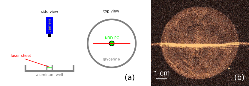
Figure 1: (a) Schematic of apparatus. (b) Sample image from experiments with initial conditions IC5, with both the height profile (bright line) and the fluorescence signal from the NBD-PC lipids (bright disk) at $t^{*}=21$ sec.

In order to verify the model prediction for the time-dependent distribution of surfactant concentration, we explore stricter tests of the model than have been performed previously. Using data from Fallest et al. Fallest-2010-FVS (for which $\Gamma$ is well above $\Gamma_{c}$), we make a detailed comparison between the model predictions and the measured surface height profiles $h(r,t)$ (from a laser line) and measured surfactant concentration profiles $\Gamma(r,t)$ (from azimuthal averages of fluorescent intensity at each point $\vec{r}$). Figure 1 provides a schematic of the apparatus and a sample image. The well-specified physical parameters additionally allow us to evaluate the accuracy of the characteristic timescale predicted for the spreading rate, rather than just the exponent. While we find approximate agreement in the spreading exponent and the coincidence of the surfactant leading edge with the capillary ridge, we also find two significant inconsistencies. First, there is a mismatch between the characteristic timescale between model and experiment. Second, the spatial distribution of the surfactant differs markedly from what is predicted in simulations. To account for the extent to which these discrepancies might be due to amounts of surfactant well beyond the monolayer regime, we perform new experiments, modified to allow for the detection of monolayer concentrations of surfactant ($\Gamma<\Gamma_{c}$). In these experiments, we observe a distribution of surfactant which differs from the model predictions. In addition, we find that there is no spreading capillary ridge, and that the spreading exponent for the leading edge of the surfactant is less than $1/10$. This value is well below predictions of the theory.

The outline of the paper is as follows. In §2, we provide details about the experimental setup and the materials used. In §3, we review the Gaver-Grotberg model [10], including a discussion of the choice of equation of state relating surfactant concentration to surface tension, and outline the finite difference method used for numerical simulation. In §4, we describe comparisons between numerical simulations and experimental results at initial concentrations well above $\Gamma_{c}$. As described above, we find partial agreement but also two inconsistencies when comparing experimental observations to numerical simulations. In an attempt to address the latter problem, in §5 we describe a hybrid model that takes the experimentally-measured $\Gamma(r,t)$ and uses that quantity (instead of the model for surfactant evolution) to generate the evolution of the surface height profile. We find that this provides reasonable agreement with the experimental data for $h(r,t)$. In particular, the timescale in the simulations is set by the experimental surfactant distribution, and the height profile dynamics therefore evolve according to the experimentally-observed timescale. In §6, we report new experiments with $\Gamma<\Gamma_{c}$ and find significant disagreement with the model predictions, as summarized above. We conclude in §7 with a discussion of the results and their significance.

2 Surfactant-Spreading Experiments

In our experiments, we simultaneously record the surface height profile $h(r,t)$ of the underlying glycerin fluid layer, as well as the local fluorescence intensity, which corresponds to the local concentration $\Gamma^{*}({\vec{r}},t)$ of insoluble lipids (surfactant) spreading on the surface. The basic apparatus, described in Fallest-2010-FVS and shown in Figure 1, consists of an aluminum well, a black light for exciting the NBD fluorophores, an oblique red laser line to illuminate the profile of the fluid surface, and a digital camera positioned directly above the experiment to capture the laser line and fluorescence; this apparatus is used for the data presented in §4. New experiments, presented in §6, are optimized to permit visualization of monolayer concentrations of surfactant. The bottom of the aluminum well is covered with a plasma-cleaned silicon wafer for improved reflectivity, and the fluorescent excitation is provided by 467 nm (blue) LEDs which coincide with the 464 nm absorption peak of the NBD fluorophore. A green laser line illuminates the profile of the fluid surface, so that both it and the fluorescently-emitted light pass through a band-pass filter centered at the emission peak (531 nm). These improvements to the optics permit us to collect images of the spreading dynamics at a framerate of 3 Hz and an integration time of $\frac{1}{4}$ second, using an Andor Luca R camera optimized for fluorescence measurements. The signal-to-noise ratio now sets a lower limit of ${\cal O}(10^{-2})\Gamma^{*}_{c}$ for the detection of surfactant.

For all experiments, we deposit 1-palmitoyl-2-{12-[(7-nitro-2-1, 3-benzoxadiazol-4-yl)amino]lauroyl} -sn-glycero-3-phosphocholine (abbreviated NBD-PC, from Avanti Polar Lipids) within a retaining ring which is lifted to begin the spreading process. This lipid molecule has one 12-carbon chain and one 16-carbon chain; the NBD fluorophore is attached to the 12-carbon chain. Experiments are conducted on a layer of 99.5% anhydrous glycerin, at an initial depth of $d=0.98\pm 0.03$ mm, and held at room temperature ($22.5\pm 1.5$ ^∘C). The lipids are initially deposited while dissolved in chloroform, which is allowed to evaporate for at least $30$ min before the retaining ring is lifted by a motor at $1$ mm/min. This allows sufficient time for the meniscus to drain before it detaches from the ring.

Symbol	Interpretation	Value
$\rho$	fluid density, glycerin	$1.26$ g/cm3
$\mu$	dynamic viscosity, glycerin	$0.83\pm.03$ Pa$\cdot$s [27]
$D_{s}$	surface diffusivity,surfactant	$10^{-4}$ cm2/sec [26]
$\sigma_{0}$	surface tension, clean glycerin	$63.4\pm 0.3$ dyne/cm [32]
$\sigma_{m}$	surfactant-contaminated surface tension	$35.3\pm 0.3$ dyne/cm [4]
$S$	change in surface tension, $S=\sigma_{0}-\sigma_{m}$	$28.1\pm.06$ dyne/cm
$\Gamma_{c}$	critical monolayer concentration	$0.3$ $\mu$g/cm2 [4]
$H_{0}$	initial fluid thickness	$0.98\pm.03$ mm
$R_{0}$	lateral dimension	$0.8$ cm or $1.4$ cm (ring radius)

Table 1: Key dimensional parameters.

	$M_{L}$ ($\mu$g)	$R_{0}$ (cm)	$\bar{\Gamma}_{0}^{*}$ $\mu$g/cm2)
IC1	0.85	$1.4$	$0.13$	$\bar{\Gamma}_{0}^{*}<\Gamma_{c}$
IC2	1.4	$1.4$	$0.22$
IC3	1.7	$1.4$	$0.26$
IC4	0.6	$0.8$	$0.30$
IC5	18.0	$1.4$	$2.73$	$\bar{\Gamma}_{0}^{*}>\Gamma_{c}$
IC6	18.0	$0.8$	$8.95$

Table 2: The six different initial conditions for the experiments presented in the paper.

The key material parameters for NBD-PC and glycerin are summarized in Table 1. The initial conditions (IC) for the experiment are distinguished by the initial concentration $\bar{\Gamma}_{0}^{*}$ of surfactant deposited within the ring, defined by

$$\bar{\Gamma}^{*}_{0}\equiv\frac{M_{L}}{\pi R_{0}^{2}},$$ (1)

where $M_{L}$ is the mass of NBD-PC deposited and $R_{0}$ is the radius of the ring. Although a small amount of surfactant remains on the ring after it has been lifted, we nonetheless use the nominal concentration $\bar{\Gamma}_{0}^{*}$ to describe the different initial conditions in Table 2. The experiments presented in §4 all begin from IC6, with $\bar{\Gamma}_{0}^{*}$ above the critical monolayer concentration $\Gamma_{c}$. The experiments of §6 employ initial conditions that probe the monolayer regime (below $\Gamma_{c}$).

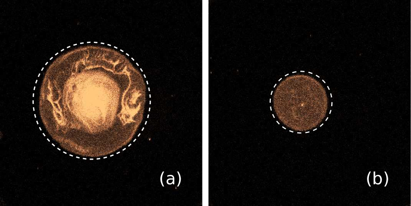
Figure 2: Fluorescence intensity (proxy for surfactant concentration) measured at $t^{*}=5$ sec, for experiments with initial conditions (a) IC6 and (b) IC4. The dashed circles (of radii 3.4 cm and 1.1 cm, respectively), highlight the corrugations in the leading edge.

Figure 1b shows a sample image of both the laser line (measures the height profile $h^{*}(r)$ and the location $r_{M}$ of its maximum), and the fluorescence intensity (measures the surfactant distribution $\Gamma^{*}(r)$ after azimuthal averaging and the location $r_{0}$ of its leading edge). Figure 2 shows sample images of the surfactant distribution alone, for a representative $\bar{\Gamma}^{*}_{0}>\Gamma_{c}$ case and a $\bar{\Gamma}^{*}_{0}<\Gamma_{c}$ case. In each image, a sharp interface between the surfactant-covered and bare glycerin is readily visible; the location $r_{0}$ of this interface is determined by identifying the annulus of maximum fluorescence intensity gradient. While the surfactant distribution is uniform for $\bar{\Gamma}_{0}^{*}<\Gamma_{c}$, several heterogeneities are present when $\bar{\Gamma}_{0}^{*}>\Gamma_{c}$. First, the central region contains a greater concentration of surfactant than the regions closer to the leading edge, an effect that we will explore in more detail below. Second, there are filamentary patches of high concentration which also propagate out from the central region, becoming more dilute during the spreading dynamics. We also note that the outer edge of surfactant in both cases has corrugations; in the figure, white circles are imposed to emphasize that the edges are not quite circular. Although the surfactant distributions are never precisely axisymmetric, we nonetheless record the distribution by averaging azimuthally. Moreover, in the model and simulations of the following sections, we assume that the surfactant distributions are axisymmetric.

3 Model

We consider the model derived by Gaver and Grotberg Gaver-1990-DLS for a single layer of surfactant molecules spreading on a thin liquid film. The model is a coupled system of partial differential equations for the height $h(r,t)$ of the fluid free surface and the concentration $\Gamma(r,t)$ (mass per unit area) of surfactant. We assume axisymmetric spreading, and the variables are nondimensionalized: $r=\frac{1}{R_{0}}r^{*}$, $t=\frac{1}{T}t^{*}$, $h=\frac{1}{H_{0}}h^{*}$, $\Gamma=\frac{1}{\Gamma_{c}}\Gamma^{*}$, where ^∗ indicates the dimensional variable.

$$h_{t}+\frac{1}{r}\left({\textstyle{1\over 2}}rh^{2}\sigma(\Gamma)_{r}\right)_{r}=\beta\frac{1}{r}\left({\textstyle{1\over 3}}rh^{3}h_{r}\right)_{r} - \kappa\frac{1}{r}\left({\textstyle{1\over 3}}rh^{3}\left(h_{rr}+\frac{1}{r}h_{r}\right)_{r}\right)_{r}$$ (2a)

$$\Gamma_{t}+\frac{1}{r}\left(rh\Gamma\sigma(\Gamma)_{r}\right)_{r}=\beta\frac{1}{r}\left({\textstyle{1\over 2}}rh^{2}\Gamma h_{r}\right)_{r} - \kappa\frac{1}{r}\left({\textstyle{1\over 2}}rh^{2}\Gamma\left(h_{rr}+\frac{1}{r}h_{r}\right)_{r}\right)_{r}$$ (2b)

$$+ \delta\frac{1}{r}\left(r\Gamma_{r}\right)_{r}.$$

The nondimensional parameter groups $\beta$, $\kappa$, and $\delta$ result from nondimensionalization, using values of physical parameters listed in Table 1. The parameter $\beta=\frac{\rho gH_{0}^{2}}{S}\approx 0.42$ balances gravity and Marangoni forces, $\kappa=\frac{\sigma_{m}H_{0}^{2}}{SR_{0}^{2}}\approx 0.019$ is the ratio of the capillary driving forces to the forces from the surface tension gradient, and $\delta=\frac{1}{Pe}=\frac{\mu D}{SH_{0}}\approx 3.0\times 10^{-5}$ represents the surface diffusion of the surfactant molecules where $Pe$ is the Péclet number. The function $\sigma(\Gamma)$ expresses the dependence of surface tension $\sigma$ on surfactant concentration $\Gamma$. It is specified by an equation of state, as discussed in the next subsection. The timescale $T=\frac{\mu R_{0}^{2}}{SH_{0}}\approx 2.0$ sec achieves a balance between the terms on the left side of (2). In §4.1, we test this predicted timescale directly.

With $\delta>0$, the leading edge of the surfactant distribution is not precisely defined, since $\Gamma(r,t)>0$ for all $r$ and for all $t>0$. Nonetheless, although $\delta$ is very small, it is retained in numerical simulations, apart from one case, in which $\delta$ is set to zero in order to track the leading edge of the surfactant distribution.

Since the boundary at $r=0$ is not a physical boundary, boundary conditions there are natural; for large $r$, the free surface is undisturbed on the time scale of the experiment, and the surfactant concentration is expected to be identically zero:

$$h_{r}(0,t)=\Gamma_{r}(0,t)=0,\qquad h_{rrr}(0,t)=0,$$

$$\lim_{r\to\infty}h(r,t)=1,\qquad\lim_{r\to\infty}\Gamma(r,t)=0.$$ (3)

A finite difference method is used to simulate (2) and is summarized in the Appendix. The initial condition $h(r,0)$ is chosen to reflect the initial height profile in the experiment, as the fluid meniscus detaches from the ring, thereby releasing the surfactant to spread across the fluid surface. The initial distribution $\Gamma_{0}(r)$ of surfactant within the ring is unknown, and is varied in the simulations to test its effect on the spreading.

$$h(r,0) = \begin{cases}a\sin\left(2r-\frac{\pi}{3}\right)+(1+a),&\mbox{0}\leq r<\frac{11\pi}{12}\\[6.0pt] 1,&\frac{11\pi}{12}<r<R_{max},\end{cases}$$

$$\Gamma(r,0) = \begin{cases}\Gamma_{0}(r),&\mbox{0}\leq r<\frac{5\pi}{12}\\[6.0pt] 0,&\frac{5\pi}{12}<r<R_{max}.\end{cases}$$ (4)

In the simulations, we set $a=0.15$ in order provide a match between the initial condition and the measured height profiles at later times. For the simulations, the location $R_{max}$ of the edge of the domain is taken large enough that the influence of the boundary conditions at $r=R_{max}$ is negligible over the time of the experiment. We take $R_{max}=10$, but display graphs of $h$ and $\Gamma$ over the smaller domain, $0\leq r\leq 7$.

3.1 Equation of State

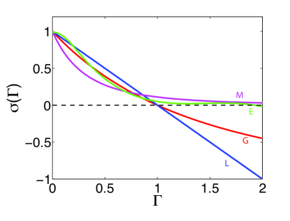
Figure 3: The four equations of state used in the model, L: linear (5), G: Langmuir (7), E: measured (6), M: multilayer (8).

In order to compare the model (2) to the results of the experiments described in Fallest-2010-FVS, we need to choose an appropriate equation of state relating the surfactant concentration $\Gamma$ to the surface tension $\sigma$. However, the model is valid only for a single layer of surfactant molecules ($\Gamma\leq 1$) but the experiments are conducted with initial surfactant concentrations up to $\Gamma=30$. In an attempt to extend the model to the regime of the experiment, we consider different equations of state $\sigma=\sigma(\Gamma)$ that have been proposed in the literature. In Figure 3, we show the graphs of four such functions; we argue below that only the graph labeled M is suitable for modeling the full range of surfactant concentrations we wish to consider.

The equation of state we seek should have the following properties: $\sigma^{\prime}(\Gamma)<0$, expressing the effect that increasing surfactant concentration decreases surface tension; $0<\sigma(\Gamma)\leq 1$, since this is the range of values of surface tension in our nondimensionalization, with $\sigma(0)=1$. As can be seen in the figure, only graph M has these properties.

The linear equation of state

$$\sigma(\Gamma)=1-m\Gamma$$ (5)

and has been used widely [20, 23, 6, 22]. This equation is generally chosen for simplicity; it is also a reasonable linear approximation to nonlinear equations of state at low concentration. Note that $\frac{d\sigma(\Gamma)}{d\Gamma}=-m$ is a negative constant ($m=1$ in the figure). In the case of more than a monolayer of surfactant, this equation suggests that the surface tension decreases endlessly which is not physical, as surfactant concentration beyond a monolayer has little further effect in decreasing surface tension.

Bull et al. Bull-1999-SSS determined an equation of state for NBD-PC on glycerin by fitting the data obtained using a tensiometer. Using the nondimensional parameters in Table 1 ($\Gamma_{c}\approx 0.3$ $\mu$g/cm²), the corresponding formula for $\sigma(\Gamma)$ is

$$\sigma(\Gamma)=\begin{cases}0.28\cos\left(6.28\Gamma\right)+0.71,&\Gamma<0.25\\ 1.26-2.6\Gamma+1.8\Gamma^{2}-0.41\Gamma^{3},&0.25\leq\Gamma\leq 1.67.\end{cases}$$ (6)

However, this formula is applicable only for surfactant concentrations below approximately $2\Gamma_{c}$ ($\Gamma<2$ in Figure 3), as $\sigma^{\prime}(\Gamma)$ decreases sharply for larger values of $\Gamma$.

The Langmuir equation of state, used in Gaver-1990-DLS and Warner:2004, is

$$\sigma(\Gamma)=\frac{\eta+1}{(1+\Theta(\eta)\Gamma)^{3}}-\eta$$ (7)

where $\Theta(\eta)=\left(\frac{\eta+1}{\eta}\right)^{\frac{1}{3}}-1$ and $\eta=\frac{\sigma_{m}}{S}$. When only a small amount of surfactant is introduced, a large change in the surface tension occurs and as the surfactant comes close to saturation (a monolayer) then adding more surfactant does not alter the surface tension very much. However, the range of $\sigma(\Gamma)$ is $[-\eta,1]$ rather than $[0,1]$. The multiple layer equation of state used by Borgas and Grotberg Borgas-1988-MFT is related to the Langmuir equation of state:

$$\sigma(\Gamma)=(1+\eta\Gamma)^{-3}$$ (8)

This formulation is based on properties of surface tension discussed by Sheludko Sheludko:1966 and by an experimental fit by Foda and Cox Foda-1980 who worked with an oil layer on water. In addition, $\sigma(\Gamma)$ remains positive at large $\Gamma$, allowing us to simulate much higher concentrations of surfactant. Therefore, we use Eq. (8) for the simulations.

4 High Surfactant Concentration ($\bar{\Gamma}_{0}^{*}>\Gamma_{c}$)

The $r_{0}(t)\propto t^{1/4}$ spreading behavior predicted by (2) has already been observed in prior experiments with oleic acid on a water-glycerin mixture [5] and NBD-PC on glycerin [8]. In this section, we make a more detailed comparison between the results from experiments and numerical simulations, using data from Fallest et al. Fallest-2010-FVS. While we are able to obtain reasonable agreement in the height profile shapes, a comparison of the dynamics (§4.1) requires that we adjust the timescale. In §4.2, we show a significant discrepancy between the observed distribution of surfactant and the prediction from simulations, even though the location and time evolution of the leading edge of the surfactant layer agree well, as detailed in §4.3. We also describe attempts to capture the experimentally observed surfactant distribution by varying the initial distribution $\Gamma_{0}(r)$ in the simulations.

4.1 Timescale

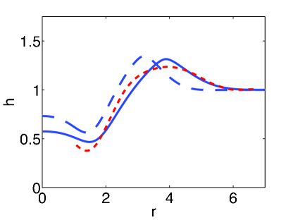
Figure 4: Surface height profiles $h(r)$ measured at $t^{*}=5$ sec in the experiment (short dashed lines, red), compared to numerical solutions at nondimensional times. Long dashed lines: $t=2.5$ (uses calculated $T=2.0$ sec); Solid line: $t=5$ (uses better-fitting $T=1.0$ sec). Data are from Fallest et al. Fallest-2010-FVS, with initial condition IC6.

In order to compare the model and experiment, we convert the simulation results from dimensionless time $t$ to dimensional time $t^{*}$ using the relation $t=\frac{t^{*}}{T}$, where $T\equiv\frac{\mu R_{0}^{2}}{SH_{0}}\approx 2.0$ sec is calculated from the dimensional parameters listed in Table 1. Previous simulations [11, 5] have treated the lengthscale $R_{0}$ as a free parameter, effectively adjusting the timescale to agree with the experimental observations. However, for the experiments analyzed here, the ring radius $R_{0}=0.8$ cm is known and consequently the time scale $T$ is determined, with no free parameters.

In Figure 4, we observe that the simulated height profile and the experimental data are inconsistent at $t^{*}=5$ sec if the determined value $T=2.0$ sec is used: neither the peak location nor its width are in agreement with the model. However, if we use $T=1.0$ sec instead of $T=2.0$ sec, thereby comparing the simulation at the later time $t=5$ to the same experimental data at $t^{*}=5$ sec, then both the position and width of the ridge are in approximate agreement between the model and experiment. This agreement between simulation and experiment using the timescale $T=1.0$ sec is observed to hold for all times beyond an initial transient. Although an explanation for the discrepancy between times scales awaits further investigation, we use the empirically-determined $T=1.0$ sec as the timescale for the remaining comparisons in the paper.

4.2 Height Profile and Surfactant Distribution

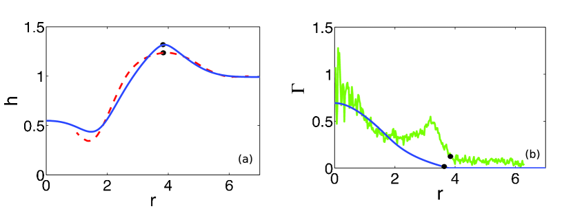
Figure 5: (a) Surface height profiles $h(r)$ measured at $t^{*}=5$ seconds in the experiment (dashed lines) and $t=5$ in numerical solution (solid line); the location $r=r_{M}$ of the peak is marked with a $\bullet$. (b) The corresponding surfactant concentration profiles $\Gamma(r)$ in the experiment (noisy) and numerical solution (smooth); the location $r=r_{0}$ of the leading edge of the surfactant is marked with a $\bullet$. Data are from Fallest et al. 2010, with initial condition IC6.

In Figure 5 we compare the simulated and measured surface profiles and surfactant distributions, using the model parameters described in §4.1 and experimental data from Fallest et al. Fallest-2010-FVS. As can be seen in Figure 5, the height profiles $h(r,5)$ are in approximate agreement: locations of the maximum and minimum are in approximate agreement between simulation and experiment, and the overall shapes are similar. In contrast, the measured surfactant distribution has quite a different shape from the distribution predicted by the simulations. While the model predicts a smooth decrease in $\Gamma(r,5)$ away from the central peak, experiments instead show an extended plateau over which the surfactant concentration is nearly constant, and which appears to be drawn out of a reservoir, near the peak concentration at $r=0$. For longer times, the plateau extends and decreases in height. These features do not appear in the numerical simulations.

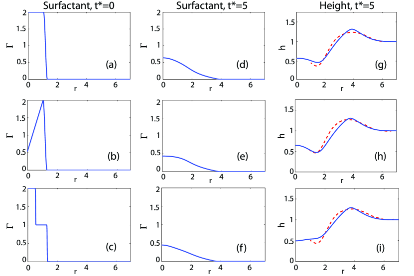
Figure 6: (a-c) Three different surfactant initial conditions, with the resulting (d-f) surfactant concentration profiles $\Gamma(r)$ and (g-i) surface height profiles $h(r)$ from numerical solutions at $t=5$. The experimental height profiles at $t^{*}=5$ seconds are the same in each case, and are shown as dashed lines.

In the experiment, the total surfactant mass is known, but its initial spatial distribution within the retaining ring is not measured. Consequently, there is some uncertainty about the appropriate initial condition $\Gamma(r,0)=\Gamma_{0}(r)$. We explore whether the choice of $\Gamma_{0}(r)$ could change the simulations enough to replicate the expanding plateau in the experimentally observed surfactant distributions. We tested three different functions $\Gamma_{0}$, shown in Figure 6: (a) Uniform distribution; (b) Surfactant more concentrated near the retaining ring; (c) Step distribution. The initial free surface height profile $h(r,0)$ is the same in each case, given by (3).

The results of these simulations at time $t^{*}=5$ sec (after short-time transients have died out) are shown in Figure 6. In the middle column, we observe that the distribution $\Gamma$ of surfactant does not exhibit a plateau for any of the initial conditions, while in the final column we see that the height profiles show broad agreement with the experiment in each case.

4.3 Spreading Exponent

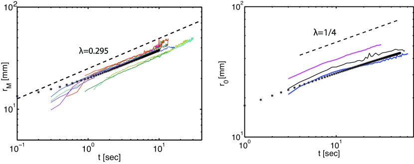
Figure 7: Comparison between spreading rates of (a) the location of the maximum of the surface height profile $h(r)$ and (b) the location of the leading edge of surfactant in both experiment and simulation. Colored lines are from experiments with IC6 adapted from Fallest et al. 2010, black dots are from simulations. Dashed lines are (a) comparison to best-fit $t^{\alpha}$ with $\alpha=0.295$ and (b) comparison to $t^{1/4}$.

In spite of the disagreements above, we observe that the spreading dynamics of the model and experiment are in good agreement when the artificial choice of $T=1$ sec is used. The surface diffusion term $\delta\Gamma_{xx}$ in (2a) smooths the surfactant profile, and guarantees $\Gamma(r,t)>0$ for all $r\geq 0$ and $t>0$. This means the surfactant distribution has no clearly defined leading edge. Since $\delta\approx 10^{-5}$ has a very small effect, we take $\delta=0$ in these simulations. The surfactant distribution is then supported at each $t>0$ on a bounded interval $0\leq r\leq r_{0}(t)$, and the leading edge $r=r_{0}(t)$ can be tracked using the numerical scheme described in Peterson-2012-SSS with $\beta\kappa>0$. In Figure 7(b), $r_{0}(t)$ is shown as a dotted line; on the log-log plot the numerical solution is compared to the experimental results and to the analytic form $r_{0}(t)\sim t^{1/4}$ derived from the similarity solution of Jensen-1992-ISS, in which $\beta=\kappa=\delta=0$.

We also tracked the capillary ridge $r=r_{M}(t)$, where the height profile $h(r,t)$ has a maximum. In Figure 7(a) we show the numerical solution as a dotted line, and compare to experimental results, with an approximate slope shown with a dashed line. The data for the leading edge of the surfactant agrees with the $t^{\frac{1}{4}}$ prediction of the model. The capillary ridge moves faster as it catches up to the surfactant leading edge; it is best fit by $t^{0.295}$ over the duration of the experiment.

Note that for $\beta=\kappa=\delta=0$ in the model, the fluid surface experiences a discontinuity at the leading edge $r=r_{0}(t)$ of the surfactant, and the fluid is undisturbed ahead of this front. It is worth noting that with $\delta=0$, the surfactant distribution still has a finite extent when $\beta$ or $\kappa$ is non-zero, but the disturbance of the film does not. In fact, the surface tension gradient induced at the leading edge $r=r_{0}(t)$ of the surfactant generates fluid motion ahead of $r_{0}$.

5 Hybrid Model

Due to the failure of the model equations (2) to capture the spatial distribution of the surfactant, as discussed in §4, we consider whether there is a fundamental modeling problem with the equation (2b) for the evolution of $\Gamma(r,t)$. Given that the height profile $h(r,t)$ evolves in a quantitatively reasonable way, we leave (2a) intact, but take $\Gamma(r,t)$ from the experiment and use it to determine $h(r,t)$ numerically.

The experimental data for $\Gamma$ are noisy, and occur at discrete times; we must smooth and interpolate the data for use in the numerical scheme to determine $h$. The first step is to smooth the experimental data at each recording time. This is achieved using the MATLAB smooth function, which performs a moving spatial averages over a specified span of data points; we found a low-pass filter with a span of 21 points to be effective.

The experimental data are recorded at one second intervals; however, the numerical method requires the time step $\Delta t$ to be on the order of ${\cal O}(10^{-3})$ for stability. To remedy this inconsistency, we interpolate the smoothed surfactant profiles to obtain functions that can be used to represent the surfactant concentration $\Gamma(r,t)$ at all values of $r$ and $t$.

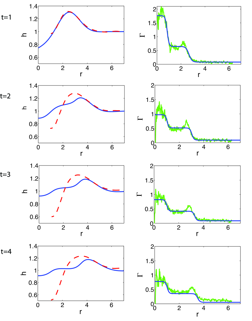
Figure 8: (a-d) Comparison of the surface height profiles $h(r)$ from the numerical simulations (solid blue) and experimental data (dashed red). (e-h) The corresponding surfactant profiles from the experiment, smoothed data (smooth blue) and raw data (noisy green). The profiles are shown at $t^{*}=1,2,3,4$ sec.

First, we use the nonlinear fit function, nlinfit in MATLAB to fit the smoothed surfactant data at each experimental recording time to a function with a graph consistent with the two step structure of the experimental surfactant distributions. As observed in Figure 8, the experimental surfactant distribution $\Gamma$ is roughly constant in each of the two steps. With this in mind, we use the function

$$\Gamma(r,j)=a_{1}^{j}-a_{2}^{j}\tanh\left(\frac{r-a_{3}^{j}}{a_{4}^{j}}\right)-a_{5}^{j}\tanh\left(\frac{r-a_{6}^{j}}{a_{7}^{j}}\right)$$ (9)

to fit the surfactant profile at each time $t^{*}$ for which we have data, where $t^{*}=j,j=1,2,\dots,10$ sec. This procedure generates coefficients $a_{1}^{j},\dots,a_{7}^{j}$.

Next we create polynomial functions, $a_{i}^{*}(t^{*}),i=1\dots 7$ from the discrete values $a_{i}^{j},j=1,\dots 10$ using polyfit in MATLAB, but with a restriction that the mass of the surfactant must be conserved. Since the numerical code requires nondimensional time $t=0.5t^{*}$, we define $a_{i}(t)=a_{i}^{*}(2t),i=1\dots 7$. These functions define the surfactant concentration profiles that approximate the experimental data:

$$\Gamma(r,t)=a_{1}(t)-a_{2}(t)\tanh\left(\frac{r-a_{3}(t)}{a_{4}(t)}\right)-a_{5}(t)\tanh\left(\frac{r-a_{6}(t)}{a_{7}(t)}\right).$$ (10)

We update the height profile using the finite difference scheme used in §4 with boundary conditions (3) and the surfactant concentration profile using (10):

$$h_{j}^{n+1}=h_{j}^{n} + \Delta t\frac{1}{r_{j}\Delta r}\left(\mathcal{F}_{j+{\textstyle{1\over 2}}}^{n+1}-\mathcal{F}_{j-{\textstyle{1\over 2}}}^{n+1}\right)$$ (11a)

$$\Gamma_{j}^{n+1}=a_{1}(t^{n+1}) - a_{2}(t^{n+1})\tanh\left(\frac{r-a_{3}(t^{n+1})}{a_{4}(t^{n+1})}\right)$$ (11b)

$$- a_{5}(t^{n+1})\tanh\left(\frac{r-a_{6}(t^{n+1})}{a_{7}(t^{n+1})}\right).$$

The flux functions $F_{j}^{n}$ are described in the appendix.

In Figure 8, we show simulation results using initial condition (3) and parameters $\beta=0.5,\;\kappa=0.5$. Note that this value of $\kappa$ is larger than the value suggested by the nondimensional grouping. This is in order to smooth the height profile, which otherwise would develop multiple persistent ridges, due to the steep gradient in the surfactant concentration. Multiple ridges are observed at very early time in the simulations discussed in § 4.2 but then the gradient in the surfactant is quickly smoothed. In this case, the ridge in the height profile from the surfactant gradient and the one from the initial condition (due to the lifting of the ring) combine at very early time and then propagate as one. By contrast, in the experiment the surfactant distribution does not experience this smoothing and consequently when the experimental values for the surfactant concentration are input into the height equation a second ridge develops and persists. By increasing the capillarity parameter $\kappa$, the height profile is smoothed, and the numerical height profile becomes more similar to the experimental height profile.

The surface height profile simulated using this hybrid model exhibits an evolution and shape that is comparable to the experiment. We conclude that the equation modeling surfactant molecule motion through passive transport by the surface fluid is fundamentally flawed, and is missing some physical or chemical properties that would generate the surfactant distributions observed in the experiment.

6 Monolayer Surfactant Concentration ($\bar{\Gamma}_{0}^{*}<\Gamma_{c}$)

Because the original model (2) was developed for use with monolayer concentrations of surfactants ($\bar{\Gamma}_{0}^{*}<\Gamma_{c}$), we conduct new experiments in this regime. In addition, these experiments help elucidate the discrepancies between model and experiment at the higher concentrations. Performing experiments at lower surfactant concentrations requires improvements of our earlier techniques (see §2) in order to visualize lower surfactant concentrations. We perform experiments starting from four different initial concentrations, IC1-IC4 in Table 2, all of which result in similar spreading dynamics, described below. In no case do we find that the agreement with the model is improved over the $\bar{\Gamma}_{0}^{*}>\Gamma_{c}$ case: height profiles, surfactant distribution, and the spreading dynamics all significantly disagree with the model predictions.

6.1 Height Profile and Surfactant Distribution

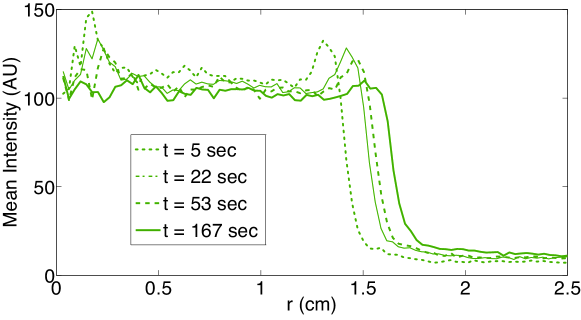
Figure 9: Azimuthally-averaged fluorescence intensity at a distance $r$ from the center of the surfactant region, shown at representative times, taken from an experiment with IC4 ($\bar{\Gamma}_{0}^{*}<\Gamma_{c}$).

As illustrated in Figure 2, and shown quantitatively in Figure 9, the spreading region has an approximately uniform surfactant distribution throughout the lipid-covered area. The leading edge, located at $r_{0}$, exhibits a sharp interface (approximately $0.5$ mm wide, neglecting azimuthal corrugations) that does not broaden as the surfactant spreads outward. Instead, the overall concentration decreases throughout the lipid-covered region. These observations are in disagreement with the model, which predicts a monotonically decreasing profile (see Figure 5) with a gradual and broadening transition to $\Gamma=0$ at $r_{0}$.

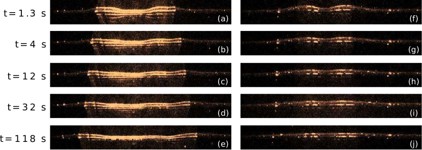
Figure 10: Images comparing the laser profile for two experiments with IC5 (a-e) ($\bar{\Gamma}_{0}^{*}>\Gamma_{c}$) and IC2 (f-j) ($\bar{\Gamma}_{0}^{*}<\Gamma_{c}$) at five different times. The uppermost bright line in each image is the reflection from the air glycerin interface, and is used to measure the free surface height profile $h(t)$.

Figure 10 provides a comparison between the behavior of the fluid ridge in two regimes. For $\bar{\Gamma}_{0}^{*}>\Gamma_{c}$, the glycerin is pushed out by the surface tension gradient, and forms a capillary ridge at the surfactant edge (panels f-j). As already discussed in §4.2, these two features travel outward together. This is consistent with simulations at high or low surfactant concentrations, that show a fluid ridge propagating outwards due to Marangoni forces. In contrast, the experimental data in the $\bar{\Gamma}_{0}^{*}<\Gamma_{c}$ regime (panels a-e) show an initial ridge (due to the meniscus at the ring) collapsing rapidly in place, and no discernible ridge propagating outwards.

6.2 Spreading Exponent

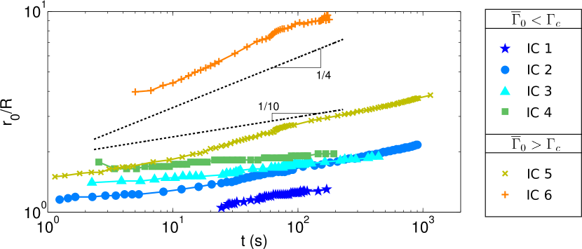
Figure 11: The spreading dynamics of the location of the leading edge of the fluorescence intensity ($r_{0}$), scaled by the ring radius $R_{0}$. The dashed lines corresponding to $t^{1/4}$ and $t^{1/10}$ spreading behavior are shown for comparison.

Given the significant differences between the observed and modeled $h(r,t)$ and $\Gamma(r,t)$, it is unsurprising that we observe the spreading dynamics to be quite different as well. In Figure 11, we plot the position of the leading edge $r_{0}$ as a function of time, for experiments in both the monolayer regime of IC1-IC4 and for higher initial concentrations (IC5-IC6). For $\bar{\Gamma}_{0}^{*}<\Gamma_{c}$ (IC1-IC4) the dynamics all follow a form $r_{0}\propto t^{\alpha}$, with $\alpha\lesssim 1/10$. Remarkably, this is reminiscent of Tanner’s law for fluid spreading on a solid [30]. For slightly larger values of $\bar{\Gamma}_{0}^{*}$ (IC5), we observe faster surfactant spreading dynamics initially, but $r_{0}\propto t^{\alpha}$ with $\alpha\approx 1/10$ at later times. This slow-spreading regime was not reached in the runs with much larger values of $\bar{\Gamma}_{0}^{*}$ (IC6), for which $\alpha$ remains close to $\alpha=1/4$, as predicted in [19]. The decrease in $\alpha$ for low surfactant concentrations suggests a transition in the dynamics which is not covered by the model equations. The differing prefactors for the various runs is probably a result of variations in $\bar{\Gamma}_{0}^{*}$ due to some lipid molecules remaining on the ring after it lifts off, an effect that is more significant at lower concentrations.

7 Discussion

Current mathematical models that describe the dynamics of the free surface of a thin fluid layer subject to forces induced by variations in surface tension contain two key assumptions: (1) lubrication theory is valid, and (2) surfactant molecules are primarily passively-transported by the fluid motion along the surface, along with negligible molecular diffusion. However, the dependence of surface forces on local variations in surfactant concentration is not completely settled, especially for larger concentrations. Due to the coupling between the motion of the underlying fluid and the spreading of surfactant molecules, it is crucial to compare results from simulations and experiments for both fluid motion (through surface deformations) and the dynamics of surfactant distribution.

In this paper, we compare model predictions to experiments that include the simultaneous visualization of the fluid height profile and the distribution of surfactant, both above and below the critical monolayer concentration $\Gamma_{c}$. In both cases, we find serious inconsistencies between the model and the experiments. The aspect ratio for the experiments is $\frac{H_{0}}{R_{0}}\approx 0.1$, which justifies the use of the lubrication approximation; we have not verified the magnitude of the vertical velocity profile. At all initial concentrations, both above and below $\Gamma_{c}$, the spatial distribution of surfactants does not follow the smooth, monotonically-decreasing profiles predicted by the model. At low surfactant concentrations ($\bar{\Gamma}_{0}^{*}<\Gamma_{c}$, for which the models were originally developed), the distribution is highly-uniform with a sharp interface at the leading edge. Second, spreading occurs much more slowly than is predicted by the model. For all experiments with $\bar{\Gamma}_{0}^{*}<\Gamma_{c}$, the spreading dynamics of the leading edge approximately follow a power law $r_{0}(t)\propto t^{\alpha}$, with $\alpha\lesssim 1/10$. This is significantly smaller than the $\alpha=1/4$ predicted by the natural scaling in the model. Interestingly, this exponent is also markedly different from the exponent of $1/2$ to $3/4$ observed by Gaver and Grotberg Gaver-1992-DST for oleic acid and by Bull et al. [4] for NBD-PC. In the former case, the measurement technique relies on the model for interpretation of experimental results, while in the later the $2$ mm fluid layer thickness may be large enough that deviations from the lubrication approximation are significant. For $\bar{\Gamma}_{0}^{*}>\Gamma_{c}$, even though $\alpha\approx 1/4$, there is a mismatch by a factor of two between the timescales predicted in the model and observed in experiment. These inconsistencies are not resolved by changing assumptions concerning the initial distribution of surfactant. Moreover, if a measured $\Gamma(r,t)$ is incorporated directly into the lubrication model, then the timescale issue is no longer present, as the spreading ridge is simply driven by the spreading surfactant.

One untested assumption is the functional form of the equations of state which have been considered to date. The lack of spreading ($\alpha\lesssim 1/10$ for very low concentrations) might indicate that the assumed $\sigma(\Gamma)$ equation of state is inadequate. If there were a value of $\Gamma$ below which there were no longer a significant surface tension gradient, a lack of spreading would be expected. In fact, in static surface-pressure measurements of diolein, oleyl alcohol, and lecithin on water, such an effect has been observed [17]. Future work to make similar measurements for NBC-PC, potentially locating a second transition point, may clarify the reason for the reduction in spreading. Another possibility is that the passive transport model for surfactant distribution on the free surface is missing one or more effects that influence on the dynamics of insoluble surfactant spreading on thin liquid films.

8 Acknowledgments

We are grateful for support from the National Science Foundation under grant number DMS-0968258 and Research Corporation under grant number 19788. In addition, we wish to thank Rachel Levy for valuable conversations concerning surfactant spreading.

Appendix

We summarize the finite difference method used to generate numerical results for system (2). Simulations are conducted on a large interval $0\leq r\leq R$. For simplicity, we consider uniformly distributed grid points $r_{j}=j\Delta r,j=1,\dots,N$, where $\Delta r=R/N$. At each time $t_{n}=n\Delta t,\ n\geq 0$, let $h_{j}^{n}\approx h(r_{j},n\Delta t)$ and $\Gamma_{j}^{n}\approx\Gamma(r_{j},n\Delta t)$. We use the standard notation for spatial averages of $u_{j}^{n}=u(r_{j},t_{n})$,

$$\bar{u}^{n}_{j+{\textstyle{1\over 2}}}\equiv\frac{u_{j+1}^{n}+u_{j}^{n}}{2}.$$ (12)

The numerical method is an implicit finite difference scheme in conservative form:

$$h_{j}^{n+1} = h_{j}^{n}+\Delta t\frac{1}{r_{j}\Delta r}\left(\mathcal{F}^{n+1}_{j+{\textstyle{1\over 2}}}-\mathcal{F}^{n+1}_{j-{\textstyle{1\over 2}}}\right)$$ (13a)

$$\Gamma_{j}^{n+1} = \Gamma_{j}^{n}+\Delta t\frac{1}{r_{j}\Delta r}\left(\mathcal{G}^{n+1}_{j+{\textstyle{1\over 2}}}-\mathcal{G}^{n+1}_{j-{\textstyle{1\over 2}}}\right).$$ (13b)

The fluxes inherit the structure of the PDE system (2) (note that we have dropped the $n+1$ superscript)

$$\mathcal{F}_{j+{\textstyle{1\over 2}}} = {\textstyle{1\over 2}}\mathcal{F}_{j+{\textstyle{1\over 2}}}^{1}+{\textstyle{1\over 3}}\beta\mathcal{F}_{j+{\textstyle{1\over 2}}}^{2}+{\textstyle{1\over 3}}\kappa\mathcal{F}_{j+{\textstyle{1\over 2}}}^{3}$$ (14a)

$$\mathcal{G}_{j+{\textstyle{1\over 2}}} = \mathcal{G}_{j+{\textstyle{1\over 2}}}^{1}+{\textstyle{1\over 2}}\beta\mathcal{G}_{j+{\textstyle{1\over 2}}}^{2}+{\textstyle{1\over 2}}\kappa\mathcal{G}_{j+{\textstyle{1\over 2}}}^{3}+\delta\mathcal{G}_{j+{\textstyle{1\over 2}}}^{4}.$$ (14b)

The individual fluxes are expressed as

$$\mathcal{F}_{j+{\textstyle{1\over 2}}}^{1} = \bar{r}_{j+{\textstyle{1\over 2}}}\left(\bar{h}_{j+{\textstyle{1\over 2}}}\right)^{2}\sigma^{\prime}\left(\bar{\Gamma}_{j+{\textstyle{1\over 2}}}\right)\frac{\Gamma_{j+1}-\Gamma_{j}}{\Delta r}$$ (15a)

$$\mathcal{F}_{j+{\textstyle{1\over 2}}}^{2} = \bar{r}_{j+{\textstyle{1\over 2}}}\left(\bar{h}_{j+{\textstyle{1\over 2}}}\right)^{3}\frac{h_{j+1}-h_{j}}{\Delta r}$$ (15b)

$$\mathcal{F}_{j+{\textstyle{1\over 2}}}^{3} = \bar{r}_{j+{\textstyle{1\over 2}}}\left(\bar{h}_{j+{\textstyle{1\over 2}}}\right)^{3}\frac{\mathcal{E}_{j+2}-\mathcal{E}_{j}}{2\Delta r}$$ (15c)

$$\mathcal{E}_{j+2} = \frac{h_{j+3}-2h_{j+2}+h_{j+1}}{\Delta r^{2}}+\frac{1}{\bar{r}_{j+\frac{3}{2}}}\frac{h_{j+2}-h_{j+1}}{\Delta r}$$ (15d)

$$\mathcal{G}_{j+{\textstyle{1\over 2}}}^{1} = \bar{r}_{j+{\textstyle{1\over 2}}}\bar{h}_{j+{\textstyle{1\over 2}}}\bar{\Gamma}_{j+{\textstyle{1\over 2}}}\sigma^{\prime}\left(\bar{\Gamma}_{j+{\textstyle{1\over 2}}}\right)\frac{\Gamma_{j+1}-\Gamma_{j}}{\Delta r}$$ (15e)

$$\mathcal{G}_{j+{\textstyle{1\over 2}}}^{2} = \bar{r}_{j+{\textstyle{1\over 2}}}\left(\bar{h}_{j+{\textstyle{1\over 2}}}\right)^{2}\bar{\Gamma}_{j+{\textstyle{1\over 2}}}\frac{h_{j+1}-h_{j}}{\Delta r}$$ (15f)

$$\mathcal{G}_{j+{\textstyle{1\over 2}}}^{3} = \bar{r}_{j+{\textstyle{1\over 2}}}\left(\bar{h}_{j+{\textstyle{1\over 2}}}\right)^{2}\bar{\Gamma}_{j+{\textstyle{1\over 2}}}\frac{\mathcal{E}_{j+2}-\mathcal{E}_{j}}{2\Delta r}$$ (15g)

$$\mathcal{G}_{j+{\textstyle{1\over 2}}}^{4} = \bar{r}_{j+{\textstyle{1\over 2}}}\frac{\Gamma_{j+1}-\Gamma_{j}}{\Delta r}.$$ (15h)

In the hybrid model of §5, the values of $\Gamma_{j}^{n}$ are derived from the experimental data, as described in that section. The height profile evolution can then be computed from equation (13a) and the companion equation (13b) is discarded.

References

- [1] Ahmad, J. and R. Hansen: 1972, ‘A Simple Quantitative Treatment of the Spreading of Monolayers on Thin Liquid Films’. J Colloid Interf Sci 38(3), 601–604.
- [2] Borgas, M. S. and J. B. Grotberg: 1988, ‘Monolayer Flow in an Thin Film’. J Fluid Mech 193, 151–170.
- [3] Braun, R.: 2012, ‘Dynamics of the Tear Film’. Annu Rev Fluid Mech 44, 267–297.
- [4] Bull, J. L., L. K. Nelson, J. T. Walsh, M. R. Glucksberg, S. Schurch, and J. B. Grotberg: 1999, ‘Surfactant-Spreading and Surface-Compression Disturbance on a Thin Viscous Film’. J Biomech Eng-T ASME 121, 89–98.
- [5] Dussaud, A. D., O. K. Matar, and S. M. Troian: 2005, ‘Spreading Characteristics Of An Insoluble Surfactant Film On A Thin Liquid Layer: Comparison Between Theory And Experiment’. J Fluid Mech 544, 23–51.
- [6] Edmonstone, B. D., O. K. Matar, and R. V. Craster: 2004, ‘Flow Of Surfactant-laden Thin Films Down An Inclined Plane’. J Eng Math 50(2-3), 141–156.
- [7] Evans, P. L., L. W. Schwartz, and R. V. Roy: 2000, ‘A Mathematical Model for Crater Defect Formation in a Drying Paint Layer.’. J Colloid Interf Sci 227(1), 191–205.
- [8] Fallest, D. W., A. M. Lichtenberger, C. Fox, and K. E. Daniels: 2010, ‘Fluorescent Visualization of a Spreading Surfactant’. New J Phys 12, 73029.
- [9] Foda, M. and R. G. Cox: 1980, ‘The Spreading of Thin Liquid Films on a Water-Air Interface’. J Fluid Mech 101, 33–57.
- [10] Gaver, D. P. and J. B. Grotberg: 1990, ‘The Dynamics Of A Localized Surfactant On A Thin-film’. J Fluid Mech 213, 127–148.
- [11] Gaver, D. P. and J. B. Grotberg: 1992, ‘Droplet Spreading On A Thin Viscous Film’. J Fluid Mech 235, 399–414.
- [12] Grotberg, J. B.: 2011, ‘Respiratory fluid mechanics’. Phys Fluids 23(2), 021301.
- [13] Gundabala, V. R., C. Lei, K. Ouzineb, O. Dupont, J. L. Keddie, and A. F. Routh: 2008, ‘Lateral Surface Nonuniformities in Drying Latex Films’. Aiche J 54(12).
- [14] Gundabala, V. R. and A. F. Routh: 2006, ‘Thinning of Drying Latex Films due to Surfactant.’. J Colloid Interf Sci 303(1), 306–14.
- [15] Hanyak, M., A. A. Darhuber, and M. Ren: 2011, ‘Surfactant-Induced Delay of Leveling of Inkjet-Printed Patterns’. J Appl Phys 109(7), 074905.
- [16] Hanyak, M., D. K. N. Sinz, and A. A. Darhuber: 2012, ‘Soluble Surfactant Spreading on Spatially Confined thin Liquid Films’. Soft Matter 8(29), 7660.
- [17] Henderson, D. M.: 1998, ‘Effects of Surfactants on Faraday-Wave Dynamics’. J Fluid Mech 365(-1), 89–107.
- [18] Jensen, O. E.: 1994, ‘Self-similar, surfactant-driven flows’. Phys Fluids 6(3), 1084–1094.
- [19] Jensen, O. E. and J. B. Grotberg: 1992, ‘Insoluble Surfactant Spreading on a Thin Viscous Film: Shock Evolution and Film Rupture’. J Fluid Mech 240, 259–288.
- [20] Jensen, O. E. and J. B. Grotberg: 1993, ‘The Spreading of Heat or Soluble Surfactant Along a Thin Liquid Film’. Phys Fluids A-Fluid 5, 58–68.
- [21] Jensen, O. E., D. Halpern, and J. B. Grotberg: 1994, ‘Transport of a Passive Solute by Surfactant-Driven Flows’. Chem Eng Sci 49(8), 1107–1117.
- [22] Levy, R., M. Shearer, and T. P. Witelski: 2007, ‘Gravity-driven Thin Liquid Films With Insoluble Surfactant: Smooth Traveling Waves’. Eur J Appl Math 18, 679–708.
- [23] Matar, O. K. and S. M. Troian: 1999, ‘Spreading Of A Surfactant Monolayer On A Thin Liquid Film: Onset And Evolution Of Digitated Structures’. Chaos 9(1), 141–153.
- [24] Peterson, E. R. and M. Shearer: 2010, ‘Radial Spreading of Surfactant on a Thin Liquid Film’. AMRX.
- [25] Peterson, E. R. and M. Shearer: 2012, ‘Simulation of Spreading Surfactant on a Thin Liquid Film’. Appl Math Comput 218(9), 5157 – 5167.
- [26] Sakata, E. K. and J. C. Berg: 1969, ‘Surface diffusion in monolayers’. Ind Eng Chem Fund 8, 570–575.
- [27] Segur, J. B. and H. E. Oberstar: 1951, ‘Viscosity of Glycerol and Its Aqueous Solutions’. Ind Eng Chem 43(9), 2117–2120.
- [28] Sheludko, A.: 1966, Colloid Chemistry. Elsevier.
- [29] Sinz, D. K. N., M. Hanyak, J. C. H. Zeegers, and A. Darhuber: 2011, ‘Insoluble Surfactant Spreading Along thin Liquid Films Confined by Chemical Surface Patterns.’. Phys Chem Chem Phys 13(20), 9768–77.
- [30] Tanner, L. H.: 1979, ‘The Spreading of Silicone Oil Drops on Horizontal Surfaces’. J Phys D Appl Phys 12, 1473–1484.
- [31] Warner, M. R. E., R. V. Craster, and O. K. Matar: 2004, ‘Fingering Phenomena Created by a Soluble Surfactant Deposition on a Thin Liquid Film’. Phys Fluids 16(8), 2933–2951.
- [32] Wulf, M., S. Michel, K. Grundke, O. I. del Rio, D. Y. Kwok, and A. W. Neumann: 1999, ‘Simultaneous Determination of Surface Tension and Density of Polymer Melts Using Axisymmetric Drop Shape Analysis’. J Colloid Interf Sci 210(1), 172 – 181.