Ultracold molecular collisions in combined electric and magnetic fields

Abstract

We consider collisions of electric and magnetic polar molecules, taking the OH radical as an example, subject to combined electric and magnetic static fields. We show that the relative orientation of the fields has an important effect on the collision processes for different fields magnitude at different collision energies. This is due to the way the molecules polarize in the combined electric and magnetic fields and hence the way the electric dipole-dipole interaction rises. If OH molecules are confined in magnetic quadrupole traps and if an electric field is applied, molecular collisions will strongly depend on the position as well as the velocity of the molecules, and consequences on the molecular dynamics are discussed.

I Introduction

Cold molecules, with translational temperatures at or below 100 mK, are strongly subject to control over their behavior, and may afford unprecedented opportunities for probing chemistry as a function of initial conditions to reaction Quemener_CR_112_4949_2012 . Thus, for example, $\mu$K samples of KRb molecules have been formed Ni_S_322_231_2008 and their reactions probed for different temperatures Ospelkaus_S_327_853_2010 , electric fields Ni_N_464_1324_2010 and dimensional confinements DeMiranda_NP_7_502_2011 ; Chotia_PRL_108_080405_2012 . These molecules have appreciable electric dipole moments, so manipulation of their collisions arises from their comparatively strong dipolar interactions.

More broadly, open-shell radicals can also be produced at low temperatures, albeit in samples not quite as cold. Examples include ${}^{2}\Sigma$ molecules such as SrF Shuman_N_467_820_2010 or ${}^{2}\Pi$ molecules such as OH  Stuhl_N_492_396_2012 . In addition to being of arguably greater chemical interest, these species present the possibility of simultaneous control by acting on their magnetic, as well as electric, dipole moments. The simultaneous action of electric and magnetic fields has been considered previously in the context of buffer-gas-cooled species, considering collisions such as He + CaD and He + ND Tscherbul_JCP_125_194311_2006 ; Abrahamsson_JCP_127_044302_2007 ; Tscherbul_JCP_128_244305_2008 or He + YbF Tscherbul_PRA_75_033416_2007 . For certain radicals, such as OH, O₂ and NH, molecule-molecule collisions have been considered in the presence of either electic Avdeenkov_PRA_66_052718_2002 or magnetic Ticknor_PRA_71_022709_2005 ; Tscherbul_NJP_11_055021_2009 ; Perez-Rios_JCP_134_124310_2011 ; Janssen_PRA_83_022713_2011 ; Suleimanov_JCP_137_024103_2012 ; Janssen_PRL_110_063201_2013 fields but not, to our knowledge, both simultaneously.

Here we consider the effect of both electric and magnetic fields on collisions of the OH radical, at collision energies ranging from 1$\mu$K to 50 mK. In its ground electronic state, this molecule possesses a magnetic dipole moment of $|\vec{\mu}|=2\,\mu_{B}$ ($\mu_{B}$ is the Bohr magneton) and an electric dipole moment of $|\vec{d}|=1.67$ D. Thus at the temperatures considered, long-range electric dipole forces generate interaction energies that can exceed translational temperatures when the molecules are hundreds of Bohr radii apart. This circumstance implies that electric and magnetic fields act on the molecules primarily on this distance scale, and that theoretical models focusing on this long-range physics are adequate to see the effect of the fields. From this standpoint, it has already been noted that electric fields tend to increase the rate of state-changing collisions of OH molecules Avdeenkov_PRA_66_052718_2002 , while magnetic fields tend to decrease these rates Ticknor_PRA_71_022709_2005 . If both types of field are present, they are therefore in competition, promising additional opportunities for manipulation of collisions. In particular, the angle between the fields, at the site of a collision, can be decisive in determining the collision’s outcome.

The emphasis on long-range physics is assisted by the special characteristics of ${}^{2}\Pi$ molecules such as OH. For $\Sigma$ molecules, the electric dipole moment is induced by the mixing of the ground and the excited rotational states by an electric field. The rotational constant is on the order of mK so the ground and higher excited rotational levels can not be treated independently, while for OH molecules the large rotation splitting implies small mixing of higher-lying rotational states at modest electric fields. A signature of this feature is the protection of certain low field seeking states of cold OH molecules in a magnetic field, leading to high elastic collisions compared to inelastic collisions, stemming from a strong repulsive van der Waals coefficient Stuhl_N_492_396_2012 . Because of this repulsion, the OH molecules in those states are expected to be shielded from chemical reactions at sufficiently low temperature.

In this paper, we investigate the scattering of polar molecules when arbitrary combined electric and magnetic fields are applied (parallel as well as non-parallel fields), taking the OH molecule as an example. This study is the starting point to more complicated dynamics of polar molecules in a quadrupole magnetic trap in a presence of an electric field as performed in ongoing experiments Stuhl_MP_2013 , where collisions of molecules will occur at different electric and magnetic field configurations for different positions in the trap. These collisions are also important to determine new efficient evaporative cooling schemes, for example using appropriate electric and magnetic field trap combinations, to further cool down molecular dipolar gases. If quantum degenerate gases are finally produced, the combined electric and magnetic fields can be used as additional tools to control and probe the many-body physics of electric and magnetic dipolar systems Gorshkov_PRL_107_115301_2011 ; Baranov_CR_112_5012_2012 ; Wall_arXiv_1212_3042_2012 .

The paper is organized as follows. In Section II, we describe the time-independent quantum formalism used to perform the scattering calculations, presented in section III. We conclude in Section IV.

II Scattering in combined electric and magnetic fields

We present here the time-independent quantum formalism used in this work for the scattering of two OH molecules in arbitrary combined electric fields.

II.1 Molecular energies and functions

The OH molecule in its ground rovibronic state ${}^{2}\Pi_{3/2},v=0,j=3/2$ is well described by a Hund’s case (a) scheme. $j$ is the quantum number associated with its rotational angular momentum $\vec{j}$, $m_{j}$ is its projection onto the laboratory space-fixed axis with unit vector $\hat{Z}$, and $\omega_{j}$ is its projection onto the molecular body-fixed axis with unit vector $\hat{z}$. In its ground state, $\omega_{j}=\pm 3/2$ is the sum of $\lambda=\pm 1$ and $\sigma=\pm 1/2$, the values of the projection of the electronic orbital $\vec{l}$ and spin $\vec{s}$ angular momentum onto the body-fixed axis. A good basis set for Hund’s case (a) molecule is therefore $|j,m_{j},\omega_{j}\rangle|\lambda,\sigma\rangle$ Brown_Carrington_Book_2003 . The molecule exhibits a small Lambda-doublet of $\Delta\approx 80$ mK between two states $e$ and $f$ of different parity within its ground rovibronic state ${}^{2}\Pi_{3/2},v=0,j=3/2$. The electric field mixes these two states to induce the electric dipole moment in the laboratory frame. The next rotational level ${}^{2}\Pi_{3/2},v=0,j=5/2$ is $\simeq 100$ K higher than the $j=3/2$ state so the OH ground rotational state is well-separated from all its higher excited states, and will be ignored in the rest of the study considering the low collision energy range of the molecules.

In Hund’s case (a), the magnetic dipole moment is given to a good approximation by $\vec{\mu}=-\mu_{B}\,(g_{s}\sigma+g_{l}\lambda)\,\hat{z}$ where $\mu_{B}$ is the Bohr magneton, $g_{s}$ is the electron’s g factor ($g_{s}\sim 2.002\approx 2$) and $g_{l}=1$, so that $\vec{\mu}\approx\pm 2\,\mu_{B}\,\hat{z}$. The electric dipole moment is given by $\vec{d}=d\,\hat{z}$ with $d=1.67$ D. As a consequence, in a Hund’s case (a) scheme, both electric and magnetic dipole moments lie along the molecular axis, as depicted schematically on Fig. 1 (if the two dipoles point in the same direction). This implies that we do not take into account couplings between the states $|\omega_{j}|=3/2$ and $|\omega_{j}|=1/2$. This is not important in this study since the first $|\omega_{j}|=1/2$ state lies well above the ground state by more than $100$ K Brown_Carrington_Book_2003 .

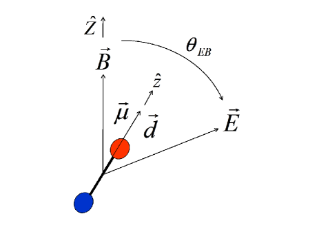
Figure 1: (Color online) Schematic electric and magnetic dipole moments for an OH molecule in a Hund’s case (a) scheme, in the presence of an arbitrary electric and magnetic field configuration $\vec{E},\vec{B},\theta_{EB}$.

When a magnetic field is applied, the interaction of the molecule with the field is given by the Zeeman Hamiltonian $H_{\rm{Z}}=-\vec{\mu}\cdot\vec{{B}}$. In the Hund’s case (a) basis set $|j,m_{j},\omega_{j}\rangle$ (we ignore the spectator ket $|\lambda,\sigma\rangle$ in the following unless stated otherwise and we take $\omega_{j}=\omega_{j}^{\prime}$), it takes the form

$$\langle j,m_{j},\omega_{j}|\,H_{\rm{Z}}\,|j^{\prime},m_{j}^{\prime},\omega_{j}\rangle=-\mu\,{B}\\ (-1)^{m_{j}-\omega_{j}}\,\sqrt{2j+1}\,\sqrt{2j^{\prime}+1}\\ \left(\begin{array}[]{ccc}j&1&j^{\prime}\\ -\omega_{j}&0&\omega_{j}\end{array}\right)\left(\begin{array}[]{ccc}j&1&j^{\prime}\\ -m_{j}&0&m_{j}^{\prime}\end{array}\right)$$ (1)

with $\mu=-\mu_{B}\,(g_{s}\sigma+g_{l}\lambda)$. Here we choose $\vec{{B}}$ to point along the space-fixed frame axis $\hat{Z}$ (as shown in Fig. 1). Based on the symmetry of the three-$j$ symbols, we must have $j^{\prime}-j=\Delta j=0,\pm 1$, $m_{j}^{\prime}=m_{j}$.

When an electric field is applied, the interaction of the molecule with the field is given by the Stark Hamiltonian $H_{\rm{S}}=-\vec{d}\cdot\vec{{E}}$ and in the Hund’s case (a) basis set, it takes the form

$$\langle j,m_{j},\omega_{j}|\,H_{\rm{S}}\,|j^{\prime},m_{j}^{\prime},\omega_{j}\rangle\\ =-d\,{E}\,\sqrt{\frac{4\pi}{3}}Y_{1,m_{j}^{\prime}-m_{j}}(\theta_{EB},\phi_{EB})\\ (-1)^{m_{j}-\omega_{j}}\,\sqrt{2j+1}\,\sqrt{2j^{\prime}+1}\\ \left(\begin{array}[]{ccc}j&1&j^{\prime}\\ -\omega_{j}&0&\omega_{j}\end{array}\right)\left(\begin{array}[]{ccc}j&1&j^{\prime}\\ -m_{j}&m_{j}-m_{j}^{\prime}&m_{j}^{\prime}\end{array}\right)$$ (2)

if we allow $\vec{{E}}$ to point in an arbitrary direction $(\theta_{EB},\phi_{EB})$ from the $\hat{Z}$ axis (as shown in Fig. 1). In the following we will set $\phi_{EB}=0$. From the three-$j$ symbols, we must have again $j^{\prime}-j=\Delta j=0,\pm 1$. But now, if there is a nonzero angle $\theta_{EB}$ between the $\vec{{E}}$ field and the $\vec{{B}}$ field, we have in general $m_{j}^{\prime}-m_{j}=0,\pm 1$. Thus the quantum numbers $m_{j}$ referred to a particular axis (the $\vec{{B}}$ or the $\vec{{E}}$ axis) are no longer good. Good quantum numbers can be found along two particular axes as shown in Ref. Bohn_MP_2013 , but we do not do so here. Note that if $\theta_{EB}=\pi/2$, $m_{j}^{\prime}=m_{j}\pm 1$ and if $\theta_{EB}=0$, we recover the case $m_{j}^{\prime}=m_{j}$.

In the absence of rotation, molecules with the quantum numbers $\lambda=\pm 1$ have the same energy causing a Lambda-doubling degeneracy for $\lambda\geq 1$. An additional term $H_{\lambda}$ stemming from the coupling of the rotation and the electronic angular momentum of the molecule splits this Lambda-doubling into two distinct states e and f of different parity Brown_Carrington_Book_2003 . A good basis set is then the parity basis set

$$|j,m_{j},|\omega_{j}|,\epsilon\rangle\,||\lambda|,|\sigma|\rangle=\dfrac{1}{\sqrt{2}}\,\bigg{\{}|j,m_{j},\omega_{j}\rangle\,|\lambda,\sigma\rangle\\ +\epsilon\,|j,m_{j},-\omega_{j}\rangle\,|-\lambda,-\sigma\rangle\bigg{\}}$$ (3)

with $\epsilon=\pm 1$ corresponding respectivelly to the e/f states parities Lara_PRA_78_033433_2008 . For OH, the f/e splitting is about $\Delta\approx 80$ mK and is diagonal in the parity basis,

$$\langle j,m_{j},|\omega_{j}|,\epsilon|\,H_{\Lambda}\,|j^{\prime},m_{j}^{\prime},|\omega_{j}|,\epsilon^{\prime}\rangle=\\ (-\epsilon)\,\Delta/2\ \delta_{j,j^{\prime}}\,\delta_{m_{j},m_{j}^{\prime}}\,\delta_{\epsilon,\epsilon^{\prime}}.$$ (4)

The Zeeman expression (1) in this new basis set is given by

$$\langle j,m_{j},|\omega_{j}|,\epsilon|\,H_{\rm{Z}}\,|j^{\prime},m_{j}^{\prime},|\omega_{j}|,\epsilon^{\prime}\rangle=-\mu\,{B}\ \delta_{\epsilon,\epsilon^{\prime}}\\ (-1)^{m_{j}-|\omega_{j}|}\,\sqrt{2j+1}\,\sqrt{2j^{\prime}+1}\\ \left(\begin{array}[]{ccc}j&1&j^{\prime}\\ -|\omega_{j}|&0&|\omega_{j}|\end{array}\right)\left(\begin{array}[]{ccc}j&1&j^{\prime}\\ -m_{j}&0&m_{j}^{\prime}\end{array}\right)$$ (5)

with $\mu=-\mu_{B}\,(g_{s}|\sigma|+g_{l}|\lambda|)\approx-2\,\mu_{B}$. The magnetic field mixes states of the same parity $\epsilon=\epsilon^{\prime}$ only. The Stark expression (2) is given by

$$\langle j,m_{j},|\omega_{j}|,\epsilon|\,H_{\rm{S}}\,|j^{\prime},m_{j}^{\prime},|\omega_{j}|,\epsilon^{\prime}\rangle=-d\,{E}\,\ (1-\delta_{\epsilon,\epsilon^{\prime}})\\ \sqrt{\frac{4\pi}{3}}Y_{1,m_{j}^{\prime}-m_{j}}(\theta_{EB},\phi_{EB})\\ (-1)^{m_{j}-\omega_{j}}\,\sqrt{2j+1}\,\sqrt{2j^{\prime}+1}\\ \left(\begin{array}[]{ccc}j&1&j^{\prime}\\ -|\omega_{j}|&0&|\omega_{j}|\end{array}\right)\left(\begin{array}[]{ccc}j&1&j^{\prime}\\ -m_{j}&m_{j}-m_{j}^{\prime}&m_{j}^{\prime}\end{array}\right)$$ (6)

The electric field mixes states of the different parity $\epsilon\neq\epsilon^{\prime}$ only. The selection rules $\Delta j=0,\pm 1$ and $\Delta m_{j}=0,\pm 1$ still hold. In the following, we take $j=j^{\prime}=3/2$.

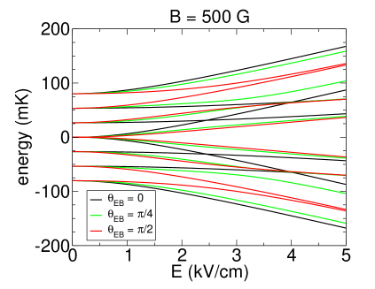
Figure 2: (Color online) Eigenenergies of the ground state OH molecule in combined electric and magnetic fields as a function of the electric field for $\theta_{EB}=0$ (black curve), $\theta_{EB}=\pi/4$ (green curve), $\theta_{EB}=\pi/2$ (red curve). The magnetic field is $B=500$ G.

The diagonalization of the molecular Hamiltonian $H_{\lambda}+H_{\rm{Z}}+H_{\rm{S}}$ in the parity basis set given by the expressions (4), (5), and (6) leads to the eight eigenenergies denoted $\varepsilon_{i}$ with $i=1,...,8$ from lowest to highest energy; and eigenfunctions denoted $|i\rangle$ of the OH molecule in a combined electric and magnetic field with a relative orientation $\theta_{EB}$. These energies are shown in Fig. 2 for a fixed magnetic field of $B=500$ G as a function of the electric field $E$ for the three angles $\theta_{EB}=0$ (black curves, parallel fields), $\theta_{EB}=\pi/4$ (green curves, neither parallel, nor perpendicular), and $\theta_{EB}=\pi/2$ (red curves, perpendicular fields).

For the highest excited adiabatic state $|8\rangle$ represented by the highest energy curve, it is easier to induce an electric dipole moment when the electric field is more parallel to the magnetic field axis while it is harder when the fields are more perpendicular. This can be seen from the derivative of the energy curves with respect to the electric field which is proportional to the induced electric dipole moment. The derivative for the $\theta_{EB}=\pi/2$ red curve is smaller than that for the $\theta_{EB}=0$ black curve, the one for the $\theta_{EB}=\pi/4$ green curve sitting in between. In terms of the results of Ref. Bohn_MP_2013 , the induced electric dipole moment $\tilde{d}$ for the upper adiabatic state $|8\rangle$ can be approximated by

$$\tilde{d}\approx\frac{|\omega_{j}m_{j}|}{j(j+1)}\left(1+\frac{\mu B}{dE}\cos(\theta_{EB})\right)\,d.$$ (7)

Then, if $\theta_{EB}$ goes from 0 to $\pi/2$, $\tilde{d}$ decreases in magnitude for fixed $B$ and $E$ fields as seen on Fig. 2.

II.2 Molecular scattering

In what follows we will be concerned with molecules colliding in their stretched states $|8\rangle$, which are magnetically trapped. In collisions, these molecules will exert torques on one another that can disturb their orientation, producing molecules in states $|i<8\rangle$ and in general leading to trap loss and heating. As these appear to be the dominant loss collisions Stuhl_N_492_396_2012 , we focus on them and ignore the possibility of chemical reactions. Our scattering theory is therefore similar to the long-range-dominated theories in Refs. Avdeenkov_PRA_64_052703_2001 ; Tscherbul_NJP_11_055021_2009 .

We consider two OH molecules of mass $m_{1},m_{2}$ and position $\vec{r}_{1},\vec{r}_{2}$ respectively. We decouple the motion of the two-body system into a motion of a center of mass, of total mass $m_{\text{tot}}=m_{1}+m_{2}$ and position $\vec{R}=(m_{1}\vec{r}_{1}+m_{2}\vec{r}_{2})/(m_{1}+m_{2})$, and a motion of a relative particle, of reduced mass $m_{\text{red}}=(m_{1}m_{2})/(m_{1}+m_{2})$ and position $\vec{r}=\vec{r}_{2}-\vec{r}_{1}$. The total Hamiltonian of the relative motion is $H=T+V$ with $T$ being the relative kinetic energy operator of the relative motion and $V$ the potential energy. The long-range electric dipole-dipole interaction is given by

$$V=\frac{{\vec{d}_{1}}\cdot{\vec{d}_{2}}-3({\vec{d}_{1}}\cdot\hat{r})({\vec{d}_{2}}\cdot\hat{r})}{4\pi\varepsilon_{0}r^{3}}.$$ (8)

We do not consider the magnetic dipole-dipole interaction since it is of the order of $\alpha^{2}\approx 10^{-4}$ smaller than the electric dipole-dipole interaction. Because the molecules are identical (same isotope, same mass), we construct an overall wavefunction $\Psi$ of the system for which the molecular permutation operator $P$ gives $P\,\Psi=\epsilon_{P}\,\Psi$ with $\epsilon_{P}=+1$ for bosonic molecules and $\epsilon_{P}=-1$ for fermionic molecules. In this study, we consider ¹⁶OH bosonic molecules so that $\epsilon_{P}=+1$. This is due to a total spin $\vec{f}=\vec{j}+\vec{i}$ with integer quantum numbers $f=1,2$, where $\vec{i}$ is the nuclear spin of the molecule ($i=1/2$) and $\vec{j}$ the total angular momentum ($j=3/2$) of the molecule considered. We assume that the nuclear spin $i$ and the angular momentum $j$ are decoupled. This is a good approximation for strong magnetic fields ($\mu B\gg\Delta_{\text{hf}}$) or high collision energies ($E_{c}\gg\Delta_{\text{hf}}$) where $\Delta_{\text{hf}}\approx 4$ mK is the hyperfine energy splitting between the $f=1$ and $f=2$ manifolds. For the state we consider, this assumption is valid for most of the results presented here especially when $B\gg 100$ G. Note that the hyperfine structure was previously considered in OH cold collisions that focused on smaller collision energies and smaller magnetic fields Avdeenkov_PRA_66_052718_2002 ; Ticknor_PRA_71_022709_2005 .

Figure 3: (Color online) Adiabatic energies correlating to the $|8\rangle+|8\rangle$ combined molecular state as a function of the intermolecular separation $r$, for $\theta_{EB}=0$ (black curve), $\theta_{EB}=\pi/4$ (green curve), $\theta_{EB}=\pi/2$ (red curve) and for different electric fields (thin solid: $E=0$ kV/cm, dashed: $E=2$kV/cm, thick solid: $E=3$ kV/cm). The magnetic field is $B=500$ G.

We construct symmetrized states of the internal wavefunction of the combined molecular states $|i_{1}\rangle\,|i_{2}\rangle$ of two OH molecules with energies $\varepsilon_{i_{1}}+\varepsilon_{i_{2}}$ ($i_{1},i_{2}=1,...,8$)

$$|i_{1},i_{2},\eta\rangle=\frac{1}{\sqrt{2(1+\delta_{i_{1},i_{2}})}}\bigg{[}|i_{1},i_{2}\rangle+\eta|i_{2}\,i_{1}\rangle\bigg{]}$$ (9)

for which $P\,|i_{1},i_{2},\eta\rangle=\eta\,|i_{1},i_{2},\eta\rangle$. $\eta$ is a good quantum number and is conserved during the collision. If the molecules are in the same molecular internal state, only the symmetry $\eta=+1$ has to be considered. If they are in different internal state, both symmetries $\eta=\pm 1$ have to be considered. As we consider both initial OH molecules in their highest eigenstate $|8\rangle$ in the combined electric and magnetic field, the molecules are indistinguishable and $\eta=+1$. The total wavefunction $\Psi(\vec{r})$ with $\vec{r}=\{r,\theta,\varphi\}$ is expanded onto a basis set of spherical harmonics $Y_{l,m_{l}}(\theta,\varphi)$ corresponding to the orbital angular momentum of the colliding particles

$$\Psi_{k}(r,\theta,\varphi) = \sum_{k^{\prime\prime}=1}^{N_{\text{tot}}}\frac{1}{r}\,F_{k^{\prime\prime}k}(r)\,Y_{l^{\prime\prime},m_{l}^{\prime\prime}}(\theta,\varphi)\,|i_{1}^{\prime\prime}\,i_{2}^{\prime\prime},\eta^{\prime\prime}\rangle$$ (10)

$$= \sum_{k^{\prime\prime}=1}^{N_{\text{tot}}}\frac{1}{r}\,F_{k^{\prime\prime}k}(r)\,|i_{1}^{\prime\prime}\,i_{2}^{\prime\prime},l^{\prime\prime},m_{l}^{\prime\prime},\eta^{\prime\prime}\rangle.$$

where $k=i_{1},i_{2},l,m_{l},\eta$ and $N_{\text{tot}}$ is the total number of diabatic channels we use in our calculation.

Symmetry consideration can restrict the number of channels required. Because $\eta=+1$, and to satisfy $P\,\Psi=\epsilon_{P}\,\Psi$ with $\epsilon_{P}=+1$, $l$ must take even values. In this study we consider only the partial waves $l=0,2,4,6,8$, finding these sufficient to converge the results at the collision energies investigated here. The total number of channels is typically $N_{\text{tot}}=1620$. Moreover, when the fields are parallel, the total quantum number $M=m_{j_{1}}+m_{j_{2}}+m_{l}$ is conserved, and $N_{\text{tot}}=118$ for the $M=+3$ components for the initial states $m_{j_{1}}=3/2$, $m_{j_{2}}=3/2$, $m_{l}=0$ for example. The total energy $E$ is equal to the sum $\varepsilon_{i_{1}}+\varepsilon_{i_{2}}+E_{c}$, where $E_{c}$ is the initial collision energy. The total energy $E$ is conserved during the collision. We choose the zero of energy to be equal to $\varepsilon_{8}+\varepsilon_{8}$, the energy of our initial molecular states. The time-independent Schrödinger equation $H\Psi=E\Psi$ provides a diabatic set of close-coupling differential equations for the radial functions $F_{k^{\prime}k}(r)$ from a state $k$ to a state $k^{\prime}$

$$\left\{-\frac{\hbar^{2}}{2m_{\text{red}}}\frac{d^{2}}{dr^{2}}+\frac{\hbar^{2}\,l(l+1)}{2m_{\text{red}}r^{2}}-E\right\}\,F_{k^{\prime}k}(r)\\ +\sum_{k^{\prime\prime}=1}^{N_{\text{tot}}}{\cal U}_{k^{\prime}k^{\prime\prime}}(r)\ F_{k^{\prime\prime}k}(r)=0$$ (11)

where

$${\cal U}_{k^{\prime}k^{\prime\prime}}(r)=\langle i_{1}^{\prime},i_{2}^{\prime},l^{\prime},m_{l}^{\prime},\eta^{\prime}|\,V_{\text{dd}}\,|i_{1}^{\prime\prime},i_{2}^{\prime\prime},l^{\prime\prime},m_{l}^{\prime\prime},\eta^{\prime\prime}\rangle.$$ (12)

Using Eq. (9) and the fact that the individual molecular eigenstates $|i_{1}\rangle$ and $|i_{2}\rangle$ in Eq.(3) are linear combinations of the basis set $|j_{1},m_{j_{1}},|\omega_{j_{1}}|,\epsilon\rangle$ and $|j_{2},m_{j_{2}},|\omega_{j_{2}}|,\epsilon\rangle$ after diagonalisation, we can obtain the coupling matrix elements ${\cal U}_{k^{\prime}k^{\prime\prime}}(r)$ knowing that the dipole-dipole interaction in the Hund’s case (a) molecule-molecule basis set $|j_{1},m_{j_{1}},\omega_{j_{1}},j_{2},m_{j_{2}},\omega_{j_{2}},l,m_{l}\rangle$ is expressed by

$$\langle j_{1},m_{j_{1}},\omega_{j_{1}},j_{2},m_{j_{2}},\omega_{j_{2}},l,m_{l}|\\ \,V_{\text{dd}}\,|j_{1}^{\prime},m_{j_{1}}^{\prime},\omega_{j_{1}},j_{2}^{\prime},m_{j_{2}}^{\prime},\omega_{j_{2}},l^{\prime},m_{l}^{\prime}\rangle\\ =-\frac{\sqrt{30}\,d_{1}d_{2}}{4\pi\varepsilon_{0}r^{3}}\,(-1)^{m_{j_{1}}-\omega_{j_{1}}}\,(-1)^{m_{j_{2}}-\omega_{j_{2}}}\,(-1)^{m_{l}}\\ \sqrt{2j_{1}+1}\,\sqrt{2j_{2}+1}\,\sqrt{2l+1}\\ \sqrt{2j_{1}^{\prime}+1}\,\sqrt{2j_{2}^{\prime}+1}\,\sqrt{2l^{\prime}+1}\\ \sum_{p=-2}^{2}\,\sum_{p_{1}=-1}^{1}\,\sum_{p_{2}=-1}^{1}\,\left(\begin{array}[]{ccc}1&1&2\\ p_{1}&p_{2}&-p\end{array}\right)\\ \,\left(\begin{array}[]{ccc}j_{1}&1&j_{1}^{\prime}\\ -\omega_{j_{1}}&0&\omega_{j_{1}}\end{array}\right)\,\left(\begin{array}[]{ccc}j_{1}&1&j_{1}^{\prime}\\ -m_{j_{1}}&m_{j_{1}}-m_{j_{1}}^{\prime}&m_{j_{1}}^{\prime}\end{array}\right)\\ \,\left(\begin{array}[]{ccc}j_{2}&1&j_{2}^{\prime}\\ -\omega_{j_{2}}&0&\omega_{j_{2}}\end{array}\right)\,\left(\begin{array}[]{ccc}j_{2}&1&j_{2}^{\prime}\\ -m_{j_{2}}&m_{j_{2}}-m_{j_{2}}^{\prime}&m_{j_{2}}^{\prime}\end{array}\right)\\ \,\left(\begin{array}[]{ccc}l&2&l^{\prime}\\ 0&0&0\end{array}\right)\,\left(\begin{array}[]{ccc}l&2&l^{\prime}\\ -m_{l}&m_{l}-m_{l}^{\prime}&m_{l}^{\prime}\end{array}\right).$$ (13)

The multichannel interaction is illustrated in Fig. 3 by showing the lowest adiabatic energies of the symmetrized combined molecular state $|8,8,\eta=+1\rangle$ as a function of $r$ at a magnetic field of $B=500$ G, for the electric fields $E=0,2,3$ kV/cm and different orientations $\theta_{EB}=0,\pi/4,\pi/2$. These curves are obtained by diagonalizing the matrix ${\cal U}(r)$ for each $r$. The thin solid black line shows the result for zero electric field $E=0$ kV/cm illustrating its repulsive $C_{6}/r^{6}$ behavior Stuhl_N_492_396_2012 . When the electric field is turned on, second-order perturbations induce an attractive $C_{4}/r^{4}$ Avdeenkov_PRA_66_052718_2002 ; Quemener_PRA_84_062703_2011 coming from a mixing of the $l=0$ and $l=2$ partial waves of the dipole-dipole interaction. This interaction becomes increasingly attractive as the electric field grows, and also when the magnetic field is more parallel to the electric field. This fact follows qualitatively from the induced electric dipoles of these state, as discussed for Fig. 2: for perpendicular fields, the electric dipole moment is harder to induce hence a weaker attractive $C_{4}/r^{4}$ interaction, while for parallel fields the reverse is true.

The set of coupled equations Eq. (11) is solved for each $r$ using a diabatic method, using the standard method of the propagation of the log-derivative matrix Johnson_JCP_13_445_1973 . Matching the log-derivative matrix with asymptotic solutions at large $r$ yields finally the scattering matrix $S$ and the elastic and total inelastic cross sections and rate coefficients, which are shown in the next section. Note that ab initio calculations are not precise enough at such cold temperatures ($T\leq 1$ K) to rule out the presence of a potential energy barrier in the entrance channel that could prevent the chemical reaction OH +OH $\to$ O + H₂O to occur Ge_ACP_855_253_2006 . As a consequence, we do not consider the possibility of chemical reactions in the present study but could be considered in future works by using an absorbing condition at short range for example Quemener_PRA_84_062703_2011 .

III Application to cold and ultracold OH + OH molecular scattering

To better orient the discussion of scattering, consider the scales of electric and magnetic fields as seen by the OH molecule. For a prototypical cold collision energy $E=1$mK, this energy is the same as the Stark energy $|\vec{d}\cdot\vec{E}|$ for a dipole moment $|\vec{d}|=1.67$ D and an electric field $E=0.0247$ kV/cm, and it is the same as the Zeeman energy $|\vec{\mu}\cdot\vec{B}|$ for a dipole moment $|\vec{\mu}|=2\,\mu_{B}$ in a magnetic field $B=7.4$ G. As a rule of thumb, one might therefore expect the magnetic field to have a dominant effect when $B/E\gg 300$ G/(kV/cm), and the electric field to have a dominant effect when the reverse is true.

The prospect of manipulating collisions via both electric and magnetic fields, possibly pointing in different directions, to say nothing of different collision energies, opens a large parameter space to consider. In this section we will explore different slices through this parameter space, by varying separately the electric field magnitude, the magnetic field magnitude, and the relative orientation of the fields.

III.1 Scattering versus electric field

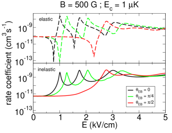
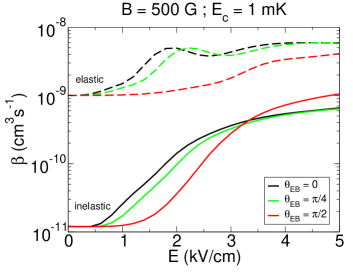
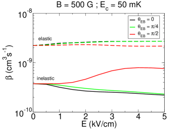
Figure 4: (Color online) Rate coefficients as a function of electric field for $\theta_{EB}=0$ (black curve), $\theta_{EB}=\pi/4$ (green curve), $\theta_{EB}=\pi/2$ (red curve). The collision energy is $E_{c}=1\mu$ K (top pannel), $E_{c}=1$ mK (middle pannel), $E_{c}=50$ mK (bottom pannel). The magnetic field is fixed to $B=500$ G. Elastic process are plotted in dashed lines, inelastic processes are plotted in solid lines.

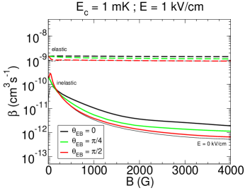
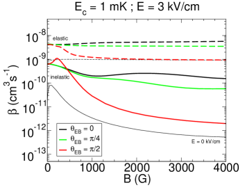
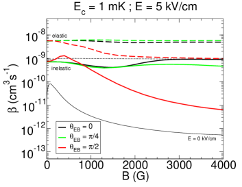
Figure 5: (Color online) Rate coefficients as a function of magnetic field for $\theta_{EB}=0$ (black curve), $\theta_{EB}=\pi/4$ (green curve), $\theta_{EB}=\pi/2$ (red curve). The electric field is $E=1$ kV/cm (top panel), $E=3$ kV/cm (middle panel), $E=5$ kV/cm (bottom panel). The collision energy is fixed to $E_{c}=1$ mK. The thin solid line black line corresponds to $E=0$ kV/cm. Elastic process are plotted in dashed lines, inelastic processes are plotted in solid lines.

The general effect of increasing the electric field on scattering of OH is to increase the inelastic scattering rate. This effect arises because electric dipoles are induced, which exert the long-range torques on one another that drive state-changing collisions Avdeenkov_PRA_66_052718_2002 . This effect is seen in Fig. 4 , which shows the electric field dependence of the elastic and inelastic rate coefficients for $\theta_{EB}=0$ (black curves), $\theta_{EB}=\pi/4$ (green curves), and $\theta_{EB}=\pi/2$ (red curves) at different magnitude of collision energy, for a fixed magnetic field $B=500$ G. The three panels denote three different collision energies. At an ultra-low collision energy of $E_{c}=1\,\mu$ K, the rate coefficients show the presence of resonances, signaling the occurrence of long-range, “field-linked” resonance states predicted in Ref. Avdeenkov_PRA_66_052718_2002 . They correspond to the coincidence of virtual states with the collision energy as the electric field is turned on and as the adiabatic energy curves become more attractive (seen on Fig. 3).

The electric field values at which these resonances appear clearly depends on the angle $\theta_{EB}$ between the fields. As noted above, for more parallel fields it is easier to induce the electric dipole moments of the molecules and to obtain strong attractive interaction curves, hence resonances appear at lower electric fields. Vice versa, for more perpendicular fields the same resonances appear at higher electric fields since it is harder to induce the electric dipole moments and to obtain attractive interaction curves. Because of these resonances, the inelastic processes can be decreased by three orders of magnitude (see for instance at $E=1$ kV/cm) between the parallel and perpendicular cases. The overall trend is a rise of the rates with the electric fields due to the increased dipolar coupling with other inelastic states as the electric field is turned on.

At a somewhat higher collision energy of $E_{c}=1$ mK, the resonances are smoothed out since the width of scattering resonances usually increases as the collision energy increases Mayle_PRA_87_012709_2013 . The rise of the rates with the electric field is still visible. According to our rule of thumb, the electric field should exceed $\sim 1.7$ kV/cm to exert a stronger influence on the molecules than a 500 G magnetic field. And indeed, the second and third panels of Figure. 4 show suppressed inelastic rates blow about this field, and enhanced rates above it. Details of the fields still matter, however. At still larger collisions energy, 50 mK, inelastic rates continue to be suppressed at high electric field, when the fields are not perpendicular.

III.2 Scattering versus magnetic field

As opposed to electric fields, magnetic fields tend to decrease the rate of inelastic scattering. This decrease is tied to the general separation of molecular states in a field, which reduces the Franck-Condon factors between initial and final states Ticknor_PRA_71_022709_2005 . This effect, including its modifications due to the electric field, are shown in Fig. 5. This figure presents the magnetic field dependence of the elastic and inelastic rate coefficients for $\theta_{EB}=0$ (black curves), $\theta_{EB}=\pi/4$ (green curves), and $\theta_{EB}=\pi/2$ (red curves) for a fixed collision energy of $E_{c}=1$ mK. In this figure each panel shows the result at a different electric field. The $E=0$ kV/cm case is represented in thin black line and of course does not depend on $\theta_{EB}$.

The elastic rates are independent of the magnetic field while the inelastic rates decrease with the magnetic field, in agreement with previous results of Ref. Ticknor_PRA_71_022709_2005 . Considering the overall trends, our rule of thumb would suggest that the magnetic-field suppression would become important at magnetic fields of 300 G, 900 G, and 1500 G, for the three panels, respectively, and this is approximately what is seen. For $E=1$ kV/cm, the trends of the rates are comparable and do not differ so much from the zero field case. The electric field generates the largest deviation from the field-free case when the fields are parallel.

Once the electric field is larger, the angle between fields plays a more significant role. For $E=3$ kV/cm, the rates of the $\theta_{EB}=0$ and $\theta_{EB}=\pi/4$ case have globally increased with the electric field and show a moderate magnetic field dependence while the rates of the $\theta_{EB}=\pi/2$ have increased but still show a magnetic field dependence similar to lower electric fields. This is because the electric field is not strong enough for the perpendicular case to polarize the electric dipole moment and inelastic rates are still suppressed. Finally for $E=5$ kV/cm, the $\theta_{EB}=0$ and $\theta_{EB}=\pi/4$ cases show a weak magnetic dependence while $\theta_{EB}=\pi/2$ still shows a certain dependence. For this case, one can see here that for strong magnetic fields, one needs strong electric fields to get a strong electric dipole-dipole interaction to increases the inelastic rates.

III.3 Scattering versus the relative field orientations

Fig. 6 presents the rate coefficient for different electric fields at a fixed magnetic field $B=1500$ G and collision energy $E_{c}=1$ mK, as a function of the fields angle $\theta_{EB}$. For an electric field of $E=1$ kV/cm, elastic and inelastic collisions depend weakly on the angle the electric field makes with respect to the magnetic field. The electric field is not strong enough to play a significant role since $B/E\gg 300$ G/(kV/cm). Even though, we see that the fields angle can have some effect on the inelastic rates, within a factor of 2 to 3. For an increased electric field of $E=3$ kV/cm, the overall rates have increased from the low electric field case but they decrease from $\theta_{EB}=0$ to $\theta_{EB}=\pi/2$ showing a strong anisotropy. Recall that in parallel fields, the magnetic field helps to polarize the molecules, increasing the inelastic rates. Molecular collisions highly depend on the relative angle of the fields. For the same magnetic field, they can differ by one order of magnitude for the inelastic processes for example. Finally at $E=5$ kV/cm, where electric fields have an effect comparable to magnetic fields ($B/E=300$ G/(kV/cm)), the inelastic rates are large and the angle dependence starts to weaken compared to the previous case of $E=3$ kV/cm. In this case the electric field is strong enough to polarize the molecules along itself, so the strength and direction of the magnetic field starts to become irrelevant.

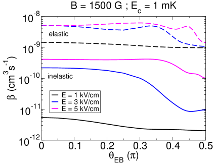
Figure 6: (Color online) Rate coefficients as a function of the fields orientation for $E=1$ kV/cm (black curve), $E=3$ kV/cm (blue curve), $E=5$ kV/cm (pink curve). The magnetic field is $B=1500$ G and the collision energy is $E_{c}=1$ mK. Elastic process are plotted in dashed lines, inelastic processes are plotted in solid lines.

III.4 Links with experiments

In experiments, polar molecules of OH are trapped in a magnetic quadrupole trap with spatially varying magnetic fields Stuhl_N_492_396_2012 , and can be simultaneously subject to a uniform electric field Stuhl_MP_2013 . At each location of the molecules in the trap, therefore, the molecules experience crossed fields of arbitrary magnitude and relative orientation, hence different outcomes of two-body collisions as previously seen in this study. The fact that collision processes highly depend on the position in the trap can be used to create non-uniform configurations of electric fields in magnetic traps so that high value of $\theta_{\text{EB}}$ regions will favor elastic collisions while low value regions will favor inelastic ones. With proper field configurations, this could be used as a knife for evaporative cooling in such traps in order to remove the particles with the higher energy and keep the particles with the lower energy.

In such traps, it is somewhat more complicated to give an overall rate coefficient for a given temperature and for a given electric field since the molecular rate coefficients depend on the position of the trap as well as the collision energy. Experimental data of inelastic loss are now available for collision of OH molecules in a quadrupole trap and uniform electric fields Stuhl_MP_2013 . To confront these data with theoretical predictions, one needs to consider the position and velocity dependent rate coefficients along with the proper phase space distributions of molecular positions and velocities to describe molecular losses as a function of time. The option to consider or not the possibility of chemical reactions for OH + OH collisions will also play a role on the overall magnitude of the loss rates (inelastic + reactive processes). This has to be kept in mind when comparing with experimental results.

In addition, one also needs to consider the time dynamics of the molecules inside the trap between collisions, since elastic rates are higher than the inelastic ones so that rethermalization plays an important role and since elastic scattering re-distributes the velocities directions and magnitudes of the molecules according to the differential cross sections after a collision. Such calculations are more complex and usually require Monte-Carlo simulations using classical trajectories Barletta_NJP_12_113002_2010 ; Wu_PRA_56_560_1997 . This is beyond the scope of this paper and will be investigated in future work.

IV Conclusion

We have studied the collisions of electric and magnetic polar molecules in arbitrary configurations of electric and magnetic fields, taking the OH molecules as an example. The electric dipolar interaction depends on the way the electric dipole moments are induced. For the state considered in this study, it is easier to induce the electric dipoles when the electric and magnetic fields are parallel and this increases the strength of the molecule-molecule electric dipolar interaction. When the fields become perpendicular, it is harder to induce the electric dipoles along the electric field axis since the magnetic field tends also to align the molecular axis with it. This moderates the strength of the electric dipolar interaction. This is seen in the dynamics of OH + OH collisions where we found a strong dependence of the rate coefficients of elastic and inelastic processes on the electric and magnetic field configurations. For example, more parallel fields increase the inelastic processes while more perpendicular fields moderate them. If the polar molecules are confined in a magnetic quadrupole trap in the presence of an electric field, the molecular collisions will be space and velocity dependent. Therefore the molecular dynamics in such traps is complex. Elastic and inelastic collisions have to be taken into account as well as the motion of the particles between collisions in order to describe molecular loss and thermalization. This will be left for future investigations.

References

- (1) G. Quéméner and P. S. Julienne, Chem. Rev. 112, 4949 (2012)
- (2) K.-K. Ni, S. Ospelkaus, M. H. G. de Miranda, A. Pe’er, B. Neyenhuis, J. J. Zirbel, S. Kotochigova, P. S. Julienne, D. S. Jin, and J. Ye, Science 322, 231 (2008)
- (3) S. Ospelkaus, K.-K. Ni, D. Wang, M. H. G. de Miranda, B. Neyenhuis, G. Quéméner, P. S. Julienne, J. L.Bohn, D. S. Jin, and J. Ye, Science 327, 853 (2010)
- (4) K.-K. Ni, S. Ospelkaus, D. Wang, G. Quéméner, B. Neyenhuis, M. H. G. de Miranda, J. L. Bohn, D. S. Jin, and J. Ye, Nature 464, 1324 (2010)
- (5) M. H. G. de Miranda, A. Chotia, B. Neyenhuis, D. Wang, G. Quéméner, S. Ospelkaus, J. Bohn, J. L. Ye, and D. S. Jin, Nature Physics 7, 502 (2011)
- (6) A. Chotia, B. Neyenhuis, S. A. Moses, B. Yan, J. P. Covey, M. Foss-Feig, A. M. Rey, D. S. Jin, and J. Ye, Phys. Rev. Lett. 108, 080405 (2012)
- (7) E. S. Shuman, J. F. Barry, and D. DeMille, Nature 467, 820 (2010)
- (8) B. K. Stuhl, M. T. Hummon, M. Yeo, G. Quéméner, J. L. Bohn, and J. Ye, Nature 492, 396 (2012)
- (9) T. V. Tscherbul and R. V. Krems, J. Chem. Phys. 125, 194311 (2006)
- (10) E. Abrahamsson, T. V. Tscherbul, and R. V. Krems, J. Chem. Phys. 127, 044302 (2007)
- (11) T. V. Tscherbul, J. Chem. Phys. 128, 244305 (2008)
- (12) T. V. Tscherbul, J. Klos, L. Rajchel, and R. V. Krems, Phys. Rev. A 75, 033416 (2007)
- (13) A. V. Avdeenkov and J. L. Bohn, Phys. Rev. A 66, 052718 (2002)
- (14) C. Ticknor and J. L. Bohn, Phys. Rev. A 71,022709 (2005)
- (15) T. V. Tscherbul, Y. V. Suleimanov, V. Aquilanti, and R. V. Krems, New J. Phys. 11, 055021 (2009)
- (16) J. Perez-Rios, J. Campos-Martinez, and M. I. Hernandez, J. Chem. Phys. 134, 124310 (2011)
- (17) L. M. C. Janssen, P. S. Zuchowski, A. van der Avoird, G. C. Groenenboom, and J. M. Hutson, Phys. Rev. A 83, 022713 (2011)
- (18) Y. V. Suleimanov, T. V. Tscherbul, and R. V. Krems, J.Chem. Phys. 137, 024103 (2012)
- (19) L. M. C. Janssen, A. van der Avoird, and G. C. Groenenboom, Phys. Rev. Lett. 110, 063201 (2013)
- (20) B. K. Stuhl, M. Yeo, M. T. Hummon, and J. Ye, Mol. Phys. (2013) ; published online at http://dx.doi.org/10.1080/00268976.2013.793838
- (21) A. V. Gorshkov, S. R. Manmana, G. Chen, J. Ye, E. Demler, M. D. Lukin, and A. M. Rey, Phys. Rev. Lett. 107, 115301 (2011)
- (22) M. A. Baranov, M. Dalmonte, G. Pupillo, and P. Zoller, Chem. Rev. 112, 5012 (2012)
- (23) M. L. Wall, E. Bekaroglu, and L. D. Carr, arXiv e-print 1212.3042 (2012)
- (24) J. M. Brown and A. Carrington, Rotational spectroscopy of diatomic molecules (Cambridge University Press, 2003)
- (25) J. L. Bohn and G. Quéméner, Mol. Phys. (2013) ; published online at http://dx.doi.org/10.1080/00268976.2013.783721
- (26) M. Lara, B. L. Lev, and J. L. Bohn, Phys. Rev. A 78, 033433 (2008)
- (27) A. V. Avdeenkov and J. L. Bohn, Phys. Rev. A 64, 052703 (2001)
- (28) G. Quéméner, J. L. Bohn, A. Petrov, and S. Kotochigova, Phys. Rev. A 84, 062703 (2011)
- (29) B. R. Johnson, J. Comp. Phys. 13, 445 (1973)
- (30) Y. Ge, K. Olsen, R. I. Kaiser, and J. D. Head, AIP Conf. Proc. 855, 253 (2006)
- (31) M. Mayle, G. Quéméner, B. P. Ruzic, and J. L. Bohn, Phys. Rev. A 87, 012709 (2013)
- (32) P. Barletta, J. Tennyson, and P. F. Barker, New J. Phys. 12, 113002 (2010)
- (33) H. Wu, E. Arimondo, and C. J. Foot, Phys. Rev. A 56, 560 (1997)