Controlling adsorption of semiflexible polymers on planar and curved substrates

Abstract

We study the adsorption of semiflexible polymers such as polyelectrolytes or DNA on planar and curved substrates, e.g., spheres or washboard substrates via short-range potentials using extensive Monte-Carlo simulations, scaling arguments, and analytical transfer matrix techniques. We show that the adsorption threshold of stiff or semiflexible polymers on a planar substrate can be controlled by polymer stiffness: adsorption requires the highest potential strength if the persistence length of the polymer matches the range of the adsorption potential. On curved substrates, i.e., an adsorbing sphere or an adsorbing washboard surface, the adsorption can be additionally controlled by the curvature of the surface structure. The additional bending energy in the adsorbed state leads to an increase of the critical adsorption strength, which depends on the curvature radii of the substrate structure. For an adsorbing sphere, this gives rise to an optimal polymer stiffness for adsorption, i.e., a local minimum in the critical potential strength for adsorption, which can be controlled by curvature. For two- and three-dimensional washboard substrates, we identify the range of persistence lengths and the mechanisms for an effective control of the adsorption threshold by the substrate curvature.

I Introduction

Typical synthetic polymers are flexible and effects from their bending rigidity can be neglected on length scales comparable to their contour length. For semiflexible polymers, on the other hand, the bending rigidity is relevant for large scale fluctuations. Many biopolymers such as DNA, filamentous (F-) actin, or microtubules belong to the class of semiflexible polymers. The biological function of these polymers requires considerable mechanical rigidity; for example, actin filaments are the main structural elements of the cytoskeleton, in which they form a network rigid enough to maintain the shape of the cell and to transmit forces. Prominent examples for synthetic semiflexible polymers are polyelectrolytes at sufficiently low salt concentration Skolnick and Fixman (1977) or dendronized polymers Förster et al. (1999), where the electrostatic repulsion of charges along the backbone or the steric interaction of side groups give rise to considerable bending rigidity.

The bending rigidity of semiflexible polymers is characterized by their bending rigidity $\kappa$. The ratio of bending rigidity and thermal energy determines the persistence length $L_{p}\sim\kappa/k_{B}T$, which is the characteristic length scale for the decay of tangent correlations Gutjahr, Lipowsky, and Kierfeld (2006). The physics of semiflexible polymers becomes qualitatively different from the physics of flexible synthetic polymers on length scales smaller than the persistence length where bending energy dominates over conformational entropy. Typical biopolymer persistence lengths range from $50\,{\rm nm}$ for DNA Bednar et al. (1995) (at high salt concentrations) to the $10\,{\rm\mu m}$-range for F-actin Ott et al. (1993) or even up to the mm-range for microtubules Venier et al. (1994) and are, thus, comparable to typical contour lengths.

Polymer adsorption is the most important phase transition for single polymer chains with numerous applications de Gennes (1979); Eisenriegler (1993); Netz and Andelman (2003). Here, we consider the adsorption of a single semiflexible polymer to a planar surface and investigate, in particular, how the bending rigidity allows to control the adsorption transition, i.e., to control the critical potential strength necessary for adsorption. Relevant adsorption interactions are van der Waals interactions or depletion interactions for uncharged semiflexible polymers and screened electrostatic interactions or counterion-induced interactions for charged polymers such as DNA or F-actin Angelini et al. (2003). F-actin can also be bound via crosslinking molecules. Dos Remedios et al. (2003); Winder and Ayscough (2005); Fletcher and Mullins (2010)

From a theoretical point of view, the adsorption of semiflexible polymers exhibits a rich behavior because several relevant length scales compete. For a free semiflexible polymer the persistence length $L_{p}$ and its contour length $L$ are the relevant length scales, and for $L<L_{p}$ the behavior is dominated by bending energy. In the adsorption problem, both length scales compete with the correlation length $\xi$ of the adsorption transition and the range $\ell$ of the adsorption potential. The correlation length $\xi$ is given by the characteristic length of desorbed segments (loops) and diverges at the adsorption transition. If the contour length is small compared to the correlation length, $L<\xi$, finite size effects are relevant and affect the critical behavior close to the adsorption transition. If the persistence length is small compared to the correlation length, $L_{p}<\xi$, there is a crossover in the critical properties of the adsorption transition to those of a flexible polymer Maggs, Huse, and Leibler (1989); Kierfeld (2006), which can only be observed close to the adsorption transition, and corrections to the critical potential strength are small. If the persistence length becomes even smaller than the potential range, $L_{p}\lesssim\ell$, we expect that the critical potential strength for adsorption itself will cross over to the flexible polymer result. This crossover is the central subject of this paper.

Various aspects of the adsorption transition of semiflexible polymers to planar substrates by short-range potentials have been studied theoretically. An early study of semiflexible polymer adsorption by Birshtein Birshtein, Zhulina, and Skvortsov (1979) was based on an analytical transfer matrix calculation for lattice polymers. The main finding was that the critical potential strength for adsorption decreases with stiffness, i.e., stiff polymers adsorb more easily, and that the transition sharpens with increasing stiffness but remains continuous. These findings were confirmed by numerical calculations van der Linden, Leermakers, and Fleer (1996). A decreasing critical potential strength for adsorption has also been found in off-lattice molecular dynamics simulations Kramarenko et al. (1996) and Monte-Carlo simulations Sintes, Sumithra, and Straube (2001). Scaling arguments for the critical potential strength for the adsorption of semiflexible polyelectrolytes Netz and Joanny (1999a) indicate the same trend, whereas Monte-Carlo simulations on polyelectrolytes found a critical potential strength increasing with stiffness Kong and Muthukumar (1998). There has also been some rigorous mathematical analysis of the binding transition onto a hard wall Caravenna and Deuschel (2008). Adsorption of semiflexible polymers can be studied both for lattice polymers Birshtein, Zhulina, and Skvortsov (1979); Hsu and Binder (2013) and off-lattice as in the present approach. In this paper, we focus on the dependence of the critical potential strength for adsorption on the polymer stiffness, i.e., as a function of the dimensionless ratio $L_{p}/\ell$ of persistence length (stiffness) and potential range, which are the two basic length scales for semiflexible polymer adsorption. We will address both the flexible limit $L_{p}\ll\ell$ and the stiff limit $L_{p}\gg\ell$. For a lattice polymer, the lattice constant $a$ provides a third intrinsic length scale of the problem, which introduces lattice effects on small scales. The flexible limit is unaffected from lattice effects only if $a\ll L_{p}\ll\ell$, which is difficult to achieve in simulations and motivates the use of an off-lattice model.

Frequently, transfer matrix methods Freed (1972) have been applied to the adsorption of continuous off-lattice semiflexible polymers to planar surfaces Maggs, Huse, and Leibler (1989); Gompper and Burkhardt (1989); Gompper and Seifert (1990); Kuznetsov and Sung (1997); Bundschuh, Lässig, and Lipowsky (2000); Stepanow (2001); Semenov (2002); Kierfeld and Lipowsky (2003); Benetatos and Frey (2003); Kierfeld and Lipowsky (2005); Deng et al. (2010). Many transfer matrix approaches have employed a weak bending approximation (or Monge parametrization) Maggs, Huse, and Leibler (1989); Gompper and Burkhardt (1989); Gompper and Seifert (1990); Bundschuh, Lässig, and Lipowsky (2000); Semenov (2002); Kierfeld and Lipowsky (2003, 2005), where it is assumed that deviations from the orientation parallel to the adsorbing surface are small. The main findings of the transfer matrix studies in Refs. 31; 33 were as follows: The adsorption transition is continuous for an orientation-independent adsorption potential, whereas it can become discontinuous if an additional orientation-dependence is present. All critical exponents governing the transition were determined, and analytical results for the scaling function governing the segment distribution were derived. In the present paper, we will focus on the critical potential strength for adsorption and give an analytical derivation of its value for weakly bent semiflexible polymers adsorbing on a planar surface with a short-range adsorption potential using a transfer matrix approach. We confirm our analytical results quantitatively by extensive Monte-Carlo simulations, which are not limited by a weak bending approximation.

There are two limitations of the weak bending approximation: (i) If the persistence length $L_{p}$ becomes smaller than the potential range $\ell$, the polymer can change orientation in the adsorbed state, and we have to use a flexible polymer model with a Kuhn length $b_{K}=2L_{p}$ to treat the adsorption transition. (ii) The correlation length $\xi$, which is closely related to the length of unbound polymer segments (so-called loops), diverges upon approaching the transition. Sufficiently close to the transition, $\xi$ will exceed the persistence length $L_{p}$, and we have to use a flexible polymer model with a Kuhn length $b_{k}=2L_{p}$ to obtain the correct critical properties Kierfeld (2006). The corrections for (ii) $L_{p}<\xi$ mainly affect the critical behavior in the vicinity of the adsorption transition and have already been addressed in the Supporting Information of Ref. 15. In the present paper, we will address the consequences of a crossover to a flexible limit with (i) $L_{p}\lesssim\ell$ in detail. The corrections for $L_{p}\lesssim\ell$ are more serious and strongly affect the value for the critical potential strength itself. This dependence can be exploited to control the adsorption of semiflexible polymers.

We argue that not only stiff polymers adsorb more easily to a planar surface but also flexible polymers adsorb more easily. This has also been observed in Ref. 29 in a transfer matrix treatment in an expansion around the flexible limit. We find that the combination of easy adsorption in both the stiff and flexible limit results in a maximum in the critical potential strength or a minimum in the critical temperature for adsorption in the intermediate range. This maximum is a result of the competition between $L_{p}$ and the potential range $\ell$ and is attained for $L_{p}\sim\ell$. It is, therefore, closely connected to the problem (i) of the weak bending approximation explained above. We confirm the existence of a maximum in the critical adsorption potential strength as a function of the polymer rigidity by performing extensive Monte-Carlo simulations without any weak bending approximation. An equivalent crossover in adsorption behavior has also been observed in numerical transfer matrix studies in Ref. 34. The numerical transfer matrix results of Ref. 34 are in agreement with our Monte-Carlo simulations (because lengths are measured in units of $L_{p}$ in Ref. 34 the critical potential strength for adsorption does not show the existence of a maximum as a function of polymer stiffness). We derive two different interpolation functions, which describe this crossover behavior of the critical potential strength for adsorption accurately over the whole range of polymer rigidities. Our interpolation functions are based on exact analytical results that we obtain in the stiff limit and differ from the interpolation function proposed in Ref. 34.

The existence of a maximum in the critical potential strength for adsorption has interesting and potentially useful consequences for applications because tuning the polymer rigidity versus the potential range allows to control the adsorption threshold. For example, tuning $L_{p}$ or $\ell$ to match each other can prevent adsorption. Another attractive option to control the adsorption transition are modifications of the adsorbing surface geometry. Adsorption of polyelectrolytes has been studied for various different geometries including spherical Wallin and Linse (1996); Kong and Muthukumar (1998); Netz and Joanny (1999b); Schiessel et al. (2000); Kunze and Netz (2000); Cherstvy and Winkler (2011), cylindrical Cherstvy and Winkler (2011) or pore Cherstvy (2012) geometries. Because semiflexible polymers have a bending rigidity, we will explore adsorption control by additional curvature of the adsorbing surface. Then, the adsorption free energy gain will compete with the additional bending energy imposed by the substrate curvature such that systematic variation of the persistence length will also allow to control the adsorption. We will study three different types of curved substrate geometries, which are an adsorbing sphere, an adsorbing washboard and a checkered washboard surface as schematically shown in Fig.  1. For such curved substrates the radii of curvature will set additional length scales competing with the persistence length $L_{p}$ and allowing to control the adsorption threshold.

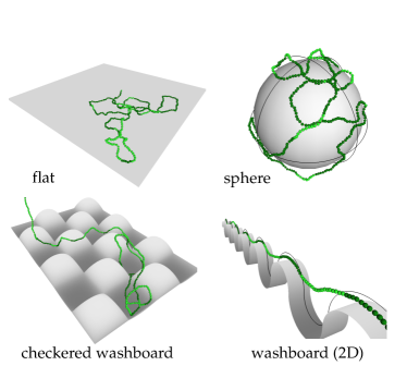
Figure 1: Schematic figure of adsorption geometries studied in this paper. The darker beads are adsorbed onto the surface.

The spherical adsorption geometry is relevant for complexation of DNA or other polyelectrolytes with oppositely charged colloids or histone proteins Wallin and Linse (1996); Kong and Muthukumar (1998); Netz and Joanny (1999b); Schiessel et al. (2000); Kunze and Netz (2000); Cherstvy and Winkler (2011). In Refs. 36 and 38, a minimum of the critical charge for a wrapping transition has been found as a function of the electrostatic screening length using numerical minimization of bending and electrostatic energies. Here, we include thermal fluctuations in the adsorption problem. Based on the results for the planar geometry we can make analytical estimates for a spherical adsorber, which also exhibit a local minimum in the critical potential strength for adsorption as a function of the potential range due to a crossover from thermally driven to bending energy driven desorption. These results are in quantitative agreement with our Monte-Carlo simulations for this geometry.

Structured adsorbing substrates can give rise to interesting shape transitions of semiflexible polymers in the adsorbed state Hochrein et al. (2007); Gutjahr, Lipowsky, and Kierfeld (2010) and also give rise to activated dynamics of polymers Kraikivski, Lipowsky, and Kierfeld (2004, 2005). Here, we focus on the influence of the surface structure on the adsorption transition itself for a washboard and checkered washboard geometry. Adsorption of semiflexible polymers on washboard structures has been considered analytically in Ref. 45. Using scaling arguments and Monte-Carlo simulations, we find a single adsorption transition for a washboard surface structure with a critical adsorption strength, which exhibits a rich behavior as a function of polymer stiffness: Whereas we have a single local maximum in the critical adsorption strength as a function of polymer stiffness for a planar substrate, we find two maxima and one local minimum for a washboard surface structure. For a checkered washboard surface structure the local minimum is suppressed again and we find a single maximum, which is broadened as compared to a planar substrate. We identify the range of persistence lengths, for which the adsorption threshold can be effectively changed and, thus, controlled by the substrate curvature.

The paper is organized as follows. In the next section, we introduce the theoretical and simulation model for semiflexible polymers, and the Monte-Carlo simulation technique. The paper is then divided into two parts. First, we study the adsorption onto a flat surface. We focus on the critical potential strength and its dependence on polymer rigidity, which is determined analytically by scaling arguments and transfer matrix calculations and numerically from Monte-Carlo simulations. In the second part, we investigate adsorption onto curved substrates for a sphere, a washboard and a checkered washboard surface. Using scaling arguments and Monte-Carlo simulations, we determine the critical potential strength for these surfaces as a function of polymer rigidity. This allows us to predict how adsorption of semiflexible polymers can be controlled by the curvatures of the surface structure. Finally, we relate our results to experiments on polyelectrolyte adsorption.

II Model and Simulation

II.1 Model

The fundamental model to describe freely fluctuating inextensible semiflexible polymers on all length scales is the Kratky-Porod model, also known as worm-like chain model Kratky and Porod (1949); Harris and Hearst (1966). The Hamiltonian for a polymer with contour ${\bf r}(s)$, which is parametrized by the arc length $s$, is given by the bending energy

$$\mathcal{H}_{b}[{{\bf r}}(s)]=\frac{\kappa}{2}\int_{0}^{L}\mathrm{d}s\left(\partial_{s}^{2}{\bf r}(s)\right)^{2},$$ (1)

where $\kappa$ is the bending rigidity and $L$ the contour length of the polymer. The persistence length $L_{p,D}$ of the worm-like chain is defined as the decay length of tangent correlations in $D$ spatial dimensions and is given by Kleinert (2006); Gutjahr, Lipowsky, and Kierfeld (2006)

$$L_{p,D}=\frac{2\kappa}{(D-1)k_{B}T}.$$ (2)

In the following, we will use use $L_{p}$ to denote the three-dimensional persistence length, $L_{p}\equiv L_{p,3}=\kappa/k_{B}T$. The worm-like chain model contains the two limiting cases of flexible polymers for $L_{p}\ll L$ and rod-like polymers for $L_{p}\gg L$.

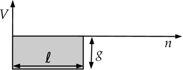
Figure 2: Square-well adsorption potential $V(n)$ as a function of the coordinate $n$ perpendicular to the wall (for a flat substrate $n=z$).

Adsorption by an attractive planar or curved surface is modeled by a potential $V(n)$ per polymer length, which only depends on the coordinate $n$ perpendicular to the surface. The surface is at $n=0$; for a planar surface in the xy-plane, the coordinate $n$ is the Cartesian coordinate $z$. The adsorption potential consists of a short-ranged attractive square-well potential $V_{a}(n)$ of potential range $\ell$ and with an energy gain $g>0$ per unit length of an adsorbed polymer and a hard wall potential $V_{\rm wall}(n)$, see Fig. 2,

$$V(n)=V_{a}(n)+V_{\rm wall}(n)=\begin{cases}\infty&\mbox{ for }n<0\\ -g&\mbox{ for }0<n\leq\ell\\ 0&\mbox{ for }n>\ell.\end{cases}$$ (3)

The total adsorption energy is $\mathcal{H}_{ad}[{{\bf r}}(s)]=\int_{0}^{L}\mathrm{d}s\,V(n(s))$. Short-range attractive potentials can arise from van der Waals forces or screened electrostatic interactions. In these cases, the potential range $\ell$ is comparable to the polymer thickness or the Debye-Hückel screening length, respectively. For polyelectrolytes, we have $g/k_{B}T\sim\sigma\tau l_{B}/\tilde{\kappa}$ and $\ell\sim\tilde{\kappa}^{-1}$, where $l_{B}=e^{2}/4\pi\varepsilon_{0}\varepsilon k_{B}T$ is the Bjerrum length, $1/\sigma$ is the area per unit charge on the surface, $1/\tau$ is the length per unit charge on the polymer and $\tilde{\kappa}=(8\pi l_{B}c)^{1/2}$ is the inverse Debye screening length depending on the total concentration $c$ of (monovalent) counter-ions Netz and Joanny (1999a). The polyelectrolyte persistence length is given by the sum of the bare mechanical persistence length $L_{p,\text{mech}}$ and an electrostatic contribution, $L_{p}=L_{p,\text{mech}}+l_{B}\tau^{2}/4\tilde{\kappa}^{2}$ Odijk (1977); Skolnick and Fixman (1977).

Whereas our findings for the critical potential strength $g_{c}$ for adsorption will depend on microscopic features of the attractive potential such as the potential range, results for critical exponents are expected to apply to all short-ranged interaction potentials, i.e., to all potentials which decay faster than $z^{-2/3}$ for large separations $z$. Lipowsky (1989). We also expect the parameter dependence of the critical potential strength for all short-range adhesion potentials, which have only one characteristic length scale $\ell$ for the potential range and one energy scale $g$ for the potential strength, to be identical to our generic square-well potential. Numerical prefactors can vary. Therefore, our results for the parameter dependence of the critical potential strength for adsorption should also apply, for example, to polyelectrolytes using the above identifications $\ell\sim\tilde{\kappa}$ and $g\sim\sigma\tau l_{B}/\tilde{\kappa}$.

A weakly bent semiflexible polymer without overhangs has a preferred orientation parallel to the adsorbing surface. For a planar surface this allows for a particularly simple Monge parametrization by choosing the $x$-coordinate along the the preferred orientation and ${\bf r}(x)=(x,y(x),z(x))$, which leads to

$$\mathcal{H}[z(x)]=\mathcal{H}_{b}[z(x)]+\mathcal{H}_{ad}[z(x)]$$

$$\approx\int_{0}^{L}\mathrm{d}x\,\frac{\kappa}{2}(\partial^{2}_{x}z)^{2}+\int_{0}^{L}\mathrm{d}x\,V_{a}(z(x))$$ (4)

where we used $ds=dx(1+(\partial_{x}y)^{2}+(\partial_{x}z)^{2})^{1/2}\approx dx$ assuming weakly bent configurations. Then, fluctuations in $y(x)$ decouple and can be neglected for the planar adsorption problem, which can be treated as a two-dimensional problem of configurations $(x,z(x))$ in a plane as done in eq. (4). We use the Hamiltonian (4) for analytical transfer matrix calculations for adsorption on planar substrates.

For a free polymer, the assumption of weak bending is valid as long as $\langle(\partial_{x}z)^{2}\rangle,\langle(\partial_{x}y)^{2}\rangle\sim L/L_{p}\ll 1$, i.e., for contour lengths below the persistence length. At the adsorption transition, the correlation length $\xi$ of the transition is an additional relevant length scale, which is comparable to the typical length of unbound polymer segments (so-called loops). For an adsorbed polymer, the weak bending approximation remains valid as long as the contour length of these unbound segments is smaller than the persistence length, $\xi\ll L_{p}$, even if $L\gg L_{p}$.

We neglect effects from self-avoidance. Generally, we expect this to be a good approximation as long as typical polymer configurations are elongated and contain only few loops, as it is the case for sufficiently stiff polymers. We will discuss possible effects of self-avoidance on our results in the end of the paper.

II.2 Simulation model

In order to perform Monte-Carlo simulations we use a discrete and extensible representation of the semiflexible polymer in terms of the semiflexible harmonic chain (SHC) model Kierfeld et al. (2004). The SHC model represents a discretization of the original worm-like chain model (1) with additional bond extensibility and is, therefore, not limited to the weak bending regime. The SHC model consists of a fixed number $N+1$ of beads ${\bf r}_{i}$ ($i=0,...,N$) connected by $N$ bonds ${\bf t}_{i}\equiv{\bf r}_{i+1}-{\bf r}_{i}$ ($i=0,...,N-1$) with equilibrium length $b_{0}$, such that $N=L/b_{0}$. Each bond is extensible with a harmonic stretching energy $(k/2)\left(|{\bf t}_{i}|-b_{0}\right)^{2}$. The SHC Hamiltonian containing the discretized version of the bending energy (1) and the harmonic stretching energies is given by

$$\mathcal{H}_{\rm SHC}=\frac{\kappa}{b_{0}}\sum_{i=1}^{N-2}\left(1-\hat{{\bf t}}_{i}\cdot\hat{{\bf t}}_{i+1}\right)+\frac{kb_{0}^{2}}{2}\sum_{i=0}^{N-1}\left(\frac{|{\bf t}_{i}|}{b_{0}}-1\right)^{2},$$ (5)

where $\hat{{\bf t}}_{i}={{\bf t}_{i}}/{\left|{\bf t}_{i}\right|}$ are the unit tangent vectors. Extensible bonds allow for a more effective Monte-Carlo simulation using displacement moves of the beads. The use of bead displacement moves is preferred over bond rotation moves because the adsorption energy is naturally given in terms of bead positions. The discretized adsorption energy used in the SHC simulations is $\mathcal{H}_{ad}[\{{\bf r_{i}}\}]=\sum_{i=0}^{N-1}b_{0}V(n_{i}(s))$.

In order to approximate an inextensible worm-like chain we have to choose the bond extensibility $k$ as large as possible. Real polymers always have a certain mechanical extensibility. Moreover, the SHC model is a coarse-grained model of a worm-like chain, which does not contain configurational fluctuations on length scales smaller than $b_{0}$. Therefore, an upper bound for $k$ is given by the entropic elasticity associated with the stored filament length within each segment of contour length $b_{0}$. If we use $N=100$ segments in simulations to discretize a polymer of micrometer length, for example an actin filament of contour length $L=10~{}{\rm\mu m}$ the bond length $b=0.1~{}{\rm\mu m}$ is much larger than the actin monomer size and each bond can perform configurational fluctuations reducing its length to an apparent bond length $b$. In response to a tensile force $f$ fluctuations are pulled out, and we find MacKintosh, Käs, and Janmey (1995)

$$b_{0}-b=\frac{b}{\pi}\int_{\pi/b_{0}}^{\infty}\mathclose{\!\mathrm{d}}q\,\frac{k_{B}T}{\kappa q^{2}+f}\approx\frac{b_{0}^{2}}{\pi^{2}L_{p}}+\frac{b_{0}^{4}}{3\pi^{4}k_{B}TL_{p}^{2}}f,$$ (6)

where we only integrate over small wavelength fluctuations with $q>\pi/b_{0}$, which correspond to shape fluctuations of a single segment. If $f\ll\kappa/b^{2}$ the stretching is weak and the expansion in eq. (6) justified. From the last term we obtain the entropic stiffness

$$k=3\pi^{4}k_{B}TL_{p}^{2}/b_{0}^{4}.$$ (7)

For actin filaments, this entropic stiffness is much smaller than the mechanical stiffnessKojima, Ishijima, and Yanagida (1994) and, therefore, dominates the elasticity (entropic and mechanical springs have to be considered loaded in series rather than parallel).

II.3 Adsorption geometries

Apart from adsorption to a planar substrate, we also investigate adsorption to three different curved substrates (shown in Fig. 1) in $D=2$ or $D=3$ spatial dimensions: (i) adsorption to a sphere of radius $R_{s}$ in $D=3$ dimensions, (ii) adsorption to a washboard surface consisting of a sequence of alternating concave and convex half-circles of radius $R_{w}$ in $D=2$ dimensions. (iii) adsorption to a checkered washboard potential consisting of a square lattice of alternating concave and convex spherical pieces of radius $R_{c}$ in $D=3$ dimensions.

For all three geometries we focus on the critical potential strength $g_{c}$ as a function of polymer stiffness, which is captured by the dimensionless ratio $L_{p}/\ell$ of persistence length and potential range.

II.4 Simulation

We perform extensive Monte-Carlo (MC) simulations of the adsorption process for all four geometries. We use the Metropolis algorithm with bead displacement moves of single beads or segments of beads as shown in Fig. 3. We always attach one end of the polymer to the boundary of the attractive potential, i.e., at $n=\ell$, in order to suppress diffusive motion of the polymer center of mass in the desorbed phase.

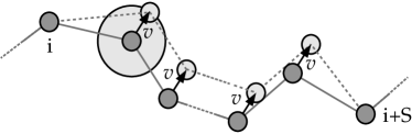
Figure 3: MC moves used in the simulation. Each move displaces segments of $S$ successive beads, but the bending and stretching energy for only two tangents at the ends of the segment have to be updated. The choice of the distribution of $S$ depends on the simulated geometry; large values of $S$ are only suitable for free polymers. A single monomer displacement corresponds to the special case $S=1$.

In the simulation we measure lengths in units of the bond length $b_{0}$ and energies in units of $k_{B}T$. Typical simulated polymers consist of several hundreds of beads. The number of beads $N$ is at least $200$ to minimize finite size effects. Each MC sweep consists of $N$ MC moves, where segments of $S$ successive beads are moved by a random vector of length $v$. The MC displacement $v$ is determined before each simulation to realize an acceptance rate of about $50\%$ (typical values are $v\simeq 0.05$). A typical MC simulation consists of $10^{7}$ sweeps. The entropic spring constant $k\sim 300\,k_{B}TL_{p}^{2}/b_{0}^{4}$ (see eq. (7)) is very high due to the large prefactor and the quadratic dependence on the persistence length. We use smaller values such as $k=100\,k_{B}T/b_{0}^{2}$ or $k=1000\,k_{B}T/b_{0}^{2}$, which are also independent of $L_{p}$, to speed up the simulation, because the displacement length $v$ is determined by the dominant energy and has to be chosen very small for stiff springs $k$.

It turns out that the most important control parameter for the adsorption transitions is the ratio $L_{p}/\ell$. The parameter ranges that we explore are $0.5\leq\ell/b_{0}\leq 10$ and $1\leq L_{p}/b_{0}\leq 10000$, i.e., $10^{-1}\leq L_{p}/\ell\leq 10^{4}$. We only consider persistence lengths larger than one bond length, $L_{p}>b_{0}$. For smaller persistence lengths $L_{p}<b_{0}$, effects from the stiffness are always negligible as compared to discretization effects and the effective persistence length will be $L_{p}\sim b_{0}$ such that lowering $L_{p}$ below $b_{0}$ would not further decrease the effective stiffness.

For simulations with curved surfaces, the curvature can be characterized by a curvature radius $R$. For typical applications, curvature radii larger than the potential range $\ell$ should be most interesting. Therefore we focus on this parameter regime. We also choose $R$ larger than $b_{0}$, otherwise discretization effects dominate curvature effects.

III Adsorption to a planar substrate

III.1 Analytical results

The parameter dependence of the critical potential strength for adsorption to a planar substrate can be obtained from a simple scaling argument, which takes into account the competition between the entropic free energy cost of confining an adsorbed polymer to the attractive region $0<z<\ell$ of the square-well potential and the the adsorption energy gain. The entropic free energy cost can be estimated by the deflection length $\lambda$, which is the typical length scale between contacts with the confining boundaries Odijk (1983). The resulting free energy cost per length is approximately $1k_{B}T$ per deflection length Maggs, Huse, and Leibler (1989); Gompper and Seifert (1990). The adsorption energy gain per length is $-g$. Therefore the total free energy change per length upon adsorption is $\Delta f=k_{B}T/\lambda-g$. Adsorption requires $\Delta f<0$ or $g>g_{c}$ with a critical potential strength of the form $g_{c}\sim{k_{B}T}/{\lambda}$.

For a semiflexible polymer with $L_{p}\gg\ell$, the collision condition $\langle z^{2}\rangle(\lambda)\sim\lambda^{3}/L_{p}=\ell^{2}$ for a thermally fluctuating segment of contour length $\lambda$ gives Odijk (1983); Köster et al. (2007); Köster, Kierfeld, and Pfohl (2008) $\lambda_{SF}\sim L_{p}^{1/3}\ell^{2/3}\gg L_{p}$. The resulting critical potential strength for adsorption is Gompper and Seifert (1990); Kierfeld and Lipowsky (2003)

$$g_{c}\sim\frac{k_{B}T}{\lambda_{SF}}=c_{SF}\frac{k_{B}T}{\ell}\left(\frac{L_{p}}{\ell}\right)^{-1/3}.$$ (8)

This parameter dependence of $g_{c}$ has been obtained previously in Refs. 26; 30; 31 and in the context of polyelectrolytes in Ref. 20. In Ref. 32, adsorption by discrete linker molecules instead of a continuous adsorption potential has been considered by transfer matrix methods taking the thermodynamic limit of an infinite linker number per length. The results of Ref. 32 can only be compared to the other approaches if the polymer length $L_{m}$ between linkers becomes small; they lead to the same parameter dependence (8) only if the linker distance $L_{m}$ is identified with the deflection length of the adsorption potential (i.e., setting $J\sim gL_{m}$ and $L_{m}\sim\lambda_{SF}$ in Ref. 32).

Here, we use transfer matrix methods to go beyond the parameter dependence (8) and also derive the analytical result

$$c_{SF}=3^{-1/3}\Gamma(1/3)/2\simeq 0.929$$ (9)

for the numerical prefactor in Supplementsup (IC) for a square-well potential in the limit $\ell\ll L_{p}$. In this limit, the adsorbed semiflexible polymer is sufficiently stiff that coiling within the potential range $\ell$ is suppressed and $\langle z^{2}\rangle(\lambda)\sim\lambda^{3}/L_{p}$ holds.

For $L_{p}\ll\ell$, on the other hand, such coiling occurs, and we have to employ a flexible polymer model with a Kuhn length $b_{K}=2L_{p,D}$ in order to describe the adsorption transition. For such a flexible polymer segment of length $\lambda$, we have $\langle z^{2}\rangle(\lambda)\sim\lambda b_{k}\sim\lambda L_{p}$ and collisions with the confining boundary happen on a deflection length scale $\lambda_{F}\sim\ell^{2}/L_{p}\ll L_{p}$ as obtained from the collision condition $\langle z^{2}\rangle(\lambda_{F})\sim\ell^{2}$. Adsorption then requires a critical potential strength

$$g_{c}\sim\frac{k_{B}T}{\lambda_{F}}=c_{F}\frac{k_{B}T}{\ell}\frac{L_{p}}{\ell}.$$ (10)

Using standard transfer matrix methods for flexible polymers and solving the equivalent problem of a quantum mechanical particle in a square-well potential de Gennes (1979), one finds $c_{F}=2\pi^{2}/4D(D-1)$ for the numerical prefactor in $D$ dimensions.

Remarkably, the results (8) for a semiflexible polymer with $L_{p}\gg\ell$ and (10) for a flexible polymer with $L_{p}\ll\ell$ show a rather different behavior as a function of polymer stiffness $L_{p}$: whereas the critical adsorption potential strength $g_{c}$ is increasing with stiffness in the flexible regime, it decreases with stiffness in the stiff regime. Both in the stiff and in the flexible limit the critical potential strength for adsorption becomes small. The driving force behind this behavior is, however, different. In the stiff limit, the entropic free energy cost for adsorption becomes small because for a stiff polymer shape fluctuations are small, and the stiff polymer does not lose much configurational entropy upon adsorption. In the flexible limit, on the other hand, the effective monomer length decreases (and the effective monomer number increases) with stiffness. For a small monomer size, positional fluctuations and, thus, the entropy cost of confinement also decrease. Therefore, also in the flexible limit the configurational entropy cost during adsorption becomes small. As a result, we expect a maximum of the critical potential strength for adsorption in the intermediate stiffness regime, where $L_{p}\sim\ell$. Hence, adsorption is most difficult if polymer persistence length and adsorption potential range are tuned to match each other. This has interesting consequences for applications because tuning the polymer rigidity such that the persistence length $L_{p}$ matches the potential range $\ell$ could be a measure to prevent adsorption.

In order to quantify the location of the maximum, we will use an interpolating function $I(x)$ describing the critical adsorption potential as a function of the dimensionless stiffness parameter $L_{p}/\ell$,

$$\frac{g_{c}\ell}{k_{B}T}=I\left(\frac{L_{p}}{\ell}\right),$$ (11)

which captures the correct asymptotics in the semiflexible and flexible limit,

$$I(x) \approx c_{F}x~{}~{}\mbox{for}~{}~{}x\ll 1$$ (12)

$$I(x) \approx c_{SF}x^{-1/3}~{}~{}\mbox{for}~{}~{}x\gg 1$$ (13)

according to (8) and (10). Furthermore, in the stiff limit, the leading corrections from flexibility are of the order

$$I(x)\approx c_{SF}x^{-1/3}+{\mathcal{O}}(x^{-1}),$$ (14)

see Ref. 15 and the discussion in Supplementsup (IC3). An interpolation function $I(x)$ has to fulfill the three constraints (12), (13), and (14). We will obtain a fourth constraint below.

An interpolating scaling function $I(x)$ can be motivated by the behavior in the stiff limit (13). Additional compatibility with the flexible limit (12) suggests $I(x)=c_{1}x/(1+c_{2}x^{4/3})^{-1}$ with $c_{1}=c_{F}$ and $c_{2}=c_{F}/c_{SF}$. The constraint (14) on the next to leading order term in the stiff limit then suggests the presence of another term,

$$I(x)=c_{1}x(1+c_{2}x^{4/3}+c_{3}x^{2/3})^{-1}.$$ (15)

This scaling function contains three free fit parameters $c_{1}$, $c_{2}$, and $c_{3}$. The choices $c_{1}=c_{F}$ and $c_{2}=c_{F}/c_{SF}$ will reproduce the known flexible and semiflexible limits (12) and (13), respectively, and the remaining parameter $c_{3}$ allows to vary the position of the maximum.

A scaling function similar to eq. (15) has also been used to describe numerical transfer matrix calculations in Ref. 34. The interpolation function of Deng et al. differs in two aspects: (i) the numerical prefactor $c_{SF}$, see eq. (13), has been treated as a completely free fit parameter because an analytical result was not available, and (ii) the interpolation function does not obey the constraint (14) because of a next to leading term in the stiff limit $I_{\text{Deng}}(x)\approx c_{SF}x^{-1/3}+\mathcal{O}(x^{-4/3})$. A more detailed discussion of this scaling function is given in Supplementsup (IA).

Alternatively, we can use the above scaling argument for the deflection length $\lambda$ and $g_{c}\sim k_{B}T/\lambda$ to motivate an alternative functional form of the interpolation function $I(x)$ with only two free fit parameters, which is described in Supplementsup (IB). The derivation in Supplementsup (IB) also suggests as a fourth constraint, that the interpolation function $I(x)$ should obey the functional form

$$I(x)\sim\frac{x^{-1/3}}{\tilde{g}({\rm const}\,x^{-2/3})}~{}~{}\mbox{for}~{}x\gg 1$$ (16)

in the stiff limit, where $\tilde{g}(x)$ is an analytical function $\tilde{g}(x)$ with $\tilde{g}(0)\neq 0$. The interpolation function (15) as well as the alternative interpolation function given in the Supplementsup fulfill this constraint, whereas the scaling function used in Ref. 34 does not obey this constraint.

III.2 Numerical results

We determine the critical potential strength from the MC simulations using two different methods: (i) by order parameter cumulants and (ii) finite size scaling. Finite size scaling (ii) also allows us to determine the free energy exponent $\nu$. The simulation results for the critical potential strength are summarized in the phase diagrams Fig. 4(A) for $D=3$ and Fig. 4(B) for $D=2$. The resulting fit parameters $c_{1}$, $c_{2}$, and $c_{3}$ for the interpolation function $I(x)$ from eq.  (15) are shown in Table 1.

III.2.1 Critical potential strength via third order parameter cumulant

An effective method to determine the critical potential strength uses the fact that the derivative of the free energy density with respect to the potential strength $g$ gives the mean fraction of polymer length in the square-well potential, which provides an order parameter for the adsorption transition. Derivatives of the free energy with respect to $g$ generate cumulants of the mean fraction of adsorbed polymer length. In the Supplementsup (IIA) we discuss in detail that the second cumulant is expected to have a maximum at the transition and, thus, the third cumulant a zero. We use this criterion both for the planar and for curved geometries to locate the adsorption transition.

The simulation results for the critical potential strength $g_{c}$ as determined by the third cumulant are summarized in the phase diagrams Fig. 4(A) for $D=3$ and Fig. 4(B) for $D=2$ (circles). The resulting fit parameters of the interpolation functions from eqs.  (15) and (S3) from Supplementsup (IB) are shown in Table 1.

In the stiff limit, we find good agreement with the analytical result (8) as can also be seen from the values for the fit parameter combination $c_{2}c_{SF}/c_{1}$ of the interpolating function $I(x)$ from eq.  (15) in Table 1, which are close to our analytial result $c_{2}c_{SF}/c_{1}=1$ in the stiff limit. In the flexible limit, simulation results for $g_{c}$ are slightly larger than the analytical result (10) in $D=3$ and smaller in $D=2$ as can be seen from the values for the fit parameter $c_{1}$ of the interpolating function in Table 1: we expect $c_{1}/c_{F}=1$ from the analytical results in the flexible limit and find $c_{1}/c_{F}\gtrsim 1$ for $D=3$ and $c_{1}/c_{F}\lesssim 1$ for $D=2$. One reason for this deviation is the finite size of the polymer; simulation results tend to the analytical result (10) with increasing length of the polymer (using the same discretization $b_{0}$). We also examine discretization effects by changing the bond length $b_{0}\rightarrow ab_{0}$ by a factor $a$ and accordingly $N\rightarrow{N}/{a}$ to keep the polymer length $L=Na$ constant. This allows further to explore smaller values for $L_{p}/\ell$, without violating the condition $L_{p}>b_{0}$, which ensures that the persistence length is not cut off by the discretization $b_{0}$. The simulation data in Fig.  4 shows that changing the discretization $b_{0}$ has only little effect on the critical potential strength.

For $D=2$ we also show simulation snapshots of typical polymer configurations in Fig. 5. These snapshots are taken in the adsorbed phase close to the critical potential strength. We can clearly distinguish the different characteristics of configurations in the the stiff and flexible limit, which give rise to the different adsorption behavior: in the flexible limit $L_{p}/\ell<1$, the adsorbed polymer exhibits turns within the attractive potential layer of width $\ell$ giving rise to compact adsorbed configurations. In the stiff limit $L_{p}/\ell>1$, on the other hand, the configurations are elongated without turns within the attractive potential layer.

A comparison of our numerical results for $D=2$ and $D=3$ (see Fig. 4 (A) and (B)) shows that the critical adsorption strength is indeed independent of the number of transversal dimensions in the stiff limit in agreement with eq. (8) and (9). This justifies our treatment with only one transversal dimension within the Monge approximation see eq. (4). Also the asymptote in the flexible limit is independent of dimensionality except for the prefactor in agreement with eq. (10). Therefore, the general shape of the critical potential strength as a function of stiffness with maximum for $L_{p}\sim\ell$ is valid for all dimensions.

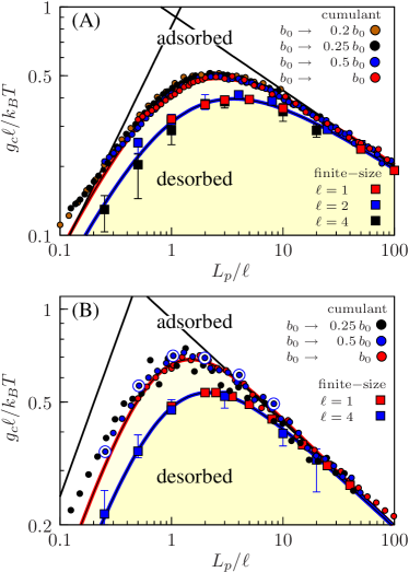
Figure 4: Phase diagram for a flat substrate in (A) $D=3$ and (B) $D=2$ as obtained from MC simulations. The double logarithmic plot shows the dimensionless critical potential strength $g_{c}\ell/k_{B}T$ as a function of the dimensionless stiffness parameter $L_{p}/\ell$ with increasing bending stiffness from left to right. The yellow region marks the desorbed state. The analytical results (8) in the stiff limit and (10) in the flexible limit are shown as straight black lines. Circles show results for the critical potential strength as determined from the zero of the third order parameter cumulant using simulation parameters $N=200$, $\ell=2b_{0}$, and $k=1000\,k_{B}T/b_{0}^{2}$. By changing $b_{0}$ we check that the discretization length $b_{0}$ has no influence on our results. Squares show results from finite size scaling for $k=1000\,k_{B}T/b_{0}^{2}$. The colored curves show interpolation function (15) with fit parameters $c_{1}$, $c_{2}$, and $c_{3}$ as given in Table 1 for the cumulant method (red curves) and the finite size method (blue curves). Large blue circles in (B) correspond to the simulation snapshots shown in Fig. 5.

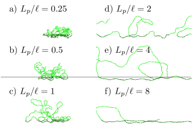
Figure 5: Typical simulation configurations for adsorption on a flat substrate in $D=2$ for increasing stiffness parameters $L_{p}/\ell$. Snapshots are taken in the adsorbed phase close to the critical potential strength. The simulation parameters are $N=400$, $\ell=4b_{0}$, and $k=250\,k_{B}T/b_{0}^{2}$.

data set	$c_{1}/c_{F}$	$c_{2}c_{SF}/c_{1}$	$c_{3}$	$\text{max}(I)$
theory (D=3)	$1$	$1$	free
cumulant	$1.13{\pm}0.05$	$1.03{\pm}0.01$	$0.26{\pm}0.06$	$2.61$
finite size	$0.9{\pm}0.1$	$1.01{\pm}0.03$	$0.6{\pm}0.2$	$3.60$
theory (D=2)	1	$1$	free
cumulant	$0.51{\pm}0.03$	$0.97{\pm}0.01$	${-}0.48{\pm}0.05$	$1.49$
finite size	$0.40{\pm}0.01$	$0.98{\pm}0.01$	${-}0.03{\pm}0.04$	$2.13$

Table 1: Simulation results for the fit parameters $c_{1}$, $c_{2}$, and $c_{3}$ for the interpolation function $I(x)$ from eq.  (15) in comparison with theoretical expectations. The maximum value of the resulting interpolation function is given for comparison. All fits for the cumulant method are performed for MC data from simulations with $N=200$, $\ell=2b_{0}$, $k=1000\,k_{B}T/b_{0}^{2}$. For the analysis of simulation data we use the cumulant method or finite size scaling as explained in the text.

III.2.2 Critical exponent and potential strength via finite size scaling

We also use finite size scaling of the specific heat to corroborate our results for the critical potential strength and to calculate the critical exponent $\nu$ for the correlation length and the free energy. The (extensive) specific heat $C=\beta^{2}\left(\left\langle\mathcal{H}^{2}\right\rangle-\left\langle\mathcal{H}\right\rangle^{2}\right)$ exhibits finite size scaling according to

$$L^{-{2}/{\nu}}\beta^{2}\left(\left\langle\mathcal{H}^{2}\right\rangle-\left\langle\mathcal{H}\right\rangle^{2}\right)=f\left((g-g_{c})L^{{1}/{\nu}}\right)$$ (17)

with a scaling function $f(x)$. This expression is rather natural for a continuous transition, but it is important to note that it also applies if the adsorption transition is of first order, where Binder (1987)

$$L^{-2}\beta^{2}\left(\left\langle\mathcal{H}^{2}\right\rangle-\left\langle\mathcal{H}\right\rangle^{2}\right)=f_{1}\left((g-g_{c})L^{d}\right)$$ (18)

with a scaling function $f_{1}(x)$ and $d$ as the internal dimension of the system. This expression is actually of the same form as expression (17) for a continuous transition because a polymer has internal dimension $d=1$, and we have $\nu=1$ for a first order transition. Therefore, there is no systematic bias regarding the order of the transition if eq. (17) is used for finite size scaling. In Supplementsup (IIB), we explain in detail how the best parameter set $(\nu,\,g_{c})$ for the finite size scaling (17) is determined using a systematic error minimization procedure.

Data for the critical potential strength $g_{c}$ as obtained from the finite size scaling procedure is presented in the phase diagrams 4 (A) and 4 (B) (squares). We find good agreement with our analytical result. The resulting fit parameters of the interpolation functions from eqs.  (15) and (S3) from Supplementsup (IB) are shown in Table 1.

The finite size scaling procedure also allows us to determine the critical exponent $\nu$. As discussed in Supplementsup (III), we find an exponent $\nu$ around $\nu=2$ for small bending rigidity, which lowers towards $\nu=1$ with increasing stiffness. This is in agreement with the theoretical expectation that a semiflexible polymer should exhibit a critical behavior corresponding to $\nu_{SF}=1$ with a crossover to a flexible behavior with $\nu=\nu_{F}=2$ in the small regime $|g-g_{c,SF}|<k_{B}T/L_{p}$ around the transition, where the correlation length $\xi$ exceeds $L_{p}$.

IV Adsorption to curved substrates

Because semiflexible polymers have a bending rigidity, adsorption can be controlled by an additional curvature of the adsorbing surface. We investigate the influence of surface curvature for three different geometries, an adsorbing sphere, an adsorbing washboard and a checkered washboard surface as shown in Fig.  1 both in $D=2$ and $D=3$ spatial dimensions.

Depending on the polymer stiffness several additional effects can occur for adsorption on curved substrates: (i) Flexible polymers with $L_{p}<\ell$ adsorb in a compact conformation on a flat substrate, as can be seen in Fig. 4a). Concave curvatures with radii $R>\ell$ can give rise to an increased adhesion energy gain because the polymer can realize a larger contact area with the adhesive potential, see Fig. 7a). This effect favors adsorption on a curved substrate and is relevant for washboard potentials. (ii) For stiff polymers with $L_{p}>\ell$ an additional bending energy cost occurs during adsorption on a curved substrate. This effect favors desorption and is the most relevant effect to effectively control the adsorption for all geometries we consider by tuning the substrate curvature radius $R$.

IV.1 Adsorption to a sphere

An additional bending energy cost arises for adsorption of a stiff semiflexible polymer with $L_{p}>\ell$ to a sphere with radius $R_{s}$. For a polymer of length $L$ firmly adsorbed with curvature $1/R_{s}$ the additional total bending energy is $E_{R}\sim\frac{1}{2}L\kappa/R_{s}^{2}$. We can include this energy into the simple scaling argument for the critical potential strength. The total free energy change per length upon adsorption becomes $\Delta f=k_{B}T/\lambda-g+k_{B}TL_{p}/2R_{s}^{2}$ with the deflection length $\lambda\sim L_{p}^{1/3}\ell^{2/3}$, which we assume to be unchanged by curvature effects (which should be justified for $R_{s}\gg\lambda$ Köster, Kierfeld, and Pfohl (2008)). The adsorption condition $\Delta f<0$ leads to the following estimate for the critical potential strength,

$$\frac{g_{c}\ell}{k_{B}T}=g_{c}(R_{s}=\infty)+\frac{L_{p}\ell}{2R_{s}^{2}}=c_{SF}\left(\frac{L_{p}}{\ell}\right)^{-1/3}+\frac{L_{p}\ell}{2R_{s}^{2}}$$ (19)

with the critical potential strength $g_{c}(R_{s}=\infty)$ for a planar substrate from eq. (8).

The result (19) can also be interpreted in terms of the contact curvature radius $R_{co}\sim(\kappa/|\Delta f|)^{1/2}$ for polymer adsorption by an effective contact potential of strengthKierfeld (2006) $\Delta f=k_{B}T/\lambda-g$, which is given by the free energy of adsorption to a planar substrate. The adsorption condition $g>g_{c}$ with $g_{c}$ as given by (19) corresponds to the condition $R_{co}<R_{s}$ that the contact curvature is smaller than the sphere radius.

MC simulation data agree well with the analytical result (19) for the adsorption threshold. We describe our MC simulation results for the critical potential strength (as obtained by the cumulant method) by eq.  (19) with the radius $R_{s}$ as fit parameter. We expect the resulting effective adsorption radius to be of the order $R_{s}+\ell/2$. The simulation results are shown in the phase diagram in Fig. 6 and exhibit good agreement with eq. (19) with effective curvature radii within the interval $[R_{s},R_{s}+\ell]$. In Fig. 6 we also show the reduced critical potential strength $g_{c}\ell/k_{B}T-{L_{p}\ell}/{2R_{s}^{2}}$, which agrees very well with our results for a planar substrate.

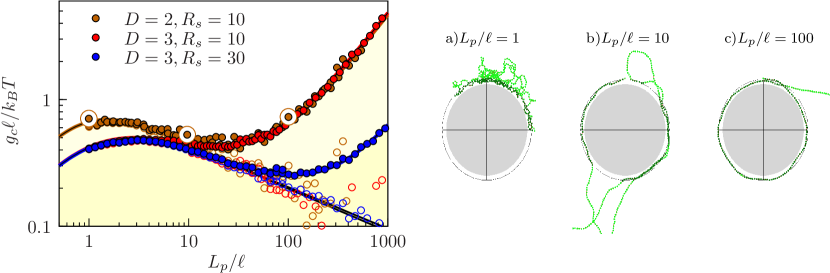
Figure 6: Left: Phase diagram for an adhesive sphere in $D=3$ and $D=2$ as obtained from MC simulations: double logarithmic plot of the dimensionless critical potential strength $g_{c}\ell/k_{B}T$ as a function of the dimensionless stiffness parameter $L_{p}/\ell$ as obtained with the cumulant method. Simulation parameters are $N=200$, $\ell=b_{0}$, and $k=1000\,k_{B}T/b_{0}^{2}$. Equation (19) is used to fit the data via an effective sphere radius $R_{s}$; the results are $R_{s,1}/\ell=10.46{\pm}0.06$, $R_{s,2}/\ell=10.27{\pm}0.02$ and $R_{s,3}/\ell=30.6{\pm}0.2$. Filled circles are original MC results, hollow circles show the reduced potential strength $g_{c}\ell/k_{B}T-{L_{p}\ell}/{2R_{s}^{2}}$, which agrees well with our simulation results for a planar surface. Right: Typical simulation configurations for increasing stiffness parameters $L_{p}/\ell$ and $R_{s}=10\ell$. Snapshots are taken in the adsorbed phase close to the critical potential strength. The simulation parameters are $N=400$, $\ell=2b_{0}$, and $k=100\,k_{B}T/b_{0}^{2}$. The simulation snapshots correspond to the large brown circles in the phase diagram on the left.

Remarkably, the critical potential strength (19) has a local minimum at

$$\frac{L_{p}}{\ell}\sim\left(\frac{R_{s}}{\ell}\right)^{3/2}$$ (20)

with $g_{c,\text{min}}\sim({k_{B}T}/{\ell})\left({\ell}/{R_{s}}\right)^{1/2}$ because of the bending energy correction. This can be used to design an “optimally sticky” sphere for adsorption of a semiflexible polymer by choosing a radius $R_{s,opt}\sim\ell(L_{p}/\ell)^{2/3}$ for given persistence length and potential range or by choosing an optimal potential range $\ell_{opt}\sim R_{s}^{3}/L_{p}^{2}$ for given sphere radius and persistence length. The latter can be realized for polyelectrolytes by adjusting the salt concentration. In the absence of thermal fluctuations, such a minimum in the critical potential strength for adsorption has also been found for the complexation of polyelectrolytes with oppositely charges spheres Netz and Joanny (1999b); Kunze and Netz (2000).

IV.2 Washboard surface

In $D=3$ dimensions the washboard surface is translationally invariant in one direction and is composed of alternating half-cylinders of radius $R_{w}$, see Fig. 1. Then the polymer orients parallel to the half-cylinders during adsorption in order to avoid additional bending energies, and the critical potential strength for adsorption is very similar to the planar surface result. Consequently, the substrate structure radius $R_{w}$ gives no control on the adsorption threshold for a cylindrical washboard in $D=3$.

Therefore, we focus first on washboard surfaces in $D=2$ dimensions, which are composed of half-circles of radius $R_{w}$. This two-dimensional adsorption geometry is equivalent to the situation where the polymer is confined to a two-dimensional plane perpendicular to the half-cylinders of a three-dimensional washboard surface. We will show that under this confinement, pronounced effects from the surface structure occur, and the substrate curvature radius can be used to control adsorption. Afterwards, we will discuss the checkered washboard surface as an alternative substrate structure to effectively control the adsorption threshold in $D=3$ spatial dimensions without applying additional constraints.

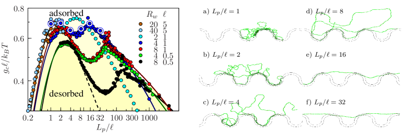
Figure 7: Left: Phase diagram for an adhesive washboard surface in $D=2$ as obtained from MC simulations: double logarithmic plot of the dimensionless critical potential strength $g_{c}\ell/k_{B}T$ as a function of the dimensionless stiffness parameter $L_{p}/\ell$ as obtained with the cumulant method for different values $R_{w}/\ell=2,4,8,16$. The remaining simulation parameters are $N=200$, and $k=100\,k_{B}T/b_{0}^{2}$. The solid lines show fits using eq. (8) (using $R_{s}$ as fit parameter) for an adsorbing sphere for small $L_{p}/\ell$ and fits using eq.  (25) (using $w_{1}$ and $w_{2}$ as fit parameters) for larger stiffnesses $L_{p}/\ell$. The dashed line is the fit for the flat substrate. Right: Typical simulation configurations for increasing stiffness parameters $L_{p}/\ell$ and $R_{w}=4\ell$. Snapshots are taken in the adsorbed phase close to the critical potential strength. The simulation parameters are $N=400$, $\ell=2b_{0}$, and $k=100\,k_{B}T/b_{0}^{2}$. The simulation snapshots correspond to the large blue circles in the phase diagram on the left.

Fig. 7 shows typical simulation snapshots and the phase diagram for the adsorption transition on a washboard surface in $D=2$. The simulation snapshots illustrate the following four distinct regimes of characteristic adsorption behavior:

• $R_{w}\gg L_{p}\approx\ell$: The concavely curved valleys of the washboard surface support adsorption of a flexible polymer in a compact shape.

• $R_{w}>L_{p}>\ell$: The curvature is negligible on the scale of the persistence length. We find adsorption to an effectively planar substrate in an elongated shape.

• $R_{w}\approx L_{p}\gg\ell$: The scale of the persistence length corresponds to a single half-sphere. The adsorption behavior is similar to adsorption on a single sphere.

• $L_{p}>R_{w}\gg\ell$: The persistence length is larger than a half-sphere radius. This results in “incomplete” adsorption on the tips of the washboard substrate.

For $L_{p}\lesssim R_{w}$ (snapshots a)-d)), we have a “complete” adsorption into the concavely curved valleys of the washboard structure. Because there is only one such valley on the scale of the persistence length, the adsorption threshold for “complete” adsorption is well described by the previous result (19) for adsorption to a single sphere, where we use $R_{s}=R_{w}$.

This result is only modified in the regime of “incomplete” adsorption on top of the washboard surface for stiff polymers with $L_{p}>R_{w}$. In this regime, bound configurations consist of an alternating sequence of short adhered segments on top of the half-spheres and free segments of (projected) length $4R_{w}$ between adhered segments. To estimate the critical potential strength we calculate the free energy difference of such an incompletely adsorbed configuration to the completely unbound state.

The free segments between the adsorption points have a partition sum $Z(4R_{w})\sim Z_{0}(4R_{w})\ell\alpha L_{p}/(4R_{w})^{2}$. where $Z_{0}(4R_{w})$ is the unconstrained partition sum of the free polymer and $Z(4R_{w})$ the partition sum constrained to hit the top of the half-circle within a distance $\ell$ and with a tangentGompper and Burkhardt (1989); Benetatos and Frey (2003) $v\leq\alpha$. The scaling $z^{2}\sim L^{3}/L_{p}$ and $v^{2}\sim L/L_{p}=(z/L_{p})^{2/3}$ implies $\alpha\sim(\ell/L_{p})^{1/3}$. This results in an entropic free energy loss per length of

$$\Delta f_{\rm free} =-w_{1}\frac{k_{B}T}{4R_{w}}\ln(Z(4R_{w})/Z_{0}(4R_{w}))$$

$$=w_{1}\frac{k_{B}T}{4R_{w}}\ln\left[w_{2}\frac{16R_{w}^{2}}{L_{p}\ell}\left(\frac{L_{p}}{\ell}\right)^{1/3}\right]$$ (21)

with two numerical constants $w_{1}$ and $w_{2}$. Each short adhered segment of length $\Delta L$ on top of the half-circle within the attractive layer of thickness $\ell$ contributes a free energy difference $\Delta f\Delta L=(-g+k_{B}T/\lambda_{SF})\Delta L$ comparable to a segment adsorbed on planar substrate. Because there is one segment per length $4R_{w}$ between adhered segments the resulting free energy difference per length is given by

$$\Delta f_{\rm ad} =\frac{\Delta L}{4R_{w}}\left(-g+c_{SF}\frac{k_{B}T}{\ell^{2/3}L_{p}^{1/3}}\right)$$ (22)

The condition $\Delta f_{\rm free}+\Delta f_{\rm ad}<0$ for adsorption results in a critical potential strength

$$g_{c}=c_{SF}\frac{k_{B}T}{\ell^{2/3}L_{p}^{1/3}}+w_{1}\frac{k_{B}T}{\Delta L}\ln\left[16w_{2}\left(\frac{R_{w}}{\ell}\right)^{2}\left(\frac{\ell}{L_{p}}\right)^{2/3}\right]$$ (23)

For straight polymers ($T=0$, $L_{p}\gg R_{w}$), the length $\Delta L$ is calculated from the geometrical relation $R_{w}^{2}+\Delta L^{2}=(R_{w}+\ell)^{2}$, which gives $\Delta L=2\sqrt{R_{w}\ell}\left(1+{\cal O}(\ell/R_{w})\right)$. In the presence of thermal fluctuations the polymer can use an energy $k_{B}T$ to adapt further to the potential and increase the adsorbed length $\Delta L$. Equating the thermal angular fluctuations $\Delta\alpha=(\Delta L/L_{p})^{1/2}$ over a length $\Delta L$ with the curvature angle $\alpha=\Delta L/R_{w}$ of the half-circle, we obtain $\Delta L={R_{w}^{2}}/{L_{p}}$. Both effects should add up to give $\Delta L=2\sqrt{R_{w}\ell}+{R_{w}^{2}}/{L_{p}}$. The first contribution dominates for larger stiffnesses

$$\frac{L_{p}}{\ell}\gg\left(\frac{R_{w}}{\ell}\right)^{3/2}.$$ (24)

For these stiffnesses we can also neglect the first entropic contribution in the result (23) for the critical adsorption strength in eq. (23) and find

$$\frac{g_{c}\ell}{k_{B}T} =w_{1}\frac{1}{2\sqrt{R_{w}/\ell}}\ln\left[16w_{2}\left(\frac{R_{w}}{\ell}\right)^{2}\left(\frac{\ell}{L_{p}}\right)^{2/3}\right]$$ (25)

which is only logarithmically $L_{p}$-dependent.

For smaller stiffness $(L_{p}/\ell)\ll(R/\ell)^{3/2}$ we find

$$\frac{g_{c}\ell}{k_{B}T} =c_{SF}\left(\frac{L_{p}}{\ell}\right)^{-1/3}$$

$$~{}~{}+w_{1}\frac{L_{p}\ell}{R_{w}^{2}}\ln\left[16w_{2}\left(\frac{R_{w}}{\ell}\right)^{2}\left(\frac{\ell}{L_{p}}\right)^{2/3}\right]$$ (26)

which is very similar to the complete adsorption result as given by the single sphere result (19) with $R_{s}=R_{w}$. The crossover from complete to incomplete adsorption should happen if the condition (24) is fulfilled. Therefore, incomplete adsorption on top of the washboard only involves short straight segments $\Delta L\sim 2\sqrt{R\ell}$ without much curvature in agreement with the simulation snapshots e) and f) in Fig. 7.

Incomplete adsorption is different from the adsorption transitions discussed in Refs. 59; 45, where it has been proposed that adsorption proceeds via the shortening of desorbed bridges between segments strongly adsorbed in the concave valleys of the washboard surface. The main differences in Refs. 59; 45 are (i) the use of a contact adsorption potential in Refs. 59; 45, which corresponds to the limit $\ell\approx 0$, (ii) the presence of a tension, which is absent in our system, as we do not consider external stretching forces and (iii) a surface undulation amplitude, which is small compared to the wavelength, where we consider a washboard structure consisting of half-circles, i.e., the undulation amplitude equals the wavelength. For a contact potential, incomplete adsorption on top of the substrate has for zero temperature only been found in the presence of tension in Ref. 59. A finite potential range $\ell>0$ as used in the present work favors incomplete adsorption because it gives rise to a length $\Delta L>0$ of adsorbed segments an, thus, an extensive adhesion energy for a straight rod, i.e., in the limit of infinite stiffness. For a contact potential, on the other hand, a straight rod touches the adhesive structure only at single points an the adhesion energy is zero. Furthermore a finite potential range allows for thermal fluctuations within the potential at non-zero temperatures, also favoring a (incompletely) adsorbed phase.

The MC simulation results in the phase diagram in Fig. 7 show good agreement with the analytical result (25) for the adsorption threshold in the regime of incomplete adsorption for stiff polymers fulfilling (24). We can successfully fit the MC data for the critical potential strength (as obtained using the cumulant method) using eq. (25) with the numerical constants $w_{1}$ and $w_{2}$ as fit parameters. The resulting values for the leading order fit parameter $w_{1}$ (see Table 2) are indeed independent of the substrate curvature radius $R_{w}/\ell$.

$R_{w}/b_{0}$	$\ell/b_{0}$	$R_{s}/\ell$	$w_{1}$	$w_{2}$
$4$	$1$	$4.6{{\pm}}0.1$	$0.532{{\pm}}0.005$	$4.5{{\pm}}0.2$
$8$	$1$	$8.29{{\pm}}0.09$	$0.509{{\pm}}0.008$	$7.5{{\pm}}0.7$
$4$	$0.5$	$8.78{{\pm}}0.07$	$0.512{{\pm}}0.006$	$5.9{{\pm}}0.4$
$8$	$0.5$	$15.7{{\pm}}0.1$	$0.47{{\pm}}0.02$	$11{{\pm}}3$

Table 2: Simulation results for the fit parameters $R_{s}$, $w_{1}$ and $w_{2}$ for the interpolation functions (19) for smaller and (25) for larger stiffnesses.

For more flexible polymers violating (24), fits with the result (8) for an adsorbing sphere with $R_{s}$ as fit parameter work well. All resulting values for the effective curvature radii lie in the interval $[R_{w},R_{w}+\ell]$ as expected.

MC simulations and our analytical results for the adsorption threshold show that adsorption control by the substrate curvature radius $R_{w}$ is most efficient in the regime

$$\frac{L_{p}}{\ell}\sim\left(\frac{R_{w}}{\ell}\right)^{3/2}$$ (27)

where the critical potential strength exhibits a local minimum as for adsorption on a single sphere. If the stiffness is increased such that (24) holds, we find incomplete adsorption, where the dependence of $g_{c}$ on the curvature radius $R_{w}$ is much weaker according to eq. (25). This is also clearly supported by the MC simulation results in the phase diagram Fig. 7. If the stiffness is much smaller than the minimum value (27) curvature effects become negligible on the scale of the persistence length, and we find the crossover to effectively planar adsorption. The MC phase diagram in Fig. 7 clearly indicates a window of stiffnesses for adsorption control around the local minimum and in between two local maxima of the critical potential strength. The maximum at small stiffness is located at $L_{p}/\ell\sim 1$ as for planar adsorption, the maximum for large stiffnesses at $L_{p}/\ell\sim({R_{w}}/{\ell})^{3/2}$ as given by the condition (24) for the crossover between complete and incomplete adsorption. The stiffness window for adsorption control vanishes if the substrate curvature radius $R_{w}$ approaches the potential range $\ell$, as can be seen in the phase diagram Fig. 7 (cyan data points for ${R_{w}}/{\ell}=2$).

Our results not only apply to the control of the adsorption of polymers on washboard surfaces, for example, to control polyelectrolyte adsorption by tuning the salt concentration and, thus, the range $\ell$ of the adsorption potential. Another technologically important application is the control of adsorption of graphene sheets to adhesive washboard potentials consisting of a sequence of alternating concave and convex half-cylinders. Our results apply to this problem as well, and a transition from incomplete to complete adsorption has also been discussed for graphene sheets Li and Zhang (2010).

IV.3 Checkered washboard surface

Now we want to discuss washboard substrates in $D=3$ spatial dimensions, which is the relevant case for applications. We propose the checkered washboard (see Fig.  1) as a substrate, which allows to effectively control adsorption by substrate curvature for $D=3$. As pointed out above, a washboard substrate consisting of cylinders (see Fig.  1) does not allow for an adsorption control as the polymer can reorient parallel to the cylinders. To construct a washboard structure in three spatial dimensions where the polymer cannot simply reorient to avoid curvature during adsorption, we consider a checkered washboard consisting of rectangular subunits described by a Cartesian product of two washboard half-circles with a height function $z_{R_{c}}(x,y)={\pm}R_{c}\sqrt{1-(x/R_{c})^{2}}\sqrt{1-(y/R_{c})^{2}}$ ($x,y\in[{-}R_{c},R_{c}]$) with a radius $R_{c}$. These rectangular subunits differ from half-spheres but exhibit the same curvature at the tips of the surface. We expect adsorption on the checkered washboard for $L_{p}\lesssim R_{c}$ to be similar to adsorption to the $D=2$ washboard surface for $L_{p}\lesssim R_{w}$ because there is only a single valley or top on the scale of the persistence length. We expect adsorption to be well described by the result (19) for adsorption to a single sphere, where we use $R_{s}=R_{c}$. For $L_{p}>R_{c}$, however, the alternating checkered structure of valleys and top will modify the adsorption behavior.

In the simulation, we need an effective approximate method to implement the attractive range: For the checkered washboard structure we do not determine the normal distances $n$ from eq. (3) exactly, but approximate the attractive region via $z_{R_{c}}<z<z_{R_{c}+\ell}$. The relative error is worst at the corners and can be estimated as $\frac{1}{\ell}(z_{R_{c}+\ell}-z_{R_{c}})-1\approx 0.155$ for $\ell\ll R_{c}$. The checkered substrate and the numerically determined error for the attractive range is illustrated in 8.

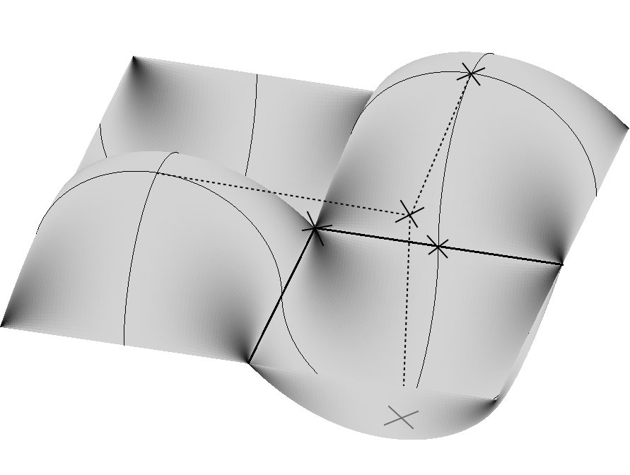
Figure 8: The checkered washboard substrate. Brightness codes for the error in the potential range implementation (see text). Dark color indicates larger errors. Crosses indicate different attachment points of the polymer used in simulations. Thick black lines indicate the square lattice of lines of preferential adsorption.

The MC simulation results in the phase diagram Fig. 9 show that the adsorption threshold can be controlled by the substrate curvature radius $R_{c}$ in a similar fashion as for the washboard substrate in $D=2$ dimensions for $L_{p}\lesssim R_{c}$. However, we find two characteristic differences for stiffer polymers $L_{p}>R_{c}$: (i) As opposed to the $D=2$ washboard substrate we do not find a local minimum of the critical potential strength but we find a single broad maximum or shoulder in the regime ${L_{p}}/{\ell}\sim\left({R_{c}}/{\ell}\right)^{3/2}$ for $R_{c}/\ell\lesssim 10b_{0}$. (ii) The critical potential strength exhibits a remarkably stronger dependence on the substrate curvature radius $R_{c}$ for larger polymer stiffness as compared to the $D=2$ washboard. For large stiffnesses $L_{p}\gg R_{c}$ the critical potential decreases with increasing $R_{c}$ as can be seen in the phase diagram Fig. 9.

In order to illustrate the different adsorption mechanism underlying these characteristic differences we also present typical simulation snapshots in Fig. 9. Whereas we find “incomplete” adsorption on the substrate tips for the washboard substrate in $D=2$ (see simulation snapshots 7 e),f)) for large stiffnesses, the polymer preferentially adsorbs “between” the tops and valleys, i.e., along the straight boundaries of the square subunits for a checkered washboard in the regime of large stiffnesses $L_{p}\gg R_{c}$ as illustrated by the simulation snapshot Fig. 9 c). These boundaries are the equal height lines $z(x,y)=0$ and form a plane-filling square lattice of lines for preferential adsorption with in-plane lattice constant $2R_{c}$, see thick black lines in Fig. 8). No out-of-plane curvature is required for adsorption onto this lattice of straight lines. The regions around each straight line segment is almost vertically tilted but locally flat such that for each adsorbing segment our results for adsorption on a flat substrate will apply. In order to connect between neighboring straight lines of the square lattice of adsorption sites, a stiff polymer has to run through the discrete square lattice of intersection points where four subunits meet.

This restricts the thermal fluctuations of the adsorbed polymer parallel to the surface and implies an additional entropy cost during adsorption because in-plane configurations are restricted. This additional entropy cost can be used to control the adsorption via the distance $2R_{c}$ between the lattice points. This entropy cost can be estimated in an analogous manner as the entropy cost for adsorption on the discrete array of tips for the $D=2$ washboard. Adapting the corresponding estimate (21) for the entropic free energy cost appropriately, we obtain $\Delta f_{\rm ch}=a_{1}({k_{B}T}/{2R_{c}})\ln\left[a_{2}({4R_{c}^{2}}/{L_{p}\ell})\left({L_{p}}/{\ell}\right)^{1/3}\right]$. The additional free energy cost leads to a corresponding shift of the critical potential strength for adsorption as compared to a flat substrate, $g_{c}=g_{c}(R_{s}=\infty)+\Delta f_{\rm ch}$, or

$$\frac{g_{c}\ell}{k_{B}T} =c_{SF}\left(\frac{L_{p}}{\ell}\right)^{-1/3}$$

$$~{}~{}~{}+a_{1}\frac{\ell}{2R_{c}}\ln\left[4a_{2}\left(\frac{R_{c}}{\ell}\right)^{2}\left(\frac{\ell}{L_{p}}\right)^{2/3}\right].$$ (28)

This result predicts an offset in the critical potential strength, which increases for smaller substrate curvature radii $R_{c}$. It depends only logarithmically on the polymer stiffness $L_{p}$. The result (28) exhibits a different dependence of the critical potential strength on the substrate curvature radius $R_{c}$ for larger polymer stiffness as compared to the result (25) for the $D=2$ washboard.

The MC simulation results in the phase diagram in Fig. 9 confirm both of these predictions qualitatively. We can successfully fit the MC data for the critical potential strength (as obtained using the cumulant method) in the stiff regime $L_{p}\gg R_{c}$ using eq. (28) with the numerical constants $a_{1}$ and $a_{2}$ as fit parameters, see Table 3. The fit parameters are indeed roughly independent of the substrate curvature radius $R_{c}/\ell$.

$R_{c}/b_{0}$	$\ell/b_{0}$	$a_{1}$	$a_{2}$
$5$	$1$	$0.25{\pm}0.01$	$73{\pm}15$
$10$	$1$	$0.38{\pm}0.04$	$16{\pm}10$
$20$	$1$	$0.42{\pm}0.04$	$12{\pm}7$
$10$	$0.5$	$0.46{\pm}0.05$	$10{\pm}7$
$20$	$0.5$	$0.42{\pm}0.10$	$24{\pm}43$

Table 3: Simulation results for the fit parameters $a_{1}$ and $a_{2}$ for larger stiffness. We use eq. (28) as fit function.

The MC simulations and the scaling argument for the adsorption threshold show that, using a checkered washboard structure, adsorption can be controlled rather effectively by the substrate curvature radius $R_{c}$ in the entire stiff limit, where $L_{p}\gg R_{c}$. As opposed to the washboard substrate in $D=2$ discussed in the previous section, where a window of stiffnesses for effective adsorption control emerged, adsorption control by a checkered washboard in $D=3$ is still effective for large polymer stiffnesses.

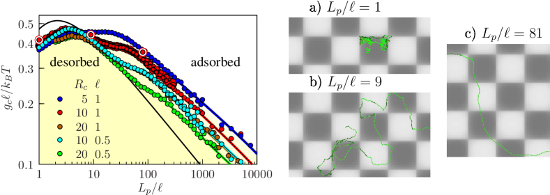
Figure 9: Left: Phase diagram for a checkered substrate as obtained from MC simulations: double logarithmic plot of the dimensionless critical potential strength $g_{c}\ell/k_{B}T$ as a function of the dimensionless stiffness parameter $L_{p}/\ell$ as obtained with the cumulant method. The solid lines show fits using eq.  (28) (using $a_{1}$ and $a_{2}$ as fit parameters) for larger stiffnesses $L_{p}/\ell$. Simulation parameters are $N=200$ and $k=100\,k_{B}T/b_{0}^{2}$. The red data points for $R_{c}/\ell=10$ are results for four different attachment points as shown in Fig. 8. Right: Typical simulation configurations for adsorption on a checkered washboard for increasing stiffness parameters $L_{p}/\ell$. Snapshots are taken in the adsorbed phase close to the critical potential strength. The simulation snapshots correspond to the large red circles in the phase diagram on the left.

V Discussion of experimental results

Many experimental results are available for polyelectrolyte adsorption or complexation. For polyelectrolyte adsorption the potential strength $g/k_{B}T\sim\sigma\tau l_{B}/\tilde{\kappa}$ can be controlled by the surface charge $\sigma$. Experimentally, the critical surface charge $\sigma_{c}$ for polyelectrolyte adsorption can be measured as a function of the inverse Debye screening length $\tilde{\kappa}=(8\pi l_{B}c)^{1/2}$, which is controlled by the salt concentration, resulting in a relationZhang, Ohbu, and Dubin (2000); Cooper et al. (2006) $\sigma_{c}\propto\kappa^{a}$ with a characteristic exponent $a$. Using our results for adsorption to a planar surface, $g_{c}\ell/k_{B}T\sim(L_{p}/\ell)^{-1/3}$ in the stiff regime, see eq. (8) and $g_{c}\ell/k_{B}T\sim L_{p}/\ell$ in the flexible regime, see eq. (10), and using a potential range $\ell\sim 1/\tilde{\kappa}$ given by the Debye screening length, we find

$$\sigma_{c} \propto{\tilde{\kappa}}^{2}(L_{p}/\ell)^{-1/3}~{}(\mbox{stiff}),$$

$$\sigma_{c} \propto{\tilde{\kappa}}^{2}(L_{p}/\ell)~{}(\mbox{flexible}).$$ (29)

According to Odijk Odijk (1977), Fixman and Skolnick Skolnick and Fixman (1977) the polyelectrolyte persistence length is given by the sum of the bare mechanical persistence length $L_{p,\text{mech}}$ and an electrostatic contribution due to the electrostatic self-repulsion of the polymer, $L_{p}=L_{p,\text{mech}}+l_{B}\tau^{2}/4\tilde{\kappa}^{2}$. For a mechanically dominated persistence length we have $L_{p}/\ell\propto\tilde{\kappa}$, whereas we have $L_{p}/\ell\propto\tilde{\kappa}^{-1}$ for an electrostatically dominated persistence length. Combining this with (29), we obtain four possible scaling behaviors $\sigma_{c}\propto\kappa^{a}$ with exponents

$$a =5/3~{}~{}\mbox{mechanical stiffness, stiff limit}$$

$$a =3~{}~{}\mbox{mechanical stiffness, flexible limit}$$

$$a =7/3~{}~{}\mbox{electrostatic stiffness, stiff limit}$$

$$a =1~{}~{}\mbox{electrostatic stiffness, flexible limit},$$

which characterize polyelectrolyte adsorption onto planar surfaces. For curved surfaces such as a sphere, there are additional corrections in the stiff limit according to eq. (19), such that $\sigma_{c}\propto\tilde{\kappa}^{0}(L_{p}/\ell)$, which leads to $\sigma_{c}\propto\tilde{\kappa}$ ($a=1$) for mechanical stiffness and $\sigma_{c}\propto\tilde{\kappa}^{-1}$ ($a=-1$) for electrostatic stiffness.

The experimental results on polyelectrolyte adsorption onto proteins and micelles in Ref. 62 agree best with an exponent $a=1$ corresponding an electrostatic stiffness and the flexible limit for a planar substrate, which is reasonable in view of the short mechanical persistence lengths of the studied polyelectrolytes and with protein radii larger than these persistence lengths.

VI Conclusion

We studied adsorption of semiflexible polymers on planar and curved substrates. Using extensive Monte-Carlo simulations and analytical arguments we showed that the interplay between three characteristic length scales – (i) the persistence length $L_{p}$ characterizing polymer stiffness, (ii) the range $\ell$ of the attractive adsorption potential, and (iii) a characteristic curvature radius $R$ of the surface structure – allows to control the adsorption threshold for semiflexible polymers effectively.

For a planar adsorbing surface we find a maximum of the critical potential strength for adsorption, i.e., a “minimally sticky” surface if the persistence length matches the potential range, $L_{p}\sim\ell$. We presented two scaling functions which can quantitatively describe the crossover between flexible and stiff limit and the location of the maximum in the critical potential strength in agreement with MC simulations, see Fig. 4. We also quantified the exact asymptotic value of the critical potential strength for adsorption in the stiff limit, see eqs. (8) and (9). Our results can also resolve contradictory statements in the literature. Simulations of adsorbing semiflexible polymers in Refs. 18; 19 found a critical potential strength decreasing with stiffness: these simulations probed the stiff limit with a persistence length exceeding the potential range. On the other hand, simulations of adsorbing polyelectrolytes found a critical potential strength increasing with electrostatic stiffness Kong and Muthukumar (1998): these simulations probed the flexible limit with a small electrostatic persistence length.

For an adsorbing sphere of radius $R_{s}$ the critical potential strength is increased for large persistence lengths by the additional bending energy involved in adsorption to a curved object. This results in an “optimally sticky” adsorbing sphere if the condition (20), $L_{p}/\ell\sim(R_{s}/\ell)^{3/2}$ holds. MC simulation results in Fig. 6 confirm this result.

For a washboard surface consisting of cylinders, adsorption control is not possible because the polymer can orient parallel to the cylinders and avoid additional bending during adsorption. The situation is different if we restrict the polymer to a two-dimensional plane perpendicular to the cylinders. For such a washboard surface in two spatial dimension, we find an additional crossover from complete adsorption to an incomplete adsorption on the tips of the surface structure for large persistence lengths. The condition $L_{p}/\ell\gg(R_{w}/\ell)^{3/2}$, see eq. (24), characterizes the regime of incomplete adsorption. The adsorption threshold can be controlled by the substrate curvature in a polymer stiffness window given by $1\lesssim L_{p}/\ell\lesssim({R_{w}}/{\ell})^{3/2}$, as also shown by MC simulations, see Fig. 7 with an “optimally sticky” curvature radius for $L_{p}/\ell\sim(R_{w}/\ell)^{3/2}$, see eq. (27).

Checkered washboard structures offer a possibility to control adsorption also in three spatial dimensions. On the one hand, the checkered washboard suppresses polymer reorientation as for a cylindrical three-dimensional washboard. On the other hand, it suppresses an incomplete adsorption on the tips of the substrate as it occurs for the two-dimensional washboard. For a checkered washboard, stiff polymers rather adsorb in the locally flat straight boundaries between tops and valleys of the structure, which form a square lattice. The driving force for adsorption control on this type of substrate is the restriction to the square array of straight adsorption lines within the adsorbing plane rather than the control of the out-of-plane curvature. As a result, there is no polymer stiffness window for adsorption control, adsorption control always effective for large stiffnesses $L_{p}\gg R_{c}$.

We expect similar results for other, eventually more irregularly curved substrates, where the substrate curvatures can be adjusted to the polymer persistence length and the potential range to create sticky or non-sticky regions. Our results for the washboard surfaces demonstrate that not only the out-of-plane curvature will be important but also the shape and curvature of locally flat preferred lines of adsorption sites, which are given by the lines of equal substrate height.

In this work, we neglected all effects from self-avoidance. Generally, we expect this to be a good approximation as long as typical polymer configurations are elongated and contain only few loops, as it is the case for sufficiently stiff polymers. For the adsorption of semiflexible polymers this is typically the case in the stiff regime $L_{p}/\ell>1$. However, we expect pronounced corrections in the flexible limit $L_{p}/\ell<1$. On the other hand, it is well-known de Gennes (1979) that the critical potential strength adsorption of a self-avoiding chain on a planar substrate is $g_{c}\sim k_{B}T(L_{p}/\ell)^{5/3}$ rather than $g_{c}\sim k_{B}T(L_{p}/\ell)$ in the absence of self-avoidance (see eq. (10)). Therefore, the critical potential remains an increasing function of polymer stiffness. Consequently, we expect the most important features of the phase diagrams, such as the maximum of the critical potential strength as a function of polymer stiffness for adsorption on a planar substrates, to be similar also in the presence of self-avoidance. This remains to be investigated quantitatively in future work.

Supplemental Material for “Controlling adsorption of semiflexible polymers on planar and curved substrates”

The supplemental material is structured as follows: (i) Discussion of different interpolation functions $I(x)$. (ii) Analytical transfer matrix calculation for planar substrate in the stiff limit, which gives the critical potential strength for a square-well potential in the limit of small potential range. (iii) Details of the cumulant method and finite size scaling procedure used to obtain the critical potential strength in Monte-Carlo simulations. (iv) Results for the critical correlation length exponent $\nu$ of the adsorption transition for a planar substrate. (v) Additional simulation snapshots in the desorbed state.

I Adsorption to a planar substrate

I.1 Interpolation function of Deng et al.

In Ref. 1, Deng et al. also use an interpolation function to describe the crossover of the critical potential strength $g_{c}$ for adsorption between the stiff and flexible limit. They measure the critical potential strength in units of $k_{B}T/2L_{p}$ rather than $k_{B}T/\ell$ as in (11); the critical potential strength does not exhibit a maximum if measured in these units. In Ref. 1, an interpolation $g_{c}(2L_{p}/k_{B}T)=\tilde{I}(2L_{p}/\ell)$ with a scaling function

$$\tilde{I}_{\rm Deng}(x)=\frac{(c_{F}/2)x^{2}}{[C_{2}x^{2}+C_{1}x+1]^{2/3}}$$

is used with two fit parameters $C_{1}\simeq 0.94$ and $C_{2}\simeq 0.38$, which are determined from numerical transfer matrix calculations.

Comparing the two scaling forms, we find the relation

$$\tilde{I}(x)=xI(x/2)~{},~{}~{}I(x)=\tilde{I}(2x)/2x$$

Consequently the scaling function proposed in Ref. 1 corresponds to

$$I_{\rm Deng}(x) =\frac{c_{F}x}{[4C_{2}x^{2}+2C_{1}x+1]^{2/3}}$$ (S1)

This scaling function does not obey the constraints (13) and (14) listed in the main text:

• The numerical prefactor $c_{SF}$ has been treated as a fit parameter because an analytical result was not available. Using their fit results, we find $c_{SF}=2^{-4/3}c_{F}C_{2}^{-2/3}\simeq 0.619$, which is close but smaller than our analytical result $c_{SF}\simeq 0.929$. The reason is a different determination of the critical potential strength from simulations. Deng et al.  use an extrapolation of adsorbed fraction, which is the first cumulant of the adsorption energy, to zero, whereas we mainly use the third cumulant.

• The constraint (14) regarding the correct next to leading order asymptotics in the stiff limit has not been applied. The scaling function (S1) has the asymptotics $I_{\rm Deng}(x)=(c_{F}/2C_{2}^{2/3})x^{-1/3}+{\cal O}(x^{-4/3})$ for $x\gg 1$, which differs from the analytical prediction (14).

I.2 Alternative interpolation function $I(x)$.

In this appendix, we use the scaling argument for the deflection length $\lambda$ and $g_{c}\sim k_{B}T/\lambda$ to motivate a functional form of the interpolation function $I(x)$. The argument is based on a result for the thermal displacement $\langle z^{2}\rangle(L)\equiv\langle(z(L)-z(0))^{2}\rangle$ of a free worm-like chain in the direction perpendicular to the average preferred orientation in $x$-direction.

For a free worm-like chain in two dimensions ($D=2$), the thermal displacement $\langle z^{2}\rangle(L)$ can be calculated analytically. In $D=2$, we can parametrize the configuration by a single angle $\theta(s)$ by ${\bf t}(s)=\partial_{s}{\bf r}(s)=(\cos\theta(s),\sin\theta(s))$. The angular correlations are

$$\langle(\theta(s)-\theta(s^{\prime}))^{2}\rangle =\frac{k_{B}T}{\kappa}|s-s^{\prime}|=\frac{2|s-s^{\prime}|}{L_{p,D}}$$

and

$$\langle\theta(s)^{2}\rangle =d_{1}L/L_{p,D}$$

with a numerical constant $d_{1}$. The angular correlations can be used to calculate

$$\langle(z(L){-}z(0))^{2}\rangle=\int_{0}^{L}\!\!\!\!ds_{1}\int_{0}^{L}\!\!\!\!ds_{2}\langle\sin\theta(s_{1})\sin\theta(s_{2})\rangle$$

$$~{}=\int_{0}^{L}ds_{1}\int_{0}^{L}ds_{2}\frac{1}{2}\left(e^{-\frac{1}{2}\langle(\theta(s_{1})-\theta(s_{2}))^{2}\rangle}-e^{-\frac{1}{2}\langle(\theta(s_{1})+\theta(s_{2}))^{2}\rangle}\right)$$

$$~{}=\int_{0}^{L}ds_{1}\int_{0}^{L}ds_{2}\frac{1}{2}\left(e^{-\frac{1}{2}\langle(\theta(s_{1})-\theta(s_{2}))^{2}\rangle}-e^{-\langle\theta^{2}(s_{1})\rangle-\langle\theta^{2}(s_{2})\rangle+\frac{1}{2}\langle(\theta(s_{1})-\theta(s_{2}))^{2}\rangle}\right)$$

$$~{}=\int_{0}^{L}ds_{1}\int_{0}^{s_{1}}ds_{2}\left(e^{-(s_{1}-s_{2})/L_{p,D}}-e^{-2d_{1}L/L_{p,D}}e^{(s_{1}-s_{2})/L_{p,D}}\right)$$

$$~{}=L_{p,D}^{2}\left(\frac{L}{L_{p,D}}-1+e^{-L/L_{p,D}}\right)-e^{-2d_{1}L/L_{p,D}}L_{p,D}^{2}\left(-\frac{L}{L_{p,D}}-1+e^{L/L_{p,D}}\right)$$

$$~{}\equiv L_{p,D}^{2}f_{d_{1}}(L/L_{p,D})$$

Although this calculation is difficult to adapt to three spatial dimensions, we expect a similar behavior for $D=3$ with an eventually different numerical prefactor $d_{2}$:

$$\frac{\langle z^{2}\rangle(L)}{L_{p,D}^{2}}=d_{2}f_{d_{1}}(L/L_{p,D}).$$ (S2)

Because of ${\langle z^{2}\rangle(L)}=\langle({\bf r}(L)-{\bf r}(0))^{2}\rangle/D$ for a free worm-like chain in the flexible limit $L\gg L_{p,D}$, we expect $d_{2}=2/D$. Simulation results for a free SHC in $D=3$, which we present in Fig. S1, confirm the scaling form (S2) with $d_{1}=0.76{\pm}0.08$ and a prefactor $d_{2}=0.61{\pm}0.01$ close to the expectation $d_{2}=2/3$. For the results in $D=2$ we get $d_{2}=0.94{\pm}0.01$, which is close to $d_{2}=1$, and $d_{1}=0.84{\pm}0.09$. Because the scaling form is very insensitive to variation of $d_{2}$ for $L/L_{p,D}\gg 1$, we determine the parameters $d_{1}$ and $d_{2}$ only with values $L/L_{p,D}\leq 10$.

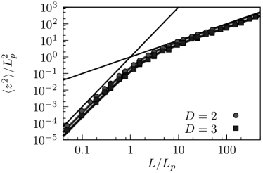
Figure S1: MC data for ${\langle z^{2}\rangle(L)}/{L_{p}^{2}}$ as a function of $L/L_{p}$ for a free worm-like chain in $D=3$ and $D=2$ dimensions confirms the scaling form ${\langle z^{2}\rangle(L)}/{L_{p}^{2}}=cf_{d_{1}}(L/L_{p})$, see eq.  (S2), with $d_{1}=0.76{\pm}0.08$ and a prefactor $d_{2}=0.61{\pm}0.01$ in three and $d_{2}=0.94{\pm}0.01$, $d_{1}=0.84{\pm}0.09$ in two dimensions (for $L/b_{0}=50,100,200,300,400$ and $L_{p}/b_{0}=2,4,8,\ldots,1024$). We fix the first tangent to have a well-defined $z$-direction.

Therefore, the inverse function $f^{-1}_{d_{1}}(x)$ can be used to solve the condition ${\langle z^{2}\rangle(\lambda)}/{L_{p,D}^{2}}=d_{2}f_{d_{1}}(\lambda/L_{p,D})=\ell^{2}/L_{p,D}^{2}$ for the deflection length $\lambda$. This suggests a critical potential strength $g_{c}=(k_{B}T/\ell)I\left(L_{p,D}/\ell\right)$ with a scaling function

$$I(x)=\frac{1}{xf^{-1}_{d_{1}}(x^{-2}/d_{2})}$$ (S3)

with only two free parameters $d_{1}$ and $d_{2}$. In the flexible limit $x=\lambda/L_{p,D}\gg 1$, we use $f_{d_{1}}(x)\approx x$, in the stiff limit $x=\lambda/L_{p,D}\ll 1$, we have $f_{d_{1}}(x)\approx(d_{1}-1/3)x^{3}$. The choices $d_{2}=c_{F}$ and $d_{1}=(c_{SF}/c_{F})^{3}+1/3$ will reproduce the known flexible and stiff limits. In contrast to the interpolation function from eq. (15), the function $I(x)$ in eq. (S3) contains only two free parameters. Therefore, the maximum of interpolation function $I(x)$ is already determined by $d_{1}$ and $d_{2}$.

We have determined the fit parameters $d_{1}$ and $d_{2}$ from the MC simulation results for the critical potential strength both by the cumulant method and finite size scaling and both in $D=2$ and $D=3$. The theoretical expectation $d_{2}/c_{F}=1$ and $\frac{d_{2}}{c^{3}_{SF}}(d_{1}{-}\frac{1}{3})=1$ for the parameters $d_{1}$ and $d_{2}$ agrees reasonably well with the simulation results.

data set	$\frac{d_{2}}{c^{3}_{SF}}(d_{1}{-}\frac{1}{3})$	$d_{2}/c_{F}$	$\text{max}(I)$
theory(D=3)	$1$	$1$	$1.84$
cumulant	$1.21{\pm}0.04$	$0.82{\pm}0.01$	$2.47$
finite size	$1.0{\pm}0.1$	$0.54{\pm}0.02$	$3.36$
theory(D=2)	$1$	$1$	$1.26$
cumulant	$1.5{\pm}0.1$	$0.60{\pm}0.02$	$1.24$
finite size	$1.19{\pm}0.07$	$0.35{\pm}0.01$	$1.92$

Table 4: Simulation results for the fit parameters $d_{1}$ and $d_{2}$ for the interpolation function $I(x)$ from eq. (S3) in comparison with theoretical expectations. The maximum value of the resulting interpolation function is given for comparison. All fits for the cumulant method are performed for MC data from simulations with $N=200$, $\ell=2b_{0}$, $k=1000\,k_{B}T/b_{0}^{2}$. For the analysis of simulation data we use the cumulant method or finite size scaling as explained in the text.

In addition, the scaling argument leading to eq.  (S3) strongly suggests a constraint on the functional form of the scaling function $I(x)$ for the critical potential strength $g_{c}$: The asymptotics for the stiff limit shows that the scaling function $f_{d_{1}}(x)$ has a series expansion $f_{d_{1}}(x)=x^{3}g(x)$ with some analytical function $g(x)$ with $g(0)\neq 0$. Therefore, the inverse function should have a functional form $f_{d_{1}}^{-1}(y)=y^{1/3}\tilde{g}(y^{1/3})$ with another analytical function $\tilde{g}(x)$ with $\tilde{g}(0)\neq 0$. It follows from eq.  (S3) that the scaling function $I(x)$ should have an asymptotic form

$$I(x)\sim\frac{x^{-1/3}}{\tilde{g}({\rm const}\,x^{-2/3})}~{}~{}\mbox{for}~{}x\gg 1.$$ (S4)

Our first choice $I(x)\sim c_{1}x^{-1/3}(c_{2}+c_{3}x^{-2/3}+x^{-4/3})^{-1}$, see eq. (15), also fulfills this constraint, whereas the scaling function used in Ref. 1 does not meet this constraint.

I.3 Analytical transfer matrix calculation in the semiflexible limit

Using the transfer matrix method in the weakly bent or stiff limit $L_{p}\gg\ell$ we will give an analytical derivation of the critical adsorption strength for weakly bent semiflexible polymers for a planar surface and a short-range adsorption potential, i.e., determine the numerical prefactor $c_{SF}$ in (8) analytically.

In the following we measure all length scales in Kuhn lengths $2L_{p}=2\kappa/k_{B}T$ and all energies in $k_{B}T$, i.e., we replace

$$z\to\frac{z}{2L_{p}},~{}\ell\to\frac{\ell}{2L_{p}},~{}L\to\frac{L}{2L_{p}},~{}g\to\frac{2L_{p}}{k_{B}T}g.$$ (S5)

In the stiff limit we have $\ell\ll 1$ in rescaled units. We consider the restricted partition sum $Z(z,v,z_{0},v_{0},L)$ of a semiflexible polymer of length $L$ with initial point $z(0)=z_{0}$, initial tangent $\partial_{x}z(0)=v_{0}$, end point $z(L)=z$, and end tangent $\partial_{x}z(L)=v$ in the Monge representation (4) appropriate for a weakly bent polymer. The restricted partition sum $Z(z,v,z_{0},v_{0},L)$ fulfills a transfer matrix equation of the Klein-Kramers type Freed (1972)

$$\partial_{L}Z=\left(-v\partial_{z}+\partial^{2}_{v}-V(z)\right)Z$$ (S6)

with boundary condition $Z(z,v,z_{0},v_{0},0)=\delta(z-z_{0})\delta(v-v_{0})$ at $L=0$.

For an adsorbed polymer we make the Ansatz $Z(x,v,z_{0},v_{0},L)\sim Z_{E}(z,v)e^{-EL}$ where $E=\Delta f<0$ is the adsorption free energy per length of the polymer, i.e., the free energy difference of the adsorbed state as compared to the free state ($V=0$). We approach the desorption transition for $E\nearrow 0$. The “stationary” restricted partition function $Z_{E}(z,v)$ (which we normalize according to $\int dz\int dvZ_{E}(z,v)Z_{E}(z,-v)=1$) fulfillsMaggs, Huse, and Leibler (1989); Gompper and Burkhardt (1989)

$$-EZ_{E}=\left(-v\partial_{z}+\partial^{2}_{v}-V(z)\right)Z_{E}.$$ (S7)

In general we obtain a complete spectrum of solutions for energy eigenvalues $E_{n}$ with a ground state energy $E_{0}$. The solution $Z(z,v,z_{0},v_{0},L)$ satisfying the boundary conditions at $L=0$ is obtained by summing over all solutions, $Z(z,v,z_{0},v_{0},L)=\sum_{n}Z_{E_{n}}(z,v)Z_{E_{n}}(z_{0},-v_{0})e^{-E_{n}L}$. On length scales $L\gg\xi=1/|E_{0}|$ exceeding the correlation length $\xi$ of the adsorption transition, the ground state dominates and

$$Z(z,v,z_{0},v_{0},L)\approx Z_{E_{0}}(z,v)Z_{E_{0}}(z_{0},-v_{0})e^{-E_{0}L}.$$ (S8)

The ground state partition function $Z_{E_{0}}(z,v)$ contains the information about the segment distribution $c(z,v)\sim Z_{E_{0}}(z,v)Z_{E_{0}}(z,-v)$ of a polymer segment in the adsorbed state. The ground state energy $E_{0}$ determines the free energy of adsorption $\Delta f=E_{0}<0$ and the correlation length of the adsorption transition via $\xi=1/|E_{0}|$. The condition $E_{0}=0$ determines the critical potential strength $g_{c}$ for adsorption. The partition function $Z_{0}(z,v)$ at $E_{0}=0$ gives the critical segment distribution. Our main aim will be to determine $g_{c}$ from the condition $E_{0}=0$ in the following. Scaling properties of $Z_{E_{0}}(z,v)$ and $Z(z,v,z_{0},v_{0},L)$ have already been discussed in Refs. Kierfeld and Lipowsky (2003, 2005).

In order to calculate the ground state energy $E$ (we leave out to subscript “0” in the following) and the corresponding “stationary” restricted partition function $Z_{E}(z,v)$, we first consider the region $z>\ell$ outside the potential range, where $V(z)=0$ and we can separate the $z$-dependence for the adsorbed state using $Z_{E}=e^{-\alpha z}\Psi_{\alpha,E}(v)$, because the operators $\partial_{z}$ and $v\alpha+\partial^{2}_{v}$ commute. The function $\Psi_{\alpha,E}(v)$ satisfies

$$(\alpha v+\partial^{2}_{v})\Psi_{\alpha,E}=-E\Psi_{\alpha,E},$$

(analogous to the Schrödinger equation of a quantum particle in an electric field $\alpha$), which gives

$$\Psi_{\alpha,E}(v)=\alpha^{-1/6}\mathrm{Ai}\left(-\left(v\alpha^{1/3}+E\alpha^{-2/3}\right)\right),$$

where $\mathrm{Ai}\left(x\right)$ is the Airy function Abramowitz and Stegun (1972). The ground state solution for $z>\ell$ has to be a linear combination of the eigenfunctions of $\partial_{z}$ and $\alpha v+\partial^{2}_{v}$

$$Z_{E}(z,v)=\int_{0}^{\infty}\mathclose{\!\mathrm{d}}\alpha\,A_{E}(\alpha)e^{-\alpha z}\Psi_{\alpha,E}(v).$$ (S9)

with a coefficient function $A_{E}(\alpha)$.

The coefficient function has to be determined by a family of matching and boundary conditions at the potential well and the wall, that is at $z=\ell$ and $z=0$. In the limit of a small potential depth we approximate the square-well adsorbing potential $V_{a}(z)$ by a delta-function in the middle of the square-well, $V_{a}/z)=-g\ell\delta(z-\ell/2)$, with the same integrated potential strength $\int_{0}^{\ell}V_{a}(z)=-g\ell$ (shaded area in Fig. 2). This approximation is valid in the stiff limit $\ell\to 0$. Integrating the stationary transfer matrix equation (S7) over $z$ from $0$ to $\ell$ and neglecting the terms of higher order in $\ell$ we get matching conditions

$$v\left(Z_{E}(\ell,v)-Z_{E}(0,v)\right)=g\ell Z_{E}(\ell/2,v)$$ (S10)

for each $v$. We also have to obey boundary conditions $Z_{E}(0,v)=0$ for all $v>0$: It is not possible that the last tangent is starting at the wall at $z=0$ and pointing away ($v>0$) because continuity of tangents would lead to configurations crossing the wall.

I.3.1 Critical potential strength

In order to determine the coefficient function $A_{E}(\tilde{\alpha})$ we make use of a setBurkhardt (1993) of functions $\Phi_{\alpha,E}$, which are biorthogonal to $\Psi_{\alpha,E}(z,v)$

$$\int_{0}^{\infty}\mathclose{\!\mathrm{d}}v\,v\Psi_{\alpha,E}(v)\Phi_{\tilde{\alpha},E}(v)=\delta(\alpha-\tilde{\alpha}).$$ (S11)

on the half-space $v>0$. We use the representation (S9) in the matching condition (S10) and apply $\int_{0}^{\infty}\mathclose{\!\mathrm{d}}v\,...\Phi_{\tilde{\alpha},E}(v)$ on both sides of the matching condition to make use of the biorthogonality (S11). Assuming a small potential width we approximate $\exp(\tilde{\alpha}\ell)\approx 1$ and obtain a self-consistent integral equation for the coefficient function $A_{E}(\tilde{\alpha})$

$$A_{E}(\tilde{\alpha}) =g\ell\int_{0}^{\infty}\mathclose{\!\mathrm{d}}v\,\int_{0}^{\infty}\mathclose{\!\mathrm{d}}\alpha\,A_{E}(\alpha)e^{-\ell\alpha/2}\times$$

$$~{}~{}~{}~{}~{}~{}~{}~{}~{}~{}~{}~{}~{}~{}~{}~{}~{}~{}\Psi_{\alpha,E}(v)\Phi_{\tilde{\alpha},E}(v).$$

Investigating this integral equation for $E\approx 0$ in the vicinity of the adsorption transition will allow us to (i) determine $A_{E}(\alpha)$ and thus the polymer segment distribution and (ii) to find the critical potential strength $g_{c}$ at the transition $E=0$.

We substitute $\alpha={2\beta}/{\ell}$ and $v=w(\ell/2)^{1/3}$, which implies $\Psi_{\alpha,E}(v)=(\ell/2)^{1/6}\Psi_{\beta,E(\ell/2)^{2/3}}(w)$, and obtain

$$A_{E}(\tilde{\alpha}) =g\ell\left(\frac{\ell}{2}\right)^{-\frac{1}{2}}\int_{0}^{\infty}\!\!\mathclose{\!\mathrm{d}}w\,\int_{0}^{\beta}\!\!\mathclose{\!\mathrm{d}}\beta\,e^{-\beta}\times$$

$$\Psi_{\beta,E(\ell/2)^{2/3}}(w)\Phi_{\tilde{\alpha},E}\left(w(\ell/2)^{1/3}\right)A_{E}(2\beta/\ell).$$ (S12)

In principle, this integral equation can be solved by iteration. We start with $A_{E}(\alpha)\approx A_{E}$, which is assumed to be independent of $\alpha$. Iterating this equation once for $E\approx 0$ close to the transition and in the stiff limit $\ell\ll 1$, we find that the resulting first iteration for $A_{E}(\alpha)$ is indeed only weakly dependent on $\alpha$ for $E\approx 0$ and remains independent of $\alpha$ exactly at the transition $E=0$. Therefore, the first iteration already gives the correct scaling behavior of $A_{E}(\alpha)$ and allows to determine the critical potential strength $g_{c}$ exactly for $E=0$. For constant $A_{E}$ and $E(\ell/2)^{2/3}\approx 0$, we can perform the $\beta$-integration to obtain

$$B(w) \equiv\int_{0}^{\beta}\mathclose{\!\mathrm{d}}\beta\,e^{-\beta}\Psi_{\beta,0}(w)$$

$$=2^{1/3}3^{-2/3}\dfrac{\Gamma\left(\frac{1}{2}\right)}{\Gamma\left(\frac{1}{3}\right)}\text{M}_{\frac{5}{6},\frac{2}{3}}\left(-\frac{w^{3}}{9}\right)+$$

$$~{}~{}~{}~{}2^{-4/3}3^{-5/6}\dfrac{\Gamma\left(\frac{1}{3}\right)}{\Gamma\left(\frac{1}{2}\right)}w\text{M}_{\frac{7}{6},\frac{4}{3}}\left(-\frac{w^{3}}{9}\right),$$ (S13)

where $\text{M}_{a,b}(x)$ is Kummer’s confluent hypergeometric function of the first kind Abramowitz and Stegun (1972), and eq.  (S12) becomes

$$A_{E}(\tilde{\alpha}) =g\ell\left(\frac{\ell}{2}\right)^{-1/2}\int_{0}^{\infty}\mathclose{\!\mathrm{d}}w\,B(w)$$

$$~{}~{}~{}\times\Phi_{\tilde{\alpha},E}\left(w(\ell/2)^{1/3}\right)A_{E}$$ (S14)

The $\alpha$-dependence of the coefficient function $A_{E}$ in eq. (S14) stems from the biorthogonal function, and we find

$$A_{E}(\alpha)=\tilde{\cal N}_{E,\ell}\int_{0}^{\infty}\mathclose{\!\mathrm{d}}w\,B(w)\Phi_{\alpha,E}\left(w(\ell/2)^{1/3}\right)$$ (S15)

with a normalization factor $\tilde{\cal N}_{E,\ell}$, which is independent of $\alpha$ but can depend on $E$ and $\ell$ in general.

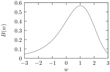
Figure S2: Function $B(w)$, see eq. (S13) with a maximum at $w\simeq 1.01$.

Because $B(w)$ decreases exponentially for $w\gg 1$, see Fig. S2, and $\ell\ll 1$ in the stiff limit, we can use an approximation for small arguments,

$$\Phi_{\alpha,E}\left(w(\ell/2)^{1/3}\right)\approx\frac{\sqrt{3w}}{\pi}\left(\frac{\ell}{2}\right)^{1/6}e^{-\frac{2}{3}{(-E)^{3/2}}/{\alpha}}.$$ (S16)

This leads to

$$A_{E}(\alpha)\approx{\cal N}_{\ell}\exp\left(-\frac{2}{3}\frac{(-E)^{3/2}}{\alpha}\right)$$ (S17)

in the stiff limit $\ell\ll 1$ with a modified normalization factor ${\cal N}_{\ell}$. Using this result for $A_{E}(\alpha)$, we find that the normalization factor ${\cal N}_{\ell}\propto\ell^{-1/3}$ is independent on $E$. The coefficient function $A_{E}(\alpha)$ becomes indeed independent of $\alpha$ for $E\approx 0$, i.e., close to the transition. This justifies our initial assumption of a constant coefficient function $A_{E}(\alpha)\approx A_{E}(0)$. Therefore, the first iteration already provides a self-consistent solution of equation (S12) in the limits of interest.

In order to obtain the critical potential strength $g_{c}$ we set $E=0$ in (S14) and use $\int_{0}^{\infty}\mathclose{\!\mathrm{d}}w\,B(w)w^{1/2}=2^{1/3}3^{-1/6}\pi/\Gamma\left(1/3\right)$ to find

$$\frac{1}{g_{c}\ell} =\frac{\sqrt{3}}{\pi}\left(\frac{\ell}{2}\right)^{-1/3}\left(\int_{0}^{\infty}\mathclose{\!\mathrm{d}}w\,B(w)w^{1/2}\right)$$

$$=\frac{2^{2/3}3^{1/3}}{\Gamma\left(1/3\right)}\ell^{-1/3}$$ (S18)

In original unrescaled units, see eq. (S5), this corresponds to a critical potential strength

$$g_{c}=2^{-1}3^{-1/3}\Gamma\left(1/3\right)\frac{k_{B}T}{\ell}\left(\frac{L_{p}}{\ell}\right)^{-1/3}$$ (S19)

The scaling behavior of $g_{c}$ agrees with the result (8) from the scaling argument and we quantify the numerical prefactor in (8) to be $c_{SF}=2^{-1}3^{-1/3}\Gamma(1/3)\simeq 0.929$.

I.3.2 Critical exponent $\nu$

The exponent $\nu$ characterizes the critical behavior of the ground state energy $|E|\sim|g-g_{c}|^{\nu}$ as a function of $g-g_{c}$ close to the adsorption transition at $E=0$. Because of the relations $|\Delta f|=|E|=1/\xi$, the exponent $\nu$ characterizes both the critical behavior of the correlation length $\xi$ and of the free energy of adsorption $\Delta f$ (i.e., hyperscaling holds). For $g>g_{c}$, the correlation length $\xi$ of the adsorption transition is defined by the distribution of loops lengths, which decays exponentially for large loop lengths with a characteristic decay length given by the correlation length $\xi$.

Because the exponent $\nu$ characterizes the critical free energy behavior, it also determines the order of the adsorption transition: For $\nu>1$ the transition is continuous, whereas it is a first order transition for $\nu<1$. It is a remarkable feature of the polymer adsorption transition that a correlation length $\xi=1/|E|$, which describes the typical length scale of loops, can always be defined and diverges at the transition, even if the transition is of first order.

Using the result (S15) for $A_{E}(\alpha)$ in the self-consistent equation (S12), we obtain the relation $g=g(E)$ in the form

$$\frac{1}{g\ell} \approx\frac{1}{\tilde{\cal N}_{\ell}}\int dvZ_{E}(\ell,v)$$ (S20)

Expanding about $E\approx 0$ gives the exponent $\nu$. A leading $|E|$-dependence $Z_{E}(\ell,v)-Z_{0}(\ell,v)\sim|E|^{3/2}$ has been obtained in Ref. 8 and suggests $\int dv(Z_{E}(\ell,v)-Z_{0}(\ell,v))\sim|E|$, corresponding to $\nu=1$. Thus, the transfer matrix approach in the approximation of a weakly bent semiflexible polymer givesKierfeld and Lipowsky (2003) $\nu=\nu_{SF}=1$ for purely position-dependent adsorption potentials as we use here. This suggests that the adsorption transition is first order or second order with a weak logarithmic correction Kierfeld and Lipowsky (2003, 2005).

I.3.3 Corrections from Crossover to an effective flexible polymer model

The transfer matrix calculation in the approximation of a weakly bent polymer is, strictly speaking, only valid in the stiff limit $L_{p}\to\infty$. Corrections start to arise if the unrescaled correlation length $\xi$ exceeds the persistence length $L_{p}$: Because $\xi$ specifies the typical length of an unbound desorbed loop of the polymer, loops start to loose orientation and to develop overhangs if $\xi>L_{p}$ or $\xi=1/|E|>2$ in rescaled units (S5). This happens for potential strengths close to the critical value $g_{c}=g_{c,SF}=c_{SF}({k_{B}T}/{\ell})({L_{p}}/{\ell})^{-1/3}$ in the semiflexible limit as given by eq. (S19) or eq. (8) in the main text (in unrescaled units), where the correlations length $\xi$ starts to increase and the transfer matrix ground state energy $E$ becomes small according to $|E|\sim|g-g_{c}|^{\nu}$ with $\nu=\nu_{SF}=1$. The condition $|E|<1/2$ corresponds to $|g-g_{c}|<1/2$ (or $|g-g_{c}|<k_{B}T/L_{p}$ in unrescaled units).

Because $g_{c}\sim\ell^{-2/3}$ (or $g_{c}\sim(k_{B}T/L_{p})(L_{p}/\ell)^{2/3}$ in unrescaled units, see eq. (S19)), corrections will always dominate if $\ell\gg 1$ such that $|g-g_{c}|<g_{c}\ll 1/2$ for all $g<g_{c}$. In this regime the weak bending approximation breaks down completely. The regime $\ell\gg 1$ corresponds to $\ell\gg L_{p}$ in unrescaled units, which is the flexible limit.

Corrections to the weak bending results also arise in the stiff limit $\ell\ll 1$ or $\ell\ll L_{p}$ in unrescaled units. In the stiff limit corrections arise only in a small interval $|g-g_{c,SF}|<k_{B}T/L_{p}\ll g_{c,SF}$ around $g_{c,SF}$. If $|g-g_{c,SF}|<k_{B}T/L_{p}$ we have to use an effective flexible polymer model with a Kuhn length $b_{K}=2L_{p}$ and an effective adsorption potential per length $g_{\rm eff}\sim|\Delta f|=|E|\sim g-g_{c,SF}$, which derives from the free energy exponent $\nu=\nu_{SF}=1$ in the weak bending approximation, and an effective potential range $\ell_{\rm eff}\sim\langle z^{2}\rangle^{1/2}(\xi)\sim\xi^{3}/L_{p}\sim L_{p}$.

This effective flexible model determines the actual free energy exponent Kierfeld and Lipowsky (2005) $\nu_{F}=2$. Close to the transition, where $\xi>L_{p}$ or $|g-g_{c,SF}|<k_{B}T/L_{p}$, we expect a crossover from an apparent exponent $\nu_{SF}=1$ to the actual exponent $\nu=\nu_{F}=2$ for a flexible polymer, and the adsorption transition becomes continuous. However, in a system of finite size $L$, this crossover should only become apparent if $L>L_{p}$ such that a hierarchy of length scales $L>\xi>L_{p}$ is possible. Otherwise, $\xi>L_{p}$ also implies $\xi>L$, and finite size effects mask the crossover.

The crossover to an effective flexible behavior also leads to a shift of the critical potential strength. For the effective flexible polymer the critical potential strength for adsorption is given by $g_{c,\rm eff}=c_{F}\frac{k_{B}TL_{p}}{\ell_{\rm eff}^{2}}$, cf. eq. (10) in the main text. The actual critical potential strength $g_{c}$ is given by the condition $g_{c}-g_{c,SF}=g_{\rm c,eff}$ or

$$g_{c}=g_{c,SF}+c_{F}\frac{k_{B}T}{L_{p}},$$ (S21)

which is slightly higher than the stiff limit result $g_{c}=g_{c,SF}$. Equation (S21) shows that the leading corrections to the critical potential strength (11) in the stiff limit are of the form $I(x)\approx c_{SF}x^{-1/3}+{\cal O}(x^{-1})$, which is exactly the third constraint (14).

II Determination of critical potential strength in simulations

In order to determine the critical potential strength in simulations we use two methods – a cumulant method and finite size scaling – both of which are explained in detail in this section.

II.1 Third cumulant method

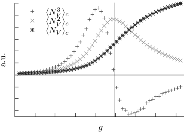
Figure S3: Typical shape of the first three cumulants of the order parameter $N_{V}$, the number of beads of the SHC within the potential range. We locate the adsorption transition by the criterion $\langle N_{V}^{3}\rangle_{c}=0$ in simulations.

An effective method to determine the critical potential strength uses the fact that the derivative of the free energy density with respect to the potential strength $g$ gives the mean fraction of polymer length in the square-well potential, which provides an order parameter for the adsorption transition. For the discrete SHC, we have $\partial_{g}f=\langle N_{V}\rangle/N$, where $N_{V}$ is the number of beads of the SHC within the potential range $0<z<\ell$. Because of the crossover to an effective flexible behavior close to the adsorption transition, we expect a continuous adsorption transition and the second cumulant of the order parameter, i.e., the second derivative $\partial^{2}_{g}f=\langle(N_{V}-\langle N_{V}\rangle)^{2}\rangle=\langle N_{V}^{2}\rangle_{c}$ of the free energy should diverge. Because of finite size effects we find a maximum rather than a divergence in the simulations, which results in a vanishing third cumulant $\partial^{3}_{g}f=\langle N_{V}^{3}\rangle_{c}=0$ at the transition, as shown in Fig. S3. Therefore, we can use the vanishing third cumulant to locate the adsorption transition in simulations. In order to find the zero of the third cumulant we interpolate between the first negative and last positive value to determine the critical potential strength. We use this criterion both for the planar and for curved geometries to locate the adsorption transition.

II.2 Finite size scaling procedure

Finite size scaling of the specific heat allows to determine the critical potential strength $g_{c}$ and to calculate the critical exponent $\nu$ for the correlation length and the free energy. We apply this method to analyze the simulation data for the planar substrate.

To systematically find the best parameter set $(\nu,\,g_{c})$, we calculate a quantity $S(\nu,g_{c})$ which measures the squared differences from one specific heat data set $f$ to the interpolated curves $\tilde{f}$ of another set for different lengthBhattacharjee and Seno (2001) $L$ , as shown in Fig. S4. As contour lengths we use $L/b_{0}=50$, $100$, $150$, $200$, $300$, $400$, $600$ and $800$. To be able to compare different parameter sets $(\nu,\,g_{c})$ we take only the relative differences.

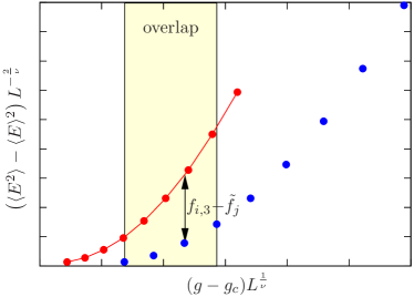
Figure S4: Example for the overlap region of two data sets for $L_{p}=2b_{0}$ and $\ell=b_{0}$ for two different lengths $L=800\,b_{0}$ and $L=400\,b_{0}$. In this example we have $N_{\mathrm{over}}=4$ and use $g_{c}\ell/k_{B}T=0.3$ and $\nu=1.4$.

For this analysis only a limited number $N_{\mathrm{over}}$ of data points in the overlapping region can be used. Our best estimate for $(\nu,\,g_{c})$ is the parameter set that minimizes the overall error

$$S(\nu,g_{c})=\frac{1}{N_{\mathrm{over}}}\sum_{i}\sum_{j\neq i}\sum_{k=1}^{N_{\mathrm{over}}}\left(1-\frac{\tilde{f}_{j}}{f_{i,k}}\right)^{2}$$

The determination of $\nu$ is quite difficult because the minimum is often rather shallow as shown in the example in Fig. S5.

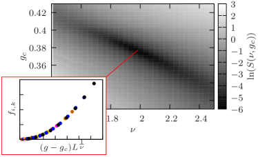
Figure S5: Logarithmic overall error $\ln\left(S(\nu,g_{c})\right)$ as a function of parameters $g_{c}\ell/k_{B}T$ and $\nu$. Inset: Scaling function $f_{i,k}$ for the optimal choices $\nu_{\mathrm{min}}=1.99$ and $g_{c,{\mathrm{min}}}\ell/k_{B}T=0.37$. Analysis for MC data for parameters $L_{p}=2b_{0}$, $k=100k_{B}T/b_{0}^{2}$ and $\ell=b_{0}$.

A simple approach to estimate the error in this procedure is given by Bhattacharjee and Seno (2001)

$$\Delta g_{c} =\eta g_{c,\,\mathrm{min}}\left(2\ln{\frac{S(\nu_{\mathrm{min}},g_{c,\,\mathrm{min}}(1{\pm}\eta))}{S(\nu_{\mathrm{min}},g_{c,\,\mathrm{min}})}}\right)^{{1}/{2}}$$

$$\Delta\nu =\eta\nu_{\,\mathrm{min}}\left(2\ln{\frac{S(\nu_{\mathrm{min}}(1{\pm}\eta),g_{c,\,\mathrm{min}})}{S(\nu_{\mathrm{min}},g_{c,\,\mathrm{min}})}}\right)^{{1}/{2}}\text{ ,}$$

where $\eta\equiv 0.01$ gives the relative distance to the minimum. We note that this method of error estimation might be flawed, because the determination of $g_{c}$ is much more precise than the determination of $\nu$. While changes in $g_{c}$ mainly shift data points in Fig. S4 horizontally and influence the overlap region, variation of $\nu$ affects mostly the rescaled specific heat values $f_{i,k}$ themselves and, thus, shift data points vertically in Fig. S4. If the overlap region becomes smaller the overall error $S(\nu,g_{c})$ increases fast. This explains why the variation of $g_{c}$ influences $S(\nu,g_{c})$ much more than $\nu$ such that the determination of $\nu$ is more difficult. To take this into account, we compute the minimal and maximal value of $g_{c}$ and $\nu$, where $S(\nu,g_{c})<(1+\eta_{2})S(\nu_{\mathrm{min,max}},g_{c,\mathrm{min,max}})$, where $\eta_{2}$ is an arbitrary parameter. These minimal and maximal values for $g_{c}$ and $\nu$ should be a valid estimation of the error.

III Simulation results for critical exponent $\nu$ for planar substrate

The finite size scaling procedure also allows us to determine the critical exponent $\nu$ for adsorption to a planar substrate. Results for the exponent $\nu$ are shown in Fig. S6 as a function of the stiffness parameter $L_{p}/\ell$.

The exponent $\nu$ is around $\nu=2$ for small bending rigidity and lowers towards $\nu=1$ with increasing stiffness. This is in agreement with the theoretical expectation that adsorption of flexible polymers is a continuous transition with $\nu_{F}=2$. A semiflexible polymer should exhibit a critical behavior corresponding to $\nu_{SF}=1$ with a crossover to a flexible behavior with $\nu=\nu_{F}=2$ in the small regime $|g-g_{c,SF}|<k_{B}T/L_{p}$ around the transition, where the correlation length $\xi$ exceeds $L_{p}$ as explained in section I.3.2. This crossover might be the reason that we obtain values $\nu\approx 1.4$ significantly larger than $\nu=1$ for stiff polymers using the finite size scaling.

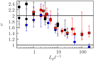
Figure S6: Finite size scaling results for the critical exponent $\nu$ in $D=3$ dimensions (circles) and $D=2$ dimensions (squares) as a function of the dimensionless stiffness parameter $L_{p}/\ell$ for $\ell=1$ (red), $\ell=2$ (blue) and $\ell=4$ (black). Simulation parameters are as in Fig. 4.

IV Additional simulation snapshots

In Fig. S7 we present additional simulation snapshots in the desorbed phase for all three adsorption geometries.

Figure S7: Phase diagrams for a planar substrate (red line), an adsorbing sphere (blue line) and an adsorbing washboard in $D=2$ (brown line) and simulation snapshots in the desorbed phases corresponding to the open circles in the phase diagram. Solid circles correspond to the simulation snapshots in the adsorbed phase presented in the main text.

References

- Skolnick and Fixman (1977) J. Skolnick and M. Fixman, Macromolecules 10, 944 (1977).
- Förster et al. (1999) S. Förster, I. Neubert, A. D. Schlüter, and P. Lindner, Macromolecules 32, 4043 (1999).
- Gutjahr, Lipowsky, and Kierfeld (2006) P. Gutjahr, R. Lipowsky, and J. Kierfeld, Europhys. Lett. 76, 994 (2006).
- Bednar et al. (1995) J. Bednar, P. Furrer, V. Katritch, A. Stasiak, J. Dubochet, and A. Stasiak, J. Mol. Biol. 254, 579 (1995).
- Ott et al. (1993) A. Ott, M. Magnasco, A. Simon, and A. Libchaber, Phys. Rev. E 48, R1642 (1993).
- Venier et al. (1994) P. Venier, A. Maggs, M. Carlier, and D. Pantaloni, J. Biol. Chem. 269, 13353 (1994).
- de Gennes (1979) P. de Gennes, Scaling Concepts in Polymer Physics (Cornell University Press, Ithaca and London, 1979).
- Eisenriegler (1993) E. Eisenriegler, Polymers near Surfaces (World Scientific, London, 1993).
- Netz and Andelman (2003) R. R. Netz and D. Andelman, Phys. Rep. 380, 1 (2003).
- Angelini et al. (2003) T. Angelini, H. Liang, W. Wriggers, and G. Wong, Proc. Nat. Acad. Sci. USA 100, 8634 (2003).
- Dos Remedios et al. (2003) C. Dos Remedios, D. Chhabra, M. Kekic, I. Dedova, M. Tsubakihara, D. Berry, and N. Nosworthy, Physiol. Rev. 83, 433 (2003).
- Winder and Ayscough (2005) S. J. Winder and K. R. Ayscough, J. Cell Sci. 118, 651 (2005).
- Fletcher and Mullins (2010) D. A. Fletcher and R. D. Mullins, Nature 463, 485 (2010).
- Maggs, Huse, and Leibler (1989) A. C. Maggs, D. A. Huse, and S. Leibler, Europhys. Lett. 8, 615 (1989).
- Kierfeld (2006) J. Kierfeld, Phys. Rev. Lett. 97, 058302 (2006).
- Birshtein, Zhulina, and Skvortsov (1979) T. M. Birshtein, E. B. Zhulina, and A. M. Skvortsov, Biopolymers 18, 1171 (1979).
- van der Linden, Leermakers, and Fleer (1996) C. C. van der Linden, F. A. M. Leermakers, and G. J. Fleer, Macromolecules 29, 1172 (1996).
- Kramarenko et al. (1996) E. Kramarenko, R. Winkler, P. Khalatur, A. Khokhlov, and P. Reineker, J. Chem. Phys. 104, 4806 (1996).
- Sintes, Sumithra, and Straube (2001) T. Sintes, K. Sumithra, and E. Straube, Macromolecules 34, 1352 (2001).
- Netz and Joanny (1999a) R. R. Netz and J.-F. Joanny, Macromolecules 32, 9013 (1999a).
- Kong and Muthukumar (1998) C. Y. Kong and M. Muthukumar, J. Chem. Phys. 109, 1522 (1998).
- Caravenna and Deuschel (2008) F. Caravenna and J.-D. Deuschel, Ann. Probab. 36, 2388 (2008).
- Hsu and Binder (2013) H.-P. Hsu and K. Binder, Macromolecules 46, 2496 (2013).
- Freed (1972) K. F. Freed, Adv. in Chem. Phys. 22, 1 (1972).
- Gompper and Burkhardt (1989) G. Gompper and T. Burkhardt, Phys. Rev. A 40, 6124 (1989).
- Gompper and Seifert (1990) G. Gompper and U. Seifert, J. Phys. A: Math. Gen. 23, L1161 (1990).
- Kuznetsov and Sung (1997) D. V. Kuznetsov and W. Sung, J. Chem. Phys. 107, 4729 (1997).
- Bundschuh, Lässig, and Lipowsky (2000) R. Bundschuh, M. Lässig, and R. Lipowsky, Eur. Phys. J. E 3, 295 (2000).
- Stepanow (2001) S. Stepanow, J. Chem. Phys. 115, 1565 (2001).
- Semenov (2002) A. N. Semenov, Eur. Phys. J. E 9, 353 (2002).
- Kierfeld and Lipowsky (2003) J. Kierfeld and R. Lipowsky, Europhys. Lett. 62, 285 (2003).
- Benetatos and Frey (2003) P. Benetatos and E. Frey, Phys. Rev. E 67, 051108 (2003).
- Kierfeld and Lipowsky (2005) J. Kierfeld and R. Lipowsky, J. Phys. A: Math. Gen. 38, L155 (2005).
- Deng et al. (2010) M. Deng, Y. Jiang, H. Liang, and J. Chen, J. Chem. Phys. 133, 034902 (2010).
- Wallin and Linse (1996) T. Wallin and P. Linse, Langmuir 12, 305 (1996).
- Netz and Joanny (1999b) R. R. Netz and J.-F. Joanny, Macromolecules 32, 9026 (1999b).
- Schiessel et al. (2000) H. Schiessel, J. Rudnick, R. Bruinsma, and W. M. Gelbart, Europhys. Lett. 51, 237 (2000).
- Kunze and Netz (2000) K.-K. Kunze and R. R. Netz, Phys. Rev. Lett. 85, 4389 (2000).
- Cherstvy and Winkler (2011) A. G. Cherstvy and R. G. Winkler, Phys. Chem. Chem. Phys. 13, 11686 (2011).
- Cherstvy (2012) A. G. Cherstvy, Biopolymers 97, 311 (2012).
- Hochrein et al. (2007) M. Hochrein, J. Leierseder, L. Golubović, and J. Rädler, Phys. Rev. E 75, 021901 (2007).
- Gutjahr, Lipowsky, and Kierfeld (2010) P. Gutjahr, R. Lipowsky, and J. Kierfeld, Soft Matter , 5461 (2010).
- Kraikivski, Lipowsky, and Kierfeld (2004) P. Kraikivski, R. Lipowsky, and J. Kierfeld, Europhys. Lett. 66, 763 (2004).
- Kraikivski, Lipowsky, and Kierfeld (2005) P. Kraikivski, R. Lipowsky, and J. Kierfeld, Eur. Phys. J. E 16, 319 (2005).
- Pierre-Louis (2011) O. Pierre-Louis, Phys. Rev. E 83, 011801 (2011).
- Kratky and Porod (1949) O. Kratky and G. Porod, Recueil des Travaux Chimiques des Pays-Bas 68, 1106 (1949).
- Harris and Hearst (1966) R. Harris and J. Hearst, J. Chem. Phys. 44, 2595 (1966).
- Kleinert (2006) H. Kleinert, Path Integrals in Quantum Mechanics, Statistics, Polymer Physics, and Financial Markets (World Scientific, Singapore, 2006).
- Odijk (1977) T. Odijk, J. Polym. Sci. 15, 477 (1977).
- Lipowsky (1989) R. Lipowsky, Phys. Rev. Lett. 62, 704 (1989).
- Kierfeld et al. (2004) J. Kierfeld, O. Niamploy, V. Sa-Yakanit, and R. Lipowsky, Eur. Phys. J. E 14, 17 (2004).
- MacKintosh, Käs, and Janmey (1995) F. MacKintosh, J. Käs, and P. Janmey, Phys. Rev. Lett. 75, 4425 (1995).
- Kojima, Ishijima, and Yanagida (1994) H. Kojima, A. Ishijima, and T. Yanagida, Proc. Nat. Acad. Sci. USA 91, 12962 (1994).
- Odijk (1983) T. Odijk, Macromolecules 16, 1340 (1983).
- Köster et al. (2007) S. Köster, H. Stark, T. Pfohl, and J. Kierfeld, Biophys. Rev. Lett. 2, 155 (2007).
- Köster, Kierfeld, and Pfohl (2008) S. Köster, J. Kierfeld, and T. Pfohl, Eur. Phys J. E 25, 439 (2008).
- (57) See supplementary material (appended) for additional information.
- Binder (1987) K. Binder, Rep. Prog. Phys. 50, 783 (1987).
- Pierre-Louis (2008) O. Pierre-Louis, Phys. Rev. E 78, 021603 (2008).
- Li and Zhang (2010) T. Li and Z. Zhang, J. Phys. D: Appl. Phys. 43, 075303 (2010).
- Zhang, Ohbu, and Dubin (2000) H. Zhang, K. Ohbu, and P. L. Dubin, Langmuir 16, 9082 (2000).
- Cooper et al. (2006) C. L. Cooper, A. Goulding, a. B. Kayitmazer, S. Ulrich, S. Stoll, S. Turksen, S.-i. Yusa, A. Kumar, and P. L. Dubin, Biomacromolecules 7, 1025 (2006).