Photospheric Emission From Stratified Jets

Abstract

We explore photospheric emissions from stratified two-component jets, wherein a highly relativistic spine outflow is surrounded by a wider and less relativistic sheath outflow. Thermal photons are injected in regions of high optical depth and propagated until they escape at the photosphere. Due to the presence of shear in velocity (Lorentz factor) at the boundary of the spine and sheath region, a fraction of the injected photons are accelerated via a Fermi-like acceleration mechanism such that a high energy power-law tail is formed in the resultant spectrum. We show, in particular, that if a velocity shear with a considerable variance in the bulk Lorentz factor is present, the high energy part of observed Gamma-ray Bursts (GRBs) photon spectrum can be explained by this photon acceleration mechanism. We also show that the accelerated photons may also account for the origin of the extra hard power-law component above the bump of the thermal-like peak seen in some peculiar bursts (e.g., GRB 090510, 090902B, 090926A). It is demonstrated that time-integrated spectra can also reproduce the low energy spectrum of GRBs consistently due to a multi-temperature effect when time evolution of the outflow is considered. Finally, we show that the empirical $E_{\rm p}$-$L_{\rm p}$ relation can be explained by differences in the outflow properties of individual sources.

1. INTRODUCTION

Gamma-ray Bursts (GRBs) are the most powerful explosions in the Universe. Prompt emission of GRBs are mainly observed in the energy range of 10 keV - MeV and show rapid time variability in their lightcurves. Their spectra are often modeled by an empirical ’Band’ function (Band et al., 1993; Preece et al., 2000; Kaneko et al., 2006, 2008), which is a smoothly jointed broken power-law, whose physical origin is not yet identified. The typical low and high energy photon indices are distributed around $\alpha_{\rm ph}\sim-1$ and $\beta_{\rm ph}\sim-2.5$, respectively, while the spectral peak (break) energy is distributed around $E_{\rm p}\sim$ a few $100~{}{\rm keV}$.

The most widely discussed model for the prompt emission mechanism is the internal shock model (Rees & Meszaros, 1994; Sari & Piran, 1997). In this model, it is assumed that relativistically moving shells emanate from the central engine with diverse velocities, and shocks form due to collisions of the shells. Shocks are accompanied by particle acceleration, and eventually gamma-rays are produced by relativistic electrons via synchrotron radiation. The internal shock model can naturally explain the observed rapid time variability in the lightcurve and non-thermal nature of the spectra. However, it is known that the model suffers from poor radiation efficiency, since only the kinetic energy associated with the relative motion of shells can be released (Kobayashi et al., 1997; Lazzati et al., 1999; Guetta et al., 2001; Kino et al., 2004). This contradicts with observations which show high efficiencies of a few tens of percent (Fan & Piran, 2006; Zhang et al., 2007). Another difficulty is the low energy spectral index ($\alpha_{\rm ph}$). A non-negligible fraction of observed GRBs show hard spectra at low energies which cannot be explained by synchrotron emission (Crider et al., 1997; Preece et al., 1998; Ghirlanda et al., 2003).

These well-known difficulties in the internal shock model have lead researchers to reconsider photospheric emission (e.g., Thompson, 1994; Eichler & Levinson, 2000; Mészáros & Rees, 2000; Rees & Mészáros, 2005; Lazzati et al., 2009; Beloborodov, 2011; Pe’er & Ryde, 2011; Mizuta et al., 2011; Nagakura et al., 2011; Ruffini et al., 2011; Xu et al., 2012; Bégué et al., 2013; Lundman et al., 2013; Lazzati et al., 2013), which is a natural consequence of the original fireball model (Goodman, 1986; Paczynski, 1986). In this model, prompt gamma-rays are released at the photosphere when the fireball becomes optically thin. The peak energy of the spectra is determined by the temperature at the photosphere. This model has an advantage in that high emission efficiencies can be naturally achieved. Strong observational support for this scenario has been provided by the recent detection of quasi-thermal emission by the Fermi Large Area Telescope (LAT), notably GRB 090902B (Abdo et al., 2009; Ryde et al., 2010, 2011; Pe’er et al., 2012).

However, while there are many advantages, the photospheric emission model must overcome several difficulties. The major flaw is reproduction of the observed broad non-thermal spectra, since the photons that originate from regions of very high optical depths are inevitably thermalized. Photospheric emission can, in principle, explain the hard low-energy spectra that cannot be accounted for by synchrotron emission, by considering a superposition of emission components which have different temperatures (multi-color Blackbody). This is because the Rayleigh-Jeans part of the emission component has a much harder photon index ($\alpha_{\rm ph}=1$) than those inferred in all observed GRBs. It is noted, however, that the existence of outflow models that can naturally account for the low energy spectra is still debated. Recent theoretical studies which explore peak energies of photospheric emissions based on spherical (one-dimensional) outflow models (e.g., Levinson, 2012; Beloborodov, 2013; Vurm et al., 2013) suggest that it is difficult to regulate the temperature of the emissions to be well below the typical observed peak energies $E_{\rm p}$, particularly when dissipation is present (but see, e.g., Levinson & Globus, 2013, for a mechanism that may overcome this difficulty). Although dissipative processes are not considered, an outflow structure in two-dimensions suggested by (Lundman et al., 2013) may be a key ingredient to resolve this difficulty. Based on hydrodynamical simulations of jet propagation (Zhang et al., 2003), Lundman et al. (2013) modeled an outflow with a Lorentz factor gradient in the lateral direction. By solving the transfer of photons within the jet, they indeed showed that the low energy spectra can be reproduced by the multi-color temperature effects due to the superposition of the photons released from different lateral positions that have various Lorentz factors.

On the other hand, the high energy part of the observed spectra is difficult to reproduce by the super-position of thermal emissions, since an unreasonably high temperature must be realized within the outflow. To overcome this difficulty, dissipative processes around the photosphere have been suggested in previous studies. Various mechanisms such as shocks (Pe’er et al., 2005, 2006; Ioka et al., 2007; Lazzati & Begelman, 2010), magnetic reconnection (Giannios, 2006; Giannios & Spruit, 2007; Giannios, 2008) and proton-neutron nuclear collisions (Beloborodov, 2010; Vurm et al., 2011) have been proposed. All models are accompanied by the generation of relativistic electrons (and positrons) that upscatter the thermal photons to create the non-thermal spectra (Giannios, 2012). However, it is quite uncertain whether dissipative processes can operate efficiently enough to deposit in relativistic electrons (and positrons) the copious amounts of energy needed to reproduce observations.

Although the details are not well studied, Fermi-like acceleration of photons at the shocks formed below the photosphere due to bulk Compton scattering can be regarded as an alternative mechanism for producing high energy non-thermal spectra (Eichler, 1994). Presence of relativistic electrons (and positrons) is not required in this scenario, since the energy of the background fluid can be directly transferred to the photons as they propagate. Shocks formed below the photosphere are inevitably mediated by radiation (Levinson & Bromberg, 2008). The properties of relativistic radiation mediated shocks have been explored in various astrophysical contexts (e.g., shock breakouts) including GRBs. The most detailed and fully self-consistent analysis of relativistic radiation mediated shocks have been performed by Budnik et al. (2010) (see also Katz et al., 2010). Although not as sophisticated as the above study, Bromberg et al. (2011) explored the properties of photon acceleration in the context of shocks within GRB jets. These studies have shown that the existence of accelerated photons above the thermal peak energy is an inherent feature in these shocks. However, all the above studies assume a one-dimensional stationary planar shock in their analysis, and the obtained spectra are far from those typically observed. Therefore, for a more accurate estimation, a global photon transfer calculation incorporating the multi-dimensional structure of the jet must be performed. Ioka et al. (2011) explored the properties of shocks that are formed in radiation dominated jets. They claimed that photons which are accelerated at the shock can generate a spectra which are close to the ’Band’ function. However, since their argument is based on a simple analytical framework in which the transfer of photons is not solved, it is obvious that detailed calculations are required to form firmer conclusions.

While the previous studies focused on the shocks, any form of large velocity gradients that are present in the outflow can give rise to photon acceleration. For instance, a Fermi-like mechanism can also operate when velocity shear exists in the transverse direction of the outflow, just as in the case of the acceleration of the cosmic rays (e.g., Jokipii et al., 1989; Ostrowski, 1990, 1998). Indeed, GRB jets are likely to posses rich internal velocity structures in the transverse directions. For example, numerical studies which explore the launching mechanism of the relativistic jets suggest that the produced jets have transversely stratified structures in which the bulk Lorentz factor increases towards the jet axis (McKinney, 2006; Nagataki et al., 2007; Nagataki, 2009; McKinney & Blandford, 2009; Nagataki, 2011). Since the highly magnetized jets seen in these simulations are cold, subsequent magnetic field dissipation must occur in order to produce a hot fireball which leads to an efficient photospheric emission. Although the flow structure after the dissipative process is highly uncertain, the stratified structure that originated at the central engine may remain even at this stage. Moreover, rich velocity structure can also develop after the launching phase as the jets drill through the progenitor star envelopes. A large number of hydrodynamic simulations regarding the jet propagation show that large velocity gradients appear within the jet (in radial as well as transverse directions) due to the interaction with the stellar envelope (Zhang et al., 2003; Mizuta et al., 2006; Morsony et al., 2007; Lazzati et al., 2009; Mizuta et al., 2011; Nagakura et al., 2011). Notably, large velocity gradient in the transverse directions produced by the strong recollimation shocks seen in these studies will likely provide an efficient acceleration site for photons as pointed out by Levinson (2012).

Motivated by this background, we explore the photon acceleration within a jet with velocity structures in the transverse direction and its effect on the resulting spectra of the photospheric emissions by solving the transfer of photons. As mentioned earlier, mainly focusing on the origin of the low energy spectra, Lundman et al. (2013) carried out a similar study. By performing a photon transfer calculation, they evaluated the photospheric emission from a relativistic jet that has a continuously decaying velocity profile in lateral direction $\Gamma\propto\theta^{-p}$ at the outer region. However, while they succeeded in reproducing the spectra below the peak energy, the imposed velocity gradient was not large enough to trigger efficient photon acceleration and, therefore, the high energy part was too soft compared to the Band spectra. With the aim to investigate the cases with efficient photon accelerations, we focus on jets that have a velocity shear in the transverse direction. This can be considered as a limiting case of $p=\infty$ in Lundman et al. (2013) work, a parameter region which was not explored. As a first step, this study considers a simple stratified two-component jet structure, wherein a highly relativistic spine outflow is surrounded by a wider and less relativistic sheath outflow. We show, in particular, that the high-energy part of the Band spectra (photon index $\beta_{\rm ph}$) can indeed be reproduced by photons accelerated at the shear layer. In addition, we also demonstrate that the low-energy part of the spectra (photon index $\alpha_{\rm ph}$) can be reproduced consistently within the framework of the present study when time evolution of the outflow is considered.

The paper is organized as follows. In §2, we describe our model and numerical procedures. We present our main results in §3. Discussions of the implications of our results are given in §4. The summary of our main findings are given in §5.

2. MODEL AND METHODS

In the present study, we evaluate the photospheric emissions from an ultra-relativistic outflow which has a spine-sheath jet structure. The spine is defined as a region of conical outflow with a half-opening angle $\theta_{0}$, while the sheath is a region of outflow which surrounds the spine and extends up to an angle of $\theta_{1}(>\theta_{0})$ (see Fig. 1). Each region has different fluid properties and a steady radial outflow is assumed.

2.1. Fluid Properties of Spine-Sheath Jet

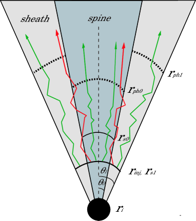
Figure 1.— Schematic picture of the employed model. A fast spine jet is embedded in a slower sheath outflow. Spine and sheath start to accelerate at a radius $r_{\rm i}$, and the acceleration continues up to $r_{\rm s0}$ and $r_{\rm s1}$ in the spine and sheath region, respectively. Since the dimensionless entropy of the spine $\eta_{0}$ is larger than that of the sheath $\eta_{1}$, the saturation radius and the terminal Lorentz factor of the spine ($r_{\rm s0}=\eta_{0}r_{\rm i}$ and $\Gamma_{0}=\eta_{0}$) are larger than that of the sheath ($r_{\rm s1}=\eta_{1}r_{\rm i}$ and $\Gamma_{1}=\eta_{1}$). The photospheric radius of the spine $r_{\rm ph0}$ is smaller than that of the sheath $r_{\rm s1}$. In our model, thermal photons are injected at a the saturation radius of the sheath $r_{\rm inj}=r_{\rm s1}$, and the transfer is solved up to the radius in which the optical depth is much lower than unity. Photons which cross the boundary layer of the spine and sheath multiple times gain energy and produce a non-thermal tail in the resultant spectrum.

2.1.1 Radial evolution

Under the assumption that the energy density in the magnetic field and the dissipated kinetic energy are sub-dominant, the fluid properties of the spine and sheath regions are described by the standard adiabatic “fireball” model (e.g., Piran, 2004; Mészáros, 2006). Here we give a brief review of the fireball model and show how the radial evolution of the Lorentz factor (velocity), $\Gamma$, and electron number density, $n_{e}$, which are necessary background fluid information for evaluating the photon transfer, is determined.

The dynamics of the fireball can be characterized by three independent parameters, which are the initial fireball radius, $r_{\rm i}$, the kinetic luminosity, $L$, and the dimensionless entropy which characterizes the baryon loading, $\eta\equiv L/\dot{M}c^{2}$, where $\dot{M}$ and $c$ are the mass outflow rate and the speed of light, respectively. Initially, the fireball accelerates as it expands by converting its internal energy into kinetic energy (acceleration phase). As a result, the bulk Lorentz factor of the flow increases with radius, $r$, as $\Gamma(r)\simeq(r/r_{\rm i})$. If $\eta$ is larger than the critical value given by $\eta_{c}=(\sigma_{\rm T}L/8\pi r_{\rm i}m_{p}c^{3})^{1/4}$ (Piran, 2004; Mészáros, 2006), the fireball becomes transparent to radiation during the acceleration phase, where $\sigma_{T}$ and $m_{p}$ are the Thomson cross section and proton rest mass, respectively. On the other hand, if $\eta<\eta_{c}$, the fireball becomes transparent after the acceleration has ceased and the flow asymptotically approaches a constant Lorentz factor $\Gamma=\eta$ (coasting phase). In this case, the acceleration continues up to the saturation radius, $r_{\rm s}=\eta r_{\rm i}$. In the present study, we focus on the latter case and consider the parameter space in which $\eta<\eta_{c}$ is satisfied in both the spine and sheath regions. Hence, the radial evolution of Lorentz factor is given by

$$\Gamma(r)=\left\{\begin{array}[]{ll}\frac{r}{r_{\rm s}}&~{}~{}{\rm for}~{}~{}r\leq r_{\rm s},\\ \eta&~{}~{}{\rm for}~{}~{}r>r_{\rm s}.\\ \end{array}\right.$$ (3)

In the relativistically expanding outflow, the electron number density in the comoving frame is given by

$$n_{e}(r)=\frac{\dot{M}}{4\pi r^{2}m_{p}\Gamma\beta c}=\frac{L}{4\pi r^{2}m_{p}\eta\Gamma\beta c^{3}},$$ (4)

where $\beta$ is the velocity of the flow normalized by the speed of light. Here, we assumed that there are no strong dissipative processes in the outflow which may create copious pair plasma. Since we consider the case of $\eta<\eta_{c}$, the electron number density decreases with radius as $n_{e}\propto r^{-3}$ below the saturation radius ($r\leq r_{\rm s}$) and as $n_{e}\propto r^{-2}$ at larger radii ($r>r_{\rm s}$).

Given the electron number density and bulk Lorentz factor of the flow, the optical depth to Thomson scatterings for the photons propagating in the radial direction to reach infinity can be evaluated as

$$\tau(r) = \int^{\infty}_{r}\sigma_{\rm T}n_{e}(r^{\prime})\Gamma(r^{\prime})(1-\beta(r^{\prime}))dr^{\prime}$$ (7)

$$\simeq \left\{\begin{array}[]{ll}\frac{r_{\rm ph}}{r}\left[1+\frac{1}{3}\left\{\left(\frac{r_{\rm s}}{r}\right)^{2}-\left(\frac{r}{r_{\rm s}}\right)^{2}\right\}\right]&~{}~{}{\rm for}~{}~{}r\leq r_{\rm s},\\ \frac{r_{\rm ph}}{r}&~{}~{}{\rm for}~{}~{}r>r_{\rm s},\par\\ \end{array}\right.$$

$$r_{\rm ph}=\frac{\sigma_{\rm T}L}{8\pi\eta^{3}m_{p}c^{3}},$$ (8)

where we have assumed $\Gamma\gg 1$. Here, $r_{\rm ph}$ is the photospheric radius which corresponds to the radius where the optical depth becomes unity ($\tau=1$).

2.1.2 Spine-sheath structure

The radial profiles of the fluid quantities ($n_{e}(r)$ and $\Gamma(r)$) in the spine and sheath regions are different, since we impose different values on their fireball parameters ($r_{\rm i}$, $L$ and $\eta$). In the present study, while we assume the same value for $r_{\rm i}$ in both regions, the dimensionless entropy of the spine, $\eta_{0}$, is taken to be larger than that of the sheath, $\eta_{1}$. Hence, the saturation radius in the spine region, $r_{\rm s0}=\eta_{0}r_{\rm i}$, is larger than that of the sheath, $r_{\rm s1}=\eta_{1}r_{\rm i}$, and the terminal Lorentz factor of the former ($\eta_{0}$) is larger than that of the latter ($\eta_{1}$). Regarding the evolution of the Lorentz factor in the spine and sheath, they have equal values ($\Gamma_{0}(r)=\Gamma_{1}(r)=r/r_{\rm i}$) up to $r=r_{\rm s1}$. At larger radii ($r>r_{\rm s1}$), velocity shear begins to develop and the difference in the Lorentz factor increases with radius up to $r_{\rm s0}$, since the spine is in the acceleration phase while the sheath is in the coasting phase ($\Gamma_{1}=\eta_{1}$). Thereafter, the spine also enters the coasting phase ($\Gamma_{0}=\eta_{0}$), and the difference in the Lorentz factor is constant. In determining the kinetic luminosities of the spine, $L_{0}$, and sheath, $L_{1}$, we assume that the mass outflow rate is equal in both regions ($L_{0}/\eta_{0}=L_{1}/\eta_{1}$). Therefore, kinetic luminosity of the spine is larger by a factor of $\eta_{0}/\eta_{1}$. Under these assumptions, the photospheric radius in the sheath, $r_{\rm ph1}$, is larger than that in the spine, $r_{\rm ph0}$, by a factor of $(\eta_{0}/\eta_{1})^{2}$ (see equation (8)). A schematic picture of the employed model is given in Fig. 1.

Hereafter, the quantities corresponding to the spine and sheath regions are denoted by subscript $0$ and $1$, respectively.

2.2. Photon Transfer in a Spine-Sheath Jet

Having determined the background fluid properties ($\Gamma$ and $n_{e}$), we evaluate the resultant photospheric emission by solving the propagation of photons which are injected far below the photosphere. The photon transfer is evaluated by performing a three-dimensional test particle Monte-Carlo simulation. In GRB jets, opacity of photons is strongly dominated by the scatterings with electrons. Therefore, we neglect the absorption process and only consider the scattering process by the electrons in our calculations. Furthermore we do not take into account the thermal motion of the electrons in evaluating the scattering for simplicity.

2.2.1 Initial condition

Initially, the photons are injected within the jet at the surface of a fixed radius where the velocity shear begins to develop $r_{\rm inj}=r_{\rm s1}$. For the cases considered in this study, $r_{\rm inj}$ is always located far below the photosphere ($\tau(r_{\rm inj})\gg 1$). Therefore, a tight coupling between the photons and matter is expected. For this reason, we can safely assume that the photons have an isotropic distribution with energy distribution given by a Planck distribution in the comoving frame. According to the fireball model, the radial evolution of the comoving temperature is given by

$$T^{\prime}(r)=\left\{\begin{array}[]{ll}\left(\frac{L}{4\pi r_{\rm i}^{2}ca}\right)^{1/4}\left(\frac{r}{r_{\rm i}}\right)^{-1}&~{}~{}{\rm for}~{}~{}r\leq r_{\rm s},\\ \left(\frac{L}{4\pi r_{\rm i}^{2}ca}\right)^{1/4}\left(\frac{r_{\rm s}}{r_{\rm i}}\right)^{-1}\left(\frac{r}{r_{\rm s}}\right)^{-2/3}&~{}~{}{\rm for}~{}~{}r>r_{\rm s},\\ \end{array}\right.$$ (11)

where $a$ is the radiation constant. Hence, we adopt the temperature at the corresponding radius given by above equation $T^{\prime}_{\rm inj}=T^{\prime}(r_{\rm inj})$ for the comoving temperature of the injected photons. While the photons are isotropic in the comoving frame, they are strongly beamed in the laboratory frame due to the Doppler boosting effect. Due to this effect, the radiation intensity of the blackbody emission in the laboratory frame is given by

$$I_{\nu,{\rm inj}}(\nu)={\cal D}(\Gamma_{\rm inj},\theta_{v})^{3}B_{\nu}(T^{\prime}_{\rm inj},\nu/{\cal D}(\Gamma_{\rm inj},\theta_{v})),$$ (12)

where $\Gamma_{\rm inj}=\Gamma(r_{\rm inj})$ is the bulk Lorentz factor of the flow at $r=r_{\rm inj}$ determined from equation (3). Here, $B_{\nu}(T^{\prime},\nu)=2h\nu^{3}c^{-2}[{\rm exp}(h\nu)/k_{\rm B}T^{\prime}-1]^{-1}$ is the Planck function, where $h$ and $k_{\rm B}$ are the Planck constant and the Boltzmann constant, respectively, and $D(\Gamma,\theta_{v})=[\Gamma(1-\beta{\rm cos}\theta_{v})]^{-1}$ is the Doppler factor, where $\theta_{v}$ is the angle between the photon propagation direction and the fluid velocity direction (radial direction). In our calculations, the initial propagation direction and frequency of the injected photons are drawn from a source of photons given by the above equation.

It is emphasized that the results of our calculation are insensitive to the assumed position of the injection radius as long as $r_{\rm inj}\leq r_{\rm s1}$ is satisfied. This is because, at a radius far below the photosphere ($\tau(r)\gg 1$), the photon energy distribution evaluated by solving the photon transfer does not deviate from the Planck distribution if velocity shear is not present (see next section), and its temperature evolution is well described by equation (11). The temperature of the injected photons in the spine, $T^{\prime}_{\rm inj0}$, is higher than that in the sheath, $T^{\prime}_{\rm inj1}$, by a factor of $(\eta_{0}/\eta_{1})^{1/2}$, since the kinetic luminosity of the former is higher by a factor of $(\eta_{0}/\eta_{1})^{2}$. Correspondingly, the luminosity of the injected photons in the laboratory frame ($L_{\rm inj}\propto r_{\rm inj}^{2}\Gamma_{\rm inj}^{2}T_{\rm inj}^{{}^{\prime}4}$) in the spine is higher than that of the sheath by a factor $\sim(T^{\prime}_{\rm inj0}/{T^{\prime}}^{4}_{\rm inj1})\sim(\eta_{0}/\eta_{1})^{2}$.

2.2.2 Boundary conditions

After the photons are injected, we track their path within the jet in three-dimensions by performing Monte-Carlo simulations (§2.2.3) until they reach the outer or inner boundary of the calculation. Using spherical coordinates ($r$,$\theta$,$\phi$), the outer boundary $r$ is set at a radius $r_{\rm out}=500r_{\rm ph0}$ where the photons can be safely considered to have escaped since the optical depth is $\tau(r_{\rm out})=2\times 10^{-3}\ll 1$. While there is no boundary in the $\phi$ direction, outer boundary in the $\theta$ direction is set at $\theta_{\rm out}=\theta_{1}$ which corresponds to the edge of the whole jet. As for the inner boundary, we adopt a radius slightly below the injection radius $r_{\rm in}=0.5r_{\rm inj}$. For photons which have reached the outer boundaries, we assume that they escape freely to $r=\infty$ without being scattered or absorbed. On the other hand, we assume that the photons are simply absorbed in the inner boundary. It is noted, however, that the fraction of absorbed photons is negligible, since most of the photons in ultra-relativistic outflows are strongly collimated due to the relativistic beaming effect and essentially streamed outward (e.g., Pe’er & Ryde, 2011; Beloborodov, 2011).

The spectra of the emission are evaluated from the photons which have reached the outer boundaries. Due to the relativistic beaming effect, these photons are highly anisotropic and mostly concentrated within a cone of half-opening angle $\sim\Gamma^{-1}$ in the direction of the fluid velocity (radial direction) at the last scattering position. Hence, the observed emission spectra depend significantly on the angle between the direction to the observer and the jet axis, $\theta_{\rm obs}$. In the present study, we evaluate the spectrum for observers located at direction $\theta_{\rm obs}$ by recording all photons which have reached the outer boundary that are propagating in direction within a cone of half-opening angle $\Gamma^{-1}$, which is small enough to regard that the emission is uniform within the cone. From the recorded photon flux, we calculate the isotropic equivalent luminosity by multiplying the photon flux by a factor $4\pi/d\Omega$, where $d\Omega=2\pi[1-{\rm cos}(1/\Gamma)]$ is the solid angle of the cone.

2.2.3 Monte-Carlo simulation for solving photon transfer

Here we briefly describe the Monte-Carlo code used to solve the photon transfer. As noted previously, we neglect the thermal motions of the electrons and only take into account the scattering processes. Hence, the rest frame of the fluid is equivalent to that of the electrons. Under the above assumptions, the propagation of the photons is performed by directly tracking the path of the individual photons in the three-dimensional space of the calculation. Each photon has a specified position propagation direction and frequency, and these quantities are updated by using a uniform random number.

Within the jet, the photons travel along straight paths before they are scattered by the electrons. Firstly, the code determines the distance for the photons to travel before the scattering by drawing the corresponding optical depth $\delta\tau$. The probability for the selected optical depth to be in the range of [$\delta\tau$, $\delta\tau+d\tau$] is given as ${\rm exp}(-\delta\tau)d\tau$. Then, from the given optical depth $\delta\tau$, the distance $l$ to the scattering event is determined from the integration along the straight path of photons which can be expressed as

$$\delta\tau=\int^{l}_{0}n_{e}\Gamma(1-\beta{\rm cos}\theta_{v})\sigma_{\rm sc}dl,$$ (13)

where $\theta_{v}$ is the angle between the direction of fluid velocity and photon. Here, $\sigma_{\rm sc}$ is the total cross section for the electron scattering and is given as

$$\sigma_{\rm sc}=\left\{\begin{array}[]{ll}\sigma_{\rm T}&~{}~{}{\rm for}~{}~{}h\nu_{\rm cmf}\leq 100~{}{\rm keV},\\ \sigma_{\rm KN}&~{}~{}{\rm for}~{}~{}h\nu_{\rm cmf}>100~{}{\rm keV},\\ \end{array}\right.$$ (16)

in our code, where $\sigma_{\rm KN}$ is the total cross section for Compton scattering, and $\nu_{\rm cmf}$ is the frequency of the photon in electron (fluid) comoving frame. (The frequency $\nu_{\rm cmf}$ is evaluated by performing a Lorentz transformation using local fluid velocity). Given the distance $l$ from the above equation, we update the position of the photons to the scattering position by shifting them from the initial position with the given distance in the initial direction of photon propagation. Note that, unlike the case of equation (7), the optical depth calculated by equation (13) is not limited to photons propagating in the radial direction. The path of integration is along the straight path of photons which can be in an arbitrary direction. For a given value of $\delta\tau$, the distance $l$ strongly depends on the propagation direction of the photons in the case of a relativistic flow ($\Gamma\gg 1$). As is obvious from the above equation, the mean free path of photons $l_{\rm mfp}=[n_{e}\Gamma(1-\beta{\rm cos}\theta_{v})]^{-1}$ is quite sensitive to the photon propagation direction, since the factor $\Gamma(1-\beta{\rm cos}\theta_{v})$ varies largely from $\sim(2\Gamma)^{-1}$ (for ${\rm cos}\theta_{v}=-1$) up to $\sim 2\Gamma$ (for ${\rm cos}\theta_{v}=1$) depending on the value of $\theta_{v}$. Hence, a photon tends to travel a larger distance in the fluid velocity (radial) direction since the mean free path of the photon tends to be larger. Hereafter, quantities measured in the comoving frame of the fluid (electron) are denoted by tilde.

In evaluating the integration in equations (13), we employ two different methods depending on the frequency and position of the photon. For photons located above the saturation radius $r\geq r_{\rm s}$ ($\Gamma={\rm const}$) that satisfy $h\nu_{\rm cmf}\leq 100~{}{\rm keV}$ ($\sigma_{\rm sc}=\sigma_{\rm T}={\rm const}$), analytical integration can be performed as shown by Pe’er (2008). Consider a photon path originating from a radius $r_{\rm I}$ that has an angle $\theta_{v,{\rm I}}$ with respect to the fluid velocity (radial) direction at the original position. In this case, the optical depth to reach a radius $r_{\rm II}$ along the straight photon path can be expressed as

$$\Delta\tau_{\rm I-II} = 2\Gamma^{2}r_{\rm ph}\left[\frac{\theta_{v,{\rm II}}}{r_{\rm II}{\rm sin}\theta_{v,{\rm II}}}-\frac{\theta_{v,{\rm I}}}{r_{\rm I}{\rm sin}\theta_{v,{\rm I}}}+\beta\left(\frac{1}{r_{\rm I}}-\frac{1}{r_{\rm II}}\right)\right]$$ (17)

$$= 2\Gamma^{2}\frac{r_{\rm ph}}{r_{\rm I}}\left[\frac{\theta_{v,{\rm II}}-\theta_{v,{\rm I}}}{{\rm sin}\theta_{v,{\rm I}}}+\beta\left(1-\frac{{\rm cos}\theta_{v,{\rm II}}}{{\rm cos}\theta_{v,{\rm I}}}\right)\right],$$

where $\theta_{v,{\rm II}}$ is the photon angle at the final position ($r=r_{\rm II}$). In the second equality, we have used the relation $r_{\rm I}{\rm sin}\theta_{v,{\rm I}}=r_{\rm II}{\rm sin}\theta_{v,{\rm II}}$ that holds for an arbitrary straight line. Hence, in this case, we determine the corresponding propagation length $\Delta l_{\rm I-II}=r_{\rm II}{\rm cos}\theta_{v,{\rm II}}-r_{\rm I}{\rm cos}\theta_{v,{\rm I}}$ from the drawn optical depth by solving equations (17). (Note that equation (17) is solved separately in the spine and sheath region, since the values of $r_{\rm ph}$ and $\Gamma$ $(\beta)$ are different in each region).

On the other hand, when the photons have higher energies ($h\nu_{\rm cmf}>100~{}{\rm keV}$) or are located below the saturation radius ($r<r_{\rm s}$), the integration is solved numerically. In this case, we divide the calculation region into a mesh in spherical coordinates ($r$,$\theta$,$\phi$). Then the integration is done by assuming that the physical quantities (velocity and number density) within the individual mesh are uniform and have the values corresponding to those at the position of the mesh center. We adopt 500 grid points which are logarithmically spaced for the mesh in the $r$ coordinate between the inner boundary $r_{\rm in}$ and outer boundary $r_{\rm out}$. As for the mesh in the $\theta$ coordinate, we adopt 800 uniformly spaced grid points in the range $\theta\leq\theta_{1}$. 1600 uniformly spaced grid points are adopted for the $\phi$ coordinate ($0\leq\phi<2\pi$). It is noted that the resolution of the grid is sufficiently high to reproduce the result obtained by the analytical solution given by equation (17) (corresponding to infinite resolution) in cases when $r\geq r_{\rm s}$ and $h\nu_{\rm cmf}\leq 100~{}{\rm keV}$ are satisfied.

Given the position for the scattering from the above procedure, the four-momentum (the energy and propagation direction) of a photon after the scattering is determined based on the differential cross section for Thomson and Compton scattering. In our code, the scattering process is evaluated in the rest frame of the fluid (electron). First, the four-momentum of the photon before the scattering is Lorentz transformed into the fluid rest frame. For the photons that satisfy $h\nu_{\rm cmf}\leq 100~{}{\rm keV}$, the differential Thompson cross section is used, while the differential Compton cross section is used at higher energies ($h\nu_{\rm cmf}>100~{}{\rm keV}$). The scattering angle or equivalently the propagation direction of the outgoing photon in the fluid rest frame is drawn from the differential cross sections. Regarding the energy of the outgoing photons, we assume that it is conserved before and after the scattering (elastic scattering) in the case of Thomson scattering ($h\nu_{\rm cmf}\leq 100~{}{\rm keV}$). On the other hand, in the case of Compton scattering ($h\nu_{\rm cmf}>100~{}{\rm keV}$), energy loss due to the recoil effect is properly taken into account. The code then Lorentz transforms the outgoing photon four-momentum back into the laboratory frame.

The above procedure is repeated until all the injected photons reach the boundary of the simulation grids.

3. RESULTS

In this section, we show the obtained photon spectra based on the model described in the previous section. We inject $N=2\times 10^{8}$ photon packets in each calculation. In all cases, we employ a fixed value of $\theta_{1}=1^{\circ}$ for the half opening-angle of the jet, which is smaller than that of the typically observed values. It is emphasized, however, that the resulting spectra do not vary for wider jets (larger $\theta_{1}$) as long as the observer angle stays in the range $\theta_{\rm obs}\lesssim\theta_{1}-\Gamma^{-1}$. This is simply because the emission from regions located at a angle $|\theta-\theta_{\rm obs}|\gtrsim\Gamma^{-1}$ is negligible due to the relativistic beaming effect. Therefore, merely to reduce computational cost, we adopt the relatively small value in this study. We use $r_{\rm i}=10^{8}~{}{\rm cm}$ for the initial radius of the fireball in all cases.

3.1. Uniform (Non-Stratified) Jet

Before we look at a stratified jet, we first present results for a one-component uniform jet that does not have structures in the $\theta$ direction ($\theta_{0}=\theta_{1}=1^{\circ}$). In this case, a thermal spectrum is expected, in contrast to a stratified jet as we will discuss later. The isotropic equivalent kinetic luminosity and the dimensionless entropy (terminal Lorentz factor) are set to be $L_{0}=10^{53}{\rm erg/s}$ and $\eta_{0}=400$, respectively. As described in the previous section, we inject the photons at a radius of $r_{\rm inj}=4\times 10^{10}\eta_{0,400}r_{\rm i,8}~{}{\rm cm}$ with intensity given by a blackbody of temperature $k_{\rm B}T^{\prime}_{\rm inj}=1.7r_{\rm i,8}^{-1/2}\eta_{0,400}^{-1}L_{0,53}^{1/4}~{}{\rm keV}$ (see §2 for detail), where $\eta_{0,400}=\eta_{0}/400$, $L_{0,53}=L_{0}/10^{53}~{}{\rm erg/s}$ and $r_{\rm i,8}=r_{\rm i}/10^{8}~{}{\rm cm}$. The corresponding optical depth at the injection radius is $\tau(r_{\rm inj})\sim 23$. The results are insensitive to the value of $r_{\rm inj}$ as long as $\tau\gg 1$ is satisfied as noted in §2. The advected photons lose energy adiabatically due to the expansion of the flow until the coupling with matter becomes weak near the photosphere ($r_{\rm ph0}\simeq 9.2\times 10^{11}L_{0,53}\eta_{0,400}^{-3}~{}{\rm cm}$). The expected temperature at the photosphere can be calculated as $k_{\rm B}T^{\prime}_{\rm ph0}=0.38r_{\rm i,8}^{1/6}\eta_{0,400}^{5/3}L_{0,53}^{-5/12}~{}{\rm keV}$. The observed peak energy of the photospheric emission is expected to be $E_{\rm p}\sim 8\eta_{0}k_{\rm B}T^{\prime}_{\rm ph0}\sim 660r_{\rm i,8}^{1/6}\eta_{0,400}^{8/3}L_{0,53}^{-5/12}~{}{\rm keV}$, since the photon energy is boosted by a factor ${\cal D}\sim 2\eta_{0}$ due to the Doppler effect. Also the luminosity of the emission can be estimated as $L_{\rm p}\sim L_{0}(r_{\rm ph0}/r_{\rm s0})^{-2/3}\sim 1.2\times 10^{52}r_{\rm i,8}^{2/3}\eta_{0,400}^{8/3}L_{0,53}^{1/3}~{}{\rm erg/s}$.

The numerical result is displayed in Fig. 2 with a red solid line. Here we assume that the observer is aligned to the jet axis ($\theta_{\rm obs}=0^{\circ}$). It is noted, however, that the result does not change if the observer angle stays in the range $\theta_{\rm obs}\lesssim\theta_{1}-\eta_{0}^{-1}\sim 0.86^{\circ}$, since the fluid properties within the beaming cone ($|\theta-\theta_{\rm obs}|\lesssim 0.14^{\circ}\eta_{0,400}^{-1}$) do not change. In the figure, we also show an analytical solution for the expected emission when the photons are in complete thermal equilibrium up to a radius $r$ which can be obtained as

$$L_{\nu}(\nu)=8\pi^{2}r^{2}\int^{1}_{{\rm cos}\theta_{1}} {\cal D}(\eta_{0},\theta)^{3}B_{\nu}(T^{\prime}(r),\nu/{\cal D}(\eta_{0},\theta))\times$$ (18)

$${\rm cos}\theta~{}{\rm dcos}\theta,$$

where $\theta$ is angle between the line of sight and fluid velocity (radial) direction. The green, blue and purple solid lines correspond to the solutions for $r=r_{\rm ph0}(\tau=1)$, $r=r_{\rm ph0}/2(\tau=2)$ and $r=r_{\rm ph0}/4(\tau=4)$, respectively. Regarding the case of $r=r_{\rm ph0}$, the peak energy, $E_{\rm p}$, and luminosity, $L_{\rm p}\sim\nu_{\rm p}L_{\nu}(\nu_{\rm p})$, where $\nu_{\rm p}=E_{\rm p}/h$, of the obtained spectrum agree well with the rough estimate given earlier. As for the cases of $r=r_{\rm ph0}/2$ and $r=r_{\rm ph0}/4$, both the peak energy and the luminosity are larger by a factor $\sim 2^{2/3}\sim 1.6$ and $\sim 4^{2/3}\sim 2.5$ than the case of $r=r_{\rm ph}$, respectively, since the temperatures at these radii are larger by the same factor. As shown in the figure, the peak luminosity of the numerical result is in good agreement with that of the analytical estimate for $r=r_{\rm ph}$. On the other hand, the spectrum extends up to higher energies and the peak energy is close to that for $r=r_{\rm ph}/2$. This is due to the fact that the coupling between the photon and matter is not complete near the photosphere $\tau\sim 1$ as shown in the previous studies (Pe’er, 2008; Beloborodov, 2011; Bégué et al., 2013). As a result, photons which decouple with the matter at moderate optical depth ($\tau\lesssim 5$) are observed at higher energies.

Regarding the shape of the spectrum, while the emission is dominated by photons that escaped from the on-axis region ($\theta\lesssim\Gamma^{-1}$) at energies near the peak energy and above, the low energy part ($\nu\ll\nu_{\rm p}$) is dominated by those from the off-axis region. The off-axis component becomes prominent at low energies because the Doppler factor is smaller which leads to a lower peak photon energy $\sim 4{\cal D}(\eta_{0},\theta)k_{\rm B}T^{\prime}$. Therefore, the low energy part of the spectrum can be expressed as a superposition of Blackbody spectra from the off-axis region which have different peak energies (multi-color Blackbody). As a result, the low energy slope of the spectra is somewhat softer than that expected from the Rayleigh-Jeans part of a single blackbody ($\nu L_{\nu}\propto\nu^{3}$) and can be roughly approximated as $\nu L_{\nu}\propto\nu^{2.4}$.

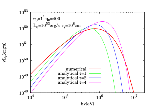
Figure 2.— Observed luminosity spectrum in the case of a uniform jet ($\theta_{0}=\theta_{1}=1^{\circ}$) with parameters of the fireball given by $L_{0}=L_{1}=10^{53}~{}{\rm erg/s}$, $\eta_{0}=\eta_{1}=400$ and $r_{\rm i}=10^{8}~{}{\rm cm}$. The spectrum corresponds to the case when the line of sight to the observer is aligned to the jet axis ($\theta_{\rm obs}=0^{\circ}$). The red line shows the numerical result. The green, blue and purple lines show the analytical estimates of photospheric emission derived from equation (18) for $r=r_{\rm ph}$, $r=r_{\rm ph}/2$ and $r=r_{\rm ph}/4$, respectively.

3.2. Stratified Jet

Here we show the results for a two-component stratified jet. In all cases, the half opening angle of the spine is fixed at $\theta_{0}=0.5^{\circ}$.

As mentioned in §3.1, when a uniform jet is assumed, spectra tend to be thermal-like with slight modifications from blackbodies originating from a sphere with radius $r=r_{\rm ph0}/5$. On the other hand, the appearance of the spectrum can deviate significantly from a thermal one when a strong velocity shear is present in the outflow, since photons which cross the shear flow multiple times can gain energy through a Fermi-like acceleration mechanism. This can be understood as follows. Under the assumption of elastic scattering, the energy gain of photons in a single scattering event can be expressed as

$$\frac{\nu_{\rm sc}}{\nu_{\rm in}}=\frac{1-\beta{\rm cos}\theta_{\rm in}}{1-\beta{\rm cos}\theta_{\rm sc}},$$ (19)

where $\nu_{\rm in}$ ($\nu_{\rm sc}$) and $\theta_{\rm in}$ ($\theta_{\rm sc}$) are the frequency and angle between the the fluid velocity and photon propagation direction before (after) the scattering, respectively. Hence, if $\theta_{\rm sc}<\theta_{\rm in}$, photons gain energy and vice versa. Photons which have crossed the boundary layer from the sheath to the spine region tend to gain energy when they are scattered there (upscatter). This is simply because the photons within the sheath region tend to have larger angle between their propagation direction and fluid velocity than those in the spine region. On the other hand, photon which have crossed the boundary layer from the spine to the sheath region tend to lose energy (downscatter) due to the same reason. Consequently, some fraction of photons which cross the boundary layer multiple times can gain energy, since the energy gain by the upscattering overcome the downscattering in average. This mechanism can give rise to a non-thermal spectrum at the high frequencies.

To obtain a rough estimation of the average energy gain and loss rate ($\nu_{\rm sc}/\nu_{\rm in}$) for each process, let us approximate the radially expanding spine and sheath regions as a plane parallel flow. Under the above consideration, the typical angle between the photon propagation direction and the fluid velocity direction for the photons in the spine (sheath) region can be roughly estimated as $\langle{\theta_{v}}\rangle_{0}\sim\Gamma_{0}^{-1}$ ($\langle{\theta_{v}}\rangle_{1}\sim\Gamma_{1}^{-1}$). Since the angle $\theta_{v}$ is conserved along the photon’s path in the case of a plane parallel flow, the typical energy gain rate by the upscattering in the spine region can be evaluated by substituting $\theta_{\rm in}=\langle{\theta_{v}}\rangle_{1}\sim\Gamma_{1}^{-1}$ and $\theta_{\rm sc}=\langle\theta_{v}\rangle_{0}\sim\Gamma_{0}^{-1}$ in equation (19) and is given as

$$\left\langle\frac{\nu_{\rm sc}}{\nu_{\rm in}}\right\rangle_{\rm up}\sim\frac{1-\beta_{0}{\rm cos}\langle{\theta_{v}}\rangle_{1}}{1-\beta_{0}{\rm cos}\langle{\theta_{v}}\rangle_{0}}\sim\frac{1}{2}\left\{1+\left(\frac{\Gamma_{0}}{\Gamma_{1}}\right)^{2}\right\}.$$ (20)

Similarly, the typical energy loss rate by the downscattering in the sheath region is given as

$$\left\langle\frac{\nu_{\rm sc}}{\nu_{\rm in}}\right\rangle_{\rm down}\sim\frac{1-\beta_{1}{\rm cos}\langle{\theta_{v}}\rangle_{0}}{1-\beta_{1}{\rm cos}\langle{\theta_{v}}\rangle_{1}}\sim\frac{1}{2}\left\{1+\left(\frac{\Gamma_{1}}{\Gamma_{0}}\right)^{2}\right\}.$$ (21)

From the above equations, it is clear that the energy gain by the upscattering overcomes the energy loss by the downscattering ($\langle\nu_{\rm sc}/\nu_{\rm in}\rangle_{\rm up}\langle\nu_{\rm sc}/\nu_{\rm in}\rangle_{\rm down}\sim(1/4)[2+(\Gamma_{0}/\Gamma_{1})^{2}+(\Gamma_{1}/\Gamma_{0})^{2}]>1$). It is also clear that the efficiency of the acceleration per each cycle of crossing $\langle\nu_{\rm sc}/\nu_{\rm in}\rangle_{\rm up}\langle\nu_{\rm sc}/\nu_{\rm in}\rangle_{\rm down}\sim(1/4)[2+(\Gamma_{0}/\Gamma_{1})^{2}+(\Gamma_{1}/\Gamma_{0})^{2}]$ is controlled by the ratio between the bulk Lorentz factor of the two regions $\Gamma_{0}/\Gamma_{1}$ and increases as the ratio becomes larger. It is worth noting that, while the average value of the energy ratio $\nu_{\rm sc}/\nu_{\rm in}$ roughly obeys the above equations, the dispersion around the average value is large, since it depends quite sensitively on the scattering angles ($\theta_{\rm in}$ and $\theta_{\rm sc}$; see Eq. (19)). When a photon from the sheath region that has an angle $\theta_{\rm in}=f_{1}\Gamma_{1}^{-1}$ is scattered in the spine region with an angle $\theta_{\rm sc}=f_{0}\Gamma_{0}^{-1}$, the energy gain by the scattering can be written as $\nu_{\rm sc}/\nu_{\rm in}\sim(1+f_{0}^{2})^{-1}[1+f_{1}^{2}(\Gamma_{0}/\Gamma_{1})^{2}]$. It is clear from the above equation that a small change in the scattering angles ($\theta_{\rm in}=\langle{\theta_{v}}\rangle_{0}\sim\Gamma_{0}^{-1}$ and $\theta_{\rm sc}=\langle{\theta_{v}}\rangle_{1}\sim\Gamma_{1}^{-1}$) leads to a quite large change in the energy ratio. For example, in the case of $f_{0}=0$ and $f_{1}=2$, the energy ratio due to the upscattering is larger than the typical value by a factor of $(\nu_{\rm sc}/\nu_{\rm in})(\langle\nu_{\rm sc}/\nu_{\rm in}\rangle_{\rm up})^{-1}\sim 2[1+4(\Gamma_{0}/\Gamma_{1})^{2}][1+(\Gamma_{0}/\Gamma_{1})^{2}]^{-1}\sim 8$. Note also that, once the photon energy (evaluated in the electron rest frame) approaches close to the electron rest mass energy $h\nu_{\rm cmf}\sim m_{e}c^{2}$, where $m_{e}$ is the electron rest mass, the scattering can no longer be approximated as elastic, since recoil effect becomes non-negligible (Klein-Nishina effect). In this case, the acceleration efficiency is significantly reduced.

In Fig. 3, we display the obtained result for the case of a stratified jet with $\eta_{0}=400$ and $L_{0}=10^{53}~{}{\rm erg/s}$ for the spine and $\eta_{1}=200$ and $L_{1}=(\eta_{1}/\eta_{0})L_{0}=5\times 10^{52}~{}{\rm erg/s}$ for the sheath. As mentioned in §2, the injection radius is set at a position where a velocity shear between the two regions develops ($r_{\rm inj}=r_{\rm s1}$). The corresponding optical depth is $\tau(r_{\rm inj})\sim 100$ for the spine and $\tau(r_{\rm inj})\sim 180$ for the sheath. The various lines in the figure show the cases for the observer angle with respect to the jet axis being $\theta_{\rm obs}=0^{\circ}$ (red), $0.25^{\circ}$ (green), $0.4^{\circ}$ (blue), $0.5^{\circ}$ (purple), $0.6^{\circ}$ (light blue) and $0.75^{\circ}$ (black). As we can see, the spectrum varies quite sensitively with the observer angle. The spectrum for $\theta_{\rm obs}=0^{\rm\circ}$ is thermal-like and nearly identical to that obtained in the case of a uniform jet (Fig. 2). The reason for this is simple. Since most of the scattered photons propagate in a direction within a cone of half opening angle $\sim 1/\Gamma\sim 0.14^{\circ}(\Gamma/400)^{-1}$, the majority of the observed photons are from a region of $\theta\lesssim 0.14^{\circ}$. Hence, only a small fraction of photons from the sheath region and the boundary ($\theta\geq\theta_{0}=0.5^{\circ}$) can reach the observer, so that the spectrum does not deviate largely from the case of uniform jet. On the other hand, if the observer angle is larger, photons from the sheath and boundary layer become observable. As a result, a non-thermal component appears above the peak energy of the thermal spectrum due to the photon acceleration in the boundary layer. The non-thermal component is hardest when the observer angle is aligned to the boundary layer $\theta_{\rm obs}=\theta_{0}=0.5^{\circ}$ and becomes softer as the deviation between $\theta_{\rm obs}$ and $\theta_{0}$ becomes larger, simply because the boundary layer corresponds to the site of photon acceleration. As mentioned earlier, the photon acceleration becomes inefficient when the photon energy becomes large enough so that the recoil of electrons cannot be neglected (Klein-Nishina effect). Hence, in all cases, the spectrum does not extend up to energies higher than $h\nu\sim\Gamma_{0}m_{e}c^{2}\sim 200(\Gamma_{0}/400)~{}{\rm MeV}$.

Note also that the peak energy and the luminosity of the thermal component differs enormously for $\theta_{\rm obs}>\theta_{0}$ and for $\theta_{\rm obs}<\theta_{0}$, due to the differences in the assumed parameters in the spine and sheath regions. For an observer at $\theta_{\rm obs}<\theta_{0}$, the thermal component is determined mainly by photons which have propagated through the spine region. Therefore, the observed spectrum is nearly identical to the case of the uniform jet considered above in which a same set of parameters ($\eta_{0}$, $L_{0}$ and $r_{\rm i}$) is assumed. On the other hand, for an observer at $\theta_{\rm obs}>\theta_{0}$, photons which have propagated through the sheath region dominate the thermal component. Accordingly, the peak energy and luminosity are lower by a factor $\sim(\eta_{0}/\eta_{1})^{8/3}(L_{0}/L_{1})^{-5/12}\sim 4.7$ and $\sim(\eta_{0}/\eta_{1})^{8/3}(L_{0}/L_{1})^{1/3}\sim 8$, respectively.

In Fig. 4, we display the results obtained for $\eta_{0}=200$ and $L_{0}=10^{52}~{}{\rm erg/s}$ for the spine and $\eta_{1}=100$ and $L_{0}=5\times 10^{51}~{}{\rm erg/s}$ for the sheath. That is, the terminal Lorentz factor of the outflow is smaller by a factor of $2$ for both the spine and the sheath than those assumed in the previous case. The optical depths at the injection radius are $\tau(r_{\rm inj})\sim 170$ for the spine and $\tau(r_{\rm inj})\sim 290$ for the sheath. As in the previous case, the non-thermal component is hardest when $\theta_{\rm obs}=\theta_{0}=0.5^{\circ}$ and becomes softer as the deviation between $\theta_{\rm obs}$ and $\theta_{0}$ becomes larger. However, the major difference with the previous case is that the observer dependence of the hardness is weaker. For example, as shown in Fig. 4, the non-thermal component can be prominent even for $\theta_{\rm obs}=0^{\circ}$. This is because beaming effect is weaker than the previous case due to the smaller values of the Lorentz factor, so that the photons can spread out in wider angles.

The dependence of the spectrum on the difference between the dimensionless entropies (terminal Lorentz factor) of the spine and sheath is displayed in Fig. 5. Each panel corresponds to the result for the observer angle fixed at $\theta_{\rm obs}=0.25^{\circ}$ (top panel), $\theta_{\rm obs}=0.4^{\circ}$ (middle left), $\theta_{\rm obs}=0.5^{\circ}$ (middle right), $\theta_{\rm obs}=0.6^{\circ}$ (bottom left) and $\theta_{\rm obs}=0.75^{\circ}$ (bottom right). In all cases, the dimensionless entropy and kinetic luminosity of the spine are chosen to be $\eta_{0}=400$ and $L_{0}=10^{53}~{}{\rm erg/s}$, respectively. The red line shows the case for a uniform jet, while the green, blue, purple, light blue and black lines show the cases for a sheath with dimensionless entropies of $\eta_{1}=300$, $\eta_{1}=250$, $\eta_{1}=200$, $\eta_{1}=150$ and $\eta_{1}=100$, respectively. The kinetic luminosity of the sheath is determined by $L_{1}=(\eta_{0}/\eta_{1})L_{0}$.

As mentioned earlier, the peak energy and luminosity of the thermal-component depend on the dimensionless entropy and the kinetic luminosity as $E_{\rm p}\propto\eta^{8/3}L^{-5/12}$ and luminosity $L_{\rm p}\propto\eta^{8/3}L^{1/3}$. Hence, for observer mainly seeing the photons from the sheath region ($\theta_{\rm obs}>\theta_{0}$), these values show considerable decrease in models assuming smaller $\eta_{1}$ as is seen in the figure. The non-thermal component becomes significant as $\eta_{1}$ becomes smaller. This tendency is due to the following reasons. One is simply because the bulk Lorentz factor of the sheath becomes smaller for smaller $\eta_{1}$. As a result, the ratio between the bulk Lorentz factor of the spine and sheath $\Gamma_{0}/\Gamma_{1}$ becomes larger which in turn leads to an increase in the energy gain per each crossing as explained earlier in this section. In addition, the wider spreading of the photons propagating in the sheath region due to the increase in the beaming angle $\sim\Gamma_{1}^{-1}$ increases the chance for the photons to cross the boundary layer from the sheath to the spine region. Another reason is that, for smaller value of $\eta_{1}$, the radius where the velocity shear begins to develop $r_{\rm s1}=\eta_{1}r_{\rm i}$ becomes smaller. This also leads to an increase in the probability for the photons to be accelerated, since the optical depth of the acceleration region ($r>r_{\rm s1}$) increases (see equation (7)).

3.3. Relation Between Photon Energy and Number of Crossings

To demonstrate that photons accelerated via the multiple crossing of the spine and sheath boundary layer are indeed the origin of the non-thermal component, we analyzed the relation between the photon energy and the number of crossings that the corresponding photons have experienced. Here the number of crossings, $n_{\rm cr}$, is defined as the total number of events that the photon has crossed the boundary layer (either from spine to sheath or sheath to spine) before it reaches the outer boundary $r_{\rm out}$.

In Fig. 6, we show the distribution of the average number of crossings for a given observed photon energy, $\langle n_{\rm cr}\rangle_{\nu}$. On the other hand, distribution of the average observed energy for a given number of crossings, $\langle\nu\rangle_{n_{\rm cr}}$, is displayed in Fig. 7. The two cases of stratified jet that are displayed in the figures by the purple (Case I: $\eta_{0}=400$ and $\eta_{1}=200$) and black lines (Case II: $\eta_{0}=400$ and $\eta_{1}=100$) correspond to the analysis of photons shown in Fig. 5 using same colors.

From Fig. 6, it is confirmed that the photons at higher energies tend to have larger number of crossings. While the photons below the thermal peak energy ($h\nu\lesssim~{}{\rm MeV}$) do not require multiple crossings, the prominent non-thermal component extending above $\sim 1~{}{\rm MeV}$ is produced by the photons that cross the boundary layer $\sim 10-15$ times in average. Comparing the two cases, the overall distribution of $\langle n_{\rm cr}\rangle_{\nu}$. does not vary much. The difference in the average number of crossing is within $\sim 2$ in all energies up to $\sim 100~{}{\rm MeV}$. Note that, however, that this does not imply that the average energy for a given number of crossings $\langle\nu\rangle_{n_{\rm cr}}$ does not vary much in the two cases. Conversely, the difference in $\langle\nu\rangle_{n_{\rm cr}}$ is quite large between the two cases as is seen in Fig. 7, since the average energy gain per crossing is quite sensitive to the ratio in the terminal Lorentz factor $\Gamma_{0}/\Gamma_{1}$ (see Eqs. (20) and (21)). However, due to the large dispersion in the energy gain per crossing, the energy distribution of photons does not show a sharp peak at the average energy $\langle\nu\rangle_{n_{\rm cr}}$ but extends to energies below and above $\langle\nu\rangle_{n_{\rm cr}}$ by many orders of magnitude. As a result, the distribution of $\langle n_{\rm cr}\rangle_{\nu}$ do not directly reflect the distribution of $\langle\nu\rangle_{n_{\rm cr}}$, since the photons which have crossed the boundary layer a certain number of times can dominate over the other population of photons in wide energy ranges. To clarify this, we show the energy distribution of the photon number count rate, $\nu N_{\nu}$ [photons/s], for a given number of crossings in 8. From the figure, it is confirmed that, while there is a significant discrepancy in $\langle\nu\rangle_{n_{\rm cr}}$, the photons with number of crossing $n_{\rm cr}\sim 10$ tend to dominate the population in the energy range in which non-thermal component becomes prominent ($h\nu\gtrsim{\rm few}~{}{\rm MeV}$) in both cases. For this reason, the resultant distribution of $\langle n_{\rm cr}\rangle_{n_{\rm cr}}$ does not vary much in the two cases.

Regarding the distribution of the average energy, $\langle\nu\rangle_{n_{\rm cr}}$ tends to increase with the increasing number of crossing $n_{\rm cr}$ initially and then approaches a constant value. This asymptotic behaviour is due to the Klein-Nishina effect. As the photon energy becomes large and exceeds $100~{}{keV}$ in the comoving frame, acceleration efficiency is reduced by the effect (see §3.2 for detail), and the average energy can no longer increase. As in seen in Fig. 7, the dependence of $\langle\nu\rangle_{n_{\rm cr}}$ on $n_{\rm cr}$ is not smooth but rather bumpy. This reflects the fact that the photons tend to be upscattered when crossing from the sheath to spine region occurs (see Eq. (20)), while, on the other hand, tend to be downscattered when crossing in the opposite direction occurs (see Eq. (21)). Therefore, the energy of individual photons is not a monotonically increasing function of $n_{\rm cr}$ but shows a bumpy dependence, since upscattering and downscattering occurs alternately in each crossing events. Although somewhat reduced, this feature remains even after averaging up and leads to the appearance wiggles in the distribution of $\langle\nu\rangle_{n_{\rm cr}}$.

To quantify the energy gain and loss in each crossing, we display the ratio of the average energy for photons with $n_{\rm cr}$ crossings to that for photons with $n_{\rm cr}-1$ crossings ($\langle\nu\rangle_{n_{\rm cr}}/\langle\nu\rangle_{n_{\rm cr}-1}$) in Fig. 9. In addition to the analysis of the total photons, we also display the results of the analysis for the two populations of photons that were initially injected in the spine region ($\theta_{\rm inj}\leq\theta_{0}$; blue line) and sheath regions ($\theta_{\rm inj}>\theta_{0}$; green line). In the former case ($\theta_{\rm inj}\leq\theta_{0}$), if $n_{\rm cr}$ is an odd (even) number, the number of crossings from the spine (sheath) to sheath (spine) region is greater by $1$ than that for $n_{\rm cr}-1$ crossings. Hence, the number of downscattering (upscattering) event is greater by $1$ for the photons with an odd (even) number of $n_{\rm cr}$ than for those with $n_{\rm cr}-1$ crossings. As a result, $\langle\nu\rangle_{n_{\rm cr}}/\langle\nu\rangle_{n_{\rm cr}-1}$ is less (greater) than unity for the odd (even) number of $n_{\rm cr}$. On the other hand, as is obvious, the opposite is true for the latter case ($\theta_{\rm inj}>\theta_{0}$). Jets with a larger difference in the terminal Lorentz factor (Case II; right panel) show a larger range of energy ratio $\langle\nu\rangle_{n_{\rm cr}}/\langle\nu\rangle_{n_{\rm cr}-1}$ than those with a smaller difference (Case I; left panel), since the efficiency of the single upscattering (downscattering) increases (decreases) as the relative difference in the Lorentz factor becomes larger.

Regarding the upscatterings, the energy ratio $\langle\nu\rangle_{n_{\rm cr}}/\langle\nu\rangle_{n_{\rm cr}-1}$ for photons that cross the boundary from the sheath to spine region (green line) only once ($n_{\rm cr}=1$) is relatively small because a large fraction of these photons experience the crossing when the velocity shear is not fully developed ($r<r_{\rm s0}$). For photons with a larger number of crossings ($n_{\rm cr}\gtrsim 2$), a large fraction of the photons experience the last crossing at $r>r_{\rm s0}$, where the velocity shear is fully developed. Therefore, the energy ratio is larger than that for $n_{\rm cr}=1$ and is roughly constant as long as the Klein-Nishina effect is negligible. When the Klein-Nishina effect becomes important ($n_{\rm cr}\gtrsim 10$ for Case I and $n_{\rm cr}\gtrsim 5$ for Case II), $\langle\nu\rangle_{n_{\rm cr}}/\langle\nu\rangle_{n_{\rm cr}-1}$ decreases as $n_{\rm cr}$ increases, and again asymptotically approaches a constant value. On the other hand, regarding the case of downscatterings, the energy ratio is relatively insensitive to the number of crossings in both cases and is roughly in the range $\sim 0.25-0.6$. It is worth noting that the values of energy ratio are consistent within a factor of $\sim 2$ with the rough estimations given by Eqs. (20) and (21). Above the saturation radius ($r\geq r_{\rm s0}$), the equations predict an upscattering (downscattering) with energy ratio of $\sim 2.5$ ($\sim 0.6$) and $\sim 8.5$ ($\sim 0.5$) for Cases I and II, respectively. The energy ratio of the total photons is larger and smaller when the photons from the spine correspond to the upscattering (even $n_{\rm cr}$) and downscattering (even $n_{\rm cr}$), respectively, since more photons originate from the spine region than from the sheath region.

Lastly, to obtain a further insight into the relation between the photon acceleration and number of crossing, we show the evolution of the average photon energy evaluated in the comoving frame, $\nu_{\rm cmf}$, with radius in Fig 10. The red, green, blue, purple, light blue, yellow and black lines display the photons that have experienced $n_{\rm cr}=0$, $3$, $5$, $10$, $15$, $20$ and $25$ crossings, respectively. For comparison, we also plot the curve of $\nu_{\rm cmf}\propto r^{-2/3}$ with a thin black line, which corresponds to the adiabatic cooling expected above the saturation radius ($r\geq r_{\rm s0}$).

Regarding the photons that do not experience any crossings ($n_{\rm cr}=0$), the overall evolution of the energy is determined solely by the adiabatic cooling due to the expansion of the jet, since photon acceleration does not take place. Below the saturation radius of the spine $r\leq r_{\rm s0}$, the cooling rate in the spine region ($\nu_{\rm cmf}\propto r^{-1}$) is higher than that in the sheath region ($\nu_{\rm cmf}\propto r^{-2/3}$), since the spine region is in the acceleration phase, while the sheath region is in the coasting phase ($r\geq r_{\rm s1}$). Hence, the energy evolution of the average comoving energy is in between the two cooling rates. At larger radii ($r\geq r_{\rm s0}$), since both regions are in the coasting phase, the average energy evolves as $\nu_{\rm cmf}\propto r^{-2/3}$ until the coupling between the photon and matter becomes weak ($r\lesssim 0.1r_{\rm ph0}$). The cooling rate gradually reduces at $r\gtrsim 0.1r_{\rm ph0}$ due to the weak coupling, and the comoving energy approaches a constant value. It is worth noting that the behaviour of the average comoving energy for photons above the saturation radius is consistent with that found in the previous studies (e.g., Pe’er, 2008; Beloborodov, 2011; Bégué et al., 2013).

Regarding the photons with at least one crossing ($n_{\rm cr}\geq 1$), the evolution of the comoving energy cannot be described only by the adiabatic cooling due to the presence of the photon acceleration. As the number of the crossings increases, the departure from the simple adiabatic cooling becomes significant and the comoving energies tend to be larger. For a given number of crossings, the departure is more prominent in Case II than in Case I due to the increase in the acceleration efficiencies. When the number of the crossings is sufficiently large so that the effect of Klein-Nishina becomes non-negligible, the evolution of the average comoving energy asymptotically approaches a single curve since the acceleration saturates. This tendency is clearly seen in Fig. 10 (for example, see lines that display the evolution of photons with $n_{\rm cr}\geq 10$ in Case II).

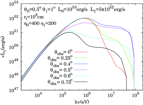
Figure 3.— Observed luminosity spectrum in the case of spine-sheath jet in which the spine jet with half opening angle of $\theta_{0}=0.5^{\circ}$ is embedded in a wider sheath outflow with half opening angle of $\theta_{1}=1^{\circ}$. The employed values for dimensionless entropy (terminal Lorentz factor) and kinetic luminosity are chosen as $\eta_{0}=400$ and $L_{0}=10^{53}~{}{\rm erg/s}$ for the spine and $\eta_{1}=200$ and $L_{1}=(\eta_{1}/\eta_{0})L_{0}=5\times 10^{52}~{}{\rm erg/s}$ for the sheath, respectively. The initial radius of fireball is chosen as $r_{\rm i}=10^{8}~{}{\rm cm}$ in both regions. The various lines show the cases where the observer angle with respect to the jet axis is $\theta_{\rm obs}=0^{\circ}$ (red), $0.25^{\circ}$ (green), $0.4^{\circ}$ (blue), $0.5^{\circ}$ (purple), $0.6^{\circ}$ (light blue) and $0.75^{\circ}$ (black).

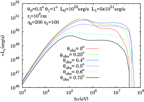
Figure 4.— Same as Fig.3, but for $\eta_{0}=200$, $\eta_{1}=100$, $L_{0}=10^{52}~{}{\rm erg/s}$ and $L_{0}=5\times 10^{51}~{}{\rm erg/s}$.

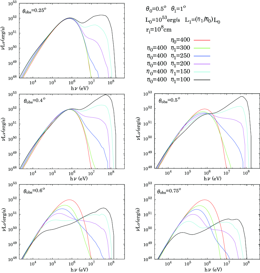
Figure 5.— Observed luminosity spectrum for a uniform jet and a spine-sheath jet in which the spine jet with half opening angle of $\theta_{0}=0.5^{\circ}$ is embedded in a wider sheath outflow with half opening angle of $\theta_{1}=1^{\circ}$. Each panel shows a different observer angle fixed at $\theta_{\rm obs}=0.25^{\circ}$ (top panel), $\theta_{\rm obs}=0.4^{\circ}$ (middle left), $\theta_{\rm obs}=0.5^{\circ}$ (middle right), $\theta_{\rm obs}=0.6^{\circ}$ (bottom left) and $\theta_{\rm obs}=0.75^{\circ}$ (bottom right). The employed values for dimensionless entropy (terminal Lorentz factor) and kinetic luminosity are chosen as $\eta_{0}=400$ and $L_{0}=10^{53}~{}{\rm erg/s}$ for the spine. The red line shows the case of a uniform jet, while the green, blue, purple, light blue and black show the cases for the dimensionless entropy of the sheath given by $\eta_{1}=300$, $\eta_{1}=250$, $\eta_{1}=200$, $\eta_{1}=150$ and $\eta_{1}=100$, respectively. In each case, the kinetic luminosity of the sheath is given by $L_{1}=(\eta_{0}/\eta_{1})L_{0}$.

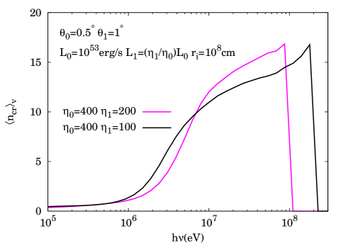
Figure 6.— Average number of crossing events of the spine-sheath boundary layer as a function of observed photon energy for a jet in which the spine region with half opening angle of $\theta_{0}=0.5^{\circ}$ is embedded in a wider sheath outflow with half opening angle of $\theta_{1}=1^{\circ}$. The employed values for dimensionless entropy (terminal Lorentz factor) and kinetic luminosity are chosen as $\eta_{0}=400$ and $L_{0}=10^{53}~{}{\rm erg/s}$ for the spine. The purple and black lines show the cases of the dimensionless entropy of the sheath given by $\eta_{1}=200$ and $\eta_{1}=100$, respectively. In each case, the kinetic luminosity of the sheath is given by $L_{1}=(\eta_{0}/\eta_{1})L_{0}$.

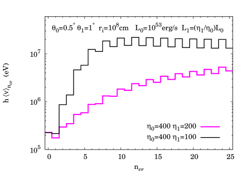
Figure 7.— Average energy of the photons as a function of the number of crossings of the spine-sheath boundary layer $n_{\rm cr}$ for a jet in which the spine region with half opening angle of $\theta_{0}=0.5^{\circ}$ is embedded in a wider sheath outflow with half opening angle of $\theta_{1}=1^{\circ}$. The employed values for dimensionless entropy (terminal Lorentz factor) and kinetic luminosity are chosen as $\eta_{0}=400$ and $L_{0}=10^{53}~{}{\rm erg/s}$ for the spine. The purple and black lines show the cases of the dimensionless entropy of the sheath given by $\eta_{1}=200$ and $\eta_{1}=100$, respectively. In each case, the kinetic luminosity of the sheath is given by $L_{1}=(\eta_{0}/\eta_{1})L_{0}$.

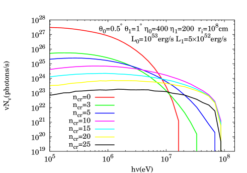
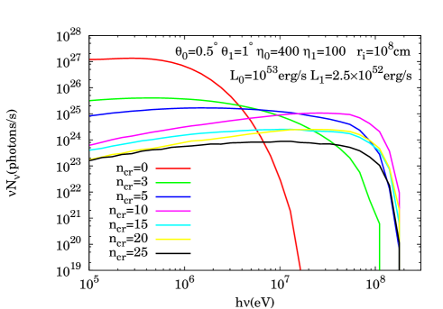
Figure 8.— Energy distribution of photons for a given number of crossing events in the case of jet in which a spine region with half opening angle of $\theta_{0}=0.5^{\circ}$ is embedded in a wider sheath outflow with half opening angle of $\theta_{1}=1^{\circ}$. The red, green, blue, purple, light blue, yellow and black lines display the photons that have experienced $n_{\rm cr}=0$, $3$, $5$, $10$, $15$, $20$ and $25$ crossings, respectively. The employed values for dimensionless entropy (terminal Lorentz factor) and kinetic luminosity are chosen as $\eta_{0}=400$ and $L_{0}=10^{53}~{}{\rm erg/s}$ for the spine. The left and right panels show the cases where the dimensionless entropy of the sheath is given by $\eta_{1}=200$ and $\eta_{1}=100$, respectively. In each case, the kinetic luminosity of the sheath is given by $L_{1}=(\eta_{0}/\eta_{1})L_{0}$.

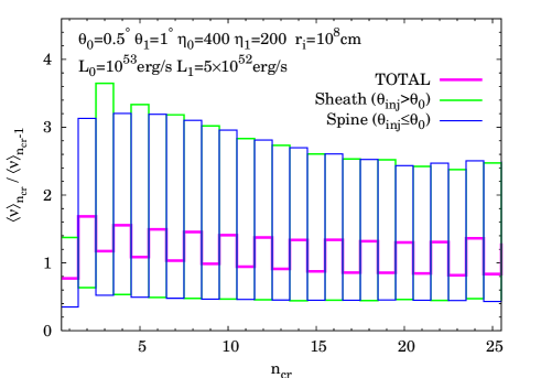
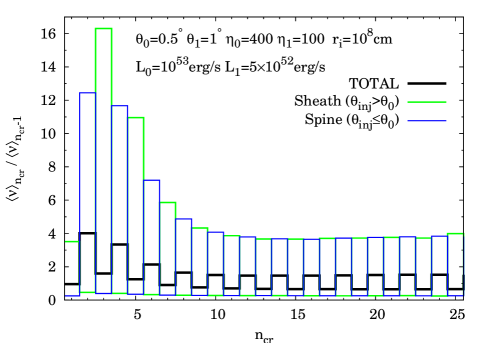
Figure 9.— Ratio of the average observed energy for photons which cross the spine-sheath boundary layer ($\theta=\theta_{0}$) $n_{\rm cr}$ times to those which experience $n_{\rm cr}-1$ crossings for a jet in which a spine region with half opening angle of $\theta_{0}=0.5^{\circ}$ is embedded in a wider sheath outflow with half opening angle of $\theta_{1}=1^{\circ}$. The employed values for dimensionless entropy (terminal Lorentz factor) and kinetic luminosity are chosen as $\eta_{0}=400$ and $L_{0}=10^{53}~{}{\rm erg/s}$ for the spine. The left and right panels show the cases of the dimensionless entropy of the sheath given by $\eta_{1}=200$ and $\eta_{1}=100$, respectively. In each case, the kinetic luminosity of the sheath is given by $L_{1}=(\eta_{0}/\eta_{1})L_{0}$. The energy ratio for total photons are displayed in the left and right panels with the purple and black lines, respectively. In addition, also the energy ratio for the photons that were initially injected in the spine region ($\theta_{\rm inj}\leq\theta_{0}$) and sheath region ($\theta_{\rm inj}>\theta_{0}$) are shown by blue and green lines, respectively, in both panels.

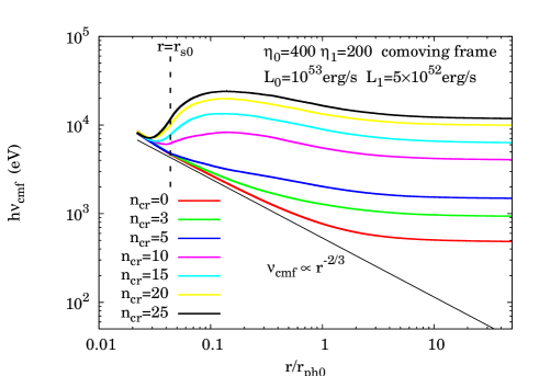
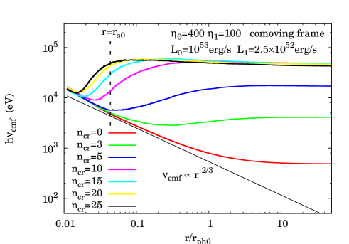
Figure 10.— Average comoving energy of photons as a function of radius for a jet in which a spine region with half opening angle of $\theta_{0}=0.5^{\circ}$ is embedded in a wider sheath outflow with half opening angle of $\theta_{1}=1^{\circ}$. The red, green, blue, purple, light blue, yellow and black lines display the photons that have experienced $n_{\rm cr}=0$, $3$, $5$, $10$, $15$, $20$ and $25$ crossings, respectively. The thin black solid line plots the curve of $\propto r^{-2/3}$, which corresponds to the adiabatic cooling expected above the saturation radius ($r\geq r_{\rm s0}$). The employed values for dimensionless entropy (terminal Lorentz factor) and kinetic luminosity are chosen as $\eta_{0}=400$ and $L_{0}=10^{53}~{}{\rm erg/s}$ for the spine. The left and right panels show the cases of the dimensionless entropy of the sheath given by $\eta_{1}=200$ and $\eta_{1}=100$, respectively. In each case, the kinetic luminosity of the sheath is given by $L_{1}=(\eta_{0}/\eta_{1})L_{0}$.

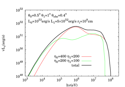
Figure 11.— Observed luminosity spectrum in the case of spine-sheath jet in which a spine jet with half opening angle of $\theta_{0}=0.5^{\circ}$ is embedded in a wider sheath outflow with half opening angle of $\theta_{1}=1^{\circ}$. The observer angle is fixed as $\theta_{\rm obs}=0.4^{\circ}$. The black solid line shows the overall spectrum for the case when the dimensionless entropy of the spine-sheath jet have evolved from $\eta_{0}=400$ and $\eta_{1}=200$ (initial stage) to $\eta_{0}=200$ and $\eta_{1}=100$ (later stage), while the kinetic luminosity is fixed as $L_{0}=10^{53}~{}{\rm erg/s}$ and $L_{1}=5\times 10^{52}~{}{\rm erg/s}$. The red and green solid lines show the contribution from the initial and later stages, respectively.

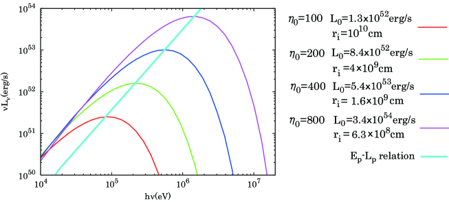
Figure 12.— Observed spectra in the case of a uniform jet that reproduces the observed $E_{\rm p}-L_{\rm p}$ relation and radiative efficiency of $\eta_{\gamma}\sim 0.2$. The red, green, blue, purple lines correspond to the cases of $\eta_{0}=100$, $\eta_{0}=200$, $\eta_{0}=400$ and $\eta_{0}=500$. The thick light blue line displays the observed $E_{\rm p}$-$L_{\rm p}$ relation.

4. DISCUSSIONS

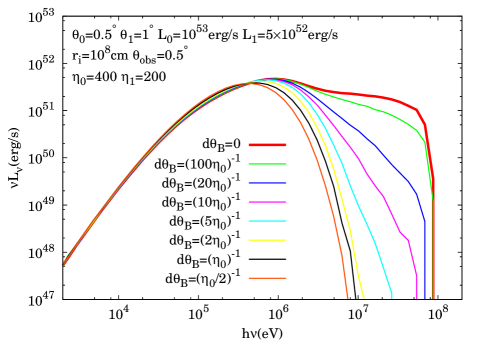
Figure 13.— Observed luminosity spectrum for a spine-sheath jet in which the width of the boundary layer $d\theta_{\rm B}$ is taken to be non-zero. The the spine and sheath regions are located in the transverse range $0\leq\theta\leq\theta_{\rm i}=\theta_{0}-d\theta_{\rm B}/2$ and $\theta_{\rm ii}=\theta_{0}+d\theta_{\rm B}/2\leq\theta\leq\theta_{1}$, respectively. In all cases, fixed values of $\theta_{0}=0.5^{\circ}$ and $\theta_{1}=1^{\circ}$ are employed and the observer angle is fixed at the midpoint of the boundary layer $\theta_{\rm obs}=\theta_{0}=0.5^{\circ}$. The employed values for dimensionless entropy (terminal Lorentz factor) and kinetic luminosity are chosen as $\eta_{0}=400$ and $L_{0}=10^{53}~{}{\rm erg/s}$ for the spine and $\eta_{0}=200$ and $L_{0}=5\times 10^{52}~{}{\rm erg/s}$ for the sheath. While the thick red line displays the case for an infinitesimal width ($d\theta_{\rm B}=0$), the thin green, blue, purple, light blue, yellow, black and red lines display the cases for widths of $d\theta_{\rm B}=(100\eta_{0})^{-1}$, $(20\eta_{0})^{-1}$, $(10\eta_{0})^{-1}$, $(5\eta_{0})^{-1}$, $(2\eta_{0})^{-1}$, $\eta_{0}^{-1}$ and $(\eta_{0}/2)^{-1}$, respectively.

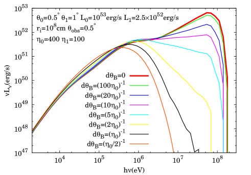
Figure 14.— Same as Fig.13, but for $\eta_{1}=100$, $L_{1}=2.5\times 10^{52}~{}{\rm erg/s}$.

4.1. Comparison with Observations

So far, we have shown that in the presence of velocity shear, photons can be accelerated at the shear region producing a high energy power-law component above the thermal peak energy. From observations, the observed spectra of GRB prompt emission can be often modeled by a Band function, which is a smoothly joined broken power-law that peaks at $\sim$ a few $100~{}{\rm keV}$. The photon indices below and above the peak ($\alpha_{\rm ph}$ and $\beta_{\rm ph}$) vary from source to source ($\nu L_{\nu}\propto\nu^{\alpha_{\rm ph}+2}$ for $\nu<\nu_{\rm p}$ and $\nu L_{\nu}\propto\nu^{\beta_{\rm ph}+2}$ for $\nu>\nu_{\rm p}$). Focusing on the high-energy slope $\beta_{\rm ph}$, the measured values are roughly in the range between $-2$ and $-3$, with a typical value at $\sim-2.5$. The power-law component predicted in our model can accommodate various spectral indices depending on the flow parameters as well as observer angle. Hence, by adopting appropriate values for our parameter set, the observed high energy spectral slope ($\nu L_{\nu}\propto\nu^{-0.5\pm 0.5}$) as well as the harder and softer slopes observed in some GRBs can be reproduced as shown in Figs. 3-5.

Interestingly, our model can also reproduce spectral features seen in some peculiar GRBs such as GRB 090510(Ackermann et al., 2010), 090902B(Abdo et al., 2009) and 090926A(Ackermann et al., 2011). In these bursts, in addition to a Band-type (or thermal-like) component, an extra hard power-law component (photon index larger than $-2$) is required to model the overall spectrum. As shown in Fig. 5, in some cases, especially when the difference between $\eta_{0}$ and $\eta_{1}$ is large, the non-thermal power-law component does not join the thermal component smoothly at the peak energy, but appears as a hard power-law component which becomes prominent at energies above the bump of the thermal component. These spectral features resemble those found in these bursts. Hence, we emphasize that the spectra of peculiar bursts may be due to the relatively large difference in $\eta$ (or bulk Lorentz factor) in the shear region. It is noted, however, that the extra power-law component that also extends to energies below the thermal-like component found in GRB 090902B and 090510 is hard to explain. If present, different emission components such as synchrotron emission as discussed in Pe’er et al. (2012) may be required in order to explain the low energy end of the power-law component. We also note that, in order to extend the power-law component up to ${\rm GeV}$ energies, quite large Lorentz factors are required, since the non-thermal component extends only up to energy of $h\nu\lesssim 200(\eta/400)~{}{\rm MeV}$ due to the Klein-Nishina effect. A detailed discussion on this issue is given in §4.6.

On the other hand, the spectral slope below the peak energy is only moderately sensitive to the values of the parameters and can be well approximated by a blackbody emission from the off-axis region ($|\theta-\theta_{\rm obs}|\gtrsim\Gamma^{-1}$) of a sphere at a radius $r\sim r_{\rm ph}/5$ as in the case of a uniform jet. In all cases, the low energy photon indices are roughly $\alpha_{\rm ph}\sim 0.5$ which is harder than the typical observed value ($\alpha_{\rm ph}\sim-1$). It is noted, however, that this does not imply that the low energy slope cannot be reproduced within this scenario. For instance, while the instantaneous spectrum is hard, the time integration can lead to a softer spectrum if the evolution history of the outflow is considered. To demonstrate this, let us consider the case when the dimensionless entropies of the spine-sheath jet have evolved from $\eta_{0}=400$ and $\eta_{1}=200$ (initial stage) to $\eta_{0}=200$ and $\eta_{1}=100$ (later stage), while the kinetic luminosity is fixed as $L_{0}=10^{53}~{}{\rm erg/s}$ and $L_{1}=5\times 10^{52}~{}{\rm erg/s}$. We illustrate the resultant spectrum in Fig. 11 under the assumption that a nearly equal time period is spent in the two stages. The black solid line shows the overall spectrum, and the red and green solid lines show the contribution from the initial and later stages, respectively. Since the peak energy and the luminosity vary with the dimensionless entropy of the flow roughly as $\propto\eta^{8/3}$, they are smaller by a factor $\sim 6$, in the later stage. As a result, while the peak energy and luminosity of the overall spectra is determined by the initial stage, at lower energies, contribution from the later stage becomes dominant. Due to the superposition of the two components, the spectrum below the peak becomes softer than that of the individual component, so that a typical observed spectrum ($\nu L_{\nu}\propto\nu$) is reproduced. Note also that the high energy part of the overall spectrum largely resembles typical ones from observations. Hence, we conclude that typical observed spectra can be successfully reproduced when a time evolution is considered.

4.2. On the Observer Angle Dependence and Structure of the Jet

As shown in the previous section, our results have a quite strong dependence on the observer angle $\theta_{\rm obs}$. While strong non-thermal emission can be seen when the observer angle is close to the angle in which a velocity shear is present ($|\theta_{0}-\theta_{\rm obs}|\lesssim\Gamma^{-1}$), the non-thermal feature tends to be weaker for observer angles far from $\theta_{0}$. This tendency seems to contradict the fact that most of the observed GRBs have non-thermal features in their spectra. However, we emphasize that this difficulty can be overcome if the jet possesses a more complex structure. For example, if the jet has more than two components and velocity shear is present at multiple angles more closely spaced than $\Gamma^{-1}$, photons from the acceleration regions will be prominent for all observers lying within the opening angle of the jet ($\theta_{\rm obs}\leq\theta_{1}$). Even in the case of a simple spine-sheath jet, if the angular boundary of the spine and sheath ($\theta_{0}$) varied rapidly with time, the accelerated non-thermal photons would be observable across a broad range of angles. It should be also noted that the structure need not be in the direction of $\theta$. Strong velocity shear in the azimuthal ($\phi$) direction and/or radial direction due to the presence of turbulence or shocks can also provide an acceleration sites for the photons (Bromberg et al., 2011; Ioka et al., 2011). Any structure showing strong velocity shear within an angle $\Gamma^{-1}$ from the line-of-sight can give rise to a non-thermal component above the thermal peak. Hence, it is expected that jet having a rich structure and/or rapid time variability will be naturally accompanied by non-thermal emission, irrespective of the observer angle. The origin of the structure and variability could be due to the nature of the central engine (McKinney, 2006; Nagataki et al., 2007; Nagataki, 2009; McKinney & Blandford, 2009; Nagataki, 2011) and/or the propagation of jet through the envelope of the progenitor star (Zhang et al., 2003; Mizuta et al., 2006; Morsony et al., 2007; Lazzati et al., 2009; Mizuta et al., 2011; Nagakura et al., 2011).

4.3. On the $E_{\rm p}$-$L_{\rm p}$ relation

Our calculations have shown that the peak energy of the observed spectra can be roughly approximated as the thermal peak of a blackbody emission from the surface of optical depth $\tau(r)\sim 2$ ($r\sim r_{\rm ph}/2$). On the other hand, the peak luminosity shows rough agreement with that of the emission from $\tau(r)\sim 1$ ($r\sim r_{\rm ph}$). This result is valid for an adiabatic fireball which has a photosphere above the saturation radius ($r_{\rm ph}>r_{\rm s}$) (see §3.1 for detail). As a result, the peak energy and luminosity are given by

$$E_{\rm p}\sim 800r_{\rm i,8}^{1/6}\eta_{400}^{8/3}L_{53}^{-5/12}~{}{\rm keV},$$ (22)

and

$$L_{\rm p}\sim 10^{52}r_{\rm i,8}^{2/3}\eta_{400}^{8/3}L_{53}^{1/3}~{}{\rm erg/s},$$ (23)

respectively . Derived from observations, there is an empirical relation between the peak energy and luminosity (Yonetoku et al., 2004; Kodama et al., 2008; Nava et al., 2011; Amati et al., 2002; Wei & Gao, 2003) that is roughly given by

$$E_{\rm p}\approx 600\left(\frac{L_{\rm p}}{10^{53}~{}{\rm erg/s}}\right)^{1/2}~{}{\rm keV}.$$ (24)

Therefore, in order to reproduce the empirical relation from the photospheric emission, the parameters of the fireball ($r_{\rm i}$, $\eta$, and $L$) must satisfy

$$L_{53}\sim 12r_{\rm i,8}^{-2/7}\eta_{400}^{16/7}~{}{\rm erg/s}.$$ (25)

Another important ingredient for comparison with observations is the emission efficiency $\eta_{\gamma}=L_{\rm p}/L$. Observations of the afterglows suggest a quite high GRB efficiency in the range $0.01\lesssim\eta_{\gamma}\lesssim 1$, with a typical value at $\eta_{\gamma}\sim 0.1-0.2$ (e.g., Fan & Piran, 2006; Zhang et al., 2007). This gives another constraint on the fireball parameters which can be written as

$$0.01\lesssim 0.1r_{\rm i,8}^{2/3}\eta_{400}^{8/3}L_{53}^{-2/3}\lesssim 1.$$ (26)

To sum up, the observed $E_{\rm p}$-$L_{\rm p}$ relation as well as the high efficiency can be reproduced when equations (25) and (26) are satisfied.

In Fig. 12, we show the calculated spectra for a uniform jet ($\theta_{1}=\theta_{0}=1^{\circ}$) in which both conditions are fulfilled. The adopted values of the parameters are summarized in the figure. The red, green, blue and purple lines correspond to the cases of $\eta_{0}=100$, $\eta_{0}=200$, $\eta_{0}=400$ and $\eta_{0}=500$, respectively. The remaining parameters ($L_{0}$ and $r_{\rm i}$) are determined so that an efficiency of $\eta_{\gamma}\sim 0.1r_{\rm i,8}^{2/3}\eta_{400}^{8/3}L_{53}^{-2/3}\sim 0.2$ is realized. The thick light blue line displays the observed $E_{\rm p}$-$L_{\rm p}$ relation. From the figure, it can be confirmed that the photospheric emission can indeed reproduce the empirical $E_{\rm p}$-$L_{\rm p}$ relation while at the same time retaining a high efficiency when the two conditions are satisfied.

4.4. Dependence on the width of the spine-sheath boundary layer

In the present study, we have assumed an infinitesimal width for the boundary layer of the spine and sheath region. However, in reality, the boundary layer is expected to possess a finite width due to the interaction between the two regions. Firstly, by definition, photons are closely coupled to the matter below the photosphere, and, therefore, will couple the two regions due to Compton friction (radiative viscosity). In particular, this effect will be important in the regions where the energy is dominated by radiation ($r\lesssim r_{\rm s}$) (e.g., Arav & Begelman, 1992). Secondly, even in the absence of radiation coupling, the Kelvin-Helmholtz instability should grow whenever velocity shear is present (e.g., Turland & Scheuer, 1976; Bodo et al., 2004). These effects will relax the discontinuous change in the velocity and lead to broadening of the boundary layer. Although the detail analysis of the resultant jet structure is beyond the scope of the present study, these effects will reduce the acceleration of the photons. To quantify the effect of the broadening of the boundary layer on the spectra, here we compute the photon propagation within a spine-sheath jet having a boundary layer with finite width in transverse direction. We explore the dependence on the width of the boundary layer by considering cases with various widths.

In modeling the jet structure, we added slight modifications in the original spine-sheath jet model considered in the present study. The boundary layer is defined as a region having finite transverse width $d\theta_{\rm B}$ that is located in the range $\theta_{\rm i}<\theta<\theta_{\rm ii}$, where $\theta_{\rm i}=\theta_{0}-d\theta_{\rm B}/2$ and $\theta_{\rm ii}=\theta_{0}+d\theta_{\rm B}/2$. Correspondingly, the spine and sheath regions are limited to the ranges $0\leq\theta\leq\theta_{\rm i}$ and $\theta_{\rm ii}\leq\theta\leq\theta_{1}$, respectively. While the fluid properties (fireball parameters) of the spine and sheath region are determined in the same way as in the cases of infinitesimal boundary layer (§2.1.2), the properties of the boundary layer are determined by simply imposing a linear interpolation of the fireball parameters from the two regions. Hence, the initial radius of the fireball is fixed in all regions ($r_{\rm i}=10^{8}~{}{\rm cm}$), and the transverse distribution of the dimensionless entropy and kinetic luminosity within is given by

$$\eta(\theta)=\left\{\begin{array}[]{lcrll}\eta_{0}&~{}~{}{\rm for{}{}}&0\leq&\theta&\leq\theta_{\rm i},\\ \frac{(\theta-\theta_{\rm i})\eta_{1}+(\theta_{\rm ii}-\theta)\eta_{0}}{d\theta_{\rm B}}&~{}~{}{\rm for{}{}}&\theta_{\rm i}<&\theta&<\theta_{\rm ii},\\ \eta_{1}&~{}~{}{\rm for{}{}}&\theta_{\rm ii}\leq&\theta&\leq\theta_{1},\\ \end{array}\right.$$ (30)

and

$$L(\theta)=\left\{\begin{array}[]{lcrll}L_{0}&~{}~{}{\rm for{}{}}&0\leq&\theta&\leq\theta_{\rm i},\\ \frac{(\theta-\theta_{\rm i})L_{1}+(\theta_{\rm ii}-\theta)L_{0}}{d\theta_{\rm B}}&~{}~{}{\rm for{}{}}&\theta_{\rm i}<&\theta&<\theta_{\rm ii},\\ L_{1}&~{}~{}{\rm for{}{}}&\theta_{\rm ii}\leq&\theta&\leq\theta_{1},\\ \end{array}\right.$$ (34)

respectively. Hence, the profile of the velocity (Lorentz factor) and density within the jet is continuous in all regions.

Having determined the background fluid properties, the propagation of photons is calculated in the same way as in the case of an infinitesimal boundary layer. Black body emission is injected at the surface of a fixed radius $r_{\rm in}=r_{\rm s1}$ with a comoving temperature determined from the fireball parameters (§2.2.1). Then, photons are propagated until they reach the outer boundary of the calculation range (see §2.2 for detail).

In Figs. 13 and 14, we show the obtained spectra for a stratified jet in which the fireball parameters for the spine and sheath regions are identical to those employed in Case I ($\eta_{0}=400$ and $\eta_{1}=200$) and Case II ($\eta_{0}=400$ and $\eta_{1}=100$) discussed in §3.3. The various lines reflect the width of the boundary layer $d\theta_{\rm B}$. While the thick red line displays the case for the infinitesimal width ($d\theta_{\rm B}=0$), the thin green, blue, purple, light blue, yellow, black and red lines display the cases for the finite widths of $d\theta_{\rm B}=(100\eta_{0})^{-1}$, $(20\eta_{0})^{-1}$, $(10\eta_{0})^{-1}$, $(5\eta_{0})^{-1}$, $(2\eta_{0})^{-1}$, $\eta_{0}^{-1}$ and $(\eta_{0}/2)^{-1}$, respectively. In all cases, the observer angle is fixed at $\theta_{\rm obs}=\theta_{0}=0.5^{\circ}$. As expected, the non-thermal component becomes softer as the width of the boundary layer broadens due to the reduction in efficiency of photon acceleration. Note that, while the broadening of the boundary layer causes the spectra to depart from the high energy tail of the Band function for Case I, good agreement is found at $d\theta_{\rm B}\sim(5\eta_{0})^{-1}$ for Case II. Therefore, although a large gradient in the Lorentz factor is required, we emphasize that the broadening of the boundary layer does not rule out the photon acceleration mechanism in a stratified jet as the origin of the high energy spectra in the prompt emission.

From the figures, it is seen that, in order to provide an efficient acceleration site comparable to the case of boundary layer with infinitesimal with, the bulk Lorentz factor must vary by a factor of few roughly within an angle $d\theta_{B}\sim(100\eta_{0})^{-1}\ll\Gamma^{-1}$. As is expected, this condition is roughly equivalent to the condition for the boundary layer to be optically thin above the radius where the velocity shear begins to develop ($r\geq r_{\rm s1}$). This can be shown as follows. The typical angle between the photon propagation direction and the fluid velocity (radial) direction is roughly $\langle{\theta_{v}}\rangle\sim\Gamma^{-1}$. Hence, at a given radius $r$, the typical distance that the photons must propagate to cross the boundary layer is roughly given as $l_{\rm cr}\sim r(d\theta_{\rm B}/\langle{\theta_{v}}\rangle)\sim r\Gamma d\theta_{\rm B}$. The above estimate is valid as long as $d\theta_{\rm B}\ll\Gamma^{-1}$. On the other hand, the mean free path for the typical photon at a given radius $r$ is roughly given by $l_{\rm mfp}\sim{\cal D}(\langle\theta_{v}\rangle)^{-1}\sigma_{\rm T}n_{e}(r)\sim r/\tau(r)$. Thus, the typical optical depth for a photons to cross a boundary layer of finite width can be estimated as $\tau_{\rm cr}\sim l_{\rm cr}/l_{\rm mfp}\sim\tau(r)\Gamma d\theta_{\rm B}$. Since $\tau(r_{\rm s1})$ and $\Gamma(r_{\rm s1})$ are $\sim 100$ ($\sim 600$) and $1/2\eta_{0}$ ($1/4\eta_{0}$) for Case I (Case II), respectively, $\tau_{\rm cr}\lesssim 1$ is obtained at $r=r_{\rm s1}$ for $d\theta_{\rm B}\lesssim(100\eta_{0})^{-1}$. As a result, since $\tau_{\rm cr}$ decreases as the radius increases, when the condition $d\theta_{\rm B}\lesssim(100\eta_{0})^{-1}$ is satisfied, the boundary layer is optically thin to crossings at $r\geq r_{\rm s1}$.

Lastly, let us briefly comment on a similar calculation performed by Lundman et al. (2013). In their study, photon propagation within a jet having a continuously decaying velocity profile $\Gamma\propto\theta^{-p}$ at the outer region ($\theta\gtrsim\theta_{\rm j}$) is explored. Since the efficiency of photon acceleration increases as the difference in velocity (Lorentz factor) between the spine and sheath region increases, their calculation should also show non-thermal high energy photons when a large velocity gradient is considered. Indeed, although not so prominent as is shown by our results, signs of photon acceleration are also reported in their study. While only a thermal component is present when a relatively small velocity gradient ($p=2$) is assumed, power-law excess above the thermal peak energy appears in the calculated spectra when a large velocity gradient ($p=4$) is assumed. Therefore, as the velocity gradient enlarges, we expect to find more efficient acceleration as is seen in the present study.

4.5. On the Absorption Processes

Since the photon number density is significant inside the jet ($r\lesssim r_{\rm ph}$), photons are subject to $\gamma\gamma$ attenuation once they exceed the threshold energy for the process. The threshold energy is given by $E_{\rm th}=2(m_{e}c^{2})^{2}/[(1-{\rm cos}\theta_{\rm ph})\epsilon]$, where $\epsilon$ and $\theta_{\rm ph}$ are the energy of the target photons and angle between the propagation direction of the target and incident photons, respectively. Since the photons are basically advected in the radial direction within a small angle $\Gamma^{-1}$, the collision angle of the photons is expected to be in a range $\theta_{\rm ph}\lesssim\Gamma^{-1}$. Hence, for photons confined in an angle $\Gamma^{-1}$, the minimum value of the threshold energy ($\theta_{\rm ph}\sim\Gamma^{-1}$) can be roughly estimated as $E_{\rm th,min}\sim 100~{}(\Gamma/100)^{2}(\epsilon/100~{}{\rm MeV})^{-1}~{}{\rm MeV}$. For the cases considered in the present study ($\Gamma\geq 100$), the photon energies do not exceed $100~{}{\rm MeV}$ by much and, therefore, the pair creation process is negligible for the majority of the photons. However, for the small fraction of photons which propagate with a large angle ($\gtrsim\Gamma^{-1}$) with respect to the radial direction, this effect can become non-negligible. In particular, pair annihilation may play an important role for the high energy photons which are being accelerated, since scattering with a large angle with respect to the fluid velocity (radial) direction is favored for gaining photon energy (see §2 for detail). To check this, we have compared our results with those obtained by discarding the photons which have exceeded the threshold energy obtained by substituting the angle between the photon propagation direction and radial direction for $\theta_{\rm ph}$ and the highest photon energy appear in the calculation $\sim\Gamma_{0}m_{e}c^{2}$ for $\epsilon$. Indeed, we find that only a small fraction of photons are absorbed and the change in the spectrum is negligible. Therefore, we conclude that $\gamma\gamma$ attenuation effect does not affect the obtained results.

The flow within the fireball is expected to be fully ionized, and the effect of free-free absorption should also be discussed. For an electron-proton plasma, the frequency averaged free-free opacity can be roughly written as $\alpha_{\rm ff}(r)\approx 1.7\times 10^{-25}T^{\prime}(r)^{-7/2}n_{e}(r)^{2}~{}{\rm cm}^{-1}$ (Rybicki & Lightman, 1979) in the fluid rest frame. In the laboratory frame, by using a Doppler factor, the opacity can be expressed as $\alpha_{\rm ff,lab}={\cal D}^{-1}\alpha_{\rm ff}$. Since photons advect in the radial direction within an angle $\Gamma^{-1}$ (${\cal D}\sim\Gamma$), the optical depth for photons which have propagated from $r=r_{\rm inj}$ to the observer (infinity) can be roughly estimated as $\tau_{\rm ff}\sim r_{\rm inj}\alpha_{\rm ff,lab}\Gamma^{-1}\sim 8.3\times 10^{-6}(L/10^{53}~{}{\rm erg~{}s^{-1}})^{9/8}(\eta/400)^{-2}(r_{\rm i}/10^{8}~{}{\rm cm})^{5/4}$ $(r_{\rm inj}/10^{10}~{}{\rm cm})^{-5/2}$, we have assumed $r_{\rm inj}\leq r_{\rm s}$ and used equations (4) and (11) in the last equality. Therefore, we can conclude that free-free absorption is also negligible.

4.6. On the GeV Gamma-ray

Fermi observations have shown that a fraction ($\sim 8\%$) of GRBs are accompanied by significant emissions at energies well above $\sim 100{\rm MeV}$ (e.g., Zhang et al., 2011; The Fermi Large Area Telescope Team et al., 2012). Within the framework of our model, the energy of the photons is limited by the bulk Lorentz factor of the flow as $h\nu_{\rm obs}\lesssim 50(\Gamma/100)~{}{\rm MeV}$ (§3). Hence, in order to generate emissions at $h\nu_{\rm obs}\sim{\rm GeV}$, large bulk Lorentz factors such as $\Gamma>2000$ are required. Alternatively, if we consider the presence of relativistic electrons due to some kind of dissipative processes within the flow (e.g., Ioka et al., 2007; Lazzati & Begelman, 2010; Giannios, 2012; Beloborodov, 2010; Vurm et al., 2011), lower values are allowed for the bulk Lorentz factor. By denoting the maximum Lorentz factor of the electrons measured in the rest frame of the fluid as $\gamma_{\rm max}$, the lower limit on the bulk Lorentz factor to produce ${\rm GeV}$ photons decreases as $\Gamma>200(\gamma_{\rm max}/10)^{-1}$. Therefore, within this picture, GRBs with intense ${\rm GeV}$ emissions may imply the presence of fluid components with very high bulk Lorentz factors ($\Gamma>2000$) or a dissipative process producing relativistic electrons within the flow. In either case, pair cascades due to $\gamma\gamma$ attenuation may play an important role (Ioka et al., 2011), and the details of the process and its effect on the observed photon spectra are beyond the scope of the present study.

It should be also noted that photons with energies above and below $\sim 100~{}{\rm MeV}$ may have distinct origins. For example, it is widely discussed that $\sim{\rm GeV}$ emission can result from energy dissipation by external shocks similar to afterglow emission (Kumar & Barniol Duran, 2009, 2010; Ghisellini et al., 2010), due to the smooth temporal decay seen in lightcurve of many LAT detected GRBs. Therefore, one possible interpretation is that, while emission at $\lesssim 100~{}{\rm MeV}$ has a photospheric origin as discussed in the present study, higher energy photons are independently produced at the external shock.

5. SUMMARY AND CONCLUSIONS

In the present study, we have explored photospheric emission from ultra-relativistic jets which have a velocity shear in the transverse direction. For the jet structure, we considered a two component outflow in which a fast spine jet is embedded in a slower sheath region. The fluid properties such as electron number density $n_{\rm e}(r)$ and bulk Lorentz factor $\Gamma(r)$ are determined by applying the adiabatic fireball model in each region independently. Initially thermal photons are injected at a radius far below the photosphere ($r_{\rm inj}=\eta_{1}r_{\rm i}\ll r_{\rm ph}$) in which the velocity shear begins to develop. Using a Monte-Carlo technique, injected photons propagate until they reach the outer boundary, located at a radius where the optical depth is small ($\tau\ll 1$). The following is a summary of the main results and conclusions of the present study.

1. Due to the presence of velocity shear, photons that cross the boundary between the spine and sheath ($\theta_{0}$) multiple times can gain energy through a Fermi-like acceleration mechanism. The acceleration process at the boundary layer can proceed efficiently until the photon reaches an energy where the Klein-Nishina effect becomes important. As a result, the maximum energy of the accelerated photons is limited by the bulk Lorentz factor of the outflow as $\sim\Gamma_{0}m_{e}c^{2}\sim 200(\Gamma_{0}/400)~{}{\rm MeV}$. These accelerated photons produce a non-thermal component above the thermal peak in the observed spectra. Although it depends strongly on the flow profile, the non-thermal component can reproduce the high energy spectra of typical GRBs ($\nu L_{\nu}\propto\nu^{-0.5}$). The accelerated photons may also be capable of explaining the extra hard power-law component above the bump of the thermal-like peak seen in some peculiar bursts (GRB 090510, 090902B, 090926A).

2. The efficiency of the acceleration is sensitive to the relative difference of the bulk Lorentz factor in the two regions ($\Gamma_{0}/\Gamma_{1}$), the optical depth at the radius where the velocity shear begins to develop ($\tau(r_{\rm inj})$) and the optical depth for a photon to cross the boundary transition layer of the two regions ($\tau_{\rm cr}$). For an efficient acceleration, larger values are favored for $\Gamma_{0}/\Gamma_{1}$ and $\tau(r_{\rm inj})$, while smaller value is favored for $\tau_{\rm cr}$, since both the energy gain per crossing and probability for the photons to cross the boundary layer increase. The increase in the efficiency leads to a harder high energy non-thermal component in the observed spectra.

3. The observed spectra strongly depend on the observer angle $\theta_{\rm obs}$ due to the relativistic beaming effect. The high energy non-thermal component is hardest when the observer is aligned to the boundary layer ($\theta_{\rm obs}=\theta_{0}$) and becomes softer as the difference between $\theta_{\rm obs}$ and $\theta_{0}$ becomes larger. Additionally, the non-thermal component is most prominent for an observer located near the boundary layer ($|\theta_{0}-\theta_{\rm obs}|\lesssim\Gamma^{-1}$), and it becomes significantly weaker or absent when the observer angle is far from the boundary layer ($|\theta_{0}-\theta_{\rm obs}|\gtrsim\Gamma^{-1}$). In order for the intense non-thermal component to be seen for all observers in a range $\theta_{\rm obs}\lesssim\theta_{1}$, a multi-component jet in which velocity shears are present in an interval of angles smaller than $\Gamma^{-1}$ is required.

4. The observed spectra below the peak energy are determined by the majority of thermal photons which have not experienced acceleration. The spectra $\nu L_{\nu}\propto\nu^{2.4}$ are somewhat softer than that expected from the Rayleigh-Jeans part of a single-temperature blackbody emission ($\nu L_{\nu}\propto\nu^{3}$), since the emission is a superposition of photons released at various angles which have different observed temperatures. This is still much harder than the typical low energy spectral index of the observed GRBs ($\nu L_{\nu}\propto\nu$), implying that the steady outflow component has difficulty in reproducing the overall spectra. Hence, time evolution of outflow properties seems to be required. It is indeed shown that time-integrated spectra of an unsteady outflow can reproduce the low energy spectra due to the multi-temperature effect.

5. Photons begin to decouple from the matter below the photosphere typically at $r\sim r_{\rm ph}/5$, irrespective of the imposed fireball parameters ($r_{\rm in}$, $L$ and $\eta$) in the background fluid. The resultant peak energy $E_{\rm p}$ and luminosity $L_{\rm p}$ can be roughly approximated by the corresponding values of a blackbody emission from the surface of $r\sim r_{\rm ph}/2$ and $r\sim r_{\rm ph}$, respectively. The empirical $E_{\rm p}$-$L_{\rm p}$ relation can be well reproduced by considering the difference in the outflow properties of individual sources.

References

- Abdo et al. (2009) Abdo, A. A., Ackermann, M., Ajello, M., et al. 2009, ApJ, 706, L138
- Ackermann et al. (2011) Ackermann, M., Ajello, M., Asano, K., et al. 2011, ApJ, 729, 114
- Ackermann et al. (2010) Ackermann, M., Asano, K., Atwood, W. B., et al. 2010, ApJ, 716, 1178
- Amati et al. (2002) Amati, L., Frontera, F., Tavani, M., et al. 2002, A&A, 390, 81
- Arav & Begelman (1992) Arav, N., & Begelman, M. C. 1992, ApJ, 401, 125
- Band et al. (1993) Band, D., Matteson, J., Ford, L., et al. 1993, ApJ, 413, 281
- Bégué et al. (2013) Bégué, D., Siutsou, I. A., & Vereshchagin, G. V. 2013, ApJ, 767, 139
- Beloborodov (2010) Beloborodov, A. M. 2010, MNRAS, 407, 1033
- Beloborodov (2011) Beloborodov, A. M. 2011, ApJ, 737, 68
- Beloborodov (2013) Beloborodov, A. M. 2013, ApJ, 764, 157
- Bodo et al. (2004) Bodo, G., Mignone, A., & Rosner, R. 2004, Phys. Rev. E, 70, 036304
- Bromberg et al. (2011) Bromberg, O., Mikolitzky, Z., & Levinson, A. 2011, ApJ, 733, 85
- Budnik et al. (2010) Budnik, R., Katz, B., Sagiv, A., & Waxman, E. 2010, ApJ, 725, 63
- Crider et al. (1997) Crider, A., Liang, E. P., Smith, I. A., et al. 1997, ApJ, 479, L39
- Eichler (1994) Eichler, D. 1994, ApJS, 90, 877
- Eichler & Levinson (2000) Eichler, D., & Levinson, A. 2000, ApJ, 529, 146
- Fan & Piran (2006) Fan, Y., & Piran, T. 2006, MNRAS, 369, 197
- Fan et al. (2012) Fan, Y.-Z., Wei, D.-M., Zhang, F.-W., & Zhang, B.-B. 2012, ApJ, 755, L6
- Ghirlanda et al. (2003) Ghirlanda, G., Celotti, A., & Ghisellini, G. 2003, A&A, 406, 879
- Ghisellini et al. (2010) Ghisellini, G., Ghirlanda, G., Nava, L., & Celotti, A. 2010, MNRAS, 403, 926
- Giannios & Spruit (2007) Giannios, D., & Spruit, H. C. 2007, A&A, 469, 1
- Giannios (2006) Giannios, D. 2006, A&A, 457, 763
- Giannios (2008) Giannios, D. 2008, A&A, 480, 305
- Giannios (2012) Giannios, D. 2012, MNRAS, 422, 3092
- Goodman (1986) Goodman, J. 1986, ApJ, 308, L47
- Guetta et al. (2001) Guetta, D., Spada, M., & Waxman, E. 2001, ApJ, 557, 399
- Ioka et al. (2007) Ioka, K., Murase, K., Toma, K., Nagataki, S., & Nakamura, T. 2007, ApJ, 670, L77
- Ioka et al. (2011) Ioka, K., Ohira, Y., Kawanaka, N., & Mizuta, A. 2011, Progress of Theoretical Physics, 126, 555
- Jokipii et al. (1989) Jokipii, J. R., Kota, J., & Morfill, G. 1989, ApJ, 345, L67
- Kaneko et al. (2008) Kaneko, Y., González, M. M., Preece, R. D., Dingus, B. L., & Briggs, M. S. 2008, ApJ, 677, 1168
- Kaneko et al. (2006) Kaneko, Y., Preece, R. D., Briggs, M. S., et al. 2006, ApJS, 166, 298
- Katz et al. (2010) Katz, B., Budnik, R., & Waxman, E. 2010, ApJ, 716, 781
- Kino et al. (2004) Kino, M., Mizuta, A., & Yamada, S. 2004, ApJ, 611, 1021
- Kobayashi et al. (1997) Kobayashi, S., Piran, T., & Sari, R. 1997, ApJ, 490, 92
- Kodama et al. (2008) Kodama, Y., Yonetoku, D., Murakami, T., et al. 2008, MNRAS, 391, L1
- Kumar & Barniol Duran (2009) Kumar, P., & Barniol Duran, R. 2009, MNRAS, 400, L75
- Kumar & Barniol Duran (2010) Kumar, P., & Barniol Duran, R. 2010, MNRAS, 409, 226
- Lazzati & Begelman (2010) Lazzati, D., & Begelman, M. C. 2010, ApJ, 725, 1137
- Lazzati et al. (1999) Lazzati, D., Ghisellini, G., & Celotti, A. 1999, MNRAS, 309, L13
- Lazzati et al. (2009) Lazzati, D., Morsony, B. J., & Begelman, M. C. 2009, ApJ, 700, L47
- Lazzati et al. (2013) Lazzati, D., Morsony, B. J., Margutti, R., & Begelman, M. C. 2013, arXiv:1301.3920
- Levinson (2012) Levinson, A. 2012, ApJ, 756, 174
- Levinson & Bromberg (2008) Levinson, A., & Bromberg, O. 2008, Physical Review Letters, 100, 131101
- Levinson & Globus (2013) Levinson, A., & Globus, N. 2013, ApJ, 770, 159
- Lundman et al. (2013) Lundman, C., Pe’er, A., & Ryde, F. 2013, MNRAS, 428, 2430
- McKinney (2006) McKinney, J. C. 2006, MNRAS, 368, 1561
- McKinney & Blandford (2009) McKinney, J. C., & Blandford, R. D. 2009, MNRAS, 394, L126
- Mészáros (2006) Mészáros, P. 2006, Reports on Progress in Physics, 69, 2259
- Mészáros & Rees (2000) Mészáros, P., & Rees, M. J. 2000, ApJ, 530, 292
- Mizuta et al. (2011) Mizuta, A., Nagataki, S., & Aoi, J. 2011, ApJ, 732, 26
- Mizuta et al. (2006) Mizuta, A., Yamasaki, T., Nagataki, S., & Mineshige, S. 2006, ApJ, 651, 960
- Morsony et al. (2007) Morsony, B. J., Lazzati, D., & Begelman, M. C. 2007, ApJ, 665, 569
- Nagakura et al. (2011) Nagakura, H., Ito, H., Kiuchi, K., & Yamada, S. 2011, ApJ, 731, 80
- Nagataki (2009) Nagataki, S. 2009, ApJ, 704, 937
- Nagataki (2011) Nagataki, S. 2011, PASJ, 63, 1243
- Nagataki et al. (2007) Nagataki, S., Takahashi, R., Mizuta, A., & Takiwaki, T. 2007, ApJ, 659, 512
- Nava et al. (2011) Nava, L., Ghirlanda, G., Ghisellini, G., & Celotti, A. 2011, MNRAS, 415, 3153
- Ostrowski (1990) Ostrowski, M. 1990, A&A, 238, 435
- Ostrowski (1998) Ostrowski, M. 1998, A&A, 335, 134
- Paczynski (1986) Paczynski, B. 1986, ApJ, 308, L43
- Pe’er (2008) Pe’er, A. 2008, ApJ, 682, 463
- Pe’er et al. (2005) Pe’er, A., Mészáros, P., & Rees, M. J. 2005, ApJ, 635, 476
- Pe’er et al. (2006) Pe’er, A., Mészáros, P., & Rees, M. J. 2006, ApJ, 642, 995
- Pe’er & Ryde (2011) Pe’er, A., & Ryde, F. 2011, ApJ, 732, 49
- Pe’er et al. (2007) Pe’er, A., Ryde, F., Wijers, R. A. M. J., Mészáros, P., & Rees, M. J. 2007, ApJ, 664, L1
- Pe’er et al. (2012) Pe’er, A., Zhang, B.-B., Ryde, F., et al. 2012, MNRAS, 420, 468
- Piran (2004) Piran, T. 2004, Reviews of Modern Physics, 76, 1143
- Preece et al. (1998) Preece, R. D., Briggs, M. S., Mallozzi, R. S., et al. 1998, ApJ, 506, L23
- Preece et al. (2000) Preece, R. D., Briggs, M. S., Mallozzi, R. S., et al. 2000, ApJS, 126, 19
- Rees & Meszaros (1994) Rees, M. J., & Meszaros, P. 1994, ApJ, 430, L93
- Rees & Mészáros (2005) Rees, M. J., & Mészáros, P. 2005, ApJ, 628, 847
- Ruffini et al. (2011) Ruffini, R., Siutsou, I. A., & Vereshchagin, G. V. 2011, arXiv:1110.0407
- Rybicki & Lightman (1979) Rybicki, G. B., & Lightman, A. P. 1979, New York, Wiley-Interscience, 1979. 393 p.,
- Ryde (2005) Ryde, F. 2005, ApJ, 625, L95
- Ryde et al. (2010) Ryde, F., Axelsson, M., Zhang, B. B., et al. 2010, ApJ, 709, L172
- Ryde et al. (2006) Ryde, F., Björnsson, C.-I., Kaneko, Y., et al. 2006, ApJ, 652, 1400
- Ryde et al. (2011) Ryde, F., Pe’er, A., Nymark, T., et al. 2011, MNRAS, 415, 3693
- Sari & Piran (1997) Sari, R., & Piran, T. 1997, ApJ, 485, 270
- The Fermi Large Area Telescope Team et al. (2012) The Fermi Large Area Telescope Team, Ackermann, M., Ajello, M., et al. 2012, ApJ, 754, 121
- Thompson (1994) Thompson, C. 1994, MNRAS, 270, 480
- Turland & Scheuer (1976) Turland, B. D., & Scheuer, P. A. G. 176, MNRAS, 176, 421
- Vurm et al. (2011) Vurm, I., Beloborodov, A. M., & Poutanen, J. 2011, ApJ, 738, 77
- Vurm et al. (2013) Vurm, I., Lyubarsky, Y., & Piran, T. 2013, ApJ, 764, 143
- Wei & Gao (2003) Wei, D. M., & Gao, W. H. 2003, MNRAS, 345, 743
- Xu et al. (2012) Xu, M., Nagataki, S., Huang, Y. F., & Lee, S.-H. 2012, ApJ, 746, 49
- Yonetoku et al. (2004) Yonetoku, D., Murakami, T., Nakamura, T., et al. 2004, ApJ, 609, 935
- Zhang et al. (2011) Zhang, B.-B., Zhang, B., Liang, E.-W., et al. 2011, ApJ, 730, 141
- Zhang et al. (2007) Zhang, B., Liang, E., Page, K. L., et al. 2007, ApJ, 655, 989
- Zhang et al. (2003) Zhang, W., Woosley, S. E., & MacFadyen, A. I. 2003, ApJ, 586, 356