Prediction of termomagnetic and termoelectric properties for novel materials and systems

Abstract

We express the link between conductivity and coefficients of Seebeck, Nernst-Ettingshausen, Peltier, and Thompson and Reghi-Leduc via the temperature derivative of the chemical potential of a system. These general expressions are applied to three-, two- and one-dimensional systems of charge carriers having a parabolic or Dirac spectrum. The method allows for predicting thermoelectric and thermomagnetic properties of novel materials and systems.

The theory of thermoelectric (TE) and thermomagnetic (TM) phenomena in metals has been built in 1930s-1950s Mott ; 1948Sondheimer . Essentially, it is based on the kinetic approach, where more or less complicated transport equations are formulated and solved for different systems in order to obtain the transport coefficients characterizing the TE and TM effects. In the recent decades, invention of a wide range of new materials with exotic spectra where different types of interactions can interplay (graphene and carbon nano-tubes being two examples) gave a boost to the studies of the most important TE and TM constants, such as Seebeck, Thomson, Nernst-Ettingshausen and Reghi-Leduc coefficients, thermal conductivity and Peltier tensors. Yet, the notion of a heat flow, required to find these coefficients, becomes hardly definable in the case of systems of interacting particles, which is why one can hardly rely on kinetic approaches, in general. Such a problem does not appear if one deals with the conductivity tensor which can be always calculated using either transport equations or diagrammatic approaches. Some relations between the TE and TM constants and conductivity tensor are well known for non-interacting systems with simple spectra (Wiedemann-Franz law& Mott formula), but these relations have not been generalised to the case of interacting systems with exotic spectra so far.

This work is aimed at formulating a unified approach to description of TE and TM phenomena virtually in any electronic system based on establishing the universal links between main TE and TM coefficients and the conductivity tensor. We show that it is sufficient to know the temperature dependence of a chemical potential of a system to obtain Seebeck, Thomson and Peltier coefficients. The Nernst-Ettingshausen, Reghi-Leduc and thermal conductivity coefficients can be expressed through the conductivity tensor and thermal derivatives of the chemical potential and magnetization of the system. These relations allow for obtaining the thermoelectric and thermomagnetic properties of novel 1D and 2D systems of normal charge carriers and Dirac fermions, electron systems with topologically nontrivial spectra etc.

We shall operate with the chemical and electro-chemical potentials of charge carriers in a wide range of systems and materials. What a wonder, these quantities have a non-unique definition in literature! Electro-chemists and soft-matter physicists usually assume that an electro-chemical potential of a system is a constant in a stationary conditions, while a chemical potential is a local characteristic which may change from point to point of a system (see, for example, Bard ). In the solid state physics, frequently, the opposite rule is postulated: a chemical potential is a characteristic of the whole system, and it is a constant in the stationary case, while the electrochemical potential may vary from point to point (see, for example, Ashkroft ).

Here we shall adopt the former approach, following the textbooks of Madelung Madelung and Abrikosov Abrikosov , who applied the concept of local chemical potential to solid state systems. In this approach, the system subjected to a temperature gradient is assumed to be in thermal equilibrium locally, so that in each small volume of the sample one can introduce the thermodynamic potential $\Omega\left[T\left(\mathbf{r}\right)\right]$, $\mathbf{r}$ being a coordinate, the number of particles $\ N\left[T\left(\mathbf{r}\right)\right]$ and the chemical potential

$$\mu\left[T\left(\mathbf{r}\right)\right]=-\frac{\partial\Omega}{\partial N},$$ (1)

Defined in this way, the chemical potential may vary in real space, if the temperature of the system varies.

The electrochemical potential is defined as

$$\overline{\mu}=\mu+e\varphi,$$ (2)

with $\varphi$ being the electrostatic potential. This quantity remains constant for a whole system at stationary conditions. Physically it means that if no electric current flows through the system, its electro-chemical potential is constant, while its chemical potential can vary.

The temperature dependencies of chemical potentials for normal carriers (having a parabolic dispersion) and Dirac fermions (having a linear dispersion) for the systems of different dimensionalities in the Boltzmann limit and in the limit of a degenerate Fermi gas are summarized in Table 1. We show below that this information is sufficient for predication TE and TM coefficients in a very wide variety of systems.

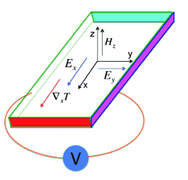
Figure 1: Schematic: geometry of the experiments considered in this paper.

Let us consider a conductor looped via a voltmeter in y-direction, placed in the magnetic field $\mathbf{H}$ oriented along z-axis, and subjected to the temperature gradient $\nabla_{x}T$  applied along x-axis (see Fig. 1). In a full generality, one can express the electric current density $\mathbf{j}$ components as:

$$\left(\begin{array}[]{c}j_{x}\\ j_{y}\end{array}\right)=\widehat{\sigma}\left(\begin{array}[]{c}E_{x}\\ E_{y}\end{array}\right)+\widehat{\beta}\left(\begin{array}[]{c}\nabla_{x}T\\ 0\end{array}\right),$$ (3)

where $\widehat{\sigma}$ and $\widehat{\beta}$ are conductivity and thermoelectric tensors, respectively. Further we restrict our consideration to the limit of magnetic fields weak by a parameter $\omega_{c}\tau\ll 1$, where $\omega_{c}$ is the cyclotron frequency, and $\tau$ is the elastic scattering time.

Dimensionality $d=3$ $d=2$ $d=1$ Fermi energy $\mu_{P}^{\left(d\right)}\left(0\right)$ (parabolic spectrum) $\mu_{P}^{\left(3\right)}\left(0\right)=\left(3\pi^{2}\right)^{2/3}\frac{\hbar^{2}}{2m}\left[n_{e}^{\left(3\right)}\right]^{2/3}$ $\mu_{P}^{\left(2\right)}\left(0\right)=\frac{\pi\hbar^{2}}{m}n_{e}^{\left(2\right)}$ $\mu_{P}^{\left(1\right)}\left(0\right)=\frac{2\pi^{2}\hbar^{2}}{m}\left[n_{e}^{\left(1\right)}\right]^{2}$ Chemical potential for degenerated FG (parabolic spectrum) $T\ll\mu_{P}^{\left(D\right)}\left(0\right)$ $\mu_{P}^{\left(3\right)}\left(T\right)=\mu_{P}^{\left(3\right)}\left(0\right)-\frac{\pi^{2}T^{2}}{6\mu_{P}^{\left(3\right)}\left(0\right)}$ $\mu_{P}^{\left(2\right)}\left(T\right)=\mu_{P}^{\left(2\right)}\left(0\right)$ $+T\ln\left[1-e^{-\frac{\mu_{P}^{\left(2\right)}\left(0\right)}{T}}\right]$ $\simeq\mu_{P}^{\left(2\right)}\left(0\right)-Te^{-\frac{\mu_{P}^{\left(2\right)}\left(0\right)}{T}}$ $\mu_{P}^{\left(1\right)}\left(T\right)=\mu_{P}^{\left(1\right)}\left(0\right)-\frac{\pi^{2}T^{2}}{12\mu_{P}^{\left(1\right)}\left(0\right)}$ Chemical potential for Boltzman FG (parabolic spectrum) $T\gg\mu_{P}^{\left(d\right)}\left(0\right)$ $\mu_{P}^{\left(3\right)}\left(T\right)=-\frac{3}{2}T\ln\frac{T}{\mu_{P}^{\left(3\right)}\left(0\right)}$ $\mu_{P}^{\left(2\right)}\left(T\right)=\mu_{P}^{\left(2\right)}\left(0\right)$ $+T\ln\left[1-e^{-\frac{\mu_{P}^{\left(2\right)}\left(0\right)}{T}}\right]$ $\simeq-T\ln\frac{T}{\mu_{P}^{\left(2\right)}\left(0\right)}$ $\mu_{P}^{\left(1\right)}\left(T\right)=-\frac{T}{2}\ln\frac{\pi^{4}T}{4\mu_{P}^{\left(1\right)}\left(0\right)}$ Fermi energy $\mu_{D}^{\left(d\right)}\left(0\right)$ (Dirac spectrum) $\mu_{D}^{\left(3\right)}\left(0\right)=\pi\hbar c\sqrt[3]{3n_{e}}$ $\mu_{D}^{\left(2\right)}\left(0\right)=\hbar c\sqrt{2\pi n_{e}}$ $\mu_{D}^{\left(1\right)}\left(0\right)=\pi\hbar cn_{e}$ Chemical potential for degenerated FG (Dirac spectrum) $T\ll\mu_{D}^{\left(d\right)}\left(0\right)$ $\mu_{D}^{\left(3\right)}\left(T\right)=\mu_{D}^{\left(3\right)}\left(0\right)-\frac{\pi^{2}T^{2}}{3\mu_{D}^{\left(3\right)}\left(0\right)}$ $\mu_{D}^{\left(2\right)}\left(T\right)=\mu_{D}^{\left(2\right)}\left(0\right)-\frac{\pi^{2}T^{2}}{12\mu_{D}^{\left(2\right)}\left(0\right)}$ $\mu_{D}^{\left(1\right)}\left(T\right)=T\ln\left[e^{\frac{\mu_{D}^{\left(1\right)}\left(0\right)}{T}}-1\right]$ $\simeq\mu_{D}^{\left(1\right)}\left(0\right)-Te^{-\frac{\mu_{D}^{\left(1\right)}\left(0\right)}{T}}$ Chemical potential for Boltzman FG (Dirac spectrum) $T\gg\mu_{D}^{\left(d\right)}\left(0\right)$ $\mu_{D}^{\left(3\right)}\left(T\right)=-3T\ln\frac{T}{\mu_{D}^{\left(3\right)}\left(0\right)}$ $\mu_{D}^{\left(2\right)}\left(T\right)=-2T\ln\frac{T}{\mu_{D}^{\left(2\right)}\left(0\right)}$ $\mu_{D}^{\left(1\right)}\left(T\right)=T\ln\left[e^{\frac{\mu_{D}^{\left(1\right)}\left(0\right)}{T}}-1\right]$ $\simeq-T\ln\left(\frac{T}{\mu_{D}^{\left(1\right)}\left(0\right)}\right)$

Table 1. The temperature dependencies of chemical potential in the systems of different dimensionalities, for carriers having a parabolic and linear dispersion, in the limits of Boltzmann and degenerate Fermi gases. Expressions related to the Boltzmann gas are shown on the grey background. $P$ and $D$ denote the expressions obtained for parabolic and Dirac dispersion cases, respectively.

For the heat flow$\ \mathbf{q}$ components one can write the similar equation:

$$\left(\begin{array}[]{c}q_{x}\\ q_{y}\end{array}\right)=\widehat{\gamma}\left(\begin{array}[]{c}E_{x}\\ E_{y}\end{array}\right)+\widehat{\zeta}\left(\begin{array}[]{c}\nabla_{x}T\\ 0\end{array}\right),$$ (4)

where the tensor $\widehat{\gamma}$ is related to $\widehat{\beta}$ by means of Onsager relation: $\widehat{\gamma}(H)=-T\widehat{\beta}(-H)$. Tensor $\widehat{\zeta}=-\frac{\pi^{2}T}{3e^{2}}\widehat{\sigma}$ mainly determines the value of thermal conductivity $\widehat{\kappa}$ Abrikosov . In the following we shall find the tensor $\widehat{\beta}$ and express the most important coefficients of the TM and TE transport through its components and conductivity tensor $\widehat{\sigma}$.

We limit ourselves to consideration of the case where the electric circuits are broken in both x,y-directions, so that $j_{x}=0$ (see Fig. 1):

$$j_{x}=\sigma_{xx}E_{x}+\sigma_{xy}E_{y}+\beta_{xx}\nabla_{x}T=0$$ (5)

$$j_{y}=\sigma_{yx}E_{x}+\sigma_{yy}E_{y}+\beta_{yx}\nabla_{x}T=0$$ (6)

The off-diagonal components of the TE tensor differ from zero only due to non-zero magnetic field applied. They can be determined from the fourth Maxwell equation Obraztsov ; VarlamovPRL and expressed in terms of the temperature derivative of the magnetization $M_{z}$:

$$\beta_{xy}=-\beta_{yx}=c\frac{\partial M_{z}}{\partial T},$$

where the latter can be expressed as the derivative of the thermodynamic potential $\Omega$ over magnetic field

$$M_{z}=-\frac{\partial\Omega}{\partial H_{z}}.$$

The electric field along x-direction induced by the temperature gradient can be determined using the condition of constancy of the electrochemical potential Eq. (2):

$$\nabla\left[e\varphi+\mu(T(x),n(x))\right]=0$$ (7)

and can be expressed in terms of the full derivative of the chemical potential:

$$E_{x}=-\nabla\varphi=\frac{1}{e}\left(\frac{d\mu}{dT}\right)\nabla_{x}T.$$ (8)

Here we have assumed that the electro-neutrality of our system is preserved (except for its surfaces, may be), and no volume charge is formed, so that $\nabla_{x}n=0.$ Substituting Eq. (8) to the first of the set of Eqs. (3) one finds that

$$\widehat{\beta}=\left(\begin{array}[]{cc}-\frac{\sigma_{xx}}{e}\left(\frac{d\mu}{dT}\right)&c\left(\frac{dM_{z}}{dT}\right)\\ -c\left(\frac{dM_{z}}{dT}\right)&-\frac{\sigma_{yy}}{e}\left(\frac{d\mu}{dT}\right)\end{array}\right).$$ (9)

Now we can proceed with obtaining TE and TM coefficients explicitly.

Seebeck tensor (differential thermoelectric power) $\widehat{Q}$ is related to the tensors $\widehat{\beta}$ and $\widehat{\sigma}:$

$$\widehat{Q}\left(H\right)=-\widehat{\sigma}^{-1}\left(H\right)\widehat{\beta}\left(H\right)=\frac{1}{e}\left(\frac{d\mu}{dT}\right)\widehat{I}-c\widehat{\sigma}^{-1}\widehat{e}\left(\frac{d\mathbf{M}}{dT}\right).$$ (10)

where $\widehat{e}=\left[\begin{array}[]{cc}0&1\\ -1&0\end{array}\right]$  is the Levi-Civitte tensor,$\widehat{I}$ is the identity tensor.

The chemical potential derivative can be found explicitly as:

$$\frac{d\mu}{dT}=\frac{\partial\mu}{\partial T}+\frac{\partial\mu}{\partial n}\frac{dn}{dT}.$$ (11)

For the reference case of an isotropic 3D metal with the parabolic spectrum in zero magnetic field

$$\frac{\partial\mu}{\partial n}=\frac{\hbar^{2}}{m}\frac{\pi^{4/3}}{\left(3n\right)^{1/3}}$$ (12)

and $dn/dT=\nu\partial\mu/\partial T$ with $\nu=mp_{F}/(\pi^{2}\hbar^{3})$ as density of states. Using these expressions one finds

$$\frac{d\mu}{dT}=2\frac{\partial\mu}{\partial T}.$$

The temperature derivative of a chemical potential for a degenerate electron gas is well-known (see, for example, Abrikosov ):

$$\mu(T)=\mu(0)-\frac{\pi^{2}T^{2}}{6}\frac{\nu^{\prime}\left(\mu\right)}{\nu\left(\mu\right)}.$$ (13)

As in the 3D case $\nu\left(\mu\right)\sim\sqrt{\mu\text{, }}$ thus $\partial\mu/\partial T=-\pi^{2}T/(6\mu),$ and consequently $d\mu/$ $dT=-\pi^{2}T/\left(3\mu\right).$This is why we obtain:

$$Q(T,0)=\frac{1}{e}\left(\frac{d\mu}{dT}\right)=-\frac{\pi^{2}T}{3e\mu}.$$

This expression exactly coincides with the Mott formula for a differential thermoelectric power Abrikosov , that demonstrates the equivalence of our approach to the classic result obtained the kinetic approach for a 3D metal.

Thomson coefficient, which describes alternatively heating or cooling of a current carrying conductor, can be also easily expressed now in terms of $\mu$ and $M$ temperature derivatives following the Thomson relation

$$\widehat{\mathcal{T}}=T\frac{d\widehat{Q}}{dT}=\frac{T}{e}\left(\frac{d^{2}\mu}{dT^{2}}\right)\widehat{I}-cT\widehat{\sigma}^{-1}\widehat{e}\left(\frac{d^{2}\mathbf{M}}{dT^{2}}\right).$$ (14)

In the absence of magnetic field

$$\widehat{\mathcal{T}}(T,H=0)=\frac{T}{e}\left(\frac{d^{2}\mu}{dT^{2}}\right)\widehat{I}.$$ (15)

Using the expressions for the chemical potential summarized in the Table 1 one can see that the Thomson coefficient behaves quite differently for Dirac and normal carriers. For example, in the degenerate 2D gas of carriers with a parabolic dispersion the Thomson coefficient is

$$\mathcal{T}_{(P)}^{\left(2\right)}=\frac{\left[\mu_{(P)}^{\left(2\right)}\left(0\right)\right]^{2}}{eT^{2}}\exp\left(-\frac{\mu_{(P)}^{\left(2\right)}\left(0\right)}{T}\right),$$ (16)

while for 2D Dirac carriers it differs not only by its temperature dependence but also in its sign:

$$\mathcal{T}_{(D)}^{\left(2\right)}=-\frac{\pi^{2}T}{6e\mu_{D}^{\left(2\right)}\left(0\right)}.$$ (17)

One can see that in a wide range of temperatures up to $T\lesssim 0.2\mu_{P}^{\left(2\right)}\left(0\right)$ Thomson coefficient for the normal carriers is exponentially small. In the same time for Dirac fermions the Thomson coefficient is of the opposite sign and growth in its absolute value linearly with temperature. Moreover, at high temperatures the behavior of the Thomson coefficient is non-monotonous for normal carriers, while for the Dirac spectrum it is a monotonous saturating function (see Fig. 2).

Nernst-Ettingshausen effect is the thermal analog of the Hall effect and it consists in the appearance of an electric field $E_{y}$ perpendicular to the mutually perpendicular magnetic field $H(\parallel z)$ and temperature gradient $(\nabla_{x}T)$ (see Fig. 1). It is characterized by the Nernst coefficient

$$\nu=\frac{E_{y}}{(-\nabla_{x}T)H},$$ (18)

which can be expressed in terms of the resistivity and thermoelectric tensors Anselm :

$$\nu=-\left(\rho_{xx}\beta_{xy}+\rho_{xy}\beta_{yy}\right)/H.$$ (19)

Substituting in Eq. (19) the expressions for the thermoelectric tensor components obtained above, we arrive at:

$$\nu=\frac{\sigma_{xx}}{e^{2}nc}\left(\frac{d\mu}{dT}\right)+\frac{c\rho_{yy}}{H}\left(\frac{dM_{z}}{dT}\right).$$ (20)

The first term here is governed by the temperature dependence of the chemical potential, while the second is related to magnetization currents. In our reference case of a 3D metal the second term is negligible by a parameter $\left(k_{F}l\right)^{-1}\ll 1$, with $k_{F}$ being the Fermi wave-vector, $l$ being the mean free path. Using Eq. (13) one easily reproduces the well-known Sondheimer formula 1948Sondheimer

$$\nu=\frac{\sigma_{xx}}{e^{2}nc}\left(\frac{d\mu}{dT}\right)=-\frac{\sigma_{xx}}{e^{2}nc}\frac{\pi^{2}T}{3\mu}=-\frac{\pi^{2}T}{3\mu}\frac{\tau}{mc}.$$ (21)

In fluctuating superconductors the role of the second term in Eq. (20) becomes crucial: it “saves” the third law of thermodynamics in the vicinity of the second critical field $H_{c2}(0)$ SSVG09 . The oscillations of Nernst-Ettingshausen coefficient in graphene obtained within the present approach VarlamovPRL demonstrate a remarkable agreement with experimental data Zuev .

In the rest of this Letter we summarize the useful expressions for other important TE and TM coefficients following the approach formulated here.

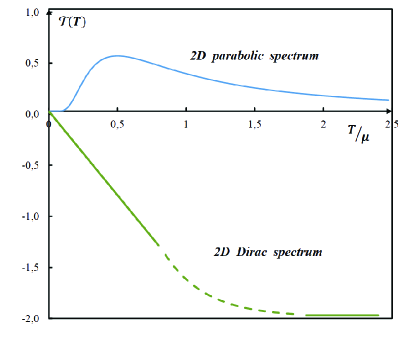
Figure 2: Schematic: Thomson coefficient vs temperature in the 2D case. The Thomson coefficient is positive and non-monotonous for carriers with a parabolic dispersion, while it is negative and saturates in the case of a Dirac spectrum.

Peltier tensor which describes the heat generation by electric current, is given by Kelvin relation (see e.g. Abrikosov ) and can also be expressed in terms of conductivity and thermoelectric tensors

$$\widehat{\Pi}\left(T,H\right)=T\widehat{Q}\left(T,H\right)=-T\widehat{\sigma}^{-1}\left(H\right)\widehat{\beta}\left(H\right).$$ (22)

At zero magnetic field, it has only diagonal components:

$$\Pi\left(T,0\right)=\frac{T}{e}\left(\frac{d\mu}{dT}\right).$$ (23)

Interestingly, while the whole system is out of thermal equilibrium in the presence of electric current, the Peltier coefficient can still be linked to the thermal derivative of the chemical potential!

The thermal conductivity tensor $\widehat{\kappa}$ describes the ability of a material subject to a temperature gradient to conduct heat. It can be expressed through the elements of TE tensor and electric conductivity

$$\widehat{\kappa}=-\frac{\pi^{2}T}{3e^{2}}\widehat{\sigma}\left(\widehat{I}-\frac{3e^{2}}{\pi^{2}}\left[\widehat{\beta}\widehat{\sigma}^{-1}\right]^{2}\right).$$ (24)

Righi-Leduc effect describes the heat flow resulting from a perpendicular temperature gradient in the absence of electric current. Righi-Leduc coefficient can be expressed through the diagonal elements of thermal conductivity and conductivity tensors as

$$L=\frac{\sigma_{xx}}{enc}\kappa_{yy}.$$ (25)

Finally, we would like to discuss limitations of our approach. We have largely used the electro-neutrality condition $\nabla_{x}n=0$, which may fail in certain semiconductor systems where the volume charge effects are important. For the same reason, this approach fails to account for electric currents induced by a phonon drag.

In conclusion, the crucial function which governs all TE and TM constants listed above is the temperature derivative of the chemical potential $\frac{d\mu}{dT}$. This simple observation opens way to the prediction of TE and TM effects in new structures and materials. In particular, it shows that TE and TM properties may be strongly different in systems with Dirac fermions and normal carriers.

The authors acknowledge helpful discussions with I. Chikina and S.G. Sharapov. This work has been supported by the EU IRSES program ”SIMTECH”.

References

- (1) N. F. Mott and H. Jones The Theory of the Properties of Metals and Alloys 1st edition (Oxford: Clarendon)(1936).
- (2) E. H. Sondheimer, Proc. R. Soc. London, Ser A, 193, 484 (1948).
- (3) Allen J. Bard and Larry R. Faulkner, Electrochemical Methods: Fundamentals and Applications, Wiley; 2nd edition (2000), Section 2.2.4(a),4-5.
- (4) N. W. Ashcroft and N. D. Mermin, Solid State Physics, Brooks-Cole (1976), page 593.
- (5) O. Madelung, Introduction to Solid-State: Theory, Springer, Berlin (1995), page 198.
- (6) A.A. Abrikosov Fundamentals of the Theory of Metals, Elsevier, Amsterdam (1989).
- (7) Yu. N. Obraztsov, Sov. Phys. Solid State, 6 331 (1964).
- (8) I. A. Luk’yanchuk, A.A. Varlamov and A.V. Kavokin, Phys. Rev. Lett. 107, 016601 (2011).
- (9) A.I. Anselm, Introduction to Semiconductor Theory, 2nd edition Prentice-Hall, Englewood Cliffs, N.J. (1982).
- (10) M. N. Serbyn, M. A. Skvortsov, A. A. Varlamov, and V. Galitski , Phys. Rev. Lett. 102, 067001 (2009).
- (11) A. A. Varlamov and A.V. Kavokin, Europhysics Letters, 86, 47007 (2009).
- (12) Y. M. Zuev, W. Chang and P. Kim, Phys. Rev. Lett. 102, 096807 (2009).