Observational Constraints on Modified Chaplygin Gas from Cosmic Growth

Abstract

We investigate the linear growth function for the large scale structures of the universe considering modified Chaplygin gas as dark energy. Taking into account observational growth data for a given range of redshift from the Wiggle-Z measurements and rms mass fluctuations from Ly-$\alpha$ measurements we numerically analyze cosmological models to constrain the parameters of the MCG. The observational data of Hubble parameter with redshift ($Z$) is also considered. The Wang-Steinhardt ansatz for growth index $\gamma$ and growth function $f$ (defined as $f=\Omega_{m}^{\gamma}(a)$) are considered for the numerical analysis. The best-fit values of the equation of state parameters obtained here is employed to study the growth function $(f)$, growth index ($\gamma$) and state parameter ($\omega$) with redshift $z$. We note that MCG satisfactorily accommodates an accelerating phase followed by a matter dominated universe.

1 Introduction

Recent cosmological observations from supernova [1, 2, 3, 4, 5], WMAP [6, 7, 8, 9, 10], BAO oscillation data [11] predicted that the present universe is passing through a phase of accelerating expansion which might have fuelled due to existence of a new source called dark energy. In cosmological observations the expansion rate $H(z)$ is related to various redshift which are employed to obtain different parameters e.g., distance modulus parameter is one of them. Although the analysis provide us with a satisfactory understanding of cosmological dynamics it does not give a complete understanding of the evolution of the universe. Consequently additional observational inputs namely, cosmic growth of the inhomogeneous part of the universe for its structure formation are considered. The growth of the large scale structures derived from linear matter density contrast $\delta(z)\equiv\frac{\delta\rho_{m}}{\rho_{m}}$ of the universe is considered an important tool in constraining cosmological model parameters. To describe the evolution of the inhomogeneous energy density it is preferable to parametrize the growth function $f=\frac{d\log\delta}{d\log a}$ in terms of growth index ($\gamma$). Initially Peebles [12] and subsequently Wang and Steinhardt [13] parametrized $\delta$ in terms of $\gamma$ to obtain cosmologies which are useful in different contexts discussed in the literature [14, 15, 16, 17, 18, 19, 20, 21, 22, 23]. It is possible to understand dark energy in cosmology from the analysis of observational data from the observed expansion rate ($H(z)$) and growth of matter density contrast $\delta(z)$ data simultaneously.

It is known that in general theory of relativity ordinary matter fields available from standard model of particle physics fails to account the present observations. As a result modification of the matter sector of the Einstein-Hilbert action with exotic matter is considered in the literature. Chaplygin gas (CG) is considered to be one such candidate for dark energy. The equation of state (henceforth, EoS) for CG is

$$p=-\frac{A}{\rho}$$ (1.1)

where $A$ is positive constant. It may be important to mention here that the initial idea of CG originated in Aerodynamics [24]. But it is ruled out in cosmology from observations. Subsequently the equation of state for CG is generalized to incorporate different aspects of the observational universe. The equation of state for generalized Chaplygin gas (in short, GCG) [25, 26] is given by

$$p=-\frac{A}{\rho^{\alpha}}$$ (1.2)

with $0\leq\alpha\leq 1$. In the above EoS, Chaplygin gas corresponds to $\alpha=1$ [24]. It has two free parameters $A$ and $\alpha$. Initially GCG behaves like a pressureless fluid at the early stages of the evolution of the universe, but at a later stage it behaves like a cosmological constant. In the context of string theory Chaplygin gas emerges from the dynamics of a generalized d-brane in a (d+1,1) space time. It can be described by a complex scalar field which is obtained from a generalized Born-Infeld action. More recently modified Chaplygin gas (in short, MCG) is considered in describing dark energy because of its negative pressure [27, 28, 29]. The equation of state for the MCG is given by:

$$p=B\rho-\frac{A}{\rho^{\alpha}}$$ (1.3)

where $A$, $B$, $\alpha$ are positive constants with $0\leq\alpha\leq 1$ . The above EoS reduces to that of GCG model [25, 26] when one sets $B=0$. A cosmological constant $\Lambda$ emerged by setting $\alpha=-1$ and $A=1+B$. If one considers $A=0$, it reduces to an EoS which describes a perfect fluid with $\omega=B$, e.g., a quintessence model [30]. MCG contains one more free parameter namely, $B$ over GCG..It may be pointed out here that MCG is a single fluid model which unify dark matter and dark energy. MCG behaves as dark matter when its energy density evolves as $\rho\propto a^{-3}$ (where $a(t)$ represents the scale factor) in the early epoch whereas the constant energy density behaves as dark energy accommodating late time acceleration [31]. The MCG is consistent with (i) Gravitational lensing test [32, 33] and (ii) Gamma-ray bursts [34].

In this paper we determine constraints on EoS parameters of the MCG using different observational data namely, the growth function and growth index in a FRW universe. The growth data and the Stern data set [35] of $H(z)$ vs. $z$ are considered here for the analysis. The growth data given in Table -1 consists of a number of data points within redshift range (0.15 to 3.8) which are related to growth function $f$. It may be pointed out here that redshift that estimates the linear growth rate are considered from various projects/surveys including the latest Wiggle-Z measurements. Gupta et al. [36] obtained constrains on GCG parameters using the above data. Cosmological model dominated by viscous dark fluid is also considered in Ref.[37] where it is found that viscous fluid mimics as $\Lambda$CDM model when coefficient of viscosity varies as $\rho^{-1/2}$ providing excellent agreement both with supernova and $H-z$ data. The viscous cosmological model is found analogous to GCG model. In addition to the above data other observational set of growth data given in (Table- 2 from various sources such as: the redshift distortion of galaxy power spectra [38], root mean square $(rms)$ mass fluctuation ($\sigma_{8}(z)$) obtained from galaxy and Ly-$\alpha$ surveys at various redshifts [39, 40], weak lensing statistics [41], baryon acoustic oscillations [11], X-ray luminous galaxy clusters [42], Integrated Sachs-Wolfs (ISW) Effect [43, 44, 45, 46, 47] etc. are important. It is known that redshift distortions are caused by velocity flow induced by gravitational potential gradient which evolved due to the growth of the universe under gravitational attraction and dilution of the potentials due to the cosmic expansion. The gravitational growth index $\gamma$ has considerable impact on the redshift distortion [14]. The cluster abundance evolution, however, found strongly depends on rms mass fluctuations ($\sigma_{8}(z)$) [13].

We adopt here chi-square minimization technique to constrain different parameters of the EoS for a viable cosmological model considering MCG. In the analysis total chi-square is constituted using the growth data and the $(H(z)-z)$ OHD data. The best-fit values of the model parameters are then determined from the chi-square function to study evolution of the universe. The paper is organized as follows : In sec.2, we set up Einstein field equations. In sec.3, growth index parametrization in terms of EoS parameters is given. In sec.4, constraint on the EoS parameters obtained from observational data are presented. Finally, we conclude in sec.5.

2 Einstein Field Equations

The Einstein field equation is given by

$$R_{\mu\nu}-\frac{1}{2}g_{\mu\nu}R=8\pi G\;T_{\mu\nu}$$ (2.1)

where $R_{\mu\nu}$ represents Ricci tensor, $R$ represents Ricci scalar, $T_{\mu\nu}$ represents energy momentum tensor and $g_{\mu\nu}$ represents the metric tensor in 4-dimensions. We consider a Robertson-Walker metric which is given by

$$ds^{2}=-dt^{2}+a^{2}(t)\left[\frac{dr^{2}}{1-kr^{2}}+r^{2}(d\theta^{2}+sin^{2}\theta\;d\phi^{2})\right]$$ (2.2)

where $k=0,+1(-1)$ is the curvature parameter in the spatial section representing flat, closed (open) universe and $a(t)$ is the scale factor of the universe with $r,\theta,\phi$ co-moving co-ordinates.

Using metric (2.2) in the Einstein field eq. (2.1), we obtain the following equations:

$$3\left(\frac{\dot{a}^{2}}{a^{2}}+\frac{k}{a^{2}}\right)=8\pi G\;\rho,$$ (2.3)

$$2\frac{\ddot{a}}{a}+\frac{\dot{a}^{2}}{a^{2}}+\frac{k}{a^{2}}=-8\pi G\;p,$$ (2.4)

where $\rho$ and $p$ represent the energy density and pressure respectively. The conservation equation is given by

$$\frac{d\rho}{dt}+3H\left(\rho+p\right)=0,$$ (2.5)

where $H=\frac{\dot{a}}{a}$ is Hubble parameter.

Using EoS given by eq.(1.3) in eq.(2.5),and integrating once one obtains energy density for a modified Chaplygin gas which is given by

$$\rho_{mcg}=\rho_{0}\left[A_{S}+\frac{1-A_{S}}{a^{3(1+B)(1+\alpha)}}\right]^{\frac{1}{1+\alpha}}$$ (2.6)

where $A_{S}=\frac{A}{1+B}\frac{1}{\rho_{0}^{\alpha+1}}$ with $B\neq-1$, $\rho_{o}$ is an integration constant. The scale factor of the universe is related to the redshift parameter ($z$) as $\frac{a}{a_{0}}=\frac{1}{1+z}$, where we choose the present scale factor of the universe $a_{0}=1$ for convenience. The MCG model parameters are $A_{S}$, $B$ and $\alpha$. From eq. (2.6), it is evident that the positivity condition of the energy density is ensured when $0\leq A_{S}\leq 1$. From eq. (2.6), one recovers the standard $\Lambda CDM$ model for $\alpha=0$ and $B=0$. The Hubble parameter can be expressed as a function of redshift using the field eq. (2.3), which is given by

$$H(z)=H_{0}[\Omega_{b0}(1+z)^{3}+$$

$$\;\;\;\;\;(1-\Omega_{b0})[(A_{s}+(1-A_{s})(1+z)^{3(1+B)(1+\alpha)})^{\frac{1}{1+\alpha}}]]^{\frac{1}{2}}.$$ (2.7)

where $\Omega_{b0}$, $H_{0}$ represent the present baryon density and present Hubble parameter respectively.

The sound speed is given by

$$c^{2}_{s}=\frac{\delta p}{\delta\rho}=\frac{\dot{p}}{\dot{\rho}}$$ (2.8)

which reduces to

$$c^{2}_{s}=B+\frac{A_{s}\alpha(1+B)}{\left[A_{s}+(1-A_{s})(1+z)^{3(1+B)(1+\alpha)})\right]}.$$ (2.9)

In terms of state parameter it becomes

$$c^{2}_{s}=-\alpha\omega+B(1+\alpha).$$ (2.10)

It may be mentioned here that for causality and stablity under perturbation it is required to satisfy the inequality condition $c_{s}^{2}\leq 1$ [30].

3 Parametrization of the Growth Index

The growth rate of the large scale structures is derived from matter density perturbation $\delta=\frac{\delta\rho_{m}}{\rho_{m}}$ (where $\delta\rho_{m}$ represents the fluctuation of matter density $\rho_{m}$) in the linear regime which satisfies

$$\ddot{\delta}+2\frac{\dot{a}}{a}\dot{\delta}-4\pi G_{eff}\rho_{m}\delta=0.$$ (3.1)

The field equation for the background cosmology comprising both matter and MCG in FRW universe are given below

$$\left(\frac{\dot{a}}{a}\right)^{2}=\frac{8\pi G}{3}(\rho_{b}+\rho_{mcg}),$$ (3.2)

$$2\frac{\ddot{a}}{a}+\left(\frac{\dot{a}}{a}\right)^{2}=-8\pi G\omega_{mcg}\rho_{mcg}$$ (3.3)

where $\rho_{b}$ represents the background energy density and $\omega_{mcg}$ represents the state parameter for MCG which is given by

$$\omega_{mcg}=B-\frac{A_{s}(1+B)}{\left[A_{s}+(1-A_{s})(1+z)^{3(1+B)(1+\alpha)})\right]}.$$ (3.4)

We now replace the time ($t$) variable to $ln\,a$ in eq.(3.1) and obtain

$$(\ln\delta)^{{}^{\prime\prime}}+(\ln\delta)^{{}^{\prime}2}+(\ln\delta)^{{}^{\prime}}\left[\frac{1}{2}-\frac{3}{2}\omega_{mcg}(1-\Omega_{m}(a))\right]=\frac{3}{2}\Omega_{m}(a)$$ (3.5)

where

$$\Omega_{m}(a)=\frac{\rho_{m}}{\rho_{m}+\rho_{mcg}}.$$ (3.6)

The effective matter density is given by $\Omega_{m}=\Omega_{b}+(1-\Omega_{b})(1-A_{s})^{(1/1+\alpha)}$ [48]. Using the energy conservation eq. (2.5) and changing the variable from $\ln a$ to $\Omega_{m}(a)$ once again, the eq. (3.5) can be expressed in terms of the logarithmic growth factor $f=\frac{d\log\delta}{d\log a}$ which is given by

$$3\omega_{mcg}\Omega_{m}(1-\Omega_{m})\frac{df}{d\Omega_{m}}+f^{2}+f\left[\frac{1}{2}-\frac{3}{2}\omega_{mcg}(1-\Omega_{m}(a))\right]=\frac{3}{2}\Omega_{m}(a).$$ (3.7)

The logarithmic growth factor $f$, according to Wang and Steinhardt [13] is given by

$$f=\Omega_{m}^{\gamma}(a)$$ (3.8)

where $\gamma$ is the growth index parameter. In the case of flat dark energy model with constant state parameter $\omega_{0}$, the growth index $\gamma$ is given by

$$\gamma=\frac{3(\omega_{0}-1)}{6\omega_{0}-5}.$$ (3.9)

For a $\Lambda CDM$ model, it reduces to $\frac{6}{11}$ [14, 49], for a matter dominated model, one gets $\gamma=\frac{4}{7}$ [50, 51]. One can also write $\gamma$ as a parametrized function of redshift parameter $z$. One such parametrisation is $\gamma(z)=\gamma(0)+\gamma^{{}^{\prime}}z$, with $\gamma^{{}^{\prime}}\equiv\frac{d\gamma}{dz}|_{(z=0})$ [52, 53]. It has been shown recently [54] that the parametrization smoothly interpolates a low and intermediate redshift range to a high redshift range up to the cosmic microwave background scale. The above parametrization is also taken up in different contexts [55]. In this paper we parametrize $\gamma$ in terms of MCG parameters namely, $A_{s}$, $\alpha$ and $B$. Therefore, we begin with the following ansatz which is given by

$$f=\Omega_{m}^{\gamma(\Omega_{m})}(a)$$ (3.10)

where the growth index parameter $\gamma(\Omega_{m})$ can be expanded in Taylor series around $\Omega_{m}=1$ as

$$f=\gamma(\Omega_{m})\hskip 227.62204pt$$

$$\;\;\;\;\;\;\;\;=\gamma(\Omega_{m}-1)+(\Omega_{m}-1)\frac{d\gamma}{d\Omega_{m}}(\Omega_{m}=1)+O(\Omega_{m}-1)^{2}.$$ (3.11)

Consequently eq.(3.11) can be rewritten in terms of $\gamma$ as

$$3\omega_{mcg}\Omega_{m}(1-\Omega_{m})\ln\Omega_{m}\frac{d\gamma}{d\Omega_{m}}-3\omega_{mcg}\Omega_{m}(\gamma-\frac{1}{2})+$$

$$\;\;\;\;\;\Omega_{m}^{\gamma}-\frac{3}{2}\Omega_{m}^{1-\gamma}+3\omega_{mcg}\gamma-\frac{3}{2}\omega_{mcg}+\frac{1}{2}=0.$$ (3.12)

Differentiating once again the above equation around $\Omega_{m}=1$, one obtains zeroth order term in the expansion for $\gamma$ which is given by

$$\gamma=\frac{3(1-\omega_{mcg})}{5-6\omega_{mcg}},$$ (3.13)

it agrees with dark energy model for a constant $\omega_{0}$ (eq. 3.9). In the same way differentiating it twice and thereafter by a Taylor expansion around $\Omega_{m}=1$, one obtains the first order terms in the expansion which is given by

$$\frac{d\gamma}{d\Omega_{m}}|_{\Omega_{m}=1}=\frac{3(1-\omega_{mcg})(1-\frac{3\omega_{mcg}}{2})}{125(1-\frac{6\omega_{mcg}}{5})^{3}}.$$ (3.14)

Substituting it in eq. (3.11), $\gamma$ is obtained, the first order term in this case is approximated to

$$\gamma=\frac{3(1-\omega_{mcg})}{5-6\omega_{mcg}}+(1-\Omega_{m})\frac{3(1-\omega_{mcg})(1-\frac{3\omega_{mcg}}{2})}{125(1-\frac{6\omega_{mcg}}{5})^{3}}.$$ (3.15)

Using the expression of $\omega_{mcg}$ in the above, $\gamma$ can be parametrised with MCG parameters. We define normalised growth function $g$ from the numerically obtained solution using eq. (3.5) which is given by

$$g(z)\equiv\frac{\delta(z)}{\delta(0)}.$$ (3.16)

The corresponding normalised growth function obtained from the parametrized form of $f$ follows from eq.(3.10) which is given by

$$g_{th}(z)=\exp\oint\Omega_{m}(a)^{\gamma}\frac{da}{a}.$$ (3.17)

The above expression will be employed to construct chi-square function in the next section.

4 Observational Analysis

z	$f_{obs}$	$\sigma$	$Ref.$
$0.15$	0.51	0.11	[56, 57]
$0.22$	0.60	0.10	[58]
$0.32$	0.654	0.18	[59]
$0.35$	0.70	0.18	[60]
$0.41$	0.70	0.07	[58]
$0.55$	0.75	0.18	[61]
$0.60$	0.73	0.07	[58]
$0.77$	0.91	0.36	[62]
$0.78$	0.70	0.08	[58]
$1.4$	0.90	0.24	[63]
$3.0$	1.46	0.29	[64]

Table 1: Data for the observed growth functions $f_{obs}$ used in our analysis

z	$\sigma_{8}$	$\sigma_{\sigma{{}_{8}}}$	$Ref$
$2.125$	0.95	0.17	[39]
$2.72$	0.92	0.17
$2.2$	0.92	0.16	[40]
$2.4$	0.89	0.11
$2.6$	0.98	0.13
$2.8$	1.02	0.09
$3.0$	0.94	0.08
$3.2$	0.88	0.09
$3.4$	0.87	0.12
$3.6$	0.95	0.16
$3.8$	0.90	0.17
$0.35$	0.55	0.10	[65]
$0.6$	0.62	0.12
$0.8$	0.71	0.11
$1.0$	0.69	0.14
$1.2$	0.75	0.14
$1.65$	0.92	0.20

Table 2: Data for the rms mass fluctuations ($\sigma_{8}$) at various redshift

The redshift distortion parameter $\beta$, is related to the growth function $f$ as $\beta=\frac{f}{b}$, where $b$ represents the bias factor connecting total matter perturbation ($\delta$) and galaxy perturbations ( $\delta_{g}$ ) ($b=\frac{\delta_{g}}{\delta}$) [58, 60, 61, 63]. The data for $\beta$ and $b$ at various redshifts are taken from Ref. [58, 66]. In the present case we analyze cosmological models in the presence of modified Chaplygin gas in respect of cosmic growth function. As it is not possible to determine $\beta$ as is pointed out in Ref. [64], we use other power spectrum amplitudes of Ly-$\alpha$ forest data.

z Data	$H(z)$	$\sigma$
0.00	73	$\pm$ 8.0
0.10	69	$\pm$ 12.0
0.17	83	$\pm$ 8.0
0.27	77	$\pm$ 14.0
0.40	95	$\pm$ 17.4
0.48	90	$\pm$ 60.0
0.88	97	$\pm$ 40.4
0.90	117	$\pm$ 23.0
1.30	168	$\pm$ 17.4
1.43	177	$\pm$ 18.2
1.53	140	$\pm$ 14.0
1.75	202	$\pm$ 40.4

Table 3: $H(z)vs.z$ data from Stern et al. [35]

We define chi-square of the growth function $f$ as

$$\chi^{2}_{f}(A_{s},B,\alpha)=\Sigma\left[\frac{f_{obs}(z_{i})-f_{th}(z_{i},\gamma)}{\sigma_{f_{obs}}}\right]^{2}$$ (4.1)

where $f_{obs}$ and $\sigma_{f_{obs}}$ are obtained from Table-1. However, $f_{th}(z_{i},\gamma)$ is obtained from eqs. (3.10) and (3.15). Another observational probe for the matter density perturbation $\delta(z)$ is derived from the redshift dependence of the rms mass fluctuation $\sigma_{8}(z)$. The $rms$ mass fluctuation $\sigma_{8}(z)$ is defined as

$$\sigma^{2}(R,z)=\int_{0}^{\inf}W^{2}(kR)\Delta^{2}(k,z)dk/k$$ (4.2)

where

$$W(kR)=3\left(\frac{\sin(kR)}{(kR)^{3}}-\frac{\cos(kR)}{(kR)^{2}}\right)r,$$ (4.3)

$$\Delta^{2}(kz)=4\pi k^{3}P_{\delta}(k,z),$$ (4.4)

with $R=8h^{-1}$ Mpc. In the above $P_{\delta}(k,z)\equiv(\delta^{2}_{k})$ represents the mass power spectrum at redshift ($z$). The function $\sigma_{8}(z)$ is related to $\delta(z)$ as

$$\sigma_{8}(z)=\frac{\delta(z)}{\delta(0)}\sigma_{8}|_{(z=0)}$$ (4.5)

which implies

$$s_{th}(z_{1},z_{2})\equiv\frac{\sigma_{8}(z_{1})}{\sigma_{8}(z_{2})}=\frac{\delta(z_{1})}{\delta(z_{2})}=\frac{\exp\left[\int_{1}^{\frac{1}{1+z_{1}}}\Omega_{m}(a)^{\gamma}\frac{da}{a}\right]}{\exp\left[\int_{1}^{\frac{1}{1+z_{2}}}\Omega_{m}(a)^{\gamma}\frac{da}{a}\right]}.$$ (4.6)

Currently available data points $\sigma_{8}(z_{i})$ are taken from the observed redshift evolution of the flux power spectrum of Ly-$\alpha$ forest [39, 40, 65]. Using these we define a new chi-square function which is given by

$$\chi^{2}_{s}(A_{s},B,\alpha)=\Sigma\left[\frac{s_{obs}(z_{i},z_{i+1})-s_{th}(z_{i},z_{i+1})}{\sigma_{s_{obs,i}}}\right]^{2}.$$ (4.7)

For the numerical analysis we use data given in Table- 2 . From the Hubble parameter vs. redshift data [35] we define another chi-square $\chi^{2}_{H-z}$ function which is given by

$$\chi^{2}_{H-z}(H_{0},A_{s},B,\alpha,z)=\sum\frac{(H(H_{0},A_{s},B,\alpha,z)-H_{obs}(z))^{2}}{\sigma^{2}_{z}}$$ (4.8)

where $H_{obs}(z)$ is the observed Hubble parameter at redshift $z$ and $\sigma_{z}$ is the error associated with that particular observation as shown in Table -3. Now considering all the observations mentioned above, we consider total chi-square function which is given by

$$\chi^{2}_{total}(A_{s},B,\alpha)=\chi^{2}_{f}(A_{s},B,\alpha)+\chi^{2}_{s}(A_{s},B,\alpha)+\chi^{2}_{H-z}(A_{s},B,\alpha).$$ (4.9)

In this case the best fit value is obtained minimizing the chi-square function. Finally we draw contours at different confidence limits to determine limiting range of values of the EoS parameters for the MCG. We now minimize the chi-square $\chi^{2}_{f}(A_{s},B,\alpha)$ function with the growth rate data set.

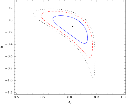
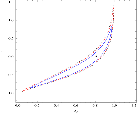
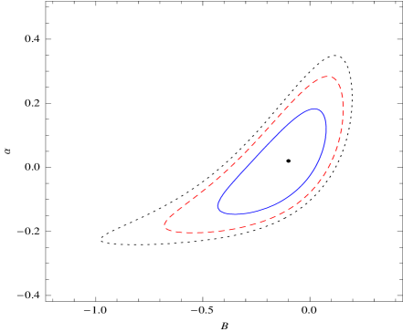
Figure 1: Contours from growth data at $68.3\%$(Solid) $90.0\%$ (Dashed) and $95.4\%$ (Dotted) confidence limit at best-fit values $A_{s}$=0.81,$B=-0.10$,$\alpha$=0.02.

The best-fit values of the EoS parameters are determined from minimization of chi-squares constituted from growth function (f), growth +rms mass fluctuation, growth +rms mass fluctuation+ OHD separately which are shown in Table-4. It appears from the analysis that the $A_{s}$ and $\alpha$ values are least from Growth+rms mass fluctuation+OHD but the parameters are positive. However, the best fit value of $B$ in the later case is a small positive number although a negative value for $B$ is permitted by other two observations.

Using the best fit values for growth data, rowth+ rms mass fluctuation data and rowth+ rms mass fluctuation data+OHD from Table-4 we draw contours for (i) $B$ vs. $A_{s}$ in figs. 1(a), 2(a) and 3(a) (ii) $\alpha$ vs. $A_{s}$ in figs. 1(b), 2(b) and 3(b) and (iii) $\alpha$ vs. $B$ in figs. 1(c), 2(c) and 3(c) respectively. Allowed range of values of the EoS parameters are then determined from the contours. In Table-5 we present allowed range of values of $A_{s}$ and $B$ (with 95.4 % confidence limit) for the three cases. It is observed that the range of values for $A_{s}$ and $B$ are tight. We note that both positive and negative values of $B$ parameters are possible. In Table-6 the range of values of $A_{s}$ and $\alpha$ are shown. It is evident from Growth+ rms mass fluctuation data+OHD analysis, that the lower bound on $A_{s}$ is decreased with a tight constraint but both positive and negative values of $\alpha$ are permissible. In Table-7 the range of values of $B$ and $\alpha$ are shown. It is evident from Growth+ rms mass fluctuation data+OHD analysis that the range of both $B$ and $\alpha$ are small. Both positive and negative values of the parameters are admitted.

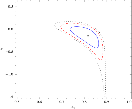
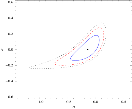
Figure 2: Contours from growth+rms mass fluctuations ($\sigma_{8}$) data at $68.3$%(Solid) $90.0\%$ (Dashed) and $95.4\%$ (Dotted) confidence limit at best-fit values :$A_{s}$=0.816,$B$=-0.146,$\alpha$=0.004

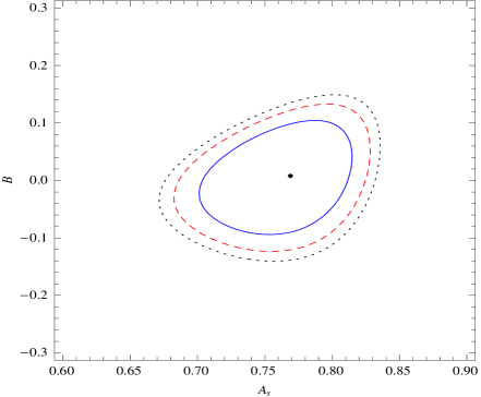
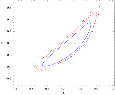
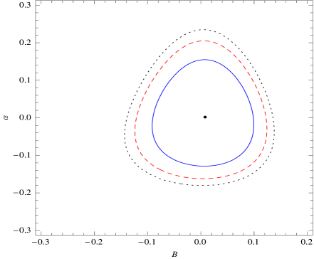
Figure 3: Contours from growth+rms mass fluctuations ($\sigma_{8}$)+OHD data at $68.3\%$(Solid) $90.0\%$ (Dashed) and $95.4\%$ (Dotted) confidence limit at best-fit values:$A_{s}$=0.769,$B$=0.008,$\alpha$=0.002

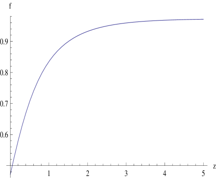
Figure 4: Evolution of growth function f with redshift at best-fit values :$A_{s}$=0.769,$B$=0.008,$\alpha$=0.002.

In fig. (4) the growth function $f$ is plotted with redshift $z$ using best fit values of model parameters. It is evident that the growth function $f$ lies in the range 0.472 to 1.0 for redshift between $z=0$ to $z=5$. Initially $f$ remains a constant but it falls sharply at low redshifts, indicating the fact that major growth of our universe have occurred at the early epoch with moderate redshift value.

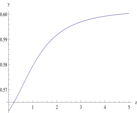
Figure 5: Evolution of growth index $\gamma$ with redshift at best-fit values :$A_{s}$=0.769,$B$=0.008,$\alpha$=0.002.

In fig. (5) we plot the variation of the growth index ( $\gamma$ ) with redshift ($z$). It is evident that the growth index ( $\gamma$) varies between 0.562 to 0.60 for a variation of redshift between $z=0$ to $z=5$. Thus we observe a sharp fall in the values of $\gamma$ at low redshift.

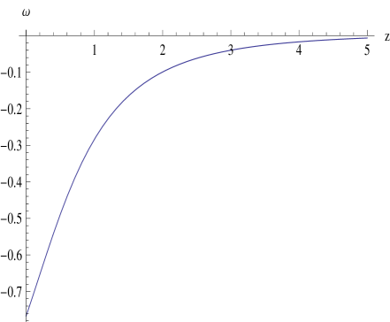
Figure 6: Evolution of the state parameter ($\omega$) at best-fit values:$A_{s}$=0.769,$B$=0.008,$\alpha$=0.002

In fig. (6) the variation of the state parameter ($\omega$) is plotted with $z$. It is found that the state parameter ($\omega$) varies from -0.767 at the present epoch ($z=0$) to $\omega\rightarrow 0$ at intermediate redshift ($z=5$). This result indicates that the universe is now passing through an accelerating phase which is dominated by dark energy whereas in the early universe ($z>5$) it was dominated by matter permitting a decelerating phase.

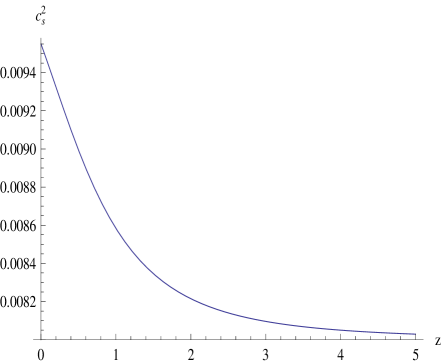
Figure 7: Sound speed variations with redshift at best-fit values :$A_{s}$=0.769,$B$=0.008,$\alpha$=0.002

The variation of sound speed $c_{s}^{2}$ with redshift ($z$) is plotted in fig. (7). It is noted that $c_{s}^{2}$ varies between 0.0095 to 0.0080 in the above redshift range admitting causality. A small positive value indicates the occurance of growth in the structures of the universe.

Data	$A_{s}$	$B$	$\alpha$
$Growth$	0.810	-0.100	0.020
$Growth+\sigma_{8}$	0.816	-0.146	0.004
$Growth+\sigma_{8}+OHD$	0.769	0.008	0.002

Table 4: Best-fit values of the EoS parameters

Data	$CL$	$A_{s}$	$B$
$Growth$	$95.4\%$	$(0.6638,\;0.8932)$	$(-0.9758,\;0.1892)$
$Growth+\sigma_{8}$	$95.4\%$	$(0.6649,\;0.896)$	$(-1.5000,\;0.1765)$
$Growth+\sigma_{8}+OHD$	$95.4\%$	$(0.6711,\;0.8346)$	$(-0.1412,\;0.1502)$

Table 5: Range of values of the EoS parameters

Data	$CL$	$A_{s}$	$\alpha$
$Growth$	$95.4\%$	$(0.0497,\;0.9935)$	$(-0.9469,\;1.460)$
$Growth+\sigma_{8}$	$95.4\%$	$(0.0458,\;0.9975)$	$(-0.9469,\;1.442)$
$Growth+\sigma_{8}+OHD$	$95.4\%$	$(0.5094,\;0.9204)$	$(-0.4770,\;0.6562)$

Table 6: Range of values of the EoS parameters

Data	$CL$	$B$	$\alpha$
$Growth$	$95.4\%$	$(-0.9764,\;0.1979)$	$(-0.2439,\;0.3525)$
$Growth+\sigma_{8}$	$95.4\%$	$(-1.186,\;0.2754)$	$(-0.2436,\;0.3423)$
$Growth+\sigma_{8}+OHD$	$95.4\%$	$(-0.1449,\;0.1386)$	$(-0.1818,\;0.2360)$

Table 7: Range of values of the EoS parameters

Model	$A_{s}$	$B$	$\alpha$	$f$	$\gamma$	$\Omega_{m0}$	$\omega_{0}$
$MCG$	$0.769$	$0.008$	$0.002$	$0.472$	$0.562$	$0.262$	$-0.767$
$GCG$	$0.708$	$0.0$	$-0.140$	$0.477$	$0.564$	$0.269$	$-0.708$
$\Lambda CDM$	$0.761$	$0.0$	$0.0$	$0.479$	$0.562$	$0.269$	$-0.761$

Table 8: Values of the EoS parameters in different model

5 Discussion

We present cosmological models with MCG as a candidate for dark energy and determine the allowed range of values of the EoS parameters making use of observed data. We also study the growth of perturbation for large scale structure formation in this model using modified Chaplygin gas. The observed data sets are used to study the growth of matter perturbation in MCG model and determined the range of growth index $\gamma$ as per [13] in terms of MCG parameters following the method adopted in [36]. The model parameters are constrained using the observational data from redshift distortion of galaxy power spectra and the $rms$ mass fluctuation ($\sigma_{8}$) from Ly-$\alpha$ surveys. It may be pointed out here that the redshift distortion is interesting and now-a-days leads to an exciting prospect regarding the testing of different gravity models. The compiled data set consists 11 data points in growth data set given in Table-1 including the four latest Wiggle-Z survey data [58] are used for the analysis. There are 17 data points shown in Table-2 which are used to study growth rate in addition to $\sigma_{8}$ data from the power spectrum of Ly-$\alpha$ surveys. We also use Stern data set [35] corresponding to $H(z)$ vs. $z$ data ( Table-3) for our analysis.

The best-fit values of the parameters $A_{s}$, $B$, $\alpha$ obtained from $\chi^{2}_{tot}(A_{s}$,B,$\alpha)$ are shown in table(4). Using the best fit values we analyse the model and obtained the allowed range of values of the EoS parameters which are shown in Tables-5,6 and 7 respectively.

The best-fit values of the growth parameters for MCG at the present epoch ($z=0$) are $f$=0.472 , $\gamma$=0.562, $\omega$=-0.767 and $\Omega_{m0}$=0.262 (shown in Table-8). It is also noted that the growth function $f$ varies between 0.472 to 1.0 and the growth index $\gamma$ varies between 0.562 to 0.60 for a variation of redshift from $z=0$ to $z=5$. In this case the state parameter $\omega$ lies between -0.767 to 0 with sound speed $c_{s}^{2}$ that varies between 0.0095 to 0.0080.

Thus we note that a satisfactory cosmological model emerges permitting present accelerating universe with MCG in GTR. The negative values of state parameter ($\omega\leq$ -1/3) signifies the existence of such a phase of the universe. The sound speed obtained in the model is also small which permits structure formation. Thus the MCG model is a good candidate for describing evolution of the universe which reproduces the cosmic growth with inhomogeneity in addition to a late time accelerating phase.

In Table-8 we present values of the EOS parameters, present growth parameters and density parameter ($\Omega$) for MCG, GCG, $\Lambda$CDM model. It is evident that the observational constraints that puts on MCG model parameters are close to $\Lambda$CDM model than GCG model. The MCG model reduces to GCG for $B=0$ and $\Lambda$CDM model for $B=0$ and $\alpha=0$. MCG model is considered as a good fit model with recent cosmological observations accommodating recent acceleration followed by a decelerating phase.

6 Acknowledgements

PT would like to thank IUCAA Reference Centre at North Bengal University for extending necessary research facilities to initiate the work. BCP would likt to thank UGC for MRP (2013),

References

- [1] S.Perlmutter , et al., Nature 391 (1998) 51
- [2] S. Perlmutter , et al., Astrophys. J. 517 (1999) 565
- [3] A. G. Riess , et al., Astron. J. 116 (1998) 1009
- [4] A. G. Riess, 1986, Nuovo Cimento B 93 36.
- [5] J. L. Tonry , et al., 2003, Astrophys. J. 594, 1
- [6] S.Bridle , O. Lahav , J. P. Ostriker , P. J. Steinhardt , Science 299 (2003) 1532
- [7] C. Bennet , et al., 2003 Astrophys. J. Suppl. 148 (2003) 1
- [8] G. Hinshaw et al. Astrophys. J. Suppl., 148, 135
- [9] A. Kogut et al., arXiv:astro-ph/0302213
- [10] D. N. Spergel et al., Astrophys. J. Suppl. 148 (2003) 175
- [11] D. J. Eisentein, et al., Astrophysics. J. (2005) 633 (2005) 560
- [12] P. J. E. Peebles, ed. Large-Scale Structures of the Universe, (Princeton U. Press, 1980)
- [13] L. Wang , P. J. Steinhardt, Astrophys. J 508 (1998) 483.
- [14] E. V. Linder, Phys. Rev. D 72 (2005) 043529
- [15] I. Laszlo and R. Bean, Phys. Rev. D 77 (2008) 024048
- [16] B. Jain and P. Zhang, Phys. Rev. D 78 (2008) 063503
- [17] W. Hu and I.Sawicki, Phys. Rev. D 76 (2007) 104043
- [18] A.Lue, R. Scoccimarro & G. D. Starkman, Phys. Rev. D 69 (2004) 124015
- [19] V. Acquaviva, A. Hajian, D. N. Spergel and S.Das, Phys. Rev. D 78 (2008) 043514
- [20] K. Koyama and R. Maartens , J. Cosmol. Astropart. Phys., 01 (2006) 016
- [21] T. Koivisto and D. F. Mota, Phys. Rev. D 73 (2006) 083502
- [22] S. Daniel , R. Caldwell , A. Cooray and A. Melchiorri, Phys. Rev. D 77 (2008) 103513
- [23] M. Ishak, U.Upadhye, D. N. Spergel, Phys. Rev. D 74 (2006) 043513
- [24] S. Chaplygin, Sci. Mem. Moscow Univ. Math. Phys. 21 (1904) 1
- [25] N. Billic, G. B.Tupper, R. D. Viollier, Phys. Lett. B, 535 (2001) 17
- [26] M. C.Bento, O. Berrolami, A. A. Sen, Phys. Rev. D, 66 (2002) 043507
- [27] U. Debnath., A. Banerjee, S. Chakraborty, Class. Quant. Grav. 21 (2004) 5609
- [28] D-J.Liu, X-Z.Li, Chin. Phys. Lett. 22 (2005) 1600, arxiv:0501115 [astro-ph]
- [29] P. Thakur, S. Ghose, B. C. Paul, Mon. Not. R. Astron. Soc. 397 (2009) 1935.
- [30] X. Lixin, W. Yuting and N.Hyerim, Eur. Phys. J. C 72 (2012) 1931, arxiv: 1204.5571 [astro-ph]
- [31] S. Matarrese, et al. ed. Dark Matter and Dark Energy, (Springer, 2010)
- [32] P. T. Silva, O. Bertolami, Astron. Astrophys., 599 (2003) 829
- [33] A. Dev, D. Jain and J. S. Alcaniz, Astron. Astrophys. 417 (2004) 847
- [34] O.Bertolami, P. T. Silva, Mon. Not. R. Astron. Soc. 365 (2006) 1149
- [35] D. Stern, R. Jimenez, L. Verde, M. Kamionkowski, S. Adam Stanford, arXiv:0907.3149
- [36] G. Gupta, S. Sen and A. A. Sen, JCAP 04 (2012) 028
- [37] H. Velten, B.J. Schwarz, JCAP 09 (2011) 016
- [38] E. Hawkins , et al., Mon. Not. Roy. Astron. Soc. 346 (2003) 78
- [39] M. Viel, M. G. Haehnelt and V. Spingel, Mon. Not. Roy. Astron. Soc. 354 (2004) 684
- [40] M. Viel and M.G. Haehnelt, Mon. Not. Roy. Astron. Soc., 365 (2006) 231
- [41] N. Kaiser, Astrophys. J. 498 (1998) 26
- [42] A. Mantz, S. W. Allen, H. Ebeling and D. Rapetti, Mon. Not. R. Astron. Soc. 387 (2008) 1179
- [43] M. J. Rees and D. W. Sciama, Nature, 217 (1968) 511
- [44] L. Amendola, M.Kunz and D.Sapone, JCAP 0804 (2007) 013
- [45] H. Hoekstra, et al., Astrophys. J. 647 (2006) 116
- [46] R. G. Crittenden and N.Turok, Phys. Rev. Lett., 76 (1996) 575.
- [47] L.Pogosian, P. S. Corasaniti, C. Stephan-Otto, R. Crittenden , R. Nichol, Phys. Rev. D, 72 (2005) 103519
- [48] Li Zhengxiang, W. Puxun, Y. Hongwei, Ap. J. 744 (2012) 176
- [49] E. V. Linder, R. N. Cahn, Astropart. Phys. 28 (2007) 481
- [50] J. N. Fry, Phys. Lett. B 158 (1985) 211
- [51] S. Nesseries, L. Perivolaropoulos, Phys. Rev. D, 77 (2008) 023504
- [52] D.Polarski and R. Gannouji, Phys. Lett. B 660 (2008) 439;
- [53] R. Gannouji and D. Polarski, JCAP 05 (2008) 018
- [54] M. Ishak, J. Dossett, Phys. Rev. D 80 (2009) 043004
- [55] J. Dosset, M. Ishak, J. Moldenhauer, Y. Gong, A. Wang, JCAP, 1004 (2010) 022
- [56] Hawkins E.et al., Mon. Not. Roy. Astron. Soc. 346 (2003) 78; arxiv:astro-ph/0212375; E.V. Linder, arxiv:astro-ph/0709.1113
- [57] L. Verde, et al., Mon. Not. Roy. Astron. Soc. 335 (2002) 432
- [58] C. Blake et al., arxiv:1104.2948
- [59] R. Reyes et al., Nature 464 (2010) 256
- [60] M. Tegmark et al., Phys. Rev. D, 74 (2006) 123507
- [61] N. P. Ross, et al., Mon. Not. R. Astron. Soc., 381 (2006) 573
- [62] L. Guzzo et al., Nature 451 (2008) 541
- [63] J. da Angela, et al., arxiv:astro-ph/0612401.
- [64] P. McDonald et al., [SDSS Collaboration] Astrophys. J., 635 (2005) 761
- [65] C. Marinoni et al., A & A, 442 (2005) 801
- [66] C. Di Porto and L.Amendola , Phys. Rev. D, 77 (2008) 083508