Stiff directed lines in random media

Abstract

We investigate the localization of stiff directed lines with bending energy by a short-range random potential. We apply perturbative arguments, Flory scaling arguments, a variational replica calculation, and functional renormalization to show that a stiff directed line in 1+d dimensions undergoes a localization transition with increasing disorder for $d>2/3$. We demonstrate that this transition is accessible by numerical transfer matrix calculations in 1+1 dimensions and analyze the properties of the disorder dominated phase in detail. On the basis of the two-replica problem, we propose a relation between the localization of stiff directed lines in 1+d dimensions and of directed lines under tension in 1+3d dimensions, which is strongly supported by identical free energy distributions. This shows that pair interactions in the replicated Hamiltonian determine the nature of directed line localization transitions with consequences for the critical behavior of the Kardar-Parisi-Zhang (KPZ) equation. We support the proposed relation to directed lines via multifractal analysis revealing an analogous Anderson transition-like scenario and a matching correlation length exponent. Furthermore, we quantify how the persistence length of the stiff directed line is reduced by disorder.

I Introduction

Elastic manifolds in random media, especially the problem of a directed line (DL) or directed polymer in a random potential, are one of the most important model systems in the statistical physics of disordered systems HalpinHealy1995 . DLs in random media are related to important non-equilibrium statistical physics problems such as stochastic growth, in particular the Kardar-Parisi-Zhang (KPZ) equation Kardar1986 , Burgers turbulence, or the asymmetric simple exclusion model (ASEP) Krug1997 . Furthermore, there are many and important applications of DLs in random media such as kinetic roughening Krug1997 , pinning of flux lines in type-II superconductors Blatter1994 ; Nattermann2000 , domain walls in random magnets, or wetting fronts HalpinHealy1995 ; Yunker2013 .

Directed lines have a preferred direction and no overhangs with respect to this direction. The energy of DLs such as flux lines, domain walls, wetting fronts is proportional to their length; therefore, the elastic properties of directed lines are governed by their line tension, which favors the straight configuration of shortest length. Both thermal fluctuations and a short-range random potential (point disorder) tend to roughen the DL against the line tension. As a result of the competition between thermal fluctuations and disorder, DLs in a random media in $D=1+d$ dimensions exhibit a disorder-driven localization transition Imbrie1988 for dimensions $d>2$, i.e., above a critical dimension $d_{c}=2$. These transitions have been studied numerically for dimensions up to $d=4$ Derrida1990 ; Kim1991 ; Kim1991b ; Monthus2006a ; Monthus2006b ; Monthus2006c ; Monthus2007 ; Monthus2007b ; Monthus2007c ; Monthus2008 ; Schwartz2012 . At low temperatures, the DL is in a disorder dominated phase and localizes into a path optimizing the random potential energy and the tension energy. Within this disorder dominated phase, the DL roughens, there are macroscopic energy fluctuations and a finite pair overlap between replicas Mezard1990 ; Mukherji1994 ; Comets2003 (introduced below). At high temperatures, the disorder is an irrelevant perturbation, and the DL exhibits essentially thermal fluctuations against the line tension. It has been suggested that the critical temperature for the localization transition of a DL in a random medium and the binding of two DLs by a short-range attractive potential coincide Monthus2006a ; Monthus2007 .

DLs in a random medium map onto the dynamic KPZ equation for nonlinear stochastic surface growth with the restricted free energy of DLs in 1+d dimensions satisfying the KPZ equation of a $d$-dimensional dynamic interface. The localization transition of DLs with increasing disorder corresponds to a roughening transition of the KPZ interface with increasing nonlinearity. In the context of the KPZ equation, it is a long-standing open question (recently discussed for example in Ref. Pagnani2013 ) whether there exists an upper critical dimension, where the critical behavior at the localization transition is modified. Therefore, the critical behavior of lines in random media can eventually also shed light onto the critical properties of the KPZ equation.

In the present paper, we study the localization transition of stiff directed lines (SDLs). We define SDLs as directed lines with preferred orientation and no overhangs with respect to this direction, but with a different elastic energy as compared to DLs: SDLs are governed by bending energy, which penalizes curvature, rather than line tension, which penalizes stretching of the line. This gives rise to configurations which are locally curvature-free, i.e., straight but straight segments can assume any orientation even if this increases the total length of the line. We investigate the disorder-induced localization transition of SDLs for a short-range random potential and the scaling properties of conformations in the disordered phase. A typical optimal SDL configuration in the presence of an additional short-range random potential at zero temperature is shown in Fig. 1(a), in comparison to a typical optimal DL configurations in Fig. 1(b).

There are a number of applications for SDLs in random media. SDLs describe semiflexible polymers smaller than their persistence length, such that the assumption of a directed line is not violated. Our results apply to semiflexible polymers such as DNA or cytoskeletal filaments like F-actin in a random environment as it could be realized, for example, by a porous medium Dua2004 . Moreover, SDLs are closely connected to surface growth models for molecular beam epitaxy (MBE) Barabasi1995 . In the presence of surface diffusion, MBE can be described by a Herring-Mullins linear diffusion equationDasSarma1994 ; Racz1994 , which is equivalent to the overdamped equation of motion of a SDL. As a result, SDLs exhibit the same super-roughness as MBE interfaces. More generally, the zero temperature problem of a SDL in disorder can be formulated as a generic optimization problem for paths in an array of randomly distributed favorable “pinning” sites (as indicated by points in Fig.  1), which minimize their bending energy at the same time as maximizing the number of visited favorable pinning sites.

There is an important relation between the statistical physics of DLs and SDLs, which stems from the return probabilities of pairs of lines: the contact probability $p_{\rm contact}(L)$ of two thermally fluctuating DLs in 1+3d dimensions, i.e., the probability of two DLs with common starting point to meet again after length $L$, decays with the same power law $p_{\rm contact}\sim L^{-3d/2}$ as the contact probability of SDLs in 1+d dimensions Bundschuh2000 ; Kierfeld2005 . We will provide strong numerical evidence for $d=1$ that this relation between DLs in 1+3d dimensions and SDLs in 1+d dimensions not only holds for purely thermal fluctuations but also in the presence of a random medium with a short-range disorder potential. This relation then allows to address the localization transition of DLs from a different perspectiveKierfeld2005 . Because the proposed relation between DLs and SDLs is based on return probabilities of pairs of replicas our results also suggest that the critical properties of DLs in a random potential and, thus, the critical properties of the KPZ equation are determined by the corresponding two replica problem.

In particular, the relation between DLs and SDLs implies that the critical dimension for the localization of SDLs is $d_{c}=2/3$ rather than $d_{c}=2$ for DLs. Therefore, SDLs exhibit a localization transition already in $D=1+1$ dimensions, which is easily amenable to numerical transfer matrix studies, whereas it requires numerical studies in $D=1+3$ dimensions to investigate the localization transition of DLs. Therefore, we can verify several concepts that have been proposed or found for the localization transition of DLs, e.g., the pair overlap as order parameter or the multifractality of the localization transition, by simulations of SDLs in $D=1+1$ dimensions.

The paper is structured as follows. In the next section, we introduce the model for stiff directed lines (SDLs) and comment on its relation to directed lines (DLs). The paper is then divided into two parts, analytical considerations and numerical findings. First, we apply scaling analysis to determine the lower critical dimension for the localization transition as well as estimates for the roughness in the localized phase. Then we present analytical treatments using variation in replica space and functional renormalization group and outline difficulties associated with both techniques. At last, we introduce a numerical transfer matrix algorithm for a SDL in a random medium and present numerical results, which validate the existence of a disorder-driven phase transition into a localized, roughened phase at low temperatures. We present numerical results for the roughness, the disorder-induced persistence length, Derrida-Flyvbjerg singularities, and the free energy distribution. Furthermore, we investigate numerically the pair overlap order parameter and multifractal properties of the transition.

A short account of some of these results has already appeared as a Rapid Communication Boltz2012 .

II Model of the stiff directed line.

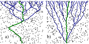
Figure 1: (color online) Paths with lowest energy for given ending states (top, globally optimal path thicker) for (a) the stiff and (b) the tense directed line (right). The dots mark favorable regions of the Gaussian random potential $V$ (realizations of the quenched disorder are not identical in a and b).

The configuration of a general directed line, i.e., one without overhangs or loops and without inextensibility constraint, can be parametrized by $(x,{\bf z}(x))$ $(0\leq x\leq L)$ with a $d$-dimensional displacement ${\bf z}(x)$ normal to its preferred orientation. In the following, we call the fixed projected length $L$ the length of the line. The contour length of the line is given by $L_{c}\approx L(1+\int_{0}^{L}dx\partial_{x}{\bf z}(x))^{2}/2)$ (to leading order in ${\bf z}$); it is not fixed and always larger than the length $L$. Each configuration of a SDL is associated with an energy

$${\cal H} =\int_{0}^{L}\mathrm{d}x\,\left[\frac{\kappa}{2}(\partial_{x}^{2}{\bf z}(x))^{2}+V(x,{\bf z}(x))\right],$$ (1)

where the first term is the bending energy (to leading order in ${\bf z}$). The second term is the disorder energy with a Gaussian distributed quenched random potential $V(x,{\bf z}(x))$ with zero mean $\overline{V}=0$ and short-range correlations

$$\overline{V(x,{\bf z})V(x^{\prime},{\bf z}^{\prime})}=g^{2}\delta^{d}({\bf z}-{\bf z}^{\prime})\delta(x-x^{\prime})$$ (2)

$\overline{X}$ denotes the quenched disorder average over realizations of $V$, whereas ${\langle}X{\rangle}$ denotes thermal averaging.

The SDL model (1) is often used as a weak-bending approximation to the so-called worm-like chain or Kratky-Porod model Harris1966 ; Kratky1949

$${\cal H}_{\text{WLC}} =\int_{0}^{L}\mathrm{d}s\,\left[\frac{\kappa}{2}(\partial_{s}^{2}{\bf r}(s))^{2}+V({\bf r}(s))\right]$$ (3)

which is the basic model for inextensible semiflexible polymers, such as DNA or cytoskeletal filaments like F-actin. The chain is parametrized in arc length, leading to a local inextensibility constraint $\lvert\partial_{s}{\bf r}(s)\rvert=1$, which is hard to account for, both numerically and analytically Kleinert2006 ; Dua2004 . For thermally fluctuating semiflexible polymers, the approximation (1) only applies to a weakly bent semiflexible polymer on length scales below the so-called persistence length, which is Kleinert2006 ; Gutjahr2006

$$L_{p}=\frac{2}{D-1}\frac{\kappa}{T}=\frac{2}{d}\frac{\kappa}{T}.$$ (4)

in $D=1+d$ dimensions. We use here and throughout the following energy units with $k_{B}\equiv 1$. Above the persistence length, a semiflexible polymer loses orientation correlations and starts to develop overhangs.

Also in a quenched random potential the SDL model describes semiflexible polymers in heterogeneous media, only as long as tangent fluctuations are small such that overhangs can be neglected, which is the case below a disorder-induced persistence length, which we will derive below.

We consider the SDL model also in the thermodynamic limit beyond this persistence length, because we find evidence for a relation to the important problem of DLs in a random medium in lower dimensions. This relation is based on replica pair interactions and shows that pair interactions also determine the nature of the DL localization transition. Moreover, this relation can make the DL transition in high dimensions computationally accessible. We will now outline the idea behind this relation.

III Relation to directed lines

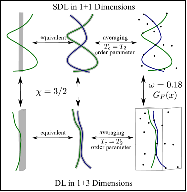
Figure 2: Schematic summary of our findings for the relation between DLs and SDLs. Our results for the energy fluctuation exponent $\omega$ (introduced below in eq. (8)) and for the free energy distribution $G_{F}(x)$ are presented in sections VII.2.1 and VII.3. The shaded area marks the range of the short-ranged (binding) potential. The effective binding interaction becomes apparent in the replica formalism (section V); the importance of two-replica interactions for SDLs is one essential result of this work, see sections VII.4 and VII.5.

The difference between SDLs and DLs HalpinHealy1995 is the second derivative in the first bending energy term in eq. (1) for SDLs, which differs from the tension or stretching energy $\sim\int dx\frac{\tau}{2}(\partial_{x}{\bf z}(x))^{2}$ of DLs with line tension $\tau$. This results in different types of energetically favorable configurations (see Fig. 1): large perpendicular displacements ${\bf z}$ of SDLs as shown in Fig. 1(a) are not unfavorable as long as their “direction” does not change, i.e., as long as their are locally straight and, therefore, do not cost bending energy. Such configurations increase, however, the length of the line and are suppressed for DLs by the tension or stretching energy.

The statistics of displacements ${\bf z}$ is characterized by the roughness exponent $\zeta$, which is defined by $\overline{\langle z^{2}(L)\rangle}\sim L^{2\zeta}$. The thermal roughness is $\zeta_{th,\tau}=1/2$ for DLs and $\zeta_{th,\kappa}=3/2$ for SDLs: equating the thermal energy $T$ with the respective elastic energies gives $T\sim\tau z^{2}/L$ for DLs and $T\sim\kappa z^{2}/L^{3}$ for SDLs. Here and in the following we use subscripts $\tau$ (tension) and $\kappa$ (bending stiffness) to distinguish between the two systems.

Although typical configurations are quite different, a SDL subject to a short-ranged (around $z=0$) attractive potential $V({\bf z})$ can be mapped onto a DL in high dimensions $d^{\prime}=3d$ Bundschuh2000 ; Kierfeld2005 . This equivalence is based on the probability that a free line of length $L$ starting at (${\bf z}(0)=0$) “returns” to the origin, i.e., ends at ${\bf z}(L)=0$. This return probability is characterized by a return exponent $\chi$: $\text{Prob}({\bf z}(L)=0)\sim L^{-\chi}$. The same return exponent characterizes the contact probability $p_{\rm contact}(L)\sim L^{-\chi}$, i.e., the probability of two lines with common starting point to meet again after length $L$, as follows from considering the relative coordinate. For DLs, which are essentially random walks in $d$ transverse dimensions, the return exponent is $\chi_{\tau}=d/2$ Fisher1984 , whereas it is $\chi_{\kappa}=3d/2$ for a SDL (after integrating over all orientations of the end) Gompper1989 ; they are related to the roughness exponents by $\chi=\zeta d$ Kierfeld2005 . The return exponent $\chi$ governs the critical properties of the binding transition to a short-range attractive potential or, equivalently, of the binding transition of two lines interacting by such a potential Bundschuh2000 ; Kierfeld2005 . This follows, for example, directly from a necklace model treatment Fisher1984 . The relation

$$\chi_{\tau}(3d)=\chi_{\kappa}(d)$$ (5)

implies that the binding transition of two DLs in $3d$ dimensions maps onto to the binding transition of two SDLs in $d$ dimensions.

In the replica formulation of line localization problems such as (1), the random potential gives rise to a short-range attractive pair interaction (see below). Therefore, pairwise interactions of DLs play a prominent role also for the physics of a single DL in a random potential. Furthermore, the critical temperature $T_{c,\tau}$ for a DL in a random potential is believed to be identical to the critical temperature $T_{2,\tau}$ for a system with two replicas Monthus2006a ; Monthus2007 . In section VII.4, we will show numerically that also for SDLs in a random medium $T_{c,\kappa}=T_{2,\kappa}$ holds. The important role of pairwise interactions suggests that not only the binding transition of two DLs in $3d$ dimensions maps onto to the binding transition of two SDLs in $d$ dimensions but that the same dimensional relation holds for the localization transitions of DLs and SDLs in a short-range random potential.

One aim of this work is to support this conjecture by providing strong numerical evidence that the $d\rightarrow 3d$ analogy between DLs and SDLs in a random potential holds for the entire free energy distributions for DLs in 1+3 and SDLs in 1+1 dimensions. Because this analogy is rooted in the binding transition of replica pairs, we can conclude that critical properties of the localization transition are determined by pair interactions in the replicated Hamiltonian, which has been previously suggested in Refs. Bundschuh1996 ; Mukherji1996 .

Moreover, it has been proposed that pair interactions can be used to formulate an order parameter of the disorder-driven localization transition of DLs in terms of the overlap $q\equiv\lim_{L\rightarrow\infty}\overline{\frac{1}{L}\int_{0}^{L}\mathrm{d}x\delta(z_{1}(x)-z_{2}(x))}$ Mezard1990 ; Mukherji1994 ; Comets2003 , i.e., the average number of sites per length, that two lines in the same realization of the disorder have in common. Localization by disorder gives rise to a finite value of the pair overlap $q$. This coincides with the binding energy per length that characterizes binding of two polymers by a pair potential. We will also show that the pair overlap indeed provides a suitable order parameter for the localization transition of SDLs in 1+1 dimensions. A schematic summary of the relation of DLs and SDLs together (together with some relevant numeric results) is shown in Fig. 2.

IV Scaling analysis

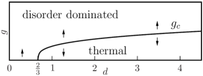
Figure 3: Sketch of the phase diagram as implied by Flory type arguments. The arrows indicate the flow of the disorder “strength” $g$ under renormalization.

IV.1 Lower critical dimension

We start with a scaling analysis by a Flory-type argument. For displacements $\sim z$ the bending energy in eq. (1) scales as $E_{b}\sim z^{2}L^{-3}$, which also leads to $\langle z^{2}\rangle\sim L^{3}/L_{p}$ and the thermal roughness exponent $\zeta_{th,\kappa}=3/2$. The disorder energy in eq.  (1) scales as $E_{d}\sim\sqrt{Lz^{-d}}$, as can be seen from eq. (2). Using the unperturbed thermal roughness in the disorder energy we get $E_{d}\sim L^{(2-3d)/4}$, from which we conclude that the disorder is relevant below a lower critical dimension $d_{c,\kappa}$ with

$$d_{c,\kappa}=2/3.$$ (6)

Above this critical dimension for $d>2/3$ and, thus, in all physically accessible integer dimensions, the SDL should exhibit a transition from a thermal phase for low $g$ to a disorder dominated phase above a critical value $g_{c}$ of the disorder (see Fig. 3). Of course the same distinction could be made in terms of the temperature with a high temperature phase for $T>T_{c}$ and a disorder dominated low temperature phase for $T<T_{c}$. In the disorder dominated phase, the SDL becomes localized or “pinned” into a configuration favored by the random potential and assumes a roughened configuration, see Fig. 1. We remember that the lower critical dimension for DLs is $d_{c,\tau}=2$, which is in accordance with the relation between DLs in 1+3d dimensions and SDLs in 1+d dimensions proposed in the previous section. We also point out that for both types of lines the return exponent $\chi$ assumes the universal value $\chi=1$ at the critical dimension because of $\chi_{\tau}=d_{c,\tau}/2=1$ and $\chi_{\kappa}=3d_{c,\kappa}/2=1$ Bundschuh2000 ; Kierfeld2005 .

With $d_{c,\kappa}=2/3<1$ the localization transition of SDLs can be studied numerically in 1+1 (or higher) integer dimensions, whereas for DLs with $d_{c,\tau}=2$, the localization transition is only accessible in simulations in 1+3 (or higher) integer dimensions. Our numerical study of the line localization transition presented below focuses on SDLs in 1+1 dimensions, which are computationally better accessible using transfer matrix techniques as compared to a 1+3 dimensional system of DLs. This allows us to verify important concepts for the localization transition such as the overlap order parameter in section VII.5, which have not been accessible for DLs in 1+3 dimensions up to now.

IV.2 Roughness

Balancing the Flory estimates, $E_{b}\sim E_{d}$, gives a roughness estimate $z\sim L^{\zeta_{Fl}}$. When disorder is relevant, this leads to

$$\zeta_{Fl,\kappa}=\frac{7}{4+d}~{}~{}\mbox{for}~{}~{}d<d_{c,\kappa}=\frac{2}{3}.$$ (7)

This result is only applicable below the critical dimension $d<d_{c,\kappa}$, where $\zeta_{Fl,\kappa}>\zeta_{th,\kappa}$. Above the critical dimension, the Flory-result would give $\zeta_{Fl,\kappa}<\zeta_{th,\kappa}$, which contradicts our expectation that the SDL roughens as it adjusts to the random potential. Furthermore, the exponent $\omega$ related to the sample to sample free energy fluctuations $\Delta F^{2}\equiv\overline{(F-\overline{F})^{2}}$ via $\Delta F\sim L^{\omega}$ would be negative because of the general scaling relation

$$\omega=2\zeta_{\kappa}-3.$$ (8)

This scaling relation follows from the scaling of the bending energy $E_{b}\sim z^{2}L^{-3}\sim L^{2\zeta_{\kappa}-3}$ and the assumption $\Delta F\sim E_{b}$ that bending and free energy have the same scale dependence. Note that we do not subscript $\omega$ in eq. (8) as we believe that $\omega_{\tau}=\omega_{\kappa}$, see section VII. An exponent $\omega<0$ contradicts the existence of large disorder-induced free energy fluctuations in the low-temperature phase Fisher1991 ; Monthus2006b , for which there is also strong numerical evidenceKim1991 ; Kim1991b ; Monthus2006a . We conclude that this kind of argument is not applicable above the critical dimension. The same problems occur in Flory arguments for the DL for $d>d_{c,\tau}=2$, where one finds $\zeta_{Fl,\tau}=3/(4+d)$ and $\omega=2\zeta_{\tau}-1$. The Flory approach underestimates the roughness exponent for all dimensions both for DLs and SDLs, i.e., $\zeta>\zeta_{Fl}$ as it features only one length scale on which the line can adjust to the disorder. Therefore the Flory results $\zeta_{Fl}$ should provide a lower bound for the roughness exponent, i.e., $\zeta>\zeta_{Fl}$. Moreover, the thermal roughness $\zeta_{th,\tau}=1/2$ for DLs and $\zeta_{th,\kappa}=3/2$ for SDLs should provide another lower bound for the disorder-induced roughness, i.e., $\zeta>\zeta_{th}$ because of the existence of disorder-induced free energy fluctuations in the low-temperature phase, i.e., $\omega>0$.

Furthermore, we can give an upper bound for the disorder-induced roughness by an argument which relates the line to the zero-dimensional problem of a single particle in a harmonic and a random potential Engel1993 . In this argument we divide the line in its middle into two straight and rigid segments separated by the mid-point $(L/2,z)$. The single (i.e. zero-dimensional) coordinate $z$ describes the restricted shape fluctuations of the two-segment line. The bending energy of these shape fluctuations is ${\cal H}_{b}({\bf z})=\frac{1}{2}(\kappa/L^{3})z^{2}$, and the disorder energy of the two straight segments is ${\cal H}_{d}({\bf z})=V({\bf z})$ with $\overline{V({\bf z})}=0$ and $\overline{V({\bf z})V({\bf z}^{\prime})}=(2g^{2}L)\delta^{d}({\bf z}-{\bf z}^{\prime})$. In Ref. Engel1993 , a roughness $\overline{\langle z^{2}\rangle}\sim(g^{2}L)^{1/2}/(\kappa/L^{3})\sim L^{7/2}$ (plus logarithmic corrections) has been obtained for this zero-dimensional problem with the single degree of freedom $z$ by an Imry-Ma argument and a more detailed replica calculation, which implies a roughness exponent

$$\zeta_{0,\kappa}=\frac{7}{4}$$ (9)

for the stiff two-segment line. For the directed line, an analogous argument gives $\zeta_{0,\tau}=3/4$. In the framework of a functional renormalization group (FRG) calculation both roughness exponents can be written as $\zeta_{0}=\epsilon/4$ in a dimensional expansion with the appropriate $\epsilon=4-d$ for DLs and $\epsilon=8-d$ for SDLs (see section VI below). Using the scaling relations (8), this results in $\omega_{0}=\frac{1}{2}$ for two-segment lines (both for SDLs and DLs), which should be considered an upper bound to the energy fluctuation exponent, because the adaptation of the line to the potential must not lead to larger fluctuations as compared to the trivial case of summing up random numbers LeDoussal2004 . Therefore, also $\zeta_{0}$ should provide an upper bound for the roughness exponent, i.e., $\zeta<\zeta_{0}$. The upper bound $\zeta<\epsilon/4$ is also found in the FRG calculation LeDoussal2004 .

All in all, we have obtained bounds

$$\max(\zeta_{th},\zeta_{Fl})<\zeta<\zeta_{0},$$ (10)

which apply both for SDLs and DLs. For SDLs, this gives a relatively small window of possible roughness exponents,

$$\max\left(\frac{3}{2},\frac{7}{4+d}\right)<\zeta_{\kappa}<\frac{7}{4},$$ (11)

which, for example, limits $\zeta_{\kappa}$ for SDLs in 1+1 dimensions to $1.5<\zeta_{\kappa}<1.75$.

V Variation in replica space

To go beyond scaling arguments we use the replica technique Dotsenko2001 following the treatment of directed manifolds by Mezard and Parisi Mezard1991 . For the sake of convenience we restrict ourselves to $d=1$ throughout this section. We will comment on how to adapt this to higher dimensions later on. The quenched average of the free energy $\overline{F}=-\beta^{-1}\overline{\ln Z}$ is treated in the representation

$$\ln Z=\lim_{n\rightarrow 0}n^{-1}(Z^{n}-1)$$ (12)

calculating averages $\overline{Z^{n}}$ of a $n$-times replicated system in the limit $n\to 0$. For the calculation we introduce an additional parabolic potential or “mass” term $\int dx\mu{\bf z}^{2}(x)$ in eq. (1) as an infrared regularization and a finite correlation length $\lambda$ in the disorder correlator,

$$\overline{V(x,z)V(x^{\prime},z^{\prime})}=g^{2}f_{\lambda}((z-z^{\prime})^{2})\delta(x-x^{\prime}),$$ (13)

where we use $f_{\lambda}(x)=\sqrt{2\pi\lambda^{2}}^{-1}\exp{(-x/(2\lambda^{2}))}$ to retain the original $\delta$-correlator (compare eq. 2) for $\lambda\approx 0$. We write the replicated and averaged partition function as $\overline{Z^{n}}=\prod_{\alpha}(\int\mathcal{D}z_{\alpha})\exp{(-\beta{\cal H}_{\text{rep}})}$ with the following replica Hamiltonian in Fourier space

$${\cal H}_{\text{rep}} =\frac{1}{2L}\sum_{\alpha=1}^{n}\sum_{k}(\kappa k^{4}+\mu)z_{\alpha}^{2}$$

$$-\frac{\beta g^{2}}{2}\sum_{\alpha,\beta=1}^{n}\int_{0}^{L}\text{d}x\,f((z_{\alpha}-z_{\beta})^{2}).$$ (14)

As mentioned before, ${\cal H}_{\text{rep}}$ is related to a pair binding problem: in the limit $\lambda\approx 0$ the second term becomes $-\frac{\beta g^{2}}{2}\sum_{\alpha,\beta}\int_{0}^{L}\text{d}x\delta(z_{\alpha}-z_{\beta})$, which is an attractive short-range interaction of two replicated lines.

We use variation in replica space with the quadratic, i.e., Gaussian trial Hamiltonian

$${\cal H}_{V}=(2L)^{-1}\sum_{k}\sum_{\alpha,\beta}z_{\alpha}{G}^{-1}_{\alpha\beta}z_{\beta}$$ (15)

with ${G}^{-1}_{\alpha\beta}=(\kappa k^{4}+\mu)\delta_{\alpha\beta}+{\sigma}_{\alpha\beta}$ with the self-energy matrix $\boldsymbol{\sigma}$ providing variational parameters. Extremizing the lower free energy bound $F\geq F_{V}+\langle{\cal H}_{\text{eff}}-{\cal H}_{V}\rangle_{V}$ with respect to the self-energy matrix $\boldsymbol{\sigma}$ gives (in the continuum limit $L^{-1}\approx 0$) a self-consistent equation for the self-energy matrix Mezard1991

$${\sigma}_{\alpha\beta} =\begin{cases}-\sum_{\alpha^{\prime}\neq\alpha}{\sigma}_{\alpha\alpha^{\prime}}&\alpha=\beta\\ -2\beta g^{2}\tilde{f}^{\prime}\left(({\int}\frac{\text{d}k}{2\pi\beta}({G}_{\alpha\alpha}{+}{G}_{\beta\beta}{-}2{G}_{\alpha\beta})\right)&\alpha\neq\beta\end{cases}$$ (16)

with

$$\tilde{f}_{\lambda}(x)\equiv\int dy\sqrt{2\pi}^{-1}e^{-y^{2}/2}f_{\lambda}(y^{2}x)=\sqrt{2\pi}^{-1}\sqrt{\lambda^{2}+x}^{-1}.$$ (17)

Following Mezard and Parisi we choose a one-step hierarchical replica symmetry breaking Ansatz for $\boldsymbol{\sigma}$. Replica symmetry breaking is relevant here, because there is no nontrivial replica symmetric solution in the limit $\mu\approx 0$ apart from $\sigma_{\alpha\beta}=0$. Furthermore, there is no continuous replica symmetry breaking since $\zeta_{Fl}<\zeta_{th}$ for $d>d_{c,\kappa}$ Mezard1991 . Thus, $\boldsymbol{\sigma}$ can be parametrized by a diagonal element $\tilde{\boldsymbol{\sigma}}$ and a function $\sigma(u)$ ($0\leq u\leq 1)$) giving the non-diagonal elements in the limit $n\rightarrow 0$. For one-step replica symmetry breaking the latter takes the form $\sigma(u)=\sigma_{0}+\Theta(u-u_{c})(\sigma_{1}-\sigma_{0})$. Using the algebra developed by Parisi Parisi1980 and performing the limit of an unbounded system $\mu\rightarrow 0$ we find

$$\sigma_{0} =0$$ (18)

$$\sigma_{1} =-2\beta g^{2}\tilde{f}^{\prime}(\pi S_{1})$$ (19)

with $S_{1}=S_{1}(\Sigma)\equiv\frac{1}{\sqrt{2}\beta}\kappa^{-1/4}\Sigma^{-3/4}$ and $\Sigma\equiv u_{c}\sigma_{1}$. In higher dimensions $d>1$ the stationary equation (16) as well as the result for one-step replica symmetry breaking would be of the same form with different numerical constants, given the functions $f_{\lambda}$ and $\tilde{f}_{\lambda}$ are adapted accordingly, see Parisi1980 . In $d=1$, the variation of the free energy estimate yields two self-consistent equations

$$u_{c}\propto S_{1}(\Sigma)(\lambda^{2}+S_{1}(\Sigma))^{-1}~{}~{}~{}\mbox{and}~{}~{}~{}\Sigma\propto(\beta^{20}g^{16}\kappa^{3}u_{c}^{20})^{-1}$$ (20)

for $u_{c}$ and $\Sigma$, where we omitted numerical constants. We are not able to give a closed solution, because

$$\Sigma^{1/20} \sim\frac{\lambda^{2}+\Sigma^{-3/4}}{\Sigma^{-3/4}}$$ (21)

$$\sim\lambda^{2}\Sigma^{15/20}+\text{const}$$ (22)

Nonetheless, using the condition $u_{c}<1$, we can show that there is no solution unless the potential strength $g$ and correlation length $\lambda$ are above finite values. Although variation in replica space is known Mezard1991 to fail in reproducing the exact solution Kardar1987 for the problem of the DL in disorder in finite dimensions, we interpret this as an indication for the existence of a critical disorder strength or a critical temperature. The replica approach leads, however, to the thermal roughness exponent also in the low-temperature phase.

VI Functional renormalization group

There has been some success studying elastic manifold problems in disordered potentials using functional renormalization group (FRG) analysis Fisher1986 ; Balents1993 ; Chauve2001 ; LeDoussal2002 ; LeDoussal2004 ; LeDoussal2005 . This method can be adapted to generalized elastic energies

$${\cal H}_{m}\sim\int\!\text{d}^{D}\!x\,(\nabla^{m}_{\bf x}{\bf z})^{2}$$ (23)

for $D$-dimensional elastic manifolds with $d$ transverse dimensions (in the FRG literature, the number of transverse dimensions is frequently denoted by $N$). The case $m=1$ corresponds to elastic manifolds as they have been already extensively studied Fisher1986 ; Balents1993 ; Chauve2001 ; LeDoussal2002 ; LeDoussal2004 ; LeDoussal2005 , whereas $m=2$ corresponds to manifolds dominated by bending energy. Lines are manifolds with $D=1$, i.e., DLs correspond to $m=1$ and $D=1$ and SDLs with a bending energy to $m=2$ and $D=1$. In the FRG approach we take the Gaussian distributed random potential to have zero mean and a correlator of the general form

$$\overline{V({\bf x},{\bf z})V({\bf x}^{\prime},{\bf z}^{\prime})} =R({\bf z}-{\bf z}^{\prime})\delta^{(D)}({\bf x}-{\bf x}^{\prime}),$$ (24)

where the whole function $R({\bf z})$ is renormalized under a change of scale.

In renormalization, we integrate out short wavelength fluctuations in a shell $\Lambda/b<|{\bf k}|<\Lambda$ in momentum space and perform a subsequent infinitesimal scale-change (SC) by a factor $b=e^{\mathrm{d}l}$,

$$x \rightarrow bx$$ (25)

$${\bf z} \rightarrow b^{\zeta}{\bf z},$$ (26)

in order to restore the high momentum cutoff $\Lambda$. This leads to the following FRG flow equations

$$\left.\frac{\mathrm{d}T}{\mathrm{d}l}\right|_{\text{SC}} =2(\zeta_{th}-\zeta)T$$ (27)

$$\left.\frac{\partial R}{\partial l}\right|_{\text{SC}} =(\epsilon-4\zeta)R+\zeta(z\cdot\vec{\nabla}_{z})R+{\cal O}(R^{2})+{\cal O}(R^{3})$$ (28)

with

$$\epsilon=4m-D$$ (29)

and $\zeta_{th}=(2m-D)/2$. The flow equation (27) for the temperature is believed to be exact due to a Galilean invariance of the Hamiltonian. For a disorder dominated phase with $\zeta>\zeta_{th}$ corresponding to $\omega>0$, the system is characterized by a $T=0$ RG fixed point, at which we want to determine the roughness exponent $\zeta$.

The terms ${\cal O}(R^{2})$ and ${\cal O}(R^{3})$ in the RG flow equation (28) of the disorder correlation function $R({\bf z})$ are additional one-loop Balents1993 and two-loop Chauve2001 ; LeDoussal2002 ; LeDoussal2004 ; LeDoussal2005 contributions, respectively. In Ref. LeDoussal2004 , a generalized elasticity with a general parameter $m$ has already been discussed up to two-loop level for $d=1$. The one-loop contributions are independent of $m$ and assume exactly the same form for $m=2$ as for standard elastic manifolds with $m=1$ and as they have been calculated in Refs. Fisher1986 ; LeDoussal2002 ; LeDoussal2004 for $d=1$ and Refs. Balents1993 ; LeDoussal2005 for general $d$. For $d=1$, it has been shown that the two-loop contributions, however, acquire a $m$-dependent numerical prefactor LeDoussal2002 ; LeDoussal2004 . For general $d$ and $m$, the two-loop contribution has not been calculated. The exponent $\zeta$ is determined from the FRG equation (28) for $R({\bf z})$ by requiring a fixed point solution for short-range disorder to be positive and vanish exponentially for large $z$. Therefore, in one-loop order results for the roughness exponent $\zeta$ depend on $m$ only through the dimensional expansion parameter $\varepsilon=4m-D$.

For $d=1$, we can adapt the final results achieved in Ref. Fisher1986 in one-loop, which have been extended in Refs. LeDoussal2002 ; LeDoussal2004 to two loops,

$$\zeta_{\rm FRG}=0.20830\varepsilon+0.00686\,X_{m}\,\varepsilon^{2}$$ (30)

with the $m$-dependent numerical prefactor $X_{m}$ ($X_{1}=1$, $X_{2}=-1/6$ to leading order in $\varepsilon$). For a SDL ($D=1$, $m=2$, $\epsilon=7$) with $d=1$ transverse dimensions, we obtain a roughness exponent $\zeta_{{\rm FRG},\kappa}\approx 1.4571$ in one-loop, which is close to the Flory estimate $\zeta_{Fl,\kappa}=\frac{7}{5}$ but also violates the lower bound set by the thermal roughness, $\zeta_{{\rm FRG},\kappa}<\zeta_{th,\kappa}=3/2$, implying $\omega<0$. On the two-loop level, we find a negative prefactor $X_{2}<0$ and, thus, still $\zeta_{{\rm FRG},\kappa}<\zeta_{th,\kappa}=3/2$.

In the literature, the existence of an upper critical dimension $d_{u}$, above which $\zeta<\zeta_{th}$ applies, has been discussed, in particular for DLs ($D=1$, $m=1$) and as a candidate for the upper critical dimension of the KPZ equation to which the DL problem can be mapped. Our above finding $\zeta_{{\rm FRG},\kappa}<\zeta_{th,\kappa}=3/2$ in two-loop order indicates that for SDLs with $m=2$, $d=1$ is already above the upper critical dimension $d_{u,\kappa}$, i.e., $d_{u,\kappa}<1$. Using the one-loop result for general $d$, we can estimate this upper critical dimension $d_{u,\kappa}$ for SDLs. The approximate formula

$$\zeta_{\rm FRG}(d)=\frac{\varepsilon}{4+d}\left(1+\frac{1}{4e}2^{-(d+2)/2}\frac{(d+2)^{2}}{d+4}\right)$$ (31)

from Ref. Balents1993 gives a critical dimension $d_{u,\kappa}=0.937669<1$. Solving the FRG fixed point equation for $R({\bf z})$ numerically, we find $d_{u,\kappa}\approx 0.84<1$ using the one-loop equations and the numerical methods outlined in LeDoussal2004 (we use Taylor expansions up to order $12$, which allows us to determine $\zeta$ to four digits). The result $d_{u,\kappa}<1$ remains valid using the two-loop equations, where the additional two-loop terms contain the same factor $X_{m}$ as for $d=1$. However, the two-loop result for the critical dimension is lower because, analogously to the DL results of Ref. LeDoussal2005 , the two-loop corrections are negative for $d>d_{u,\kappa}$. In the following section, we present numerical results which show that there exists a disorder dominated phase with $\zeta_{\kappa}>\zeta_{th,\kappa}=3/2$ for SDLs in $d=1$ below a critical temperature, which shows that the FRG results are questionable for lines with $D=1$ and, correspondingly, large values for the expansion parameter $\epsilon$.

VII Numerical results

Returning from (D+d)-dimensional manifolds to the problem of (1+d)-dimensional SDLs in disorder, further progress is possible by numerical studies using the transfer matrix method HalpinHealy1995 ; Wang2000 both for $T=0$ (see Fig. 1) and for $T>0$.

Previous numerical studies for DLs in 1+3 dimensions offer the opportunity for a comparison of the exponents $\omega$ (energy fluctuations), describing the low temperature phase, and $\nu$ (correlation length), describing the transition, in the low temperature phase to test the aforementioned analogy to a SDL in 1+1 dimensions. The values found there are $\omega\approx 0.186$ Kim1991b ; Ala1993 ; Monthus2006a ; Marinari2000 and either $\nu\approx 2$ Monthus2006a ; Monthus2007 ; Derrida1990 or $\nu\approx 4$ Monthus2006a ; Kim1991 .

VII.1 Transfer matrix algorithm

From a discretization of the energy functional given in eq. 1 we conclude that a segment of a SDL with length $\Delta L=1$ starting at $z$ with orientation $\text{d}z/\text{d}x=v$ and ending at $z^{\prime}$ with orientation $v^{\prime}$ contributes an energy

$$\Delta E_{x}(v-v^{\prime},z^{\prime})=\frac{\kappa}{2}(v-v^{\prime})^{2}+V(x,z^{\prime}),$$ (32)

where the additional condition $z^{\prime}=z+v$ applies which connects positions and tangents. We will also exploit the quadratic behavior in $v-v^{\prime}$ and only consider segments with $(v-v^{\prime})^{2}\leq\Delta_{v}^{2}$ with a constant $\Delta_{v}>1$ in the partition sum. The random potential $V(x,z)$ is represented by Gaussian random variables Marsaglia2000 with $\overline{V(x,z)}=0$ and $\overline{V(x,z)V(x^{\prime},z^{\prime})}=g^{2}\delta_{xx^{\prime}}\delta_{zz^{\prime}}$. For the sake of simplicity and comparability we choose $g=1$ and vary the temperature. Unless stated differently we set $\kappa=5$ and $\Delta_{v}=5$ and simulate lengths up to $L=100$ using, in principle, all intermediate lengths and at least $10^{4}$ realizations of the disorder.

VII.1.1 Zero temperature

For vanishing temperature $T=0$ there are no entropic contributions to the free energy. Hence the line is always in its ground state and minimizing the energy $E_{L}^{0}$, where the subscript denotes the length and the superscript is a reminder that these considerations are valid for $T=0$. This can be done iteratively

$$E_{L}^{0}(z^{\prime},v^{\prime}) {=}\min_{v}\left[E^{0}_{L-1}(z^{\prime}{-}v,v)+\Delta E_{L}(v{-}v^{\prime},z^{\prime})\right]$$ (33)

and all quantities $X$ are to be measured in the resulting (non-degenerate) ground state

$$\langle X\rangle_{T=0} =X(z_{\text{min}},v_{\text{min}})$$ (34)

with $E^{0}_{L}(z_{\text{min}},v_{\text{min}})=\min_{z,v}E^{0}_{L}(z,v)$.

VII.1.2 Finite temperature

At finite temperatures $T>0$, the restricted partition function $Z_{L}(z,v)=\int_{z(0)=v(0)=0}^{z(L)=z,v(L)=v}{\cal D}z\exp{(-\beta{\cal H})}$ has to be evaluated. We are using the transfer matrix approach and divide the line into straight segments which are connected by the transfer matrix. This allows for an iterative computation of the restricted partition function

$$Z_{L}(z^{\prime},v^{\prime}) =\!\!\!\!\!\sum_{\begin{subarray}{c}v,\\ \!z=z^{\prime}-v\!\end{subarray}}\!\!\!\!\exp{({-}\beta\Delta E_{L}(v{-}v^{\prime},z^{\prime}))}Z_{L-1}(z,v);$$ (35)

for numerical stability reasons, the $Z_{L}(z,v)$ are normalized in each length iteration such that $\sum Z_{L}(z,v)=1$. The normalization constant is a useful quantity as it is the total partition function and therefore gives the free energy. Additionally, the normalized restricted partition function is used in the computation of thermal averages

$$\langle X\rangle=\left(\sum_{z,v}Z_{L}(z,v)\right)^{-1}\sum_{z,v}X(z,v)Z_{L}(z,v)$$ (36)

This averaging procedure is only correct for quantities $X$ that are measured at the end of the line, moments of the energy (potential or total) are accumulated along the contour of the line and have, therefore, to be computed in an iteration scheme Wang2000 very similar to eq. (35). Finally, for all observables the quenched average over realizations of the disorder has to be performed.

VII.2 Existence and nature of the disorder dominated phase

VII.2.1 Roughness

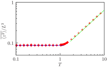
Figure 4: The roughness $\overline{\langle z^{2}\rangle}$ as a function of the temperature. There are two distinct regimes where the roughness scales as $\overline{\langle z^{2}\rangle}\sim T^{0}$ and $\overline{\langle z^{2}\rangle}\sim T$ respectively. We plotted these asymptotics as well. We show lengths $L=50,60,\ldots,100$, so that the “scattering” of the symbols for one temperature indicate the quality of the rescaling with $L^{-3}$ (see also Fig. 5).

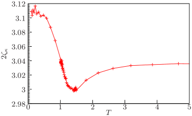
Figure 5: (color online) Roughness exponent $2\zeta_{\kappa}$ for various temperatures, computed via (37). The deviation for high temperatures from the analytical value $2\zeta=3$ indicates numerical shortcomings, nonetheless there is a clear “dip” at $T\approx 1.4$, which we identify as the critical temperature. For low temperatures, we find values consistent with $\omega\approx 0.11$.

The most natural observable to analyze looking for a localization transition is the roughness $\overline{\langle z^{2}\rangle}$. One expects to see two different regimes, a high temperature phase with the thermal roughness $\overline{\langle z^{2}\rangle}\sim TL^{3}$ and a low temperature phase with $\overline{\langle z^{2}\rangle}\sim T^{0}L^{2\zeta}$. Also, the influence of numerical details onto the roughness should be smaller than their influence on the free energy. Figure 4 shows the roughness $\overline{\langle z^{2}\rangle}$ as a function of temperature and demonstrates that these expectations are met. In order to determine the roughness exponent $\zeta_{\kappa}$ we measure a “local” roughness exponent Schwartz2012

$$2\zeta(L)=\log_{5}(z^{2}(L)/z^{2}(L/5))$$ (37)

The data for $\zeta_{\kappa}$ as a function of temperature presented in Fig. 5 exhibits two distinct high and low temperature regimes and a significant “dip” of the local roughness exponent around $T\approx 1.4$. This method of determining $\zeta$ gives better results than fitting $\overline{\langle z^{2}\rangle}(L)$

Via the scaling relation (8), $\omega=2\zeta_{\kappa}-3$, we obtain the exponent $\omega$ from the roughness exponent $\zeta_{\kappa}$. As in the context of DLs Doty1992 , it can be argued that $\omega$ should vanish at the disorder-induced localization transition, resulting in a roughness exponent $\zeta_{\kappa}=3/2$. This seems to hold, even though the numerical value for high temperatures is slightly above $\zeta_{\kappa}=3/2$. This is strong evidence for a phase transition at $T_{c}\approx 1.4$. For low temperatures, the values $2\zeta_{\kappa}\approx 3.11$ give $\omega\approx 0.11$ according to eq. (8), which is slightly lower than $\omega=0.186$, which is the literature value for DLs in 1+3 dimensions Kim1991b ; Ala1993 ; Monthus2006a ; Marinari2000 .

VII.2.2 Disorder-induced persistence length

The roughness is closely related to the averaged tangent directions $\overline{\langle v^{2}\rangle}\equiv\overline{\langle(\partial_{x}z)^{2}\rangle}$, which should scale as

$$\overline{\langle v^{2}\rangle}\sim\overline{\langle z^{2}\rangle}/L^{2}\sim L^{2(\zeta-1)}\sim L^{1+\omega}.$$ (38)

We define an effective disorder-induced persistence length $\tilde{L}_{p}$ for the SDL as the length scale at which the tangent fluctuations become equal to one

$$\overline{\langle v^{2}\rangle}(\tilde{L}_{p})=1.$$ (39)

This generalized definition for the disordered system is consistent with the standard definition for the persistence length $L_{p}$ of a thermally fluctuating SDL in the absence of disorder, where we expect $\overline{\langle v^{2}\rangle}\approx L/L_{p}$ with $L_{p}=\beta\kappa$. Apart from numerical prefactors this gives the standard persistence length of the WLC model, see eq. (4), which is defined as the decay length of tangent correlations.

In the low temperature phase, we expect a disorder dominated roughness and, therefore, temperature-independent tangent fluctuations $\overline{\langle v^{2}\rangle}$, which results in a temperature-independent disorder-induced persistence length $\tilde{L}_{p}\sim\beta^{0}$. The line roughens in the low temperature phase, which gives rise to a persistence length decrease as compared to the thermal persistence length $L_{p}\sim\kappa/k_{B}T$. From the Flory-result $z\sim(g/\kappa)^{2/(4+d)}L^{7/(4+d)}$ at low temperatures, we expect $v\sim(g/\kappa)^{2/(4+d)}L^{(3-d)/(4+d)}$ for the disorder-induced tangent fluctuations and

$$\tilde{L}_{p}\sim(\kappa/g)^{2/(3-d)}$$ (40)

at low temperatures according to the criterion (39). For SDLs in 1+1 dimension, we expect $\tilde{L}_{p}\propto g^{-1}$.

To determine the generalized persistence length from eq. (39) numerically, we used the tilt symmetry of the replicated Hamiltonian Giamarchi1995 , according to which the “connected” average

$$\overline{\langle v^{2}\rangle-\langle v\rangle^{2}}\approx L/\beta\kappa$$ (41)

is independent of the disorder strength. Therefore, we can use a fit to the sample-to-sample tangent fluctuations of the form

$$\overline{\langle v\rangle^{2}}(T,L)=a(T)L^{1+\omega^{\prime}(T)}$$ (42)

with an amplitude $a(T)$ and an exponent $\omega^{\prime}(T)$, which should agree with the free energy exponent $\omega$. Then, we can rewrite $\overline{\langle v^{2}\rangle}$ as

$$\overline{\langle v^{2}\rangle} =\overline{\langle v^{2}\rangle-\langle v\rangle^{2}}+\overline{\langle v\rangle^{2}}$$

$$=L/\beta\kappa+a(T)L^{1+\omega^{\prime}(T)},$$ (43)

and determine $\tilde{L}_{p}$ using eq. (39). Our results for $\tilde{L}_{p}$ are shown in Fig. 6. In the low-temperature phase for $T<T_{c}\approx 1.4$, the persistence length becomes indeed disorder-induced, i.e., almost independent of temperature and our results are consistent with the above scaling result (40). We consider this non-divergent persistence length at low temperatures also to be consistent with previous results for the non-directed version of the SDL, the WLC in disorder Dua2004 . In the high temperature phase, our results approach the standard thermal persistence length $L_{p}\sim\beta\kappa$.

The fit results for $a(T)$ and $\omega^{\prime}(T)$ are shown in Fig. 7. For $T<T_{c}$ our results are consistent with $\omega\approx 0.186$, which is the literature value for DLs in 1+3 dimensions Kim1991b ; Ala1993 ; Monthus2006a ; Marinari2000 . In fact, we get very similar results for $L_{p}$ if we fix $\omega^{\prime}(T)=\omega=0.186$.

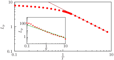
Figure 6: (color online) The generalized persistence length $\tilde{L}_{p}$ according to eqs. (39) and (43) as a function of the temperature $T$. (43). $\tilde{L}_{p}$ matches its thermal value (solid line) for $T>T_{c}$ and is reduced and approximately constant for $T<T_{c}$. Inset: $\tilde{L}_{p}$ at $T=0$ versus the potential strength $g$. The Flory-result $\tilde{L}_{p}\sim g^{-1}$ (dotted line), see eq. (40) matches the data.

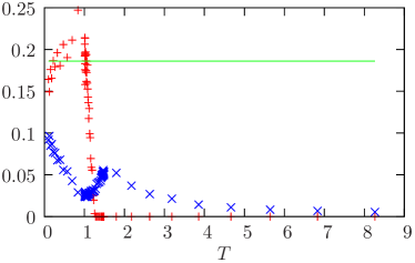
Figure 7: (color online) Parameters $a(T)$ (blue, Greek crosses) and $\omega^{\prime}(T)$ (red, saltires) used in fitting $\overline{\langle v\rangle^{2}}$, cf. eq. 42. The latter vanishes around, but not exactly at $T=T_{c}$. The horizontal line corresponds to the literature value for DLs in 1+3 dimensions, $\omega=0.186$.

VII.2.3 Derrida-Flyvbjerg singularities

One of the features expected in a disorder dominated phase are Derrida-Flyvbjerg singularities Derrida1987 ; Monthus2007b . These are features of the statistical weights, here the normalized restricted partition $w(z)=Z(z)/Z$ function for the SDL to end at a specific point $z$. As the phase is disorder dominated, some characteristics of these weights should origin from mere statistics and the distribution used for the random potential rather than details of the Hamiltonian involved. According to Derrida and Flyvbjerg the distributions $P_{1}(w_{1})$ and $P_{2}(w_{2})$ of the largest and the second largest weight, respectively, should exhibit singularities at $1/n$ ($n=1,2,3,...$) in a disorder dominated phase with a multivalley structure of phase space Derrida1987 . For SDLs in disorder, we calculated the distribution of the value of the largest and the second largest weight numerically as shown in Fig. 8 and indeed find singularities at $1$ and $1/2$ for $T<T_{c}$. We are not able to clearly resolve higher singularities at $1/n$ with $n\geq 3$, which might be due to the underlying (Gaussian) distribution or the number of samples used. Analogous singularities can be found in the distribution of the information entropy $s=-\sum_{z}w\ln w$ at values $-\ln(1),-\ln(2),-\ln(3)$, whereas nothing similar can be observed at high temperatures, where the entropy distribution is Gaussian and the distribution of the (second) largest weight is sharply peaked around zero. We see this as a confirmation that the SDL indeed undergoes a transition to a disorder dominated phase At $T_{c}\approx 1.4$.

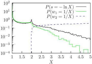
Figure 8: (color online) Distribution of the largest ($w_{1}$, light (green) solid line) and second largest ($w_{2}$, (blue) dashed line) statistical weight $w(z)=Z(z)/Z$ and the information entropy $s=-\sum_{z}w(z)\ln{w(z)}$ (black, dark solid line).

VII.3 The free energy distributions of SDL in 1+1 and DL in 1+3 dimensions are identical

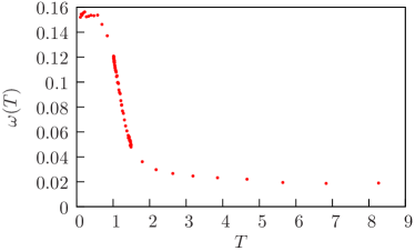
Figure 9: (color online) Fluctuation exponent $\omega$ determined by the free energy fluctuations.

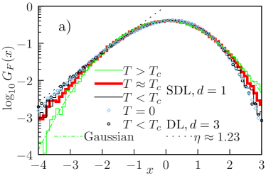
Figure 10: (color online) Rescaled $G_{F}(X)=P((F-\overline{F})/\Delta F)$ free energy distribution for a stiff directed line (SDL) in 1+1 dimensions. We show distributions for $T=0$ (light (blue) squares, ground state energy) as well as for three finite temperatures $T<T_{c}$ (black thin solid line), $T\approx T_{c}$ (red, thicker solid line) and $T>T_{c}$ (green, light thin solid line). Results for a directed line (DL) in 1+3 dimensions are shown (dark circles).

The exponent $\omega$ can alternatively be determined in a more direct way by fitting $\Delta F=({\overline{F^{2}}-\overline{F}{}^{2}})^{1/2}\propto L^{\omega}$ at temperatures $T\ll T_{c}$, giving values of $\omega\approx 0.15-0.16$ (cf. Fig. 9).

We can go one step further and consider not only the second moment but the whole distribution of the free energy as shown in Fig. 10, which is obtained by computing the free energy for every sample and rescaling to zero mean and unit variance,

$$G_{F}(X)=\text{Prob}((F-\overline{F})/\Delta F=X).$$ (44)

This rescaling should make $G_{F}$ more robust against the influence of numerical details. For DLs in $d=1$ it has been found that this distribution is of a universal form Dotsenko2011 . The asymptotic behavior of the negative tail of the rescaled free energy distribution for low temperatures is of the form

$$\ln{G_{F}(X)} \sim-\lvert X\rvert^{\eta}\quad(X<0,\lvert X\rvert\gtrapprox 1).$$ (45)

This allows us to determine the energy fluctuation exponent $\omega$ via the Zhang argument HalpinHealy1995 ; Monthus2006a ; Monthus2006c : a saddle point integration gives $\ln\overline{Z^{n}}\sim-n\overline{F}/T-(n\Delta F/T)^{\eta/(\eta-1)}$; on the other hand, $\ln\overline{Z^{n}}\sim L$ should be extensive resulting in $\Delta F\sim L^{1-1/\eta}$ or

$$\eta=(1-\omega)^{-1}.$$ (46)

We find $\eta\approx 1.23$ (dashed black line in Fig. 10) or $\omega\approx 0.18$. This is in agreement with the values reported for DLs in 1+3 dimensions.

For a direct comparison of the rescaled free energy distributions of a SDL in 1+1 and a DL in 1+3 dimensions we simulated both systems (the DL up to lengths $L=60$) and find that the rescaled free energy distributions in the low temperature phases have to be considered identical within numerical accuracy. This could hint towards a new seemingly “universal” distribution for certain random systems, much like the Tracy-Widom distribution that is found for the DL in 1+1 dimensions and various other systems Dotsenko2011 . For finite system sizes this universal behavior can only be expected for free energy fluctuations $\lvert X\rvert$ small compared to an upper threshold Kolokolov2007 ; Kolokolov2008 ; we believe, however, that our simulation does not cover the very rare fluctuations that induce the non-universal part for very large $\lvert X\rvert$. In Fig. 11 we show the distributions for $T<T_{c}$ (DL and SDL) in a manner where the exponent $\eta$ becomes more apparent. Here we introduce the exponent $\eta^{\prime}$, which is the analogon to $\eta$ for the positive tail

$$\ln{G_{F}(X)} \sim-\lvert X\rvert^{\eta^{\prime}}\quad(X>0,\lvert X|\gtrapprox 1),$$ (47)

where the Zhang argument is not applicable. We find a value $\eta^{\prime}\approx 1.84$.

Based on an exact renormalization on the diamond lattice Monthus2008 and an optimal fluctuation approach Kolokolov2008 , it has been previously suggested for DLs that $\eta^{\prime}$ and $\omega$ are related via (cf. eq.  (46))

$$\eta^{\prime} =d_{\text{eff}}/(1-\omega)$$ (48)

with $d_{\text{eff}}=1+d$ for the hypercubic lattice. This is found to be valid for the DL in 1+1 dimensions, where $\omega=1/3$ and $\eta^{\prime}=3$ (Monthus2008, , and references cited therein). For the problem at hand, the literature value $\omega=0.186$ for DLs in $d=3$ would lead to $\eta^{\prime}\approx 5$, which is far from the value $\eta^{\prime}\approx 1.84$ we find; thus, the ratio $\eta^{\prime}/\eta$ does not match the prediction $\eta^{\prime}/\eta=(1+d)$. In Ref. Kolokolov2008 $\eta=2$ and $\eta^{\prime}=3$ were found to be superuniversal (independent of $d$) for the DL in dimensions $d>2=d_{c}$ at temperatures $T>T_{c}$. We can neither confirm nor deny this result, as we are not able to cover the “most distant” part of the distribution, but our interpretation that $G_{F}$ is Gaussian for $T>T_{c}$ would lead to $\eta=\eta^{\prime}=2$.

The finite size corrections to the free energyHalpinHealy1995 ; Krug1990 should also scale as $L^{\omega}$ leading to

$$F/L \approx a+bL^{\omega-1}$$ (49)

We did not succeed in determining a precise, consistent $\omega$ in this way, possibly because our systems are too small.

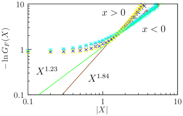
Figure 11: (color online) Double logarithmic plot of the negative logarithm of the rescaled free energy distribution $G_{F}(X)$ ($X=(F-\overline{F})/\Delta F$) at low temperatures $T<T_{c}$ for the DL (light blue stars for $X<0$ and yellow squares for $X>0$) and the SDL (red Greek crosses for $X<0$ and dark blue saltires for $X>0$). We see identical behavior for SDL and DL consistent with exponents $\eta\approx 1.23$ and $\eta^{\prime}\approx 1.84$, see text.

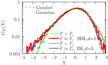
Figure 12: Rescaled potential energy distribution for a SDL in 1+1 dimensions. Plotted are distributions for three finite temperatures $T<T_{c}$ (black, dark thin solid line), $T\approx T_{c}$ (red, thick solid line) and $T>T_{c}$ (green, light solid line). Results for a DL in 1+3 dimensions are shown in blue (medium solid line). Here, the brown (dark dashed) curve is an approximation using a one-parameter Gumbel distribution (cf. eq. (52a) with $m=1.7$), whereas the yellow (light dashed) curve is the normal distribution.

The free energy distributions in Fig. 10 seem to be identical for $T<T_{c}$ and $T\approx T_{c}$ (as it is also the case for the DL Monthus2006a ), which suggests $\omega_{T=T_{c}}=\omega_{T<T_{c}}\approx 0.186$ contradicting the $\omega_{T=T_{c}}=0$ argument Doty1992 , but one has to bear in mind that the saddle point integration in the course of the Zhang argument is only applicable if $\eta>1$ or $\omega>0$.

A more distinct difference between the behavior at criticality and at low temperatures can be found in the distribution of the potential energy as shown in Fig. 12 (also the potential energy is rescaled using $X=(E-\overline{E})/\Delta E$ analogously to Fig. 10 for the free energy distribution). For the potential energy distribution, the behavior at the critical temperature is clearly different from the behavior both at $T>T_{c}$ and $T<T_{c}$ (which are not identical for the DL) and exhibits a decay

$$\ln{G_{E}(X)}\sim\exp{(-|X|)}\quad(X<0,\lvert X|\gg 1).$$ (50)

resembling extreme value distributions of the Gumbel type.

A tentative explanation might be that the transition occurs because of extreme values of the potential at which the otherwise thermally fluctuating line localizes. The random potential has a Gaussian distribution, thus its extreme values are distributed according to a Gumbel distribution or Fisher-Tipett type I extreme value distribution Gumbel1954

$$P^{\alpha,\beta}_{\text{Gumbel}}(X) =\frac{1}{\beta}e^{-z(X)-e^{-z(X)}},$$ (51)

with $z(X)=(X-\alpha)/\beta$, the location parameter $\alpha$, and the scale parameter $\beta$ (the parameters depend on the number of “trials”). The distribution of the potential energy at the critical temperature might be of a similar shape. As we are studying the rescaled distribution of the potential energy, which has zero mean and unit variance, we can use a one-parameter version of the Gumbel distribution

$$g_{m}(X) =\frac{\psi_{1}(m)m^{m}}{\Gamma(m)}\exp{\left(h_{m}(X)-\mathrm{e}^{h_{m}(X)}\right)}^{m}$$ (52a)

with the shape parameter $$m$$, the abbreviation

$$h_{m}(X) \equiv(X+\psi(m))\psi_{1}(m)-\ln{m}$$ (52b)

and the usual $\Gamma(m)=\int_{0}^{\infty}\mathrm{d}t\,t^{m-1}\mathrm{e}^{-t}$ (gamma function), $\psi(m)=\mathrm{d}\ln{\Gamma(m)}/\mathrm{d}m$ (digamma function) and $\psi_{1}(m)=\mathrm{d}^{2}\ln{\Gamma(m)}/\mathrm{d}m^{2}$ (trigamma function) Abramowitz1972 . This distribution inherently features the correct decay at the tails, with $\ln{g_{m}(X)}$ decreasing faster than algebraic for $X<0$ and linearly with slope $m\psi_{1}(m)$ for $X>0$. However, our best approximation to the data with $m=1.7$ deviates for $X>0$. It is remarkable that the potential energy distribution is well described by an extreme value distribution only right at the transition at $T=T_{c}$, whereas it approaches a Gaussian not only for $T>T_{c}$ but also for $T<T_{c}$, see Fig. 12. The Gaussian distribution at low temperatures might stem from the Gaussian distribution used in the realization of the disorder potential.

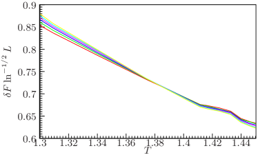
Figure 13: (color online) The reduced free energy $\delta F=\overline{F}-\overline{F}_{\text{ann}}$ rescaled by $\ln^{1/2}{L}$ for lengths $L=50,60,\ldots,100$ as a function of the temperature $T$. There is a pseudo-crossing of the lines around $T\approx 1.38$.

At the critical temperature, where $\omega\approx 0$, the fluctuations of the free energy have been found to scale logarithmically with $L$, $\Delta F\sim\ln^{1/2}{L}$ Monthus2006a . We support this statement by studying the difference of quenched and annealed free energies $\delta F=\overline{F}-\overline{F}_{\text{ann}}$, which should as well scale as $\delta F\sim\ln^{1/2}{L}$ at the transition. As the annealed free energy directly depends numerical details such as system size and neglected elements of the transfer matrix, we determine it by simulating a system without disorder and adding the contribution of the annealed potential, $\overline{F}_{\text{ann}}=F_{g=0}-Lg^{2}\beta/2$. This also allows for an approximate determination of the critical temperature by finite size scaling, see Fig.  13. To verify this argument we tried also different scaling behaviors of the form $\delta F\sim\ln^{c}{L}$ and obtained a consistent pseudo-crossing only for $c\approx 1/2$. Furthermore the annealed free energy can be used to compute the temperature $T_{0,\kappa}$, below which the annealed entropy is negative. This provides a lower bound on the actual critical temperature, whereas the replica pair binding temperature $T_{2,\kappa}$ represents an upper bound Monthus2006a . We find $T_{0,\kappa}\approx 0.4$, which is consistent with $T_{c}\approx 1.4$.

VII.4 The localization transition temperature $T_{c}$ equals the replica pair transition temperature $T_{2}$ for SDLs

We have checked for the SDL via numerical transfer matrix calculations that the localization temperature in disorder $T_{c,\kappa}$ equals transition temperature $T_{2,\kappa}$ for replica pair binding, $T_{c,\kappa}=T_{2,\kappa}$. As stated before, we use the same transfer matrix algorithm for the replica pair system with a short-range binding potential by exploiting that the binding of two SDLs can be rewritten as a binding problem of one effective SDL in an external potential using relative coordinates Kierfeld2003 . This SDL has a bending stiffness of $\kappa^{\prime}=\kappa/2$ and the “potential energy” we are interested in (cf. eq. (14)) for the replica pair binding is $-\beta g^{2}\int\text{d}x\delta(z)$. For the interpretation of the simulation results one has to keep in mind that the energy functional is temperature dependent and, therefore, derivatives of the free energy with respect to the inverse temperature $\beta$ are not given directly by cumulants of the internal energy. Using $E_{b}=\int\text{d}x(\partial^{2}_{x}z)^{2}$ and $V=-g^{2}\int\text{d}x\delta(z)$ the partition function is given by $Z=\int\mathcal{D}z\exp{(-\beta E_{b}-\beta^{2}V)}$ and the free energy by $F=-\beta^{-1}\ln Z$ implying that

$$\frac{\partial(\beta F)}{\partial\beta} =\langle E_{b}+2\beta V\rangle=U+\beta\langle V\rangle$$ (53)

where $U$ is the total internal energy (treating $\beta V$ as a potential). Thus, the derivative of the difference of the free energies with and without the adsorption term with respect to the inverse temperature, which should give the divergent correlation length $\beta\delta F=F_{V}-F_{0}\sim L(T_{c}-T)^{\nu}$, is identical to the “potential energy” $E_{pot}=-\beta V$ and usual finite size scaling should be applicable, cf. Fig. 14. We retain the known correlation length exponent $\nu=2$ for the adsorption problem Kierfeld2003 . We see matching curves for the used system sizes $L=100,200\ldots 500$ around $T-T_{c}\approx 0$ for $T_{2,\kappa}=1.44$, which equals $T_{c,\kappa}\approx 1.4$ for the SDL in disorder.

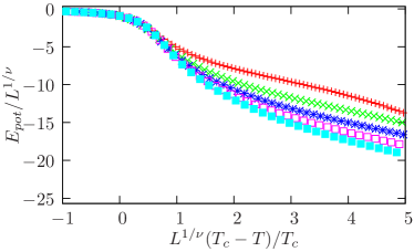
Figure 14: (color online) Finite size scaling for the SDL adsorption problem that corresponds to the two-replica binding, see text for detailed explanation. The scaling uses $T_{c}=1.44$ and $\nu=2$. As only one sample is needed for the calculation we used larger system lengths $L=100$ (red, Greek crosses),$200$ (green, saltires),…,$500$ (light blue, full squares).

VII.5 Pair overlap as order parameter

Finally, we identify an order parameter of the localization transition. For DLs, the disorder-averaged overlap $q=\lim_{L\rightarrow\infty}\overline{\frac{1}{L}\int_{0}^{L}\mathrm{d}x\delta(z_{1}(x)-z_{2}(x))}$ of two replicas has been proposed as order parameter Mezard1990 ; Mukherji1994 . Up to now, it has been numerically impossible to verify this order parameter for DLs in $d>2$ dimensions where a localization transition exists because the relevant $2d$-dimensional two replica phase space is too large. For SDLs, on the other hand, the transition is numerically accessible already in 1+1 dimensions and we show that the overlap $q$ is indeed a valid order parameter using an adaptation of the transfer matrix technique from Ref. Mezard1990 , see Fig. 15. This involves simulating two interacting SDLs, therefore we can only use lengths up to $L=30$ and $10^{3}$ samples. For DLs, it has been found that the overlap at criticality decays as $q\sim L^{\Sigma}$ with $\Sigma=-2\zeta=-(1+\omega)$ in $d=3$ Mukherji1994 . This has been extended to finite temperatures yielding $q\sim\lvert T-T_{c}\rvert^{-\nu\Sigma}$. Indeed, we find a qualitatively similar behavior $q\sim\lvert T-T_{c}\rvert^{-\beta^{\prime}}$ with an exponent $\beta^{\prime}\approx 1.3-1.4$. Our best estimate for $\Sigma$ is $\Sigma\approx-0.75$, cf. Fig. 16. Because of small simulation lengths $L$ we do not conclude this deviation to be a definite statement against the renormalization group results presented in Ref. Mukherji1994 , but this would, unlike the DL renormalization group result $\Sigma=-(1+\omega)$, suggest that two SDLs in a random potential are certain to meet eventually Fisher1984 . For the correlation length exponent $\nu$ we find values $\nu\approx 2$ compatible with the corresponding problem of DLs Monthus2006a ; Monthus2007 ; Derrida1990 ; such that our present results deviate from $\beta^{\prime}=\nu\Sigma$. Nevertheless, the connection between DLs and SDLs provides the first system to test the proposed order parameter in a localization transition numerically and to determine the otherwise inaccessible exponents $\beta^{\prime}$ or $\Sigma$.

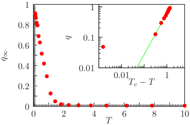
Figure 15: (color online) Overlap order parameter $q$, as a function of $T$. We estimate $q$ from finite lengths using a fit $q_{T}(L)=a(T)/L+q_{\infty}(T)$. Inset: Double-logarithmic plot of the overlap $q$ versus $T_{c}-T$ (with $T_{c}=1.44$), the solid line is given by $q\sim(T_{c}-T)^{-\beta^{\prime}}$ with $\beta^{\prime}\approx-1.36$.

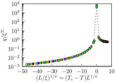
Figure 16: (color online) Finite size scaling ($L=15,\ldots,30$) for the overlap order parameter. Our best results are $\Sigma\approx 0.75$ for the exponent related to the decay of the order parameter, and $\nu\approx 2$ for the correlation length exponent. As before, we used $T_{c}=1.44$.

VII.6 Multifractal properties at the transition

For DLs in 1+3 dimensions, some insight into the underlying structure of the transition has been achieved within the multifractal formalism Jensen1987 . As we conjecture the transitions for the DL and SDL to be essentially analogous, we expect to find similarities to the analysis that has been done before for DLs Monthus2007 , but also deviations where the obvious geometrical differences become important. The idea is that different moments $Y_{q}$ of the statistical weights

$$Y_{q}(L)=\sum_{i}\text{Prob}(z(L)=z_{i})^{q}$$ (54)

are dominated by different regions of the support and thus show a different scaling with the system size $L$. The probability is given by the ratio of restricted and unrestricted partition function $\text{Prob}(z(L)=z_{i})\equiv w_{L}(z_{i})=Z_{L}(z_{i})/Z_{L}$. The sum goes over all the possible ending points in the numerical simulation, whereas for the continuous analytical problem $Y_{q}$ would be defined by an integral over $z$.

In the high temperature phase, the weights $w_{L}(z)$ obey the scaling form $w_{L}(z)=L^{-\chi}\Omega(z/L^{\zeta})$ with the return exponent $\chi$ (defined by $w_{L}(0)\sim L^{-\chi}$ as introduced above). It is straightforward to see that the $Y_{q}$ then scale according to

$$\left.Y_{q}(L)\right|_{T>T_{c}}\sim L^{-(q-1)\chi}=L^{-(q-1)\zeta d}$$ (55)

in the high temperature phase. In the low temperature phase, the line is localized and therefore the $Y_{q}$ remain finite as $L\rightarrow\infty$. At criticality the $Y_{q}$ are diverging, but the quenched disorder is relevant, and it becomes important how the (necessary) average over realizations of the disorder is computed. A common question regarding systems with disorder is whether a certain quantity is self-averaging. If so its typical and average values, the latter of which could be dominated by rare events, should be identical. For the $Y_{q}$ a reasoning like this motivates the definition of

$$Y_{q}^{av}=\left.\overline{Y_{q}}\right|_{T\approx T_{c}} \sim L^{-\tilde{\tau}(q)}=L^{-(q-1)\tilde{D}(q)}$$ (56a)

$$Y_{q}^{typ}=\left.\exp{\overline{\ln{Y_{q}}}}\right|_{T\approx T_{c}} \sim L^{-\tau(q)}=L^{-(q-1)D(q)}\text{,}$$ (56b)

where the definition of $D(q)$ is such that it includes the obvious case of $q=1$, where $Y_{1}=1$ and $\tau(1)=0$ by definition. The $D(q)$ are referred to as generalized dimensions Jensen1987 , and the function $D(q)$ discriminates between monofractal ($D(q)=const$ as for $T>T_{c}$) and multifractal behavior ($D(q)\neq const$). The interpretation of the $D(q)$ as (fractal) dimensions of subsets is rather peculiar as we are dealing with a probability distribution or measure. Nonetheless it is useful as it requires $D(q)$ to be monotonically decreasing because none of the subsets can have a larger dimension than their union. There are at least two special values of $D(q)$ with an obvious meaning: $D(0)$ is the Hausdorff dimension of the support and thus directly related to the geometry of the system and $D(1)$ is called the information dimension as it appears like a dimension in the Shannon information entropy

$$s =-\sum_{i}w(z_{i})\ln w(z_{i})=-\left.\partial_{q}Y_{q}\right|_{q=1}\approx D(1)\ln L.$$ (57)

However $D(1)$ cannot be computed directly ($Y_{1}\equiv 1$) but only as an analytic continuation of $D(q)$. A measure is called fractal iff $D(0)>D(1)$ Tel1988 .

In Fig. 17, we present numerical results for $D(q)$ and $\tilde{D}(q)$ for a SDL in disorder at criticality. As a control for the numerics one can use the information dimension $D(1)$, which should coincide with its high temperature value $\left.D(1)\right|_{T>T_{c}}=\chi=\zeta d=3/2$ at criticality. The data appears to resemble the Anderson transition-like scenario that has been reported for the DL Monthus2007 with $D(q)=\tilde{D}(q)$ for $q<q*\approx 1.5$. The separation of $D(q)$ and $\tilde{D}(q)$ indicates different behaviors of typical and average values of $Y_{q>q*}$, from which one is tempted to conclude that these quantities are not self-averaging. Furthermore both $Y_{q}^{av}$ and $Y_{q}^{typ}$ are diverging faster than exponential for $q<0$, which leads to $D(q<0)=\tilde{D}(q<0)=\infty$. The information dimension $D(1)$ is measured to be about $1.4$ and, therefore, does not coincide with the expected high temperature value $3/2$. However, this could be a numerical artifact from limited system sizes.

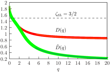
Figure 17: (color online) Generalized dimensions $D(q)$ and $\tilde{D}(q)$ at criticality $T=T_{c,\kappa}$. The dashed line is $D_{T>T_{c}}=3/2$. Solid lines are monomial fits for large q, see text.

For Anderson transitions, the finite-size scaling of the $Y_{q}$ at criticality does involve the multifractal spectrum but only one correlation length exponent $\nu$ Monthus2006a ; Huckestein1995 ,

$$\overline{Y_{q}}=L^{-\tilde{\tau}(q)}f((T_{c}-T)L^{1/\nu}).$$ (58)

Thus, it allows for a completely independent validation (cf. Fig. 18) of the critical temperature and the correlation length exponent, yielding a more exact value $T_{c}\approx 1.44$ compatible with our result from sections VII.2 and VII.4 and unambiguously a value $1/\nu\approx 0.5$ for the correlation length exponent.

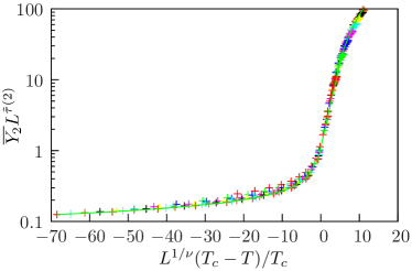
Figure 18: Finite size scaling $\overline{Y_{2}}L^{\tilde{\tau}(2)}((T_{c}-T)/T_{c}\cdot L^{1/\nu})$ giving $\nu=2$ and $T_{c}=1.41429$ for lengths $L=20,30,\ldots,100$, the points for $L=100$ are interconnected by a line as a visual guidance. This does not work for the alternatively proposed value $\nu=4$. For $T<T_{c}$, $\overline{Y_{2}}$ remains finite for large $L$ and, therefore, the finite size scaling observable diverges as $L^{\tilde{\tau}(2)}$.

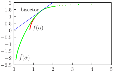
Figure 19: (color online) The singularity spectrum $f(\alpha)$, see eq. (60). For a better comparison with the expectations the plot also shows lines corresponding to $f(\alpha)=D(2)=2$, $f(\alpha)=D(1)$ and $f(\alpha)=\alpha$, see text. The bisector and $f(\alpha)$ touch at an $\alpha$ that is slightly smaller than $\alpha=1.5$. We consider this to be wrong, but it is consistent with the determined generalized dimensions, see also Fig. 20.

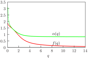
Figure 20: (color online) The directly measurable $\alpha(q)$ (green) and $f(q)$ (red) from which Fig. 19 was created. The contact point is at $\alpha=f(\alpha)\approx 1.4$

An equivalent description of the multifractal nature is related to the Legendre transform $f(\alpha)$ of $\tau(q)$ given by

$$q =f^{\prime}(\alpha)$$ (59a)

$$\tau(q) =\alpha q-f(\alpha).$$ (59b)

The function $f(\alpha)$ is called the singularity spectrum, because it gives the number $N(\alpha)\sim L^{f(\alpha)}$ of points $z$, where the weight $w(z)$ has a singularity $w\sim L^{-\alpha}$. A Legendre transform of the measured $\tau(q)$ and $\tilde{\tau}(q)$ would require an analytical continuation and, thus, be very error-prone. Fortunately, it is possible to directly measure $\alpha(q)$ and $f(q)$ Chhabra1989 and, thus, the singularity spectrum $f(\alpha)$ parametrically:

$$f(q) =-\lim_{L\rightarrow\infty}\overline{\sum_{i}\mu(q,z_{i})\ln{\mu(q,z_{i})}}/\ln{L}$$ (60a)

$$\alpha(q) =-\lim_{L\rightarrow\infty}\overline{\sum_{i}\mu(q,z_{i})\ln{w(z_{i})}}/\ln{L}$$ (60b)

with

$$\mu(q,z_{i}) \equiv w^{q}(z_{i})/(\sum_{j}w^{q}(z_{j})).$$ (60c)

This method of computing $$f(\alpha) \tau(q)$$ gives the Legendre transform of , because eq. (59) implies (omitting the limits)

$$\tau(q) =\alpha(q)q-f(q)$$

$$=-\overline{\ln{\sum_{i}w^{q}(z_{i})}}/\ln{L}$$ (60d)

$$=-\overline{\ln{Y_{q}(L)}}/\ln{L}$$

in agreement with eq. (56b), and, therefore, $f(\alpha)$ corresponds to typical values of $Y_{q}$. Note that $\alpha(q)=\tau^{\prime}(q)$ is fulfilled by construction. This is the common definition of the (multifractal) singularity spectrum that is also applicable for non-disordered systems.

Here, disorder is relevant and we need to capture not only the typical, but also the (differing, cf. Fig. 17) average behavior. Analogously to eq. (60) we derive the following computation of the Legendre transform $\tilde{f}(\tilde{\alpha})$ of $\tilde{\tau}(q)$ (we distinguish between $\alpha$ and $\tilde{\alpha}$ to avoid ambiguities as both are directly measured). We use eq. (56) and the inverse transform of (59)

$$\tilde{\tau}(q) =-\ln{\overline{\sum_{i}w^{q}(z_{i})}}/\ln{L}$$ (61a)

$$\tilde{\alpha}(q) =\tilde{\tau}^{\prime}(q)$$

$$=-\overline{\sum_{i}w^{q}(z_{i})\ln{w(z_{i})}}/(\ln{L}\cdot\overline{\sum_{i}w^{q}(z_{i})})$$ (61b)

$$\tilde{f}(\tilde{\alpha}) =\tilde{\alpha}q-\tilde{\tau}(q)$$ (61c)

$$=-\overline{\sum_{i}w^{q}(z_{i})(\ln{w^{q}(z_{i})}/\overline{\sum_{j}w^{q}(z_{j})}-1)}/\ln{L}.$$

The spectrum $f(\alpha)$ is shown in Fig. 19. Its shape matches the expectations that origin from general properties and the known results for the DL Monthus2007 and is consistent with the results for the Legendre transform $\tau(q)$. Our results show that $f(\alpha)$ is a monotonic function starting at a finite $\alpha_{\text{min}}=D_{\text{min}}(q)\approx 0.8$ which is close to the DL value $\alpha_{\tau}^{min}\approx 0.77$ and ending at $\alpha_{max}=\infty$, which corresponds to the infinitely large values $\tau(q)$ for $q<0$. The maximum value of $f(\alpha)$ is $f(\alpha\rightarrow\infty)\rightarrow D(0)$ and it touches the bisector $f=\alpha$ around $\alpha=D(1)\approx 1.4$, thus confirming the previously found deviation $D(1)\neq 3/2$. We see no indication that $f(\alpha)$ becomes negative somewhere, which would describe rare events (number decreases exponentially in $L$), but this is to be expected as $f(\alpha)$ contains the typical behavior and should not become negativeMonthus2007 . The average behavior that leads to $\tilde{f}(\tilde{\alpha})$ does include rare events and does not seem to have a finite $\alpha_{min}$, implying $\tilde{D}(\infty)=0$. We back this by noting that the we can achieve a good fit of the data for $\tau(q)$ and $\tilde{\tau}(q)$ at large q (we used $5<q<20$) with an monomial Ansatz $f(q)=aq^{b}$. For an approximate analysis we round $b$ to one decimal giving

$$\tau(q\gg 1) \approx aq$$ (62)

$$\tilde{\tau}(q\gg 1) \approx\tilde{a}q^{2/5}$$ (63)

with some constants $a,\tilde{a}$. We apply the Legendre transform and get for $q\gg 1$

$$\alpha(q) \approx a\approx 0.81 \qquad f(\alpha) \approx 0$$

$$\tilde{\alpha}(q) \sim q^{-3/5}\rightarrow 0 \qquad\tilde{f}(\tilde{\alpha}) \sim-\tilde{\alpha}^{-2/3}\rightarrow-\infty$$

In summary, we see a (Anderson transition-like) scenario in the multifractal analysis of the localization transition of a SDL in 1+1 dimensions which is very similar to the findings in Ref. Monthus2007 for a DL in 1+3 dimensions despite obvious differences due to the different geometry. In particular, the multifractal structure of the statistical weights differs between typical and average values both for DLs and SDLs. This becomes apparent in the generalized dimensions $D(q),\tilde{D}(q)$, which differ for $q\gtrapprox 1.5$. We also find a matching critical correlation length exponent $\nu$. Additionally, we showed that the average behavior is significantly influenced by rare events, leading to negative values in $\tilde{f}$, the Legendre transform of $\tilde{D}(q)$. The significance of rare (extreme) events at criticality is in accordance with our findings for the energy distribution.

VIII Conclusion

We studied stiff directed lines (SDLs) in 1+d dimensions subject to quenched short-range random potential analytically and numerically. Using Flory-type scaling arguments and a replica calculation we show that, in dimensions $d>2/3$, a localization transition exists from a high temperature phase, where the system is essentially annealed, to a disorder dominated low temperature phase. The low temperature phase is characterized by large free energy fluctuations with an exponent $\omega>0$ and a roughness exponent $\zeta$, which slightly exceeds the thermal value $\zeta_{th}=3/2$ for a SDL. Flory arguments suggest $\zeta=7/(4+d)$ for a SDL. Both exponents are related by $\omega=2\zeta-3$.

We find a reduction of the persistence length of a stiff directed line by disorder. In the low temperature phase, the persistence length is disorder-induced and temperature-independent.

We also performed variational replica functional renormalization group (FRG) calculations. The replica approach gives no conclusive results on the exponents for $d>2/3$ but supports the existence of a localization transition. The FRG calculation is performed for D+d dimensional manifolds governed by bending energies with the SDL corresponding to D=1 and employs an expansion in $\epsilon=8-D$ dimensions. For a SDL in 1+d dimensions, the FRG result suggests the existence of an upper critical dimension $d_{u}<1$, which we can rule out by numerical calculations.

For the SDL in 1+1 dimensions we performed extensive numerical transfer matrix calculations and find the existence of a localization transition and an exponent $\omega\approx 0.18$ in the low temperature disorder dominated phase. The value for $\omega$ is close to the established value $\omega\approx 0.186$ for directed lines (DLs) under tension in 1+3 dimensions. Moreover, the rescaled free energy distributions are identical. Both points suggest that the nature of the low-temperature phase is very similar, if not identical.

The multifractal analysis reveals a very similar structure of the statistical weights at the critical temperature for DLs in 1+3 dimensions and SDLs in 1+1 dimensions. It also allows for a determination of the correlation length exponent $\nu$, for which we find, again in accordance with the findings for a DL in 1+3 dimensions, $\nu=2$. Additionally, we find evidence for the relevance of rare events at criticality.

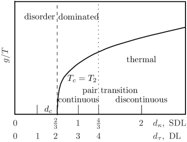
Figure 21: Schematic summary of our results supporting a relation between DLs in 1+3d and SDLs in 1+d dimensions and the importance of replica pair interactions for the localization transition in a random potential.

This strongly supports a relation between DLs in 1+3d and SDLs in 1+d dimensions, which is based on identical return exponents $\chi$ for two replicas to meet. The validity of a relation based on properties of a single replica pair suggests that the critical properties of DLs in a short-range random potential are governed by replica pair interactions. The mapping can make DL transitions in high dimensions computationally accessible, which we demonstrated in showing that the two-replica overlap provides a valid order parameter across the localization transition of SDLs in 1+1 dimensions. Furthermore, the importance of pair interactions suggests that the critical temperature for DLs in random potentials is indeed identical to the temperature below which the ratio of the second moment of the partition function and the square of its first moment diverges, which implies that the localization transition temperature $T_{c}$ in a random potential equals the replica pair transition temperature $T_{2}$ for replica pair binding. The equality $T_{2}=T_{c}$ has been originally put forward and verified numerically for DLs in 1+3 dimensions Monthus2006a ; Monthus2007 . Using the numerical transfer matrix approach we could verify this conjecture also for SDLs in 1+1 dimensions. Our findings are summarized schematically in Figs. 2 and 21.

The binding transition of DL pairs becomes discontinuous for $d>4$ and, analogously, the binding of SDL pairs for $d>4/3$ Kierfeld2003 ; Kierfeld2005 . Because DLs in random potentials are equivalent to the KPZ equation Kardar1986 , the validated relation to the SDL suggests that the roughening transition of the KPZ problem could acquire similar discontinuous features for $d>4$ dimensions. Thus, $d=4$ would remain a special dimension, although it is not the upper critical dimension Marinari2002 .

IX Acknowledgments

We acknowledge financial support by the Deutsche Forschungsgemeinschaft (KI 662/2-1).

References

- (1) T. Halpin-Healy and Y. Zhang, Phys. Rep. 254, 215 (1995).
- (2) M. Kardar, G. Parisi, and Y.C. Zhang, Phys. Rev. Lett. 56, 889 (1986).
- (3) J. Krug, Adv. Phys. 46, 139 (1997).
- (4) G. Blatter, M.V. Feigelman, V.B. Geshkenbein, A.I. Larkin, and V.M. Vinokur, Rev. Mod. Phys. 66, 1125 (1994).
- (5) T. Nattermann and S. Scheidl, Adv. Phys. 49, 607 (2000).
- (6) P. J. Yunker, M. A. Lohr, T. Still, A. Borodin, D. J. Durian, and A. G. Yodh, Phys. Rev. Lett. 110, 035501 (2013).
- (7) J.Z. Imbrie and T. Spencer, J. Stat. Phys. 52, 609 (1988).
- (8) B. Derrida and O. Golinelli, Phys. Rev. A 41, 4160 (1990).
- (9) J.M. Kim, A.J. Bray, and M.A. Moore, Phys. Rev. A 44, R4782 (1991).
- (10) J.M. Kim, M.A. Moore, and A.J. Bray, Phys. Rev. A 44, 2345 (1991).
- (11) C. Monthus and T. Garel, Eur. Phys. J. B 53, 39 (2006).
- (12) C. Monthus and T. Garel, Phys. Rev. E 74, 011101 (2006).
- (13) C. Monthus and T. Garel, Phys. Rev. E 74, 051109 (2006).
- (14) C. Monthus and T. Garel, Phys. Rev. E 75, 051122 (2007).
- (15) C. Monthus and T. Garel, J. Stat. Mech.: Theory Exp., P03011 (2007).
- (16) C. Monthus and T. Garel, Random polymers and delocalization transitions, Proceedings of “Inhomogeneous Random Systems”, IHP, Paris , Jan. 2006, Markov Processes Relat. Fields, 13, 731 (2007).
- (17) C. Monthus and T. Garel, J. Stat. Mech.: Theory Exp., P01008 (2008).
- (18) M. Schwartz, E. Perlsman, Phys. Rev. E 85, 050103(R) (2012).
- (19) M. Mezard, J. Phys. France 51, 1831 (1990).
- (20) S. Mukherji, Phys. Rev. E 50, R2407 (1994).
- (21) F. Comets, T. Shiga and N. Yoshida, Bernoulli 9, 705 (2003).
- (22) A. Pagnani and G. Parisi, Phys. Rev. E 87, 010102(R) (2013).
- (23) A. Dua and T. Vilgis, J. Chem. Phys. 121, 5505 (2004).
- (24) A. Barabasi and H.E. Stanley, Fractal Concepts in Surface Growth (Cambridge University Press, Cambridge, 1995).
- (25) S. Das Sarma, S.V. Ghaisas and J.M. Kim, Phys. Rev. E 49, 122 (1994).
- (26) Z. Rácz and M. Plischke, Phys. Rev. E 50, 3530 (1994).
- (27) R. Bundschuh, M. Lässig, and R. Lipowsky, Eur. Phys. J. E 3, 295 (2000).
- (28) J. Kierfeld and R. Lipowsky, J. Phys. A 38, L155 (2005).
- (29) H-H. Boltz and J. Kierfeld, Phys. Rev. E. 86, 060102(R) (2012).
- (30) R.A. Harris and J.E. Hearst, J. Chem. Phys. 44, 2595 (1966).
- (31) O. Kratky and G. Porod, Recl. Trav. Chim. Pays-Bas 68, 1106 (1949).
- (32) H. Kleinert, Path Integrals in Quantum Mechanics, Statistics, Polymer Physics, and Financial Markets (World Scientific, Singapore, 2006).
- (33) P. Gutjahr, R. Lipowsky, and J. Kierfeld, Europhys. Lett. 76, 994 (2006).
- (34) G. Gompper and T.W. Burkhardt, Phys. Rev. A 40, 6124 (1989).
- (35) M.E. Fisher, J. Stat. Phys. 34, 667 (1984).
- (36) R. Bundschuh and M. Lässig, Phys. Rev. E 54, 304 (1996).
- (37) S. Mukherji, S.M. Bhattacharjee, Phys. Rev. B 53, R6002 (1996).
- (38) D. S. Fisher and D. A. Huse, Phys. Rev. B 43, 10728 (1991).
- (39) A. Engel, Nucl. Phys. B 410, 617 (1993).
- (40) P. Le Doussal, K. J. Wiese and P. Chauve, Phys. Rev. E 69, 026112 (2004).
- (41) V. Dotsenko, Introduction to the Replica Theory of Disordered Statistical Systems (Cambridge University Press, Cambridge, 2001).
- (42) M. Mezard, G. Parisi, J. Physique I 1, 809 (1991).
- (43) G. Parisi, J. Phys. A 13, 1887 (1980).
- (44) M. Kardar, Nucl. Phys. B 290, 582 (1987).
- (45) D.S. Fisher, Phys. Rev. Lett. 56, 1964 (1986).
- (46) L. Balents, D.S. Fisher, Phys. Rev. B 48, 5949 (1993).
- (47) P. Chauve, P. Le Doussal and K. J. Wiese, Phys. Rev. Lett. 86, 1785 (2001).
- (48) P. Le Doussal, K. J. Wiese and P. Chauve, Phys. Rev. B 66, 174201 (2002).
- (49) P. Le Doussal and K. J. Wiese, Phys. Rev. E 72, 035101(R) (2005).
- (50) X. Wang, S. Havlin, and M. Schwartz, J. Phys. Chem. B 104, 3875 (2000).
- (51) T. Ala-Nissila, T. Hjelt, J.M. Kosterlitz, and O. Venäläinen, J. Stat. Phys. 72, 207 (1993).
- (52) E. Marinari, A. Pagnani, and G. Parisi, J. Phys. A: Math. Gen. 33, 8181 (2000).
- (53) G. Marsaglia and W. W. Tsang, J. Stat. Soft. 5 (2000).
- (54) C.A. Doty, J.M. Kosterlitz, Phys. Rev. Lett. 69, 1979 (1992).
- (55) T. Giamarchi and P. Le Doussal, Phys. Rev. B 52, 1242 (1995).
- (56) B. Derrida and H. Flyvbjerg, J. Phys. A: Math. Gen. 20, 5273 (1987).
- (57) V. S. Dotsenko, Physics - Uspekhi 54, 259 (2011).
- (58) I.V. Kolokolov and S.E. Korshunov, Phys. Rev. B 75, 140201 (2007).
- (59) I.V. Kolokolov and S.E. Korshunov, Phys. Rev. B 78, 024206 (2008).
- (60) J. Krug and P. Meakin, J. Phys. A: Math. Gen. 23, L987 (1990).
- (61) E. J. Gumbel, 1954. Statistical theory of extreme values and some practical applications Applied Mathematics Series – 33 (National Bureau of Standards, Washington, 1954).
- (62) M. Abramowitz and I.A. Stegun, Handbook of Mathematical Functions Applied Mathematics Series – 55. (National Bureau of Standards, Washington, 1972).
- (63) J. Kierfeld and R. Lipowsky, Europhys. Lett. 62, 285 (2003).
- (64) M. H. Jensen, L. P. Kadanoff and I. Procaccia, Phys. Rev. A 36, 1409 (1987)
- (65) T. Tél, Z. Naturforsch. 43a, 1154 (1988).
- (66) B. Huckestein, Rev. Mod. Phys. 67, 357 (1995).
- (67) A. Chhabra and R. V. Jensen, Phys. Rev. Lett. 62, 1327 (1989).
- (68) E. Marinari, A. Pagnani, G. Parisi and Z. Rácz, Phys. Rev. E 65, 026136 (2002).