Topological entanglement entropy in bilayer quantum Hall systems

Abstract

We calculate the topological entanglement entropy in bilayer quantum Hall systems, dividing the set of quantum numbers into four parts. This topological entanglement entropy allows us to draw a phase diagram in the parameter space of layer separation and tunneling amplitude. We perform the finite size scaling analysis of the topological entanglement entropy in order to see the quantum phase transition clearly.

I Introduction

None of local order parameters in some cases can distinguish the types of quantum order, because quantum nature itself is nonlocal. To overcome this difficult situation, Kitaev and Preskill Kitaev have introduced the topological entanglement entropy, which is obtained by the well-designed partition and the clever linear combination of the corresponding entanglement entropies. It is of interest to look for an explicit microscopic model that realizes quantum order characterized by the topological entanglement entropy. The purpose of this paper is to present the microscopic model related to the topological entanglement entropy.

A system with a mass gap in two spatial dimensions can exhibit topological order Wen . A mass gap is the key ingredient for the incompressible quantum Hall state Laughlin . The quasiparticle excitations in the quantum Hall system obey fractional statistics Arovas . Furthermore, Haldane Haldane showed that, in the quantum Hall system, the ground-state degeneracy depends on whether the geometry is either sphere or torus. These features of mass gap, fractional statistics, and dependence of degeneracy are all topological properties. Hence it is natural to consider the topological entanglement entropy in the quantum Hall system.

For applications of the topological entanglement entropy in relation with quantum phase transitions, we consider bilayer quantum Hall systems, where it is simpler to introduce controllable parameters into the Hamiltonian of the system. In bilayer quantum Hall systems, two parameters to be controlled are the layer separation $d$ and the inter-layer tunneling amplitude $t$. The experimental strong evidence for the quantum phase transition of bilayer systems was a strong enhancement in the zero-bias inter-layer tunneling conductance for a small $d$ system at total Landau level filling factor $\nu=1$ Spielman . Theoretically, if $d$ goes to $\infty$ for fixed $\nu=1$, the bilayer system becomes a set of two single layer systems for $\nu=\frac{1}{2}$. For a large $d$ system, the ground state would be compressible, which is not a quantum Hall state. It is clear that phase transition takes place at the critical value $d_{c}$ which is met while $d$ changes from $0$ to $\infty$. The main concern is now to draw the phase diagram of the system in the parameter space of $d$ and $t$.

Pseudospin notation for the layer degree of freedom is used to find the phase diagram, by calculating the pseudospin magnetization Schliemann . However this pseudospin magnetization approach is not conclusive because calculations of varying $d$ for fixed $t$ give different results from those of varying $t$ for fixed $d$. Since the pseudospin is a local order parameter, the approach of the pseudospin magnetization may not provide perfect explanation for the nature of quantum phase transitions in bilayer quantum Hall systems.

In this paper, we focus on the topological entanglement entropy, which is the most natural order parameter to study phase transition in bilayer quantum Hall systems. Using exact diagonalization, we numerically evaluate the topological entanglement entropy in finite size systems. We analyze the behavior of the topological entanglement entropy as we vary $d$ for fixed $t$. We also carry out the analysis of finite size scaling. We will show that the topological entanglement entropy provides a different phase boundary from that of the pseudospin magnetization in bilayer quantum Hall systems. This difference is controversial. More detailed experimental measurements are required to resolve the issue of topological entanglement entropy as an order parameter for bilayer quantum Hall systems.

II Hamiltonian

We start with presenting the bilayer quantum Hall system in terms of the second quantized form of the Hamiltonian in a torus geometry within the lowest Landau level approximation. It is known that the Landau level degeneracy $N$ is determined by the magnetic field strength $B$ and the square torus area $L^{2}$ as $L^{2}=2\pi Nl_{B}^{2}$ where $l_{B}=\sqrt{\hbar c/eB}$ is the magnetic length. It is convenient to measure all distances in the unit of $l_{B}$, and energies in the unit of $e^{2}/\epsilon l_{B}$, where $\epsilon$ is a dielectric constant.

The two-body interaction between electrons is described by the periodic Coulomb interaction $U(\vec{x}_{i}-\vec{x}_{j})$, which is written in terms of position variables $\vec{x}$ and momentum variables $\vec{k}$ by using the Fourier transformation:

$$U(\vec{x}_{i}-\vec{x}_{j})=\frac{e^{2}}{\epsilon|\vec{x}_{i}-\vec{x}_{j}|}=\lim_{\mu\rightarrow 0}\frac{e^{2}}{\epsilon(2\pi)^{3}}\int d^{3}k\frac{4\pi}{k^{2}+\mu^{2}}\exp[i\vec{k}\cdot(\vec{x}_{i}-\vec{x}_{j})],$$

where $\mu$ is introduced in order to take into account the infrared divergence. If two electrons are on the same (different) layer, intra (inter) layer, the third component of $(\vec{x}_{i}-\vec{x}_{j})$ is $0$ ($d$). In the torus geometry of the finite size $L^{2}$, the first and second components $k_{1}$ and $k_{2}$ out of $\vec{k}$ turn to the discrete integers $n_{1}$ and $n_{2}$, while $k_{3}$ is kept as continuous. Then $U(\vec{x}_{i}-\vec{x}_{j})$ between inter-layer electrons is written as

$$U(\vec{x}_{i}-\vec{x}_{j})=\frac{e^{2}}{\epsilon 2\pi^{2}}\left(\frac{2\pi}{L}\right)^{2}\{\lim_{\mu\rightarrow 0}\int_{-\infty}^{\infty}dk_{3}\frac{\exp(ik_{3}d)}{k_{3}^{2}+\mu^{2}}$$

$$+\sum_{(n_{1},n_{2})\neq(0,0)}\int_{-\infty}^{\infty}dk_{3}\frac{\exp[i\frac{2\pi}{L}\vec{n}\cdot(\vec{x}_{i}-\vec{x}_{j})+ik_{3}d]}{(\frac{2\pi}{L}n_{1})^{2}+(\frac{2\pi}{L}n_{2})^{2}+k^{2}_{3}}\},$$

where the first term is extracted as the infrared divergence part for the case of $n_{1}=n_{2}=0$. Integrating out $k_{3}$, we obtain

$$U(\vec{x}_{i}-\vec{x}_{j})=\lim_{\mu\rightarrow 0}\frac{e^{2}}{\epsilon L}2\pi\frac{\exp(-\mu d)}{L\mu}$$

$$+\frac{e^{2}}{\epsilon L}\sum\frac{\exp[-\sqrt{n_{1}^{2}+n_{2}^{2}}\frac{2\pi}{L}d]}{\sqrt{n_{1}^{2}+n_{2}^{2}}}\exp[i\frac{2\pi}{L}\vec{n}\cdot(\vec{x}_{i}-\vec{x}_{j})].$$

Expanding $\exp(-\mu d)$ into the Taylor series with respect to $\mu$, we rewrite the first term of $U(\vec{x}_{i}-\vec{x}_{j})$ as follows:

$$\frac{e^{2}}{\epsilon L}2\pi\frac{\exp(-\mu d)}{L\mu}=\frac{e^{2}}{\epsilon l_{B}}\frac{1}{Nl_{B}\mu}-\frac{e^{2}}{\epsilon l_{B}}\frac{d}{Nl_{B}}+\mathcal{O}(\mu).$$

The infinite first term explains the infrared divergence, and it should be canceled by uniform positive background charge Shibata . The finite second term which depends on $d$ contributes to a static charging-energy Nomura .

The Fourier transformation and handling the infrared divergence make it straightforward to derive the second quantized Hamiltonian by using the single particle wave-function. For the lowest Landau level in the torus geometry, the $j$-th single particle wave-function $\psi_{j}(x,y)$ Cristofano is given by

$$\psi_{j}(x,y)=(\frac{1}{L\sqrt{\pi}l_{B}})^{1/2}\exp(-\frac{y^{2}}{2l_{B}^{2}})$$

$$\times\sum_{k=-\infty}^{\infty}\exp[-\pi N(k+\frac{j}{N})^{2}+i2\pi N(k+\frac{j}{N})(\frac{x+iy}{L})].$$

The Hamiltonian $H$ for the bilayer quantum Hall system is the sum of the Coulomb interaction term $H_{i}$ and the single particle inter-layer tunneling term $H_{t}$ such as

$$H=H_{i}+H_{t}.$$ (1)

Based on the above wave functions $\psi_{j}(x,y)$ and the periodic Coulomb interaction $U(\vec{x}_{i}-\vec{x}_{j})$, we obtain the second quantized form of $H_{i}$. The Hamiltonian is expressed in terms of creation and annihilation operators $c_{j\sigma}^{\dagger}$ and $c_{j\sigma}$, where pseudospin $\sigma=\uparrow$ or $\downarrow$ is used to describe different layers. We get

$$H_{i}=H_{\uparrow}+H_{\downarrow}+H_{\uparrow\downarrow}-\frac{e^{2}}{\epsilon l_{B}}\frac{d}{l_{B}}\frac{N_{\uparrow}N_{\downarrow}}{N},$$ (2)

where $H_{\uparrow}$ ($H_{\downarrow}$) presents the interaction between electrons in up (down) layer, $H_{\uparrow\downarrow}$ is the inter-layer Hamiltonian, and $N_{\uparrow}$($N_{\downarrow}$) in charging-energy term is the number of electrons in up (down) layer. The value of product $N_{\uparrow}N_{\downarrow}$ is maximized at $N_{\uparrow}=N_{\downarrow}=N/2$ with the constraint of $N_{\uparrow}+N_{\downarrow}=N$. Without the last term, all electrons stay in a single layer according to Hund’s rule for a small $d$ as shown in Table 1.

Following the procedure given by Yoshioka-Halperin-Lee Yoshioka , we find

$$H_{\sigma} = \frac{1}{2}\sum_{a,b=0}^{N-1}V(a,b;0)\sum_{k=0}^{N-1}c_{k+a\sigma}^{\dagger}c_{k+b\sigma}^{\dagger}c_{k+a+b\sigma}c_{k\sigma},$$

$$H_{\uparrow\downarrow} = \sum_{\sigma\not=\sigma^{\prime}}\frac{1}{2}\sum_{a,b}V(a,b;d)\sum_{k}c_{k+a\sigma}^{\dagger}c_{k+b\sigma^{\prime}}^{\dagger}c_{k+a+b\sigma^{\prime}}c_{k\sigma}.$$

Here the orbital index $j$ in $c_{j\sigma}^{\dagger}$ should satisfy the periodic condition such that $c^{\dagger}_{j+N~{}\sigma}=c^{\dagger}_{j~{}\sigma}$. The coefficients $V$ in the Hamiltonian are given by

$$V(a,b;d)=\sum_{m,l\in\mbox{Z}}g(Nm+a,l)\exp(-\frac{\pi}{N}\{l^{2}+(Nm+a)^{2}\})\cos(\frac{2\pi}{N}lb),$$

$$g(i,j)=\frac{e^{2}}{\epsilon l_{B}}\frac{1}{N}\frac{\exp[-\sqrt{\frac{2\pi}{N}(i^{2}+j^{2})}\frac{d}{l_{B}}]}{\sqrt{\frac{2\pi}{N}(i^{2}+j^{2})}},$$

where the case of $g(0,0)$ is excluded since the infrared divergence was already handled Chung1 .

The single particle tunneling term $H_{t}$ is written as

$$H_{t}=-\frac{e^{2}}{\epsilon l_{B}}t\frac{1}{2}\sum_{j}\sum_{\sigma\sigma^{\prime}}c^{\dagger}_{j\sigma}s^{\sigma\sigma^{\prime}}_{x}c_{j\sigma^{\prime}},$$ (3)

where $s^{\sigma\sigma^{\prime}}_{x}$ is the pseudospin Pauli matrix and $t$ measures the inter-layer tunneling amplitude.

After we set the Hamiltonian, we perform exact diagonalization to find the ground state of a small system. Doing consistency checks, we show explicit values of the ground state energy for the system of $N=8$ in Table 1.

When the layer separation vanishes ($d=0$) and no tunneling is allowed ($t=0$), the Hamiltonian has pseudospin SU(2) rotational symmetry. It means $[H_{i},\vec{S}]=0$, where $\vec{S}$ is the total pseudospin operator Nomura . Then the ground state should be also the eigenstate of the $\vec{S}^{2}$ and $S_{z}$. In Table 1, the same values of ground state energy for $d=0$ and $t=0$ system reflect SU(2) pseudospin symmetry.

The eigenvalues of $S_{z}$ are given by $(N_{\uparrow}-N_{\downarrow})/2$. We find that our charging-energy term is related to $S_{z}$ MacDonald as

$$-\frac{e^{2}}{\epsilon l_{B}}\frac{d}{l_{B}}\frac{N_{\uparrow}N_{\downarrow}}{N}=\frac{e^{2}}{\epsilon l_{B}}\frac{d}{l_{B}}\frac{-(N_{\uparrow}+N_{\downarrow})^{2}+(N_{\uparrow}-N_{\downarrow})^{2}}{4N}=-\frac{e^{2}}{\epsilon l_{B}}\frac{d}{l_{B}}\frac{1}{4}N+\frac{e^{2}}{\epsilon l_{B}}\frac{d}{l_{B}}\frac{1}{N}S_{z}^{2},$$

where the ground state prefers $S_{z}=0$.

$(N_{\uparrow},N_{\downarrow})$	(4,4)	(5,3)	(6,2)	(7,1)	(8,0)
$H_{\uparrow}+H_{\downarrow}+H_{\uparrow\downarrow}$	$-2.864848$	$-2.864848$	$-2.864848$	$-2.864848$	$-2.864848$
$-\frac{e^{2}}{\epsilon l_{B}}\frac{d}{l_{B}}\frac{N_{\uparrow}N_{\downarrow}}{N}$	0	0	0	0	0
$H_{i}$ at $d/l_{B}=0.0$	$-2.864848$	$-2.864848$	$-2.864848$	$-2.864848$	$-2.864848$
$H_{\uparrow}+H_{\downarrow}+H_{\uparrow\downarrow}$	$-2.678141$	$-2.689105$	$-2.724817$	$-2.783162$	$-2.864848$
$-\frac{e^{2}}{\epsilon l_{B}}\frac{d}{l_{B}}\frac{N_{\uparrow}N_{\downarrow}}{N}$	$-0.2$	$-0.1875$	$-0.15$	$-0.0875$	0
$H_{i}$ at $d/l_{B}=0.1$	$-2.878141$	$-2.876605$	$-2.874817$	$-2.870662$	$-2.864848$

Table 1: Consistency checks for ground state energy. For $t=0.0$, we can divide the Hilbert space according to $N_{\uparrow}$ and $N_{\downarrow}$. We present the ground state energy in each sector for the case of $t=0.0$ and $N=8$, comparing $d/l_{B}=0.0$ to $d/l_{B}=0.1$. Without the term of charging-energy, the sector of $(N_{\uparrow},N_{\downarrow})=(8,0)$ contains the true ground state at $d/l_{B}=0.1$ like Hund’s rule.

III Topological Entanglement Entropy

In order to find the entanglement entropy which is a nonlocal quantity Berrada , we first conduct bipartition. We can arbitrarily divide the space into two parts, $A$ and $B$. Then, we calculate the von Neumann entropy $S_{A}$ as follows:

$$S_{A}=-\mbox{Tr}\rho_{A}\log_{2}\rho_{A},~{}~{}~{}~{}~{}\rho_{A}=\mbox{Tr}_{B}|\Psi_{0}\rangle\langle\Psi_{0}|.$$ (4)

Here, the ground state $|\Psi_{0}\rangle$ with $M$ electrons is spanned by the basis $\{|i\rangle\}$:

$$|\Psi_{0}\rangle = \sum_{i}a_{i}|i\rangle$$ (5)

$$= \sum_{i}a_{i}c^{\dagger}_{i_{1}}c^{\dagger}_{i_{2}}\cdots c^{\dagger}_{i_{M}}|0\rangle$$

$$= \sum_{i}a_{i}(-1)^{P}c^{\dagger}_{j_{1}}\cdots c^{\dagger}_{j_{M_{A}}}c^{\dagger}_{k_{1}}\cdots c^{\dagger}_{k_{M_{B}}}|0\rangle,$$

where the creation operators should be reordered such that $j_{1}<\cdots<j_{M_{A}}$ in the subsystem $A$, $k_{1}<\cdots<k_{M_{B}}$ in $B$, and $M_{A}+M_{B}=M$. The sign $(-1)^{P}$ should be taken care of during the reordering step. In some systems, this entropy $S_{A}$ indicates critical points of quantum phase transitions Chung2 . However, this single entanglement entropy $S_{A}$ does not always indicate critical points. According to our calculations, in bilayer quantum Hall systems, the single entanglement entropy $S_{A}$ for bipartition of up layer $A$ and down layer $B$ can not indicate critical points. Thus, it is necessary to introduce slightly more complicated entropies in addition to $S_{A}$ to form the order parameter. It is also interest to investigate entanglement spectrum Schliemann2 .

Now let us turn our attention to the recent proposal Kitaev of the topological entanglement entropy. Our system described by the Hamiltonian of Eq. (1) looks like a one-dimensional system with a single index, because of the lowest Landau level approximation. However, our original physical space is two-dimensional and our system shows topological properties.

Since systems have the same number of quantum numbers as their spatial dimensions, our system in two spatial dimensions has two quantum numbers $(n,j)$ by ignoring spin and pseudospin, where $n$ denotes the Landau level, $n=0\cdots\infty$, and $j$ denotes the intra-Landau level, $j=0\cdots N-1$. Here the Landau level degeneracy $N$ plays the role of width in this two-dimensional quantum number space. In the lowest Landau level approximation, we restrict the quantum number space into $n=0$ space alone. Now we should find a good bipartition of the lowest Landau level, where the boundary length between $A$ and $B$ is proportional to $N$ to guarantee large subspaces $A$ and $B$. The leading term of the corresponding von Neumann entropy $S_{A}$ then can be proportional to $N$ such as $S_{A}=\alpha N-\gamma+\cdots$. The even-odd bipartition Chen in the one-dimensional spin system was considered to obtain a large entanglement entropy. We will apply this kind of partition to our bilayer quantum Hall system.

In order to study a topological property of bilayer quantum Hall systems with the Hamiltonian Eq. (1), we consider the topological entanglement entropy $S_{topo}$ Kitaev defined as

$$S_{topo}=S_{A}+S_{B}+S_{C}-S_{AB}-S_{BC}-S_{CA}+S_{ABC},$$ (6)

where it is crucial to partite the one-dimensional index system into four lattice subsystems, $A$, $B$, $C$ and $D$. Keeping in mind the requirement that all seven entropies in Eq. (6) should be proportional to $N$, we make the following partition. As shown in Fig. 1, we partite the index system of $\{j,\sigma\}$ in $c^{\dagger}_{j\sigma}$ such as $j\mod 3=0,1,2$ in up layer ($\sigma=\uparrow$) for $A$, $B$, $C$, respectively, and $D$ denotes all $j$ in down layer ($\sigma=\downarrow$). The subsystem $AB$ represents $A\cup B$, etc. Numerical results confirm that all entanglement entropies in Eq. (6) are proportional to $N$ for small $d$.

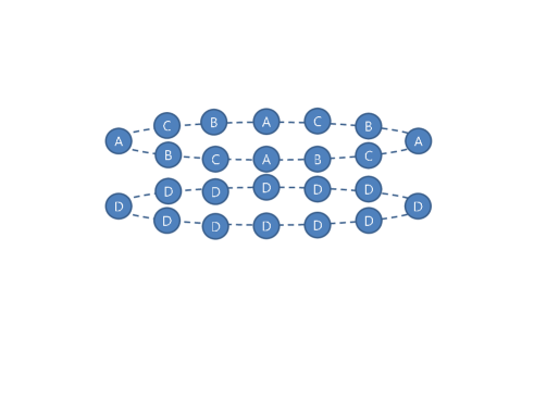
Figure 1: For $N=12$, a highly entangled partition into four regions. This type of partition is adopted during the calculations.

A slight change of topology does not effect on the value of $S_{topo}$. However, it should be emphasized that a topologically different partition provides a different entanglement entropy. For example, we can divide the index system into four regions such as $A^{\prime}$ is even in up layer, $B^{\prime}$ is odd in up layer, $C^{\prime}$ is even in down layer, and $D^{\prime}$ is odd in down layer. We find however that $S^{\prime}_{topo}$ for this type of partition does not play the role of the order parameter to explain the phase transition. In consequence, we should make an adequate choice of partition to get the proper topological entanglement entropy explaining the phase transition.

IV Numerical Works

To compute the topological entanglement entropy $S_{topo}$, we first look for the ground state $|\Psi_{0}\rangle$ of the system, by diagonalizing the Hamiltonian $H$ of Eq. (1). The main calculation is to find the coefficients $a_{i}$ of Eq. (5) as the coupling parameter $d$ changes for fixed $t$. The explicit forms of the density matrices are determined by reordering indices in Eq. (5). Then, we find the von Neumann entropies by diagonalizing the density matrices. Finally the topological entanglement entropy is obtained as the combination of the von Neumann entropies in Eq. (6).

Before we present numerical results, the number of electrons $M$ is worthy of mentioning. Since the last term of the Hamiltonian in Eq. (2) prefers equal number of electrons in up and down layers, the ground state with even number of electrons has very small electron number fluctuation in a typical finite size calculation. Since the number fluctuation is essential for phase transition, we should choose finite systems with odd number of electrons. Odd number systems can circumvent unwanted effects of charging-energy cost in finite systems because one additional electron fluctuating between two layers does not cost charging-energy.

Because of the advantage of odd number of electrons, we have computed the topological entanglement entropy $S_{topo}$ up to odd $M=13$ as a function of the layer separation $d$ for various values of the tunneling amplitude $t$, which is plotted in Fig. 2. The shape of the topological entanglement entropy in bilayer quantum Hall systems is similar to the spontaneous magnetization in the Ising model Landau .

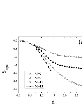
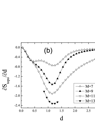
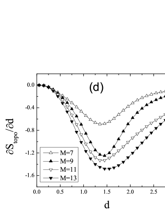
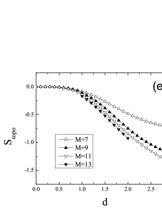
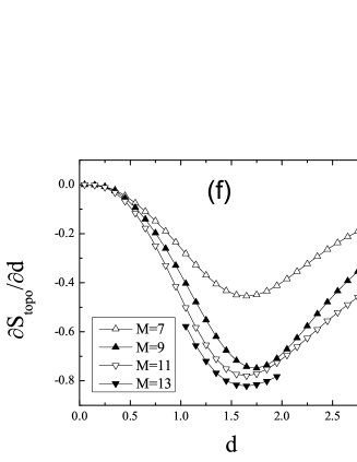
Figure 2: The entropy $S_{topo}$ versus the layer separation $d$, and the derivative of the entropy $\partial S_{topo}/\partial d$ versus $d$ for three fixed values of $t$: (a) and (b) $t=0.01$, (c) and (d) $t=0.05$, (e) and (f) $t=0.1$. We notice that there are the pronounced dips in $\partial S_{topo}/\partial d$ at nearly the same $d$ for each $t$.

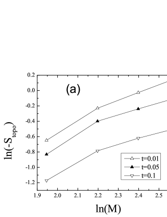
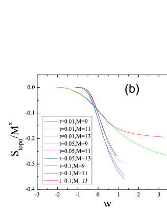
Figure 3: (Color online) (a) The logarithm of the entropy $\ln(-S_{topo})$ versus the logarithm of the number of electrons $\ln(M)$. Ignoring the data of $M=7$, we notice the linear relationship between the two values. It is easy to determine the slope which gives $x$ shown in Table 2. (b) The entropy $S_{topo}$ versus the scaled parameter $w=\epsilon M^{1/\nu}$ where $\epsilon=(d-d_{c})/d_{c}$. A good data collapse is found at $1/\nu=0.3$ for the data of $t=0.01$, at $1/\nu=0.05$ for the data of $t=0.05$, and at $1/\nu=0.01$ for the data of $t=0.1$.

In general, the phase boundary between quantum Hall state and compressible states can be obtained at the point where the topological entanglement entropy changes most and it has the maximum negative slope. Fig. 2 shows the maximum negative slopes. Specifically, the plot of $\partial S_{topo}/\partial d$ in Fig. 2(b) shows a dip at $d\simeq 1.1l_{B}$ for $t=0.01$. This may be a signature of transition from coherent to incoherent quantum phase.

We postulate the scaling function $\Theta$ to present the topological entanglement entropy $S_{topo}$ as

$$S_{topo}=M^{x}\Theta(\epsilon M^{\frac{1}{\nu}}).$$ (7)

For the purpose of making a data-collapse, we look for the scaling exponents $x$ and $1/\nu$ as a function of the tunneling amplitude $t$. In order to find the exponent $x$, we use the data of the critical point where $\epsilon\equiv(d-d_{c})/d_{c}=0$. In Fig. 3(a), we find that $S_{topo}$ is very well proportional to $M^{x}$ as far as we ignore the data of $M=7$, that is, $\ln M\simeq 1.946$. Once we have determined $d_{c}$ and $x$, the determination of $1/\nu$ gives the data-collapse. As shown in Fig. 3(b), all data of Fig. 2 are collapsed into a single line near at the scaled parameter $w\equiv\epsilon M^{\frac{1}{\nu}}=0$. The numerical results are summarized in Table 2.

$t$	$d_{c}$	$x$	$1/\nu$
$0.01$	$1.1\pm 0.04$	$0.99\pm 0.03$	$0.3\pm 0.05$
$0.05$	$1.4\pm 0.05$	$0.76\pm 0.05$	$0.05\pm 0.1$
$0.1$	$1.6\pm 0.06$	$0.68\pm 0.08$	$0.01\pm 0.1$

Table 2: Summary of numerical results. For a given t, the values of $d_{c}$, $x$, and $1/\nu$ are calculated. For $t=0.01$, the data-collapse at $1/\nu=0.3$ looks more likely a single line than at $1/\nu=0.35$, so that we roughly estimate the error. However, it is hard to distinguish the better data-collapse by changing the value of $1/\nu$ for $t=0.05$ or $t=0.1$, so that we present a bigger error.

To determine the phase boundary between coherent and incoherent states, we use the first derivative of topological entanglement entropy with respect to $d$. Note that the maximum of the first-derivative is a function of $t$. We drew the phase boundary by plotting the maxima of the first-derivatives with respect to $d$ in Fig. 4. The phase boundary has a slight increasing tendency as the tunneling amplitude increases. The phase boundary line looks concave from below instead of convex. The parabolic (convex) phase boundary was proposed by Murphy et al. Murphy . However, the parabolic phase boundary has a little discrepancy Spielman2 with the tunneling data as shown in Fig. 5. In fact, the critical value $d_{c}$ at $t=0$ determined by the tunneling data is less than the value given by the parabolic phase boundary line. Another point of the parabolic phase boundary is that there always exists an enough big tunneling amplitude $t$ that produces a quantum Hall state for any $d$. This means that the tunneling can produce a quantum Hall state without the inter-layer Coulomb interaction for infinitely separated bilayer systems. This dominant role of tunneling may be overestimated to produce a quantum Hall state. In order to explain the transport data and the tunneling data simultaneously, we modify the phase boundary line which is concave as shown in Fig. 5. The tunneling enhances coherence, but the inter-layer Coulomb interaction is more important for a quantum Hall state. The concave phase boundary may be reasonable.

It is known that the phase boundary line in Fig. 4 shifts upward for the system with finite layer thickness Shibata2 . Although we do not calculate explicitly here, finite layer thickness will be crucial when we try to adjust the critical values of $d_{c}$.

Figure 4: The phase boundary in the parameter space of $d$ and $t$. Slightly the less steep slopes are observed as $t$ increases.

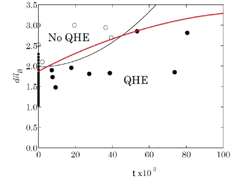
Figure 5: Data presented in Spielman’s thesis. Each circle represents a sample as measured by magneto-transport. Solid markers indicate the existence of a quantum Hall minimum, and open markers the lack thereof. The bold lines on the vertical axis represent tunneling data: the solid portion indicates the existence of a peak in tunneling and the dashed portion indicates its absence. The black line is a proposed parabolic phase boundary based on the transport data by Murphy et al. However, it is possible to propose a modified phase boundary line, which is concave from below like the red line. This red line is consistent with the tunneling data.

V Conclusion

We have considered the quantum phase transition controlled by the layer separation in bilayer quantum Hall systems. The interaction between electrons in the system is described by the Coulomb interaction in a torus geometry within the lowest Landau level approximation. The main numerical work is to compute the topological entanglement entropy by exact diagonalization. We find that the topological entanglement entropy plays the role of an order parameter to distinguish quantum phases.

In summary, we have presented the topological entanglement entropy in bilayer quantum Hall systems. We have concluded that the topological entanglement entropy is a better order parameter than the pseudospin magnetization in bilayer quantum Hall systems. The quantum order in bilayer quantum Hall systems is originated by topological properties.

- (1) A. Kitaev and J. Preskill, Phys. Rev. Lett. 96, 110404 (2006).
- (2) X.-G. Wen and Q. Niu, Phys. Rev. B41, 9377 (1990).
- (3) R. B. Laughlin, Phys. Rev. Lett. 50, 1395 (1983).
- (4) D. Arovas, J. R. Schrieffer and F. Wilczek, Phys. Rev. Lett. 53, 722 (1984).
- (5) F.D.M. Haldane, Phys. Rev. Lett. 55, 2095 (1985).
- (6) I. B. Spielman, J. P. Eisenstein, L. N. Pfeiffer and K. W. West, Phys. Rev. Lett. 84, 5808 (2000).
- (7) J. Schliemann, S. M. Girvin and A. H. MacDonald, Phys. Rev. Lett. 86, 1849 (2001).
- (8) N. Shibata and D. Yoshioka, J. Phys. Soc. Jpn., 043712 (2006).
- (9) K. Nomura and D. Yoshioka, Phys. Rev. B66, 153310 (2002).
- (10) G. Cristofano, G. Maiella, R. Musto and F. Nicodimi, Phys. Lett. B262, 88 (1991).
- (11) D. Yoshioka, B. I. Halperin and P. A. Lee, Phys. Rev. Lett. 50, 1219 (1983).
- (12) M.-H. Chung, J. Hong and J.-H. Kwon, Phys. Rev. B55, 2249 (1997).
- (13) A. H. MacDonald, P. M. Platzman and G. S. Boebinger, Phys. Rev. Lett. 65, 775 (1990).
- (14) K. Berrada, A. Mohammadzade, S. Abdel-Khalek, H. Eleuch and S. Salimi, Physica E45, 21 (2012).
- (15) M.-H. Chung and D. P. Landau, Phys. Rev. B83, 113104 (2011).
- (16) J. Schliemann, Phys. Rev. B83, 115322 (2011).
- (17) Y. Chen, P. Zanardi, Z. D. Wang and F. C. Zhang, New J. of Phys. 8, 97 (2006).
- (18) D. P. Landau, Phys. Rev. B13, 2997 (1976).
- (19) S. Q. Murphy, J. P. Eisenstein, G. S. Boebinger, L. N. Pfeiffer and K. W. West, Phys. Rev. Lett. 72, 728 (1994).
- (20) I. B. Spielman, Ph. D. Thesis, California Institute of Technology, Pasadena, 2004.
- (21) D. Yoshioka and N. Shibata, J. Phys. Soc. Jpn., 064717 (2010).