Multidimensional modeling of coronal rain dynamics

Abstract

We present the first multidimensional, magnetohydrodynamic simulations which capture the initial formation and the long-term sustainment of the enigmatic coronal rain phenomenon. We demonstrate how thermal instability can induce a spectacular display of in-situ forming blob-like condensations which then start their intimate ballet on top of initially linear force-free arcades. Our magnetic arcades host chromospheric, transition region, and coronal plasma. Following coronal rain dynamics for over 80 minutes physical time, we collect enough statistics to quantify blob widths, lengths, velocity distributions, and other characteristics which directly match with modern observational knowledge. Our virtual coronal rain displays the deformation of blobs into $V$-shaped like features, interactions of blobs due to mostly pressure-mediated levitations, and gives the first views on blobs which evaporate in situ, or get siphoned over the apex of the background arcade. Our simulations pave the way for systematic surveys of coronal rain showers in true multidimensional settings, to connect parametrized heating prescriptions with rain statistics, ultimately allowing to quantify the coronal heating input.

1 Introduction

A recurrent finding in coronal loops is the coronal rain phenomenon, seen as intensity variations signaling cool blob-like downflows along the legs of loops (Kawaguchi, 1970; Leroy, 1972; Schrijver, 2001; O’Shea et al., 2007). Coronal rain forms part of the general phenomenon of thermal instability in a plasma, that takes place whenever radiative losses locally overcome the heating input (Parker, 1953; Field, 1965), and is related to “catastrophic cooling” events (Schrijver, 2001). Meanwhile, numerical studies have significantly contributed to the understanding of these events, but typically adopted simplifying one-dimensional (1D) approximations meant to demonstrate the thermodynamic evolution along individual field lines (Goldsmith, 1971; Mok et al., 1990; Antiochos & Klimchuk, 1991; Antiochos et al., 1999; Xia et al., 2011). For coronal rain to occur in loops, the heating input is generally accepted to be concentrated at the loop footpoints. With footpoint heating, the loops rapidly get hotter and denser, due to evaporated chromospheric plasma invading the loops. The combined action of anisotropic thermal conduction and optically thin radiation causes these coronal hot loops to ultimately reach thermally unstable regimes in a timescale of hours. After that, “catastrophic cooling” sets in locally, leading to the rapid formation of condensations, as demonstrated in 1D models (Karpen et al., 2001; Müller et al., 2003, 2004, 2005; De Groof et al., 2005; Antolin et al., 2010; Xia et al., 2011). In this paper, we present the first numerical study of the coronal rain phenomenon in a 2.5-dimensional model where a magnetic arcade hosting chromospheric, transition region, and coronal plasma demonstrates a coronal rain shower lasting for over an hour. This allows us to collect statistical information that can confront recent observational insights.

From the observational side, the various stages of coronal rain formation have been analysed using TRACE, and were found to be recurring in timescales of days to weeks (Schrijver, 2001). Observations of coronal rain with Hinode/SOT have revealed a clear thread-like character in the coronal loops, and have started to provide statistical info on the number and velocities of blobs, while sizes reach down to the resolution limits (Antolin et al., 2010). High resolution instruments now reveal a scenario that coronal rain is a rather common phenomenon (Kamio et al., 2011; Antolin & Verwichte, 2011; Antolin & Rouppe van der Voort, 2012), and can provide key info on the elusive coronal heating problem itself (Antolin et al., 2010). Realizing multi-dimensional numerical studies will be a prerequisite to unravel how coronal rain statistics encodes this heating input.

2 Numerical setup

Our simulation uses a 2.5D thermodynamic MHD model as in Xia et al. (2012), on a 2D domain of size 80 by 50 Mm (in $x-y$). The initial magnetic topology now adopts a linear force-free magnetic field characterized by a constant angle $\theta_{0}$ as follows:

$$B_{x}=-B_{0}\cos\left(\frac{\pi x}{L_{0}}\right)\sin\theta_{0}\exp\left(-\frac{\pi y\sin\theta_{0}}{L_{0}}\right)\,,$$

$$B_{y}=B_{0}\sin\left(\frac{\pi x}{L_{0}}\right)\exp\left(-\frac{\pi y\sin\theta_{0}}{L_{0}}\right)\,,$$

$$B_{z}=-B_{0}\cos\left(\frac{\pi x}{L_{0}}\right)\cos\theta_{0}\exp\left(-\frac{\pi y\sin\theta_{0}}{L_{0}}\right)\,.$$ (1)

Setting $\theta_{0}=30^{\circ}$ corresponds to the arcade making a $30^{\circ}$ angle with the neutral line. $L_{0}=80$ Mm is the horizontal size of our domain, and adopting $B_{0}=12$ G leads to a realistic 2.5D magnetic topology.

To obtain a self-consistent thermally structured corona, we augment this setup with a background heating rate decaying exponentially with height,

$$H_{0}=c_{0}\exp\left(-\frac{\sqrt{2}\pi y}{2L_{0}}\right)\,,$$ (2)

where $c_{0}=10^{-4}$ erg cm^-3 s^-1. This initial setup is out of thermal equilibrium, so we need to integrate the governing equations in time with $H=H_{0}$ active until the system relaxes to a quasi-equilibrium state.

We use the parallelized Adaptive Mesh Refinement (AMR) Versatile Advection Code (Keppens et al., 2012). Our domain has an initially symmetric setting in area $-40<x<40$ Mm and $0<y<50$ Mm. An effective resolution of $1024\times 640$ is attained by using four AMR levels, with an equivalent spatial resolution of 78 km in both directions.

Using this numerical strategy, the configuration reaches a quasi-equilibrium state. An online movie shows the temperature evolution through this relaxation phase, which already demonstrates some thermodynamic structuring in the final arcade. Flows are forced into standing wavelike patterns in the 2D arcade, and the overall evolution gradually damps their kinetic energy, so relaxation is identified as the time when the maximal residual velocity in the domain has become less than 5 km s^-1. In that end state, a comparatively thin transition region connects chromosphere to corona, and is located at heights between 3 Mm and 5 Mm. The plasma beta is 0.07 at 20 Mm height above the neutral line while the temperature and number density there are individually around 1.7 MK and $3.3\times 10^{8}{\mathrm{cm}}^{-3}$. Beginning with this equilibrated system, we add a relatively strong heating $H_{1}$. This extra heating is localized near the chromosphere with the formula as (Xia et al., 2012):

$$H_{1}=\left\{\begin{array}[]{lrrrr}C_{1}&{\mathrm{if}}&{y<y_{c}}&{\mathrm{and}}&{A_{1}(2.6)<A(x,y)<A_{1}(1.4)}\\ C_{1}\exp(-(y-y_{c})^{2}/\lambda^{2})&{\mathrm{if}}&{y\geq y_{c}}&{\mathrm{and}}&{A_{1}(2.6)<A(x,y)<A_{1}(1.4)}\end{array}\right.$$ (3)

$$A_{1}(x)=\frac{B_{0}L_{0}}{\pi}\cos\left(\frac{\pi x}{L_{0}}\right)\,,A(x,y)=A_{1}(x)\exp\left(-\frac{\pi y\sin\theta_{0}}{L_{0}}\right)\,,$$

$$\lambda^{2}=\frac{8\left(A(x,y)-A_{1}(1.4)\right)}{A_{1}(2.6)-A_{1}(1.4)}+12\rm\quad(Mm^{2})\,,$$

where $C_{1}=10^{-2}$ erg cm^-3 s^-1, $y_{c}$=3 Mm and $\theta_{0}=30^{\circ}$. This choice of strong base heating contrast ($C_{1}/c_{0}=100$), can mimick extra heating provided by a flaring event, and helps to reach the relevant dynamical phase at earlier times.

3 CORONAL RAIN FORMATION AND STATISTICS

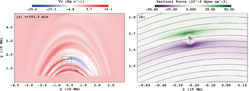
Figure 1: At $t\approx 100$ minutes, we show the $x$-velocity component at left. Right panel: zoomed view on the local signed vertical total force.

Because the heating formula for $H_{1}$ affects only a selection of loops fully contained interior to our simulation domain, this part of the arcade witnesses increased densities and temperatures, with maximum values of 2.1 MK after 9 minutes of added heating. Despite loop-aligned thermal conduction transporting energy to the dense coronal plasma around the apexes, temperatures then start to reduce slowly, while the densities still keep increasing. The locally heated arcade system continues to evolve, and only after about 100 minutes of sustained heating, the temperature at a height of 16.5 Mm suddenly declines drastically to 0.04 MK, slightly off-center. A small condensation segment with a density $5.6\times 10^{10}$ cm^-3 suddenly comes forth around the apexes of a strand of magnetic loops. Figure 1 shows the velocity field, and the (signed) vertical total force with gravity, Lorentz force and pressure gradient in a zoomed view on the blob forming. The overall perturbed force field extends over 1 Mm in width, and has dominant about equal and in-phase pressure and Lorentz force contributions and induces field variations on neighboring fieldlines, which aid in triggering sympathetic condensations. Indeed, after this first localized condensation event, similar condensation processes continuously arise on both ends of the first condensation. Due to the broken symmetry, we observe this to extend into coronal loops on either side of the first affected loop strand, and this results into the larger scale condensation to look like a zigzag rope (like in panel (c) of Fig. 2). What happens next is a spectacular display of fragmenting, forming, relocating plasma blobs, since the cool plasma condensations spontaneously loose their balance between existing forces (gravity, magnetic, and gas pressure gradients), and start to slide down slowly along magnetic field lines. In the online movies, one can see how at about 118 minutes, the big zigzag condensation begins to split into several smaller blobs, descending along both rims of the magnetic field. After about 160 minutes, also due to the depletion of plasma in these loops, the subsequent phase seems less vigorous. Similar phases can be found in observations (Antolin et al., 2010; Antolin & Rouppe van der Voort, 2012), and are interpreted as ‘limit cycles of loop evolution’ by Müller et al. (2003).

Our simulation shows new features related to blob destruction. In particular, at 167 minutes, at a height of 10 Mm and horizontal position of $x=-21$ Mm, a small baby blob with a number density of $9.0\times 10^{9}$ cm^-3 and temperature 0.55 MK, forms in a first slowly upflowing part of a strand of loops, where another bigger blob has just descended. This blob has an upward velocity of 10 km s^-1, but then gets destroyed by a hot inflow from the other side due to the heating-induced evaporation at the other loop footpoint. This is supported by an online movie.

At the overall effective resolution, any individual grid cell where the number density exceeds $7.0\times 10^{9}{\mathrm{cm}}^{-3}$, the temperature drops below 0.1 MK in the corona is labeled as in a coronal rain blob. These threshold values are suggested by observational findings (Hirayama, 1985) and other numerical simulations (Müller et al., 2005; Antolin et al., 2010). To count the instantaneous amount of blobs present at one time, we then identify the total number of blobs by assuming that all connected labeled pixels actually compose a single blob. In that way, we can report on the instantaneous amount of coronal rain blobs and the centroid $(x_{c},y_{c})$ coordinates of each blob. The local magnetic field vector defines directions along and perpendicular to the field line. Along these directions, the length and width of the blob are quantified. However, since the resolution of our numerical simulation (78 km) is much higher than current observational resolutions, e.g., 150 km of CRISP (Antolin & Rouppe van der Voort, 2012), the number of identified blobs in the simulation is larger than that found in comparable observations. For the sake of direct comparison with the observations, we also do this at a resolution of 200 km. This operation combines neighboring blobs and occasionally overlooks blobs with sizes below this resolution.

Fig. 3(a) shows that the total mass of all blobs as function of time is nearly identical between the numerical resolution (dashed curve) and the observational resolution (solid curve), while the former slightly exceeds the latter. The difference between observations versus simulations is more pronounced in Fig. 3(b) showing the actual numbers of blobs. While actual blob numbers can go over 100 at certain times, still when viewing them with observational resolution as fewer (less than 20) blobs, the total mass basically remains the same between different resolutions. This means that while current coronal rain related mass estimates from observations are likely to be correct, there are still a great quantity of small unresolved blobs in present-day observations. After the first condensation seen at $t\approx 100$ minutes, Fig. 3(a) shows that in the next 29 minutes, still before the first descending blob crashes into the transition region, the mass accumulation of the blobs scales at a rapid rate of 6.7 g cm^-1 s^-1. To quantify a true mass drain rate, we could adopt an average size in $z$ of 400 km as the average width, making the mass drain rate about $3\times 10^{9}$ g s^-1, very similar to observational results (Antolin & Rouppe van der Voort, 2012). Snapshots of density and temperature at times $t\approx 136$ and $t\approx 152$ minutes are shown in Fig. 2, where selected blobs are labeled by numbers, used in the further discussion.

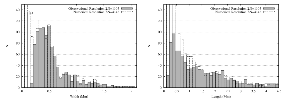
Figure 4: (a) and (b) show the distribution function of width and length, respectively, at numerical and observational resolution.

A large variety of blob appearances are found during the whole coronal rain process. By treating every snapshot between $t\approx 100$ and $t\approx 200$ at a time interval of 43 seconds as an individual observation, we can easily obtain statistically meaningful distribution functions of blob width and length. This is quantified in Fig. 4 where we again contrast findings based on the numerical resolution with the observational resolution. The width of the blobs reveal the intrinsic cross section of a strand of loops with nearly synchronous evolution. Recent results from triple-filter analysis of the finest coronal loops analyzed in TRACE images found elementary loop strands with isothermal cross sections of $\approx 1000-2000$ km (Aschwanden & Nightingale, 2005). Similar values of sympathetic loop strand widths can be seen in the horizontal velocity map in Fig. 1, are also seen in the perturbed force view and return in the distribution function of the obtained blob widths in panel (a) of Fig. 4. Although the width of such strands and blobs can reach the maximum value of 2000 km, these huge blobs will be separated during the propagation process into small fragments. This is again resulting from significant differences in the diverse forces acting along their body. The width histogram in Fig. 4(a) also shows that the vast majority of blobs possess widths like $\approx 200-1000$ km with an average 400 km, in direct correspondence with recent observational results from Antolin & Rouppe van der Voort (2012).

4 DYNAMICS OF BLOBS

The velocity structure at $t\approx 100$ minutes is shown in Fig. 1, at the same time as the density and temperature panels (a) and (b) of Fig. 2. In the velocity plot, one identifies the condensation where two strong opposite inflows with a maximum relative velocity of 68.7 km s^-1 are siphoned towards the condensation site from both sides. This coincides with a dramatic evacuation of a loop strand caused by the catastrophic cooling. The thermodynamic evolution rapidly refills the local empty loops with hot and rarefied plasma. These fast inflows and the density variation they create, first realize a pressure difference across the two sides of the off-center blob, which levitates the newborn blob against gravity. This first phase impedes the descending process of newborn blobs. However, after a short time the inflows become slower, and while the blob density increases, this previous pressure difference gradually fades away. Therefore, they ultimately start to accelerate quickly downwards.

To explain how a full loop strand ultimately shows blobs that appear like comet-shaped or $V$-like features during propagation (Antolin et al., 2010; Antolin & Verwichte, 2011), we note that within a loop strand of finite extent (say few hundred km in width), a first small condensation functions like the seed for a larger blob. In this growth, the condensation process appears to extend from the first blob onwards due to the synchronous temperature evolution in a wider loop strand (Klimchuk et al., 2010). This means that while the firstly formed condensation may already have evolved beyond the phase where it experiences levitating pressure support, the condensation segments formed later at the edge of the blob are still locally supported against gravity by the pressure difference due to the fast siphon inflows. As a result, the large, growing blob gets deformed as a whole into a comet-shaped pattern, like the blobs labeled with numbers 3-7 of Fig. 2. During their propagation towards the arcade footpoints, catastrophic cooling further sets in in the tail of these blobs, and blobs will be elongated by continuously forming condensations on the way down. Furthermore, as the gravitational acceleration varies with height, an effect accounted for in our external $y$-stratified gravitational field, the blob will also become elongated due to being stretched by the differential component of gravity along the curved magnetic field. Therefore, the length histogram in panel (b) of Fig. 4 presents an average of 850 km for coronal rain blobs, but shows a wide range of lengths going from 200 km to exceeding 4500 km, a fact confirmed by observations (Schrijver, 2001; Antolin & Rouppe van der Voort, 2012). Zoomed views on selected blobs in Fig. 2 show the local temperature structure, with conduction-dominated regions around the blobs. The temperatures of these local transition regions are around 0.6 MK.

We obtain a broad distribution of projected velocities, ranging from few km s^-1 to the high velocity of descending blobs going up to more than 60 km s^-1. Panel (c) of Fig. 3 shows a scatter plot of the horizontal centroid $x_{c}$-position of the blobs versus their in-plane projected velocity, signed by vertical velocity. This is done at the observational resolution, and in this view one can trace individual blobs appearing in multiple snapshots. Panel (d) of Fig. 3 shows a scatter plot of height $y_{c}$ of the blobs versus their projected velocity, now signed with $v_{x}$. Since the velocities are generally height dependent, the dashed curve in panel (d) of Fig. 3 denotes the path that a blob would follow if it were falling from a height of 30 Mm, subject to an acceleration of 0.18 km s^-2, the average effective gravity for a loop whose height to half baseline ratio is 30 (Mm)/26 (Mm). We note that most of the measurements are located below the dashed curve, like those for blob 6 and 7. This scenario suggests a role for other forces than gravity, like gas pressure as suggested by previous 1D numerical simulations (Müller et al., 2003, 2004, 2005).

Close to the lower parts above the transition region of the arcade, strong deceleration of individual blobs are sometimes observed (Antolin & Rouppe van der Voort, 2012), which is explained by the increase of gas pressure there from the higher local densities. The solid lines connecting the points of individual blobs 3 and 4 in panels (c) and (d) of Fig. 3 show these strong decelerations happening right above the transition region. Decelerated by this pressure gradient, the leading descending blob part could be caught up by a later faster descending blob part (as in 1D studies from (Müller et al., 2005)) and merge to one heavier blob. At about 152 minutes, in panel (e) of Fig. 2, at a height of 7.1 Mm and horizontal position of $x=22.5$ Mm, we find that in the trail of a formerly descending blob, a small blob (number 8) appears and stays there supported by the large pressure gradient. Meanwhile, in the same strand, another blob (number 9) forms above the number 8 and moves towards it with velocity of 26 km s^-1. They collide, merge and produce a heavier blob, which finally falls down to the transition region 4 minutes later. A movie with a zoomed view on this process is available online.

In panel (e) of Fig. 2, two blobs in the same flux loop strand, numbered 10 and 11, approach each other because of the significant pressure difference across them, as extremely low gas pressure is induced by catastrophic cooling in between them, and the gas pressure outside enforces their mutual approach. This kind of situation can even suck a blob upwards, ascending and crossing the apexes of loops, e.g. this is what happens to the blob number 1(2) in panel (e) of Fig. 2, which shares the same strand with blob number 5. In panels (c) and (d) of Fig. 3, the scatter velocity plots versus height and $x$-position show us this clearly when inspecting the traces of blob 1(2) and blob 5. When blob 5 descends to the footpoint, blob 1(2) is siphoned to ascend from the right rim and over to the left rim along the magnetic field lines.

5 Conclusions

We simulate the initial formation and the long-term sustainment of the enigmatic coronal rain phenomenon for the first time in a realistic multi-dimensional magnetic configuration. In the over 80 minutes physical time, we collect enough statistics to quantify blob widths, lengths which average 400 km, 800 km, and the velocity distribution from small values to 65 km s^-1. Our virtual coronal rain display features the deformation of blobs into $V$-shapes, interactions of blobs due to mostly pressure-mediated levitations, and gives the first views on blobs which evaporate in situ, or get siphoned over the apex of the background arcade. We will perform parameter studies for similar arcade configurations, varying field strength, overall topology and the role of magnetic shear.

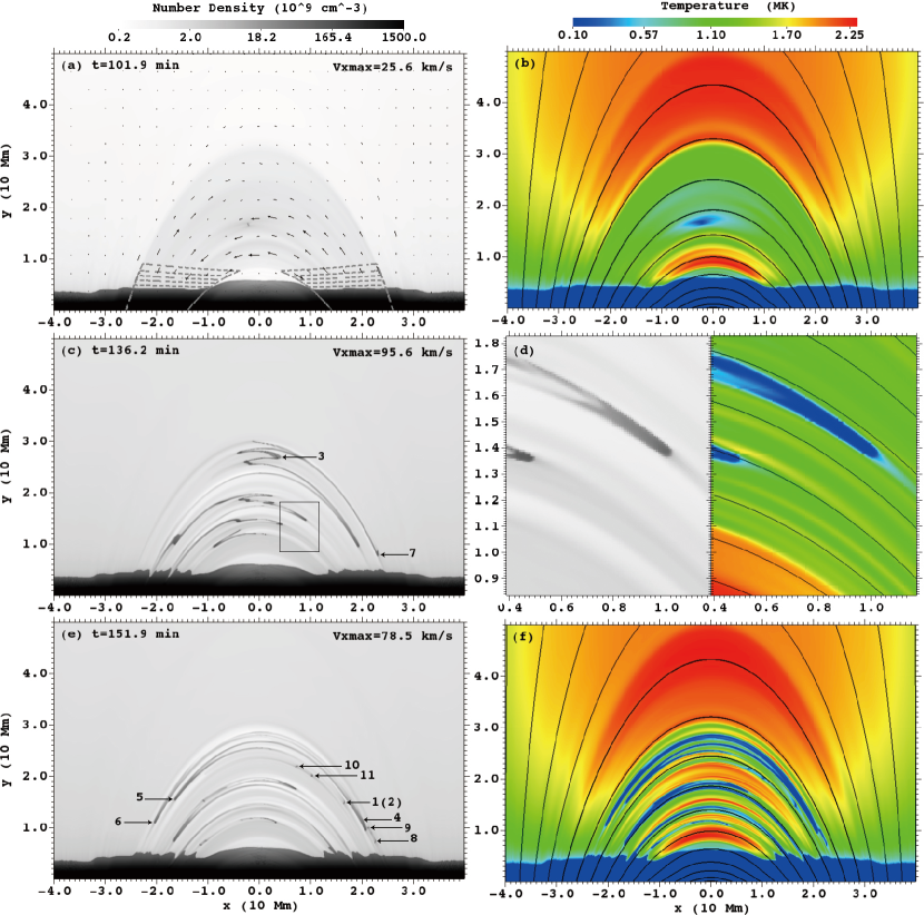
Figure 2: Snapshots at t=100 (first row), 136 (second row) and 152 minutes (third row). At left: density. At right: temperature and magnetic field lines. Localized heating is shown as contours in panel (a) and velocity arrows. Panel (d) shows the thermal stucture, zooming into blobs in panel (c).

Figure 3: (a)Total mass versus time with numerical resolution (dashed curve) and observational resolution (solid curve); (b) number of blobs; (c) scatter plot of projected velocity with sign of $v_{y}$ versus $x$-axis value; (d) scatter plot of projected velocity with sign of $v_{x}$ versus height of blobs. The dashed curve denotes the path that a blob would follow if falling from a height of 30 Mm and subject to an acceleration of 0.18 km s^-2. All solid curves connecting points in (c) and (d) show the trace of several blobs, numbered from 1(2) to 7.

References

- Antiochos & Klimchuk (1991) Antiochos, S. K., & Klimchuk, J. A. 1991, ApJ, 378, 372
- Antiochos et al. (1999) Antiochos, S. K., MacNeice, P. J., Spicer, D. S., & Klimchuk, J. A. 1999, ApJ, 512, 985
- Antolin & Rouppe van der Voort (2012) Antolin, P., & Rouppe van der Voort, L. 2012, ApJ, 745, 152
- Antolin et al. (2010) Antolin, P., Shibata, K., & Vissers, G. 2010, ApJ, 716, 154
- Antolin & Verwichte (2011) Antolin, P., & Verwichte, E. 2011, ApJ, 736, 121
- Aschwanden & Nightingale (2005) Aschwanden, M. J., & Nightingale, R. W. 2005, ApJ, 633, 499
- De Groof et al. (2005) De Groof, A., Bastiaensen, C., Müller, D. A. N., Berghmans, D., & Poedts, S. 2005, A&A, 443, 319
- De Groof et al. (2004) De Groof, A., Berghmans, D., van Driel-Gesztelyi, L., & Poedts, S. 2004, A&A, 415, 1141
- Field (1965) Field, G. B. 1965, ApJ, 142, 531
- Goldsmith (1971) Goldsmith, D. W. 1971, Sol. Phys., 19, 86
- Hirayama (1985) Hirayama, T. 1985, Sol. Phys., 100, 415
- Kamio et al. (2011) Kamio, S., Peter, H., Curdt, W., & Solanki, S. K. 2011, A&A, 532, A96
- Keppens et al. (2012) Keppens, R., Meliani, Z., van Marle, A. J., Delmont, P., Vlasis, A., & van der Holst, B. 2012, JCP, 231, 718
- Karpen et al. (2001) Karpen, J. T., Antiochos, S. K., Hohensee, M., Klimchuk, J. A., & MacNeice, P. J. 2001, ApJ, 553, L85
- Kawaguchi (1970) Kawaguchi, I. 1970, PASJ, 22, 405
- Klimchuk et al. (2010) Klimchuk, J. A., Karpen, J. T., & Antiochos, S. K. 2010, ApJ, 714, 1239
- Leroy (1972) Leroy, J.-L. 1972, Sol. Phys., 25, 413
- Müller et al. (2005) Müller, D. A. N., De Groof, A., Hansteen, V. H., & Peter, H. 2005, A&A, 436, 1067
- Müller et al. (2003) Müller, D. A. N., Hansteen, V. H., & Peter, H. 2003, A&A, 411, 605
- Müller et al. (2004) Müller, D. A. N., Peter, H., & Hansteen, V. H. 2004, A&A, 424, 289
- Mok et al. (1990) Mok, Y., Drake, J. F., Schnack, D. D., & van Hoven, G. 1990, ApJ, 359, 228
- Mok et al. (2005) Mok, Y., Mikić, Z., Lionello, R., & Linker, J. A. 2005, ApJ, 621, 1098
- O’Shea et al. (2007) O’Shea, E., Banerjee, D., & Doyle, J. G. 2007, A&A, 475, L25
- Parker (1953) Parker, E. N. 1953, ApJ, 117, 431
- Schrijver (2001) Schrijver, C. J. 2001, Sol. Phys., 198, 325
- Xia et al. (2011) Xia, C., Chen, P. F., Keppens, R., & van Marle, A. J. 2011, ApJ, 737, 27
- Xia et al. (2012) Xia, C., Chen, P. F., & Keppens, R. 2012, ApJ, 748, L26