On Finite Block-Length Quantization Distortion

Abstract

We investigate the upper and lower bounds on the quantization distortions for independent and identically distributed sources in the finite block-length regime. Based on the convex optimization framework of the rate-distortion theory, we derive a lower bound on the quantization distortion under finite block-length, which is shown to be greater than the asymptotic distortion given by the rate-distortion theory. We also derive two upper bounds on the quantization distortion based on random quantization codebooks, which can achieve any distortion above the asymptotic one. Moreover, we apply the new upper and lower bounds to two types of sources, the discrete binary symmetric source and the continuous Gaussian source. For the binary symmetric source, we obtain the closed-form expressions of the upper and lower bounds. For the Gaussian source, we propose a computational tractable method to numerically compute the upper and lower bounds, for both bounded and unbounded quantization codebooks. Numerical results show that the gap between the upper and lower bounds is small for reasonable block length and hence the bounds are tight.

Key Words: Rate-distortion, finite block-length, quantization, binary symmetric source, Gaussian source.

I Introduction

The rate distortion theory provides an achievable asymptotic lower bound on the distortion of the lossy quantization, as the block length of the source sequence approaches infinity. This bound is described by a single-symbol probability transition function between the original alphabet and the reconstruction alphabet, which produces the minimum asymptotic distortion provided that the mutual information is below the quantization rate. For sufficiently large block length, any distortion above the asymptotic bound can be achieved; and any distortion below the asymptotic bound cannot be achieved for any block length [1]. Existing works on the rate distortion focuses on either the rate-distortion functions of various types of sources [2, 3, 4, 5, 6, 7], or the analysis of various exponents as the quantization block length approaches infinity [8, 9, 10, 11, 12].

On the other hand, in the non-asymptotic regime, up till now there has been no analysis on the lower bounds for the vector quantization in the finite block-length regime, even for i.i.d. sources. Note that, since the rate-distortion theory provides an asymptotic achievable lower bound, any meaningful lower bound in the finite block-length regime should be larger than this asymptotic lower bound. Also, to the best of our knowledge, the only upper bound for random quantization codebook is provided in [9]. This upper bound can be improved.

In this paper, we derive new upper and lower bounds on the optimal quantization error in the finite block length regime. More specifically, based on the convex optimization formulation of the rate-distortion problem, we derive a lower bound for the quantization distortion, which is shown to be larger than the asymptotic distortion and thus is non-trivial. Using this lower bound, we analyze the duality between the quantization distortion and the error probability of the equivalent channel characterized by the optimal probability transition function. We further specialize the lower bounds to cases where the codewords are bounded and where the source is symmetric, respectively. We then provide two improved upper bounds on the vector quantization distortion assuming random quantization codebooks. It is shown that any quantization distortion above the asymptotic lower bound can be achieved by the proposed upper bounds.

Furthermore, we apply new upper and lower bounds to two types of sources, the discrete binary symmetric source and the continuous Gaussian source. For the binary symmetric source, we provide closed-form expressions for the upper and lower bounds. For the Gaussian source, we further analyze the upper and lower bounds for codebooks with bounded and unbounded codewords, respectively, and provide an efficient method to compute these bounds.

The remainder of this paper is organized as follows. In Section II, we introduce the problem formulation. In Sections III and IV, we derive lower and upper bounds for the optimal quantization distortion, respectively. In Sections V and VII, we specialize the new bounds to the binary symmetric source and identically and the Gaussian source, respectively. Finally, Section VIII contains the concluding remarks. All proofs are relegated to the Appendix.

II Background and Problem Statement

Consider a memoryless source with an original symbol alphabet ${\cal X}$, which is to be reconstructed using a reconstruction symbol alphabet ${\cal Y}$. For each pair $(x,y)\in{\cal X}\times{\cal Y}$, let $d(x,y)$ denote the distortion of representing symbol $x$ using symbol $y$. Note that $d(x,y)\geq 0$ for all $(x,y)\in{\cal X}\times{\cal Y}$. Assume that the original symbol $x\in{\cal X}$ has a probability density function (pdf) $p(x)$. Let $q(y|x)$ denote the conditional pdf of the reconstruction symbol $y\in{\cal Y}$ given the original symbol $x\in{\cal X}$. Define $D(q)$ as the expected distortion of the conditional pdf $q(y|x)$, given by

$$D(q)\stackrel{{\scriptstyle\triangle}}{{=}}\mathbb{E}_{(x,y)\sim p(x)q(y|x)}\Big{(}d(x,y)\Big{)}=\int\int p(x)q(y|x)d(x,y)dxdy.$$ (1)

We adopt conventional notations $H(\cdot)$, $H(\cdot|\cdot)$, and $I(\cdot;\cdot)$ to denote the entropy, conditional entropy, and mutual information, respectively. We define $I(q)\stackrel{{\scriptstyle\triangle}}{{=}}I(X;Y)$ as the mutual information between $X$ and $Y$ under the conditional pdf $q(y|x)$.

Consider a length-$n$ source symbol block ${\mbox{\boldmath$x$}}\stackrel{{\scriptstyle\triangle}}{{=}}(x_{1},x_{2},...,x_{n})\in{\cal X}^{n}$ that is to be reconstructed using a length-$n$ reconstruction symbol block ${\mbox{\boldmath$y$}}\stackrel{{\scriptstyle\triangle}}{{=}}(y_{1},y_{2},...,y_{n})\in{\cal Y}^{n}$. Define the following distortion metric between $x$ and $y$,

$$d({\mbox{\boldmath$x$}},{\mbox{\boldmath$y$}})\stackrel{{\scriptstyle\triangle}}{{=}}\frac{\sum^{n}_{i=1}d(x_{i},y_{i})}{n}.$$ (2)

Then the expected distortion with respect to the reconstructing pdf $q({\mbox{\boldmath$y$}}|{\mbox{\boldmath$x$}})$ is

$$D(q)\stackrel{{\scriptstyle\triangle}}{{=}}\mathbb{E}_{({\mbox{\boldmath$x$}},{\mbox{\boldmath$y$}})\sim p({\mbox{\boldmath$x$}})q({\mbox{\boldmath$y$}}|{\mbox{\boldmath$x$}})}\Big{(}d({\mbox{\boldmath$x$}},{\mbox{\boldmath$y$}})\Big{)}=\int\int p({\mbox{\boldmath$x$}})q({\mbox{\boldmath$y$}}|{\mbox{\boldmath$x$}})d({\mbox{\boldmath$x$}},{\mbox{\boldmath$y$}})d{\mbox{\boldmath$y$}}d{\mbox{\boldmath$x$}}.$$ (3)

We consider reconstructing ${\mbox{\boldmath$x$}}\in{\cal X}^{n}$ using a size-$Q$ quantization codebook ${\cal Y}_{Q}\stackrel{{\scriptstyle\triangle}}{{=}}\{{\mbox{\boldmath$y$}}_{1},{\mbox{\boldmath$y$}}_{2},...,{\mbox{\boldmath$y$}}_{Q}\}\subseteq{\cal Y}^{n}$. Let $q_{Q}({\mbox{\boldmath$y$}}_{j}|{\mbox{\boldmath$x$}})$ be the probability of quantizing $x$ to ${\mbox{\boldmath$y$}}_{j}$. Define the distortion with respect to the quantization function $q_{Q}({\mbox{\boldmath$y$}}_{j}|{\mbox{\boldmath$x$}})$ as

$$D^{n}(q_{Q})=\int p({\mbox{\boldmath$x$}})\sum^{Q}_{j=1}q_{Q}({\mbox{\boldmath$y$}}_{j}|{\mbox{\boldmath$x$}})d({\mbox{\boldmath$x$}},{\mbox{\boldmath$y$}}_{j})d{\mbox{\boldmath$x$}}.$$ (4)

It is easily seen that the distortion $D^{n}(q_{Q})$ is minimized when $q_{Q}({\mbox{\boldmath$y$}}_{j^{*}}|{\mbox{\boldmath$x$}})=1$, where

$$j^{*}=\arg\min_{1\leq k\leq Q}d({\mbox{\boldmath$x$}},{\mbox{\boldmath$y$}}_{k}),$$ (5)

and $q_{Q}({\mbox{\boldmath$y$}}_{j}|{\mbox{\boldmath$x$}})=0$ for $j\neq j^{*}$. If there are multiple codewords satisfying (5), then $j^{*}$ is the smallest index $j$ among such codewords. Define ${\cal R}_{j}$ as the quantization region of ${\mbox{\boldmath$y$}}_{j}$, given by

$${\cal R}_{j}\stackrel{{\scriptstyle\triangle}}{{=}}\{{\mbox{\boldmath$x$}}:q_{Q}({\mbox{\boldmath$y$}}_{j}|{\mbox{\boldmath$x$}})=1\},\ \mbox{or}\ \ q_{Q}({\mbox{\boldmath$y$}}_{j}|{\mbox{\boldmath$x$}})=\mathbf{1}_{\{{\mbox{\boldmath$x$}}\in{\cal R}_{j}\}}.$$ (6)

Note that the subsets ${\cal R}_{j}$, $1\leq j\leq Q$, are non-overlapping and $\cup^{Q}_{j=1}{\cal R}_{j}={\cal X}^{n}$.

We denote $D^{n}({\cal Y}_{Q})\stackrel{{\scriptstyle\triangle}}{{=}}D^{n}(q_{Q})$ as the quantization distortion of the codebook ${\cal Y}_{Q}$, and summarize the above arguments as follows.

Theorem 1

Consider the non-overlapping subsets ${\cal R}_{j}$, $1\leq j\leq Q$, of ${\cal X}^{n}$ given by (6). Then, for any quantization probability function $\tilde{q}_{Q}$,

$$D^{n}(\tilde{q}_{Q})\geq D^{n}({\cal Y}_{Q})=\sum^{Q}_{j=1}\int_{{\cal R}_{j}}p({\mbox{\boldmath$x$}})d({\mbox{\boldmath$x$}},{\mbox{\boldmath$y$}}_{j})d{\mbox{\boldmath$x$}}.$$ (7)

$\hfill\Box$

The rate-distortion theory provides an asymptotic lower bound to the quantization distortion $D^{n}(q_{Q})$ in (4) as the block length $n$ approaches infinity. Let the size of the quantization codebook ${\cal Y}_{Q}$ be $Q=2^{nR}$. According to the rate-distortion theory, any distortion $D$ can be achieved if $D>D(R)$, where

$$D(R)\stackrel{{\scriptstyle\triangle}}{{=}}\min_{q(y|x),I(q)\leq R}D(q),$$ (8)

for sufficiently large block length $n$; and any distortion $D<D(R)$ is not achievable for any block length $n$. Note that in (8), $q(y|x)$ is the single-alphabet conditional pdf.

The rate distortion theory provides a lower bound to the quantization error as the block length $n$ approaches infinity. Such an asymptotic bound typically cannot accurately approximate the distortion for finite block length. In this work, we aim to obtain upper and lower bounds for the quantization distortion $D^{n}(q_{Q})$ in (4) for finite $n$.

In the remainder of this paper, let $\hat{q}(y|x)$ be the optimal solution to $q(y|x)$ which minimizes the distortion $D(q)$ for infinite quantization block length, i.e., the optimal solution to the rate-distortion problem (8). We denote $D^{*}\stackrel{{\scriptstyle\triangle}}{{=}}D(\hat{q})$ as the resulting minimum distortion from the rate-distortion theory. For length-$n$ symbol blocks ${\mbox{\boldmath$x$}}=(x_{1},x_{2},...,x_{n})$ and ${\mbox{\boldmath$y$}}=(y_{1},y_{2},...,y_{n})$, we define the following product pdf of the optimal quantization function $\hat{q}(y|x)$,

$$\hat{q}({\mbox{\boldmath$y$}}|{\mbox{\boldmath$x$}})\stackrel{{\scriptstyle\triangle}}{{=}}\prod^{n}_{i=1}\hat{q}(y_{i}|x_{i}).$$ (9)

III A Lower Bound on Quantization Distortion

In this section, we derive a lower bound on the quantization distortion $D^{n}(q_{Q})$ in (4). We start from the convex optimization formulation of the rate distortion problem in (8).

III-A Convex Optimization Formulation of the Rate Distortion Problem

The rate-distortion problem in (8) can be expressed as

$$\min_{q(y|x)}\int\int p(x)q(y|x)d(x,y)dxdy,$$

s.t. $$I(X;Y)=\int\int p(x)q(y|x)\log\frac{q(y|x)}{\int_{{\cal X}}p(x^{\prime})q(y|x^{\prime})dx^{\prime}}dxdy\leq R,$$ (10)

$$\int q(y|x)dy=1,\ x\in{\cal X}.$$

Note that the mutual information $I(X;Y)$ is a convex function in terms of $q(y|x)$ for a fixed $p(x)$ [1]. Hence the above is a convex optimization problem. The Lagrangian form of (III-A) can be written as

$$J(q,\lambda,v) = \int\int p(x)q(y|x)d(x,y)dxdy+\int v(x)\Big{(}\int q(y|x)dy-1\Big{)}dx$$ (11)

$$\ \ +\lambda\Big{(}\int\int p(x)q(y|x)\log\frac{q(y|x)}{\int p(x^{\prime})q(y|x^{\prime})dx^{\prime}}dxdy-R\Big{)}.$$

We then have

$$\frac{\partial J}{\partial q(y|x)}=p(x)d(x,y)+\lambda p(x)\log\frac{q(y|x)}{q(y)}+v(x),$$ (12)

where $q(y)=\int_{{\cal X}}p(x)q(y|x)dx$. Let $\hat{q}(y)=\int_{{\cal X}}p(x)\hat{q}(y|x)dx$, where $\hat{q}(y|x)$ is an optimal solution to (8). Then, by the KKT condition, we have

$$\frac{\partial J}{\partial q(y|x)}\Big{|}_{q(y|x)=\hat{q}(y|x)}=0\ \mbox{for}\ \hat{q}(y|x)>0,\ \mbox{and}\ \frac{\partial J}{\partial q(y|x)}\Big{|}_{q(y|x)=\hat{q}(y|x)}\geq 0\ \mbox{for}\ \hat{q}(y|x)=0,$$ (13)

which can be compactly written as

$$\hat{q}(y|x)\frac{\partial J}{\partial q(y|x)}\Big{|}_{q(y|x)=\hat{q}(y|x)}=0.$$ (14)

The Slater condition [13] for the convex optimization problem says that the dual gap is zero if there is a feasible conditional pdf $q(y|x)$ such that $I(q)<R$. This can be easily verified since we can set $q(y|x)=1$ for $y=y_{0}$ and $q(y|x)=0$ otherwise for all $x$, for some fixed $y_{0}$, such that $I(q)=I(X;Y)=0$. Therefore, for the optimal solution to (III-A) the duality gap is zero. Thus, we have the following result.

Theorem 2

Let $\hat{q}(y|x)$ be an optimal conditional pdf, $\hat{q}(y)$ be the corresponding marginal pdf of $y$, and $\hat{\lambda}$ and $\hat{v}(x)$ be the optimal dual variables. Let $\hat{q}(x|y)=\frac{p(x)\hat{q}(y|x)}{\int_{x}p(x)q(y|x)dx}$. Then, we have the following conditions to characterize the optimal solution to (III-A):

$$p(x)d(x,y)+\hat{\lambda}p(x)\log\frac{\hat{q}(y|x)}{\hat{q}(y)}+\hat{v}(x) = 0,\ \mbox{for}\ \hat{q}(y|x)>0;$$ (15)

$$p(x)d(x,y)+\hat{\lambda}p(x)\log\frac{\hat{q}(y|x)}{\hat{q}(y)}+\hat{v}(x) \geq 0,\ \mbox{for}\ \hat{q}(y|x)=0;$$ (16)

$$p(x)\hat{q}(y|x)d(x,y)+\hat{\lambda}p(x)\hat{q}(y|x)\log\frac{\hat{q}(y|x)}{\hat{q}(y)}+\hat{q}(y|x)\hat{v}(x) = 0,\ x\in{\cal X},y\in{\cal Y};$$ (17)

$$\hat{\lambda}\Big{(}\int\int p(x)\hat{q}(y|x)\log\frac{\hat{q}(y|x)}{\hat{q}(y)}dxdy-R\Big{)} = 0;$$ (18)

$$\hat{v}(x)\Big{(}\int\hat{q}(y|x)dy-1\Big{)} = 0,\ x\in{\cal X}.$$ (19)

$\hfill\Box$

III-B A Lower Bound on Distortion

The following result gives a lower bound on the distortion $D^{n}(q)$ for block size $n$ and a given reconstruction conditional pdf $q({\mbox{\boldmath$y$}}|{\mbox{\boldmath$x$}})$.

Theorem 3

Let $\hat{q}(y|x)$ be an optimal conditional pdf, and $\hat{q}(y)$ be the corresponding marginal pdf of $y$, and $\hat{\lambda}$ and $\hat{v}(x)$ be the optimal dual variables for the rate-distortion problem (III-A). Then, for any reconstruction conditional pdf $q({\mbox{\boldmath$y$}}|{\mbox{\boldmath$x$}})$, we have

$$D^{n}(q)-D^{*}\geq\frac{\hat{\lambda}}{n}\Big{(}nI(\hat{q})-\int\int p({\mbox{\boldmath$x$}})q({\mbox{\boldmath$y$}}|{\mbox{\boldmath$x$}})\log\frac{\hat{q}({\mbox{\boldmath$x$}}|{\mbox{\boldmath$y$}})}{p({\mbox{\boldmath$x$}})}d{\mbox{\boldmath$y$}}d{\mbox{\boldmath$x$}}\Big{)};$$ (20)

and the equality holds if $\hat{q}(y|x)>0$ for all $x\in{\cal X}$ and $y\in{\cal Y}$.

Proof:

Since the source is memoryless, we have that $p({\mbox{\boldmath$x$}})=\prod^{n}_{i=1}p(x_{i})$, and thus

$$p({\mbox{\boldmath$x$}})d({\mbox{\boldmath$x$}},{\mbox{\boldmath$y$}})=\prod^{n}_{j=1}p(x_{j})\frac{\sum^{n}_{i=1}d(x_{i},y_{i})}{n}=\frac{1}{n}\sum^{n}_{i=1}\prod_{j\neq i}p(x_{j})p(x_{i})d(x_{i},y_{i}).$$ (21)

From Theorem 2, it follows that

$$p(x_{i})d(x_{i},y_{i})\geq-\hat{\lambda}p(x_{i})\log\frac{\hat{q}(y_{i}|x_{i})}{\hat{q}(y_{i})}-\hat{v}(x_{i}).$$ (22)

Substituting (22) into (21), we have

$$p({\mbox{\boldmath$x$}})d({\mbox{\boldmath$x$}},{\mbox{\boldmath$y$}}) \geq -\frac{1}{n}\sum^{n}_{i=1}\prod_{j\neq i}p(x_{j})\hat{\lambda}p(x_{i})\log\frac{\hat{q}(y_{i}|x_{i})}{\hat{q}(y_{i})}-\frac{1}{n}\sum^{n}_{i=1}\prod_{j\neq i}p(x_{j})\hat{v}(x_{i})$$ (23)

$$= -\frac{\hat{\lambda}}{n}p({\mbox{\boldmath$x$}})\log\frac{\hat{q}({\mbox{\boldmath$y$}}|{\mbox{\boldmath$x$}})}{\hat{q}({\mbox{\boldmath$y$}})}-\frac{1}{n}\sum^{n}_{i=1}\prod_{j\neq i}p(x_{j})\hat{v}(x_{i}).$$

Therefore, we have,

$$D^{n}(q) = \int\int p({\mbox{\boldmath$x$}})q({\mbox{\boldmath$y$}}|{\mbox{\boldmath$x$}})d({\mbox{\boldmath$x$}},{\mbox{\boldmath$y$}})d{\mbox{\boldmath$x$}}d{\mbox{\boldmath$y$}}$$ (24)

$$\geq -\frac{\hat{\lambda}}{n}\int\int p({\mbox{\boldmath$x$}})q({\mbox{\boldmath$y$}}|{\mbox{\boldmath$x$}})\log\frac{\hat{q}({\mbox{\boldmath$y$}}|{\mbox{\boldmath$x$}})}{\hat{q}({\mbox{\boldmath$y$}})}d{\mbox{\boldmath$x$}}d{\mbox{\boldmath$y$}}-\frac{1}{n}\int\int q({\mbox{\boldmath$y$}}|{\mbox{\boldmath$x$}})\sum^{n}_{i=1}\prod_{j\neq i}p(x_{j})\hat{v}(x_{i})d{\mbox{\boldmath$x$}}d{\mbox{\boldmath$y$}}$$

$$= -\frac{\hat{\lambda}}{n}\int\int p({\mbox{\boldmath$x$}})q({\mbox{\boldmath$y$}}|{\mbox{\boldmath$x$}})\log\frac{\hat{q}({\mbox{\boldmath$x$}}|{\mbox{\boldmath$y$}})}{p({\mbox{\boldmath$x$}})}d{\mbox{\boldmath$x$}}d{\mbox{\boldmath$y$}}-\frac{1}{n}\int\sum^{n}_{i=1}\prod_{j\neq i}p(x_{j})\hat{v}(x_{i})d{\mbox{\boldmath$x$}}.$$

On the other hand, using a similar argument as above and noting that (14) holds for the optimal solution $\hat{q}(y|x)$, we have that

$$D^{n}(\hat{q}) = -\frac{\hat{\lambda}}{n}\int\int p({\mbox{\boldmath$x$}})\hat{q}({\mbox{\boldmath$y$}}|{\mbox{\boldmath$x$}})\log\frac{\hat{q}({\mbox{\boldmath$y$}}|{\mbox{\boldmath$x$}})}{\hat{q}({\mbox{\boldmath$y$}})}d{\mbox{\boldmath$x$}}d{\mbox{\boldmath$y$}}-\frac{1}{n}\int\sum^{n}_{i=1}\prod_{j\neq i}p(x_{j})\hat{v}(x_{i})d{\mbox{\boldmath$x$}}$$ (25)

$$= -\hat{\lambda}I(\hat{q})-\frac{1}{n}\int\sum^{n}_{i=1}\prod_{j\neq i}p(x_{j})\hat{v}(x_{i})d{\mbox{\boldmath$x$}}.$$

Recall that $D^{*}=D^{n}(\hat{q})$. Finally, using (24) and (25), we obtain:

$$D^{n}(q)-D^{*}=D^{n}(q)-D^{n}(\hat{q})\geq\frac{\hat{\lambda}}{n}\Big{(}nI(\hat{q})-\int\int p({\mbox{\boldmath$x$}})q({\mbox{\boldmath$y$}}|{\mbox{\boldmath$x$}})\log\frac{\hat{q}({\mbox{\boldmath$x$}}|{\mbox{\boldmath$y$}})}{\hat{q}({\mbox{\boldmath$x$}})}d{\mbox{\boldmath$x$}}d{\mbox{\boldmath$y$}}\Big{)}.$$ (26)

Moreover, if $\hat{q}(y|x)>0$ for any $x\in{\cal X}$ and $y\in{\cal Y}$, then the “$\geq$” becomes “$=$” in (22) - (24), and thus the equality holds in (26). ∎

Now consider the case of quantization using a size-$Q$ codebook ${\cal Y}_{Q}=\{{\mbox{\boldmath$y$}}_{1},{\mbox{\boldmath$y$}}_{2},...,{\mbox{\boldmath$y$}}_{Q}\}$. For the vector quantizer $q_{Q}$ given by (6), based on Theorem 3, we have the following lower bound on the quantization distortion.

Corollary 3: Assume that $I(\hat{q})=R$ and $Q=2^{nR}$. The distortion $D^{n}(q_{Q})$ of a vector quantizer with the quantization regions ${\cal R}_{j},j=1,...,Q$, satisfies

$$D^{n}(q_{Q})-D^{*} \geq \frac{\hat{\lambda}}{n}\Big{(}nR-\sum^{Q}_{j=1}\int_{{\cal R}_{j}}p({\mbox{\boldmath$x$}})\log\frac{\hat{q}({\mbox{\boldmath$x$}}|{\mbox{\boldmath$y$}}_{j})}{p({\mbox{\boldmath$x$}})}d{\mbox{\boldmath$x$}}\Big{)}$$ (27)

$$\geq 0;$$ (28)

and the equality in (27) holds if $\hat{q}(y|x)>0$ for any $x\in{\cal X}$ and $y\in{\cal Y}$.

Proof:

(27) follows from Theorem 3 where the reconstruction pdf is given by $q_{Q}({\mbox{\boldmath$y$}}|{\mbox{\boldmath$x$}})=\mathbf{1}_{{\mbox{\boldmath$x$}}\in{\cal R}_{j}}$. The tightness of this lower bound follows from the same argument as that for Theorem 3. Next we prove (28). Note that

$$nR-\sum^{Q}_{j=1}\int_{{\cal R}_{j}}p({\mbox{\boldmath$x$}})\log\frac{\hat{q}({\mbox{\boldmath$x$}}|{\mbox{\boldmath$y$}}_{j})}{p({\mbox{\boldmath$x$}})}d{\mbox{\boldmath$x$}}$$ (29)

$$= \sum^{Q}_{j=1}\int_{{\cal R}_{j}}p({\mbox{\boldmath$x$}})\log\frac{p({\mbox{\boldmath$x$}})}{\hat{q}({\mbox{\boldmath$x$}}|{\mbox{\boldmath$y$}}_{j})/Q}d{\mbox{\boldmath$x$}}$$

$$= \int_{{\cal X}^{n}}p({\mbox{\boldmath$x$}})\log\frac{p({\mbox{\boldmath$x$}})}{\frac{1}{Q}\sum^{Q}_{j=1}\hat{q}({\mbox{\boldmath$x$}}|{\mbox{\boldmath$y$}}_{j})\cdot\mathbf{1}_{{\mbox{\boldmath$x$}}\in{\cal R}_{j}}}d{\mbox{\boldmath$x$}}.$$

We let $T\stackrel{{\scriptstyle\triangle}}{{=}}\int_{{\mbox{\boldmath$x$}}}\frac{1}{Q}\sum^{Q}_{j=1}\hat{q}({\mbox{\boldmath$x$}}|{\mbox{\boldmath$y$}}_{j})\cdot\mathbf{1}_{{\mbox{\boldmath$x$}}\in{\cal R}_{j}}d{\mbox{\boldmath$x$}}$, and define the following pdf

$$t({\mbox{\boldmath$x$}})=\frac{\hat{q}({\mbox{\boldmath$x$}}|{\mbox{\boldmath$y$}}_{j})\cdot\mathbf{1}_{{\mbox{\boldmath$x$}}\in{\cal R}_{j}}}{T}.$$ (30)

Note that we have

$$T = \int_{{\mbox{\boldmath$x$}}}\frac{1}{Q}\sum^{Q}_{j=1}\hat{q}({\mbox{\boldmath$x$}}|{\mbox{\boldmath$y$}}_{j})\cdot\mathbf{1}_{{\mbox{\boldmath$x$}}\in{\cal R}_{j}}d{\mbox{\boldmath$x$}}$$ (31)

$$= \frac{1}{Q}\sum^{Q}_{j=1}\int_{{\mbox{\boldmath$x$}}}\hat{q}({\mbox{\boldmath$x$}}|{\mbox{\boldmath$y$}}_{j})\cdot\mathbf{1}_{{\mbox{\boldmath$x$}}\in{\cal R}_{j}}d{\mbox{\boldmath$x$}}$$

$$\leq \frac{1}{Q}\sum^{Q}_{j=1}1=1.$$

Then, we have

$$(\ref{equ.DistortionOpt132}) = \int_{{\cal X}^{n}}p({\mbox{\boldmath$x$}})\log\frac{p({\mbox{\boldmath$x$}})}{T\cdot t({\mbox{\boldmath$x$}})}d{\mbox{\boldmath$x$}}$$ (32)

$$= \log\frac{1}{T}+\int_{{\cal X}^{n}}p({\mbox{\boldmath$x$}})\log\frac{p({\mbox{\boldmath$x$}})}{t({\mbox{\boldmath$x$}})}d{\mbox{\boldmath$x$}}=\log\frac{1}{T}+D(p||t)\geq 0,$$

where $D(p||t)$ is the Kullback-Leibler (KL) distance and thus $D(p||T)\geq 0$. ∎

Non-singular Optimal Reconstruction pdf $\hat{q}(y|x)$

The optimal solution $\hat{q}(y|x)$ to the rate distortion problem is non-singular if and only if $I(\hat{q})=R$ and $\hat{q}(y|x)>0$ for all $x\in{\cal X}$ and $y\in{\cal Y}$. Define the following residue term

$$\Delta D^{n}(q_{Q})\stackrel{{\scriptstyle\triangle}}{{=}}nR-\sum^{Q}_{j=1}\int_{{\cal R}_{j}}p({\mbox{\boldmath$x$}})\log\frac{\hat{q}({\mbox{\boldmath$x$}}|{\mbox{\boldmath$y$}}_{j})}{p({\mbox{\boldmath$x$}})}d{\mbox{\boldmath$x$}}.$$ (33)

Then by Corollary 3, for non-singular optimal reconstruction pdf we have

$$D^{n}(q_{Q})-D^{*}=\frac{\hat{\lambda}}{n}\Delta D^{n}(q_{Q}).$$ (34)

Remark 1: For a binary symmetric source, the optimal reconstruction pdf is given by $\hat{q}(y|x)=q_{0}\mathbf{1}_{y\neq x}+(1-q_{0})\mathbf{1}_{y=x}$, where $q_{0}$ is determined by the relation $H(q_{0})\stackrel{{\scriptstyle\triangle}}{{=}}-q_{0}\log_{2}q_{0}-(1-q_{0})\log_{2}(1-q_{0})=R$. For a Gaussian source, the optimal reconstruction pdf is determined by the conditional distribution $\hat{q}(x|y)\sim{\cal N}(y,\sigma^{2})$, where $\sigma^{2}$ is such that $I(\hat{q})=R$. Hence for both cases, the optimal reconstruction pdfs are non-singular.

Remark 2: For sources with non-singular reconstruction pdfs, the regions $\{{\cal R}_{j}\}^{Q}_{j=1}$ that minimize the distortion $D^{n}(q_{Q})$ in (4) and those that minimize $\Delta D^{n}(q_{Q})$ in (33) are equivalent. To see this, note that due to (15), we have

$$d(x_{i},y_{i})+\hat{\lambda}\log\frac{\hat{q}(x_{i}|y_{i})}{p(x_{i})}+\frac{\hat{v}(x_{i})}{p(x_{i})}$$ (35)

$$= d(x_{i},y_{i})+\hat{\lambda}\log\frac{\hat{q}(y_{i}|x_{i})}{q(y_{i})}+\frac{\hat{v}(x_{i})}{p(x_{i})}=0,\ \ \mbox{for}\ i=1,...,n.$$

Summing up the above equations over $i$, we have that for ${\mbox{\boldmath$x$}}\in{\cal X}^{n}$ and ${\mbox{\boldmath$y$}}\in{\cal Y}^{n}$,

$$nd({\mbox{\boldmath$x$}},{\mbox{\boldmath$y$}})+\hat{\lambda}\log\frac{\hat{q}({\mbox{\boldmath$x$}}|{\mbox{\boldmath$y$}})}{p({\mbox{\boldmath$x$}})}=-\sum^{n}_{i=1}\frac{\hat{v}(x_{i})}{p(x_{i})}.$$ (36)

It then follows from (36) that the ${\mbox{\boldmath$y$}}_{j}\in{\cal Y}_{Q}$ that minimizes $d({\mbox{\boldmath$x$}},{\mbox{\boldmath$y$}}_{j})$ is the one that maximizes $\log\frac{\hat{q}({\mbox{\boldmath$x$}}|{\mbox{\boldmath$y$}}_{j})}{p({\mbox{\boldmath$x$}})}$, and thus minimizes $\Delta D^{n}(q_{Q})$.

III-C Two Looser Lower Bounds on Quantization Distortion

We next give two looser lower bounds on the quantization distortion based on Corollary 3, which are derived using the following simple inequality

$$G-1+e^{-G}\geq 0,\ \forall G\in\mathbb{R}.$$ (37)

III-C1 A Lower Bound from the Source-Channel Duality

Consider the equivalent channel corresponding to the rate-distortion source model, where the input to the channel is a codeword from ${\cal Y}_{Q}=\{{\mbox{\boldmath$y$}}_{j}\}_{1\leq j\leq Q}$, and the memoryless channel is characterized by $\hat{q}(x|y)$.

Assume that the probability of transmitting each codeword is $1/Q$. Then the decoding rule is given by $\hat{\mbox{\boldmath$y$}}=\mathop{\mbox{\rm arg\,max}}_{{\mbox{\boldmath$y$}}_{k}}\hat{q}({\mbox{\boldmath$y$}}_{k}|{\mbox{\boldmath$x$}})=\mathop{\mbox{\rm arg\,max}}_{{\mbox{\boldmath$y$}}_{k}}\hat{q}({\mbox{\boldmath$x$}}|{\mbox{\boldmath$y$}}_{k})$. For non-singular reconstruction pdf, according to (33), the decoding region for ${\mbox{\boldmath$y$}}_{j}$, $1\leq j\leq Q$, is exactly ${\cal R}_{j}$. Then, the decoding error probability is given by

$$p_{e}=1-\frac{\sum^{Q}_{j=1}\int_{{\cal R}_{j}}\hat{q}({\mbox{\boldmath$x$}}|{\mbox{\boldmath$y$}}_{j})d{\mbox{\boldmath$x$}}}{Q}.$$ (38)

Define

$$G({\mbox{\boldmath$x$}})\stackrel{{\scriptstyle\triangle}}{{=}}\ln\frac{p({\mbox{\boldmath$x$}})}{\frac{1}{Q}\max_{1\leq j\leq Q}\hat{q}({\mbox{\boldmath$x$}}|{\mbox{\boldmath$y$}}_{j})}.$$ (39)

Since ${\cal R}_{j}$ is the optimal quantization region for ${\mbox{\boldmath$y$}}_{j}$, according to (33) we have $\hat{q}({\mbox{\boldmath$x$}}|{\mbox{\boldmath$y$}}_{j})=\max_{1\leq k\leq Q}\hat{q}({\mbox{\boldmath$x$}}|{\mbox{\boldmath$y$}}_{k})$ for ${\mbox{\boldmath$x$}}\in{\cal R}_{j}$, and thus

$$\Delta D^{n}(q_{Q}) = nR+\sum^{Q}_{j=1}\int_{{\cal R}_{j}}p({\mbox{\boldmath$x$}})\log\frac{p({\mbox{\boldmath$x$}})}{\hat{q}({\mbox{\boldmath$x$}}|{\mbox{\boldmath$y$}}_{j})}d{\mbox{\boldmath$x$}}$$ (40)

$$= \sum^{Q}_{j=1}\int_{{\cal R}_{j}}p({\mbox{\boldmath$x$}})\log\frac{p({\mbox{\boldmath$x$}})}{\frac{1}{Q}\max_{1\leq k\leq Q}\hat{q}({\mbox{\boldmath$x$}}|{\mbox{\boldmath$y$}}_{k})}d{\mbox{\boldmath$x$}}=\frac{1}{\ln 2}\int_{{\cal X}^{n}}p({\mbox{\boldmath$x$}})G({\mbox{\boldmath$x$}})d{\mbox{\boldmath$x$}}$$

$$\geq \frac{1}{\ln 2}\int_{{\cal X}^{n}}p({\mbox{\boldmath$x$}})\Big{(}1-e^{-G({\mbox{\boldmath$x$}})}\Big{)}d{\mbox{\boldmath$x$}}=\frac{1}{\ln 2}\Big{(}1-\int_{{\cal X}^{n}}\frac{1}{Q}\max_{1\leq j\leq Q}\hat{q}({\mbox{\boldmath$x$}}|{\mbox{\boldmath$y$}}_{j})d{\mbox{\boldmath$x$}}\Big{)}$$

$$= \frac{1}{\ln 2}\Big{(}1-\frac{\sum^{Q}_{j=1}\int_{{\cal R}_{j}}\hat{q}({\mbox{\boldmath$x$}}|{\mbox{\boldmath$y$}}_{j})d{\mbox{\boldmath$x$}}}{Q}\Big{)}=\frac{p_{e}}{\ln 2},$$ (41)

where (40) follows from (37).

Theorem 4

If the optimal reconstruction pdf is non-singular, then the quantization residue $\Delta D^{n}(q_{Q})$ in (33) and the decoding error probability $p_{e}$ in (38) are related as follows

$$\Delta D^{n}(q_{Q})\geq\frac{p_{e}}{\ln 2}.$$ (42)

$\hfill\Box$

III-C2 A Further Lower Bound

From (40) we have that $\frac{1}{\ln 2}\int_{{\cal X}^{n}}p({\mbox{\boldmath$x$}})\Big{(}1-e^{-G({\mbox{\boldmath$x$}})}\Big{)}d{\mbox{\boldmath$x$}}\geq 0$. Then, using (40) we have

$$\Delta D^{n}(q_{Q}) \geq \frac{1}{\ln 2}\int_{{\cal X}^{n}}p({\mbox{\boldmath$x$}})G({\mbox{\boldmath$x$}})d{\mbox{\boldmath$x$}}-\frac{1}{\ln 2}\int_{{\cal X}^{n}}p({\mbox{\boldmath$x$}})\Big{(}1-e^{-G({\mbox{\boldmath$x$}})}\Big{)}d{\mbox{\boldmath$x$}}$$ (43)

$$= \frac{1}{\ln 2}\int_{{\cal X}^{n}}p({\mbox{\boldmath$x$}})\Big{(}G({\mbox{\boldmath$x$}})-1+e^{-G({\mbox{\boldmath$x$}})}\Big{)}d{\mbox{\boldmath$x$}}$$

$$= \frac{1}{\ln 2}\mathbb{E}\Big{(}G({\mbox{\boldmath$x$}})-1+e^{-G({\mbox{\boldmath$x$}})}\Big{)}$$

$$= \frac{1}{\ln 2}\int^{+\infty}_{0}\mathbb{P}\Big{(}G({\mbox{\boldmath$x$}})-1+e^{-G({\mbox{\boldmath$x$}})}\geq\lambda\Big{)}d\lambda,$$

where (43) follows from the fact that for a non-negative random variable $Z$, $E(Z)=\int^{+\infty}_{0}\mathbb{P}\Big{(}Z\geq\lambda\Big{)}d\lambda$. Based on the above arguments, we provide the following lower bound.

Theorem 5

If the optimal reconstruction pdf $\hat{q}(y|x)$ is non-singular, then a lower bound on $\Delta D^{n}(q_{Q})$ is given by (43), which is nonnegative.

Theorem 5 can be used to derive a lower bound on $\Delta D^{n}(q_{Q})$ for a quantization codebook ${\cal Y}_{Q}$, that is constrained to be in a subset of ${\cal X}^{n}$. This will be illustrated for computing the lower bound on the quantization distortion for Gaussian sources in Section VII.

When the source alphabet is discrete and finite, then $G({\mbox{\boldmath$x$}})-1+e^{-G({\mbox{\boldmath$x$}})}$ also takes finite number of values, denoted as $\lambda_{k}$, $k=1,2,...,M$ such that $\lambda_{1}<\lambda_{2}<...<\lambda_{M}$. Then the lower bound in (43) becomes

$$\Delta D^{n}(q_{Q})\geq\sum_{j=1}^{M-1}(\lambda_{j+1}-\lambda_{j})\mathbb{P}\Big{(}G({\mbox{\boldmath$x$}})-1+e^{-G({\mbox{\boldmath$x$}})}>\lambda_{j+1}\Big{)},$$ (44)

which can be used to derive a lower bound for the quantization distortion when the quantization codebook ${\cal Y}_{\cal Q}\subset{\cal X}^{n}$.

An example for the application of (43) is the lower bound for the quantization distortion for Gaussian source with bounded codewords, which is given in Section VII.

III-D More Properties of $\Delta D^{n}(q_{Q})$

We now provide another lower bound on $\Delta D^{n}(q_{Q})$ for symmetric reconstruction alphabet. Given the codebook ${\cal Y}_{Q}=\{{\mbox{\boldmath$y$}}_{1},{\mbox{\boldmath$y$}}_{2},...,{\mbox{\boldmath$y$}}_{Q}\}$ and $\gamma\in\mathbb{R}^{+}$, we define the following three regions

$${\cal A}_{j}(\gamma)\stackrel{{\scriptstyle\triangle}}{{=}}\Big{\{}{\mbox{\boldmath$x$}}:\frac{\hat{q}({\mbox{\boldmath$x$}}|{\mbox{\boldmath$y$}}_{j})}{p({\mbox{\boldmath$x$}})}>\gamma\Big{\}},\ \bar{\cal A}_{j}(\gamma)\stackrel{{\scriptstyle\triangle}}{{=}}\Big{\{}{\mbox{\boldmath$x$}}:\frac{\hat{q}({\mbox{\boldmath$x$}}|{\mbox{\boldmath$y$}}_{j})}{p({\mbox{\boldmath$x$}})}=\gamma\Big{\}},\ {\cal A}^{c}_{j}(\gamma)\stackrel{{\scriptstyle\triangle}}{{=}}\Big{\{}{\mbox{\boldmath$x$}}:\frac{\hat{q}({\mbox{\boldmath$x$}}|{\mbox{\boldmath$y$}}_{j})}{p({\mbox{\boldmath$x$}})}<\gamma\Big{\}}.$$ (45)

We then have the following result for the second term on the right-hand side of (33), which leads to a lower bound on $\Delta D^{n}(q_{Q})$.

Theorem 6

Given the codebook ${\cal Y}_{Q}$ and the regions ${\cal A}_{j}(\gamma)$, $\bar{\cal A}_{j}(\gamma)$, and ${\cal A}^{c}_{j}(\gamma)$ given by (45), we have

$$\sum^{Q}_{j=1}\int_{{\cal R}_{j}}p({\mbox{\boldmath$x$}})\log\frac{\hat{q}({\mbox{\boldmath$x$}}|{\mbox{\boldmath$y$}}_{j})}{p({\mbox{\boldmath$x$}})}d{\mbox{\boldmath$x$}}$$ (46)

$$\leq \sum^{Q}_{j=1}\int_{{\cal A}_{j}(\gamma)}p({\mbox{\boldmath$x$}})\log\frac{\hat{q}({\mbox{\boldmath$x$}}|{\mbox{\boldmath$y$}}_{j})}{p({\mbox{\boldmath$x$}})}d{\mbox{\boldmath$x$}}+\alpha\sum^{Q}_{j=1}\int_{\bar{\cal A}_{j}(\gamma)}p({\mbox{\boldmath$x$}})\log\frac{\hat{q}({\mbox{\boldmath$x$}}|{\mbox{\boldmath$y$}}_{j})}{p({\mbox{\boldmath$x$}})}d{\mbox{\boldmath$x$}},$$

where $\gamma>0$ is such that

$$\gamma=\sup_{\beta}\{\sum^{Q}_{j=1}\int_{{\cal A}_{j}(\beta)}p({\mbox{\boldmath$x$}})d{\mbox{\boldmath$x$}}\leq 1\};$$ (47)

and $0\leq\alpha\leq 1$ is such that

$$\sum^{Q}_{j=1}\int_{{\cal A}_{j}(\gamma)}p({\mbox{\boldmath$x$}})d{\mbox{\boldmath$x$}}+\alpha\sum^{Q}_{j=1}\int_{\bar{\cal A}_{j}(\gamma)}p({\mbox{\boldmath$x$}})d{\mbox{\boldmath$x$}}=1.$$ (48)

Proof:

Denote $\tilde{\cal R}_{j}={\cal A}_{j}(\gamma)\setminus{\cal R}_{j}$, $\bar{\cal R}_{j}={\cal R}_{j}\cap\bar{\cal A}_{j}(\gamma)$, and ${\cal R}^{c}_{j}={\cal R}_{j}\cap{\cal A}^{c}_{j}(\gamma)$. We have

$$0 = \sum^{Q}_{j=1}\int_{{\cal A}_{j}(\gamma)}p({\mbox{\boldmath$x$}})d{\mbox{\boldmath$x$}}+\sum^{Q}_{j=1}\int_{\bar{\cal A}_{j}(\gamma)}\alpha p({\mbox{\boldmath$x$}})d{\mbox{\boldmath$x$}}-\sum^{Q}_{j=1}\int_{{\cal R}_{j}}p({\mbox{\boldmath$x$}})d{\mbox{\boldmath$x$}}$$ (49)

$$= \sum^{Q}_{j=1}\int_{\tilde{\cal R}_{j}}p({\mbox{\boldmath$x$}})d{\mbox{\boldmath$x$}}+\sum^{Q}_{j=1}\Big{(}\int_{\bar{\cal A}({\mbox{\boldmath$y$}}_{j},\gamma)}\alpha p({\mbox{\boldmath$x$}})d{\mbox{\boldmath$x$}}-\int_{\bar{\cal R}_{j}}p({\mbox{\boldmath$x$}})d{\mbox{\boldmath$x$}}\Big{)}$$

$$\ \ \ -\sum^{Q}_{j=1}\int_{{\cal R}^{c}_{j}}p({\mbox{\boldmath$x$}})d{\mbox{\boldmath$x$}}.$$

Then, using (49), we can write

$$\sum^{Q}_{j=1}\int_{{\cal A}_{j}(\gamma)}p({\mbox{\boldmath$x$}})\log\frac{\hat{q}({\mbox{\boldmath$x$}}|{\mbox{\boldmath$y$}}_{j})}{p({\mbox{\boldmath$x$}})}d{\mbox{\boldmath$x$}}+\alpha\sum^{Q}_{j=1}\int_{\bar{\cal A}_{j}(\gamma)}p({\mbox{\boldmath$x$}})\log\frac{\hat{q}({\mbox{\boldmath$x$}}|{\mbox{\boldmath$y$}}_{j})}{p({\mbox{\boldmath$x$}})}d{\mbox{\boldmath$x$}}$$ (50)

$$\ \ \ -\sum^{Q}_{j=1}\int_{{\cal R}_{j}}p({\mbox{\boldmath$x$}})\log\frac{\hat{q}({\mbox{\boldmath$x$}}|{\mbox{\boldmath$y$}}_{j})}{p({\mbox{\boldmath$x$}})}d{\mbox{\boldmath$x$}}$$

$$= \sum^{Q}_{j=1}\int_{\tilde{\cal R}_{j}}p({\mbox{\boldmath$x$}})\log\frac{\hat{q}({\mbox{\boldmath$x$}}|{\mbox{\boldmath$y$}}_{j})}{p({\mbox{\boldmath$x$}})}d{\mbox{\boldmath$x$}}+\sum^{Q}_{j=1}\Big{(}\int_{\bar{\cal A}_{j}(\gamma)}\alpha p({\mbox{\boldmath$x$}})\log\frac{\hat{q}({\mbox{\boldmath$x$}}|{\mbox{\boldmath$y$}}_{j})}{p({\mbox{\boldmath$x$}})}d{\mbox{\boldmath$x$}}-\int_{\bar{\cal R}_{j}}p({\mbox{\boldmath$x$}})\log\frac{\hat{q}({\mbox{\boldmath$x$}}|{\mbox{\boldmath$y$}}_{j})}{p({\mbox{\boldmath$x$}})}d{\mbox{\boldmath$x$}}\Big{)}$$

$$\ \ \ -\sum^{Q}_{j=1}\int_{{\cal R}^{c}_{j}}p({\mbox{\boldmath$x$}})\log\frac{\hat{q}({\mbox{\boldmath$x$}}|{\mbox{\boldmath$y$}}_{j})}{p({\mbox{\boldmath$x$}})}d{\mbox{\boldmath$x$}}$$

$$\geq \log\gamma\sum^{Q}_{j=1}\int_{\tilde{\cal R}_{j}}p({\mbox{\boldmath$x$}})d{\mbox{\boldmath$x$}}+\log\gamma\sum^{Q}_{j=1}\Big{(}\int_{\bar{\cal A}_{j}(\gamma)}\alpha p({\mbox{\boldmath$x$}})d{\mbox{\boldmath$x$}}-\int_{\bar{\cal R}_{j}}p({\mbox{\boldmath$x$}})d{\mbox{\boldmath$x$}}\Big{)}$$

$$\ \ \ -\log\gamma\sum^{Q}_{j=1}\int_{{\cal R}^{c}_{j}}p({\mbox{\boldmath$x$}})d{\mbox{\boldmath$x$}}=0.$$

∎

Theorem 6 leads to a lower bound on $\Delta D^{n}(q_{Q})$ that depends on the codewords $\{{\mbox{\boldmath$y$}}_{j}\}_{1\leq j\leq Q}$. In the following we consider sources with a symmetric property, under which the above lower bound can be simplified and no longer depends on the codewords.

Symmetric Reconstruction Alphabet ${\cal Y}^{n}$

According to the form of $\Delta D^{n}(q_{Q})$ in (33), for any ${\mbox{\boldmath$y$}}_{j}\in{\cal Y}^{n}$, we define the following function

$$\theta({\mbox{\boldmath$y$}}_{j},\epsilon)\stackrel{{\scriptstyle\triangle}}{{=}}\left\{\begin{array}[]{lll}&&\max_{{\cal B}_{j}\subset{\cal X}^{n}}\int_{{\mbox{\boldmath$x$}}\in{\cal B}_{j}}p({\mbox{\boldmath$x$}})\log\frac{\hat{q}({\mbox{\boldmath$x$}}|{\mbox{\boldmath$y$}}_{j})}{p({\mbox{\boldmath$x$}})}d{\mbox{\boldmath$x$}},\\ &&\mbox{s.t.}\ \int_{{\cal B}_{j}}p({\mbox{\boldmath$x$}})d{\mbox{\boldmath$x$}}=\epsilon.\end{array}\right.$$ (53)

Intuitively, the optimal solution ${\cal B}_{j}$ defines a region ${\cal B}_{j}$ of $x$ with a probability mass $\epsilon$, which contains the largest values of $\log\frac{\hat{q}({\mbox{\boldmath$x$}}|{\mbox{\boldmath$y$}}_{j})}{p({\mbox{\boldmath$x$}})}$. The reconstruction alphabet is called symmetric if $\theta({\mbox{\boldmath$y$}}_{j},\epsilon)$ does not depend on ${\mbox{\boldmath$y$}}_{j}$. An example of the symmetric reconstruction alphabet is the binary symmetric sources, where the $p({\mbox{\boldmath$x$}})=2^{-n}$ and $\hat{q}({\mbox{\boldmath$x$}}|{\mbox{\boldmath$y$}}_{j})$ is decreasing with the Hamming distance between $x$ and ${\mbox{\boldmath$y$}}_{j}$. In that case, the optimal solution ${\cal B}_{j}$ for any ${\mbox{\boldmath$y$}}_{j}\in\{0,1\}^{n}$ is a ball within some Hamming distance around ${\mbox{\boldmath$y$}}_{j}$.

We have the following result that characterizes the solution to the optimization problem (53). The proof is similar to that of Theorem 6 and thus is omitted here. The basic idea is that, given $p({\mbox{\boldmath$x$}})$, the set ${\cal B}_{j}$ that maximizes $\int_{{\cal B}_{j}}p({\mbox{\boldmath$x$}})\log\frac{\hat{q}({\mbox{\boldmath$x$}}|{\mbox{\boldmath$y$}}_{j})}{p({\mbox{\boldmath$x$}})}d{\mbox{\boldmath$x$}}$ is the set of $x$ consisting of the largest values of $\log\frac{\hat{q}({\mbox{\boldmath$x$}}|{\mbox{\boldmath$y$}}_{j})}{p({\mbox{\boldmath$x$}})}$, specified by the set ${\cal A}_{j}(\gamma)$, where $\gamma$ is determined by the constraint $\int_{{\cal B}_{j}}p({\mbox{\boldmath$x$}})d{\mbox{\boldmath$x$}}=\epsilon$.

Theorem 7

The solution to (53) is given by

$$\theta({\mbox{\boldmath$y$}}_{j},\epsilon)=\int_{{\cal A}_{j}(\gamma)}p({\mbox{\boldmath$x$}})\log\frac{\hat{q}({\mbox{\boldmath$x$}}|{\mbox{\boldmath$y$}}_{j})}{p({\mbox{\boldmath$x$}})}d{\mbox{\boldmath$x$}}+\alpha\int_{\bar{\cal A}_{j}(\gamma)}p({\mbox{\boldmath$x$}})\log\frac{\hat{q}({\mbox{\boldmath$x$}}|{\mbox{\boldmath$y$}}_{j})}{p({\mbox{\boldmath$x$}})}d{\mbox{\boldmath$x$}},$$ (54)

where the parameters $\gamma>0$ and $0\leq\alpha<1$ are determined by the following,

$$\gamma = \sup\{\beta|\int_{{\cal A}_{j}(\beta)}p({\mbox{\boldmath$x$}})d{\mbox{\boldmath$x$}}\leq\epsilon\},$$

$$\epsilon = \int_{{\cal A}_{j}(\gamma)}p({\mbox{\boldmath$x$}})d{\mbox{\boldmath$x$}}+\alpha\int_{\bar{\cal A}_{j}(\gamma)}p({\mbox{\boldmath$x$}})d{\mbox{\boldmath$x$}},$$ (55)

where ${\cal A}_{j}(\gamma)$ and $\bar{\cal A}_{j}(\gamma)$ are given by (45).

$\hfill\Box$

The next result is on the concavity of $\theta({\mbox{\boldmath$y$}}_{j},\epsilon)$ and its proof is given in the Appendix.

Theorem 8

Given ${\mbox{\boldmath$y$}}_{j}$, the function $\theta({\mbox{\boldmath$y$}}_{j},\epsilon)$ is concave in terms of $\epsilon$, i.e., for any $\epsilon_{1},\epsilon_{2}>0$, and $0<\beta<1$, we have that

$$\theta({\mbox{\boldmath$y$}}_{j},\epsilon_{\beta})\geq\beta\theta({\mbox{\boldmath$y$}}_{j},\epsilon_{1})+(1-\beta)\theta({\mbox{\boldmath$y$}}_{j},\epsilon_{2}),\ \ \epsilon_{\beta}=\beta\epsilon_{1}+(1-\beta)\epsilon_{2}.$$ (56)

Proof:

According to Theorem 8, we can write, for $\kappa=1,2$ and $\beta$,

$$\theta({\mbox{\boldmath$y$}},\epsilon_{\kappa})=\int_{{\cal A}_{j}(\gamma_{\kappa})}p({\mbox{\boldmath$x$}})\log\frac{\hat{q}({\mbox{\boldmath$x$}}|{\mbox{\boldmath$y$}}_{j})}{p({\mbox{\boldmath$x$}})}d{\mbox{\boldmath$x$}}+\alpha_{\kappa}\int_{\bar{\cal A}_{j}(\gamma_{\kappa})}p({\mbox{\boldmath$x$}})\log\frac{\hat{q}({\mbox{\boldmath$x$}}|{\mbox{\boldmath$y$}}_{j})}{p({\mbox{\boldmath$x$}})}d{\mbox{\boldmath$x$}},$$ (57)

where the parameters $\gamma_{\kappa}$ and $\alpha_{\kappa}$ satisfy

$$\gamma_{\kappa} = \sup\{\beta|\int_{{\cal A}_{j}(\beta)}p({\mbox{\boldmath$x$}})d{\mbox{\boldmath$x$}}\leq\epsilon_{\kappa}\}$$

$$\epsilon_{\kappa} = \int_{{\cal A}_{j}(\gamma_{\kappa})}p({\mbox{\boldmath$x$}})d{\mbox{\boldmath$x$}}+\alpha_{\kappa}\int_{\bar{\cal A}_{j}(\gamma_{\kappa})}p({\mbox{\boldmath$x$}})d{\mbox{\boldmath$x$}}.$$ (58)

Note that from (56) we have

$$\beta(\epsilon_{\beta}-\epsilon_{1})-(1-\beta)(\epsilon_{2}-\epsilon_{\beta})=0.$$ (59)

According to (57) and (59), we have

$$\beta\Big{(}\theta({\mbox{\boldmath$y$}}_{j},\epsilon_{\beta})-\theta({\mbox{\boldmath$y$}}_{j},\epsilon_{1})\Big{)}-(1-\beta)\Big{(}\theta({\mbox{\boldmath$y$}}_{j},\epsilon_{2})-\theta({\mbox{\boldmath$y$}}_{j},\epsilon_{\beta})\Big{)}$$ (60)

$$\geq \Big{(}\beta(\epsilon_{\beta}-\epsilon_{1})-(1-\beta)(\epsilon_{2}-\epsilon_{\beta})\Big{)}\log\gamma_{\beta}=0.$$

Therefore, by (60), the convexity of $\theta({\mbox{\boldmath$y$}}_{j},\epsilon)$ is proved. ∎

For a symmetric reconstruction alphabet, we can write $\theta({\mbox{\boldmath$y$}},\epsilon)=\theta(\epsilon)$ for any ${\mbox{\boldmath$y$}}\in{\cal Y}^{n}$. We have the following lower bound on $\Delta D^{n}(q_{Q})$ for symmetric reconstruction alphabets.

Theorem 9

If $\theta({\mbox{\boldmath$y$}},\epsilon)=\theta(\epsilon)$ for any ${\mbox{\boldmath$y$}}\in{\cal Y}^{n}$, then for any quantization function $q_{Q}$, we have

$$\sum^{Q}_{j=1}\int_{{\cal R}_{j}}p({\mbox{\boldmath$x$}})\log\frac{\hat{q}({\mbox{\boldmath$x$}}|{\mbox{\boldmath$y$}}_{j})}{p({\mbox{\boldmath$x$}})}d{\mbox{\boldmath$x$}}\leq Q\cdot\theta\Big{(}\frac{1}{Q}\Big{)}.$$ (61)

Thus, we have the following lower bound for $D^{n}(q_{Q})$,

$$D^{n}(q_{Q}) \geq nR-Q\cdot\theta\Big{(}\frac{1}{Q}\Big{)}$$ (62)

$$\geq 0.$$ (63)

Proof:

Denote $\zeta_{j}=\int_{{\cal R}_{j}}p({\mbox{\boldmath$x$}})d{\mbox{\boldmath$x$}}$ and then $\sum^{Q}_{j=1}\zeta_{j}=1$. By the concavity of $\theta({\mbox{\boldmath$y$}},\epsilon)$ we have

$$\sum^{Q}_{j=1}\int_{{\cal R}_{j}}p({\mbox{\boldmath$x$}})\log\frac{\hat{q}({\mbox{\boldmath$x$}}|{\mbox{\boldmath$y$}}_{j})}{p({\mbox{\boldmath$x$}})}d{\mbox{\boldmath$x$}}\leq\sum^{Q}_{j=1}\theta(\zeta_{j})\leq Q\cdot\theta\Big{(}\frac{\sum^{Q}_{j=1}\zeta_{j}}{Q}\Big{)}=Q\cdot\theta\Big{(}\frac{1}{Q}\Big{)}.$$ (64)

Next we prove (63). For any ${\mbox{\boldmath$y$}}\in{\cal Y}^{n}$, let ${\cal B}$ be its optimal region for the optimization problem (53) for $\epsilon=\frac{1}{Q}$. We let $T=\int_{{\mbox{\boldmath$y$}}\in{\cal B}}\hat{q}({\mbox{\boldmath$x$}}|{\mbox{\boldmath$y$}})d{\mbox{\boldmath$x$}}\leq 1$ and $t({\mbox{\boldmath$x$}})=\frac{\hat{q}({\mbox{\boldmath$x$}}|{\mbox{\boldmath$y$}})}{T}$. Note that $\int_{\cal B}p({\mbox{\boldmath$x$}})d{\mbox{\boldmath$x$}}=\frac{1}{Q}$. Then we have

$$nR-Q\cdot\theta\Big{(}\frac{1}{Q}\Big{)} = nR+Q\int_{{\cal B}}p({\mbox{\boldmath$x$}})\log\frac{p({\mbox{\boldmath$x$}})}{\hat{q}({\mbox{\boldmath$x$}}|{\mbox{\boldmath$y$}})}d{\mbox{\boldmath$x$}}$$ (65)

$$= \int_{{\cal B}}Qp({\mbox{\boldmath$x$}})\log\frac{Qp({\mbox{\boldmath$x$}})}{\hat{q}({\mbox{\boldmath$x$}}|{\mbox{\boldmath$y$}})}d{\mbox{\boldmath$x$}}$$

$$= \int_{{\cal B}}Qp({\mbox{\boldmath$x$}})\log\frac{Qp({\mbox{\boldmath$x$}})}{t({\mbox{\boldmath$x$}})}d{\mbox{\boldmath$x$}}+\log\frac{1}{T}.$$

Note that both $Q\cdot p({\mbox{\boldmath$x$}})$ and $t({\mbox{\boldmath$x$}})$ are pdfs over ${\cal B}$. Then, the first term of (65) is the KL distance $D(Qp({\mbox{\boldmath$x$}})||t({\mbox{\boldmath$x$}}))$ and the second terms is nonnegative. Thus we have (63). ∎

IV Upper Bounds on Quantization Distortion

IV-A Existing Achievable Upper Bounds

IV-A1 Bounded Sources

Assume that the source is bounded, i.e., $|x|<X\ \forall x\in{\cal X}.$ Consider a codebook ${\cal Y}_{Q}=\{{\mbox{\boldmath$y$}}_{1},{\mbox{\boldmath$y$}}_{2},...,{\mbox{\boldmath$y$}}_{Q}\}$ where $Q=2^{nR}$. In [9] an upper bound on the quantization distortion is given considering a reference rate $R_{0}<R$. More specifically, let $\hat{q}_{0}(y|x)$ be the optimal solution to the rate-distortion problem (8) with rate $R_{0}$, and $D_{0}^{*}=D(R_{0})$ be the corresponding distortion. Assume that $\hat{q}_{0}(y|x)$ is non-singular. Let $\hat{q}_{0}({\mbox{\boldmath$y$}})$ be the corresponding marginal pdf of $y$. Consider random codebooks ${\cal Y}_{Q}$ of size $Q=2^{nR}$, where $p({\cal Y}_{Q})=\prod^{Q}_{j=1}\hat{q}_{0}({\mbox{\boldmath$y$}}_{j})$. The expected quantization distortion is given by $\bar{D}^{n}_{Q}\stackrel{{\scriptstyle\triangle}}{{=}}\sum_{{\cal Y}_{Q}}p({\cal Y}_{Q})D({\cal Y}_{Q})$ over random codebooks ${\cal Y}_{Q}$, The following result is found in [9] for bounded alphabets.

Theorem 10

Assume that the source is bounded and let $d_{m}=\max_{(x,y)\in{\cal X}\times{\cal Y}}d(x,y)$. Then, for any $0<\epsilon<R-R_{0}$, the distortion $\bar{D}^{n}_{Q}$ satisfies $\bar{D}^{n}_{Q}\leq D_{0}^{*}+d_{m}2^{-(R-R_{0}-\epsilon)n}$.

$\hfill\Box$

Hence there exists a quantization codebook ${\cal Y}_{Q}$ for which the distortion $D^{n}({\cal Y}_{Q})\leq D_{0}^{*}+d_{m}2^{-(R-R_{0}-\epsilon)n}$. However, this upper bound is valid only for bounded sources and therefore not applicable to, e.g., Gaussian sources. Since the above upper bound is based on a reference rate $R_{0}$, we call it the reference rate upper bound.

IV-A2 Unbounded Sources

For unbounded sources, it is shown in [14] that if there exists $y_{b}\in{\cal Y}$, such that

$$\int p(x)d(x,y_{b})dx=\hat{d}<+\infty,$$ (66)

then for the distortion $D^{*}$ with respect to rate $R$, we have $\bar{D}^{n}_{Q}-D^{*}<\epsilon$ for sufficiently large block length $n$. Note that (66) is a mild condition that is satisfied by, e.g., the Gaussian source with e.g., $y_{b}=0$. Recall that $\hat{q}({\mbox{\boldmath$y$}})$ is the pdf of $y$ with respect to the optimal conditional pdf $\hat{q}({\mbox{\boldmath$y$}}|{\mbox{\boldmath$x$}})$ for rate $R$. In particular, consider a random codebook ${\cal Y}_{Q}=\{{\mbox{\boldmath$y$}}_{1},{\mbox{\boldmath$y$}}_{2},...,{\mbox{\boldmath$y$}}_{Q}\}$, where ${\mbox{\boldmath$y$}}_{1}$ is fixed to be ${\mbox{\boldmath$y$}}_{1}\stackrel{{\scriptstyle\triangle}}{{=}}(y_{b},y_{b},...,y_{b})$ and other codewords ${\mbox{\boldmath$y$}}_{2},{\mbox{\boldmath$y$}}_{3},...,{\mbox{\boldmath$y$}}_{Q}$ are distributed according to $p({\mbox{\boldmath$y$}}_{2},...,{\mbox{\boldmath$y$}}_{Q})=\prod^{Q}_{j=2}\hat{q}({\mbox{\boldmath$y$}}_{j})$. For any $\delta>0$, we define the follow region ${\cal B}^{n}_{\delta}=\{{\mbox{\boldmath$x$}}:d({\mbox{\boldmath$x$}},{\mbox{\boldmath$y$}}_{1})<\hat{d}+\delta\}$ and $\bar{\cal B}^{n}_{\delta}={\cal X}^{n}\setminus{\cal B}^{n}_{\delta}$.

Denote the codebook other than the codewords ${\mbox{\boldmath$y$}}_{1}$ as ${\cal Y}_{Q-1}\stackrel{{\scriptstyle\triangle}}{{=}}\{{\mbox{\boldmath$y$}}_{2},...,{\mbox{\boldmath$y$}}_{Q}\}$, such that $p({\cal Y}_{Q-1})=\prod^{Q}_{j=2}\hat{q}({\mbox{\boldmath$y$}}_{j})$. The average distortion is then,

$$\bar{D}^{n}_{Q}=\int p({\mbox{\boldmath$x$}})\int p({\cal Y}_{Q-1})d({\mbox{\boldmath$x$}},{\cal Y}_{Q})d{\cal Y}_{Q-1}d{\mbox{\boldmath$x$}}.$$ (67)

The following result found in [14] provides an upper bound on $\bar{D}_{Q}$.

Theorem 11

We have

$$\bar{D}^{n}_{Q}\leq\int_{{\cal B}^{n}_{\delta}}p({\mbox{\boldmath$x$}})\int p({\cal Y}_{Q-1})d({\mbox{\boldmath$x$}},{\cal Y}_{Q})d{\cal Y}_{Q-1}d{\mbox{\boldmath$x$}}+\int_{\bar{\cal B}^{n}_{\delta}}p({\mbox{\boldmath$x$}})d({\mbox{\boldmath$x$}},{\mbox{\boldmath$y$}}_{b})d{\mbox{\boldmath$x$}}.$$ (68)

Moreover, the second term can be made arbitrarily small for sufficiently large $n$.

Since the second term in (68) approaches zero for large $n$, in the following we focus on the first term, denoted as

$$\tilde{D}^{n}_{Q}=\int_{{\cal B}^{n}_{\delta}}p({\mbox{\boldmath$x$}})\int p({\cal Y}_{Q-1})d({\mbox{\boldmath$x$}},{\cal Y}_{Q})d{\cal Y}_{Q-1}d{\mbox{\boldmath$x$}}.$$ (69)

We provide two upper bounds based on ordered statistics and reference rate, respectively. The upper bound based on the reference rate is an improved version of that given in [9].

IV-B An Upper Bound Based on Ordered Statistics

Denote

$$h_{Q-1}({\mbox{\boldmath$x$}})\stackrel{{\scriptstyle\triangle}}{{=}}\int p({\cal Y}_{Q-1})d({\mbox{\boldmath$x$}},{\cal Y}_{Q})d{\cal Y}_{Q-1},$$ (70)

such that $\tilde{D}^{n}_{Q}=\int_{{\cal B}^{n}_{\delta}}p({\mbox{\boldmath$x$}})h_{Q-1}({\mbox{\boldmath$x$}})d{\mbox{\boldmath$x$}}$. Next we give an upper bound on $h_{Q-1}({\mbox{\boldmath$x$}})$ based ordered statistics.

Since the quantization codewords ${\mbox{\boldmath$y$}}_{j}$, $2\leq j\leq Q$, are chosen independently, the distortions $d({\mbox{\boldmath$x$}},{\mbox{\boldmath$y$}}_{j})$, $2\leq j\leq Q$, are $Q-1$ independent random variables with the cumulative distributive function

$$\mathbb{P}\Big{(}d({\mbox{\boldmath$x$}},{\mbox{\boldmath$y$}}_{j})\leq d\Big{)}=\int_{{\mbox{\boldmath$y$}}:d({\mbox{\boldmath$x$}},{\mbox{\boldmath$y$}})\leq d}\hat{q}({\mbox{\boldmath$y$}})d{\mbox{\boldmath$y$}}\stackrel{{\scriptstyle\triangle}}{{=}}F({\mbox{\boldmath$x$}},d).$$ (71)

Denote $\bar{F}({\mbox{\boldmath$x$}},d)\stackrel{{\scriptstyle\triangle}}{{=}}1-F({\mbox{\boldmath$x$}},d)$. Then we have

$$d({\mbox{\boldmath$x$}},{\cal Y}_{Q})=\min\Big{\{}d({\mbox{\boldmath$x$}},{\mbox{\boldmath$y$}}_{1}),\min_{2\leq j\leq Q}d({\mbox{\boldmath$x$}},{\mbox{\boldmath$y$}}_{j})\Big{\}}.$$ (72)

Based on this, we have the following expression for $h_{Q-1}({\mbox{\boldmath$x$}})$.

Theorem 12

We have

$$h_{Q-1}({\mbox{\boldmath$x$}})=\int^{d({\mbox{\boldmath$x$}},{\mbox{\boldmath$y$}}_{b})}_{0}\bar{F}^{Q-1}({\mbox{\boldmath$x$}},t)dt.$$ (73)

Proof:

Since $d({\mbox{\boldmath$x$}},{\mbox{\boldmath$y$}})\geq 0$, we have

$$h_{Q-1}({\mbox{\boldmath$x$}})=\mathbb{E}\Big{(}d({\mbox{\boldmath$x$}},{\cal Y}_{Q})\Big{)}=\int^{+\infty}_{0}\mathbb{P}\Big{(}d({\mbox{\boldmath$x$}},{\cal Y}_{Q})\geq t\Big{)}dt.$$ (74)

Moreover,

$$\mathbb{P}\Big{(}d({\mbox{\boldmath$x$}},{\cal Y}_{Q})\geq t\Big{)} = \mathbb{P}\Big{(}\min_{2\leq j\leq Q}d({\mbox{\boldmath$x$}},{\mbox{\boldmath$y$}}_{j})\geq t\Big{)}\cdot\mathbf{1}_{d({\mbox{\boldmath$x$}},{\mbox{\boldmath$y$}}_{b})\geq t}$$ (75)

$$= \prod^{Q}_{j=2}\mathbb{P}\Big{(}d({\mbox{\boldmath$x$}},{\mbox{\boldmath$y$}}_{j})\geq t\Big{)}\cdot\mathbf{1}_{d({\mbox{\boldmath$x$}},{\mbox{\boldmath$y$}}_{b})\geq t}$$

$$= \bar{F}^{Q-1}({\mbox{\boldmath$x$}},t)\cdot\mathbf{1}_{d({\mbox{\boldmath$x$}},{\mbox{\boldmath$y$}}_{b})\geq t}.$$

Substituting (75) into (74) we have

$$h_{Q-1}({\mbox{\boldmath$x$}}) = \int^{+\infty}_{0}\bar{F}^{Q-1}({\mbox{\boldmath$x$}},t)\cdot\mathbf{1}_{d({\mbox{\boldmath$x$}},{\mbox{\boldmath$y$}}_{b})\geq t}dt$$ (76)

$$= \int^{d({\mbox{\boldmath$x$}},{\mbox{\boldmath$y$}}_{b})}_{0}\bar{F}^{Q-1}({\mbox{\boldmath$x$}},t)dt.$$

∎

In order to bound $h_{Q-1}({\mbox{\boldmath$x$}})$ in (76) in a more efficient manner, we divide the interval $[0,d({\mbox{\boldmath$x$}},{\mbox{\boldmath$y$}}_{b})]$ into two parts $[0,t_{\mbox{\boldmath$x$}}]$ and $[t_{\mbox{\boldmath$x$}},d({\mbox{\boldmath$x$}},{\mbox{\boldmath$y$}}_{b})]$, such that

$$\bar{F}^{Q-1}({\mbox{\boldmath$x$}},t) \leq \bar{F}({\mbox{\boldmath$x$}},t)\cdot\epsilon,\ \ \mbox{for}\ t_{\mbox{\boldmath$x$}}\leq t\leq d({\mbox{\boldmath$x$}},{\mbox{\boldmath$y$}}_{b}),$$ (77)

for some small $\epsilon>0$. Then we can write

$$h_{Q-1}({\mbox{\boldmath$x$}})\leq\int^{t_{\mbox{\boldmath$x$}}}_{0}\bar{F}({\mbox{\boldmath$x$}},t)dt+\epsilon\int^{d({\mbox{\boldmath$x$}},{\mbox{\boldmath$y$}}_{b})}_{t_{\mbox{\boldmath$x$}}}\bar{F}({\mbox{\boldmath$x$}},t)dt.$$ (78)

To this end we need to find a threshold $t_{\mbox{\boldmath$x$}}$ such that (77) is satisfied. Define

$$t_{\mbox{\boldmath$x$}}\stackrel{{\scriptstyle\triangle}}{{=}}\inf\{t:\bar{F}^{Q-2}({\mbox{\boldmath$x$}},t)\leq\epsilon\}.$$ (79)

We give the following Theorem 13 which provides a formal upper bound for $h_{Q-1}({\mbox{\boldmath$x$}})$.

Theorem 13

Given the threshold $t_{\mbox{\boldmath$x$}}$ specified in (79), we have the following upper bound for $h_{Q-1}({\mbox{\boldmath$x$}})$:

• If $t_{\mbox{\boldmath$x$}}\geq d({\mbox{\boldmath$x$}},{\mbox{\boldmath$y$}}_{b})$, then a trivial upper bound is given by $h_{Q-1}({\mbox{\boldmath$x$}})\leq d({\mbox{\boldmath$x$}},{\mbox{\boldmath$y$}}_{b})$;

• and if $t_{\mbox{\boldmath$x$}}<d({\mbox{\boldmath$x$}},{\mbox{\boldmath$y$}}_{b})$, then

  $$h_{Q-1}({\mbox{\boldmath$x$}})\leq(1-\epsilon)t_{{\mbox{\boldmath$x$}}}+\epsilon\int\hat{q}({\mbox{\boldmath$y$}})d({\mbox{\boldmath$x$}},{\mbox{\boldmath$y$}})d{\mbox{\boldmath$y$}}.$$ (80)

Furthermore, we have

$$\tilde{D}^{n}_{Q}\leq\int_{{\cal B}^{n}_{\delta}}p({\mbox{\boldmath$x$}})\min\{d({\mbox{\boldmath$x$}},{\mbox{\boldmath$y$}}_{b}),t_{\mbox{\boldmath$x$}}\}d{\mbox{\boldmath$x$}}+\epsilon\int\int p({\mbox{\boldmath$x$}})\hat{q}({\mbox{\boldmath$y$}})d({\mbox{\boldmath$x$}},{\mbox{\boldmath$y$}})d{\mbox{\boldmath$x$}}d{\mbox{\boldmath$y$}}.$$ (81)

Proof:

If $t_{\mbox{\boldmath$x$}}\geq d({\mbox{\boldmath$x$}},{\mbox{\boldmath$y$}}_{b})$, we have

$$h_{Q-1}({\mbox{\boldmath$x$}})=\int^{d({\mbox{\boldmath$x$}},{\mbox{\boldmath$y$}}_{b})}_{0}\bar{F}^{Q-1}({\mbox{\boldmath$x$}},t)dt\leq\int^{d({\mbox{\boldmath$x$}},{\mbox{\boldmath$y$}}_{b})}_{0}1\;dt=d({\mbox{\boldmath$x$}},{\mbox{\boldmath$y$}}_{b}).$$ (82)

For $t_{\mbox{\boldmath$x$}}<d({\mbox{\boldmath$x$}},{\mbox{\boldmath$y$}}_{b})$, from (73) we have the following,

$$h_{Q-1}({\mbox{\boldmath$x$}})=\int^{t_{{\mbox{\boldmath$x$}}}}_{0}\bar{F}^{Q-1}({\mbox{\boldmath$x$}},t)dt+\int^{d({\mbox{\boldmath$x$}},{\mbox{\boldmath$y$}}_{b})}_{t_{{\mbox{\boldmath$x$}}}}\bar{F}^{Q-1}({\mbox{\boldmath$x$}},t)dt.$$ (83)

Since $\bar{F}({\mbox{\boldmath$x$}},t)\leq 1$ for $0\leq t\leq t_{{\mbox{\boldmath$x$}}}$ and $\bar{F}^{Q-2}({\mbox{\boldmath$x$}},t)\leq\epsilon$ for $t\geq t_{\mbox{\boldmath$x$}}$, then

$$h_{Q-1}({\mbox{\boldmath$x$}}) \leq \int^{t_{{\mbox{\boldmath$x$}}}}_{0}\bar{F}({\mbox{\boldmath$x$}},t)dt+\epsilon\int^{+\infty}_{t_{{\mbox{\boldmath$x$}}}}\bar{F}({\mbox{\boldmath$x$}},t)dt$$ (84)

$$= (1-\epsilon)\int^{t_{{\mbox{\boldmath$x$}}}}_{0}\bar{F}({\mbox{\boldmath$x$}},t)dt+\epsilon\int^{+\infty}_{0}\bar{F}({\mbox{\boldmath$x$}},t)dt$$

$$\leq (1-\epsilon)t_{{\mbox{\boldmath$x$}}}+\epsilon\int\hat{q}({\mbox{\boldmath$y$}})d({\mbox{\boldmath$x$}},{\mbox{\boldmath$y$}})d{\mbox{\boldmath$y$}}.$$

Combining (82) and (84), we obtain

$$h_{Q-1}({\mbox{\boldmath$x$}})\leq\min\{d({\mbox{\boldmath$x$}},{\mbox{\boldmath$y$}}_{b}),t_{\mbox{\boldmath$x$}}\}+\epsilon\int\hat{q}({\mbox{\boldmath$y$}})d({\mbox{\boldmath$x$}},{\mbox{\boldmath$y$}})d{\mbox{\boldmath$y$}}.$$ (85)

Finally $\tilde{D}_{Q}$ in (68) can be upper bounded as,

$$\tilde{D}^{n}_{Q} \leq \int_{{\cal B}^{n}_{\delta}}p({\mbox{\boldmath$x$}})h_{Q-1}({\mbox{\boldmath$x$}})d{\mbox{\boldmath$x$}}$$ (86)

$$\leq \int_{{\cal B}^{n}_{\delta}}p({\mbox{\boldmath$x$}})\min\{d({\mbox{\boldmath$x$}},{\mbox{\boldmath$y$}}_{b}),t_{\mbox{\boldmath$x$}}\}d{\mbox{\boldmath$x$}}+\epsilon\int_{{\cal B}^{n}_{\delta}}\int p({\mbox{\boldmath$x$}})\hat{q}({\mbox{\boldmath$y$}})d({\mbox{\boldmath$x$}},{\mbox{\boldmath$y$}})d{\mbox{\boldmath$y$}}d{\mbox{\boldmath$x$}}$$

$$\leq \int_{{\cal B}^{n}_{\delta}}p({\mbox{\boldmath$x$}})\min\{d({\mbox{\boldmath$x$}},{\mbox{\boldmath$y$}}_{b}),t_{\mbox{\boldmath$x$}}\}d{\mbox{\boldmath$x$}}+\epsilon\int\int p({\mbox{\boldmath$x$}})\hat{q}({\mbox{\boldmath$y$}})d({\mbox{\boldmath$x$}},{\mbox{\boldmath$y$}})d{\mbox{\boldmath$y$}}d{\mbox{\boldmath$x$}}.$$

∎

Next we show that the upper bound given by (82) can be arbitrarily close to the rate-distortion bound. Assume that the reconstruction pdf $\hat{q}(y|x)$ and quantization codebook size $Q$ satisfy the following

$$I(\hat{q})=R,\ \mbox{and}\ \ Q=2^{nR};$$ (87)

and that the following condition is satisfied,

$$\int\int p({\mbox{\boldmath$x$}})\hat{q}({\mbox{\boldmath$y$}})d({\mbox{\boldmath$x$}},{\mbox{\boldmath$y$}})d{\mbox{\boldmath$y$}}d{\mbox{\boldmath$x$}}\stackrel{{\scriptstyle\triangle}}{{=}}\tilde{D}_{0}<\infty.$$ (88)

We have the following result.

Theorem 14

For any quantization rate $R_{0}<R$ with the quantization distortion $D(R_{0})$ from the rate distortion bound. For any $\zeta>0$, for sufficiently large quantization block length $n$, we have

$$\tilde{D}^{n}_{Q} < D(R_{0})+\zeta.$$ (89)

$\hfill\Box$

IV-C An Improved Upper Bound based on Reference Rate

In this section we provided an improved upper bound based on the reference rate, which can be proved to be tighter than the upper bound based on the reference rate given in [9]. We further analyze the term $\tilde{D}^{n}_{Q}$ given by (69). We follow the main idea of [9], which adds another codeword ${\mbox{\boldmath$y$}}_{0}$ into the current codebook yielding the optimal conditional distribution $\hat{q}_{0}({\mbox{\boldmath$y$}}_{0}|{\mbox{\boldmath$x$}})$ (${\mbox{\boldmath$y$}}_{0}\neq{\mbox{\boldmath$y$}}_{b}$) for another quantization rate $R_{0}<R$, and all other codewords yielding the independent distribution $\hat{q}_{0}({\mbox{\boldmath$y$}})=\int_{{\mbox{\boldmath$x$}}}\hat{q}_{0}({\mbox{\boldmath$y$}}|{\mbox{\boldmath$x$}})p({\mbox{\boldmath$x$}})d{\mbox{\boldmath$x$}}$. For codebooks ${\cal Y}_{Q}$ and ${\cal Y}_{Q-1}$, we define the indicators $\Phi({\mbox{\boldmath$x$}},{\mbox{\boldmath$y$}}_{0},{\cal Y}_{Q})\stackrel{{\scriptstyle\triangle}}{{=}}\mathbf{1}_{d({\mbox{\boldmath$x$}},{\mbox{\boldmath$y$}}_{0})<d({\mbox{\boldmath$x$}},{\cal Y}_{Q})}$, and $\Phi({\mbox{\boldmath$x$}},{\mbox{\boldmath$y$}}_{0},{\cal Y}_{Q-1})\stackrel{{\scriptstyle\triangle}}{{=}}\mathbf{1}_{d({\mbox{\boldmath$x$}},{\mbox{\boldmath$y$}}_{0})<d({\mbox{\boldmath$x$}},{\cal Y}_{Q-1})}$. We have the following upper on the distortion gap $\tilde{D}^{n}_{Q}-D(R_{0})$.

Theorem 15

We have

$$\tilde{D}^{n}_{Q}-D(R_{0})\leq\int_{{\cal B}^{n}_{\delta}}p({\mbox{\boldmath$x$}})h({\mbox{\boldmath$x$}})d{\mbox{\boldmath$x$}},$$ (90)

where

$$h({\mbox{\boldmath$x$}})\stackrel{{\scriptstyle\triangle}}{{=}}\int\int\hat{q}_{0}({\mbox{\boldmath$y$}}_{0}|{\mbox{\boldmath$x$}})p({\cal Y}_{Q-1})\Big{(}d({\mbox{\boldmath$x$}},\tilde{\cal Y}_{Q})-d({\mbox{\boldmath$x$}},{\mbox{\boldmath$y$}}_{0})\Big{)}\Phi({\mbox{\boldmath$x$}},{\mbox{\boldmath$y$}}_{0},\tilde{\cal Y}_{Q})d{\cal Y}_{Q-1}d{\mbox{\boldmath$y$}}_{0}.$$ (91)

Proof:

According to the definition of $\tilde{D}^{n}_{Q}$ and $D(R_{0})$, we have the following

$$\tilde{D}^{n}_{Q}-D(R_{0})$$ (92)

$$= \int_{{\cal B}^{n}_{\delta}}p({\mbox{\boldmath$x$}})\int\hat{p}({\cal Y}_{Q-1})d({\mbox{\boldmath$x$}},{\cal Y}_{Q})d{\mbox{\boldmath$x$}}d{\cal Y}_{Q-1}-\int\int p({\mbox{\boldmath$x$}})\hat{q}_{0}({\mbox{\boldmath$y$}}_{0}|{\mbox{\boldmath$x$}})d({\mbox{\boldmath$x$}},{\mbox{\boldmath$y$}}_{0})d{\mbox{\boldmath$x$}}d{\mbox{\boldmath$y$}}_{0}$$

$$\leq \int_{{\cal B}^{n}_{\delta}}p({\mbox{\boldmath$x$}})\int\hat{p}({\cal Y}_{Q-1})d({\mbox{\boldmath$x$}},{\cal Y}_{Q})d{\mbox{\boldmath$x$}}d{\cal Y}_{Q-1}-\int_{{\cal B}^{n}_{\delta}}\int p({\mbox{\boldmath$x$}})\hat{q}_{0}({\mbox{\boldmath$y$}}_{0}|{\mbox{\boldmath$x$}})d({\mbox{\boldmath$x$}},{\mbox{\boldmath$y$}}_{0})d{\mbox{\boldmath$x$}}d{\mbox{\boldmath$y$}}_{0}$$

$$= \int_{{\cal B}^{n}_{\delta}}p({\mbox{\boldmath$x$}})d{\mbox{\boldmath$x$}}\int\int\Big{(}\hat{p}({\cal Y}_{Q-1})d({\mbox{\boldmath$x$}},{\cal Y}_{Q})-\hat{q}_{0}({\mbox{\boldmath$y$}}_{0}|{\mbox{\boldmath$x$}})d({\mbox{\boldmath$x$}},{\mbox{\boldmath$y$}}_{0})\Big{)}d{\cal Y}_{Q-1}d{\mbox{\boldmath$y$}}_{0}$$

$$= \int_{{\cal B}^{n}_{\delta}}p({\mbox{\boldmath$x$}})d{\mbox{\boldmath$x$}}\int\int\hat{p}({\cal Y}_{Q-1})\hat{q}_{0}({\mbox{\boldmath$y$}}_{0}|{\mbox{\boldmath$x$}})\Big{(}d({\mbox{\boldmath$x$}},{\cal Y}_{Q})-d({\mbox{\boldmath$x$}},{\mbox{\boldmath$y$}}_{0})\Big{)}d{\cal Y}_{Q-1}d{\mbox{\boldmath$y$}}_{0}.$$

Then, since

$$\Big{(}d({\mbox{\boldmath$x$}},{\cal Y}_{Q})-d({\mbox{\boldmath$x$}},{\mbox{\boldmath$y$}}_{0})\Big{)}\leq\Big{(}d({\mbox{\boldmath$x$}},{\cal Y}_{Q})-d({\mbox{\boldmath$x$}},{\mbox{\boldmath$y$}}_{0})\Big{)}\Phi({\mbox{\boldmath$x$}},{\mbox{\boldmath$y$}}_{0},{\cal Y}_{Q}),$$ (93)

from (92) we have the following

$$\tilde{D}^{n}_{Q}-D(R_{0})$$ (94)

$$\leq \int_{{\cal B}^{n}_{\delta}}p({\mbox{\boldmath$x$}})\int\int\hat{q}_{0}({\mbox{\boldmath$y$}}_{0}|{\mbox{\boldmath$x$}})p({\cal Y}_{Q-1})\Big{(}d({\mbox{\boldmath$x$}},{\cal Y}_{Q})-d({\mbox{\boldmath$x$}},{\mbox{\boldmath$y$}}_{0})\Big{)}\Phi({\mbox{\boldmath$x$}},{\mbox{\boldmath$y$}}_{0},{\cal Y}_{Q})d{\mbox{\boldmath$x$}}d{\mbox{\boldmath$y$}}_{0}d{\cal Y}_{Q-1}$$

$$= \int_{{\cal B}^{n}_{\delta}}p({\mbox{\boldmath$x$}})h({\mbox{\boldmath$x$}})d{\mbox{\boldmath$x$}}.$$

∎

We are interested in bounding the term $h({\mbox{\boldmath$x$}})$. We first define a dual of $h({\mbox{\boldmath$x$}})$, and then analyze the dual using ordered statistics. Finally we bound $h({\mbox{\boldmath$x$}})$ based on the dual.

IV-C1 Dual of $h({\mbox{\boldmath$x$}})$

define

$$l({\mbox{\boldmath$x$}},{\mbox{\boldmath$y$}}_{0})\stackrel{{\scriptstyle\triangle}}{{=}}\int p({\cal Y}_{Q-1})\Big{(}d({\mbox{\boldmath$x$}},{\cal Y}_{Q})-d({\mbox{\boldmath$x$}},{\mbox{\boldmath$y$}}_{0})\Big{)}\Phi({\mbox{\boldmath$x$}},{\mbox{\boldmath$y$}}_{0},{\cal Y}_{Q})d{\cal Y}_{Q-1},$$ (95)

such that

$$h({\mbox{\boldmath$x$}})=\int\hat{q}({\mbox{\boldmath$y$}}_{0}|{\mbox{\boldmath$x$}})l({\mbox{\boldmath$x$}},{\mbox{\boldmath$y$}}_{0})d{\mbox{\boldmath$y$}}_{0}.$$ (96)

Next, we define a dual of $h({\mbox{\boldmath$x$}})$ as follows

$$\tilde{h}({\mbox{\boldmath$x$}})\stackrel{{\scriptstyle\triangle}}{{=}}\int\hat{q}({\mbox{\boldmath$y$}}_{0})l({\mbox{\boldmath$x$}},{\mbox{\boldmath$y$}}_{0})d{\mbox{\boldmath$y$}}_{0}.$$ (97)

IV-C2 Analysis of $\tilde{h}({\mbox{\boldmath$x$}})$ Based on Ordered Statistics

Given $x$, we consider the random variable $d({\mbox{\boldmath$x$}},{\mbox{\boldmath$y$}})$ with ${\mbox{\boldmath$y$}}\sim\hat{q}({\mbox{\boldmath$y$}})$. Denote $d^{1}_{\mbox{\boldmath$x$}}=({\mbox{\boldmath$x$}},{\mbox{\boldmath$y$}}_{0})$ and $d^{k}_{\mbox{\boldmath$x$}}=d({\mbox{\boldmath$x$}},{\mbox{\boldmath$y$}}_{k})$ for $2\leq k\leq Q$, then $d^{k}_{\mbox{\boldmath$x$}}$ are i.i.d. random variables. Suppose that they are ranked as $d^{(1)}_{\mbox{\boldmath$x$}}\leq d^{(2)}_{\mbox{\boldmath$x$}}\leq...\leq d^{(Q)}_{\mbox{\boldmath$x$}}$. The following result upper bounds $\tilde{h}({\mbox{\boldmath$x$}})$ using the ordered statistics of $\{d^{(k)}_{\mbox{\boldmath$x$}}\}^{Q}_{k=1}$.

Theorem 16

We have

$$\tilde{h}({\mbox{\boldmath$x$}})\leq\frac{\mathbb{E}\Big{(}d^{(2)}_{\mbox{\boldmath$x$}}\Big{)}-\mathbb{E}\Big{(}d^{(1)}_{\mbox{\boldmath$x$}}\Big{)}}{Q}.$$ (98)

Proof:

Note that we have the following

$$\Big{(}d({\mbox{\boldmath$x$}},{\cal Y}_{Q})-d({\mbox{\boldmath$x$}},{\mbox{\boldmath$y$}}_{0})\Big{)}\Phi({\mbox{\boldmath$x$}},{\mbox{\boldmath$y$}}_{0},{\cal Y}_{Q}) \leq \Big{(}d({\mbox{\boldmath$x$}},{\cal Y}_{Q-1})-d({\mbox{\boldmath$x$}},{\mbox{\boldmath$y$}}_{0})\Big{)}\Phi({\mbox{\boldmath$x$}},{\mbox{\boldmath$y$}}_{0},{\cal Y}_{Q})$$ (99)

$$\leq \Big{(}d({\mbox{\boldmath$x$}},{\cal Y}_{Q-1})-d({\mbox{\boldmath$x$}},{\mbox{\boldmath$y$}}_{0})\Big{)}\Phi({\mbox{\boldmath$x$}},{\mbox{\boldmath$y$}}_{0},{\cal Y}_{Q-1}),$$

and thus we have the following

$$\tilde{h}({\mbox{\boldmath$x$}})\leq\int\int\hat{q}_{0}({\mbox{\boldmath$y$}}_{0})p({\cal Y}_{Q-1})\Big{(}d({\mbox{\boldmath$x$}},{\cal Y}_{Q-1})-d({\mbox{\boldmath$x$}},{\mbox{\boldmath$y$}}_{0})\Big{)}\Phi({\mbox{\boldmath$x$}},{\mbox{\boldmath$y$}}_{0},{\cal Y}_{Q-1})d{\mbox{\boldmath$y$}}_{0}d{\cal Y}_{Q-1}.$$ (100)

In the following we rewrite the right side of (100) using ordered statistics. Let $\bar{d}^{k}_{\mbox{\boldmath$x$}}\stackrel{{\scriptstyle\triangle}}{{=}}\min_{l\neq k}d^{l}_{\mbox{\boldmath$x$}}$ for $1\leq k\leq Q$. According to (97), we have that

$$\tilde{h}({\mbox{\boldmath$x$}}) = \int\hat{q}_{0}({\mbox{\boldmath$y$}}_{0})\prod^{Q}_{j=2}\hat{q}_{0}({\mbox{\boldmath$y$}}_{j})\Big{(}d({\mbox{\boldmath$x$}},{\cal Y}_{Q-1})-d({\mbox{\boldmath$x$}},{\mbox{\boldmath$y$}}_{0})\Big{)}\Phi({\mbox{\boldmath$x$}},{\mbox{\boldmath$y$}}_{0},{\cal Y}_{Q-1})d{\mbox{\boldmath$y$}}_{0}d{\mbox{\boldmath$y$}}_{2}...d{\mbox{\boldmath$y$}}_{Q}$$ (101)

$$= \mathbb{E}\Big{(}\Big{(}d({\mbox{\boldmath$x$}},{\cal Y}_{Q-1})-d({\mbox{\boldmath$x$}},{\mbox{\boldmath$y$}}_{0})\Big{)}\cdot\mathbf{1}_{d({\mbox{\boldmath$x$}},{\cal Y}_{Q-1})>d({\mbox{\boldmath$x$}},{\mbox{\boldmath$y$}}_{0})}\Big{)}$$

$$= \mathbb{E}\Big{(}(\bar{d}^{1}_{\mbox{\boldmath$x$}}-d^{1}_{\mbox{\boldmath$x$}})\cdot\mathbf{1}_{\bar{d}^{1}_{\mbox{\boldmath$x$}}>d^{1}_{\mbox{\boldmath$x$}}}\Big{)}.$$

On the other hand, since all distances $\rho^{k}_{\mbox{\boldmath$x$}}$, $1\leq k\leq Q$, are independent and identically distributed, then we have that for all $2\leq l\leq Q$,

$$\mathbb{E}\Big{(}(\bar{d}^{l}_{\mbox{\boldmath$x$}}-d^{l}_{\mbox{\boldmath$x$}})\cdot\mathbf{1}_{\bar{d}^{l}_{\mbox{\boldmath$x$}}>d^{l}_{\mbox{\boldmath$x$}}}\Big{)}=\mathbb{E}\Big{(}(\bar{d}^{1}_{\mbox{\boldmath$x$}}-d^{1}_{\mbox{\boldmath$x$}})\cdot\mathbf{1}_{\bar{d}^{1}_{\mbox{\boldmath$x$}}>d^{1}_{\mbox{\boldmath$x$}}}\Big{)}.$$ (102)

Thus according to (100), we have the following

$$\tilde{h}({\mbox{\boldmath$x$}})\leq\frac{\sum^{Q}_{j=1}\mathbb{E}\Big{(}(\bar{d}^{j}_{\mbox{\boldmath$x$}}-d^{j}_{\mbox{\boldmath$x$}})\cdot\mathbf{1}_{\bar{d}^{j}_{\mbox{\boldmath$x$}}>d^{j}_{\mbox{\boldmath$x$}}}\Big{)}}{Q}=\frac{\mathbb{E}\Big{(}\sum^{Q}_{j=1}(\bar{d}^{j}_{\mbox{\boldmath$x$}}-d^{j}_{\mbox{\boldmath$x$}})\cdot\mathbf{1}_{\bar{d}^{j}_{\mbox{\boldmath$x$}}>d^{j}_{\mbox{\boldmath$x$}}}\Big{)}}{Q}.$$ (103)

Note that we have the following equation,

$$\sum^{Q}_{j=1}(\bar{d}^{j}_{\mbox{\boldmath$x$}}-d^{j}_{\mbox{\boldmath$x$}})\cdot\mathbf{1}_{\bar{d}^{j}_{\mbox{\boldmath$x$}}>d^{j}_{\mbox{\boldmath$x$}}}=d^{(2)}_{\mbox{\boldmath$x$}}-d^{(1)}_{\mbox{\boldmath$x$}}.$$ (104)

Therefore, according to (103) and (104), we have

$$\tilde{h}({\mbox{\boldmath$x$}})\leq\frac{\mathbb{E}\Big{(}d^{(2)}_{\mbox{\boldmath$x$}}-d^{(1)}_{\mbox{\boldmath$x$}}\Big{)}}{Q}=\frac{\mathbb{E}\Big{(}d^{(2)}_{\mbox{\boldmath$x$}}\Big{)}-\mathbb{E}\Big{(}d^{(1)}_{\mbox{\boldmath$x$}}\Big{)}}{Q}.$$ (105)

∎

Recall that we have already defined $\bar{F}({\mbox{\boldmath$x$}},t)\stackrel{{\scriptstyle\triangle}}{{=}}\mathbb{P}\Big{(}d({\mbox{\boldmath$x$}},{\mbox{\boldmath$y$}})\geq t\Big{)}$. The following result provides an analytical expression for $\mathbb{E}\Big{(}d^{(2)}_{\mbox{\boldmath$x$}}\Big{)}-\mathbb{E}\Big{(}d^{(1)}_{\mbox{\boldmath$x$}}\Big{)}$.

Theorem 17

Based on the above definition of $\bar{F}(t)$, we have that

$$\mathbb{E}\Big{(}d^{(2)}_{\mbox{\boldmath$x$}}\Big{)}-\mathbb{E}\Big{(}d^{(1)}_{\mbox{\boldmath$x$}}\Big{)}=\int^{+\infty}_{0}Q\bar{F}^{Q-1}({\mbox{\boldmath$x$}},t)\Big{(}1-\bar{F}({\mbox{\boldmath$x$}},t)\Big{)}dt.$$ (106)

Furthermore, for any arbitrarily small $\eta>0$, we have that for sufficient large $Q$,

$$\tilde{h}({\mbox{\boldmath$x$}})<\frac{\int\hat{q}({\mbox{\boldmath$y$}})d({\mbox{\boldmath$x$}},{\mbox{\boldmath$y$}})d{\mbox{\boldmath$y$}}}{Q(e-\eta)},$$ (107)

where $e$ is the natural base.

Proof:

From the property of ordered statistics, we have the following

$$\mathbb{P}\Big{(}d^{(1)}_{\mbox{\boldmath$x$}}\geq t\Big{)} = \prod^{Q}_{k=1}\mathbb{P}\Big{(}d^{k}_{\mbox{\boldmath$x$}}\geq t\Big{)}=\bar{F}^{Q}({\mbox{\boldmath$x$}},t),$$

$$\mbox{and}\ \ \mathbb{P}\Big{(}d^{(2)}_{\mbox{\boldmath$x$}}\geq t\Big{)} = \prod^{Q}_{k=1}\mathbb{P}\Big{(}d^{k}_{\mbox{\boldmath$x$}}\geq t\Big{)}+\sum^{Q}_{k=1}\mathbb{P}\Big{(}d^{k}_{\mbox{\boldmath$x$}}<t\Big{)}\prod_{l\neq k}\mathbb{P}\Big{(}d^{l}_{\mbox{\boldmath$x$}}\geq t\Big{)}$$ (108)

$$= \bar{F}^{Q}(t)+Q\bar{F}^{Q-1}(t)\Big{(}1-\bar{F}(t)\Big{)}.$$

Then, we have that

$$\mathbb{E}\Big{(}d^{(2)}_{\mbox{\boldmath$x$}}\Big{)}-\mathbb{E}\Big{(}d^{(1)}_{\mbox{\boldmath$x$}}\Big{)} = \int^{+\infty}_{0}\mathbb{P}\Big{(}d^{(2)}_{\mbox{\boldmath$x$}}\geq t\Big{)}dt-\int^{+\infty}_{0}\mathbb{P}\Big{(}d^{(1)}_{\mbox{\boldmath$x$}}\geq t\Big{)}dt$$ (109)

$$= Q\int^{+\infty}_{0}\bar{F}^{Q-1}({\mbox{\boldmath$x$}},t)\Big{(}1-\bar{F}({\mbox{\boldmath$x$}},t)\Big{)}dt.$$

Next we consider $\bar{F}^{Q-1}({\mbox{\boldmath$x$}},t)\Big{(}1-\bar{F}({\mbox{\boldmath$x$}},t)\Big{)}$. Define $w(x)\stackrel{{\scriptstyle\triangle}}{{=}}x^{Q-2}(1-x)$. Then $w(x)$ is maximized when $x=\frac{Q-2}{Q-1}$, and thus

$$w(x)\leq w\Big{(}\frac{Q-2}{Q-1}\Big{)}=\frac{1}{Q-1}\Big{(}\frac{Q-2}{Q-1}\Big{)}^{Q-2},\ \ \mbox{for}\ 0\leq x\leq 1.$$ (110)

Then, we have that

$$\mathbb{E}\Big{(}d^{(2)}_{\mbox{\boldmath$x$}}\Big{)}-\mathbb{E}\Big{(}d^{(1)}_{\mbox{\boldmath$x$}}\Big{)} = Q\int^{+\infty}_{0}\bar{F}({\mbox{\boldmath$x$}},t)w\Big{(}\bar{F}({\mbox{\boldmath$x$}},t)\Big{)}dt\leq\frac{Q}{Q-1}\Big{(}\frac{Q-2}{Q-1}\Big{)}^{Q-2}\int^{+\infty}_{0}\bar{F}({\mbox{\boldmath$x$}},t)dt$$ (111)

$$= \frac{Q}{Q-1}\Big{(}\frac{Q-2}{Q-1}\Big{)}^{Q-2}\mathbb{E}\Big{(}d({\mbox{\boldmath$x$}},{\mbox{\boldmath$y$}})\Big{)}.$$

Since $\lim_{Q\rightarrow+\infty}\frac{Q}{Q-1}\Big{(}\frac{Q-1}{Q}\Big{)}^{Q}=\frac{1}{e}$, for any $\eta>0$, we have that for sufficient large $Q$,

$$\tilde{h}({\mbox{\boldmath$x$}})\leq\frac{\mathbb{E}\Big{(}d^{(2)}_{\mbox{\boldmath$x$}}\Big{)}-\mathbb{E}\Big{(}d^{(1)}_{\mbox{\boldmath$x$}}\Big{)}}{Q}<\frac{\mathbb{E}\Big{(}d({\mbox{\boldmath$x$}},{\mbox{\boldmath$y$}})\Big{)}}{Q(e-\eta)}.$$ (112)

∎

According to Theorem 17, we define

$$B({\mbox{\boldmath$x$}})\stackrel{{\scriptstyle\triangle}}{{=}}\frac{\int\hat{q}({\mbox{\boldmath$y$}})d({\mbox{\boldmath$x$}},{\mbox{\boldmath$y$}})d{\mbox{\boldmath$y$}}}{Q(e-\eta)},$$ (113)

as an upper bound for $\tilde{h}({\mbox{\boldmath$x$}})$. Then, we provide an upper bound on $h({\mbox{\boldmath$x$}})$.

IV-C3 Refined Upper Bound for $h({\mbox{\boldmath$x$}})$

We first prove that $l({\mbox{\boldmath$x$}},{\mbox{\boldmath$y$}})$ is bounded for all ${\mbox{\boldmath$x$}}\in{\cal B}^{n}_{\delta}$ and ${\mbox{\boldmath$y$}}\in{\cal Y}$.

Theorem 18

For all ${\mbox{\boldmath$x$}}\in{\cal B}^{n}_{\delta}$ and ${\mbox{\boldmath$y$}}\in{\cal Y}^{n}$, we have that $l({\mbox{\boldmath$x$}},{\mbox{\boldmath$y$}})\leq\hat{d}+\delta$.

Proof:

Note that for all ${\mbox{\boldmath$x$}}\in{\cal B}^{n}_{\epsilon}$ and ${\mbox{\boldmath$y$}}\in{\cal Y}^{n}$, we have

$$\Big{(}d({\mbox{\boldmath$x$}},{\cal Y}_{Q})-d({\mbox{\boldmath$x$}},{\mbox{\boldmath$y$}}_{0})\Big{)}\Phi({\mbox{\boldmath$x$}},{\mbox{\boldmath$y$}}_{0},{\cal Y}_{Q}) \leq d({\mbox{\boldmath$x$}},{\cal Y}_{Q})\Phi({\mbox{\boldmath$x$}},{\mbox{\boldmath$y$}}_{0},{\cal Y}_{Q})\leq d({\mbox{\boldmath$x$}},{\cal Y}_{Q})\leq d({\mbox{\boldmath$x$}},{\mbox{\boldmath$y$}}_{b})$$ (114)

$$\leq \hat{d}+\delta.$$

Therefore we have

$$l({\mbox{\boldmath$x$}},{\mbox{\boldmath$y$}}_{0}) = \int p({\cal Y}_{Q})\Big{(}d({\mbox{\boldmath$x$}},{\cal Y}_{Q})-d({\mbox{\boldmath$x$}},{\mbox{\boldmath$y$}}_{0})\Big{)}\Phi({\mbox{\boldmath$x$}},{\mbox{\boldmath$y$}}_{0},{\cal Y}_{Q})d{\cal Y}_{Q-1}$$ (115)

$$\leq \int p({\cal Y}_{Q-1})\Big{(}\hat{d}+\epsilon\Big{)}d{\cal Y}_{Q-1}=\hat{d}+\epsilon.$$

∎

Note that from (96) and (97) we have that $h({\mbox{\boldmath$x$}})=\int\hat{q}_{0}({\mbox{\boldmath$y$}}_{0}|{\mbox{\boldmath$x$}})l({\mbox{\boldmath$x$}},{\mbox{\boldmath$y$}}_{0})d{\mbox{\boldmath$y$}}_{0}$, where $\tilde{h}({\mbox{\boldmath$x$}})=\int\hat{q}_{0}({\mbox{\boldmath$y$}}_{0})l({\mbox{\boldmath$x$}},{\mbox{\boldmath$y$}}_{0})d{\mbox{\boldmath$y$}}_{0}\leq B({\mbox{\boldmath$x$}})$ and $l({\mbox{\boldmath$x$}},{\mbox{\boldmath$y$}}_{0})\leq\hat{d}+\epsilon$. To drive an upper bound on $h({\mbox{\boldmath$x$}})$, we free $l({\mbox{\boldmath$x$}},{\mbox{\boldmath$y$}}_{0})$ as variables that can be optimized to maximize $\tilde{h}({\mbox{\boldmath$x$}})$, and formulate the following optimization problem

$$h^{U}({\mbox{\boldmath$x$}})=\left\{\begin{array}[]{ll}\max_{k({\mbox{\boldmath$x$}},{\mbox{\boldmath$y$}})}&\int\hat{q}({\mbox{\boldmath$y$}}|{\mbox{\boldmath$x$}})k({\mbox{\boldmath$x$}},{\mbox{\boldmath$y$}})d{\mbox{\boldmath$y$}}\\ \mbox{s.t.}&\int\hat{q}({\mbox{\boldmath$y$}})k({\mbox{\boldmath$x$}},{\mbox{\boldmath$y$}})d{\mbox{\boldmath$y$}}\leq B({\mbox{\boldmath$x$}}),\\ &k({\mbox{\boldmath$x$}},{\mbox{\boldmath$y$}})\leq\hat{d}+\epsilon,\ \mbox{for all}\ {\mbox{\boldmath$y$}}.\end{array}\right.$$ (119)

$\hfill\Box$

The following Theorem 19 provides a solution to the above optimization problem (119).

Theorem 19

Given $x$, we define the following region

$$A_{\mbox{\boldmath$x$}}(\gamma)\stackrel{{\scriptstyle\triangle}}{{=}}\Big{\{}{\mbox{\boldmath$y$}}:\frac{\hat{q}({\mbox{\boldmath$y$}}|{\mbox{\boldmath$x$}})}{\hat{q}({\mbox{\boldmath$y$}})}>\gamma\Big{\}}\ \mbox{and}\ \ \bar{A}_{\mbox{\boldmath$x$}}(\gamma)\stackrel{{\scriptstyle\triangle}}{{=}}\Big{\{}{\mbox{\boldmath$y$}}:\frac{\hat{q}({\mbox{\boldmath$y$}}|{\mbox{\boldmath$x$}})}{\hat{q}({\mbox{\boldmath$y$}})}=\gamma\Big{\}}.$$ (120)

Assume a threshold $\gamma_{\mbox{\boldmath$x$}}$ for which the following is satisfied:

$$\gamma_{\mbox{\boldmath$x$}}=\sup\{\gamma|(\hat{d}+\epsilon)\int_{A_{\mbox{\boldmath$x$}}(\gamma)}\hat{q}({\mbox{\boldmath$y$}})d{\mbox{\boldmath$y$}}\leq B({\mbox{\boldmath$x$}})\},$$

and $$(\hat{d}+\epsilon)\int_{A_{\mbox{\boldmath$x$}}(\gamma_{\mbox{\boldmath$x$}})}\hat{q}({\mbox{\boldmath$y$}})d{\mbox{\boldmath$y$}}+l_{\mbox{\boldmath$x$}}\int_{\bar{A}_{\mbox{\boldmath$x$}}(\gamma_{\mbox{\boldmath$x$}})}\hat{q}({\mbox{\boldmath$y$}})d{\mbox{\boldmath$y$}}=B({\mbox{\boldmath$x$}}),$$ (121)

where $0\leq l_{\mbox{\boldmath$x$}}\leq d+\epsilon$. Then, the upper bound $h^{U}({\mbox{\boldmath$x$}})$ [c.f.(119)] is given as follows

$$h^{U}({\mbox{\boldmath$x$}})=(d+\epsilon)\int_{A_{\mbox{\boldmath$x$}}(\gamma_{\mbox{\boldmath$x$}})}\hat{q}({\mbox{\boldmath$y$}}|{\mbox{\boldmath$x$}})d{\mbox{\boldmath$y$}}+l_{\mbox{\boldmath$x$}}\int_{\bar{A}_{\mbox{\boldmath$x$}}(\gamma_{\mbox{\boldmath$x$}})}\hat{q}({\mbox{\boldmath$y$}}|{\mbox{\boldmath$x$}})d{\mbox{\boldmath$y$}}.$$ (122)

Proof:

Similar to $A_{\mbox{\boldmath$x$}}(\gamma)$ and $\bar{A}_{\mbox{\boldmath$x$}}(\gamma)$ given in (120), we define

$$A^{c}_{\mbox{\boldmath$x$}}(\gamma)\stackrel{{\scriptstyle\triangle}}{{=}}\Big{\{}{\mbox{\boldmath$y$}}:\frac{q({\mbox{\boldmath$y$}}|{\mbox{\boldmath$x$}})}{q({\mbox{\boldmath$y$}})}<\gamma\Big{\}}={\cal X}\setminus\Big{(}A_{\mbox{\boldmath$x$}}(\gamma)\cup\bar{A}_{\mbox{\boldmath$x$}}(\gamma)\Big{)}.$$ (123)

Then, since $\tilde{h}({\mbox{\boldmath$x$}})\leq\tilde{B}({\mbox{\boldmath$x$}})$, we have from (97) and (119) that

$$\tilde{h}({\mbox{\boldmath$x$}})-\tilde{B}({\mbox{\boldmath$x$}})$$ (124)

$$= \int_{A_{\mbox{\boldmath$x$}}(\gamma_{\mbox{\boldmath$x$}})}\hat{q}({\mbox{\boldmath$y$}})\Big{(}l({\mbox{\boldmath$x$}},{\mbox{\boldmath$y$}})-(d+\epsilon)\Big{)}d{\mbox{\boldmath$y$}}+\int_{\bar{A}_{\mbox{\boldmath$x$}}(\gamma_{\mbox{\boldmath$x$}})}\hat{q}({\mbox{\boldmath$y$}})\Big{(}l({\mbox{\boldmath$x$}},{\mbox{\boldmath$y$}})-l_{\mbox{\boldmath$x$}}\Big{)}d{\mbox{\boldmath$y$}}$$

$$\ \ +\int_{A^{c}_{\mbox{\boldmath$x$}}(\gamma_{\mbox{\boldmath$x$}})}\hat{q}({\mbox{\boldmath$y$}})l({\mbox{\boldmath$x$}},{\mbox{\boldmath$y$}})d{\mbox{\boldmath$y$}}\leq 0.$$

Then, due to the definition of $A({\mbox{\boldmath$x$}},\gamma_{\mbox{\boldmath$x$}})$, $\bar{A}({\mbox{\boldmath$x$}},\gamma_{\mbox{\boldmath$x$}})$, and $A^{c}({\mbox{\boldmath$x$}},\gamma_{\mbox{\boldmath$x$}})$, we have that

$$h({\mbox{\boldmath$x$}})-h^{U}({\mbox{\boldmath$x$}})$$ (125)

$$= \int_{A_{\mbox{\boldmath$x$}}(\gamma_{\mbox{\boldmath$x$}})}\hat{q}({\mbox{\boldmath$y$}}|{\mbox{\boldmath$x$}})\Big{(}l({\mbox{\boldmath$x$}},{\mbox{\boldmath$y$}})-(d+\epsilon)\Big{)}d{\mbox{\boldmath$y$}}+\int_{\bar{A}_{\mbox{\boldmath$x$}}(\gamma_{\mbox{\boldmath$x$}})}\hat{q}({\mbox{\boldmath$y$}}|{\mbox{\boldmath$x$}})\Big{(}l({\mbox{\boldmath$x$}},{\mbox{\boldmath$y$}})-l_{\mbox{\boldmath$x$}}\Big{)}d{\mbox{\boldmath$y$}}$$

$$\ \ +\int_{A^{c}_{\mbox{\boldmath$x$}}(\gamma_{\mbox{\boldmath$x$}})}\hat{q}({\mbox{\boldmath$y$}}|{\mbox{\boldmath$x$}})l({\mbox{\boldmath$x$}},{\mbox{\boldmath$y$}})d{\mbox{\boldmath$y$}}$$

$$\leq \int_{A_{\mbox{\boldmath$x$}}(\gamma_{\mbox{\boldmath$x$}})}\gamma\hat{q}({\mbox{\boldmath$y$}})\Big{(}l({\mbox{\boldmath$x$}},{\mbox{\boldmath$y$}})-(d+\epsilon)\Big{)}d{\mbox{\boldmath$y$}}+\int_{\bar{A}_{\mbox{\boldmath$x$}}(\gamma_{\mbox{\boldmath$x$}})}\gamma\hat{q}({\mbox{\boldmath$y$}})\Big{(}l({\mbox{\boldmath$x$}},{\mbox{\boldmath$y$}})-l_{\mbox{\boldmath$x$}}\Big{)}d{\mbox{\boldmath$y$}}$$

$$\ \ +\int_{A^{c}_{\mbox{\boldmath$x$}}(\gamma_{\mbox{\boldmath$x$}})}\gamma\hat{q}({\mbox{\boldmath$y$}})l({\mbox{\boldmath$x$}},{\mbox{\boldmath$y$}})d{\mbox{\boldmath$y$}}$$

$$= \gamma\cdot\Big{(}\tilde{h}({\mbox{\boldmath$x$}})-\tilde{B}({\mbox{\boldmath$x$}})\Big{)}\leq 0.$$

Therefore we have that $h({\mbox{\boldmath$x$}})\leq h^{U}({\mbox{\boldmath$x$}})$. ∎

According to Theorems 15 and 19, we can bound the distortion gap $\tilde{D}^{n}_{Q}-D(R_{0})$ as follows

$$\tilde{D}^{n}_{Q}-D(R_{0})\leq\int_{{\cal B}^{n}_{\delta}}p({\mbox{\boldmath$x$}})h^{U}({\mbox{\boldmath$x$}})d{\mbox{\boldmath$x$}}.$$ (126)

We have the following result for $\tilde{D}^{n}_{Q}-D(R_{0})$, which shows that the proposed upper bound is tighter than that provided in [9].

Theorem 20

We have

$$\tilde{D}^{n}_{Q}-D(R_{0}) \leq \frac{d+\delta}{(e-\eta)^{1-\beta}}\Big{(}2^{-(1-\beta)R}\int\Big{(}\int\hat{q}_{0}(y)\hat{q}_{0}(x|y)^{1/\beta}dy\Big{)}^{\beta}dx\Big{)}^{n}.$$ (127)

for sufficiently large quantization block length $n$. Then, for any $\delta>0$ the distortion gap $\tilde{D}^{n}_{Q}-D(R_{0})<\delta$ for sufficiently large codeword block length $n$.

$\hfill\Box$

Note that in [9] an upper bound is given as follows,

$$\tilde{D}^{n}_{Q}-D(R_{0}) \leq d_{m}\Big{(}2^{-(1-\beta)R}\int\Big{(}\int\hat{q}_{0}(y)\hat{q}_{0}(x|y)^{1/\beta}dy\Big{)}^{\beta}dx\Big{)}^{n},$$ (128)

for bounded source where $d_{m}=\max_{({\mbox{\boldmath$x$}},{\mbox{\boldmath$y$}})}d({\mbox{\boldmath$x$}},{\mbox{\boldmath$y$}})$. Then, for bounded source we can prove that $l({\mbox{\boldmath$x$}},{\mbox{\boldmath$y$}})\leq d_{m}$ and thus the following upper bound

$$\tilde{D}^{n}_{Q}-D(R_{0}) \leq \frac{d_{m}}{(e-\eta)^{1-\beta}}\Big{(}2^{-(1-\beta)R}\int\Big{(}\int\hat{q}_{0}(y)\hat{q}_{0}(x|y)^{1/\beta}dy\Big{)}^{\beta}dx\Big{)}^{n},$$ (129)

which is tighter than that given in (128).

Remark 3 (Symmetric Cases): We consider a special case where the input alphabet is symmetric with respect to the output alphabet. More specifically, we consider the input and output alphabets for which the following two conditions are satisfied,

1. For any ${\mbox{\boldmath$x$}}\in{\cal X}^{n}$, the expectation $\mathbb{E}\Big{(}d({\mbox{\boldmath$x$}},{\mbox{\boldmath$y$}})\Big{)}$ is a constant, not a function of $x$.

2. For any ${\mbox{\boldmath$x$}}\in{\cal X}^{n}$, for any $\gamma$, the probability $\mathbb{P}\Big{(}A_{\mbox{\boldmath$x$}}(\gamma)\Big{)}$, $\mathbb{P}\Big{(}\bar{A}_{\mbox{\boldmath$x$}}(\gamma)\Big{)}$, and $\mathbb{P}\Big{(}A^{c}_{\mbox{\boldmath$x$}}(\gamma)\Big{)}$ under the distribution $\hat{q}_{0}({\mbox{\boldmath$y$}})$ for $y$ is not a function of $x$.

In this case, from the proof of Theorem 20 it is seen that for all $x$, the upper bound $h^{U}({\mbox{\boldmath$x$}})$ are the same; and thus we only need to compute the bound $h^{U}({\mbox{\boldmath$x$}})$ for only one $x$, as the upper bound for $\tilde{D}^{n}_{Q}$. An example of this special case is the binary symmetric source.

IV-D Summary

From the Algorithmic point of view, the upper bound based on the ordered statistics is easier to compute. It only involves the optimal quantization conditional probability function for the current quantization rate $R$, and thus does not need to consider another reference rate as the upper bound based on reference rate. On the other hand, the upper bound based on ordered statistics depends on the selected reference rate, and a good upper bound is the minimum among upper bounds for many selected reference rates, which also significantly increases the computational complexity.

The computational complexity for these bounds depends on the type of sources under consideration. For the binary symmetric source, since the source is symmetric over all source alphabets $x$, we can derive one $h^{U}({\mbox{\boldmath$x$}})$ for one $x$ as the upper bound. For the binary non-symmetric source, note that the source is symmetric over all source alphabet $x$ of the same weight, we can sum up the $h^{U}({\mbox{\boldmath$x$}})$ for the $x$ of all weights from $1,2$ to $n$.

V Binary Symmetric Sources

Consider quantizing length-$n$ binary symmetric source sequences, with $p({\mbox{\boldmath$x$}})=2^{-n}$ for each sequence $x$. Assume that the quantization alphabet size $Q=2^{nR}$. The optimal reconstruction pdf from the rate-distortion theory is given by,

$$\hat{q}(y|x)=\left\{\begin{array}[]{ccc}q,&&\mbox{if}\ y\neq x,\\ 1-q,&&\mbox{if}\ y=x,\end{array}\right.$$ (132)

where $0<q<1/2$ and $1-H(q)=R$. The corresponding optimal distortion is $D^{*}=D(R)=q$.

V-A Lower Bound

We apply the lower bounds obtained from Corollary 3 and Theorem 9 to binary symmetric sources. Note that for binary uniform source, $\theta({\mbox{\boldmath$y$}}_{j},\epsilon)$ in (53) is only a function of $\epsilon$. Moreover, given the quantization codeword ${\mbox{\boldmath$y$}}_{j}$, we have that

$$\log_{2}\frac{\hat{q}({\mbox{\boldmath$x$}}|{\mbox{\boldmath$y$}}_{j})}{p({\mbox{\boldmath$x$}})}=n+H({\mbox{\boldmath$x$}},{\mbox{\boldmath$y$}}_{j})\log_{2}q+\Big{(}n-H({\mbox{\boldmath$x$}},{\mbox{\boldmath$y$}}_{j})\Big{)}\log_{2}(1-q),$$ (133)

where $H({\mbox{\boldmath$x$}},{\mbox{\boldmath$y$}}_{j})$ is the Hamming distance between $x$ and ${\mbox{\boldmath$y$}}_{j}$. We have the following lower bound on the quantization distortion. The main idea is to find a distance $D$ where the probability within distance $D$ to any quantization codeword $y$ is $\frac{1}{Q}$.

Theorem 21

For length-$n$ binary uniform source and size-$Q$ ($Q=2^{nR}$) quantization codebook, we have that the distortion

$$D^{n}(q_{Q})\geq Q2^{-n}\cdot\Big{[}\sum^{D-1}_{j=0}{n\choose j}\frac{j}{n}+\alpha{n\choose D}\Big{]},$$ (134)

where the distance $D$ and the fraction $\alpha$ are specified as follows

$$D=\max\{d|\sum^{d-1}_{j=0}{n\choose j}\leq 2^{n(1-R)}\},$$

and $$\sum^{D-1}_{j=0}{n\choose j}+\alpha{n\choose D}=2^{n(1-R)},\ \ 0\leq\alpha<1.$$ (135)

Proof:

According to Theorem 9, we have the following lower bound

$$D^{n}(q_{Q})\geq D^{*}+\frac{\hat{\lambda}}{n}\Big{[}nR-Q\cdot\theta\Big{(}\frac{1}{Q}\Big{)}\Big{]},$$ (136)

where $D^{*}=q$ and from simple calculation using Theorem 2

$$\hat{\lambda}=\frac{1}{\log_{2}\frac{1-q}{q}}.$$ (137)

Note that, since $\log_{2}\frac{\hat{q}({\mbox{\boldmath$x$}}|{\mbox{\boldmath$y$}}_{j})}{p({\mbox{\boldmath$x$}})}$ decreases with $H({\mbox{\boldmath$x$}},{\mbox{\boldmath$y$}}_{j})$, according to Theorem 9 we have that the optimal solution is given by,

$$\theta\Big{(}\frac{1}{Q}\Big{)}=\sum_{{\mbox{\boldmath$x$}}:H({\mbox{\boldmath$x$}},{\mbox{\boldmath$y$}}_{j})<D}p({\mbox{\boldmath$x$}})\log_{2}\frac{\hat{q}({\mbox{\boldmath$x$}}|{\mbox{\boldmath$y$}}_{j})}{p({\mbox{\boldmath$x$}})}+\alpha\sum_{{\mbox{\boldmath$x$}}:H({\mbox{\boldmath$x$}},{\mbox{\boldmath$y$}}_{j})=D}p({\mbox{\boldmath$x$}})\log_{2}\frac{\hat{q}({\mbox{\boldmath$x$}}|{\mbox{\boldmath$y$}}_{j})}{p({\mbox{\boldmath$x$}})},$$ (138)

where the parameter $0\leq\alpha<1$ and distance threshold $D$ is specified by,

$$\frac{1}{Q}=\sum_{{\mbox{\boldmath$x$}}:H({\mbox{\boldmath$x$}},{\mbox{\boldmath$y$}}_{j})<D}p({\mbox{\boldmath$x$}})+\alpha\sum_{{\mbox{\boldmath$x$}}:H({\mbox{\boldmath$x$}},{\mbox{\boldmath$y$}}_{j})=D}p({\mbox{\boldmath$x$}})=2^{-n}\sum^{D-1}_{j=0}{n\choose j}+\alpha 2^{-n}{n\choose D},$$ (139)

which is equivalent to (21).

Substituting (133), (137), and (139) into (136), we have that

$$D(\hat{q})+\frac{\hat{\lambda}}{n}\Big{[}nR-Q\cdot\theta\Big{(}\frac{1}{Q}\Big{)}\Big{]}=2^{-n}Q\cdot\Big{[}\sum^{D-1}_{j=0}{n\choose j}\frac{j}{n}+\alpha\frac{D}{n}\Big{]},$$ (140)

and thus from (136) we prove (134). ∎

V-B Upper Bound

V-B1 Upper Bound Based on Ordered Statistics

We have the following results based on Theorem 13.

Theorem 22

For any $\epsilon>0$, we define the threshold $t_{\epsilon}$ as follows,

$$\sum^{t_{\epsilon}-1}_{j=0}{n\choose j}2^{-n}<\frac{\ln\frac{1}{\epsilon}}{Q-1}\leq\sum^{t_{\epsilon}}_{j=0}{n\choose j}2^{-n}.$$ (141)

Then, an upper bound for the average distortion $\bar{D}^{n}_{Q}$ is given as follows,

$$\bar{D}^{n}_{Q}\leq\frac{(1-\epsilon)t_{\epsilon}}{n}+\frac{\epsilon}{2}.$$ (142)

Proof:

The proof is similar to that of Theorem 13, except that there exists no fixed quantization codeword ${\mbox{\boldmath$y$}}_{b}$ with finite expected distortion. It is easily verified that the optimal marginal $\hat{q}(y)=2^{-n}$ for all $y$.

For the binary symmetric source, the average distortion is simply the distortion for each $x$, i.e.,

$$\bar{D}^{n}_{Q}=\sum_{\{{\mbox{\boldmath$y$}}_{j}\}^{Q}_{j=1}}\prod^{Q}_{j=1}\hat{q}({\mbox{\boldmath$y$}}_{j})d({\mbox{\boldmath$x$}},{\cal Y}_{Q})=\mathbb{E}\Big{(}d({\mbox{\boldmath$x$}},{\cal Y}_{Q})\Big{)}.$$ (143)

Define $\bar{F}_{k}=\mathbb{P}\Big{(}d({\mbox{\boldmath$x$}},{\mbox{\boldmath$y$}})\geq\frac{k}{n}\Big{)}=1-\sum^{k-1}_{j=0}{n\choose j}2^{-n}$, for $k=1,2,...$. Then

$$\bar{D}^{n}_{Q}=\frac{1}{n}\sum^{n}_{k=1}\mathbb{P}\Big{(}d({\mbox{\boldmath$x$}},{\cal Y}_{Q})\geq\frac{k}{n}\Big{)}=\frac{1}{n}\sum^{n}_{k=1}\bar{F}^{Q}_{k}.$$ (144)

Given $t_{\epsilon}$ specified by (141), we have

$$1-\epsilon^{\frac{1}{Q-1}}\leq\frac{\ln\frac{1}{\epsilon}}{Q-1}\leq\sum^{t_{\epsilon}}_{j=0}{n\choose j}2^{-n},$$ (145)

and thus

$$\bar{F}_{t_{\epsilon}+1}=1-\sum^{t}_{j=0}{n\choose j}2^{-n}\leq\epsilon^{\frac{1}{Q-1}},$$ (146)

and thus $\bar{F}^{Q-1}_{j}\leq\bar{F}^{Q-1}_{t_{\epsilon}+1}=\epsilon$ for $j\geq t_{\epsilon}+1$. Then, we have

$$\bar{D}_{Q} = \frac{1}{n}\sum^{n}_{k=1}\bar{F}^{Q}_{k}=\frac{1}{n}\sum^{t_{\epsilon}}_{k=1}\bar{F}^{Q}_{k}+\frac{1}{n}\sum^{n}_{k=t+1}\bar{F}^{Q}_{k}$$ (147)

$$\leq \frac{1}{n}\sum^{t_{\epsilon}}_{k=1}\bar{F}_{k}+\frac{\epsilon}{n}\sum^{n}_{k=t_{\epsilon}+1}\bar{F}_{k}=\frac{1-\epsilon}{n}\sum^{t_{\epsilon}}_{k=1}\bar{F}_{k}+\frac{\epsilon}{n}\sum^{n}_{k=1}\bar{F}_{k}$$

$$\leq \frac{1-\epsilon}{n}\sum^{t_{\epsilon}}_{k=1}1+\frac{\epsilon}{n}\sum^{n}_{k=1}\bar{F}_{k}=\frac{(1-\epsilon)t_{\epsilon}}{n}+\frac{\epsilon}{2}.$$

∎

V-B2 Upper Bound Based on Reference Rate

Note that for the length-$n$ binary uniform source, the symmetric condition specified in Section IV-C is satisfied, such that the upper bound $h^{U}({\mbox{\boldmath$x$}})$ in (119) does not depend on $x$. We have the following results for the upper bound on the quantization distortion.

Theorem 23

Assume size-$Q$ random codebook ${\cal Y}_{Q}=\{{\mbox{\boldmath$y$}}_{j}\}^{Q}_{j=1}$, where each codeword ${\mbox{\boldmath$y$}}_{j}$ is independently and identically distributed under a uniform distribution $\hat{q}({\mbox{\boldmath$y$}}_{j})$.

• For all $x$ and $y$,

  $$l({\mbox{\boldmath$x$}},{\mbox{\boldmath$y$}})\stackrel{{\scriptstyle\triangle}}{{=}}\sum_{{\cal Y}_{Q}}p({\cal Y}_{Q})\Big{(}d({\mbox{\boldmath$x$}},{\cal Y}_{Q})-d({\mbox{\boldmath$x$}},{\mbox{\boldmath$y$}})\Big{)}\Phi({\mbox{\boldmath$x$}},{\mbox{\boldmath$y$}},{\cal Y}_{Q})\leq\frac{1}{2}.$$ (148)

• For any $x$, we have

  $$\tilde{h}({\mbox{\boldmath$x$}})=\sum_{{\mbox{\boldmath$y$}}_{0}}\hat{q}({\mbox{\boldmath$y$}}_{0})l({\mbox{\boldmath$x$}},{\mbox{\boldmath$y$}}_{0})\leq\frac{1}{2Q}\Big{(}\frac{Q-1}{Q}\Big{)}^{Q-1}\stackrel{{\scriptstyle\triangle}}{{=}}\tilde{B}.$$ (149)

• Consider a crossover probability $p$ for which the entropy $H(p)=R_{0}<R$. Then an upper bound for the average quantization distortion is given by,

  $$\bar{D}^{n}_{Q}-p\leq\frac{1}{2}\sum^{D-1}_{j=0}{n\choose j}p^{j}(1-p)^{n-j}+l{n\choose D}p^{D}(1-p)^{n-D},$$ (150)

  where the distance threshold $D$ and the parameter $0\leq l<\frac{1}{2}$ is specified as follows,

  $$D=\max\{d|\frac{1}{2}\sum^{d-1}_{j=0}{n\choose j}\leq 2^{n}\tilde{B}\},$$

  and $$\frac{1}{2}\sum^{D-1}_{j=0}{n\choose j}+l{n\choose D}=2^{n}\tilde{B}.$$ (151)

Proof:

We sequentially prove the above three statements. First, for all $x$ and $y$, we have the following

$$l({\mbox{\boldmath$x$}},{\mbox{\boldmath$y$}}) \stackrel{{\scriptstyle\triangle}}{{=}} \sum_{{\cal Y}_{Q}}p({\cal Y}_{Q})\Big{(}d({\mbox{\boldmath$x$}},{\cal Y}_{Q})-d({\mbox{\boldmath$x$}},{\mbox{\boldmath$y$}})\Big{)}\Phi({\mbox{\boldmath$x$}},{\mbox{\boldmath$y$}},{\cal Y}_{Q})$$ (152)

$$\leq \sum_{{\cal Y}_{Q}}p({\cal Y}_{Q})d({\mbox{\boldmath$x$}},{\cal Y}_{Q})\Phi({\mbox{\boldmath$x$}},{\mbox{\boldmath$y$}},{\cal Y}_{Q})\leq\sum_{{\cal Y}_{Q}}p({\cal Y}_{Q})d({\mbox{\boldmath$x$}},{\cal Y}_{Q})$$

$$\leq \sum_{{\cal Y}_{Q}}p({\cal Y}_{Q})d({\mbox{\boldmath$x$}},{\mbox{\boldmath$y$}}_{1})=\sum_{{\mbox{\boldmath$y$}}_{1}}p({\cal Y}_{Q})d({\mbox{\boldmath$x$}},{\mbox{\boldmath$y$}}_{1})=\frac{1}{2}.$$

Second, according to (106) we have

$$\tilde{h}({\mbox{\boldmath$x$}}) = \frac{\mathbb{E}\Big{(}d^{(2)}\Big{)}-\mathbb{E}\Big{(}d^{(1)}\Big{)}}{Q+1}\leq\frac{1}{Q+1}\frac{Q+1}{Q}\Big{(}\frac{Q-1}{Q}\Big{)}^{Q-1}\mathbb{E}\Big{(}d^{1}\Big{)}$$ (153)

$$\leq \frac{1}{2Q}\Big{(}\frac{Q-1}{Q}\Big{)}^{Q-1},$$

where $d^{(1)}$ and $d^{(2)}$ are the smallest and second smallest ordered statistics among the $Q+1$ independent and identically distributed random variables $d^{j}$ for $1\leq j\leq Q+1$, with the distribution that $\mathbb{P}\Big{(}d^{j}=\frac{k}{n}\Big{)}=2^{-n}{n\choose k}$.

Finally, we select the reference channel transfer function $\hat{q}_{0}(y|x)=p$ for $y\neq x$ and $\hat{q}_{0}(y|x)=1-p$ otherwise. Note that the expected distortion $D(\hat{q}_{0})=p$. Then (150) directly follows Theorem 19, (122) and (126). ∎

V-C Numerical Evaluations

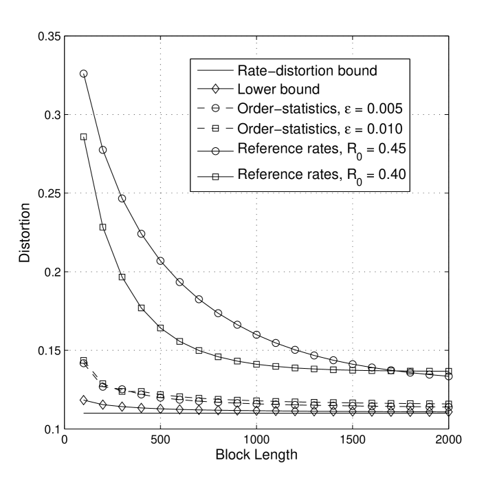
Figure 1: Distortion for the Binary Symmetric Source with Quantization Rate $1/2$.

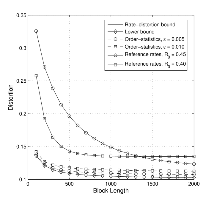
Figure 2: Distortion for the Binary Non-symmetric Source with Distribution $\mathbb{P}(x=1)=0.4$ and Quantization Rate $1/2$.

We consider binary symmetric source with the quantization rate $R=1/2$. The rate distortion theory shows that the lower bound for the distortion for all codeword length is $D^{*}=0.109$. All the numerical computations involved are performed in the log domain, e.g., $2^{1000}$ is represented by $\ln 2^{1000}=1000\ln 2$. For finite quantization block length, we plot distortion lower bound and upper bounds, as well as the asymptotic distortion $0.109$, in Fig. 2. Note that the upper bound based on ordered statistics are plotted for $\epsilon=0.005$ and $0.010$, and the upper bound based on the reference rate are plotted for $R_{0}=0.40$ and $0.45$. It is seen that the upper bound based on ordered statistics becomes tighter for small $\epsilon$; and for upper bound based on the reference rate, smaller $R_{0}$ causes faster attenuation from the beginning but larger converged values, and larger $R_{0}$ causes slower attenuation from the beginning but smaller converged values.

VI Binary Non-symmetric Sources

Consider the length-$n$ independent and identically distributed binary source with non-uniform distribution, with the probability $p$ for bit one and $1-p$ for bit zero, where the probability for a length $n$ sequence with $k$ bits one and $n-k$ bits zero is $p^{k}(1-p)^{n-k}$. Without loss of generality, assume $p\leq 0.5$. Assume that the quantization alphabet size $Q=2^{nR}$. The optimal quantization conditional probability function from the rate-distortion theory is given as follows,

$$\hat{q}(x|y)=\left\{\begin{array}[]{ccc}D&&\mbox{for}\ y\neq x;\\ 1-D&&\mbox{for}\ y=x;\end{array}\right.$$ (156)

for the distortion $D$, $0<D<p$. Then, the probability of $y$ is given by,

$$\mathbb{P}(y=1)=\frac{p-D}{1-2D},\ \ \mbox{and}\ \ \mathbb{P}(y=0)=1-\mathbb{P}(y=1).$$ (157)

The rate-distortion function is given by,

$$R(D)=H(p)-H(D)$$ (158)

for $0\leq D\leq p$ and $R(D)=0$ otherwise.

VI-A Lower Bound

According to Corollary 3, for any quantization using a codebook ${\cal Y}_{Q}=\{{\mbox{\boldmath$y$}}_{1},{\mbox{\boldmath$y$}}_{2},...,{\mbox{\boldmath$y$}}_{Q}\}$ and quantization region ${\cal R}_{j}$ for ${\mbox{\boldmath$y$}}_{j}$ for $1\leq j\leq Q$, the distortion is given by

$$D^{n}(q_{Q})=D^{*}+\frac{\hat{\lambda}}{n}\Big{(}nR-\sum^{Q}_{j=1}\sum_{{\mbox{\boldmath$x$}}\in{\cal R}_{j}}p({\mbox{\boldmath$x$}})\log\frac{\hat{q}({\mbox{\boldmath$x$}}|{\mbox{\boldmath$y$}}_{j})}{p({\mbox{\boldmath$x$}})}\Big{)},$$ (159)

where $\hat{\lambda}=\log_{2}((1-D)/D)$. Note that

$$\sum^{Q}_{j=1}\sum_{{\mbox{\boldmath$x$}}\in{\cal R}_{j}}p({\mbox{\boldmath$x$}})\log\frac{\hat{q}({\mbox{\boldmath$x$}}|{\mbox{\boldmath$y$}}_{j})}{p({\mbox{\boldmath$x$}})} = \sum^{Q}_{j=1}\sum_{{\mbox{\boldmath$x$}}\in{\cal R}_{j}}p({\mbox{\boldmath$x$}})\log\hat{q}({\mbox{\boldmath$x$}}|{\mbox{\boldmath$y$}}_{j})+\sum_{{\mbox{\boldmath$x$}}}p({\mbox{\boldmath$x$}})\log_{2}\frac{1}{p({\mbox{\boldmath$x$}})}$$ (160)

$$= \sum^{Q}_{j=1}\sum_{{\mbox{\boldmath$x$}}\in{\cal R}_{j}}p({\mbox{\boldmath$x$}})\log\hat{q}({\mbox{\boldmath$x$}}|{\mbox{\boldmath$y$}}_{j})+nH(p).$$

We are interested in an upper bound for $\sum^{Q}_{j=1}\sum_{{\mbox{\boldmath$x$}}\in{\cal R}_{j}}p({\mbox{\boldmath$x$}})\log\hat{q}({\mbox{\boldmath$x$}}|{\mbox{\boldmath$y$}}_{j})$. The following result provides an upper bound for the sum of the product of two arrays.

Theorem 24

Assume two arrays $\{a_{i}\}^{N}_{i=1}$ and $\{b_{i}\}^{N}_{i=1}$ satisfy $a_{1}\geq a_{2}...\geq a_{N}\geq 0$ and $b_{1}\geq b_{2}...\geq b_{N}$. Then for any permutation $j_{1}$, $j_{2}$, …, $j_{N}$ of $1$, $2$, …, $N$, we have

$$\sum^{N}_{i=1}a_{i}b_{j_{i}}\leq\sum^{N}_{i=1}a_{i}b_{i}.$$ (161)

According to Theorem 24, we can obtain an upper bound for $\sum^{Q}_{j=1}\sum_{{\mbox{\boldmath$x$}}\in{\cal R}_{j}}p({\mbox{\boldmath$x$}})\log\hat{q}({\mbox{\boldmath$x$}}|{\mbox{\boldmath$y$}}_{j})$ via ranking the two arrays, $\{p({\mbox{\boldmath$x$}}),{\mbox{\boldmath$x$}}\in{\cal X}^{n}\}$ and $\bigcup^{Q}_{j=1}\{\log\hat{q}({\mbox{\boldmath$x$}}|{\mbox{\boldmath$y$}}_{j}),{\mbox{\boldmath$x$}}\in{\cal R}_{j}\}$. Although the latter depends on the selection of the quantization regions ${\cal R}_{j}$, we can further provide an upper bound on $\bigcup^{Q}_{j=1}\{\log\hat{q}({\mbox{\boldmath$x$}}|{\mbox{\boldmath$y$}}_{j}),{\mbox{\boldmath$x$}}\in{\cal R}_{j}\}$ that is independent of ${\cal R}_{j}$.

More specifically, for Hamming distance $H({\mbox{\boldmath$x$}},{\mbox{\boldmath$y$}}_{j})=i$ we have,

$$\log\hat{q}({\mbox{\boldmath$x$}}|{\mbox{\boldmath$y$}}_{j})=i\log D+(n-i)\log(1-D)\stackrel{{\scriptstyle\triangle}}{{=}}d_{i}.$$ (162)

which is independent of ${\mbox{\boldmath$y$}}_{j}$. Then, we can grab the largest $Q=2^{nR}$ values of $\log\hat{q}({\mbox{\boldmath$x$}}|{\mbox{\boldmath$y$}}_{j})$ via finding the distance threshold $D_{T}$ as follows,

$$D_{T}=\max\{D|Q\sum^{D-1}_{j=0}{n\choose j}\leq 2^{n}\},$$

and $$0\leq K<{n\choose D} Q\sum^{D-1}_{j=0}{n\choose j}+K=2^{n}.$$ such that (163)

Let $\{b_{i}\}^{2^{n}}_{i=1}$ denote the array consisting of $Q\cdot{n\choose j}$ elements of $d_{j}$ for $1\leq j\leq D-1$ and $K$ elements of $d_{D}$, in descending order; and let $\{a_{i}\}^{2^{n}}_{i=1}$ denote the $2^{n}$ elements of $p({\mbox{\boldmath$x$}})$ for all ${\mbox{\boldmath$x$}}\in{\cal X}^{n}$, also in descending order. Then we have the following result.

Theorem 25

We have

$$\sum^{Q}_{j=1}\sum_{{\mbox{\boldmath$x$}}\in{\cal R}_{j}}p({\mbox{\boldmath$x$}})\log\hat{q}({\mbox{\boldmath$x$}}|{\mbox{\boldmath$y$}}_{j})\leq\sum^{2^{n}}_{i=1}a_{i}b_{i}.$$ (164)

Furthermore, we have

$$\sum^{2^{n}}_{i=1}a_{i}b_{i}+nH(p)\leq nR,$$ (165)

such that the lower bound obtained from (164) is tighter than the infinite-length distortion $D^{*}$.

Proof:

We rank $\{\log\hat{q}({\mbox{\boldmath$x$}}|{\mbox{\boldmath$y$}}_{j}),{\mbox{\boldmath$x$}}\in{\cal R}_{j},1\leq j\leq Q\}$ in descending order, denoted as $c_{1}\geq c_{2}...\geq c_{2^{n}}$. Since $b_{i}$ is the largest $2^{n}$ values of $\{\log\hat{q}({\mbox{\boldmath$x$}}|{\mbox{\boldmath$y$}}_{j})\}$, we have that $c_{i}\leq b_{i}$ for $1\leq i\leq 2^{n}$, and thus

$$\sum^{Q}_{j=1}\sum_{{\mbox{\boldmath$x$}}\in{\cal R}_{j}}p({\mbox{\boldmath$x$}})\log\hat{q}({\mbox{\boldmath$x$}}|{\mbox{\boldmath$y$}}_{j})\leq\sum^{2^{n}}_{i=1}a_{i}c_{i}\leq\sum^{2^{n}}_{i=1}a_{i}b_{i}.$$ (166)

To prove (165), let $\bar{B}=\sum^{2^{n}}_{i=1}2^{b_{i}}\leq Q=2^{nR}$, and $\tilde{b}_{i}=2^{b_{i}}/\bar{B}$ such that $\sum^{2^{n}}_{i=1}\tilde{b}_{i}=1$. We have that

$$\sum^{2^{n}}_{i=1}a_{i}b_{i}+nH(p) = \sum^{2^{n}}_{i=1}a_{i}\log\frac{\tilde{b}_{i}}{a_{i}}+\sum^{2^{n}}_{i=1}a_{i}\log\bar{B}$$ (167)

$$\leq \frac{1}{\ln 2}\sum^{2^{n}}_{i=1}a_{i}\Big{(}\frac{\tilde{b}_{i}}{a_{i}}-1\Big{)}+\sum^{2^{n}}_{i=1}a_{i}\log\bar{B}$$

$$= \sum^{2^{n}}_{i=1}a_{i}\log\bar{B}=\log\bar{B}\leq nR.$$

∎

Remark: We discuss the computational issues for (164). Note that there are $n+1$ and $D_{T}+1$ different values for $a_{i}$ and $b_{i}$. Then, for $\sum^{2^{n}}_{i=1}a_{i}b_{i}$ all in the descending order, actually there are at most $n+D_{T}+1$ different values of $a_{i}b_{i}$. Computing $\sum^{2^{n}}_{i=1}a_{i}b_{i}$ is to compute the sum of the product of the $n+D_{T}+1$ different values and their frequencies. Here we also compute the sum and product operations in the logarithm domain.

VI-B Upper Bound

We consider the following mean distortion over the codebook

$$\bar{D}_{Q} = \sum_{{\cal Y}_{Q}}p({\cal Y}_{Q})\sum_{{\mbox{\boldmath$x$}}}p({\mbox{\boldmath$x$}})d({\mbox{\boldmath$x$}},{\cal Y}_{Q})=\sum_{{\mbox{\boldmath$x$}}}p({\mbox{\boldmath$x$}})\sum_{{\cal Y}_{Q}}p({\cal Y}_{Q})d({\mbox{\boldmath$x$}},{\cal Y}_{Q})$$ (168)

$$\stackrel{{\scriptstyle\triangle}}{{=}} \sum_{{\mbox{\boldmath$x$}}}p({\mbox{\boldmath$x$}})h_{Q}({\mbox{\boldmath$x$}}).$$

Note that, due to the symmetricity of $x$ for a given weight of $x$, $h_{Q}({\mbox{\boldmath$x$}})$ only depends on the weight of $x$. We derive an upper bound for each weight of $x$. We let $z\stackrel{{\scriptstyle\triangle}}{{=}}\mathbb{P}(y=1)=\frac{p-D}{1-2D}$.

VI-B1 Upper Bound based on Ordered Statistics

Note that for $x$ with weight $w$, we can split it into two parts, $w$ bits one and $n-w$ bits zero. The following result shows the probability $\mathbb{P}\Big{(}d({\mbox{\boldmath$x$}},{\mbox{\boldmath$y$}})=d\Big{)}$ for $x$ with weight $w$. The proof numerates all combinations of the different numbers of bits $i$ and $j$ among the $w$ bits one and $n-w$ bits zero of $x$, respectively.

Theorem 26

For $x$ with weight $w$, we have the following probability

$$\mathbb{P}\Big{(}d({\mbox{\boldmath$x$}},{\mbox{\boldmath$y$}})=d\Big{)}=\sum_{i+j=d,0\leq i\leq w,0\leq j\leq n-w}{w\choose i}z^{w-i}(1-z)^{i}{n-w\choose j}z^{j}(1-z)^{n-w-j}.$$ (169)

Similar to Theorem 22, we have the following result on the upper bound based on ordered statistics.

Theorem 27

For any $\epsilon>0$, we define the threshold $t_{\mbox{\boldmath$x$}}$ as follows,

$$\sum^{t_{\mbox{\boldmath$x$}}-1}_{j=0}\mathbb{P}\Big{(}d({\mbox{\boldmath$x$}},{\mbox{\boldmath$y$}})=j\Big{)}<\frac{\ln\frac{1}{\epsilon}}{Q-1}\leq\sum^{t_{\mbox{\boldmath$x$}}}_{j=0}\mathbb{P}\Big{(}d({\mbox{\boldmath$x$}},{\mbox{\boldmath$y$}})=j\Big{)}.$$ (170)

1. For weight-$w$ sequence $x$, we have the following upper bound

   $$\sum_{{\cal Y}_{Q}}p({\cal Y}_{Q})d({\mbox{\boldmath$x$}},{\cal Y}_{Q})\leq\frac{(1-\epsilon)t_{\mbox{\boldmath$x$}}}{n}+\frac{\epsilon}{2}\stackrel{{\scriptstyle\triangle}}{{=}}D_{w}.$$ (171)

2. Then the upper bound for the distortion $\bar{D}_{Q}$ is given as follows,

   $$\bar{D}_{Q}\leq\sum^{n}_{w=0}{n\choose w}p^{w}(1-p)^{n-w}D_{w}.$$ (172)

VI-B2 Upper Bound based on Reference Rates

Similarly to Theorem 23, we consider a larger distortion $D_{0}>D$ such that the optimal transfer function $\hat{q}(x|y)=D_{0}$ for $y\neq x$ and the corresponding probability $\mathbb{P}(y=1)=\frac{p-D_{0}}{1-2D_{0}}\stackrel{{\scriptstyle\triangle}}{{=}}z_{0}$. We have the following result for the upper bound based on the reference rates for binary non-symmetric source.

Theorem 28

We consider a random codebook where each bit of codeword $y$ satisfies the i.i.d. distribution $\mathbb{P}(y=1)$.

1. For weight $w$ sequence $x$, we have

   $$l({\mbox{\boldmath$x$}},{\mbox{\boldmath$y$}}) \stackrel{{\scriptstyle\triangle}}{{=}} \sum_{{\cal Y}_{Q}}p({\cal Y}_{Q})\Big{(}d({\mbox{\boldmath$x$}},{\cal Y}_{Q})-d({\mbox{\boldmath$x$}},{\mbox{\boldmath$y$}})\Big{)}\Phi({\mbox{\boldmath$x$}},{\mbox{\boldmath$y$}},{\cal Y}_{Q})$$ (173)

   $$\leq z_{0}(1-\frac{w}{n})+(1-z_{0})\frac{w}{n}\stackrel{{\scriptstyle\triangle}}{{=}}u_{w}.$$

2. For weight $w$ sequence $x$, we have

   $$\tilde{h}({\mbox{\boldmath$x$}})=\sum_{{\mbox{\boldmath$y$}}_{0}}\hat{q}({\mbox{\boldmath$y$}}_{0})l({\mbox{\boldmath$x$}},{\mbox{\boldmath$y$}}_{0})\leq u_{w}\frac{1}{Q}\Big{(}\frac{Q-1}{Q}\Big{)}^{Q-1}\stackrel{{\scriptstyle\triangle}}{{=}}\tilde{B}_{w}.$$ (174)

3. For the weight $w$ sequence $x$, we consider the distance threshold $d_{\mbox{\boldmath$x$}}$ and a fraction $0\leq l<1$ such that

   $$\sum^{d_{\mbox{\boldmath$x$}}-1}_{j=0}\mathbb{P}\Big{(}d({\mbox{\boldmath$x$}},{\mbox{\boldmath$y$}})=j\Big{)}\leq\frac{1}{Q}\Big{(}\frac{Q-1}{Q}\Big{)}^{Q-1}<\sum^{d_{\mbox{\boldmath$x$}}}_{j=0}\mathbb{P}\Big{(}d({\mbox{\boldmath$x$}},{\mbox{\boldmath$y$}})=j\Big{)};$$

   and $$\sum^{d_{\mbox{\boldmath$x$}}-1}_{j=0}\mathbb{P}\Big{(}d({\mbox{\boldmath$x$}},{\mbox{\boldmath$y$}})=j\Big{)}+l\cdot\mathbb{P}\Big{(}d({\mbox{\boldmath$x$}},{\mbox{\boldmath$y$}})=d_{\mbox{\boldmath$x$}}\Big{)}=\frac{1}{Q}\Big{(}\frac{Q-1}{Q}\Big{)}^{Q-1}.$$ (175)

   The distortion with respect to $x$ is given as follows,

   $$\tilde{h}({\mbox{\boldmath$x$}}) \leq \sum^{d_{\mbox{\boldmath$x$}}-1}_{j=0}\mathbb{P}\Big{(}d({\mbox{\boldmath$x$}},{\mbox{\boldmath$y$}})=j\Big{)}\frac{D^{j}_{0}(1-D_{0})^{n-j}}{p^{w}(1-p)^{n-w}}+l\cdot\mathbb{P}\Big{(}d({\mbox{\boldmath$x$}},{\mbox{\boldmath$y$}})=d_{\mbox{\boldmath$x$}}\Big{)}\frac{D^{d_{\mbox{\boldmath$x$}}}_{0}(1-D_{0})^{n-d_{\mbox{\boldmath$x$}}}}{p^{w}(1-p)^{n-w}}$$ (176)

   $$\stackrel{{\scriptstyle\triangle}}{{=}} \tilde{h}^{U}_{w},$$

   where the probability $\mathbb{P}\Big{(}d({\mbox{\boldmath$x$}},{\mbox{\boldmath$y$}})=j\Big{)}$ is given by (169). Then, we have,

   $$\bar{D}_{Q}\leq D_{0}+\sum^{n}_{w=0}{n\choose w}p^{w}(1-p)^{n-w}\tilde{h}^{U}_{w}.$$ (177)

Proof:

1. We have the following

   $$l({\mbox{\boldmath$x$}},{\mbox{\boldmath$y$}}) = \sum_{{\cal Y}_{Q}}p({\cal Y}_{Q})\Big{(}d({\mbox{\boldmath$x$}},{\cal Y}_{Q})-d({\mbox{\boldmath$x$}},{\mbox{\boldmath$y$}})\Big{)}\Phi({\mbox{\boldmath$x$}},{\mbox{\boldmath$y$}},{\cal Y}_{Q})$$ (178)

   $$\leq \sum_{{\cal Y}_{Q}}p({\cal Y}_{Q})d({\mbox{\boldmath$x$}},{\cal Y}_{Q})\Phi({\mbox{\boldmath$x$}},{\mbox{\boldmath$y$}},{\cal Y}_{Q})\leq\sum_{{\cal Y}_{Q}}p({\cal Y}_{Q})d({\mbox{\boldmath$x$}},{\cal Y}_{Q})$$

   $$\leq \sum_{{\cal Y}_{Q}}p({\cal Y}_{Q})d({\mbox{\boldmath$x$}},{\mbox{\boldmath$y$}}_{1})=\sum_{{\mbox{\boldmath$y$}}_{1}}p({\mbox{\boldmath$y$}}_{1})d({\mbox{\boldmath$x$}},{\mbox{\boldmath$y$}}_{1})=\mathbb{E}\Big{(}d({\mbox{\boldmath$x$}},{\mbox{\boldmath$y$}}_{1})\big{)}$$

   $$\leq z_{0}(1-\frac{w}{n})+(1-z_{0})\frac{w}{n}\stackrel{{\scriptstyle\triangle}}{{=}}u_{w}.$$

2. The proof is similar to that of Theorems 16 and 17 and thus omitted here.

3. The proof is follows the steps in Theorem 19. We need to note that

   $$p({\mbox{\boldmath$y$}}|{\mbox{\boldmath$x$}})=p({\mbox{\boldmath$y$}})\frac{p({\mbox{\boldmath$x$}}|{\mbox{\boldmath$y$}})}{p({\mbox{\boldmath$x$}})}=\mathbb{P}\Big{(}d({\mbox{\boldmath$x$}},{\mbox{\boldmath$y$}})=j\Big{)}\frac{D^{j}_{0}(1-D_{0})^{n-j}}{p^{w}(1-p)^{n-w}}.$$ (179)

∎

VI-C Numerical Results

We consider binary source with the probability that $\mathbb{P}(x=1)=0.4$, and the quantization rate $R=1/2$. The rate distortion theory shows that the lower bound for the distortion for all codeword length is $D^{*}=0.101$. We show the lower bound, the upper bound from ordered statistics for parameters $\epsilon=0.005$ and $0.010$, and the upper bound from reference rates for parameters $R_{0}=0.45$ and $0.40$. Again, it is seen that the upper bound based on ordered statistics becomes tighter for small $\epsilon$; and for upper bound based on the reference rate, smaller $R_{0}$ causes faster attenuation from the beginning but larger converged values, and larger $R_{0}$ causes slower attenuation from the beginning but smaller converged values.

VII Gaussian Sources

We consider $n$-dimension Gaussian source with the following probability density function

$$p({\mbox{\boldmath$x$}})=\frac{1}{(2\pi\sigma^{2})^{\frac{n}{2}}}e^{-\frac{\|{\mbox{\boldmath$x$}}\|^{2}}{2\sigma^{2}}}.$$ (180)

The distortion measured by the norm-$2$ distortion $d({\mbox{\boldmath$x$}},{\mbox{\boldmath$y$}})=\frac{\|{\mbox{\boldmath$x$}}-{\mbox{\boldmath$y$}}\|^{2}}{n}$. We employ a size-$Q$ codebook, where $Q=2^{nR}$. From the rate-distortion theory, as the dimension $n$ approaches infinity, the quantization distortion approaches to $D$, which satisfies

$$\frac{1}{2}\log_{2}\frac{\sigma^{2}}{D}=R;$$ (181)

and the asymptotic random reconstruction function $\hat{q}({\mbox{\boldmath$x$}}|{\mbox{\boldmath$y$}})$ and $\hat{q}({\mbox{\boldmath$y$}})$ is given as follows,

$$\hat{q}({\mbox{\boldmath$x$}}|{\mbox{\boldmath$y$}})=\frac{1}{(2\pi D)^{\frac{n}{2}}}e^{-\frac{\|{\mbox{\boldmath$x$}}-{\mbox{\boldmath$y$}}\|^{2}}{2D}},\ \mbox{and}\ \ \hat{q}({\mbox{\boldmath$y$}})=\frac{1}{(2\pi(\sigma^{2}-D))^{\frac{n}{2}}}e^{-\frac{\|{\mbox{\boldmath$y$}}\|^{2}}{2(\sigma^{2}-D)}}.$$ (182)

In this Section we derive lower and upper bounds for the optimal quantization distortion using a size-$Q$ codebook. More specifically, we consider the following two cases for the codebook ${\cal Y}_{Q}$,

• bounded codebook: all codewords are constrained within the ball $\|{\mbox{\boldmath$y$}}\|\leq R_{m}$, i.e., $\|{\mbox{\boldmath$y$}}_{j}\|\leq R_{m}$ for all $1\leq j\leq Q$;

• unbounded codebook: all codewords can be chosen from the entire $n$-dimensional real space $\mathbb{R}^{n}$.

VII-A Lower Bound for the Quantization Distortion

From (39), we have that

$$G({\mbox{\boldmath$x$}})=\min_{1\leq j\leq Q}\Big{\{}\frac{\|{\mbox{\boldmath$x$}}-{\mbox{\boldmath$y$}}_{j}\|^{2}}{2D}-\frac{\|{\mbox{\boldmath$x$}}\|^{2}}{2\sigma^{2}}\Big{\}}=\min_{1\leq j\leq Q}G_{j}({\mbox{\boldmath$x$}}),$$ (183)

where $G_{j}({\mbox{\boldmath$x$}})=\frac{\|{\mbox{\boldmath$x$}}-{\mbox{\boldmath$y$}}_{j}\|^{2}}{2D}-\frac{\|{\mbox{\boldmath$x$}}\|^{2}}{2\sigma^{2}}$. We derive a lower bound on the distortion gap $\Delta D^{n}(q_{Q})$ based on Theorem 5 in Section III-C, which provides the following lower bound

$$\Delta D^{n}(q_{Q})\geq\int^{+\infty}_{0}\mathbb{P}\Big{(}G({\mbox{\boldmath$x$}})-1+e^{-G({\mbox{\boldmath$x$}})}\geq\mu\Big{)}d\mu\stackrel{{\scriptstyle\triangle}}{{=}}\Delta\tilde{D}^{n}.$$ (184)

To efficiently derive a lower bound for $\Delta\tilde{D}$ over all possible codebooks ${\cal Y}_{Q}$, i.e., $\min_{{\cal Y}_{Q}}\Delta\tilde{D}$, we add a special codeword ${\mbox{\boldmath$y$}}_{0}\stackrel{{\scriptstyle\triangle}}{{=}}{\bf 0}$ into the codebook. Let $\tilde{\cal Y}_{Q}\stackrel{{\scriptstyle\triangle}}{{=}}{\cal Y}_{Q}\cup\{{\mbox{\boldmath$y$}}_{0}\}$ be the new codebook, and

$$\tilde{G}({\mbox{\boldmath$x$}})\stackrel{{\scriptstyle\triangle}}{{=}}\min_{0\leq j\leq Q}\Big{\{}\frac{\|{\mbox{\boldmath$x$}}-{\mbox{\boldmath$y$}}_{j}\|^{2}}{2D}-\frac{\|{\mbox{\boldmath$x$}}\|^{2}}{2\sigma^{2}}\Big{\}}\leq G({\mbox{\boldmath$x$}}).$$ (185)

Moreover, we define function $E(\mu)$ as the inverse of the function $t-1+e^{-t}$ as follows,

$$E(\mu)=t\ \Leftrightarrow\mu=t-1+e^{-t}\ \mbox{and}\ t\geq 0.$$ (186)

Then, for $t\geq E(\mu)$, we have $t-1+e^{-t}\geq\mu$. We have the following result for a lower bound for $\Delta\tilde{D}$.

Theorem 29

We have the following the lower bound,

$$\Delta\tilde{D}\geq\int^{+\infty}_{0}\mathbb{P}\Big{(}\tilde{G}({\mbox{\boldmath$x$}})\geq E(\mu)\Big{)}d\mu.$$ (187)

Proof:

Note that, due to (185), for $\tilde{G}({\mbox{\boldmath$x$}})\geq E(\mu)$ we have $G({\mbox{\boldmath$x$}})\geq\tilde{G}({\mbox{\boldmath$x$}})\geq E(\mu)$, and thus $G({\mbox{\boldmath$x$}})-1+e^{-G({\mbox{\boldmath$x$}})}\geq\mu$. Therefore

$$\mathbb{P}\Big{(}G({\mbox{\boldmath$x$}})-1+e^{-G({\mbox{\boldmath$x$}})}\geq\mu\Big{)}\geq\mathbb{P}\Big{(}\tilde{G}({\mbox{\boldmath$x$}})\geq E(\mu)\Big{)}.$$ (188)

Via integrating (188) for $\mu$ from $0$ to $+\infty$, we can prove (187). ∎

Based on Theorem 29, in the following we evaluate the lower bound on $\Delta\tilde{D}$ via evaluating an upper bound on $\mathbb{P}\Big{(}\tilde{G}({\mbox{\boldmath$x$}})\leq E(\mu)\Big{)}=1-\mathbb{P}\Big{(}\tilde{G}({\mbox{\boldmath$x$}})\geq E(\mu)\Big{)}$.

VII-A1 Modified Union Bound for $\mathbb{P}\Big{(}\tilde{G}({\mbox{\boldmath$x$}})\leq t\Big{)}$

Here we again let $t=E(\mu)$. Let ${\cal C}_{j}(t)\stackrel{{\scriptstyle\triangle}}{{=}}\{{\mbox{\boldmath$x$}}:G_{j}({\mbox{\boldmath$x$}})\leq t\}$ for $0\leq j\leq Q$. Via simple calculation, we have

$${\mbox{\boldmath$x$}}\in{\cal C}_{j}(t)\Leftrightarrow\|{\mbox{\boldmath$x$}}-\frac{\sigma^{2}}{\sigma^{2}-D}{\mbox{\boldmath$y$}}_{j}\|^{2}\leq\frac{\sigma^{2}D\|{\mbox{\boldmath$y$}}_{j}\|^{2}}{(\sigma^{2}-D)^{2}}+\frac{2D\sigma^{2}t}{\sigma^{2}-D}\stackrel{{\scriptstyle\triangle}}{{=}}R(t,\|{\mbox{\boldmath$y$}}_{j}\|),\ 0\leq j\leq Q;$$ (189)

and in particular

$${\mbox{\boldmath$x$}}\in{\cal C}_{0}(t)\Leftrightarrow\|{\mbox{\boldmath$x$}}\|^{2}\leq\frac{2D\sigma^{2}t}{\sigma^{2}-D}=R(t,0).$$ (190)

According to (189), for each $0\leq j\leq Q$, ${\cal C}_{j}(t)$ is a ball with center $\frac{\sigma^{2}}{\sigma^{2}-D}{\mbox{\boldmath$y$}}_{j}$ and radius $\sqrt{R(t,\|{\mbox{\boldmath$y$}}_{j}\|^{2})}$.

We have the following modified union bound for $\mathbb{P}\Big{(}\tilde{G}({\mbox{\boldmath$x$}})\leq t\Big{)}$.

Theorem 30

We have the following upper bound for $\mathbb{P}\Big{(}\tilde{G}({\mbox{\boldmath$x$}})\leq t\Big{)}$,

$$\mathbb{P}\Big{(}\tilde{G}({\mbox{\boldmath$x$}})\leq t\Big{)}\leq\mathbb{P}\Big{(}{\cal C}_{0}(t)\Big{)}+\sum^{Q}_{j=1}\mathbb{P}\Big{(}{\cal C}_{j}(t)\setminus{\cal C}_{0}(t)\Big{)}.$$ (191)

Proof:

Note that

$$G({\mbox{\boldmath$x$}})=\min_{0\leq j\leq Q}G_{j}({\mbox{\boldmath$x$}})\leq t\Leftrightarrow{\mbox{\boldmath$x$}}\in\cup^{Q}_{j=0}{\cal C}_{j}(t);$$ (192)

and $\cup^{Q}_{j=0}{\cal C}_{j}(t)={\cal C}_{0}(t)\cup\cup^{Q}_{j=1}\Big{(}{\cal C}_{j}(t)\setminus{\cal C}_{0}(t)\Big{)}$. Then, we have

$$\mathbb{P}\Big{(}G({\mbox{\boldmath$x$}})\leq t\Big{)}=\mathbb{P}\Big{(}\cup^{Q}_{j=0}{\cal C}_{j}(t)\Big{)}\leq\mathbb{P}\Big{(}{\cal C}_{0}(t)\Big{)}+\sum^{Q}_{j=1}\mathbb{P}\Big{(}{\cal C}_{j}(t)\setminus{\cal C}_{0}(t)\Big{)}.$$ (193)

∎

Note that ${\cal C}_{j}(t)\setminus{\cal C}_{0}(t)$ denotes the space in the ball ${\cal C}_{j}(t)$ but not in ${\cal C}_{0}(t)$. Due to the sphere symmetric property of Gaussian distribution, $\mathbb{P}\Big{(}{\cal C}_{j}(t)\setminus{\cal C}_{0}(t)\Big{)}$ is only a function of $\|{\mbox{\boldmath$y$}}_{j}\|$, and $t$. Based on the computational methods in Section IX-B, we have the following result on the probability $\mathbb{P}\Big{(}{\cal C}_{j}(t)\setminus{\cal C}_{0}(t)\Big{)}$.

Theorem 31

Let

$$r_{min} = \max\Big{\{}\sqrt{R(t,0)},\frac{\sigma^{2}}{\sigma^{2}-D}\|{\mbox{\boldmath$y$}}_{j}\|-\sqrt{R(t,\|{\mbox{\boldmath$y$}}_{j}\|)}\Big{\}},$$

$$r_{max} = \frac{\sigma^{2}}{\sigma^{2}-D}\|{\mbox{\boldmath$y$}}_{j}\|+\sqrt{R(t,\|{\mbox{\boldmath$y$}}_{j}\|)}.$$ (194)

The probability $\mathbb{P}\Big{(}{\cal C}_{j}(t)\setminus{\cal C}_{0}(t)\Big{)}$ is given as follows,

$$\mathbb{P}\Big{(}{\cal C}_{j}(t)\setminus{\cal C}_{0}(t)\Big{)}=\int^{r_{max}}_{r_{min}}\frac{1}{(2\pi\sigma^{2})^{\frac{n}{2}}}e^{-\frac{r^{2}}{2\sigma^{2}}}r^{n-1}\Omega_{n}(\theta_{j}(r))dr,$$ (195)

where the semiangle $\theta_{j}(r)$ is given as follows,

$$\theta_{j}(r)=\cos^{-1}\frac{\Big{(}\frac{\sigma^{2}}{\sigma^{2}-D}\Big{)}^{2}\|{\mbox{\boldmath$y$}}_{j}\|^{2}+r^{2}-R(t,\|{\mbox{\boldmath$y$}}_{j}\|)}{2\frac{\sigma^{2}}{\sigma^{2}-D}\|{\mbox{\boldmath$y$}}_{j}\|r}.$$ (196)

Proof:

Consider the intersection of ${\cal C}_{j}(t)\setminus{\cal C}_{0}(t)$ with a radius-$r$ sphere centered at the origin, which is essentially a radius-$r$ sphere cut out by a cone. The cone can be described by a triangular with the lengths $\Big{(}\frac{\sigma^{2}}{\sigma^{2}-D}\|{\mbox{\boldmath$y$}}_{j}\|,r,\sqrt{R(\|{\mbox{\boldmath$y$}}_{j}\|^{2},t)}\Big{)}$ of the three edges; and the semiangle is the angle between the edges of lengths $\frac{\sigma^{2}}{\sigma^{2}-D}\|{\mbox{\boldmath$y$}}_{j}\|$ and $r$. Then, from the cosine formula, we have that

$$\Big{(}\frac{\sigma^{2}}{\sigma^{2}-D}\Big{)}^{2}\|{\mbox{\boldmath$y$}}_{j}\|^{2}+r^{2}-2\frac{\sigma^{2}}{\sigma^{2}-D}\|{\mbox{\boldmath$y$}}_{j}\|r\cos\theta_{j}(r)=R_{j}(t);$$ (197)

and thus (196) follows (197); and the sphere area is given by $r^{n-1}\Omega_{n}(\theta_{j}(r))$.

Next we consider such radius-$r$ sphere that can have non-empty intersection with ${\cal C}_{j}(t)\setminus{\cal C}_{0}(t)$. Note that, if $\sqrt{R(t),0}<\frac{\sigma^{2}}{\sigma^{2}-D}\|{\mbox{\boldmath$y$}}_{j}\|-\sqrt{R(t,\|{\mbox{\boldmath$y$}}_{j}\|)}$, then ${\cal C}_{j}(t)\cap{\cal C}_{0}(t)=\emptyset$ and thus ${\cal C}_{j}(t)\setminus{\cal C}_{0}(t)={\cal C}_{j}(t)$. The range of $r$ is from $\frac{\sigma^{2}}{\sigma^{2}-D}\|{\mbox{\boldmath$y$}}_{j}\|-\sqrt{R(t,\|{\mbox{\boldmath$y$}}_{j}\|)}$ to $r_{max}$ [c.f. (31)]. Otherwise if $\sqrt{R(t,0)}\geq\frac{\sigma^{2}}{\sigma^{2}-D}\|{\mbox{\boldmath$y$}}_{j}\|-\sqrt{R(t,\|{\mbox{\boldmath$y$}}_{j}\|)}$, the range of $r$ is from $\sqrt{R(t,0)}$ to $r_{max}$ [c.f. (31)]. Thus the range of $r$ is from $r_{min}$ to $r_{max}$ as specified by (31).

Finally, via integrating the following probability density of Gaussian distribution on a radius-$r$ sphere,

$$\frac{1}{(2\pi\sigma^{2})^{\frac{n}{2}}}e^{-\frac{r^{2}}{2\sigma^{2}}},$$ (198)

over the intersection with ${\cal C}_{j}(t)\cap{\cal C}_{0}(t)$ with the semiangle $\Omega_{n}(\theta_{j}(r))$, we have the expression of the probability $\mathbb{P}\Big{(}{\cal C}_{j}(t)\setminus{\cal C}_{0}(t)\Big{)}$ as in (195). ∎

$\hfill\Box$

Note that the upper bounds obtained from Theorems 30 and 31 may exceed $1$. In the following we propose another bound upper bound for bounded codeword constraint, i.e., $\|{\mbox{\boldmath$y$}}_{j}\|\leq R_{m}$ for all $1\leq j\leq Q$. More specifically, for each $1\leq j\leq Q$, we consider a codeword ${\mbox{\boldmath$y$}}_{j}$ lying on the boundary $\|{\mbox{\boldmath$y$}}_{j}\|=R_{m}$ with a radius $\sqrt{R(t,R_{m})}$, denoted as $\tilde{\cal C}_{j}(t)$; and for consistency let $\tilde{\cal C}_{0}(t)={\cal C}_{0}(t)$. We compute the an upper bound for the volume of $\cup^{Q}_{j=0}\tilde{\cal C}_{j}(t)$, denoted as ${\cal V}_{n}(\cup^{Q}_{j=0}\tilde{\cal C}_{j}(t))$. The upper bound for the volume ${\cal V}_{n}\Big{(}\cup^{Q}_{j=0}\tilde{\cal C}_{j}(t)\Big{)}$ can be proved to be an upper bound for the volume ${\cal V}_{n}\Big{(}\cup^{Q}_{j=0}{\cal C}_{j}(t)\Big{)}$. The probability $\mathbb{P}\Big{(}\cup^{Q}_{j=0}\tilde{\cal C}_{j}(t)\Big{)}$ is upper bounded by the probability of the ball with the center at zero with the same volume. The following results show that, although the exact value of ${\cal V}_{n}\Big{(}\cup^{Q}_{j=0}\tilde{\cal C}_{j}(t)\Big{)}$ is difficult to compute, we are able to derive an upper bound for ${\cal V}_{n}\Big{(}\cup^{Q}_{j=0}\tilde{\cal C}_{j}(t)\Big{)}$ and the associated upper bound for the probability $\mathbb{P}\Big{(}\cup^{Q}_{j=0}\tilde{\cal C}_{j}(t)\Big{)}$.

Theorem 32

For bounded codewords $\|{\mbox{\boldmath$y$}}_{j}\|\leq R_{m}$ for $1\leq j\leq Q$, an upper for the volume ${\cal V}_{n}\Big{(}\cup^{Q}_{j=0}{\cal C}_{j}(t)\Big{)}$ is given as follows,

$${\cal V}_{n}\Big{(}\cup^{Q}_{j=0}{\cal C}_{j}(t)\Big{)}\leq{\cal V}_{n}\Big{(}\tilde{\cal C}_{0}(t)\Big{)}+\sum^{Q}_{j=1}{\cal V}_{n}\Big{(}\tilde{\cal C}_{j}(t)\setminus{\cal C}_{0}(t)\Big{)}\stackrel{{\scriptstyle\triangle}}{{=}}\tilde{V}_{n}.$$ (199)

Define the radius $r_{n}$ as follows,

$$r_{n}\stackrel{{\scriptstyle\triangle}}{{=}}\Big{(}\frac{\tilde{V}_{n}}{V_{n}}\Big{)}^{\frac{1}{n}},$$ (200)

where $V_{n}$ is the volume of a unit ball in a dimension-$n$ space; and define another radius

$$\tilde{r}_{n}\stackrel{{\scriptstyle\triangle}}{{=}}\frac{\sigma^{2}R_{m}}{\sigma^{2}-D}+\sqrt{R(t,R_{m})}.$$ (201)

Let $r_{E}=\min\{r_{n},\tilde{r}_{n}\}$, an upper bound for the probability $\mathbb{P}\Big{(}\cup^{Q}_{j=0}{\cal C}_{j}(t)\Big{)}$ is given as follows,

$$\mathbb{P}\Big{(}\cup^{Q}_{j=0}{\cal C}_{j}(t)\Big{)}\leq\Upsilon_{n}\Big{(}\frac{r^{2}_{E}}{\sigma^{2}}\Big{)}\stackrel{{\scriptstyle\triangle}}{{=}}\Gamma_{n}(t).$$ (202)

$\hfill\Box$

The following result provides an upper bound on ${\cal V}_{n}\Big{(}\tilde{\cal C}_{j}(t)\setminus{\cal C}_{0}(t)\Big{)}$. The proof is similar to that of Theorem 31, and thus omitted here.

Theorem 33

Given $\|\tilde{\mbox{\boldmath$y$}}_{j}\|=R_{m}$ and the ball $\tilde{\cal C}_{j}(t)$, given by

$$\tilde{\cal C}_{j}(t)=\Big{\{}{\mbox{\boldmath$x$}}:\|{\mbox{\boldmath$x$}}-\frac{\sigma^{2}}{\sigma^{2}-D}\tilde{\mbox{\boldmath$y$}}_{j}\|\leq\sqrt{R(t,R_{m})}\Big{\}}.$$ (203)

Letting

$$\tilde{r}_{min} = \max\Big{\{}\sqrt{R(t,0)},\frac{\sigma^{2}}{\sigma^{2}-D}R_{m}-\sqrt{R(t,R_{m})}\Big{\}},$$

$$\tilde{r}_{max} = \frac{\sigma^{2}}{\sigma^{2}-D}R_{m}+\sqrt{R(t,R_{m})},$$ (204)

we have

$${\cal V}_{n}\Big{(}\tilde{\cal C}_{j}(t)\setminus{\cal C}_{0}(t)\Big{)}=\int^{\tilde{r}_{max}}_{\tilde{r}_{min}}r^{n-1}\Omega_{n}(\tilde{\theta}_{j}(r))dr,$$ (205)

where the semiangle

$$\tilde{\theta}_{j}(r)=\cos^{-1}\frac{\Big{(}\frac{\sigma^{2}}{\sigma^{2}-D}\Big{)}^{2}R_{m}^{2}+r^{2}-R(t,R_{m})}{2\frac{\sigma^{2}}{\sigma^{2}-D}R_{m}r}.$$ (206)

$\hfill\Box$

Note that the above upper bound is for the bounded quantization codewords $\|{\mbox{\boldmath$y$}}_{j}\|\leq R_{m}$. For unbounded quantization codewords, we simply set $\Gamma_{n}(t)=1$. Moreover, the probability $\mathbb{P}\Big{(}{\cal C}_{0}(t)\Big{)}$ is a function of $t$, denoted as $K_{0}(t)$; and the probability $\mathbb{P}\Big{(}{\cal C}_{0}(t)\setminus{\cal C}_{j}(t)\Big{)}$ is a function of $\|{\mbox{\boldmath$y$}}_{j}\|$ and $t$, denoted as $K(t,\|{\mbox{\boldmath$y$}}_{j}\|)$. Thus we can write the upper bound in Theorems 30 and 31 as follows,

$$\mathbb{P}\Big{(}\cup^{Q}_{j=0}{\cal C}_{j}(t)\Big{)}\leq K_{0}(t)+\sum^{Q}_{j=1}K(t,\|{\mbox{\boldmath$y$}}_{j}\|),$$ (207)

where $K_{0}(t)=\mathbb{P}\Big{(}{\cal C}_{0}(t)\Big{)}$. Via combining the results in Theorems 30 to 33, we have the following result on an upper bound for $\mathbb{P}\Big{(}\tilde{G}({\mbox{\boldmath$x$}})\leq t\Big{)}=\mathbb{P}\Big{(}\cup^{Q}_{j=0}{\cal C}_{j}(t)\Big{)}$.

Theorem 34

An upper bound on $\mathbb{P}\Big{(}G({\mbox{\boldmath$x$}})\leq t\Big{)}$ is given as follows,

$$\mathbb{P}\Big{(}G({\mbox{\boldmath$x$}})\leq t\Big{)}=\mathbb{P}\Big{(}\cup^{Q}_{j=0}{\cal C}_{j}(t)\Big{)}\leq\min\Big{\{}K_{0}(t)+\sum^{Q}_{j=1}K(\|{\mbox{\boldmath$y$}}_{j}\|,t),\Gamma(t)\Big{\}}.$$ (208)

$\hfill\Box$

VII-A2 A Lower Bound for $\Delta\tilde{D}$

Via letting $t=E(\mu)$, from (208) we have

$$\mathbb{P}\Big{(}\tilde{G}({\mbox{\boldmath$x$}})\leq E(\mu)\Big{)} \leq \min\Big{\{}K_{0}(E(\mu))+\sum^{Q}_{j=1}K(\|{\mbox{\boldmath$y$}}_{j}\|,E(\mu)),\Gamma(E(\mu))\Big{\}}$$ (209)

$$\stackrel{{\scriptstyle\triangle}}{{=}} \min\Big{\{}\tilde{K}_{0}(\mu)+\sum^{Q}_{j=1}\tilde{K}(\|{\mbox{\boldmath$y$}}_{j}\|,\mu),\tilde{\Gamma}(\mu)\Big{\}}.$$

Then, we have the following lower bound,

$$\Delta\tilde{D}\geq\int^{+\infty}_{0}\Big{(}1-\min\Big{\{}\tilde{K}_{0}(\mu)+\sum^{Q}_{j=1}\tilde{K}(\|{\mbox{\boldmath$y$}}_{j}\|,\mu),\tilde{\Gamma}(\mu)\Big{\}}\Big{)}d\mu\stackrel{{\scriptstyle\triangle}}{{=}}\Delta\hat{D}.$$ (210)

Since the codewords $\{{\mbox{\boldmath$y$}}_{j}\}_{1\leq j\leq Q}$, can be arbitrarily selected, we need to minimize $\hat{D}$ subject to all possible codewords $\{{\mbox{\boldmath$y$}}_{j}\}_{1\leq j\leq Q}$, i.e., to obtain a lower bound of the following,

$$\min_{\{{\mbox{\boldmath$y$}}_{j}\}_{1\leq j\leq Q}}\Delta\hat{D}.$$ (211)

However, directly solving (211) incurs prohibitive computational complexity. The following result provides a further lower bound of $\Delta\hat{D}$, which is significantly more computational feasible.

It is observed that,

$$\tilde{K}_{0}(\mu)+\sum^{Q}_{j=1}\tilde{K}(\|{\mbox{\boldmath$y$}}_{j}\|,\mu)<\tilde{\Gamma}(\mu),$$ (212)

for small $\mu$ and the vice versa for large $\mu$. Based on this observation, we set up a parameter $\mu_{0}\geq 0$, and let

$$\Delta\hat{D}(\mu_{0})\stackrel{{\scriptstyle\triangle}}{{=}}\int^{\mu_{0}}_{0}\Big{(}1-\tilde{K}_{0}(\mu)-\sum^{Q}_{j=1}\tilde{K}(\|{\mbox{\boldmath$y$}}_{j}\|,\mu)\Big{)}d\mu+\int^{+\infty}_{\mu_{0}}\Big{(}1-\tilde{\Gamma}(\mu)\Big{)}d\mu.$$ (213)

It is easily seen that, for any $\{{\mbox{\boldmath$y$}}_{j}\}^{Q}_{j=1}$, we have that $\Delta\hat{D}(\mu_{0})\leq\Delta\hat{D}$. However, since in (213) all ${\mbox{\boldmath$y$}}_{j}$ for $1\leq j\leq Q$ are independent, the lower bound $\min_{\{{\mbox{\boldmath$y$}}_{j}\}_{1\leq j\leq Q}}\Delta\hat{D}(\mu_{0})$ can be solved via solving,

$$\max_{\|{\mbox{\boldmath$y$}}_{j}\|}\int^{\mu_{0}}_{0}\tilde{K}(\|{\mbox{\boldmath$y$}}_{j}\|,\mu)d\mu.$$ (214)

Note that the above optimization problems are the same for all $1\leq j\leq Q$, and we can solve (215) for all ${\mbox{\boldmath$y$}}_{j}$. The following Theorem 35 formalizes the above arguments.

Theorem 35

For any $\mu_{0}\geq 0$, we have that

$$\min_{\{{\mbox{\boldmath$y$}}_{j}\}_{1\leq j\leq Q}}\Delta\hat{D}(\mu_{0})\leq\min_{\{{\mbox{\boldmath$y$}}_{j}\}_{1\leq j\leq Q}}\Delta\hat{D}.$$ (215)

• For bounded codebook constraints $\|{\mbox{\boldmath$y$}}_{j}\|\leq R_{m}$ for $1\leq j\leq Q$, we have

  $$\min_{\{{\mbox{\boldmath$y$}}_{j}\}_{1\leq j\leq Q}}\Delta\hat{D}(\mu_{0}) = \min_{0\leq r\leq R_{m}}\int^{\mu_{0}}_{0}\Big{(}1-\tilde{K}_{0}(\mu)-Q\tilde{K}(r,\mu)\Big{)}d\mu+\int^{+\infty}_{\mu_{0}}\Big{(}1-\tilde{\Gamma}(\mu)\Big{)}d\mu$$ (216)

  $$\stackrel{{\scriptstyle\triangle}}{{=}} \min_{0\leq r\leq R_{m}}\Delta\hat{D}(\mu_{0},r).$$

  Thus, we have

  $$\sup_{\mu_{0}}\min_{0\leq r\leq R_{m}}\Delta\hat{D}(\mu_{0},r)\leq\min_{\{{\mbox{\boldmath$y$}}_{j}\}_{1\leq j\leq Q}}\Delta\hat{D}.$$ (217)

• For unbounded codebook, then $\tilde{\Gamma}(\mu)=1$ for all $\mu\geq 0$, we have

  $$\min_{\{{\mbox{\boldmath$y$}}_{j}\}_{1\leq j\leq Q}}\Delta\hat{D}(\mu_{0}) = \inf_{r\geq 0}\int^{\mu_{0}}_{0}\Big{(}1-\tilde{K}_{0}(\mu)-Q\tilde{K}(r,\mu)\Big{)}d\mu$$ (218)

  $$\stackrel{{\scriptstyle\triangle}}{{=}} \inf_{r\geq 0}\Delta\hat{D}(\mu_{0},r).$$

  Thus we have

  $$\sup_{\mu_{0}\geq 0}\inf_{r\geq 0}\Delta\hat{D}(\mu_{0},r)\leq\min_{\{{\mbox{\boldmath$y$}}_{j}\}_{1\leq j\leq Q}}\Delta\hat{D}.$$ (219)

Proof:

Note that for any $\{{\mbox{\boldmath$y$}}_{j}\}_{1\leq j\leq Q}$ we have $\Delta\hat{D}(\mu_{0})\leq\Delta\hat{D}$. Then, minimizing the left side among all $\{{\mbox{\boldmath$y$}}_{j}\}_{1\leq j\leq Q}$ we have

$$\min_{\{{\mbox{\boldmath$y$}}_{j}\}_{1\leq j\leq Q}}\Delta\hat{D}(\mu_{0})\leq\Delta\hat{D};$$ (220)

and via minimizing the right side among all $\{{\mbox{\boldmath$y$}}_{j}\}_{1\leq j\leq Q}$ we have

$$\min_{\{{\mbox{\boldmath$y$}}_{j}\}_{1\leq j\leq Q}}\Delta\hat{D}(\mu_{0})\leq\min_{\{{\mbox{\boldmath$y$}}_{j}\}_{1\leq j\leq Q}}\Delta\hat{D},$$ (221)

and thus prove (215).

Then, according to (213), we have that

$$\min_{\{{\mbox{\boldmath$y$}}_{j}\}_{1\leq j\leq Q}}\Delta\hat{D}(\mu_{0}) = \int^{\mu_{0}}_{0}\Big{(}1-\tilde{K}_{0}(\mu)\Big{)}d\mu-\sum^{Q}_{j=1}\max_{{\mbox{\boldmath$y$}}_{j}}\int^{\mu_{0}}_{0}\tilde{K}(\|{\mbox{\boldmath$y$}}_{j}\|,\mu)d\mu+\int^{+\infty}_{\mu_{0}}\Big{(}1-\tilde{\Gamma}(\mu)\Big{)}d\mu$$ (222)

$$= \int^{\mu_{0}}_{0}\Big{(}1-\tilde{K}_{0}(\mu)\Big{)}d\mu-Q\max_{0\leq r\leq R_{m}}\int^{\mu_{0}}_{0}\tilde{K}(r,\mu)d\mu+\int^{+\infty}_{\mu_{0}}\Big{(}1-\tilde{\Gamma}(\mu)\Big{)}d\mu$$

$$= \min_{0\leq r\leq R_{m}}\int^{\mu_{0}}_{0}\Big{(}1-\tilde{K}_{0}(\mu)-Q\tilde{K}(r,\mu)\Big{)}d\mu+\int^{+\infty}_{\mu_{0}}\Big{(}1-\tilde{\Gamma}(\mu)\Big{)}d\mu$$

$$= \min_{0\leq r\leq R_{m}}\Delta\hat{D}(\mu_{0},r),$$

and thus prove (216).

Finally, since

$$\min_{0\leq r\leq R_{m}}\Delta\hat{D}(\mu_{0},r)\leq\min_{\{{\mbox{\boldmath$y$}}_{j}\}_{1\leq j\leq Q}}\Delta\hat{D},$$ (223)

for all $\mu_{0}\geq 0$, we can select the supreme of the left side, and thus prove (217). ∎

Remark 3: It is easily seen that for $\mu_{0}=0$, $\Delta\hat{D}(\mu_{0},r)\geq 0$ for all $r\geq 0$. Thus we have

$$\sup_{\mu_{0}\geq 0}\inf_{r\geq 0}\Delta\hat{D}(\mu_{0},r)\geq\inf_{r\geq 0}\Delta\hat{D}(0,r)\geq 0.$$ (224)

Therefore, the lower bound $\sup_{\mu_{0}\geq 0}\inf_{r\geq 0}\Delta\hat{D}(\mu_{0},r)$ is well-defined.

VII-B Upper Bound

Due to the high computational complexity of the upper bound based on the reference rate, we only provide an upper bound based on ordered statistics.

VII-B1 Upper Bound for Unbounded Sources

We derive an upper for Gaussian sources based on Theorem 13. Let ${\mbox{\boldmath$y$}}_{b}={\bf 0}$ and ${\cal B}^{n}_{\delta}=\{{\mbox{\boldmath$x$}}:\|{\mbox{\boldmath$x$}}\|^{2}\leq(1+\delta)\sigma^{2}\}$, such that for all ${\mbox{\boldmath$x$}}\in{\cal B}^{n}_{\delta}$ we have that $d({\mbox{\boldmath$x$}},{\mbox{\boldmath$y$}}_{b})\leq 1+\delta$. In the following we evaluate each term involved in Theorem 13 and specify the upper bound for Gaussian sources.

We evaluate the probability $\mathbb{P}\Big{(}d({\mbox{\boldmath$x$}},{\mbox{\boldmath$y$}})\leq t_{\mbox{\boldmath$x$}}\Big{)}$ based on non-central chi-squared distribution. Note that due to (182), we have that

$$P\Big{(}\|{\mbox{\boldmath$y$}}-{\mbox{\boldmath$x$}}\|^{2}\leq\beta^{2}\Big{)}=\Upsilon_{n}\Big{(}\frac{\beta^{2}}{\sigma^{2}-D},\frac{\|{\mbox{\boldmath$x$}}\|^{2}}{\sigma^{2}-D}\Big{)},$$ (225)

where $\Upsilon_{(}\cdot,\cdot)$ is the non-central chi-squared specified in (245). Since given $x$, $P\Big{(}\|{\mbox{\boldmath$y$}}-{\mbox{\boldmath$x$}}\|^{2}\leq\beta^{2}\Big{)}$ is strictly increasing with $\beta^{2}$, we can define the following inverse function,

$$\frac{\beta^{2}}{\sigma^{2}-D}=\Theta_{n}\Big{(}\frac{\|{\mbox{\boldmath$x$}}\|^{2}}{\sigma^{2}-D},P_{0}\Big{)},$$ (226)

if $P_{0}=P\Big{(}\|{\mbox{\boldmath$y$}}-{\mbox{\boldmath$x$}}\|^{2}\Big{)}$. Moreover, let $\upsilon_{n}(x)$ be the probability density function be the order-$n$ Chi-squared distribution given as follows,

$$\upsilon_{n}(x) = \frac{1}{2^{n/2}\Gamma(n/2)}x^{n/2-1}e^{-x/2},$$ (227)

which is the pdf of the squared sum of $n$ independently unit Gaussian distributed variables. We integrate in the $n$-dimensional space according to that squared sum and have the following result.

Theorem 36

For any $\delta,\epsilon>0$, we have the following upper bound

$$\bar{D}_{Q} \leq \int^{n(\sigma^{2}+\delta)}_{0}\frac{1}{\sigma^{2}}\upsilon_{n}\Big{(}\frac{x}{\sigma^{2}}\Big{)}\min\Big{\{}\frac{x}{n},\frac{(\sigma^{2}-D)}{n}\Theta_{n}\Big{(}\frac{x}{\sigma^{2}-D},\frac{\ln\frac{1}{\epsilon}}{Q-2}\Big{)}\Big{\}}dx$$ (228)

$$\ \ \ +\int^{+\infty}_{n(\sigma^{2}+\delta)}\frac{x}{\sigma^{2}}\upsilon_{n}\Big{(}\frac{x}{\sigma^{2}}\Big{)}dx+\epsilon(2\sigma^{2}-D).$$

Proof:

We analyze each term involved in Theorem 13. First, we have that

$$\int_{\bar{\cal B}^{n}_{\delta}}p({\mbox{\boldmath$x$}})d({\mbox{\boldmath$x$}},{\mbox{\boldmath$y$}}_{b})d{\mbox{\boldmath$x$}} = \int_{\|{\mbox{\boldmath$x$}}\|^{2}\geq n(\sigma^{2}+\delta)}\|{\mbox{\boldmath$x$}}\|^{2}p({\mbox{\boldmath$x$}})d{\mbox{\boldmath$x$}}$$ (229)

$$= \int^{+\infty}_{n(\sigma^{2}+\delta)}\frac{x}{\sigma^{2}}\upsilon_{n}\Big{(}\frac{x}{\sigma^{2}}\Big{)}dx.$$

Then, according to Theorem 13, we have the following

$$\epsilon\int\int p({\mbox{\boldmath$x$}})\hat{q}({\mbox{\boldmath$y$}})d({\mbox{\boldmath$x$}},{\mbox{\boldmath$y$}})d{\mbox{\boldmath$x$}}d{\mbox{\boldmath$y$}}$$ (230)

$$= \epsilon\int\int p({\mbox{\boldmath$x$}})\hat{q}({\mbox{\boldmath$y$}})\frac{\|{\mbox{\boldmath$x$}}-{\mbox{\boldmath$y$}}\|^{2}}{n}d{\mbox{\boldmath$x$}}d{\mbox{\boldmath$y$}}$$

$$= \epsilon\int\int p({\mbox{\boldmath$x$}})\hat{q}({\mbox{\boldmath$y$}})\frac{\|{\mbox{\boldmath$x$}}\|^{2}}{n}d{\mbox{\boldmath$x$}}d{\mbox{\boldmath$y$}}+\epsilon\int\int p({\mbox{\boldmath$x$}})\hat{q}({\mbox{\boldmath$y$}})\frac{\|{\mbox{\boldmath$y$}}\|^{2}}{n}d{\mbox{\boldmath$x$}}d{\mbox{\boldmath$y$}}-\epsilon\int\int p({\mbox{\boldmath$x$}})\hat{q}({\mbox{\boldmath$y$}})\frac{2{\mbox{\boldmath$x$}}^{T}{\mbox{\boldmath$y$}}}{n}d{\mbox{\boldmath$x$}}d{\mbox{\boldmath$y$}}$$

$$= \epsilon\int p({\mbox{\boldmath$x$}})\frac{\|{\mbox{\boldmath$x$}}\|^{2}}{n}d{\mbox{\boldmath$x$}}+\epsilon\int\hat{q}({\mbox{\boldmath$y$}})\frac{\|{\mbox{\boldmath$y$}}\|^{2}}{n}d{\mbox{\boldmath$y$}}$$

$$= \epsilon\sigma^{2}+\epsilon(\sigma^{2}-D)=\epsilon(2\sigma^{2}-D).$$

Finally, given $x$, we have that the radius $t_{\mbox{\boldmath$x$}}$ is given as follows,

$$P\Big{(}\frac{\|{\mbox{\boldmath$y$}}-{\mbox{\boldmath$x$}}\|^{2}}{n}\leq t_{\mbox{\boldmath$x$}}\Big{)}=\Upsilon_{n}\Big{(}\frac{\|{\mbox{\boldmath$x$}}\|^{2}}{\sigma^{2}-D},\frac{nt_{\mbox{\boldmath$x$}}}{\sigma^{2}-D}\Big{)}=1-\epsilon^{\frac{1}{Q-2}}\leq\frac{\ln\frac{1}{\epsilon}}{Q-2},$$ (231)

and thus we have that

$$t_{\mbox{\boldmath$x$}}\leq\frac{(\sigma^{2}-D)}{n}\Theta_{n}\Big{(}\frac{\|{\mbox{\boldmath$x$}}\|^{2}}{\sigma^{2}-D},\frac{\ln\frac{1}{\epsilon}}{Q-2}\Big{)}.$$ (232)

Then, we have the following,

$$\min\Big{\{}d({\mbox{\boldmath$x$}},{\bf 0}),t_{\mbox{\boldmath$x$}}\Big{\}}\leq\min\Big{\{}\frac{\|{\mbox{\boldmath$x$}}\|^{2}}{n},\frac{(\sigma^{2}-D)}{n}\Theta_{n}\Big{(}\frac{\|{\mbox{\boldmath$x$}}\|^{2}}{\sigma^{2}-D},\frac{\ln\frac{1}{\epsilon}}{Q-2}\Big{)}\Big{\}},$$ (233)

and thus

$$\int_{{\cal B}^{n}_{\delta}}p({\mbox{\boldmath$x$}})\min\Big{\{}d({\mbox{\boldmath$x$}},{\bf 0}),t_{\mbox{\boldmath$x$}}\Big{\}}d{\mbox{\boldmath$x$}}$$ (234)

$$\leq \int_{\|{\mbox{\boldmath$x$}}\|^{2}\leq n(\sigma^{2}+\delta)}p({\mbox{\boldmath$x$}})\min\Big{\{}\frac{\|{\mbox{\boldmath$x$}}\|^{2}}{n},\frac{(\sigma^{2}-D)}{n}\Theta_{n}\Big{(}\frac{\|{\mbox{\boldmath$x$}}\|^{2}}{\sigma^{2}-D},\frac{\ln\frac{1}{\epsilon}}{Q-2}\Big{)}\Big{\}}d{\mbox{\boldmath$x$}}$$

$$= \int^{n(\sigma^{2}+\delta)}_{0}\frac{1}{\sigma^{2}}\upsilon_{n}\Big{(}\frac{x}{\sigma^{2}}\Big{)}\min\Big{\{}\frac{x}{n},\frac{(\sigma^{2}-D)}{n}\Theta_{n}\Big{(}\frac{x}{\sigma^{2}-D},\frac{\ln\frac{1}{\epsilon}}{Q-2}\Big{)}\Big{\}}dx.$$

Then, via combining (229), (230), and (234), we can prove (228). ∎

VII-B2 Upper Bound for Bounded Sources Codewords

We consider the upper bound for the bounded source codewords $\|{\mbox{\boldmath$y$}}_{j}\|\leq R_{m}$ for $1\leq j\leq Q$. Assume that the codewords satisfy the following distribution

$$\tilde{q}({\mbox{\boldmath$y$}})=\frac{\hat{q}({\mbox{\boldmath$y$}})}{\int_{|{\mbox{\boldmath$y$}}|\leq R_{m}}\hat{q}({\mbox{\boldmath$y$}})d{\mbox{\boldmath$y$}}}\stackrel{{\scriptstyle\triangle}}{{=}}\frac{\hat{q}({\mbox{\boldmath$y$}})}{C_{m}},$$ (235)

for $\|{\mbox{\boldmath$y$}}\|\leq R_{m}$ and $\tilde{q}({\mbox{\boldmath$y$}})=0$ otherwise. We then analyze the three terms involved in Theorem 13 as follows.

First, the term $\int_{\bar{\cal B}^{n}_{\delta}}p({\mbox{\boldmath$x$}})d({\mbox{\boldmath$x$}},{\mbox{\boldmath$y$}}_{b})d{\mbox{\boldmath$x$}}$ is the same as that given in Theorem 36, given by

$$\int_{\bar{\cal B}^{n}_{\delta}}p({\mbox{\boldmath$x$}})d({\mbox{\boldmath$x$}},{\mbox{\boldmath$y$}}_{b})d{\mbox{\boldmath$x$}}=\int^{+\infty}_{n(\sigma^{2}+\delta)}\frac{x}{\sigma^{2}}\upsilon_{n}\Big{(}\frac{x}{\sigma^{2}}\Big{)}dx.$$ (236)

Second, the term $\epsilon\int_{{\mbox{\boldmath$x$}}}\int_{{\mbox{\boldmath$y$}}}p({\mbox{\boldmath$x$}})\tilde{q}({\mbox{\boldmath$y$}})d({\mbox{\boldmath$x$}},{\mbox{\boldmath$y$}})d{\mbox{\boldmath$y$}}d{\mbox{\boldmath$x$}}$ can be given as follows,

$$\epsilon\int\int p({\mbox{\boldmath$x$}})\tilde{q}({\mbox{\boldmath$y$}})d({\mbox{\boldmath$x$}},{\mbox{\boldmath$y$}})d{\mbox{\boldmath$y$}}d{\mbox{\boldmath$x$}} = \epsilon\int p({\mbox{\boldmath$x$}})\frac{\|{\mbox{\boldmath$x$}}\|^{2}}{n}d{\mbox{\boldmath$x$}}+\epsilon\int\tilde{q}({\mbox{\boldmath$y$}})\frac{\|{\mbox{\boldmath$y$}}\|^{2}}{n}d{\mbox{\boldmath$y$}}$$ (237)

$$= \epsilon\sigma^{2}+\frac{\epsilon}{C_{m}}\int^{R^{2}_{m}}_{0}\frac{x}{\sigma^{2}}\upsilon_{n}\Big{(}\frac{x}{\sigma^{2}}\Big{)}dx.$$

Finally, for the term $\int_{{\mbox{\boldmath$x$}}\in{\cal B}^{n}_{\epsilon}}p({\mbox{\boldmath$x$}})\min\Big{\{}\frac{\|{\mbox{\boldmath$x$}}\|^{2}}{n},t_{\mbox{\boldmath$x$}}\Big{\}}d{\mbox{\boldmath$x$}}$, the key point is to evaluate the $t_{\mbox{\boldmath$x$}}$. This is equivalent to evaluating the probability $\mathbb{P}\Big{(}\|{\mbox{\boldmath$y$}}-{\mbox{\boldmath$x$}}\|^{2}\leq t^{2}\Big{)}$, which is shown in the following Theorem 37.

Theorem 37

The probability $\mathbb{P}\Big{(}\|{\mbox{\boldmath$y$}}-{\mbox{\boldmath$x$}}\|^{2}\leq t^{2}\Big{)}$ can be expressed as follows,

• If $R_{m}+t\leq\|{\mbox{\boldmath$x$}}\|$, we have that $\mathbb{P}\Big{(}\|{\mbox{\boldmath$y$}}-{\mbox{\boldmath$x$}}\|^{2}\leq t^{2}\Big{)}=0$;

• otherwise, letting $\mathbb{P}\Big{(}\|{\mbox{\boldmath$y$}}-{\mbox{\boldmath$x$}}\|^{2}\leq t^{2}\Big{)}=P_{1}+P_{2}$, where

  • $P_{1}=\frac{1}{C_{m}}\Upsilon_{n}\Big{(}\frac{(t-\|{\mbox{\boldmath$x$}}\|)^{2}}{\sigma^{2}-D}\Big{)}$ for $\|{\mbox{\boldmath$x$}}\|\leq t$ and $P_{1}=0$ for $\|{\mbox{\boldmath$x$}}\|>t$;

  • Let $r_{min}=\Big{|}\|{\mbox{\boldmath$x$}}\|-t\Big{|}$, and $r_{max}=\min\{R_{m},\|{\mbox{\boldmath$x$}}\|+t\}$. We have that the probability $P_{2}$ can be given as follows,

    $$P_{2}=\int^{r_{max}}_{r_{min}}\frac{1}{(2\pi(\sigma^{2}-D))^{\frac{n}{2}}}e^{-\frac{r^{2}}{2(\sigma^{2}-D)}}r^{n-1}\Omega_{n}(\theta(r))dr,$$ (238)

    where $\theta(r)$ can be specified as follows,

    $$\cos\theta(r)=\frac{r^{2}+\|{\mbox{\boldmath$x$}}\|^{2}-t^{2}}{2r\|{\mbox{\boldmath$x$}}\|}.$$ (239)

Proof:

We prove using the computational methods in Section IX-B. If $R_{m}+t\leq\|{\mbox{\boldmath$x$}}\|$, then $\{{\mbox{\boldmath$y$}}:\|{\mbox{\boldmath$y$}}-{\mbox{\boldmath$x$}}\|^{2}\leq t^{2}\}\bigcap\{{\mbox{\boldmath$y$}}:\|{\mbox{\boldmath$y$}}\|\leq R_{m}\}$ does not have positive measure. Therefore $\mathbb{P}\Big{(}\|{\mbox{\boldmath$y$}}-{\mbox{\boldmath$x$}}\|^{2}\leq t^{2}\Big{)}=0$.

Otherwise, we consider the probability of the intersection ${\cal U}=\{{\mbox{\boldmath$y$}}:\|{\mbox{\boldmath$y$}}-{\mbox{\boldmath$x$}}\|\leq t\}\cap\{{\mbox{\boldmath$y$}}:\|{\mbox{\boldmath$y$}}\|\leq R_{m}\}$. If $\|{\mbox{\boldmath$x$}}\|\leq t$, it contains a radius-$r$ ball for $r\leq t-\|{\mbox{\boldmath$x$}}\|$. Note that the probability of the radius-$(t-\|{\mbox{\boldmath$x$}}\|)$ ball is

$$P_{1} = \int_{\|{\mbox{\boldmath$y$}}\|^{2}\leq(t-\|{\mbox{\boldmath$x$}}\|)^{2}}\tilde{q}({\mbox{\boldmath$y$}})d{\mbox{\boldmath$y$}}=\frac{1}{C_{m}}\int_{\|{\mbox{\boldmath$y$}}\|^{2}\leq(t-\|{\mbox{\boldmath$x$}}\|)^{2}}\hat{q}({\mbox{\boldmath$y$}})d{\mbox{\boldmath$y$}}$$ (240)

$$= \frac{1}{C_{m}}\Upsilon_{n}\Big{(}\frac{(t-\|{\mbox{\boldmath$x$}}\|)^{2}}{\sigma^{2}-D}\Big{)}.$$

Then, we consider the radius-$r$ sphere of $\|{\mbox{\boldmath$y$}}\|$ which is not entirely contained in ${\cal U}$, and integrate according to the radius of $\|{\mbox{\boldmath$y$}}\|$. Via computation, it can be seen that the range of such $r$ is given by $r_{min}\leq r\leq r_{max}$. For a radius $r$ sphere, $r_{min}\leq r\leq r_{max}$, let $\theta(r)$ be the semi-angle of its cone contained in ${\cal U}$, which can be specified by (239). We integrate this cone in the range $r_{min}\leq r\leq r_{max}$, and thus obtained the probability $P_{2}$ given in (238). ∎

VII-C Numerical Results

Assume identically independent distributed unit Gaussian source with variance $\sigma^{2}=1.0$ per dimension. We show the upper and lower bounds for the optimal quantization for the quantization rate $R=1/2$. Again, according to the rate-distortion theory, the asymptotic lower bound for the quantization distortion is given by $D^{n}(\hat{q})=0.5$. We set the parameters $\epsilon=0.005$ and $\delta=0.50$. We consider bounded and unbounded codebook constraints, and plot the upper and lower bounds with respect to source sequence lengths $100\leq n\leq 1000$, along with the infinite-length distortion $0.50$. For bounded codewords, we plot in Fig. 3 the upper and lower bounds for the bound $|{\mbox{\boldmath$y$}}_{j}|^{2}\leq\alpha n$, for $\alpha=0.20$, $0.40$, and $0.50$.

It is seeing that the upper and lower bounds decrease with for larger $\alpha$. Moreover, the upper and lower bounds for unbounded codebook ($\alpha=+\infty$) are very close to those for bounded codebook with $\alpha=0.5$. This can be explained by the typical set of the quantization codebook distribution ${\mbox{\boldmath$y$}}_{j}$ around the typical set, which is given by

$${\cal A}^{\zeta}=\Big{\{}{\mbox{\boldmath$y$}}\Big{|}0.5-\zeta<\frac{|{\mbox{\boldmath$y$}}|^{2}}{n}<0.5+\zeta\Big{\}}.$$ (241)

The region $|{\mbox{\boldmath$y$}}_{j}|^{2}\leq\alpha n$ for $\alpha=0.5$ “almost” covers the typical set, and thus further increasing the value of $\alpha$ will not bring significant decrease of the quantization distortion.

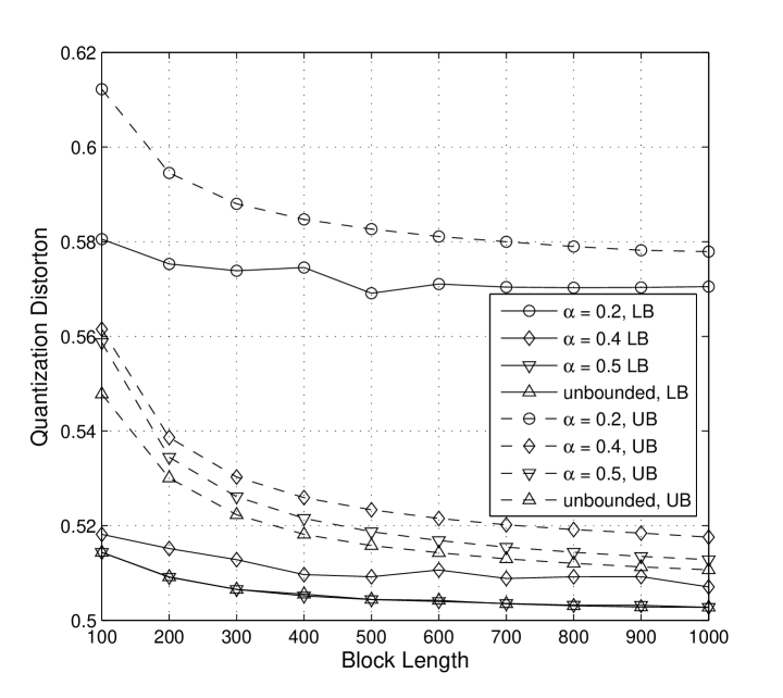
Figure 3: Distortion for the unit Gaussian Source with Quantization Rate $1/2$.

VIII Conclusions

We have proposed the upper and lower bounds of the optimal quantization for identically and independently distributed source in the finite-block length regime. The lower bound can be proved to be larger than the asymptotical distortion of the rate-distortion theory. The upper bounds can be proved to approach the asymptotical distortion of the rate-distortion theory. We have also applied the upper and lower bounds to binary symmetric source, binary non-symmetric source, and Gaussian source. Numerical results show reasonable gap between the upper and lower bounds.

One important open question is the one-curve approximation of the quantization distortion. For the finite-block length regime of the block error probability for channel codes, the one-curve Gaussian approximation is first proposed in [15] and then refined in [16], based on the Gaussian approximation of the Neyman-Pearson detection. For the rate-distortion counterparts, a possibly feasible way to solving this question is from the lower bound given by Corollary 3, which remains to be an open question for further research.

IX Appendix - Background Knowledge

IX-A Chi-squared and Non-centralized Chi-squared Distributions

IX-A1 Chi-squared Distribution

Consider $n$ independent Gaussian random variables $Z_{j}\sim{\cal N}(0,\sigma^{2}_{j})$ for $1\leq j\leq n$, and

$$Q=\sum^{n}_{j=1}\Big{(}\frac{Z_{j}}{\sigma_{j}}\Big{)}^{2}.$$ (242)

Then, $Q$ satisfies the order-$n$ Chi-squared distribution, denoted as $\chi^{2}(n)$.

The probability density function and cumulative distribution function for the order-$n$ Chi-squared distribution, denoted as $\upsilon_{n}(x)$ and $\Upsilon_{n}(x)$, respectively, are given as follows,

$$\upsilon_{n}(x) = \frac{1}{2^{n/2}\Gamma(n/2)}x^{n/2-1}e^{-x/2},\ \mbox{and}\ \Upsilon_{n}(x)=\int^{x}_{0}\upsilon_{n}(t)dt.$$ (243)

IX-A2 Non-centered Chi-squared Distribution

Consider $n$ independent Gaussian random variables $Z_{j}\sim{\cal N}(\mu_{j},\sigma^{2}_{j})$ for $1\leq j\leq n$. Let

$$Q=\sum^{n}_{j=1}\Big{(}\frac{Z_{j}}{\sigma_{j}}\Big{)}^{2},\ \mbox{and}\ \lambda=\sum^{n}_{j=1}\Big{(}\frac{\mu_{j}}{\sigma_{j}}\Big{)}^{2}.$$ (244)

Then, $Q$ satisfies the order-$n$ noncentral Chi-squared distribution with the noncentrality parameter $\lambda$. The probability density function and cumulative distribution function, denoted as $\upsilon_{n}(x,\lambda)$ and $\Upsilon_{n}(x,\lambda)$, respectively, are given as follows,

$$\upsilon_{n}(x,\lambda)=\sum^{+\infty}_{i=0}\frac{e^{-\lambda/2}(\lambda/2)^{i}}{i!}\upsilon_{n+2i}(x),\ \mbox{and}\ \Upsilon_{n}(x,\lambda)=\int^{x}_{0}\upsilon_{n}(t,\lambda)dt.$$ (245)

Another equivalent definition for non-centered Chi-squared distribution is given as follows. Consider $n$ independent Gaussian random variables $Z_{j}\sim{\cal N}(0,\sigma^{2}_{j})$ for $1\leq j\leq n$, and fixed $y_{j}$ for $1\leq j\leq n$. Let

$$Q=\sum^{n}_{j=1}\Big{(}\frac{Z_{j}-y_{j}}{\sigma_{j}}\Big{)}^{2}.$$ (246)

Then, $Q$ satisfies order-$n$ noncentral Chi-squared distribution with noncentrality parameter

$$\lambda=\sum^{n}_{j=1}\Big{(}\frac{y_{j}}{\sigma_{j}}\Big{)}^{2}.$$ (247)

IX-B Computational Methods for the Intersection of Two Balls

We introduce a methods for computing the volume and probability measure for the intersection of two balls. More specifically, we consider the following two balls

$${\cal C}_{0}=\{{\mbox{\boldmath$x$}}:\|{\mbox{\boldmath$x$}}\|^{2}\leq r^{2}_{0}\}\ \mbox{and}\ {\cal C}_{1}=\{{\mbox{\boldmath$x$}}:\|{\mbox{\boldmath$x$}}-{\mbox{\boldmath$x$}}_{1}\|^{2}\leq r^{2}_{1}\},$$ (248)

as well as the following Gaussian distribution,

$$p({\mbox{\boldmath$x$}})=\frac{1}{(2\pi\sigma^{2})^{\frac{n}{2}}}e^{-\frac{\|{\mbox{\boldmath$x$}}\|^{2}}{2\sigma^{2}}}.$$ (249)

For a set $S\subseteq\mathbb{R}^{n}$, let ${\cal V}_{n}(S)$ be the volume of $S$, and $\mathbb{P}(S)$ be the probability measure of $S$ under the distribution $p({\mbox{\boldmath$x$}})$. In the following we present a computational method for the volume and probability of ${\cal C}_{1}\setminus{\cal C}_{0}$ and ${\cal C}_{1}\cap{\cal C}_{0}$.

The area of a unit sphere in ${\cal R}^{n}$, denoted as $A_{n}$, is given as follows

$$A_{n}=\frac{2\pi^{n/2}}{\Gamma(n/2)};$$ (250)

and the volume of a unit ball, denoted as $V_{n}$, is given by

$$V_{n}=\frac{A_{n}}{n}=\frac{\pi^{n/2}}{\Gamma(1+n/2)}.$$ (251)

Figure 4: The illustration of a cone with semiangle $\theta$, the parts ${\cal C}_{1}\setminus{\cal C}_{0}$, and ${\cal C}_{1}\cap{\cal C}_{0}$.

IX-B1 Sphere Area of a Cone

Consider the radius-$r$ sphere in ${\cal R}^{n}$ cut out by a cone with semiangle $\theta$, as shown in Fig. 4 (a). The area of that cone, denoted as $\Omega_{n}(\theta)$, is given by

$$\Omega_{n}(\theta)=\frac{2\pi^{(n-1)/2}}{\Gamma((n-1)/2)}\int^{\theta}_{0}(\sin\phi)^{n-2}d\phi,$$ (252)

where $\Gamma(\cdot)$ is gamma function.

IX-B2 Volume and Probability of ${\cal C}_{1}\setminus{\cal C}_{0}$

The volume of ${\cal C}_{1}\setminus{\cal C}_{0}$ can be computed via integrating the intersection of a radius-$r$ sphere with ${\cal C}_{1}\setminus{\cal C}_{0}$. Note that the intersection is not empty for $r_{0}\leq r\leq\|{\mbox{\boldmath$x$}}_{1}\|+r_{1}$. The semiangle of the cone cut out, denoted as $\theta(r)$, can be specified by triangle with the lengths of three edges, $r$, $\|{\mbox{\boldmath$x$}}_{1}\|$, and $r_{1}$, where $\theta(r)$ is between the two edges of lengths $r$ and $\|{\mbox{\boldmath$x$}}_{1}\|$. Thus, we have

$$\theta(r)=\cos^{-1}\frac{\|{\mbox{\boldmath$x$}}_{1}\|^{2}+r^{2}-r^{2}_{1}}{2\|{\mbox{\boldmath$x$}}_{1}\|r};$$ (253)

and the area of the sphere cut out is given by $r^{n-1}\Omega_{n}(\theta(r))$.

The volume ${\cal V}_{n}\Big{(}{\cal C}_{1}\setminus{\cal C}_{0}\Big{)}$ is computed via integrating the area of radius-$r$ sphere with semi-angle $\theta(r)$ in the range $r_{0}\leq r\leq\|{\mbox{\boldmath$x$}}_{1}\|+r_{1}$, given by

$${\cal V}_{n}\Big{(}{\cal C}_{1}\setminus{\cal C}_{0}\Big{)}=\int^{\|{\mbox{\boldmath$x$}}_{1}\|+r_{1}}_{r_{0}}r^{n-1}\Omega_{n}(\theta(r))dr;$$ (254)

and the probability $\mathbb{P}_{n}\Big{(}{\cal C}_{1}\setminus{\cal C}_{0}\Big{)}$ is computed via integrating the area weighted by the probability density $p({\mbox{\boldmath$x$}})$ for $\|{\mbox{\boldmath$x$}}\|=r$, given by

$$\mathbb{P}\Big{(}{\cal C}_{1}\setminus{\cal C}_{0}\Big{)}=\int^{\|{\mbox{\boldmath$x$}}_{1}\|+r_{1}}_{r_{0}}\frac{1}{(2\pi\sigma^{2})^{\frac{n}{2}}}e^{-\frac{r^{2}}{2\sigma^{2}}}r^{n-1}\Omega_{n}(\theta(r))dr.$$ (255)

IX-B3 Volume and Probability of ${\cal C}_{1}\cap{\cal C}_{0}$ for $r_{1}\leq\|{\mbox{\boldmath$x$}}_{1}\|$

For $r_{1}\leq\|{\mbox{\boldmath$x$}}_{1}\|$, the center of ${\cal C}_{0}$ is not contained in the interior of ${\cal C}_{1}$, as shown in Fig. 4 (c). The volume is computed via integrating the area $r^{n-1}\Omega_{n}(\theta(r))$ among $\|{\mbox{\boldmath$x$}}_{1}\|-r_{1}\leq r\leq r_{0}$, where $\theta(r)$ is specified by (253), given by

$${\cal V}_{n}\Big{(}{\cal C}_{1}\cap{\cal C}_{0}\Big{)}=\int^{r_{0}}_{\|{\mbox{\boldmath$x$}}_{1}\|-r_{1}}r^{n-1}\Omega_{n}(\theta(r))dr;$$ (256)

and the probability $\mathbb{P}\Big{(}{\cal C}_{1}\setminus{\cal C}_{0}\Big{)}$ is computed via integrating the sphere area weighted by the probability density, given by

$$\mathbb{P}\Big{(}{\cal C}_{1}\cap{\cal C}_{0}\Big{)}=\int^{r_{0}}_{\|{\mbox{\boldmath$x$}}_{1}\|-r_{1}}\frac{1}{(2\pi\sigma^{2})^{\frac{n}{2}}}e^{-\frac{r^{2}}{2\sigma^{2}}}r^{n-1}\Omega_{n}(\theta(r))dr.$$ (257)

IX-B4 Volume and Probability of ${\cal C}_{1}\cap{\cal C}_{0}$ for $r_{1}\geq\|{\mbox{\boldmath$x$}}_{1}\|$

For $\|{\mbox{\boldmath$x$}}_{1}\|\geq r_{1}$, ${\cal C}_{1}\cap{\cal C}_{0}$ contains a ball of radius $\|{\mbox{\boldmath$x$}}_{1}\|-r_{1}$. The volume of the rest part can be computed via integrating $r^{n-1}\Omega_{n}(\theta(r))$ among $r_{1}-\|{\mbox{\boldmath$x$}}_{1}\|\leq r\leq r_{0}$, where $\theta(r)$ is specified by (253). Then, we have

$${\cal V}_{n}\Big{(}{\cal C}_{1}\cap{\cal C}_{0}\Big{)}=\Big{(}r_{1}-\|{\mbox{\boldmath$x$}}_{1}\|\Big{)}^{n}V_{n}+\int^{r_{0}}_{r_{1}-\|{\mbox{\boldmath$x$}}_{1}\|}r^{n-1}\Omega_{n}(\theta(r))dr;$$ (258)

and $\mathbb{P}\Big{(}{\cal C}_{1}\setminus{\cal C}_{0}\Big{)}$ can be computed by the sum probability of the two parts, given by

$$\mathbb{P}\Big{(}{\cal C}_{1}\cap{\cal C}_{0}\Big{)}=\Upsilon_{n}\Big{(}(\frac{r_{1}-\|{\mbox{\boldmath$x$}}_{1}\|}{\sigma})^{2}\Big{)}+\int^{r_{0}}_{r_{1}-\|{\mbox{\boldmath$x$}}_{1}\|}\frac{1}{(2\pi\sigma^{2})^{\frac{n}{2}}}e^{-\frac{r^{2}}{2\sigma^{2}}}r^{n-1}\Omega_{n}(\theta(r))dr.$$ (259)

X Appendix - Proof of Theorems

X-A Proof of Theorem 14

Let $s_{\mbox{\boldmath$x$}}=\min\{d({\mbox{\boldmath$x$}},{\mbox{\boldmath$y$}}_{b}),t_{\mbox{\boldmath$x$}}\}$. Then, from (79) and Theorem 13 we have that

$$\bar{F}({\mbox{\boldmath$x$}},s_{\mbox{\boldmath$x$}})\geq\epsilon^{\frac{1}{Q-2}},$$ (260)

and that the probability

$$\mathbb{P}\Big{(}d({\mbox{\boldmath$x$}},{\mbox{\boldmath$y$}})<s_{\mbox{\boldmath$x$}}\Big{)}\leq 1-\epsilon^{\frac{1}{Q-2}}.$$ (261)

Note that, due to the convexity of the function $\epsilon^{x}$ in terms of $x$, we have the following

$$\mathbb{P}\Big{(}d({\mbox{\boldmath$x$}},{\mbox{\boldmath$y$}})<s_{\mbox{\boldmath$x$}}\Big{)} \leq 1-\epsilon^{\frac{1}{Q-2}}=\epsilon^{0}-\epsilon^{\frac{1}{Q-2}}$$ (262)

$$\leq \frac{1}{Q-2}\frac{\partial\epsilon^{x}}{\partial x}\Big{|}_{x=0}=\frac{1}{Q-2}\ln\frac{1}{\epsilon}.$$

To prove (89), we have the following

$$\Delta\tilde{D}^{n}_{Q} \stackrel{{\scriptstyle\triangle}}{{=}} \int_{{\cal B}^{n}_{\epsilon}}p({\mbox{\boldmath$x$}})s_{\mbox{\boldmath$x$}}d{\mbox{\boldmath$x$}}-\int_{{\cal B}^{n}_{\epsilon}}\int p({\mbox{\boldmath$x$}})\hat{q}_{0}({\mbox{\boldmath$y$}}|{\mbox{\boldmath$x$}})d({\mbox{\boldmath$x$}},{\mbox{\boldmath$y$}})d{\mbox{\boldmath$y$}}d{\mbox{\boldmath$x$}}$$ (263)

$$\leq \int_{{\cal B}^{n}_{\epsilon}}p({\mbox{\boldmath$x$}})s_{\mbox{\boldmath$x$}}d{\mbox{\boldmath$x$}}-\int_{{\cal B}^{n}_{\epsilon}}\int p({\mbox{\boldmath$x$}})\hat{q}_{0}({\mbox{\boldmath$y$}}|{\mbox{\boldmath$x$}})d({\mbox{\boldmath$x$}},{\mbox{\boldmath$y$}})d{\mbox{\boldmath$y$}}d{\mbox{\boldmath$x$}}$$

$$= \int_{{\cal B}^{n}_{\epsilon}}p({\mbox{\boldmath$x$}})d{\mbox{\boldmath$x$}}\int\Big{(}s_{{\mbox{\boldmath$x$}}}-d({\mbox{\boldmath$x$}},{\mbox{\boldmath$y$}})\Big{)}\hat{q}_{0}({\mbox{\boldmath$y$}}|{\mbox{\boldmath$x$}})d{\mbox{\boldmath$y$}}$$

$$\leq \int_{{\cal B}^{n}_{\epsilon}}p({\mbox{\boldmath$x$}})d{\mbox{\boldmath$x$}}\int\Big{(}s_{{\mbox{\boldmath$x$}}}-d({\mbox{\boldmath$x$}},{\mbox{\boldmath$y$}})\Big{)}\hat{q}_{0}({\mbox{\boldmath$y$}}|{\mbox{\boldmath$x$}})\mathbf{1}_{s_{{\mbox{\boldmath$x$}}}>d({\mbox{\boldmath$x$}},{\mbox{\boldmath$y$}})}d{\mbox{\boldmath$y$}}.$$

Since for ${\mbox{\boldmath$x$}}\in{\cal B}^{n}_{\epsilon}$, $s_{\mbox{\boldmath$x$}}=\min\{d({\mbox{\boldmath$x$}},{\mbox{\boldmath$y$}}_{b}),t_{\mbox{\boldmath$x$}}\}\leq d({\mbox{\boldmath$x$}},{\mbox{\boldmath$y$}}_{b})\leq d+\epsilon$, we have

$$\Big{(}s_{{\mbox{\boldmath$x$}}}-d({\mbox{\boldmath$x$}},{\mbox{\boldmath$y$}})\Big{)}\cdot\mathbf{1}_{s_{{\mbox{\boldmath$x$}}}>d({\mbox{\boldmath$x$}},{\mbox{\boldmath$y$}})}\leq(\hat{d}+\epsilon)\cdot\mathbf{1}_{s_{{\mbox{\boldmath$x$}}}>d({\mbox{\boldmath$x$}},{\mbox{\boldmath$y$}})},$$ (264)

Based on this, we have the following to further bound $\Delta\tilde{D}_{Q}$ based on (263),

$$\Delta\tilde{D}^{n}_{Q} \leq \int_{{\cal B}^{n}_{\epsilon}}p({\mbox{\boldmath$x$}})\int(\hat{d}+\epsilon)\hat{q}_{0}({\mbox{\boldmath$y$}}|{\mbox{\boldmath$x$}})\mathbf{1}_{s_{{\mbox{\boldmath$x$}}}>d({\mbox{\boldmath$x$}},{\mbox{\boldmath$y$}})}d{\mbox{\boldmath$y$}}d{\mbox{\boldmath$x$}}$$ (265)

$$\leq (\hat{d}+\epsilon)\int\int p({\mbox{\boldmath$x$}})\hat{q}_{0}({\mbox{\boldmath$y$}}|{\mbox{\boldmath$x$}})\mathbf{1}_{s_{{\mbox{\boldmath$x$}}}>d({\mbox{\boldmath$x$}},{\mbox{\boldmath$y$}})}d{\mbox{\boldmath$y$}}d{\mbox{\boldmath$x$}}$$

$$= (\hat{d}+\epsilon)\int\int\hat{q}_{0}({\mbox{\boldmath$y$}})\hat{q}_{0}({\mbox{\boldmath$x$}}|{\mbox{\boldmath$y$}})\mathbf{1}_{s_{{\mbox{\boldmath$x$}}}>d({\mbox{\boldmath$x$}},{\mbox{\boldmath$y$}})}d{\mbox{\boldmath$y$}}d{\mbox{\boldmath$x$}}.$$

Using Holder inequality, we can further derive the upper bound for any $0<\beta<1$, as follows,

$$\Delta\tilde{D}^{n}_{Q} \leq (\hat{d}+\epsilon)\int\int\hat{q}_{0}({\mbox{\boldmath$y$}})\hat{q}_{0}({\mbox{\boldmath$x$}}|{\mbox{\boldmath$y$}})\mathbf{1}_{s_{{\mbox{\boldmath$x$}}}>d({\mbox{\boldmath$x$}},{\mbox{\boldmath$y$}})}d{\mbox{\boldmath$y$}}d{\mbox{\boldmath$x$}}$$ (266)

$$\leq (\hat{d}+\epsilon)\int\Big{(}\int\hat{q}({\mbox{\boldmath$y$}})\hat{q}_{0}({\mbox{\boldmath$x$}}|{\mbox{\boldmath$y$}})^{1/\beta}d{\mbox{\boldmath$y$}}\Big{)}^{\beta}\Big{(}\int\hat{q}({\mbox{\boldmath$y$}})\mathbf{1}_{s_{{\mbox{\boldmath$x$}}}>d({\mbox{\boldmath$x$}},{\mbox{\boldmath$y$}})}d{\mbox{\boldmath$y$}}\Big{)}^{1-\beta}d{\mbox{\boldmath$x$}}\ \mbox{[Holder]}$$

$$\leq (\hat{d}+\epsilon)\int\Big{(}\int\hat{q}_{0}({\mbox{\boldmath$y$}})\hat{q}_{0}({\mbox{\boldmath$x$}}|{\mbox{\boldmath$y$}})^{1/\beta}d{\mbox{\boldmath$y$}}\Big{)}^{\beta}\Big{(}\frac{1}{Q-2}\ln\frac{1}{\epsilon}\Big{)}^{1-\beta}d{\mbox{\boldmath$x$}}$$

$$\leq (\hat{d}+\epsilon)\ln\frac{1}{\epsilon}\int\Big{(}\int\hat{q}_{0}({\mbox{\boldmath$y$}})\hat{q}_{0}({\mbox{\boldmath$x$}}|{\mbox{\boldmath$y$}})^{1/\beta}d{\mbox{\boldmath$y$}}\Big{)}^{\beta}\Big{(}\frac{1}{Q-2}\Big{)}^{1-\beta}d{\mbox{\boldmath$x$}}$$

$$= (\hat{d}+\epsilon)\ln\frac{1}{\epsilon}\cdot\frac{2^{n(1-R)}}{2^{n(1-R)}-2}\Big{(}2^{-(1-\beta)R}\int\Big{(}\int\hat{q}_{0}(y)\hat{q}_{0}(x|y)^{1/\beta}dy\Big{)}^{\beta}dx\Big{)}^{n}.$$

Note that since [9],

$$\lim_{\beta\uparrow 1}\frac{\log_{2}\int\Big{(}\int\hat{q}_{0}(y)\hat{q}_{0}(x|y)^{1/\beta}dy\Big{)}^{\beta}dx}{1-\beta}=I(\hat{q}_{0})=R_{0},$$ (267)

we have that there exists a $\beta_{0}$ sufficient close to $1$, such that

$$\frac{\log_{2}\int\Big{(}\int\hat{q}_{0}(y)\hat{q}_{0}(x|y)^{1/\beta_{0}}dy\Big{)}^{\beta_{0}}dx}{1-\beta_{0}}<\frac{R+R_{0}}{2},$$ (268)

such that

$$2^{-(1-\beta_{0})R}\int\Big{(}\int\hat{q}_{0}(y)\hat{q}_{0}(x|y)^{1/\beta_{0}}dy\Big{)}^{\beta_{0}}dx<2^{-(1-\beta_{0})(R-R_{0})},$$ (269)

and thus

$$\Delta\tilde{D}^{n}_{Q}\leq(\hat{d}+\epsilon)\ln\frac{1}{\epsilon}\cdot 2^{-(1-\beta_{0})(R-R_{0})n}.$$ (270)

Finally, since $\tilde{D}_{0}<\infty$ [c.f. (88)], we have that

$$\tilde{D}^{n}_{Q}-\int\int p({\mbox{\boldmath$x$}})\hat{q}_{0}({\mbox{\boldmath$y$}}|{\mbox{\boldmath$x$}})d({\mbox{\boldmath$x$}},{\mbox{\boldmath$y$}})d{\mbox{\boldmath$x$}}d{\mbox{\boldmath$y$}}\leq(\hat{d}+\epsilon)\ln\frac{1}{\epsilon}\cdot 2^{-(1-\beta_{0})(R-R_{0})n}+\epsilon\tilde{D}_{0}.$$ (271)

Then, for sufficiently small $\zeta>0$, we select a sufficient small $\epsilon$, the second term $\epsilon\tilde{D}_{0}<\zeta/2$; and given the selected $\epsilon$, for sufficient large $n$ have that the first terms is also smaller than $\zeta/2$, and thus we have that

$$\tilde{D}^{n}_{Q}<\int\int p({\mbox{\boldmath$x$}})\hat{q}_{0}({\mbox{\boldmath$y$}}|{\mbox{\boldmath$x$}})d({\mbox{\boldmath$x$}},{\mbox{\boldmath$y$}})d{\mbox{\boldmath$x$}}d{\mbox{\boldmath$y$}}+\zeta.$$ (272)

X-B Proof of Theorem 20

For any ${\mbox{\boldmath$x$}}\in{\cal B}^{n}_{\delta}$, we let $\Psi({\mbox{\boldmath$x$}},{\mbox{\boldmath$y$}})=d+\delta$ for ${\mbox{\boldmath$y$}}\in A_{\mbox{\boldmath$x$}}(\gamma_{\mbox{\boldmath$x$}})$, $\Psi({\mbox{\boldmath$x$}},{\mbox{\boldmath$y$}})=l_{\mbox{\boldmath$x$}}$ for ${\mbox{\boldmath$y$}}\in\bar{A}_{\mbox{\boldmath$x$}}(\gamma_{\mbox{\boldmath$x$}})$, and $\Psi({\mbox{\boldmath$x$}},{\mbox{\boldmath$y$}})=0$ for ${\mbox{\boldmath$y$}}\in A^{c}_{\mbox{\boldmath$x$}}(\gamma_{\mbox{\boldmath$x$}})$; and thus we have that

$$\int\hat{q}_{0}({\mbox{\boldmath$y$}})\Psi({\mbox{\boldmath$x$}},{\mbox{\boldmath$y$}})d{\mbox{\boldmath$y$}}=\tilde{B}({\mbox{\boldmath$x$}}).$$ (273)

We can write the right side of (126) as follows

$$\int_{{\cal B}^{n}_{\delta}}p({\mbox{\boldmath$x$}})h^{U}({\mbox{\boldmath$x$}})d{\mbox{\boldmath$x$}} = \int_{{\cal B}^{n}_{\delta}}\int p({\mbox{\boldmath$x$}})\hat{q}_{0}({\mbox{\boldmath$y$}}|{\mbox{\boldmath$x$}})\Psi({\mbox{\boldmath$x$}},{\mbox{\boldmath$y$}})d{\mbox{\boldmath$x$}}d{\mbox{\boldmath$y$}}$$ (274)

$$= \int_{{\cal B}^{n}_{\delta}}\int\hat{q}_{0}({\mbox{\boldmath$y$}})\hat{q}_{0}({\mbox{\boldmath$x$}}|{\mbox{\boldmath$y$}})\Psi({\mbox{\boldmath$x$}},{\mbox{\boldmath$y$}})d{\mbox{\boldmath$x$}}d{\mbox{\boldmath$y$}}.$$

For any $0<\beta<1$, also from Holder inequality we have the following

$$\tilde{D}^{n}_{Q}-D(R_{0}) \leq \int_{{\cal B}^{n}_{\delta}}\int\hat{q}_{0}({\mbox{\boldmath$x$}})\hat{q}_{0}({\mbox{\boldmath$x$}}|{\mbox{\boldmath$y$}})\Psi({\mbox{\boldmath$x$}},{\mbox{\boldmath$y$}})d{\mbox{\boldmath$x$}}d{\mbox{\boldmath$y$}}$$ (275)

$$\leq \int_{{\cal B}^{n}_{\delta}}\Big{(}\int\hat{q}_{0}({\mbox{\boldmath$y$}})\hat{q}_{0}({\mbox{\boldmath$x$}}|{\mbox{\boldmath$y$}})^{1/\beta}d{\mbox{\boldmath$y$}}\Big{)}^{\beta}\Big{(}\int\hat{q}_{0}({\mbox{\boldmath$y$}})\Psi({\mbox{\boldmath$x$}},{\mbox{\boldmath$y$}})^{1/(1-\beta)}d{\mbox{\boldmath$y$}}\Big{)}^{1-\beta}d{\mbox{\boldmath$x$}}$$

$$\leq \int_{{\cal B}^{n}_{\delta}}\Big{(}\int\hat{q}_{0}({\mbox{\boldmath$y$}})\hat{q}_{0}({\mbox{\boldmath$x$}}|{\mbox{\boldmath$y$}})^{1/\beta}d{\mbox{\boldmath$y$}}\Big{)}^{\beta}\Big{(}\int\hat{q}_{0}({\mbox{\boldmath$y$}})\Psi({\mbox{\boldmath$x$}},{\mbox{\boldmath$y$}})(d+\delta)^{\beta/(1-\beta)}d{\mbox{\boldmath$y$}}\Big{)}^{1-\beta}d{\mbox{\boldmath$x$}}$$

$$= (d+\delta)^{\beta}\int_{{\cal B}^{n}_{\delta}}\Big{(}\int\hat{q}_{0}({\mbox{\boldmath$y$}})\hat{q}_{0}({\mbox{\boldmath$x$}}|{\mbox{\boldmath$y$}})^{1/\beta}d{\mbox{\boldmath$y$}}\Big{)}^{\beta}\Big{(}\int\hat{q}_{0}({\mbox{\boldmath$y$}})\Psi({\mbox{\boldmath$x$}},{\mbox{\boldmath$y$}})d{\mbox{\boldmath$y$}}\Big{)}^{1-\beta}d{\mbox{\boldmath$x$}}$$

$$\leq (d+\delta)^{\beta}\int_{{\cal B}^{n}_{\delta}}\Big{(}\int\hat{q}_{0}({\mbox{\boldmath$y$}})\hat{q}_{0}({\mbox{\boldmath$x$}}|{\mbox{\boldmath$y$}})^{1/\beta}d{\mbox{\boldmath$y$}}\Big{)}^{\beta}\Big{(}\frac{\mathbb{E}\Big{(}\rho^{0}_{\mbox{\boldmath$x$}}\Big{)}}{Q(e-\eta)}\Big{)}^{1-\beta}d{\mbox{\boldmath$x$}}$$

$$\leq (d+\delta)^{\beta}\Big{(}\frac{d+\delta}{e-\eta}\Big{)}^{1-\beta}\frac{1}{Q^{1-\beta}}\int_{{\cal B}^{n}_{\delta}}\Big{(}\int\hat{q}_{0}({\mbox{\boldmath$y$}})\hat{q}_{0}({\mbox{\boldmath$x$}}|{\mbox{\boldmath$y$}})^{1/\beta}d{\mbox{\boldmath$y$}}\Big{)}^{\beta}d{\mbox{\boldmath$x$}}$$

$$\leq \frac{d+\delta}{(e-\eta)^{1-\beta}}\frac{1}{Q^{1-\beta}}\int\Big{(}\int\hat{q}_{0}({\mbox{\boldmath$y$}})\hat{q}_{0}({\mbox{\boldmath$x$}}|{\mbox{\boldmath$y$}})^{1/\beta}d{\mbox{\boldmath$y$}}\Big{)}^{\beta}d{\mbox{\boldmath$x$}}$$

$$\leq l_{m}^{\beta}\Big{(}\frac{\rho_{m}}{e-\eta}\Big{)}^{1-\beta}\Big{(}2^{-(1-\beta)R}\int\Big{(}\int\hat{q}_{0}(y)\hat{q}_{0}(x|y)^{1/\beta}dy\Big{)}^{\beta}dx\Big{)}^{n}.$$

Then, similar to the arguments in the proof of Theorem 14, we have that for $\beta$ sufficient close to $1$,

$$2^{-(1-\beta)R}\int\Big{(}\int\hat{q}_{0}(y)\hat{q}_{0}(x|y)^{1/\beta}dy\Big{)}^{\beta}dx<1,$$ (276)

and thus according to (275), the upper bound of $\tilde{D}_{Q}-D(\hat{q})$ exponentially attenuates with the codeword block length $n$.

X-C Proof of Theorem 32

Note that

$${\cal V}_{n}\Big{(}\cup^{Q}_{j=0}{\cal C}_{j}(t)\Big{)}\leq{\cal V}_{n}\Big{(}{\cal C}_{0}(t)\Big{)}+\sum^{Q}_{j=1}{\cal V}_{n}\Big{(}{\cal C}_{j}(t)\setminus{\cal C}_{0}(t)\Big{)}.$$ (277)

Then we need to prove that

$${\cal V}_{n}\Big{(}{\cal C}_{j}(t)\setminus{\cal C}_{0}(t)\Big{)}\leq{\cal V}_{n}\Big{(}\tilde{\cal C}_{j}(t)\setminus{\cal C}_{0}(t)\Big{)}.$$ (278)

Note that, for ${\cal C}_{j}(t)$ the center and radius are ${\mbox{\boldmath$y$}}_{j}$ and $\sqrt{R(t,\|{\mbox{\boldmath$y$}}_{j}\|)}$, respectively; and for $\tilde{\cal C}_{j}(t)$ they are $\tilde{\mbox{\boldmath$y$}}_{j}$ and $\sqrt{R(t,R_{m})}$, respectively. We define another ball with center ${\mbox{\boldmath$y$}}_{j}$ and radius $\sqrt{R(t,R_{m})}$, denoted as $\hat{\cal C}_{j}(t)$. Then, we can prove

$${\cal V}_{n}\Big{(}{\cal C}_{j}(t)\setminus{\cal C}_{0}(t)\Big{)}\leq{\cal V}_{n}\Big{(}\hat{\cal C}_{j}(t)\setminus{\cal C}_{0}(t)\Big{)}\leq{\cal V}_{n}\Big{(}\tilde{\cal C}_{j}(t)\setminus{\cal C}_{0}(t)\Big{)}.$$ (279)

The first inequality follows that fixing the center the volume ${\cal V}_{n}\Big{(}\hat{\cal C}_{j}(t)\setminus{\cal C}_{0}(t)\Big{)}$ increases via increasing radius from $\sqrt{R(t,\|{\mbox{\boldmath$y$}}_{j}\|)}$ to $\sqrt{R(t,R_{m})}$; and the second inequality follows that fixing the radius the volume ${\cal V}_{n}\Big{(}\tilde{\cal C}_{j}(t)\setminus{\cal C}_{0}(t)\Big{)}$ increases via increasing the distance between the centers of the two balls. Then, from (277) and (279) we have

$${\cal V}_{n}\Big{(}\cup^{Q}_{j=0}{\cal C}_{j}(t)\Big{)}\leq{\cal V}_{n}\Big{(}{\cal C}_{0}(t)\Big{)}+\sum^{Q}_{j=1}{\cal V}_{n}\Big{(}\tilde{\cal C}_{j}(t)\setminus{\cal C}_{0}(t)\Big{)}.$$ (280)

Via letting $\bar{V}_{n}={\cal V}_{n}\Big{(}\cup^{Q}_{j=0}{\cal C}_{j}(t)\Big{)}$, then according to $\bar{V}_{n}\leq\tilde{V}_{n}$ [c.f. (199)], we have

$$\mathbb{P}\Big{(}\cup^{Q}_{j=0}{\cal C}_{j}(t)\Big{)}\leq\max_{S,{\cal V}_{n}(S)\leq\bar{V}_{n}}\mathbb{P}\Big{(}S\Big{)}\leq\max_{S,{\cal V}_{n}(S)\leq\tilde{V}_{n}}\mathbb{P}\Big{(}S\Big{)}.$$ (281)

It is well known that, the given the volume ${\cal V}_{n}(S)$, the set $S$ that maximizes $\mathbb{P}\Big{(}S\Big{)}$ is the ball centered at the origin. Note that the radius of such ball is given by

$$r_{n}=\Big{(}\frac{\tilde{V}_{n}}{V_{n}}\Big{)}^{\frac{1}{n}};$$ (282)

and the probability mass is given by the chi-square cdf $\Upsilon_{n}(r^{2}_{n})$. Thus we have

$$\mathbb{P}\Big{(}\cup^{Q}_{j=0}{\cal C}_{j}(t)\Big{)}\leq\max_{S,{\cal V}_{n}(S)\leq\tilde{V}_{n}}\mathbb{P}\Big{(}S\Big{)}=\Upsilon_{n}(r^{2}_{n}).$$ (283)

Also, since for all ${\mbox{\boldmath$x$}}\in\cup^{Q}_{j=0}{\cal C}_{j}(t)$, there exist a $j$, $0\leq j\leq Q$, such that $\|{\mbox{\boldmath$x$}}-\frac{\sigma^{2}}{\sigma^{2}-D}{\mbox{\boldmath$y$}}_{j}\|\leq\sqrt{R(t,\|{\mbox{\boldmath$y$}}_{j}\|)}$, and thus

$$\|{\mbox{\boldmath$x$}}\|\leq\frac{\sigma^{2}}{\sigma^{2}-D}\|{\mbox{\boldmath$y$}}_{j}\|+\sqrt{R(t,\|{\mbox{\boldmath$y$}}_{j}\|)}\stackrel{{\scriptstyle\triangle}}{{=}}\tilde{r}_{n},$$ (284)

and thus the probability

$$\mathbb{P}\Big{(}\cup^{Q}_{j=0}{\cal C}_{j}(t)\Big{)}\leq\mathbb{P}\Big{(}\|{\mbox{\boldmath$x$}}\|\leq\tilde{r}_{n}\Big{)}=\Upsilon_{n}(\tilde{r}^{2}_{n}).$$ (285)

Therefore, from (283) and (285), we have that

$$\mathbb{P}\Big{(}\cup^{Q}_{j=0}{\cal C}_{j}(t)\Big{)}\leq\min\Big{\{}\Upsilon_{n}(r^{2}_{n}),\Upsilon_{n}(\tilde{r}^{2}_{n})\Big{\}}=\Upsilon_{n}(\tilde{r}^{2}_{E}),$$ (286)

where $r_{E}=\min\{r_{n},\tilde{r}_{n}\}$.

References

• [1] T. M. Cover and J. A. Thomas, Elements of Information Theory, 2nd ed.   Wiley Interscience, 2006.
• [2] R. Ahlswede, “Extremal properties of rate-distortion functions,” IEEE Trans. Info. Theory, vol. 36, no. 1, pp. 166–171, Jan. 1990.
• [3] M. T. Harrison and I. Kontoyiannis, “Estimation of the rate distortion function,” IEEE Trans. Info. Theory, vol. 54, no. 8, pp. 3757–3762, Aug. 2008.
• [4] D. Krithivasan and S. S. Pradhan, “Distributed source coding using abelian group codes: A new achievable rate-distortion region,” IEEE Trans. Info. Theory, vol. 57, no. 3, pp. 1495–1519, Mar. 2011.
• [5] R. Venkataramanan and S. S. Pradhan, “Source coding with feed-forward: Rate-distortion theorems and error exponents for a general source,” IEEE Trans. Info. Theory, vol. 53, no. 6, pp. 2154–2179, Jun. 2007.
• [6] Y.-Q. Zhang, R. L. Pickholtz, and M. H. Leow, “Rate-distortion bound for a class of non-gaussian sources with memory,” IEEE Trans. Info. Theory, vol. 39, no. 5, pp. 1697–1701, Sept. 2003.
• [7] A. Buzo, F. Kuhlmann, and C. Rivera, “Rate-distortion bounds for quotient-based distortions with application to itakura-saito distortion measures,” IEEE Trans. Info. Theory, vol. IT-32, no. 2, pp. 141–147, Mar. 1986.
• [8] N. Merhav, “On list size exponents in rate-distortion coding,” IEEE Trans. Info. Theory, vol. 43, no. 2, pp. 765–769, Feb. 1997.
• [9] J. K. Omura, “A coding theorem for discrete-time sources,” IEEE Trans. Info. Theory, vol. IT-19, no. 4, pp. 490–498, Jul. 1973.
• [10] I. Hen and N. Merhav, “On the error exponent of trellis source coding,” IEEE Trans. Info. Theory, vol. 51, no. 11, pp. 3734–3741, Nov. 2005.
• [11] T. Weissman and N. Merhav, “Tradeoffs between the excess-code-length exponent and the excess-distortion exponent in lossy source coding,” IEEE Trans. Info. Theory, vol. 48, no. 2, pp. 396–415, Feb. 2002.
• [12] T. Weissman, “Universally attainable error exponents for rate-distortion coding of noisy sources,” IEEE Trans. Info. Theory, vol. 50, no. 6, pp. 1229–1246, Jun. 2004.
• [13] S. Boyd and L. Vandenberghe, Convex Optimization.   Cambridge University Press, 2004.
• [14] T. BerGer, “Rate distortion theory for sources with abstract alphabets and memory,” Informaiton and Control, vol. 13, pp. 254–273, 1968.
• [15] V. Strassen, “Asymptotische abschatzungen in shannons informationstheorie,” in Trans. Third Prague Conf. Information Theory, Prague, 1962, pp. 689–723.
• [16] Y. Polyanskiy, H. V. Poor, and S. Verdu, “Channel coding rate in the finite blocklength regime,” IEEE Trans. Info. Theory, vol. 56, no. 5, pp. 2307–2359, May 2010.