Pinning consensus in networks of multiagents via a single impulsive controller

Bo Liu, Wenlian Lu and  Tianping Chen This work is jointly supported by the National Natural Sciences Foundation of China under Grant Nos. 61273211, 60974015, and 61273309, the Foundation for the Author of National Excellent Doctoral Dissertation of P.R. China No. 200921, the Shanghai Rising-Star Program (No. 11QA1400400), the Marie Curie International Incoming Fellowship from the European Commission (FP7-PEOPLE-2011-IIF-302421), and China Postdoctoral Science Foundation No. 2011M500065.Bo Liu is with School of Mathematical Sciences, Fudan University, Shanghai, People’s Republic of China, and Institute of Industrial Science, The University of Tokyo, 4-6-1 Komaba, Meguro-ku, Tokyo 153-8505, Japan (liu7bo9@gmail.com).Wenlian Lu is with Centre for Computational Systems Biology, and Laboratory of Mathematics for Nonlinear Science, School of Mathematical Sciences, Fudan University, Shanghai, People’s Republic of China (wenlian@fudan.edu.cn).Tianping Chen is with the School of Mathematical Sciences, Fudan University, 200433, Shanghai, China. (Corresponding author, email: tchen@fuan.edu.cn).
Abstract

In this paper, we discuss pinning consensus in networks of multiagents via impulsive controllers. In particular, we consider the case of using only one impulsive controller. We provide a sufficient condition to pin the network to a prescribed value. It is rigorously proven that in case the underlying graph of the network has spanning trees, the network can reach consensus on the prescribed value when the impulsive controller is imposed on the root with appropriate impulsive strength and impulse intervals. Interestingly, we find that the permissible range of the impulsive strength completely depends on the left eigenvector of the graph Laplacian corresponding to the zero eigenvalue and the pinning node we choose. The impulses can be very sparse, with the impulsive intervals being lower bounded. Examples with numerical simulations are also provided to illustrate the theoretical results.

Index Terms:
consensus, synchronization, multiagent systems, impulsive pinning control.

I Introduction

Coordinated and cooperative control of teams of autonomous systems has received much attention in recent years. Significant research activity has been devoted to this area. In the cooperation, group of agents seek to reach agreement on a certain quantity of interest. This is the so-called consensus problem, which has a long history in computer science. Recently, consensus problem reappeared in the cooperative control of multi-agent systems and has gained renewed interests due to the broad applications of multi-agent systems. A great deal of papers have addressed this problem. For a review of this area, see the surveys [1, 2] and references therein.

The basic idea of consensus is that each agent updates its state based on the states of its neighbors and its own such that the states of all agents will converge to a common value. The interaction rule that specifies the information exchange between an agent and its neighbors is called the consensus algorithm.

The following is an example of continuous-time consensus algorithm:

x˙i(t)=j=1,jinaij[xj(t)xi(t)],i=1,,nformulae-sequencesubscript˙𝑥𝑖𝑡superscriptsubscriptformulae-sequence𝑗1𝑗𝑖𝑛subscript𝑎𝑖𝑗delimited-[]subscript𝑥𝑗𝑡subscript𝑥𝑖𝑡𝑖1𝑛\displaystyle\dot{x}_{i}(t)=\sum_{j=1,j\neq i}^{n}a_{ij}[x_{j}(t)-x_{i}(t)],i=1,\cdots,n (1)

where xi(t)subscript𝑥𝑖𝑡x_{i}(t)\in{\mathbb{R}} is the state of agent i𝑖i at time t𝑡t, aij0subscript𝑎𝑖𝑗0a_{ij}\geq 0 for ij𝑖𝑗i\neq j is the coupling strength from agent j𝑗j to agent i𝑖i.

Let aii=j=1,jinaijsubscript𝑎𝑖𝑖superscriptsubscriptformulae-sequence𝑗1𝑗𝑖𝑛subscript𝑎𝑖𝑗a_{ii}=-\sum_{j=1,j\neq i}^{n}a_{ij} for i=1,2,,n𝑖12𝑛i=1,2,\cdots,n, we can have

x˙i(t)=j=1naijxj(t),i=1,,n.formulae-sequencesubscript˙𝑥𝑖𝑡superscriptsubscript𝑗1𝑛subscript𝑎𝑖𝑗subscript𝑥𝑗𝑡𝑖1𝑛\displaystyle\dot{x}_{i}(t)=\sum_{j=1}^{n}a_{ij}x_{j}(t),~{}i=1,\cdots,n. (2)

A topic closely related to consensus is synchronization, which can be written as the following Linearly Coupled Ordinary Differential Equations (LCODEs):

dxi(t)dt=f(xi(t),t)+cj=1naijxj(t),i=1,,nformulae-sequence𝑑superscript𝑥𝑖𝑡𝑑𝑡𝑓superscript𝑥𝑖𝑡𝑡𝑐superscriptsubscript𝑗1𝑛subscript𝑎𝑖𝑗superscript𝑥𝑗𝑡𝑖1𝑛\displaystyle\frac{dx^{i}(t)}{dt}=f(x^{i}(t),t)+c\sum\limits_{j=1}^{n}a_{ij}x^{j}(t),\quad i=1,\cdots,n (3)

where xi(t)msuperscript𝑥𝑖𝑡superscript𝑚x^{i}(t)\in{\mathbb{R}}^{m} is the state variable of the i𝑖ith node at time t𝑡t, f𝑓f: m×[0,+)msuperscript𝑚0superscript𝑚{\mathbb{R}}^{m}\times[0,+\infty)\rightarrow\mathbb{R}^{m} is a continuous map, A=[aij]n×n𝐴delimited-[]subscript𝑎𝑖𝑗superscript𝑛𝑛A=[a_{ij}]\in{\mathbb{R}}^{n\times n} is the coupling matrix with zero-sum rows and aij0subscript𝑎𝑖𝑗0a_{ij}\geq 0, for ij𝑖𝑗i\neq j, which is determined by the topological structure of the LCODEs.

There are lots of papers discussing synchronization in various circumstances.

It is clear that the consensus is a special case of synchronization (f=0𝑓0f=0, m=1𝑚1m=1). Therefore, all the results concerning synchronization can apply to consensus.

It was shown in [3, 4] that under some assumptions, we have

limtxi(t)j=1nξjxj(t)=0,i=1,,n,formulae-sequencesubscript𝑡normsuperscript𝑥𝑖𝑡superscriptsubscript𝑗1𝑛subscript𝜉𝑗superscript𝑥𝑗𝑡0𝑖1𝑛\displaystyle\lim_{t\rightarrow\infty}||x^{i}(t)-\sum_{j=1}^{n}\xi_{j}x^{j}(t)||=0,~{}~{}i=1,\cdots,n, (4)

where [ξ1,,ξn]superscriptsubscript𝜉1subscript𝜉𝑛top[\xi_{1},\cdots,\xi_{n}]^{\top} is the left eigenvector of A𝐴A corresponding to the eigenvalue 00 satisfying j=1nξj=1superscriptsubscript𝑗1𝑛subscript𝜉𝑗1\sum_{j=1}^{n}\xi_{j}=1.

Since in the consensus model,

j=1nξjxj(t)=j=1nξjxj(0)superscriptsubscript𝑗1𝑛subscript𝜉𝑗subscript𝑥𝑗𝑡superscriptsubscript𝑗1𝑛subscript𝜉𝑗subscript𝑥𝑗0\displaystyle\sum_{j=1}^{n}\xi_{j}x_{j}(t)=\sum_{j=1}^{n}\xi_{j}x_{j}(0) (5)

for all t>0𝑡0t>0, we have

limt|xi(t)j=1nξjxj(0)|=0,i=1,,n.formulae-sequencesubscript𝑡subscript𝑥𝑖𝑡superscriptsubscript𝑗1𝑛subscript𝜉𝑗subscript𝑥𝑗00𝑖1𝑛\displaystyle\lim_{t\rightarrow\infty}|x_{i}(t)-\sum_{j=1}^{n}\xi_{j}x_{j}(0)|=0,~{}~{}i=1,\cdots,n. (6)

It can be seen that the agreement value j=1nξjxj(0)superscriptsubscript𝑗1𝑛subscript𝜉𝑗subscript𝑥𝑗0\sum_{j=1}^{n}\xi_{j}x_{j}(0) strongly depends on the initial value, which means that the agreement value of the consensus algorithm is neutral stable (or semi-stable used in some papers). The concept of neutral stability is used in physics and other research fields. For example, the principal subspace extraction algorithms and principal component extraction algorithms discussed in [5, 6]. A set of equilibrium points is called neutral stable for a system, if each equilibrium is Lyapunov stable, and every trajectory that starts in a neighborhood of an equilibrium converges to a possibly different equilibrium. Similarly, a set of manifolds is called neutral stable for a system, if every manifold is invariant, and when there is a small perturbation, the state will stay in another manifold and never return.

In [5], the manifold discussed is neutral stable, and if the algorithm is restricted to the manifold, the equilibrium is stable. Instead, in [6], the equilibrium is neutral stable and the Stiefel manifold is stable.

In consensus algorithm, the consensus manifold S={xn:x1=x2==xn}𝑆conditional-set𝑥superscript𝑛subscript𝑥1subscript𝑥2subscript𝑥𝑛S=\{x\in\mathbb{R}^{n}:~{}x_{1}=x_{2}=\cdots=x_{n}\} is the set of equilibrium points, which is stable. Instead, every point xS𝑥𝑆x\in S is neutral stable.

However, in some cases, it is desired that all states converge to a prescribed value, say, some s𝑠s\in\mathbb{R}. For example, in a military system, if one wants to use a missile network to attack some object of the enemy, then it is required that all the missiles from different military bases should finally hit the same point (see [19]). Generally, for this purpose, one can make every state xi(t)subscript𝑥𝑖𝑡x_{i}(t) converge to s𝑠s by imposing a negative feedback term [xi(t)s]delimited-[]subscript𝑥𝑖𝑡𝑠-[x_{i}(t)-s] to agent i𝑖i. However, due to the interaction of the network, it is not necessary to impose controllers on all the nodes. This is the basic idea of the pining control technique, which is an effective class of control schemes. Generally, in a pinning control scheme, we only need to impose controllers on a small fraction of the nodes. This is a big advantage because in large complex networks, it is usually difficult if not impossible to add controllers to all the nodes. Recently, pinning strategies have been used in the control of dynamical networks. For example, decentralized adaptive pinning strategies have been proposed in [26, 27] for controlled synchronization of complex networks. And pinning consensus algorithms have been proposed in [10, 20].

Most works on pinning control consider pining a fraction of the nodes. However, there are a few works that consider pinning only one node. In [7], it was proved that if ε>0𝜀0\varepsilon>0, the following coupled network with a single controller

{dx1(t)dt=f(x1(t),t)+cj=1na1jxj(t)cε[x1(t)s(t)],dxi(t)dt=f(xi(t),t)+cj=1naijxj(t),i=2,,ncases𝑑superscript𝑥1𝑡𝑑𝑡absent𝑓superscript𝑥1𝑡𝑡𝑐superscriptsubscript𝑗1𝑛subscript𝑎1𝑗superscript𝑥𝑗𝑡missing-subexpression𝑐𝜀delimited-[]superscript𝑥1𝑡𝑠𝑡𝑑superscript𝑥𝑖𝑡𝑑𝑡absent𝑓superscript𝑥𝑖𝑡𝑡𝑐superscriptsubscript𝑗1𝑛subscript𝑎𝑖𝑗superscript𝑥𝑗𝑡missing-subexpression𝑖2𝑛\displaystyle\left\{\begin{array}[]{cc}\displaystyle\frac{dx^{1}(t)}{dt}&=f(x^{1}(t),t)+c\sum\limits_{j=1}^{n}a_{1j}x^{j}(t)\\ &-c\varepsilon[x^{1}(t)-s(t)],\\ \displaystyle\frac{dx^{i}(t)}{dt}&=f(x^{i}(t),t)+c\sum\limits_{j=1}^{n}a_{ij}x^{j}(t),\\ &i=2,\cdots,n\end{array}\right. (11)

can pin the complex dynamical network (3)3(\ref{synn}) to s(t)𝑠𝑡s(t), if c𝑐c is chosen suitably. Therefore, the following coupled network with a single controller

{x˙1(t)=j=1naijxj(t)ϵ[x1(t)s],x˙i(t)=j=1naijxj(t),i=2,,ncasesmissing-subexpressionsubscript˙𝑥1𝑡superscriptsubscript𝑗1𝑛subscript𝑎𝑖𝑗subscript𝑥𝑗𝑡italic-ϵdelimited-[]subscript𝑥1𝑡𝑠missing-subexpressionformulae-sequencesubscript˙𝑥𝑖𝑡superscriptsubscript𝑗1𝑛subscript𝑎𝑖𝑗subscript𝑥𝑗𝑡𝑖2𝑛\displaystyle\left\{\begin{array}[]{ll}&\dot{x}_{1}(t)=\sum_{j=1}^{n}a_{ij}x_{j}(t)-\epsilon[x_{1}(t)-s],\\ &\dot{x}_{i}(t)=\sum_{j=1}^{n}a_{ij}x_{j}(t),~{}~{}i=2,\cdots,n\end{array}\right. (14)

can make every state xi(t)subscript𝑥𝑖𝑡x_{i}(t) converge to s𝑠s.

It is worth noticing that the above mentioned works all consider continuous time feedback controllers and the disadvantage of such controllers lies in that the controller must be imposed at every time t𝑡t. So it is not applicable to systems which can not endure continuous disturbances. One can ask if we can pin the network only at a very sparse time sequence to make every state xi(t)subscript𝑥𝑖𝑡x_{i}(t) converge to s𝑠s for the consensus algorithm (2).

Actually, to avoid such disadvantages, some discontinuous control schemes, such as act-and-wait concept control[11, 12], intermittent control[13, 14] and impulsive technique[9, 15, 16, 17, 18] have already been developed and used in the control of dynamical systems. Particularly, in recent years, impulsive technique has been successfully used in many areas such as neural networks[9], control of spacecraft[16], secure communications[17] and so on.

Compared to continuous-time controllers, impulsive controllers have some obvious advantages. First, we only need to impose controllers at a very sparse sequence of time points. Besides, it is typically simpler and easier to implement. Recently, impulsive control techniques have been used in the controlled synchronization and consensus of complex networks. For example, in [24], an impulsive distributed control scheme was proposed to synchronize dynamical complex networks with both system delay and multiple coupling delays. In [23], impulsive control technique has been used in projective synchronization of drive-response networks of coupled chaotic systems. In [25], the authors used impulsive control technique to synchronize stochastic discrete-time networks. In [19], the authors proposed an impulsive hybrid control scheme for the consensus of a network with nonidentical nodes. Yet in these works, the controllers are imposed on all the nodes of the networks. To take advantage of both the impulsive and pinning control techniques, impulsive pinning technique has been proposed which combines these two control techniques as a whole. That is, the impulsive controllers are imposed only on a small fraction of the nodes. For example, in [21, 22], impulsive pinning control technique is used to stabilize and synchronize complex networks of dynamical systems. In this paper, we will introduce this technique into the pinning consensus algorithm. We show if the underlying graph has spanning trees, then a single impulsive controller imposed on one root is able to drive the network to reach consensus on a given value when the impulsive strength is in a permissible range and the impulse is sparse enough.

The rest of the paper is organized as follows. In Section II, some mathematical preliminaries are presented; In Section III, the sufficient conditions for pinning consensus via one impulsive controller on strongly connected graphs are proposed and proved; The results are extended to graphs with spanning trees in Section IV; Examples with numerical simulations are provided in Section V to illustrate the theoretical results; And the paper is concluded in Section VI.

II Mathematical preliminaries

In this section, we present some notations, definitions and lemmas concerning matrix and graph theory that will be used later.

First, we introduce following definitions and notations from [4].

Definition 1

Suppose A=[aij]i,j=1nn×n𝐴superscriptsubscriptdelimited-[]subscript𝑎𝑖𝑗𝑖𝑗1𝑛superscript𝑛𝑛A=[a_{ij}]_{i,j=1}^{n}\in\mathbb{R}^{n\times n}. If

  1. 1.

    aij0,ij,aii=j=1,jinaij,i=1,,nformulae-sequencesubscript𝑎𝑖𝑗0formulae-sequence𝑖𝑗formulae-sequencesubscript𝑎𝑖𝑖superscriptsubscriptformulae-sequence𝑗1𝑗𝑖𝑛subscript𝑎𝑖𝑗𝑖1𝑛a_{ij}\geq 0,\quad i\neq j,\qquad a_{ii}=-\sum\limits_{j=1,j\neq i}^{n}a_{ij},\quad i=1,\cdots,n;

  2. 2.

    real parts of eigenvalues of A𝐴A are all negative except an eigenvalue 00 with multiplicity 111,

then we say A𝐀1𝐴subscript𝐀1A\in{\bf A}_{1}.

Definition 2

Suppose A=[aij]i,j=1nn×n𝐴superscriptsubscriptdelimited-[]subscript𝑎𝑖𝑗𝑖𝑗1𝑛superscript𝑛𝑛A=[a_{ij}]_{i,j=1}^{n}\in\mathbb{R}^{n\times n}. If

  1. 1.

    aij0,ij,aii=j=1,jinaij,i=1,,nformulae-sequencesubscript𝑎𝑖𝑗0formulae-sequence𝑖𝑗formulae-sequencesubscript𝑎𝑖𝑖superscriptsubscriptformulae-sequence𝑗1𝑗𝑖𝑛subscript𝑎𝑖𝑗𝑖1𝑛a_{ij}\geq 0,\quad i\neq j,\qquad a_{ii}=-\sum\limits_{j=1,j\neq i}^{n}a_{ij},\quad i=1,\cdots,n;

  2. 2.

    A𝐴A is irreducible.

Then we say A𝐀2𝐴subscript𝐀2A\in{\mathbf{A}}_{2}.

It is clear that 𝐀2𝐀1subscript𝐀2subscript𝐀1\mathbf{A}_{2}\subseteq\mathbf{A}_{1}.

By Gersgorin theorem and Perron Frobenius theorem, we have the following result.

Lemma 1

[4]. If A𝐀1𝐴subscript𝐀1A\in\mathbf{A}_{1}, then the following items are valid:

  1. 1.

    If λ𝜆\lambda is an eigenvalue of A𝐴A and λ0𝜆0\lambda\neq 0, then Re(λ)<0𝑅𝑒𝜆0Re(\lambda)<0;

  2. 2.

    A𝐴A has an eigenvalue 00 with multiplicity 1 and the right eigenvector [1,1,,1]superscript111top[1,1,\dots,1]^{\top};

  3. 3.

    Suppose ξ=[ξ1,ξ2,,ξn]n𝜉superscriptsubscript𝜉1subscript𝜉2subscript𝜉𝑛topsuperscript𝑛\xi=[\xi_{1},\xi_{2},\cdots,\xi_{n}]^{\top}\in\mathbb{R}^{n} (without loss of generality, assume i=1nξi=1superscriptsubscript𝑖1𝑛subscript𝜉𝑖1\sum\limits_{i=1}^{n}\xi_{i}=1) is the left eigenvector of A𝐴A corresponding to eigenvalue 00. Then, ξi0subscript𝜉𝑖0\xi_{i}\geq 0 holds for all i=1,,n𝑖1𝑛i=1,\cdots,n; more precisely,

  4. 4.

    A𝐀2𝐴subscript𝐀2A\in\mathbf{A}_{2} if and only if ξi>0subscript𝜉𝑖0\xi_{i}>0 holds for all i=1,,n𝑖1𝑛i=1,\cdots,n;

  5. 5.

    A𝐴A is reducible if and only if for some i𝑖i, ξi=0subscript𝜉𝑖0\xi_{i}=0. In such case, by suitable rearrangement, assume that ξ=[ξ+,ξ0]superscript𝜉topsuperscriptsubscript𝜉topsuperscriptsubscript𝜉0top\xi^{\top}=[\xi_{+}^{\top},\xi_{0}^{\top}], where ξ+=[ξ1,ξ2,,ξp]psubscript𝜉superscriptsubscript𝜉1subscript𝜉2subscript𝜉𝑝topsuperscript𝑝\xi_{+}=[\xi_{1},\xi_{2},\cdots,\xi_{p}]^{\top}\in\mathbb{R}^{p}, with all ξi>0subscript𝜉𝑖0\xi_{i}>0, i=1,,p𝑖1𝑝i=1,\cdots,p, and ξ0=[ξp+1,ξp+2,,ξn]npsubscript𝜉0superscriptsubscript𝜉𝑝1subscript𝜉𝑝2subscript𝜉𝑛topsuperscript𝑛𝑝\xi_{0}=[\xi_{p+1},\xi_{p+2},\cdots,\xi_{n}]^{\top}\in\mathbb{R}^{n-p} with all ξj=0subscript𝜉𝑗0\xi_{j}=0, p+1jn𝑝1𝑗𝑛p+1\leq j\leq n. Then, A𝐴A can be rewritten as [A11A12A21A22]delimited-[]subscript𝐴11subscript𝐴12subscript𝐴21subscript𝐴22\left[\begin{array}[]{cc}A_{11}&A_{12}\\ A_{21}&A_{22}\end{array}\right] where A11p×psubscript𝐴11superscript𝑝𝑝A_{11}\in\mathbb{R}^{p\times p} is irreducible and A12=0subscript𝐴120A_{12}=0.

Remark 1

By Lemma 1, for A𝐀2𝐴subscript𝐀2A\in\mathbf{A}_{2}, let Ξ=diag[ξ1,,ξn]Ξdiagsubscript𝜉1subscript𝜉𝑛\Xi=\operatorname{diag}[\xi_{1},\cdots,\xi_{n}] be the diagonal matrix generated by the left eigenvector of A𝐴A corresponding to the eigenvalue 00. Then ΞA+AΞ𝐀2Ξ𝐴superscript𝐴topΞsubscript𝐀2\Xi A+A^{\top}\Xi\in\mathbf{A}_{2} is symmetric. Therefore, its eigenvalues are real and satisfy 0=λ1>λ2λ3λn0subscript𝜆1subscript𝜆2subscript𝜆3subscript𝜆𝑛0=\lambda_{1}>\lambda_{2}\geq\lambda_{3}\geq\cdots\geq\lambda_{n}.

A weighted directed graph of order n𝑛n is denoted by a triple {𝒱,,A}𝒱𝐴\{\mathcal{V},\mathcal{E},A\}, where 𝒱={v1,,vn}𝒱subscript𝑣1subscript𝑣𝑛\mathcal{V}=\{v_{1},\cdots,v_{n}\} is the vertex set, 𝒱×𝒱𝒱𝒱\mathcal{E}\subseteq\mathcal{V}\times\mathcal{V} is the edge set, i.e., eij=(vi,vj)subscript𝑒𝑖𝑗subscript𝑣𝑖subscript𝑣𝑗e_{ij}=(v_{i},v_{j})\in\mathcal{E} if and only if there is an edge from visubscript𝑣𝑖v_{i} to vjsubscript𝑣𝑗v_{j}, and A=[aij]𝐴delimited-[]subscript𝑎𝑖𝑗A=[a_{ij}], i,j=1,,nformulae-sequence𝑖𝑗1𝑛i,j=1,\cdots,n, is the weight matrix which is a nonnegative matrix such that for i,j{1,,n}𝑖𝑗1𝑛i,j\in\{1,\cdots,n\}, aij>0subscript𝑎𝑖𝑗0a_{ij}>0 if and only if ij𝑖𝑗i\neq j and ejisubscript𝑒𝑗𝑖e_{ji}\in\mathcal{E}. For a weighted directed graph 𝒢𝒢\mathcal{G} of order n𝑛n, the graph Laplacian L(𝒢)=[lij]i,j=1n𝐿𝒢superscriptsubscriptdelimited-[]subscript𝑙𝑖𝑗𝑖𝑗1𝑛L(\mathcal{G})=[l_{ij}]_{i,j=1}^{n} can be defined from the weight matrix A𝐴A in the following way:

lij={aijijk=1,kinaikj=i.subscript𝑙𝑖𝑗casessubscript𝑎𝑖𝑗𝑖𝑗superscriptsubscriptformulae-sequence𝑘1𝑘𝑖𝑛subscript𝑎𝑖𝑘𝑗𝑖\displaystyle l_{ij}=\left\{\begin{array}[]{cc}-a_{ij}&i\neq j\\ \sum\limits_{k=1,k\neq i}^{n}a_{ik}&j=i.\end{array}\right.

A (directed) path of length l𝑙l from vertex visubscript𝑣𝑖v_{i} to vjsubscript𝑣𝑗v_{j} is a sequence of l+1𝑙1l+1 distinct vertices vr1,,vrl+1subscript𝑣subscript𝑟1subscript𝑣subscript𝑟𝑙1v_{r_{1}},\cdots,v_{r_{l+1}} with vr1=visubscript𝑣subscript𝑟1subscript𝑣𝑖v_{r_{1}}=v_{i} and vrl+1=vjsubscript𝑣subscript𝑟𝑙1subscript𝑣𝑗v_{r_{l+1}}=v_{j} such that (vrk,vrk+1)(𝒢)subscript𝑣subscript𝑟𝑘subscript𝑣subscript𝑟𝑘1𝒢(v_{r_{k}},v_{r_{k+1}})\in\mathcal{E}(\mathcal{G}) for k=1,,l𝑘1𝑙k=1,\cdots,l. A graph 𝒢𝒢\mathcal{G} is strongly connected if for any two vertices v𝑣v and w𝑤w of 𝒢𝒢\mathcal{G}, there is a directed path from v𝑣v to w𝑤w. A graph 𝒢𝒢\mathcal{G} contains a spanning (directed) tree if there exists a vertex visubscript𝑣𝑖v_{i} such that for all other vertices vjsubscript𝑣𝑗v_{j} there’s a directed path from visubscript𝑣𝑖v_{i} to vjsubscript𝑣𝑗v_{j}, and visubscript𝑣𝑖v_{i} is called the root.

Remark 2

From graph theory, a graph is strongly connected if and only if its graph Laplacian L𝐿L satisfies L𝐀2𝐿subscript𝐀2-L\in\mathbf{A}_{2}.

III Pinning consensus on strongly connected graphs

Consider the following consensus algorithm with a single impulsive controller:

{x˙(t)=Lx(t),ttk,Δxr(tk)=bk[sxr(tk)],Δxi(tk)=0,ir.k=0,1,2,cases˙𝑥𝑡𝐿𝑥𝑡𝑡subscript𝑡𝑘Δsubscript𝑥𝑟subscript𝑡𝑘subscript𝑏𝑘delimited-[]𝑠subscript𝑥𝑟superscriptsubscript𝑡𝑘missing-subexpressionΔsubscript𝑥𝑖subscript𝑡𝑘0𝑖𝑟𝑘012\displaystyle\left\{\begin{array}[]{ll}\dot{x}(t)=-Lx(t),&t\neq t_{k},\\ \Delta x_{r}(t_{k})=b_{k}[s-x_{r}(t_{k}^{-})],\\ \Delta x_{i}(t_{k})=0,&i\neq r.\end{array}\right.~{}~{}k=0,1,2,\cdots (19)

where L=[lij]𝐿delimited-[]subscript𝑙𝑖𝑗L=[l_{ij}] is the graph Laplacian of the underlying graph, bksubscript𝑏𝑘b_{k} is the strength of the impulse at time tksubscript𝑡𝑘t_{k}, and 0=t0<t1<t2<0subscript𝑡0subscript𝑡1subscript𝑡20=t_{0}<t_{1}<t_{2}<\cdots.

Without loss of generality, in the following, we always assume s=0𝑠0s=0 (by letting yi(t)=xi(t)ssubscript𝑦𝑖𝑡subscript𝑥𝑖𝑡𝑠y_{i}(t)=x_{i}(t)-s and consider the new system of y𝑦y) and r=1𝑟1r=1 (by suitable rearrangement when necessary). In this case, what we need to do is to prove

limtxi(t)=0,i=1,,nformulae-sequencesubscript𝑡subscript𝑥𝑖𝑡0𝑖1𝑛\displaystyle\lim_{t\rightarrow\infty}x_{i}(t)=0,~{}~{}i=1,\cdots,n (20)

for the following system

{x˙i(t)=j=1nlijxj(t),i=1,,n,ttk,x1(tk+)=(1bk)x1(tk),xi(tk+)=xi(tk),i=2,3,,n.casesformulae-sequencesubscript˙𝑥𝑖𝑡superscriptsubscript𝑗1𝑛subscript𝑙𝑖𝑗subscript𝑥𝑗𝑡formulae-sequence𝑖1𝑛𝑡subscript𝑡𝑘missing-subexpressionsubscript𝑥1superscriptsubscript𝑡𝑘1subscript𝑏𝑘subscript𝑥1superscriptsubscript𝑡𝑘missing-subexpressionformulae-sequencesubscript𝑥𝑖superscriptsubscript𝑡𝑘subscript𝑥𝑖superscriptsubscript𝑡𝑘𝑖23𝑛missing-subexpression\displaystyle\left\{\begin{array}[]{ll}\dot{x}_{i}(t)=-\sum_{j=1}^{n}l_{ij}x_{j}(t),i=1,\cdots,n,~{}t\neq t_{k},\\ x_{1}(t_{k}^{+})=(1-b_{k})x_{1}(t_{k}^{-}),\\ x_{i}(t_{k}^{+})=x_{i}(t_{k}^{-}),i=2,3,\cdots,n.\end{array}\right. (24)

Given x(t)=[x1(t),,xn(t)]𝑥𝑡superscriptsubscript𝑥1𝑡subscript𝑥𝑛𝑡topx(t)=[x_{1}(t),\cdots,x_{n}(t)]^{\top}, denote

x¯(t)=i=1nξixi(t),¯𝑥𝑡superscriptsubscript𝑖1𝑛subscript𝜉𝑖subscript𝑥𝑖𝑡\displaystyle\bar{x}(t)=\sum_{i=1}^{n}\xi_{i}x_{i}(t), (25)

where [ξ1,,ξn]superscriptsubscript𝜉1subscript𝜉𝑛top[\xi_{1},\cdots,\xi_{n}]^{\top} is the left eigenvector of L𝐿L corresponding to the eigenvalue 00 satisfying i=1nξi=1superscriptsubscript𝑖1𝑛subscript𝜉𝑖1\sum_{i=1}^{n}\xi_{i}=1, and Δtk=tk+1tkΔsubscript𝑡𝑘subscript𝑡𝑘1subscript𝑡𝑘\Delta t_{k}=t_{k+1}-t_{k}, k=0,1,2,3,𝑘0123k=0,1,2,3,\cdots.

We also define the following Lyapunov function

V(x(t))=i=1nξi[xi(t)x¯(t)]2.𝑉𝑥𝑡superscriptsubscript𝑖1𝑛subscript𝜉𝑖superscriptdelimited-[]subscript𝑥𝑖𝑡¯𝑥𝑡2\displaystyle V(x(t))=\sum_{i=1}^{n}\xi_{i}[x_{i}(t)-\bar{x}(t)]^{2}. (26)
Remark 3

Quantity x¯(t)¯𝑥𝑡\bar{x}(t) and function V(x(t))𝑉𝑥𝑡V(x(t)) were introduced in [4] to discuss synchronization. X¯(t)=[x¯(t),,x¯(t)]¯𝑋𝑡superscriptsuperscript¯𝑥top𝑡superscript¯𝑥top𝑡top\bar{X}(t)=[\bar{x}^{\top}(t),\cdots,\bar{x}^{\top}(t)]^{\top} is the non-orthogonal projection of [x1(t),,xn(t)]superscriptsuperscriptsubscript𝑥1top𝑡superscriptsubscript𝑥𝑛top𝑡top[x_{1}^{\top}(t),\cdots,x_{n}^{\top}(t)]^{\top} on the synchronization manifold 𝒮={[x1,,xn]nm:xi=xj,i,j=1,,n}𝒮conditional-setsuperscriptsuperscriptsubscript𝑥1topsuperscriptsubscript𝑥𝑛toptopsuperscript𝑛𝑚formulae-sequencesubscript𝑥𝑖subscript𝑥𝑗𝑖𝑗1𝑛{\mathcal{S}}=\{[x_{1}^{\top},\cdots,x_{n}^{\top}]^{\top}\in\mathbb{R}^{nm}:~{}x_{i}=x_{j},~{}~{}i,j=1,\cdots,n\}, where xi=[xi1,,xim]msubscript𝑥𝑖superscriptsuperscriptsubscript𝑥𝑖1superscriptsubscript𝑥𝑖𝑚topsuperscript𝑚x_{i}=[x_{i}^{1},\cdots,x_{i}^{m}]^{\top}\in\mathbb{R}^{m}, i=1,,n𝑖1𝑛i=1,\cdots,n, and xisuperscriptsubscript𝑥𝑖topx_{i}^{\top} represents the transpose of xisubscript𝑥𝑖x_{i}. V(t)𝑉𝑡V(t) is some distance from [x1(t),,xn(t)]superscriptsuperscriptsubscript𝑥1top𝑡superscriptsubscript𝑥𝑛top𝑡top[x_{1}^{\top}(t),\cdots,x_{n}^{\top}(t)]^{\top} to the synchronization manifold 𝒮𝒮{\mathcal{S}}. And synchronization is equivalent to the distance goes to zero when time t𝑡t goes to infinity, i.e.,

limtV(t)=0.subscript𝑡𝑉𝑡0\displaystyle\lim_{t\rightarrow\infty}V(t)=0. (27)

With the two functions x¯(t)¯𝑥𝑡\bar{x}(t) and V(t)𝑉𝑡V(t), we will prove the system with one impulsive controller (24) can reach consensus on 00 by proving

limtV(t)=0subscript𝑡𝑉𝑡0\displaystyle\lim_{t\rightarrow\infty}V(t)=0 (28)

and

limtx¯(t)=0subscript𝑡¯𝑥𝑡0\displaystyle\lim_{t\rightarrow\infty}\bar{x}(t)=0 (29)

simultaneously.

The following theorem is the main result of this paper.

Theorem 1

Suppose L𝐀2𝐿subscript𝐀2-L\in\mathbf{A}_{2}, or equivalently, the underlying graph is strongly connected, and there exist 0<η1η2<1/ξ10subscript𝜂1subscript𝜂21subscript𝜉10<\eta_{1}\leq\eta_{2}<1/\xi_{1} such that bk[η1,η2]subscript𝑏𝑘subscript𝜂1subscript𝜂2b_{k}\in[\eta_{1},\eta_{2}] for each k𝑘k. If x¯(0)0¯𝑥00\bar{x}(0)\neq 0, then there is a constant T>0𝑇0T>0 such that (24) will reach consensus on s𝑠s, when ΔtkTΔsubscript𝑡𝑘𝑇\Delta t_{k}\geq T for each k𝑘k.

Remark 4

It is interesting to note that the permissible range of the impulsive strength is dependent on ξ1subscript𝜉1\xi_{1} and decreasing with ξ1subscript𝜉1\xi_{1}. Since in a strongly connected graph, ξ1<1subscript𝜉11\xi_{1}<1, we can always choose η2>1subscript𝜂21\eta_{2}>1. Actually, in a network of n𝑛n nodes, miniξi1/nsubscript𝑖subscript𝜉𝑖1𝑛\min_{i}\xi_{i}\leq 1/n. So, by properly choosing the pinning node, we can always let η2>nsubscript𝜂2𝑛\eta_{2}>n except for the case ξi=1/nsubscript𝜉𝑖1𝑛\xi_{i}=1/n for each i𝑖i, in which η2<nsubscript𝜂2𝑛\eta_{2}<n but can be arbitrarily close to n𝑛n.

The proof of Theorem 1 is divided into several steps. First, we prove

Lemma 2

If L𝐀2𝐿subscript𝐀2-L\in{\mathbf{A}}_{2}, then

V(tk)V(tk1+)eλ2maxi{ξi}Δtk,𝑉superscriptsubscript𝑡𝑘𝑉superscriptsubscript𝑡𝑘1superscript𝑒subscript𝜆2subscript𝑖subscript𝜉𝑖Δsubscript𝑡𝑘\displaystyle V(t_{k}^{-})\leq V(t_{k-1}^{+})e^{\frac{-\lambda_{2}}{\max_{i}\{\xi_{i}\}}\Delta t_{k}}, (30)

where λ2>0subscript𝜆20\lambda_{2}>0 is the smallest positive eigenvalue of the symmetric matrix ΞL+LΞΞ𝐿superscript𝐿topΞ\Xi L+L^{\top}\Xi.

Proof:

Denote δx(t)=[x1(t)x¯(t),,xn(t)x¯(t)]𝛿𝑥𝑡superscriptsubscript𝑥1𝑡¯𝑥𝑡subscript𝑥𝑛𝑡¯𝑥𝑡top\delta x(t)=[x_{1}(t)-\bar{x}(t),\cdots,x_{n}(t)-\bar{x}(t)]^{\top}. Then

V˙(t)˙𝑉𝑡\displaystyle\dot{V}(t) =2i=1nξi[xi(t)x¯(t)][j=1nlijxj(t)]absent2superscriptsubscript𝑖1𝑛subscript𝜉𝑖delimited-[]subscript𝑥𝑖𝑡¯𝑥𝑡delimited-[]superscriptsubscript𝑗1𝑛subscript𝑙𝑖𝑗subscript𝑥𝑗𝑡\displaystyle=-2\sum_{i=1}^{n}\xi_{i}[x_{i}(t)-\bar{x}(t)]\big{[}\sum_{j=1}^{n}l_{ij}x_{j}(t)\big{]}
=2i=1nj=1nξilij[xi(t)x¯(t)][xj(t)x¯(t)]absent2superscriptsubscript𝑖1𝑛superscriptsubscript𝑗1𝑛subscript𝜉𝑖subscript𝑙𝑖𝑗delimited-[]subscript𝑥𝑖𝑡¯𝑥𝑡delimited-[]subscript𝑥𝑗𝑡¯𝑥𝑡\displaystyle=-2\sum_{i=1}^{n}\sum_{j=1}^{n}\xi_{i}l_{ij}[x_{i}(t)-\bar{x}(t)][x_{j}(t)-\bar{x}(t)]
=δx(t)[ΞL+LΞ]δx(t)absent𝛿𝑥superscript𝑡topdelimited-[]Ξ𝐿superscript𝐿topΞ𝛿𝑥𝑡\displaystyle=-\delta x(t)^{\top}[\Xi L+L^{\top}\Xi]\delta x(t)
λ2δx(t)2absentsubscript𝜆2superscriptnorm𝛿𝑥𝑡2\displaystyle\leq-\lambda_{2}\|\delta x(t)\|^{2}
λ2maxi{ξi}V(t).absentsubscript𝜆2subscript𝑖subscript𝜉𝑖𝑉𝑡\displaystyle\leq\frac{-\lambda_{2}}{\max_{i}\{\xi_{i}\}}V(t).

This implies (30). ∎

Remark 5

By routine approach, it is desired to prove V(tk+)CV(tk)𝑉superscriptsubscript𝑡𝑘𝐶𝑉superscriptsubscript𝑡𝑘V(t_{k}^{+})\leq CV(t_{k}^{-}) for some constant C𝐶C. Unfortunately, it is difficult to prove it directly. Instead, we prove following Lemma.

Lemma 3

Let ϵ,η1,η2italic-ϵsubscript𝜂1subscript𝜂2\epsilon,~{}\eta_{1},~{}\eta_{2} be constants satisfying 0<η1η2<1/ξ10subscript𝜂1subscript𝜂21subscript𝜉10<\eta_{1}\leq\eta_{2}<1/\xi_{1}, 0<ϵ<min{ξ1,1/η2ξ1}0italic-ϵsubscript𝜉11subscript𝜂2subscript𝜉10<\epsilon<\min\{\xi_{1},1/\eta_{2}-\xi_{1}\}, the impulsive strength bk[η1,η2]subscript𝑏𝑘subscript𝜂1subscript𝜂2b_{k}\in[\eta_{1},\eta_{2}] for each k𝑘k, x(t)𝑥𝑡x(t) is a solution of the system (24). If

Δtkmaxi{ξi}λ2ln(ξ1ϵ2V(tk+)x¯2(tk+)),k=0,1,2,,formulae-sequenceΔsubscript𝑡𝑘subscript𝑖subscript𝜉𝑖subscript𝜆2subscript𝜉1superscriptitalic-ϵ2𝑉superscriptsubscript𝑡𝑘superscript¯𝑥2superscriptsubscript𝑡𝑘𝑘012\displaystyle\Delta t_{k}\geq\frac{\max_{i}\{\xi_{i}\}}{\lambda_{2}}\ln\bigg{(}\frac{\xi_{1}}{\epsilon^{2}}\frac{V(t_{k}^{+})}{\bar{x}^{2}(t_{k}^{+})}\bigg{)},~{}k=0,1,2,\cdots, (31)

then, we have

|x¯(tk+1+)|[1η1(ξ1ϵ)]|x¯(tk+)|¯𝑥superscriptsubscript𝑡𝑘1delimited-[]1subscript𝜂1subscript𝜉1italic-ϵ¯𝑥superscriptsubscript𝑡𝑘\displaystyle|\bar{x}(t_{k+1}^{+})|\leq[1-\eta_{1}(\xi_{1}-\epsilon)]|\bar{x}(t_{k}^{+})| (32)

and

V(tk+1+)x¯2(tk+1+)[2+4η22(1ξ1)]ϵ2/ξ1+4η22ξ1(1ξ1)[1η2(ξ1+ϵ)]2𝑉superscriptsubscript𝑡𝑘1superscript¯𝑥2superscriptsubscript𝑡𝑘1delimited-[]24superscriptsubscript𝜂221subscript𝜉1superscriptitalic-ϵ2subscript𝜉14superscriptsubscript𝜂22subscript𝜉11subscript𝜉1superscriptdelimited-[]1subscript𝜂2subscript𝜉1italic-ϵ2\displaystyle\frac{V(t_{k+1}^{+})}{\bar{x}^{2}(t_{k+1}^{+})}\leq\frac{[2+4\eta_{2}^{2}(1-\xi_{1})]\epsilon^{2}/\xi_{1}+4\eta_{2}^{2}\xi_{1}(1-\xi_{1})}{[1-\eta_{2}(\xi_{1}+\epsilon)]^{2}} (33)

for k=0,1,2,𝑘012k=0,1,2,\cdots.

Proof:

First, by (30), we have

V(tk+1)V(tk+)eλ2maxi{ξi}Δtk,𝑉superscriptsubscript𝑡𝑘1𝑉superscriptsubscript𝑡𝑘superscript𝑒subscript𝜆2subscript𝑖subscript𝜉𝑖Δsubscript𝑡𝑘\displaystyle V(t_{k+1}^{-})\leq V(t_{k}^{+})e^{\frac{-\lambda_{2}}{\max_{i}\{\xi_{i}\}}\Delta t_{k}}, (34)

which implies

|x1(tk+1)x¯(tk+1)|V(tk+1)/ξ1ϵξ1|x¯(tk+1)|.subscript𝑥1superscriptsubscript𝑡𝑘1¯𝑥superscriptsubscript𝑡𝑘1𝑉superscriptsubscript𝑡𝑘1subscript𝜉1italic-ϵsubscript𝜉1¯𝑥superscriptsubscript𝑡𝑘1\displaystyle|x_{1}(t_{k+1}^{-})-\bar{x}(t_{k+1}^{-})|\leq\sqrt{V(t_{k+1}^{-})/\xi_{1}}\leq\frac{\epsilon}{\xi_{1}}|\bar{x}(t_{k+1}^{-})|. (35)

By (24), we have

x¯(tk+1+)¯𝑥superscriptsubscript𝑡𝑘1\displaystyle\bar{x}(t_{k+1}^{+}) =x¯(tk+1)bk+1ξ1x1(tk+1)absent¯𝑥superscriptsubscript𝑡𝑘1subscript𝑏𝑘1subscript𝜉1subscript𝑥1superscriptsubscript𝑡𝑘1\displaystyle=\bar{x}(t_{k+1}^{-})-b_{k+1}\xi_{1}x_{1}(t_{k+1}^{-})
=(1bk+1ξ1)x¯(tk+1)absent1subscript𝑏𝑘1subscript𝜉1¯𝑥superscriptsubscript𝑡𝑘1\displaystyle=(1-b_{k+1}\xi_{1})\bar{x}(t_{k+1}^{-})
+bk+1ξ1[x¯(tk+1)x1(tk+1)].subscript𝑏𝑘1subscript𝜉1delimited-[]¯𝑥superscriptsubscript𝑡𝑘1subscript𝑥1superscriptsubscript𝑡𝑘1\displaystyle+b_{k+1}\xi_{1}[\bar{x}(t_{k+1}^{-})-x_{1}(t_{k+1}^{-})]. (36)

Thus, for k=0,1,2,𝑘012k=0,1,2,\cdots,

{|x¯(tk+1+)|[1bk+1(ξ1+ϵ)]|x¯(tk+1)||x¯(tk+1+)|[1bk+1(ξ1ϵ)]|x¯(tk+1)|,casesmissing-subexpression¯𝑥superscriptsubscript𝑡𝑘1delimited-[]1subscript𝑏𝑘1subscript𝜉1italic-ϵ¯𝑥superscriptsubscript𝑡𝑘1missing-subexpression¯𝑥superscriptsubscript𝑡𝑘1delimited-[]1subscript𝑏𝑘1subscript𝜉1italic-ϵ¯𝑥superscriptsubscript𝑡𝑘1\displaystyle\left\{\begin{array}[]{ll}&|\bar{x}(t_{k+1}^{+})|\geq[1-b_{k+1}(\xi_{1}+\epsilon)]|\bar{x}(t_{k+1}^{-})|\\ &|\bar{x}(t_{k+1}^{+})|\leq[1-b_{k+1}(\xi_{1}-\epsilon)]|\bar{x}(t_{k+1}^{-})|\end{array}\right., (39)

which implies

{|x¯(tk+1+)|[1η2(ξ1+ϵ)]|x¯(tk+1)||x¯(tk+1+)|[1η1(ξ1ϵ)]|x¯(tk+1)|.casesmissing-subexpression¯𝑥superscriptsubscript𝑡𝑘1delimited-[]1subscript𝜂2subscript𝜉1italic-ϵ¯𝑥superscriptsubscript𝑡𝑘1missing-subexpression¯𝑥superscriptsubscript𝑡𝑘1delimited-[]1subscript𝜂1subscript𝜉1italic-ϵ¯𝑥superscriptsubscript𝑡𝑘1\displaystyle\left\{\begin{array}[]{ll}&|\bar{x}(t_{k+1}^{+})|\geq[1-\eta_{2}(\xi_{1}+\epsilon)]|\bar{x}(t_{k+1}^{-})|\\ &|\bar{x}(t_{k+1}^{+})|\leq[1-\eta_{1}(\xi_{1}-\epsilon)]|\bar{x}(t_{k+1}^{-})|\end{array}\right.. (42)

Noting x¯(tk+)=x¯(tk+1)¯𝑥superscriptsubscript𝑡𝑘¯𝑥superscriptsubscript𝑡𝑘1\bar{x}(t_{k}^{+})=\bar{x}(t_{k+1}^{-}), we have

|x¯(tk+1+)|[1η1(ξ1ϵ)]|x¯(tk+)|,¯𝑥superscriptsubscript𝑡𝑘1delimited-[]1subscript𝜂1subscript𝜉1italic-ϵ¯𝑥superscriptsubscript𝑡𝑘\displaystyle|\bar{x}(t_{k+1}^{+})|\leq[1-\eta_{1}(\xi_{1}-\epsilon)]|\bar{x}(t_{k}^{+})|, (43)

which is just the inequality (32).

On the other hand, noting the fact that x¯2(tk+1)=x¯2(tk+)superscript¯𝑥2superscriptsubscript𝑡𝑘1superscript¯𝑥2superscriptsubscript𝑡𝑘\bar{x}^{2}(t_{k+1}^{-})=\bar{x}^{2}(t_{k}^{+}) and (31), we have

V(tk+1)x¯2(tk+1)𝑉superscriptsubscript𝑡𝑘1superscript¯𝑥2superscriptsubscript𝑡𝑘1\displaystyle\frac{V(t_{k+1}^{-})}{\bar{x}^{2}(t_{k+1}^{-})} V(tk+)eλ2maxi{ξi}Δtkx¯2(tk+)=ϵ2ξ1absent𝑉superscriptsubscript𝑡𝑘superscript𝑒subscript𝜆2subscript𝑖subscript𝜉𝑖Δsubscript𝑡𝑘superscript¯𝑥2superscriptsubscript𝑡𝑘superscriptitalic-ϵ2subscript𝜉1\displaystyle\leq\frac{V(t_{k}^{+})e^{\frac{-\lambda_{2}}{\max_{i}\{\xi_{i}\}}\Delta t_{k}}}{\bar{x}^{2}(t_{k}^{+})}=\frac{\epsilon^{2}}{\xi_{1}} (44)

Furthermore, by the assumption j=1nξj=1superscriptsubscript𝑗1𝑛subscript𝜉𝑗1\sum_{j=1}^{n}\xi_{j}=1 and inequality (a+b)22(a2+b2)superscript𝑎𝑏22superscript𝑎2superscript𝑏2(a+b)^{2}\leq 2(a^{2}+b^{2}), we have

V(tk+1+)=ξ1[x1(tk+1+)x¯(tk+1+)]2𝑉superscriptsubscript𝑡𝑘1subscript𝜉1superscriptdelimited-[]subscript𝑥1superscriptsubscript𝑡𝑘1¯𝑥superscriptsubscript𝑡𝑘12\displaystyle V(t_{k+1}^{+})=\xi_{1}[x_{1}(t_{k+1}^{+})-\bar{x}(t_{k+1}^{+})]^{2}
+i=2nξi[xi(tk+1+)x¯(tk+1+)]2superscriptsubscript𝑖2𝑛subscript𝜉𝑖superscriptdelimited-[]subscript𝑥𝑖superscriptsubscript𝑡𝑘1¯𝑥superscriptsubscript𝑡𝑘12\displaystyle+\sum_{i=2}^{n}\xi_{i}[x_{i}(t_{k+1}^{+})-\bar{x}(t_{k+1}^{+})]^{2}
=ξ1[x1(tk+1)x¯(tk+1)bk+1(1ξ1)x1(tk+1)]2absentsubscript𝜉1superscriptdelimited-[]subscript𝑥1superscriptsubscript𝑡𝑘1¯𝑥superscriptsubscript𝑡𝑘1subscript𝑏𝑘11subscript𝜉1subscript𝑥1superscriptsubscript𝑡𝑘12\displaystyle=\xi_{1}[x_{1}(t_{k+1}^{-})-\bar{x}(t_{k+1}^{-})-b_{k+1}(1-\xi_{1})x_{1}(t_{k+1}^{-})]^{2}
+i=2nξi[xi(tk+1)x¯(tk+1)+bk+1ξ1x1(tk+1)]2superscriptsubscript𝑖2𝑛subscript𝜉𝑖superscriptdelimited-[]subscript𝑥𝑖superscriptsubscript𝑡𝑘1¯𝑥superscriptsubscript𝑡𝑘1subscript𝑏𝑘1subscript𝜉1subscript𝑥1superscriptsubscript𝑡𝑘12\displaystyle+\sum_{i=2}^{n}\xi_{i}[x_{i}(t_{k+1}^{-})-\bar{x}(t_{k+1}^{-})+b_{k+1}\xi_{1}x_{1}(t_{k+1}^{-})]^{2}
2{i=1nξi[xi(tk+1)x¯(tk+1)]2\displaystyle\leq 2\big{\{}\sum_{i=1}^{n}\xi_{i}[x_{i}(t_{k+1}^{-})-\bar{x}(t_{k+1}^{-})]^{2}
+bk+12ξ1(1ξ1)2x12(tk+1)+bk+12ξ12i=2nξix12(tk+1)}\displaystyle+b_{k+1}^{2}\xi_{1}(1-\xi_{1})^{2}x_{1}^{2}(t_{k+1}^{-})+b_{k+1}^{2}\xi_{1}^{2}\sum_{i=2}^{n}\xi_{i}x_{1}^{2}(t_{k+1}^{-})\big{\}}
=2V(tk+1)+2bk+12ξ1(1ξ1)x12(tk+1)absent2𝑉superscriptsubscript𝑡𝑘12superscriptsubscript𝑏𝑘12subscript𝜉11subscript𝜉1superscriptsubscript𝑥12superscriptsubscript𝑡𝑘1\displaystyle=2V(t_{k+1}^{-})+2b_{k+1}^{2}\xi_{1}(1-\xi_{1})x_{1}^{2}(t_{k+1}^{-})
2V(tk+1)+2η22ξ1(1ξ1)x12(tk+1).absent2𝑉superscriptsubscript𝑡𝑘12superscriptsubscript𝜂22subscript𝜉11subscript𝜉1superscriptsubscript𝑥12superscriptsubscript𝑡𝑘1\displaystyle\leq 2V(t_{k+1}^{-})+2\eta_{2}^{2}\xi_{1}(1-\xi_{1})x_{1}^{2}(t_{k+1}^{-}). (45)

By (42) and (III), we have

V(tk+1+)x¯2(tk+1+)2V(tk+1)+2η22ξ1(1ξ1)x12(tk+1)[1η2(ξ1+ϵ)]2x¯2(tk+1)𝑉superscriptsubscript𝑡𝑘1superscript¯𝑥2superscriptsubscript𝑡𝑘12𝑉superscriptsubscript𝑡𝑘12superscriptsubscript𝜂22subscript𝜉11subscript𝜉1superscriptsubscript𝑥12superscriptsubscript𝑡𝑘1superscriptdelimited-[]1subscript𝜂2subscript𝜉1italic-ϵ2superscript¯𝑥2superscriptsubscript𝑡𝑘1\displaystyle\frac{V(t_{k+1}^{+})}{\bar{x}^{2}(t_{k+1}^{+})}\leq\frac{2V(t_{k+1}^{-})+2\eta_{2}^{2}\xi_{1}(1-\xi_{1})x_{1}^{2}(t_{k+1}^{-})}{[1-\eta_{2}(\xi_{1}+\epsilon)]^{2}\bar{x}^{2}(t_{k+1}^{-})}
2V(tk+1)[1η2(ξ1+ϵ)]2x¯2(tk+1)absent2𝑉superscriptsubscript𝑡𝑘1superscriptdelimited-[]1subscript𝜂2subscript𝜉1italic-ϵ2superscript¯𝑥2superscriptsubscript𝑡𝑘1\displaystyle\leq\frac{2V(t_{k+1}^{-})}{[1-\eta_{2}(\xi_{1}+\epsilon)]^{2}\bar{x}^{2}(t_{k+1}^{-})}
+4η22ξ1(1ξ1){[x1(tk+1)x¯(tk+1)]2+x¯2(tk+1)}[1η2(ξ1+ϵ)]2x¯2(tk+1)4superscriptsubscript𝜂22subscript𝜉11subscript𝜉1superscriptdelimited-[]subscript𝑥1superscriptsubscript𝑡𝑘1¯𝑥superscriptsubscript𝑡𝑘12superscript¯𝑥2superscriptsubscript𝑡𝑘1superscriptdelimited-[]1subscript𝜂2subscript𝜉1italic-ϵ2superscript¯𝑥2superscriptsubscript𝑡𝑘1\displaystyle+\frac{4\eta_{2}^{2}\xi_{1}(1-\xi_{1})\{[x_{1}(t_{k+1}^{-})-\bar{x}(t_{k+1}^{-})]^{2}+\bar{x}^{2}(t_{k+1}^{-})\}}{[1-\eta_{2}(\xi_{1}+\epsilon)]^{2}\bar{x}^{2}(t_{k+1}^{-})}
[2+4η22(1ξ1)]V(tk+1)+4η22ξ1(1ξ1)x¯2(tk+1)[1η2(ξ1+ϵ)]2x¯2(tk+1)absentdelimited-[]24superscriptsubscript𝜂221subscript𝜉1𝑉superscriptsubscript𝑡𝑘14superscriptsubscript𝜂22subscript𝜉11subscript𝜉1superscript¯𝑥2superscriptsubscript𝑡𝑘1superscriptdelimited-[]1subscript𝜂2subscript𝜉1italic-ϵ2superscript¯𝑥2superscriptsubscript𝑡𝑘1\displaystyle\leq\frac{[2+4\eta_{2}^{2}(1-\xi_{1})]V(t_{k+1}^{-})+4\eta_{2}^{2}\xi_{1}(1-\xi_{1})\bar{x}^{2}(t_{k+1}^{-})}{[1-\eta_{2}(\xi_{1}+\epsilon)]^{2}\bar{x}^{2}(t_{k+1}^{-})}
[2+4η22(1ξ1)]ϵ2/ξ1+4η22ξ1(1ξ1)[1η2(ξ1+ϵ)]2.absentdelimited-[]24superscriptsubscript𝜂221subscript𝜉1superscriptitalic-ϵ2subscript𝜉14superscriptsubscript𝜂22subscript𝜉11subscript𝜉1superscriptdelimited-[]1subscript𝜂2subscript𝜉1italic-ϵ2\displaystyle\leq\frac{[2+4\eta_{2}^{2}(1-\xi_{1})]\epsilon^{2}/\xi_{1}+4\eta_{2}^{2}\xi_{1}(1-\xi_{1})}{[1-\eta_{2}(\xi_{1}+\epsilon)]^{2}}. (46)

This proves (33). ∎

From Lemma 3, we can directly have the following corollary.

Corollary 1

Let ϵ,η1,η2italic-ϵsubscript𝜂1subscript𝜂2\epsilon,~{}\eta_{1},~{}\eta_{2} be constants satisfying 0<η1η2<1/ξ10subscript𝜂1subscript𝜂21subscript𝜉10<\eta_{1}\leq\eta_{2}<1/\xi_{1}, 0<ϵ<min{ξ1,1/η2ξ1}0italic-ϵsubscript𝜉11subscript𝜂2subscript𝜉10<\epsilon<\min\{\xi_{1},1/\eta_{2}-\xi_{1}\},

C=[2+4η22(1ξ1)]ϵ2/ξ1+4η22ξ1(1ξ1)[1η2(ξ1+ϵ)]2,𝐶delimited-[]24superscriptsubscript𝜂221subscript𝜉1superscriptitalic-ϵ2subscript𝜉14superscriptsubscript𝜂22subscript𝜉11subscript𝜉1superscriptdelimited-[]1subscript𝜂2subscript𝜉1italic-ϵ2\displaystyle C=\frac{[2+4\eta_{2}^{2}(1-\xi_{1})]\epsilon^{2}/\xi_{1}+4\eta_{2}^{2}\xi_{1}(1-\xi_{1})}{[1-\eta_{2}(\xi_{1}+\epsilon)]^{2}}, (47)

For any given initial value x¯(0)0¯𝑥00\bar{x}(0)\neq 0, let

T=maxi{ξi}λ2[max{lnC,ln[V(0)/x¯2(0)]}+lnξ1ϵ2],𝑇subscript𝑖subscript𝜉𝑖subscript𝜆2delimited-[]𝐶𝑉0superscript¯𝑥20subscript𝜉1superscriptitalic-ϵ2\displaystyle T=\frac{\max_{i}\{\xi_{i}\}}{\lambda_{2}}\bigg{[}\max\{\ln C,\ln[V(0)/\bar{x}^{2}(0)]\}+\ln\frac{\xi_{1}}{\epsilon^{2}}\bigg{]},

and ΔtkTΔsubscript𝑡𝑘𝑇\Delta t_{k}\geq T for each k𝑘k, then

|x¯(tk+)|[1η1(ξ1ϵ)]|x¯(tk1+)|,k=1,2,3,.formulae-sequence¯𝑥superscriptsubscript𝑡𝑘delimited-[]1subscript𝜂1subscript𝜉1italic-ϵ¯𝑥superscriptsubscript𝑡𝑘1𝑘123|\bar{x}(t_{k}^{+})|\leq[1-\eta_{1}(\xi_{1}-\epsilon)]|\bar{x}(t_{k-1}^{+})|,~{}k=1,2,3,\cdots.

Now we can give the proof of Theorem 1.

Proof:

First, since η2<1/ξ1subscript𝜂21subscript𝜉1\eta_{2}<1/\xi_{1}, we can choose 0<ϵ<min{ξ1,1/η2ξ1}0italic-ϵsubscript𝜉11subscript𝜂2subscript𝜉10<\epsilon<\min\{\xi_{1},1/\eta_{2}-\xi_{1}\}. From (43), we have

|x¯(tk+)|[1η1(ξ1ϵ)]k|x¯(0)|¯𝑥superscriptsubscript𝑡𝑘superscriptdelimited-[]1subscript𝜂1subscript𝜉1italic-ϵ𝑘¯𝑥0\displaystyle|\bar{x}(t_{k}^{+})|\leq[1-\eta_{1}(\xi_{1}-\epsilon)]^{k}|\bar{x}(0)| (48)

which implies

limkx¯(tk+)=0subscript𝑘¯𝑥superscriptsubscript𝑡𝑘0\displaystyle\lim_{k\to\infty}\bar{x}(t_{k}^{+})=0

since 1η1(ξ1ϵ)<11subscript𝜂1subscript𝜉1italic-ϵ11-\eta_{1}(\xi_{1}-\epsilon)<1. Combining the fact that x¯(t)¯𝑥𝑡\bar{x}(t) is constant on each (tk,tk+1)subscript𝑡𝑘subscript𝑡𝑘1(t_{k},t_{k+1}), we have

limtx¯(t)=0.subscript𝑡¯𝑥𝑡0\displaystyle\lim_{t\to\infty}\bar{x}(t)=0.

On the other hand, from Corollary 1, let ΔtkTΔsubscript𝑡𝑘𝑇\Delta t_{k}\geq T, we have

V(tk+)Cx¯2(tk+),𝑉superscriptsubscript𝑡𝑘𝐶superscript¯𝑥2superscriptsubscript𝑡𝑘\displaystyle V(t_{k}^{+})\leq C\bar{x}^{2}(t_{k}^{+}),

which leads to

limkV(tk+)=0.subscript𝑘𝑉superscriptsubscript𝑡𝑘0\displaystyle\lim_{k\to\infty}V(t_{k}^{+})=0.

Since on each (tk,tk+1)subscript𝑡𝑘subscript𝑡𝑘1(t_{k},t_{k+1}),

V(t)V(tk+)eλ2maxi{ξi}(ttk),𝑉𝑡𝑉superscriptsubscript𝑡𝑘superscript𝑒subscript𝜆2subscript𝑖subscript𝜉𝑖𝑡subscript𝑡𝑘\displaystyle V(t)\leq V(t_{k}^{+})e^{\frac{-\lambda_{2}}{\max_{i}\{\xi_{i}\}}(t-t_{k})},

this also implies

limtV(t)=0subscript𝑡𝑉𝑡0\displaystyle\lim_{t\to\infty}V(t)=0

and

limt[xi(t)x¯(t)]=0.subscript𝑡delimited-[]subscript𝑥𝑖𝑡¯𝑥𝑡0\displaystyle\lim_{t\to\infty}[x_{i}(t)-\bar{x}(t)]=0.

Thus,

limtxi(t)=limt[xi(t)x¯(t)]+limtx¯(t)=0.subscript𝑡subscript𝑥𝑖𝑡subscript𝑡delimited-[]subscript𝑥𝑖𝑡¯𝑥𝑡subscript𝑡¯𝑥𝑡0\displaystyle\lim_{t\to\infty}x_{i}(t)=\lim_{t\to\infty}[x_{i}(t)-\bar{x}(t)]+\lim_{t\to\infty}\bar{x}(t)=0.

The proof is completed. ∎

Remark 6

In [21], Zhou et.al discussed pinning complex delayed dynamical networks by a single impulsive controller. In that paper, the authors proposed a novel model. However, the coupling matrix A𝐴A is assumed to be a symmetric irreducible matrix and orthogonal eigen-decomposition is used and plays a key role. Therefore, the approach can not apply to our case.

Remark 7

In [22], Lu et.al, discussed synchronization control for nonlinear stochastic dynamical networks by impulsive pinning strategy. In that strategy, at each impulse time point tksubscript𝑡𝑘t_{k}, the authors select several nodes with largest errors, and adding controllers to those nodes. Therefore, one needs to observe all states xi(tk)subscript𝑥𝑖subscript𝑡𝑘x_{i}(t_{k}) at each tksubscript𝑡𝑘t_{k}. In our strategy, we only need to know the state x1(tk)subscript𝑥1subscript𝑡𝑘x_{1}(t_{k}) and one controller is enough.

From Theorem 1, we can have the following corollary in the case that the impulsive strength is a constant.

Corollary 2

Suppose L𝐀2𝐿subscript𝐀2-L\in\mathbf{A}_{2}, or equivalently, the underlying graph is strongly connected, and bk=b(0,1/ξ1)subscript𝑏𝑘𝑏01subscript𝜉1b_{k}=b\in(0,1/\xi_{1}) for each k𝑘k. If x¯(0)0¯𝑥00\bar{x}(0)\neq 0, then there exists a constant T>0𝑇0T>0 such that (19) will reach consensus on s𝑠s when ΔtkTΔsubscript𝑡𝑘𝑇\Delta t_{k}\geq T for each k𝑘k.

IV Pinning consensus on graphs with spanning trees

In this section, we will generalize the results obtained in previous section to graphs with spanning trees. In such case, by suitable arrangement, we can assume that L𝐿L has the following m×m𝑚𝑚m\times m block form:

L=[L11000L21L22000Lm1Lmm]𝐿delimited-[]subscript𝐿11000subscript𝐿21subscript𝐿22000subscript𝐿𝑚1subscript𝐿𝑚𝑚\displaystyle L=\left[\begin{array}[]{ccccc}L_{11}&0&0&\cdots&0\\ L_{21}&L_{22}&0&\cdots&0\\ \vdots&\cdots&\ddots&\cdots&0\\ L_{m1}&\cdots&\cdots&\cdots&L_{mm}\end{array}\right] (53)

where Liipi×pisubscript𝐿𝑖𝑖superscriptsubscript𝑝𝑖subscript𝑝𝑖-L_{ii}\in\mathbb{R}^{p_{i}\times p_{i}} is irreducible, and [Li1,,Li(i1)]0subscript𝐿𝑖1subscript𝐿𝑖𝑖10[L_{i1},\cdots,L_{i(i-1)}]\neq 0 for i=2,,m𝑖2𝑚i=2,\cdots,m. Let [ξ1,,ξn]superscriptsubscript𝜉1subscript𝜉𝑛top[\xi_{1},\cdots,\xi_{n}]^{\top} be the normalized left eigenvector of L𝐿L corresponding to the eigenvalue 00. From Lemma 1, ξi>0subscript𝜉𝑖0\xi_{i}>0 for i=1,,p1𝑖1subscript𝑝1i=1,\cdots,p_{1}, and ξi=0subscript𝜉𝑖0\xi_{i}=0 for i=p1+1,,n𝑖subscript𝑝11𝑛i=p_{1}+1,\cdots,n. Thus x¯(t)=i=1p1ξixi(t)¯𝑥𝑡superscriptsubscript𝑖1subscript𝑝1subscript𝜉𝑖subscript𝑥𝑖𝑡\bar{x}(t)=\sum_{i=1}^{p_{1}}\xi_{i}x_{i}(t).

We will prove

Theorem 2

Suppose the underlying graph is of the form (53), and there exist 0<η1η2<1/ξ10subscript𝜂1subscript𝜂21subscript𝜉10<\eta_{1}\leq\eta_{2}<1/\xi_{1} such that η1bkη2subscript𝜂1subscript𝑏𝑘subscript𝜂2\eta_{1}\leq b_{k}\leq\eta_{2} for each k𝑘k. If x¯(0)0¯𝑥00\bar{x}(0)\neq 0, then the consensus algorithm (24) can reach consensus on a given value s𝑠s when ΔtkTΔsubscript𝑡𝑘𝑇\Delta t_{k}\geq T for a large enough T𝑇T.

Proof:

Let x(t)=[X1(t),,Xm(t)]𝑥𝑡superscriptsuperscriptsubscript𝑋1top𝑡superscriptsubscript𝑋𝑚top𝑡topx(t)=[X_{1}^{\top}(t),\cdots,X_{m}^{\top}(t)]^{\top} with Xi(t)=[xmi+1(t),,xmi+1(t)]subscript𝑋𝑖𝑡superscriptsubscript𝑥subscript𝑚𝑖1𝑡subscript𝑥subscript𝑚𝑖1𝑡topX_{i}(t)=[x_{m_{i}+1}(t),\cdots,x_{m_{i+1}}(t)]^{\top}, where m1=0subscript𝑚10m_{1}=0 and mi+1=mi+pisubscript𝑚𝑖1subscript𝑚𝑖subscript𝑝𝑖m_{i+1}=m_{i}+p_{i}. Since x¯(0)=i=1p1ξixi0¯𝑥0superscriptsubscript𝑖1subscript𝑝1subscript𝜉𝑖subscript𝑥𝑖0\bar{x}(0)=\sum_{i=1}^{p_{1}}\xi_{i}x_{i}\neq 0, by applying Theorem 1 to the subsystem of X1(t)subscript𝑋1𝑡X_{1}(t), we can find T>0𝑇0T>0 such that if ΔtkTΔsubscript𝑡𝑘𝑇\Delta t_{k}\geq T for each k𝑘k, then

limtxi(t)=0,i=1,,p1.formulae-sequencesubscript𝑡subscript𝑥𝑖𝑡0𝑖1subscript𝑝1\displaystyle\lim_{t\to\infty}x_{i}(t)=0,\quad i=1,\cdots,p_{1}.

Consider the subsystem of X2(t)subscript𝑋2𝑡X_{2}(t), we have:

X˙2(t)=L22X2(t)L21X1(t).subscript˙𝑋2𝑡subscript𝐿22subscript𝑋2𝑡subscript𝐿21subscript𝑋1𝑡\displaystyle\dot{X}_{2}(t)=-L_{22}X_{2}(t)-L_{21}X_{1}(t). (54)

Denote Y2(t)=L21X1(t)subscript𝑌2𝑡subscript𝐿21subscript𝑋1𝑡Y_{2}(t)=-L_{21}X_{1}(t). Then (54) can be rewritten as:

X˙2(t)=L22X2(t)+Y2(t)subscript˙𝑋2𝑡subscript𝐿22subscript𝑋2𝑡subscript𝑌2𝑡\displaystyle\dot{X}_{2}(t)=-L_{22}X_{2}(t)+Y_{2}(t) (55)

Thus,

X2(t)=eL22tX2(0)+0teL22(ts)Y2(s)𝑑s.subscript𝑋2𝑡superscript𝑒subscript𝐿22𝑡subscript𝑋20superscriptsubscript0𝑡superscript𝑒subscript𝐿22𝑡𝑠subscript𝑌2𝑠differential-d𝑠\displaystyle X_{2}(t)=e^{-L_{22}t}X_{2}(0)+\int_{0}^{t}e^{-L_{22}(t-s)}Y_{2}(s)ds. (56)

Since the L210subscript𝐿210L_{21}\neq 0, at least one row sum of L22subscript𝐿22L_{22} is negative, which implies that L22subscript𝐿22L_{22} is a non-singular M-matrix and its eigenvalues μ1subscript𝜇1\mu_{1}, \cdots, μp2subscript𝜇subscript𝑝2\mu_{p_{2}} can be arranged as 0<Re(μ1)Re(μp2)0𝑅𝑒subscript𝜇1𝑅𝑒subscript𝜇subscript𝑝20<Re(\mu_{1})\leq\cdots\leq Re(\mu_{p_{2}}). Then,

eL22tKeRe(μ1)tnormsuperscript𝑒subscript𝐿22𝑡𝐾superscript𝑒𝑅𝑒subscript𝜇1𝑡\displaystyle\|e^{-L_{22}t}\|\leq Ke^{-Re(\mu_{1})t}

for some constant K>0𝐾0K>0. And

X2(t)normsubscript𝑋2𝑡\displaystyle\|X_{2}(t)\| \displaystyle\leq KX2(0)eRe(μ1)t𝐾normsubscript𝑋20superscript𝑒𝑅𝑒subscript𝜇1𝑡\displaystyle K\|X_{2}(0)\|e^{-Re(\mu_{1})t}
+K0teRe(μ1)(ts)Y2(s)𝑑s𝐾superscriptsubscript0𝑡superscript𝑒𝑅𝑒subscript𝜇1𝑡𝑠normsubscript𝑌2𝑠differential-d𝑠\displaystyle+K\int_{0}^{t}e^{-Re(\mu_{1})(t-s)}\|Y_{2}(s)\|ds

It is obvious that

limtKX2(0)eRe(μ1)t=0subscript𝑡𝐾normsubscript𝑋20superscript𝑒𝑅𝑒subscript𝜇1𝑡0\displaystyle\lim_{t\rightarrow\infty}K\|X_{2}(0)\|e^{-Re(\mu_{1})t}=0

To show

limtX2(t)=0,subscript𝑡normsubscript𝑋2𝑡0\lim_{t\to\infty}\|X_{2}(t)\|=0,

we only need to estimate the second term on the righthand side of (56).

Since limtY2(t)=0subscript𝑡normsubscript𝑌2𝑡0\lim_{t\to\infty}\|Y_{2}(t)\|=0, for any ϵ>0italic-ϵ0\epsilon>0, there exists tϵ>0subscript𝑡italic-ϵ0t_{\epsilon}>0 such that Y2(t)ϵnormsubscript𝑌2𝑡italic-ϵ\|Y_{2}(t)\|\leq\epsilon for each ttϵ𝑡subscript𝑡italic-ϵt\geq t_{\epsilon}. Furthermore, Y2(t)subscript𝑌2𝑡Y_{2}(t) is uniformly bounded. Let Y¯2>0subscript¯𝑌20\overline{Y}_{2}>0 be an upper bound of Y2(t)subscript𝑌2𝑡Y_{2}(t). Then for t>tϵ+1Re(μ1)lnY¯2ϵ𝑡subscript𝑡italic-ϵ1𝑅𝑒subscript𝜇1subscript¯𝑌2italic-ϵt>t_{\epsilon}+\displaystyle\frac{1}{Re(\mu_{1})}\ln\frac{\overline{Y}_{2}}{\epsilon},

0teRe(μ1)(ts)Y2(s)𝑑s=0tϵeRe(μ1)(ts)Y2(s)𝑑ssuperscriptsubscript0𝑡superscript𝑒𝑅𝑒subscript𝜇1𝑡𝑠normsubscript𝑌2𝑠differential-d𝑠superscriptsubscript0subscript𝑡italic-ϵsuperscript𝑒𝑅𝑒subscript𝜇1𝑡𝑠normsubscript𝑌2𝑠differential-d𝑠\displaystyle\int_{0}^{t}e^{-Re(\mu_{1})(t-s)}\|Y_{2}(s)\|ds=\int_{0}^{t_{\epsilon}}e^{-Re(\mu_{1})(t-s)}\|Y_{2}(s)\|ds
+tϵteRe(μ1)(ts)Y2(s)𝑑ssuperscriptsubscriptsubscript𝑡italic-ϵ𝑡superscript𝑒𝑅𝑒subscript𝜇1𝑡𝑠normsubscript𝑌2𝑠differential-d𝑠\displaystyle+\int_{t_{\epsilon}}^{t}e^{-Re(\mu_{1})(t-s)}\|Y_{2}(s)\|ds
Y¯20tϵeRe(μ1)(ts)𝑑s+ϵtϵteRe(μ1)(ts)𝑑sabsentsubscript¯𝑌2superscriptsubscript0subscript𝑡italic-ϵsuperscript𝑒𝑅𝑒subscript𝜇1𝑡𝑠differential-d𝑠italic-ϵsuperscriptsubscriptsubscript𝑡italic-ϵ𝑡superscript𝑒𝑅𝑒subscript𝜇1𝑡𝑠differential-d𝑠\displaystyle\leq\overline{Y}_{2}\int_{0}^{t_{\epsilon}}e^{-Re(\mu_{1})(t-s)}ds+\epsilon\int_{t_{\epsilon}}^{t}e^{-Re(\mu_{1})(t-s)}ds
=Y¯2Re(μ1)eRe(μ1)t[eRe(μ1)tϵ1]absentsubscript¯𝑌2𝑅𝑒subscript𝜇1superscript𝑒𝑅𝑒subscript𝜇1𝑡delimited-[]superscript𝑒𝑅𝑒subscript𝜇1subscript𝑡italic-ϵ1\displaystyle=\frac{\overline{Y}_{2}}{Re(\mu_{1})}e^{-Re(\mu_{1})t}[e^{Re(\mu_{1})t_{\epsilon}}-1]
+ϵRe(μ1)[1eRe(μ1)(ttϵ)]italic-ϵ𝑅𝑒subscript𝜇1delimited-[]1superscript𝑒𝑅𝑒subscript𝜇1𝑡subscript𝑡italic-ϵ\displaystyle+\frac{\epsilon}{Re(\mu_{1})}[1-e^{-Re(\mu_{1})(t-t_{\epsilon})}]
=Y¯2Re(μ1)eRe(μ1)(ttϵ)[1eRe(μ1)tϵ]absentsubscript¯𝑌2𝑅𝑒subscript𝜇1superscript𝑒𝑅𝑒subscript𝜇1𝑡subscript𝑡italic-ϵdelimited-[]1superscript𝑒𝑅𝑒subscript𝜇1subscript𝑡italic-ϵ\displaystyle=\frac{\overline{Y}_{2}}{Re(\mu_{1})}e^{-Re(\mu_{1})(t-t_{\epsilon})}[1-e^{-Re(\mu_{1})t_{\epsilon}}]
+ϵRe(μ1)[1eRe(μ1)(ttϵ)]italic-ϵ𝑅𝑒subscript𝜇1delimited-[]1superscript𝑒𝑅𝑒subscript𝜇1𝑡subscript𝑡italic-ϵ\displaystyle+\frac{\epsilon}{Re(\mu_{1})}[1-e^{-Re(\mu_{1})(t-t_{\epsilon})}]
ϵRe(μ1)[1eRe(μ1)tϵ]+ϵRe(μ1)absentitalic-ϵ𝑅𝑒subscript𝜇1delimited-[]1superscript𝑒𝑅𝑒subscript𝜇1subscript𝑡italic-ϵitalic-ϵ𝑅𝑒subscript𝜇1\displaystyle\leq\frac{\epsilon}{Re(\mu_{1})}[1-e^{-Re(\mu_{1})t_{\epsilon}}]+\frac{\epsilon}{Re(\mu_{1})}
2ϵRe(μ1)absent2italic-ϵ𝑅𝑒subscript𝜇1\displaystyle\leq\frac{2\epsilon}{Re(\mu_{1})}

Because ϵitalic-ϵ\epsilon is arbitrary, we have

limt0teRe(μ1)(ts)Y2(s)𝑑s=0subscript𝑡superscriptsubscript0𝑡superscript𝑒𝑅𝑒subscript𝜇1𝑡𝑠normsubscript𝑌2𝑠differential-d𝑠0\lim_{t\to\infty}\int_{0}^{t}e^{-Re(\mu_{1})(t-s)}\|Y_{2}(s)\|ds=0

Thus,

limtX2(t)=0.subscript𝑡normsubscript𝑋2𝑡0\lim_{t\to\infty}\|X_{2}(t)\|=0.

For i=3,,n𝑖3𝑛i=3,\cdots,n, we have

X˙i(t)=LiiXi(t)Yi(t),subscript˙𝑋𝑖𝑡subscript𝐿𝑖𝑖subscript𝑋𝑖𝑡subscript𝑌𝑖𝑡\displaystyle\dot{X}_{i}(t)=-L_{ii}X_{i}(t)-Y_{i}(t),

where Yi(t)=j=1i1LijXj(t)subscript𝑌𝑖𝑡superscriptsubscript𝑗1𝑖1subscript𝐿𝑖𝑗subscript𝑋𝑗𝑡Y_{i}(t)=\sum_{j=1}^{i-1}L_{ij}X_{j}(t).

By induction, if we already have

limtXj(t)=0subscript𝑡normsubscript𝑋𝑗𝑡0\lim_{t\to\infty}\|X_{j}(t)\|=0

for j=1,,i1𝑗1𝑖1j=1,\cdots,i-1, then we have

limtYi(t)=0.subscript𝑡subscript𝑌𝑖𝑡0\displaystyle\lim_{t\to\infty}Y_{i}(t)=0. (57)

By a similar analysis as above, we can show that

limtXi(t)=0.subscript𝑡normsubscript𝑋𝑖𝑡0\lim_{t\to\infty}\|X_{i}(t)\|=0.

Similarly, we can have a corollary from Theorem 2 when the impulsive strength is constant.

Corollary 3

Suppose the underlying graph is of the form (53), and bk=b(0,1/ξ1)subscript𝑏𝑘𝑏01subscript𝜉1b_{k}=b\in(0,1/\xi_{1}) for each k𝑘k. If x¯(0)0¯𝑥00\bar{x}(0)\neq 0, then the consensus algorithm (24) can reach consensus on a given value s𝑠s when ΔtkTΔsubscript𝑡𝑘𝑇\Delta t_{k}\geq T for a large enough T𝑇T.

V Numerical Simulations

In this section we will provide two simple examples to illustrate the theoretical results. The first example considers a strongly connected graphs. And the second one concerns a graph that is not strongly connected but has a spanning tree.

V-A Example 1

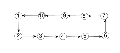
In the first example, we consider a directed circular network. (Fig. 1 shows an example of a circular network with 101010 nodes.) It is obvious that this network is strongly connected. If we assign each edge with weight 111, then the graph Laplacian is

L=[1000001110000001100000011000000110000001100000011]𝐿delimited-[]1000001missing-subexpressionmissing-subexpression1100000missing-subexpressionmissing-subexpression0110000missing-subexpressionmissing-subexpression001missing-subexpressionmissing-subexpression1000missing-subexpressionmissing-subexpression0001100missing-subexpressionmissing-subexpression0000110missing-subexpressionmissing-subexpression0000011missing-subexpressionmissing-subexpression\displaystyle L=\left[\begin{array}[]{cccccccccc}1&0&0&\cdots&0&0&0&-1\\ -1&1&0&\cdots&0&0&0&0\\ 0&-1&1&\cdots&0&0&0&0\\ 0&0&-1&\ddots&\vdots&\vdots&\vdots&\vdots\\ \vdots&\vdots&\vdots&\ddots&1&0&0&0\\ 0&0&0&\cdots&-1&1&0&0\\ 0&0&0&\cdots&0&-1&1&0\\ 0&0&0&\cdots&0&0&-1&1\\ \end{array}\right]

Then we have ξi=0.01subscript𝜉𝑖0.01\xi_{i}=0.01 for each i𝑖i, and λ2=3.9465×10⁵subscript𝜆23.9465superscript105\lambda_{2}=3.9465\times 10^{-5}.

Refer to caption
Figure 1: A circular network consisting of 101010 nodes.

Randomly choose an initial value x(0)𝑥0x(0) whose x¯(0)=0.4886¯𝑥00.4886\bar{x}(0)=0.4886. The objective is to drive the network to reach a consensus on value 00. After calculation, we have

V(0)=0.01i=1100[xi(0)x¯(0)]2=0.5935,𝑉00.01superscriptsubscript𝑖1100superscriptdelimited-[]subscript𝑥𝑖0¯𝑥020.5935V(0)=0.01\sum_{i=1}^{100}[x_{i}(0)-\bar{x}(0)]^{2}=0.5935,
V(0)/x¯2(0)=2.4856.𝑉0superscript¯𝑥202.4856V(0)/\bar{x}^{2}(0)=2.4856.

Let bk=11subscript𝑏𝑘11b_{k}=11 for each k𝑘k, then we can set η1=η2=11subscript𝜂1subscript𝜂211\eta_{1}=\eta_{2}=11. Choose ϵ=0.00999italic-ϵ0.00999\epsilon=0.00999. Then,

C=[2+4η22(1ξ1)]ϵ2/ξ1+4η22ξ1(1ξ1)[1η2(ξ1+ϵ)]2=15.7641.𝐶delimited-[]24superscriptsubscript𝜂221subscript𝜉1superscriptitalic-ϵ2subscript𝜉14superscriptsubscript𝜂22subscript𝜉11subscript𝜉1superscriptdelimited-[]1subscript𝜂2subscript𝜉1italic-ϵ215.7641C=\frac{[2+4\eta_{2}^{2}(1-\xi_{1})]\epsilon^{2}/\xi_{1}+4\eta_{2}^{2}\xi_{1}(1-\xi_{1})}{[1-\eta_{2}(\xi_{1}+\epsilon)]^{2}}=15.7641.

Then we get the lower bound for the duration between each successive impulse is

T=maxi{ξi}λ2lnCξ1ϵ2=1.8662×10³.𝑇subscript𝑖subscript𝜉𝑖subscript𝜆2𝐶subscript𝜉1superscriptitalic-ϵ21.8662superscript103T=\frac{\max_{i}\{\xi_{i}\}}{\lambda_{2}}\ln\frac{C\xi_{1}}{\epsilon^{2}}=1.8662\times 10^{3}.

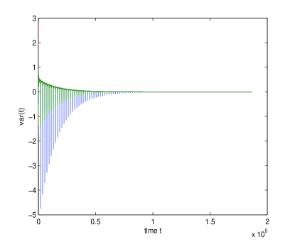
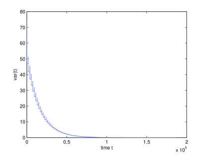
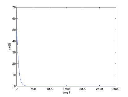
In the simulation, we set Δtk=1867Δsubscript𝑡𝑘1867\Delta t_{k}=1867 for each k𝑘k. The simulation result is presented in Figs.2,3. Fig.2 shows the trajectories of the network, and Fig.3 shows the variations of the trajectories with respect to time t𝑡t which is defined as

var(t)=i=1n|xi(t)|.var𝑡superscriptsubscript𝑖1𝑛subscript𝑥𝑖𝑡\operatorname{\mathrm{var}}(t)=\sum_{i=1}^{n}|x_{i}(t)|.

It can be seen that the network will asymptotically reach a consensus on value 00.

Refer to caption
Figure 2: Pinning consensus to 00 on a circular network with 100100100 nodes.
Refer to caption
Figure 3: The variation of the trajectories of the circular network with 100100100 nodes.

V-B Example 2

In this example, we consider a network that is not strongly connected but has a spanning tree. We start from a circular network with 101010 nodes (shown in Fig.1) and construct a larger network by randomly adding new nodes to the network. At each step, randomly choose a node i𝑖i from the existing network, then a new node j𝑗j is added to the network such that there is a directed edge from i𝑖i to j𝑗j. Continuing this procedure until the network has 100100100 nodes, we obtain a graph that has spanning trees but is not strongly connected. If we assign each edge with weight 111, then in the graph Laplacian (53),

L11=[1000000001110000000001100000000011000000000110000000001100000000011000000000110000000001100000000011]subscript𝐿11delimited-[]1000000001110000000001100000000011000000000110000000001100000000011000000000110000000001100000000011\displaystyle L_{11}=\left[\begin{array}[]{cccccccccc}1&0&0&0&0&0&0&0&0&-1\\ -1&1&0&0&0&0&0&0&0&0\\ 0&-1&1&0&0&0&0&0&0&0\\ 0&0&-1&1&0&0&0&0&0&0\\ 0&0&0&-1&1&0&0&0&0&0\\ 0&0&0&0&-1&1&0&0&0&0\\ 0&0&0&0&0&-1&1&0&0&0\\ 0&0&0&0&0&0&-1&1&0&0\\ 0&0&0&0&0&0&0&-1&1&0\\ 0&0&0&0&0&0&0&0&-1&1\end{array}\right]

Thus ξi=0.1subscript𝜉𝑖0.1\xi_{i}=0.1 for 1i101𝑖101\leq i\leq 10, ξi=0subscript𝜉𝑖0\xi_{i}=0 for 11i10011𝑖10011\leq i\leq 100, and λ2=0.3820subscript𝜆20.3820\lambda_{2}=0.3820. Randomly choose the initial value x(0)𝑥0x(0) where x¯(0)=0.3909¯𝑥00.3909\bar{x}(0)=0.3909. The objective is to drive the network to reach consensus on the value 00. After calculation, we have:

V(0)=i=110ξi[xi(0)x¯(0)]2=0.6369.𝑉0superscriptsubscript𝑖110subscript𝜉𝑖superscriptdelimited-[]subscript𝑥𝑖0¯𝑥020.6369V(0)=\sum_{i=1}^{10}\xi_{i}[x_{i}(0)-\bar{x}(0)]^{2}=0.6369.
V(0)/x¯2(0)=4.1677.𝑉0superscript¯𝑥204.1677V(0)/\bar{x}^{2}(0)=4.1677.

Let bk=5subscript𝑏𝑘5b_{k}=5 for each k𝑘k, then we can set η1=η2=5subscript𝜂1subscript𝜂25\eta_{1}=\eta_{2}=5. Choose ϵ=0.09italic-ϵ0.09\epsilon=0.09. Then we have

C=[2+4η22(1ξ1)]ϵ2/ξ1+4η22ξ1(1ξ1)[1η2(ξ1+ϵ)]2=7.3280.𝐶delimited-[]24superscriptsubscript𝜂221subscript𝜉1superscriptitalic-ϵ2subscript𝜉14superscriptsubscript𝜂22subscript𝜉11subscript𝜉1superscriptdelimited-[]1subscript𝜂2subscript𝜉1italic-ϵ27.3280C=\frac{[2+4\eta_{2}^{2}(1-\xi_{1})]\epsilon^{2}/\xi_{1}+4\eta_{2}^{2}\xi_{1}(1-\xi_{1})}{[1-\eta_{2}(\xi_{1}+\epsilon)]^{2}}=7.3280.

Thus the lower bound for the intervals between each successive impulse is

T=maxi{ξi}λ2lnCξ1ϵ2=14.8720.𝑇subscript𝑖subscript𝜉𝑖subscript𝜆2𝐶subscript𝜉1superscriptitalic-ϵ214.8720T=\frac{\max_{i}\{\xi_{i}\}}{\lambda_{2}}\ln\frac{C\xi_{1}}{\epsilon^{2}}=14.8720.

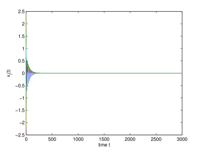
In the simulation, we choose Δtk=15Δsubscript𝑡𝑘15\Delta t_{k}=15. The simulation result is presented in Figs.4, 5. It can be seen that the network will asymptotically reach a consensus on 00.

Refer to caption
Figure 4: Pinning consensus to 00 on the graph that has spanning trees.
Refer to caption
Figure 5: The variation of the trajectories on a graph that has spanning trees.

VI Conclusions

In this paper, we investigate pinning consensus in networks of multiagents via a single impulsive controller. First, we prove a sufficient condition for a network with a strongly connected underlying graph to reach consensus on a given value. Then we extend the result to networks with a spanning tree. Interestingly, we find the permissible range of the impulsive strength is determined by the left eigenvector of the graph Laplacian corresponding to the zero eigenvalue and the pinning node we choose. Besides, a sparse enough impulsive pinning on one node can always drive the network to reach consensus on a prescribed value. Examples with numerical simulations are also provided to illustrate the theoretical results. The pinning synchronization in complex networks via a single impulsive controller is an interesting issue, which will be worked out soon.

References

  • [1] W. Ren, R.W. Beard, and E.M. Atkins, ”A survey of consensus problems in multi-agent coordination”, in Proceedings of 2005 American Control Conference, pp. 1859-1864, 2005.
  • [2] R. Olfati-Saber, ”Consensus and cooperation in networked multi-agent systems”, Proceedings of the IEEE, vol. 95, no. 1, pp. 215-233, 2007.
  • [3] W. Lu, T. Chen, “Synchronization of coupled connected neural networks with delays”, IEEE Transactions on Circuits and Systems-I, Regular Papers, vol. 51, no. 12, pp. 2491-2503, 2004.
  • [4] W. Lu, T. Chen, ”New approach to synchronization analysis of linearly coupled ordinary differential systems”, Physica D, vol. 213, pp. 214-230, 2006.
  • [5] T. Chen, S. Amari, and Q. Lin, ”A unified algorithm for principal and minor component extraction”, Neural Networks, vol. 11, no. 3, pp.385-389, 1998.
  • [6] T. Chen, Y. Hua, and W. Yan, ”Global convergence of oja’s subspace algorithm for principal component extraction”, IEEE Transactions on Neural Networks, vol.8, (1998) pp.57-68
  • [7] T. Chen, X. Liu, and W. Lu, ”Pinning complex networks by a single controller”, IEEE Transactions on Circuits and Systems-I: Regular Papers, vol. 54, no. 6, pp. 1317-1326, 2007.
  • [8] K. Moore, and D. Lucarelli, ”Forced and constrained consensus among cooperating agents”, in IEEE international conference on networking, sensing and control, pp. 449-454, 2005.
  • [9] Z. Yang, and D. Xu, ”Stability analysis of delay neural networks with impulsive effects”, IEEE Transactions on Circuits and Systems II-Express Briefs, vol. 52, no. 8, pp. 517-521, 2005.
  • [10] F. Chen, Z. Chen, L. Xiang, Z. Liu, and Z. Yuan, “Reaching a consensus via pinning control”, Automatica, vol. 45, pp. 1215-1220, 2009.
  • [11] T. Insperger, ”Act-and-wait concept for continuous-time control systems with feedback delay”, IEEE Transactions on Control Systems Technology, vol. 14, no. 5, pp. 974-977, 2006.
  • [12] T. Insperger and G. Stepan, ”Act-and-wait control concept for discrete-time systems with feedback delay”, IET Control Theory and Applications, vol. 1, no. 3, pp. 553-557, 2007.
  • [13] W. Xia and J. Cao, ”Pinning synchronization of delayed dynamical networks via periodically intermittent control”, Chaos, vol. 19, no. 1, 013120, 2009.
  • [14] X. Liu and T. Chen, “Cluster synchronization in directed networks via intermittent pinning control”, IEEE Transactions on Neural Networks, vol. 22, no. 7, pp. 1009-1020, 2011.
  • [15] X. Liu, ”Stability results for impulsive differential systems with applications to population growth models”, Dynamics and Stability of Systems, vol. 9, no. 2, pp. 163-174, 1994.
  • [16] X. Liu, and A. Willms, ”Impulsive controllability of linearly dynamical systems with applications to maneuvers of spacecraft”, Mathematical Problems in Engineering, vol. 2, no. 4, pp. 277-299, 1996.
  • [17] T. Yang, and L. Chua, ”Impulsive stabilization for control and synchronization of chaotic systems: Theory and application to secure communication”, IEEE Transactions on Circuits and Systems I-Foundamental Theory and Applications, vol. 44, no. 10, pp. 976-988, 1997.
  • [18] T. Yang, Impulsive Systems and Control: Theory and Applications. Huntington, NY: Nova Science, 2001.
  • [19] B. Liu, and D. Hill, ”Impulsive consensus for complex dynamical networks with nonidentical nodes and coupling time-delays”, SIAM Journal on Control and Optimization, vol. 49, no. 2, pp. 315-338, 2011.
  • [20] W. Xiong, D. Ho, and Z. Wang, ”Consensus analysis of multiagent networks via aggregated and pinning approaches”, IEEE Transactions on Neural Networks, vol. 22, no. 8, pp. 1231-1240, 2011.
  • [21] J. Zhou, Q. Wu, and L. Xiang, ”Pinning complex delayed dynamical networks by a single impulsive controller”, IEEE Transactions on Circuits and Systems-I: Regular Papers, vol. 58, no. 12, pp. 2882-2893, 2011.
  • [22] J. Lu, J. Kurths, J. Cao, N. Mahdavi, and C. Huang, ”Synchronization control for nonlinear stochastic dynamical networks: pinning impulsive strategy”, IEEE Transactions on Neural Networks and Learning Systems, vol. 23, no. 2, pp. 285-292, 2012.
  • [23] L. Guo, Z. Xu, and M. Hu, ”Projective synchronization in drive-response networks via impulsive control”, Chinese Physics Letters, vol. 25, no. 8, pp. 2816-2819, 2008.
  • [24] Z. Guan, Z. Liu, G. Feng, and Y. Wang, ”Synchronization of complex dynamical networks with time-varying delays via impulsive distributed control”, IEEE Transactions on Circuits and Systems-I: Regular Papers, vol. 57, no. 8, pp. 2182-2195, 2010.
  • [25] Y. Tang, S. Leung, W. Wong, and J. Fang, ”Impulsive pinning synchronization of stochastic discrete-time networks”, Neurocomputing, vol. 73, pp. 2132-2139, 2010.
  • [26] P. DeLellis, M. di Bernardo, and M. Porfiri, ”Pinning control of complex networks via edge snapping”, Chaos, vol. 21, 033119, 2011.
  • [27] H. Su, Z. Rong, M. Chen, X. Wang, G. Chen, and H. Wang, ”Decentralized adaptive pinning control for cluster synchronization of complex dynamical networks”, IEEE Transactions on Systems, Man, and Cybernetics-Part B: Cybernetics, 2012.