How many-body effects modify the van der Waals interaction between graphene sheets

Abstract

Undoped graphene (Gr) sheets at low temperatures are known, via Random Phase Approximation (RPA) calculations, to exhibit unusual van der Waals (vdW) forces. Here we show that graphene is the first known system where effects beyond the RPA make qualitative changes to the vdW force. For large separations, $D\gtrsim 10$nm where only the $\pi_{z}$ vdW forces remain, we find the Gr-Gr vdW interaction is substantially reduced from the RPA prediction. Its $D$ dependence is very sensitive to the form of the long-wavelength many-body enhancement of the velocity of the massless Dirac fermions, and may provide independent confirmation of the latter via direct force measurements.

I Introduction

It is well known that a zero-gap conical $\pi_{z}$ electronic Bloch band structure of undoped graphene, supporting massless Dirac fermions propagating with speed $v$, should give this system a number of unusual properties. Castro Neto et al. (2009) One such property relates to the low-temperature dispersion (van der Waals) interaction energy per unit area $E^{\text{vdW}}/A$ between undoped parallel graphene sheets separated by a large distance $D$. Commonly used theories such as the summation of pairwise atomic contributions, $E^{\text{vdW}}\approx\sum_{i\neq j}C_{ij}R_{ij}^{-6}$, and other popular and largely successful approaches Grimme (2006); Dion et al. (2004); Langreth et al. (2005); Tkatchenko and Scheffler (2009); Vydrov and Van Voorhis (2010), predict the energy for this case (and any case with parallel 2D sheet geometry) to be a power law

$$\frac{E^{\rm vdw}}{A}= -\frac{C_{4}}{D^{4}}$$ (1)

where $C_{4}$ is a system-dependent constant (see Sections 4 and 8 of Ref. Dobson and Gould, 2012 for further discussion). By contrast, more microscopic/collective approaches, such as the RPA correlation energy based on the graphene $\pi_{z}$ -$\pi_{z}^{\ast}$ electronic response, yield the result Dobson et al. (2006); Gould et al. (2008); Sernelius (2012); Gould et al. (2013a); Sharma et al. (2014)

$$\frac{E^{\rm vdw}}{A}= -\frac{C_{3}}{D^{3}}\,.$$ (2)

The constant $C_{3}$ is easily calculated within the random phase approximation (RPA), which treats the electrons in each layer as essentially non-interacting, but subjected to their own time-dependent classical electrostatic field. Indeed, if one makes the simplest (“Casimir-Polder”) approximation, in which the interlayer Coulomb interaction is treated by second-order perturbation theory, one finds, in the limit of large separation

$$C_{3}= \frac{e^{2}}{32\pi}F\left(\frac{\pi}{2}\alpha\right)\,,$$ (3)

where $\alpha=\frac{e^{2}}{\hbar v}$ is the effective fine structure constant of graphene, related to the velocity $v$ of the massless Dirac fermions as the fundamental fine structure constant is to the speed of light, and $F(a)$ is a smoothly varying function, which is plotted in Fig. 1 (the derivation of this result, as well as the analytic expression for $F(a)$ will be presented below).

Figure 1: Plot of the function $F$ which controls, via Eq. (3), the value of the constant $C_{3}$ for the RPA van der Waals interaction between graphene sheets.

For $v=10^{6}$m/s one has $\alpha\simeq 2.2$, which makes $C_{3}$ very close to the “universal” value $C_{3}^{\rm uni}=\frac{e^{2}}{32\pi}$. This value is weakly dependent on small variations of $v$, and remarkably, the interaction $-C_{3}^{\rm uni}/D^{3}$ is not changed by the inclusion of electromagnetic retardation, even at large $D$ values. (see Eq. 36 of Drosdoff and Woods (2010), Drosdoff et al. (2012), and Eq. 8b of [][Note:$χ_0$inthisworkwastoolargebyafactoroftwo]Dobson2006 corrected for a spurious factor 2)

In this context it is important to note that for real graphene Eq. (2) is valid only at large separations: at shorter distances, gapped transitions other than the $\pi_{z}\rightarrow\pi_{z}^{\ast}$ contribute a vdW energy of the conventional form (1). It is only for $D\gtrsim 10\text{nm}$ that numerical work within the RPALebègue et al. (2010) suggests the $D^{-3}$ falloff overtakes the conventional $D^{-4}$ contribution. It is therefore in this regime of larger separations corresponding to small wavevectors that one should check for any many-body effects beyond the RPA due to the $\pi_{z}-\pi_{z}^{\ast}$ graphene response. Furthermore at these separations all electrostatic and metallic overlap forces have long vanished.

II Renormalization of the velocity

Such corrections are worth investigating because the $\pi_{z}$ electrons in a graphene sheet are obviously not “weakly interacting”: the coupling constant $\alpha$ is larger than oneGonzález et al. (1994, 1999); Li et al. (2008); Elias et al. (2011); Siegel et al. (2011). What is believed to be true is that the effective long-wavelength Hamiltonian, generated by a renormalization group (RG) flow, is non-interacting.González et al. (1994, 1999); Herbut (2006); Mishchenko (2009); Kotov et al. (2012) However, the reason for this simplification is not that the electric charge renormalizes to zero but that the fermion velocity grows to infinity. More precisely, if one introduces an effective Fermion velocity $v_{q}$, which describes the system at length scales larger than $1/q$, then $v_{q}\to\infty$ for $q\to 0$, and, accordingly, the running coupling constant $\alpha_{q}=\frac{e^{2}}{\hbar v_{q}}$ tends to zero. This long-wavelength renormalization is quite distinct from beyond-RPA corrections at short wavelength, arising from modified forms of Adiabatic Local Density Functional Theory (ALDA), which are also sometimes also described as ”renormalized”Olsen and Thygesen (2012) Our long-wavelength corrections can change the asymptotic power law for the van der Waals interaction, whereas the short-ranged ALDA-based ones, unsurprisingly, have no major qualitative effect on long-wavelength vdW phenomenaOlsen and Thygesen (2013).

The stronger the original interaction is at the microscopic scale, the larger the renormalized velocity becomes at any given length scale $1/q$. The exact form of the divergence of $v_{q}$ for $q\to 0$ is, of course, unknown, since the many-body problem has not been solved. RG calculations based on first-order perturbation theory González et al. (1994); Kotov et al. (2012) suggest a weak logarithmic divergence of the form

$$v^{(1)}_{q}= v\left(1+\frac{1}{4}\alpha\ln\frac{\Lambda}{q}\right)\,, \alpha_{q}^{(1)}= \frac{\alpha}{1+\frac{1}{4}\alpha\ln\frac{\Lambda}{q}}\,,$$ (4)

where $\Lambda$ is a microscopic cutoff of the order of the inverse of the lattice constant (Å). More sophisticated calculations at the “two-loop” level and in the large-$N$ limit, González et al. (1999); Polini et al. (2007); Das Sarma et al. (2007); Son (2007); Foster and Aleiner (2008); Kotov et al. (2009, 2012) $N$ being the number of Fermion flavors, predict a stronger power-law divergence of the form

$$v^{(2)}_{q}= v\left(\frac{\Lambda}{q}\right)^{\beta}\,, \alpha_{q}^{(2)}= \frac{\alpha}{\left(\Lambda/q\right)^{\beta}}\,,$$ (5)

where $\beta=\frac{8}{N\pi^{2}}$, ($N=4$ for graphene). Recent experiments performed by a variety of techniques have at least partially confirmed these theoretical predictionsLi et al. (2008); Reed et al. (2010); Elias et al. (2011); Siegel et al. (2011), showing that the effective coupling constant is reduced and the Dirac cones are strongly compressed Elias et al. (2011) near the Dirac point.

The many-body enhancement of the fermion velocity has also been shown to affect various many-body phenomena, such as the plasmon dispersion Abedinpour et al. (2011); Levitov et al. (2013), the optical Drude weight, Abedinpour et al. (2011) and the electronic screening of external charges.Sodemann and Fogler (2012) To dateOlsen and Thygesen (2012, 2013), beyond-RPA effects were believed to alter at most the prefactor, not the power exponent, of vdW decay with distance. In this Letter we expose a striking case where beyond-RPA many-body renormalization affects the essential character of a vdW interaction, namely that between graphene sheets. Our main result is that the long-wavelength enhancement of the fermion velocity causes the vdW interaction to decrease asymptotically faster than in Eq. (2) but still slower than in the conventional Eq. (1). This result can be expressed in an intuitively appealing way by saying that the bare $\alpha$ in Eq. (3) must be replaced by the running coupling constant $\alpha_{q}$ evaluated at $q=1/D$. Thus we have

$$\frac{E^{\rm vdw}}{A}\simeq-\frac{e^{2}}{32\pi D^{3}}F\left(\frac{\pi}{2}\alpha_{1/D}\right)\,,$$ (6)

and since $F(x)\simeq\frac{\pi}{2}x$ for $x\ll 1$ the asymptotic behavior of the vdW interaction is reduced, relative to the RPA, precisely by the factor $\alpha_{1/D}$, which vanishes in the limit $D\to\infty$. The renormalized interaction will therefore decrease as $[D^{3}\ln(D\Lambda)]^{-1}$ or as $D^{-(3+\beta)}$, depending on which of the two scenarios, (4) or (5), is realized. Additional many-body effects contained in the so-called vertex corrections turn out to be irrelevant at sufficiently large distance, even though, of course, they can quantitatively change the result at intermediate distances. Throughout the analysis, we assume that the distances are not so large that $v_{q=1/(2D)}$ becomes comparable to the speed of light, at which point electromagnetic retardation effects should be taken into account. Using this criterion, retardation becomes dominant only for $D$ of order $10^{220}$m (!) for the logarithmic renormalization case [Eq. (4)] or $O(10^{1}\text{m})$ for the power law case [Eq. (4)]. Thus retardation here is unimportant in practice, as for the pure RPA theory.

III van der Waals Calculations

We consider the interaction energy between two parallel freely suspended graphene sheets in vacuo, separated by a distance $D$ that is much larger than the two-dimensional lattice constant $a$, as well as the thickness $T$ of each sheet (see Appendix A for other scenarios). Our starting point is the Casimir-Polder (CP) formula obtained by doing straightforward second-order perturbation theory in the inter-layer electron-electron interaction potential

$$V_{\rm inter}(q)= \frac{2\pi e^{2}}{q}e^{-qD}\,,$$ (7)

where ${\bf q}$ is the two-dimensional wave vector of density fluctuations in each layer. The result is

$$\frac{E^{(2)}}{A}= \frac{-\hbar}{8\pi^{3}}\int_{0}^{\infty}\text{d}u\int d^{2}{\bf q}\chi(q,iu)^{2}\left(\frac{2\pi e^{2}}{q}e^{-qD}\,.\right)^{2}$$ (8)

Here $\chi(q,iu)$ is the electronic density-density response function of a single isolated layer, evaluated at wave vector ${\bf q}$ and imaginary frequency $iu$. The exponentially decaying factor $\exp(-2qD)$ ensures that small wave vectors $q\approx 1/D$ dominate Eq. (8) for large separations.

The response function $\chi(q,iu)$ is expressed in terms of the proper response function $\tilde{\chi}(q,iu)$ and the intra-layer interaction potential $V_{\rm intra}(q)=\frac{2\pi e^{2}}{q}$ according to the well-known formula Giuliani and Vignale (2005)

$$\chi(q,iu)= \frac{\tilde{\chi}(q,iu)}{1-\frac{2\pi e^{2}}{q}\tilde{\chi}(q,iu)}$$ (9)

In the RPA one approximates $\tilde{\chi}(q,iu)\approx\chi_{0}(q,iu)$, where

$$\chi_{0}(q,iu)=-\frac{1}{4\hbar v}\frac{q}{\sqrt{1+x^{2}}}\,,$$ (10)

is the non-interacting zero-temperature response function for the conical $\pi_{z}-$bands,González et al. (1994); Wunsch et al. (2006); Dobson et al. (2006) $v$ is the bare velocity, and $x\equiv\frac{u}{qv}$.

Intra-layer electron-electron interactions modify $\tilde{\chi}$ in two ways: via self-energy insertions and via vertex corrections. For example, in a recent first-order perturbative calculation coupled with RG arguments, Sodemann and Fogler (SF) findSodemann and Fogler (2012)

$$\tilde{\chi}(q,iu)= -\frac{q}{4\hbar v_{q}}\left(\frac{1}{\sqrt{x^{2}+1}}+\alpha_{q}J(x)\right)\,,$$ (11)

where $v_{q}$ is given by Eq. (4) (i.e., $v_{q}=v_{q}^{(1)}$) and $\alpha_{q}$ is the corresponding coupling constant. Here the self-energy insertion has caused the bare velocity $v$ to be replaced by the renormalized, scale-dependent velocity $v_{q}$. The second term, $J$, is a dimensionless function representing the combined effects of self-energy and vertex corrections beyond the simple rescaling of $v$. In the notation of SF $J$ is given by $J(x)\equiv I_{a}(ix)+I_{b}(ix)$ where the functions $I_{a}$ and $I_{b}$, defined in Ref. Sodemann and Fogler, 2012, are analytically continued here to the imaginary $x$ axis. It is essential to our subsequent arguments that $J(x)$ is a smooth function of $x$, varying monotonically between $J(0)\approx 0.497$ and $J(x\to\infty)\approx\frac{0.013}{x}\equiv\frac{C_{\infty}}{x}$ (see Eq. (12) and Fig. 2, where a numerical fit to $J(x)$ is provided).

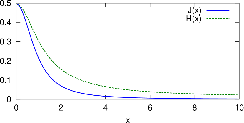
Figure 2: (Color online) Numerical fit [Eq. (12)] to the functions $J(x)$ (solid line) and $H(x)\equiv J(x)\sqrt{1+x^{2}}$ (dashed line) which control the magnitude of the self-energy and vertex corrections to the RPA beyond the simple renormalization of the velocity.

This feature is expected to persist beyond the first-order approximation, e.g., even in the strong coupling limit, where the renormalized velocity is likely given by $v^{(2)}_{q}$ of Eq. (5) (see Ref. Kotov et al., 2012). A simple fit to $J(x)$ based on the results of Ref. Sodemann and Fogler, 2012 is

$$J(x)= \frac{(y+a)J(0)+(y^{3}-1)aC_{\infty}}{y^{3}(1+ay)}\,,$$ (12)

where $a=0.285$ and $y=\sqrt{1+x^{2}}$. This is shown in Fig. 2. For imaginary $x$, this numerical fit provides a good match to the results of Ref. Sodemann and Fogler, 2012.

Substituting Eq. (11) into Eq. (9) we obtain the full interacting response function in the form

$$\chi(q,iu)= -\frac{q}{4\hbar v}\frac{1+\alpha_{q}H(x)}{\sqrt{1+x^{2}}+\frac{\pi}{2}\alpha_{q}[1+\alpha_{q}H(x)]}\,,$$ (13)

where $H(x)\equiv J(x)\sqrt{1+x^{2}}$. Plugging into Eq. (8) and changing integration variable from $q$ to $\bar{q}=2qD$ we find, after simple manipulations

$$\frac{E^{(2)}}{A}=-\frac{e^{2}}{32\pi D^{3}}\int_{0}^{\infty}\frac{1}{2}\bar{q}^{2}e^{-\bar{q}}\tilde{F}\left(\frac{\pi}{2}\alpha_{\bar{q}/2D}\right)\text{d}\bar{q}\,,$$ (14)

where we have defined the function

$$\tilde{F}(a)\equiv a\int_{0}^{\infty}\left\{\frac{1+\frac{2a}{\pi}H(x)}{\sqrt{1+x^{2}}+a[1+\frac{2a}{\pi}H(x)]}\right\}^{2}\text{d}x\,.$$ (15)

If now self-energy and vertex corrections are neglected by setting $H=0$, we see that $\tilde{F}$ simplifies to

$$F(a)\equiv a\int_{0}^{\infty}\left\{\frac{1}{\sqrt{1+x^{2}}+a}\right\}^{2}\text{d}x\,,$$ (16)

which can be evaluated analytically, yielding

$$F(a)= \begin{cases}\frac{\frac{a\pi}{2}-a^{2}\sqrt{1-a^{2}}-a\tan^{-1}\left(\frac{a}{\sqrt{1-a^{2}}}\right)}{(1-a^{2})^{3/2}},&a<1\\ \frac{a^{2}-\frac{a}{2\sqrt{a^{2}-1}}\log\frac{a+\sqrt{a^{2}-1}}{a-\sqrt{a^{2}-1}}}{(a^{2}-1)}\,,&a>1\end{cases}$$ (17)

and $F(a)=2/3$ for $a=1$. This is precisely the function $F$ that was introduced in Eq. (3) and was plotted in Fig. (1). Since in RPA $\alpha_{q}$ is constant ($\alpha_{q}=\alpha$) and $\int_{0}^{\infty}\bar{q}^{2}e^{-\bar{q}}\text{d}\bar{q}=2$, Eq. (3) is seen to follow immediately from Eq. (14).

To go beyond the RPA we must reinstate the self-energy and the vertex corrections. However, we observe that in the large-$D$ limit the coupling constant tends to zero and therefore the $\tilde{F}$ function reduces to the $F$ function, which in turn can be replaced by its small-$a$ expansion $F(a)\approx\frac{\pi}{2}a$. Thus, Eq. (14) becomes

$$\frac{E^{(2)}}{A}= -\frac{\pi e^{2}}{256D^{3}}\int_{0}^{\infty}\bar{q}^{2}e^{-\bar{q}}\alpha_{\bar{q}/2D}\text{d}\bar{q}\,,$$ (18)

The asymptotic behavior of the vdW interaction depends solely on the behavior of the running coupling constant $\alpha_{q}$ (or, equivalently, the renormalized velocity) in the $q\to 0$ limit. For the logarithmic renormalization case of Eq. (4), we evaluate (18) by freezing the slowly varying $\alpha_{q/2D}^{(1)}$, evaluating it at the maximizing value $q_{0}=2$ of the rapidly varying integrand, getting

$$\frac{E^{(2)}}{A}\approx -\frac{\pi e^{2}}{128D^{3}}\left[\frac{\alpha}{1+\frac{1}{4}\alpha\ln(\Lambda D)}\right]\,.$$ (19)

This shows a modest, logarithmic reduction of the vdW interaction relative to the RPA result. If, on the other hand, the strong-coupling model of Eq. (5) is adopted, (18) gives an altogether different power-law behavior:

$$\frac{E^{(2)}}{A}=-\frac{\pi\Gamma(3+\beta)\Lambda^{\beta}e^{2}}{32(2D)^{3+\beta}}\,,$$ (20)

where $\Gamma(x)$ is the gamma function. Notice that, since $\beta<1$, this is still larger than the $D^{-4}$ dependence expected for insulating 2D layers, and therefore dominates at large separations in real graphene where gapped insulator type transitions also contribute to the response.

The above eqs. (18-20) are valid at asymptotically large separations. At finite separations the more accurate Eqs (14)-(15) must be used. These now depend not only on the fermion velocity – a measurable quantity – but also on the form of the function $J(x)$, which is not directly accessible to experiment and must be calculated by many-body theory (Notice, however, that the imaginary part of the density response function for real frequency is related to the optical absorption spectrum, which is, in principle, measurable, and could be used to calculate the function $J$). Making use of $J(x)$ calculated in Ref. Sodemann and Fogler, 2012 and fitted as shown in Fig. 2 we find that

$$\tilde{F}(a)\approx\left(1+0.165\frac{(2.1a)}{\sqrt{1+(2.1a)^{2}}}\right)F(a)$$ (21)

is an excellent approximation (relative error under 1%) to the integral of Eq. (15).

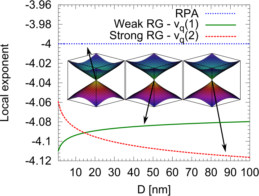
Figure 3: Plot of the local exponent $\frac{d\log{|F|}}{d\log{D}}$ of the force (top, with bandstructure inset) and the force $F=\frac{dE^{(2)}}{dD}$ (bottom) using RPA [dotted line], $v_{q}^{(1)}$ [Eq. (4), solid line] and $v_{q}^{(2)}$ [Eq. (5) with $\beta=2/\pi^{2}$, dashed line]. Here we fix $v=10^{5}$m/s and $\Lambda=1/(1.42{\text{\AA}})$.

Using this in Eq. (14), together with Eq. (4) or (5) for the velocity, we find that the distance dependence in the intermediate regime is basically $D^{-3}$ with only a modest further dependence on distance via $F\left(\frac{\pi}{2}\alpha_{q=1/D}\right)$ or $\tilde{F}\left(\frac{\pi}{2}\alpha_{q=1/D}\right)$.

In Fig. 3 we plot the force and its local exponent [in $F\propto D^{-p(D)}$] for the RPA energy $E^{(2)}_{\text{RPA}}/A=-e^{2}/(32\pi D^{3})F(\alpha)$ and the vdW interaction calculated through (14) using (4) and (5). Using the stretched graphite vdW energy formula of Refs. Gould et al., 2009, 2013a yields remarkably similar results for the equivalent in bulk graphite (up to a constant). Naturally, the situation differs between the weak-coupling (4) and strong-coupling (5) models of the renormalized velocity. The interaction energy and force is qualitatively different from RPA at large separations, and shows moderate quantitative differences at intermediate separations, less than 25% for $D<100$Å. Observation of such deviations from the RPA will provide additional evidence of the many-body renormalization of the fermion velocity. We note that for intermediate values of $D$ ($D\lesssim 20$nm), further modifications are required even at the RPA level to account for departures of the graphene electronic bandstructure from a perfect infinite coneGould et al. (2013a), or anisotropySharma et al. (2014).

There have been some proposals (Kotov et al. (2012) and references therein) that strong coupling could bring excitonic effects leading to a gap. In that case the vdW energy might show the insulating $D^{-4}$ behavior as in Eq (1). There seems to be little experimental evidence so far that graphene can be an excitonic insulator, however.

IV Experimental options

While our paper in the main concerns the theory of the renormalization of the vdW interaction, it serves as one of several motivating factors for a renewed experimental effort for direct measurement of the vdW forces on high-quality graphene flakes. These measurements would also be needed to resolve existing controversies about graphitic cohesion in general. In this section we briefly discuss the current prospects for such measurements, and we hope thereby to stimulate experimentalists in this direction.

While there have been a number of experimentsGirifalco and Lad (1956); Benedict et al. (1998); Zacharia et al. (2004); Liu et al. (2012) that have indirectly determined the binding energy of graphene planes, these have produced a wide range of results, and most have relied on questionable theoretical assumptions for their analysis, so that the whole field is somewhat controversialGould et al. (2013b). Purely theoretical estimates have also varied widelyDion et al. (2004); Hasegawa and Nishidate (2004); Chakarova-Käck et al. (2006); Ziambaras et al. (2007); Hasegawa et al. (2007); Spanu et al. (2009); Lebègue et al. (2010); Drosdoff and Woods (2010); Thrower et al. (2013); Bučko et al. (2013), though recent very large and relatively high-level (RPALebègue et al. (2010), DMCSpanu et al. (2009)) calculations are starting to show consistency. These same high-level types of theory also predict the forces between nanostructures such as graphene planes as a function of distance, showing very different results from popular pairwise-additive-force theories, in the asymptotic region of large separations [see Eqs (2), (6)].

The force between graphenes at such asymptotic distances does not appear to have been measured at all so far. In view of this, as well as the aforementioned binding-energy controversies, direct measurement of such forces at all distances would be very desirable. As the distant forces are relatively small, Atomic Force Microscopy or a related NEMS oscillator approach would be the preferred route. For the basic RPA analysis of two cold undoped graphene sheets of lateral dimension 1 micron, separated by 10 nm, the predicted force is a few nanoNewton, well within AFM capabilities, with larger forces for larger flake areas.

In the ideal case analyzed in the main text there are two undoped, freestanding graphene sheets at a temperature below 10K. Single sheets of high-quality graphene have certainly been subjected to various measurementsKnox et al. (2011) and vdW forces due to a single supported graphene sheet has been seenBanishev et al. (2013), but force experiments with two freestanding sheets are rare or absent, and will require some effort to ensure a reasonable degree of parallelism.

Perhaps a better short-term prospect is therefore to measure the force between a single freestanding sheet and its own “vdW image” in the surface of a bulk metallic substrate. A very recent related experiment, using a metal grating instead of graphene, and an $O(100{\mu}\text{m})$-radius gold sphere as the substrate to avoid parallellism issues, have been highly successfulIntravaia et al. (2013). This experiment also demonstrated the use of co-located fiber optics for precise control of the separation $D$ down to $<200$nm. The theory of this geometry will be analyzed in detail elsewhere, but is expected [see equation (28)] to yield similar predictions to the ones in the main text.

The unavoidable corrugation of the freestanding graphene sheets should not be a problem, as it is known experimentally not to affect electronic properties substantially, and would only contribute a very few percent uncertainty in the separation $D$ between the sheets, at the separations of a few tens to hundreds of nanometers that are relevant to the main text. This uncertainty would not affect the analysis of the force power law proposed in the text, as one would aim for measurements at $D$ values spanning an order of magnitude.

A more subtle problem is the likely existence of metallic n- and p-type “puddles” on the undoped sheetsCheng et al. (2011). Provided that the sheets are of sufficient quality that the puddles are disconnected objects of typical spatial extent $\lambda$, we predict that they contribute an “insulator-like” vdW interaction energy varying with distance $D$ as (const)$D^{-4}$ when $D>\lambda$, clearly distinguishable from the lower powers predicted in the text, arising from the un-doped non-puddle areas. Recent experimentsCheng et al. (2011) suggest that $\lambda=O(1\text{nm})$, so that force experiments at $D=O(10\mbox{--}200\text{nm})$ would still exhibit undoped-graphene properties.

Another experimental route would be to avoid separating the sheets in their perpendicular direction, but rather to slide them off one another in a surface-parallel direction. This may be easier experimentally because of the recent centrifugation-based preparation of high-quality micron-sized stacks of $2\mbox{--}5$ graphene monolayersChen et al. (2012). These are spatially staggered like a slipped deck of cards, potentially allowing attachment of an AFM tip to the projecting edges of individual sheets. The force during the entire lateral sliding process, out to wide separation into disjunct coplanar sheets, would be measured. The non-contact part of this force can be expected to show effects from the coupling of long-wavelength electronic charge fluctuations and hence renormalization effects in the graphene polarizability, just as for the case of parallel sheets separated by distance $D$ measured perpendicular to the sheets. From the theory point view, the analysis of this geometry is more difficult and has not yet been attempted in detail.

The above considerations suggest that it will be possible to achieve a much improved understanding of graphenic cohesive forces by direct measurement.

V Conclusion

In conclusion, we have shown that the low-temperature dispersion (vdW) interaction between two infinite parallel non-doped graphene sheets is significantly modified by many-body effects beyond the RPA. Not only is the interaction quantitatively reduced, but also its qualitative asymptotic behavior is modified. The main source of the effect is the many-body renormalization of the velocity of the massless Dirac Fermions. This renormalization has been the subject of many recent investigationsGonzález et al. (1994, 1999); Li et al. (2008); Elias et al. (2011); Siegel et al. (2011). It is experimentally observed as a deformation of the Dirac cones near the point of contact. Our findings demonstrate that the same renormalization manifests itself in the long-distance behavior of the dispersion forces.

Direct measurement of the asymptotic graphene-graphene vdW interaction could therefore distinguish between much-debated theory models of electrons in graphene – weak renormalization [Eq. (19)], strong renormalization [Eq. (20)] and excitonic insulator [Eq. (1)]. Such experiments in the asymptotic vdW region will be demanding but we estimate (e.g.) a measurable force of order nN (see inset of Figure 3) between micron-sized graphene sheets separated by $O(10\text{nm})$. Observation of the vdW image force in a metal substrate could avoid the need for two graphene sheets, and there are other possibilities too (see Ref. Chen et al. (2012) and second last paragraph of Section IV above). Very recent experimentsIntravaia et al. (2013) support the general feasibility of our proposals. We estimate that complications due to graphene wrinkling and puddlingCheng et al. (2011) will not destroy our effect. Indeed the time is ripe for direct force measurements to clarify this and other recent controversiesGould et al. (2013b) over graphenic cohesion in general.

Appendix A van der Waals force between graphene and a metal bulk

Here we investigate the van der Waals force between a single graphene layer and a metal bulk, which may be more appropriate for likely successful experimental arrangements (see Sec. IV below). We predict that it will obey the same overall power law as the response between two graphene layers, with at most a logarithmic correction (as a function of $D$). Similarly the dependence on the many-body beyond-RPA effects is expected to be maintained. Here we offer evidence that this is indeed the case.

We make use of the relationshipDobson (2009)

$$\frac{E_{\text{vdW}}}{A}= \frac{\hbar}{8\pi^{3}}\int\text{d}^{2}\vec{q}\int_{0}^{\infty}\text{d}u\log(1-\zeta)$$ (22)

$$\approx -\frac{\hbar}{8\pi^{3}}\int\text{d}^{2}\vec{q}\int_{0}^{\infty}\text{d}u\zeta$$ (23)

for the van der Waals potential between semi-infinite bulks and layers interacting across a single surface. In the case of a layer of graphene interacting with a bulk metal

$$\zeta= e^{-2qD}\frac{2\pi e^{2}}{q}\chi_{\text{Gr}}(q,iu)$$

$$\times\frac{2\pi e^{2}}{q}\int\text{d}z\text{d}z^{\prime}e^{-q|z+z^{\prime}|}\chi_{\text{Metal}}(q,z,z^{\prime},iu)$$ (24)

$$\equiv C_{\text{Gr}}(q,iu)C_{\text{Metal}}(iu)e^{-2qD}$$ (25)

where $\chi_{\text{Gr}}(q,iu)$ is the interacting response of the graphene layer and $\chi_{\text{Metal}}$ is the bulk response of the metal. Here $C_{\text{Metal}}=\frac{\epsilon(iu)-1}{\epsilon(iu)+1}$ where $\epsilon\approx 1+\frac{\omega_{p}^{2}}{u^{2}}$ is the dielectric function of the metal.

From equations (9) and (13) we see that $C_{\text{Gr}}\equiv\frac{-2\pi e^{2}}{q}\chi_{\text{Gr}}(q,iu)$ can be written as $C_{\text{Gr}}(x,\alpha_{q})\approx\frac{\pi\alpha_{q}/2}{\sqrt{1+x^{2}}+\pi\alpha_{q}/2}$ where $x=u/(v_{q}q)$ and $\alpha_{q}=e^{2}/(\hbar v_{q})$ varies slowly with $q$. Thus

$$\frac{E_{\text{vdW}}}{A}= \frac{e^{2}}{4\pi^{2}D^{3}}\int\bar{q}^{2}e^{-\bar{q}}\text{d}\bar{q}\int_{0}^{\infty}\text{d}x$$

$$\times\frac{C_{\text{Gr}}(x,\alpha_{\bar{q}/(2D)})}{\alpha_{\bar{q}(2D)}}\frac{1}{1+\frac{v^{2}_{\bar{q}/(2D)}\bar{q}^{2}}{2D^{2}\omega_{p}^{2}}x^{2}}$$ (26)

where we also used $\bar{q}=2qD$. Clearly the form of $\alpha_{q}$ will have a substantial effect on the asymptotic behaviour of the vdW potential, similar to the bigraphene case. Using $C_{\text{Gr}}<\frac{\pi/2\alpha}{x+\pi/2\alpha}$ and setting $\alpha_{\frac{\bar{q}}{2D}}\approx\alpha_{1/D}$ gives

$$\frac{E_{\text{vdW}}}{A}< \frac{e^{2}}{4\pi^{2}D^{3}}\int\bar{q}^{2}e^{-\bar{q}}\text{d}\bar{q}\int_{0}^{\infty}\text{d}x$$

$$\times\frac{\pi/2}{x+\pi/2\alpha_{1/D}}\frac{1}{1+\frac{v^{2}_{1/D}\bar{q}^{2}}{2D^{2}\omega_{p}^{2}}x^{2}}$$ (27)

$$\approx \frac{\alpha_{1/D}\log(D/D_{0})}{D^{3}}$$ (28)

where $D_{0}\propto\frac{e^{2}}{\hbar\omega_{p}}=O(1\text{\AA})$ i.e. the asymptotic interaction has an extra logarithmic term compared to the bigraphene case $k\alpha_{1/D}/D^{3}$. The prefactor $\alpha_{1/D}$ ensures that the difference between different renormalization scenarios is maintained.

One can, of course, perform the integral (26) [or an equivalent expression for (22)] numerically for a given graphene velocity $v_{q}$ and dielectric frequency $\omega_{p}$. However, the important asymptotic physics are clearer in the bigraphene case tested in the paper, and the deviation caused by the bulk metal is expected to be small at the $O(10\text{--}100\text{nm})$ distances we propose investigating.

References

- Castro Neto et al. (2009) A. H. Castro Neto, F. Guinea, N. M. R. Peres, K. S. Novoselov, and A. K. Geim, “The electronic properties of graphene,” Rev. Mod. Phys. 81, 109–162 (2009).
- Grimme (2006) Stefan Grimme, “Semiempirical gga-type density functional constructed with a long-range dispersion correction,” J. Comp. Chem. 27, 1787–1799 (2006).
- Dion et al. (2004) M. Dion, H. Rydberg, E. Schröder, D. C. Langreth, and B. I. Lundqvist, “Van der waals density functional for general geometries,” Phys. Rev. Lett. 92, 246401 (2004).
- Langreth et al. (2005) D. C. Langreth, M. Dion, H. Rydberg, E. Schr der, P. Hyldgaard, and B. I. Lundqvist, “Van der waals density functional theory with applications,” Int. J. Quantum Chem. 101, 599–610 (2005).
- Tkatchenko and Scheffler (2009) Alexandre Tkatchenko and Matthias Scheffler, “Accurate molecular van der waals interactions from ground-state electron density and free-atom reference data,” Phys. Rev. Lett. 102, 073005 (2009).
- Vydrov and Van Voorhis (2010) Oleg A. Vydrov and Troy Van Voorhis, “Dispersion interactions from a local polarizability model,” Phys. Rev. A 81, 062708 (2010).
- Dobson and Gould (2012) John F. Dobson and Tim Gould, “Calculation of dispersion energies,” Journal of Physics: Condensed Matter 24, 073201 (2012).
- Dobson et al. (2006) John F. Dobson, Angela White, and Angel Rubio, “Asymptotics of the dispersion interaction: analytic benchmarks for van der Waals energy functionals,” Phys. Rev. Lett. 96, 073201 (2006).
- Gould et al. (2008) Tim Gould, Ken Simpkins, and John F. Dobson, “Theoretical and semiempirical correction to the long-range dispersion power law of stretched graphite,” Phys. Rev. B 77, 165134 (2008).
- Sernelius (2012) Bo E. Sernelius, “Graphene as a strictly 2D sheet or as a film of small but finite thickness,” Graphene 01, 21–25 (2012).
- Gould et al. (2013a) Tim Gould, John F. Dobson, and S. Lebègue, “Effects of a finite dirac cone on the dispersion properties of graphite,” Phys. Rev. B 87, 165422 (2013a).
- Sharma et al. (2014) A. Sharma, P. Harnish, A. Sylvester, V. N. Kotov, and A. H. Castro Neto, “Van der Waals forces and electron-electron interactions in two strained graphene layers,” ArXiv e-prints (2014), arXiv:1402.3369 [cond-mat.mtrl-sci] .
- Drosdoff and Woods (2010) D. Drosdoff and Lilia M. Woods, “Casimir forces and graphene sheets,” Phys. Rev. B 82, 155459 (2010).
- Drosdoff et al. (2012) D. Drosdoff, A.D. Phan, L.M. Woods, I.V. Bondarev, and J.F. Dobson, “Effects of spatial dispersion on the casimir force between graphene sheets,” The European Physical Journal B 85, 1–6 (2012).
- Lebègue et al. (2010) S. Lebègue, J. Harl, Tim Gould, J. G. Ángyán, G. Kresse, and J. F. Dobson, “Cohesive properties and asymptotics of the dispersion interaction in graphite by the random phase approximation,” Phys. Rev. Lett. 105, 196401 (2010).
- González et al. (1994) J. González, F. Guinea, and M.A.H. Vozmediano, “Non-fermi liquid behavior of electrons in the half-filled honeycomb lattice (a renormalization group approach),” Nuclear Physics B 424, 595 – 618 (1994).
- González et al. (1999) J. González, F. Guinea, and M. A. H. Vozmediano, “Marginal-fermi-liquid behavior from two-dimensional coulomb interaction,” Phys. Rev. B 59, R2474–R2477 (1999).
- Li et al. (2008) Z. Q. Li, E. A. Henriksen, Z. Jiang, Z. Hao, M. C. Martin, P. Kim, H. L. Stormer, and D. N. Basov, “Dirac charge dynamics in graphene by infrared spectroscopy,” Nat Phys 4, 532–535 (2008).
- Elias et al. (2011) D. C. Elias, R. V. Gorbachev, A. S. Mayorov, S. V. Morozov, A. A. Zhukov, P. Blake, L. A. Ponomarenko, I. V. Grigorieva, K. S. Novoselov, F. Guinea, and A. K. Geim, “Dirac cones reshaped by interaction effects in suspended graphene,” Nat Phys 7, 701–704 (2011).
- Siegel et al. (2011) David A. Siegel, Cheol-Hwan Park, Choongyu Hwang, Jack Deslippe, Alexei V. Fedorov, Steven G. Louie, and Alessandra Lanzara, “Many-body interactions in quasi-freestanding graphene,” Proceedings of the National Academy of Sciences 108, 11365–11369 (2011).
- Herbut (2006) Igor F. Herbut, “Interactions and phase transitions on graphene’s honeycomb lattice,” Phys. Rev. Lett. 97, 146401 (2006).
- Mishchenko (2009) E. G. Mishchenko, “Dynamic conductivity in graphene beyond linear response,” Phys. Rev. Lett. 103, 246802 (2009).
- Kotov et al. (2012) Valeri N. Kotov, Bruno Uchoa, Vitor M. Pereira, F. Guinea, and A. H. Castro Neto, “Electron-electron interactions in graphene: Current status and perspectives,” Rev. Mod. Phys. 84, 1067–1125 (2012).
- Olsen and Thygesen (2012) Thomas Olsen and Kristian S. Thygesen, “Extending the random-phase approximation for electronic correlation energies: The renormalized adiabatic local density approximation,” Phys. Rev. B 86, 081103 (2012).
- Olsen and Thygesen (2013) Thomas Olsen and Kristian S. Thygesen, “Beyond the random phase approximation: Improved description of short range correlation by a renormalized adiabatic local density approximation,” arXiv abs/1306.2732 (2013).
- Polini et al. (2007) M. Polini, R. Asgari, Y. Barlas, T. Pereg-Barnea, and A. H. MacDonald, “Graphene: A pseudochiral fermi liquid,” Solid State Comm. 143, 58–62 (2007).
- Das Sarma et al. (2007) S. Das Sarma, E. H. Hwang, and Wang-Kong Tse, “Many-body interaction effects in doped and undoped graphene: Fermi liquid versus non-fermi liquid,” Phys. Rev. B 75, 121406 (2007).
- Son (2007) D. T. Son, “Quantum critical point in graphene approached in the limit of infinitely strong coulomb interaction,” Phys. Rev. B 75, 235423 (2007).
- Foster and Aleiner (2008) Matthew S. Foster and Igor L. Aleiner, “Graphene via large : A renormalization group study,” Phys. Rev. B 77, 195413 (2008).
- Kotov et al. (2009) Valeri N. Kotov, Bruno Uchoa, and A. H. Castro Neto, “ expansion in correlated graphene,” Phys. Rev. B 80, 165424 (2009).
- Reed et al. (2010) James P. Reed, Bruno Uchoa, Young Il Joe, Yu Gan, Diego Casa, Eduardo Fradkin, and Peter Abbamonte, “The effective fine-structure constant of freestanding graphene measured in graphite,” Science 330, 805–808 (2010).
- Abedinpour et al. (2011) Saeed H. Abedinpour, G. Vignale, A. Principi, Marco Polini, Wang-Kong Tse, and A. H. MacDonald, “Drude weight, plasmon dispersion, and ac conductivity in doped graphene sheets,” Phys. Rev. B 84, 045429 (2011).
- Levitov et al. (2013) L. S. Levitov, A. V. Shtyk, and M. V. Feigelman, “Electron-electron interactions and plasmon dispersion in graphene,” arXiv:1302.5036 (2013).
- Sodemann and Fogler (2012) I. Sodemann and M. M. Fogler, “Interaction corrections to the polarization function of graphene,” Phys. Rev. B 86, 115408 (2012).
- Giuliani and Vignale (2005) G. F. Giuliani and G. Vignale, Quantum Theory of the Electron Liquid (Cambridge University Press, UK, 2005).
- Wunsch et al. (2006) B Wunsch, T Stauber, F Sols, and F Guinea, “Dynamical polarization of graphene at finite doping,” New J. Phys. 8, 318 (2006).
- Note (1) Some care must be exerted when evaluating Eq. (14\@@italiccorr) as the asymptotic renormalised perturbation approach for the corrections is not fully appropriate for larger . In particular expression (4\@@italiccorr) is invalid for large as can become negative. In our calculations we use instead to avoid unphysical results.
- Gould et al. (2009) Tim Gould, Evan Gray, and John F. Dobson, “van der waals dispersion power laws for cleavage, exfoliation, and stretching in multiscale, layered systems,” Phys. Rev. B 79, 113402 (2009).
- Girifalco and Lad (1956) L. A. Girifalco and R. A. Lad, “Energy of cohesion, compressibility, and the potential energy functions of the graphite system,” The Journal of Chemical Physics 25, 693–697 (1956).
- Benedict et al. (1998) Lorin X. Benedict, Nasreen G. Chopra, Marvin L. Cohen, A. Zettl, Steven G. Louie, and Vincent H. Crespi, “Microscopic determination of the interlayer binding energy in graphite,” Chem. Phys. Letters 286, 490–496 (1998).
- Zacharia et al. (2004) Renju Zacharia, Hendrik Ulbricht, and Tobias Hertel, “Interlayer cohesive energy of graphite from thermal desorption of polyaromatic hydrocarbons,” Phys. Rev. B 69, 155406 (2004).
- Liu et al. (2012) Ze Liu, Jefferson Zhe Liu, Yao Cheng, Zhihong Li, Li Wang, and Quanshui Zheng, “Interlayer binding energy of graphite: A mesoscopic determination from deformation,” Phys. Rev. B 85, 205418 (2012).
- Gould et al. (2013b) Tim Gould, Ze Liu, Jefferson Zhe Liu, John F. Dobson, Quanshui Zheng, and S. Lebègue, “Binding and interlayer force in the near-contact region of two graphite slabs: experiment and theory,” The Journal of Chemical Physics (2013b).
- Hasegawa and Nishidate (2004) Masayuki Hasegawa and Kazume Nishidate, “Semiempirical approach to the energetics of interlayer binding in graphite,” Phys. Rev. B 70, 205431 (2004).
- Chakarova-Käck et al. (2006) Svetla D. Chakarova-Käck, Elsebeth Schröder, Bengt I. Lundqvist, and David C. Langreth, “Application of van der waals density functional to an extended system: Adsorption of benzene and naphthalene on graphite,” Phys. Rev. Lett. 96, 146107 (2006).
- Ziambaras et al. (2007) Eleni Ziambaras, Jesper Kleis, Elsebeth Schröder, and Per Hyldgaard, “Potassium intercalation in graphite: A van der waals density-functional study,” Phys. Rev. B 76, 155425 (2007).
- Hasegawa et al. (2007) Masayuki Hasegawa, Kazume Nishidate, and Hiroshi Iyetomi, “Energetics of interlayer binding in graphite: the semiempirical approach revisted,” Phys. Rev. B 76, 115424 (2007).
- Spanu et al. (2009) Leonardo Spanu, Sandro Sorella, and Giulia Galli, “Nature and strength of interlayer binding in graphite,” Phys. Rev. Lett. 103, 196401 (2009).
- Thrower et al. (2013) John D. Thrower, Emil E. Friis, Anders L. Skov, Louis Nilsson, Mie Andersen, Lara Ferrighi, Bjarke J rgensen, Saoud Baouche, Richard Balog, Bj rk Hammer, and Liv Hornek r, “Interaction between coronene and graphite from temperature-programmed desorption and dft-vdw calculations: Importance of entropic effects and insights into graphite interlayer binding,” The Journal of Physical Chemistry C 117, 13520–13529 (2013).
- Bučko et al. (2013) Tomá š Bučko, S. Lebègue, Jürgen Hafner, and J. G. Ángyán, “Tkatchenko-scheffler van der waals correction method with and without self-consistent screening applied to solids,” Phys. Rev. B 87, 064110 (2013).
- Knox et al. (2011) Kevin R. Knox, Andrea Locatelli, Mehmet B. Yilmaz, Dean Cvetko, Tevfik Onur Menteş, Miguel Ángel Niño, Philip Kim, Alberto Morgante, and Richard M. Osgood, “Making angle-resolved photoemission measurements on corrugated monolayer crystals: Suspended exfoliated single-crystal graphene,” Phys. Rev. B 84, 115401 (2011).
- Banishev et al. (2013) A. A. Banishev, H. Wen, J. Xu, R. K. Kawakami, G. L. Klimchitskaya, V. M. Mostepanenko, and U. Mohideen, “Measuring the casimir force gradient from graphene on a sio2 substrate,” Phys. Rev. B 87, 205433 (2013).
- Intravaia et al. (2013) Francesco Intravaia, Stephan Koev, Il Woong Jung, A. Alec Talin, Paul S. Davids, Ricardo S. Decca, Vladimir A. Aksyuk, Diego A. R. Dalvit, and Daniel López, “Strong casimir force reduction through metallic surface nanostructuring,” Nat Commun 4, – (2013).
- Cheng et al. (2011) Shu-guang Cheng, Hui Zhang, and Qing-feng Sun, “Effect of electron-hole inhomogeneity on specular andreev reflection and andreev retroreflection in a graphene-superconductor hybrid system,” Phys. Rev. B 83, 235403 (2011).
- Chen et al. (2012) Xianjue Chen, John F. Dobson, and Colin L. Raston, “Vortex fluidic exfoliation of graphite and boron nitride,” Chem. Commun. 48, 3703–3705 (2012).
- Dobson (2009) John F. Dobson, “Validity comparison between asymptotic dispersion energy formalisms for nanomaterials,” Journal of Computational and Theoretical Nanoscience 6, 960–971 (2009).