Semilinear wave equations on asymptotically de Sitter, Kerr-de Sitter and Minkowski spacetimes

Abstract.

In this paper we show the small data solvability of suitable semilinear wave and Klein-Gordon equations on geometric classes of spaces, which include so-called asymptotically de Sitter and Kerr-de Sitter spaces, as well as asymptotically Minkowski spaces. These spaces allow general infinities, called conformal infinity in the asymptotically de Sitter setting; the Minkowski type setting is that of non-trapping Lorentzian scattering metrics introduced by Baskin, Vasy and Wunsch. Our results are obtained by showing the global Fredholm property, and indeed invertibility, of the underlying linear operator on suitable $L^{2}$-based function spaces, which also possess appropriate algebra or more complicated multiplicative properties. The linear framework is based on the b-analysis, in the sense of Melrose, introduced in this context by Vasy to describe the asymptotic behavior of solutions of linear equations. An interesting feature of the analysis is that resonances, namely poles of the inverse of the Mellin transformed b-normal operator, which are ‘quantum’ (not purely symbolic) objects, play an important role.

1. Introduction

In this paper we consider semilinear wave equations in contexts such as asymptotically de Sitter and Kerr-de Sitter spaces, as well as asymptotically Minkowski spaces. The word ‘asymptotically’ here does not mean that the asymptotic behavior has to be that of exact de Sitter, etc., spaces, or even a perturbation of these at infinity; much more general infinities, that nonetheless possess a similar structure as far as the underlying analysis is concerned, are allowed. Recent progress [45, 2] allows one to set up the analysis of the associated linear problem globally as a Fredholm problem, concretely using the framework of Melrose’s b-pseudodifferential operators [35] on appropriate compactifications $M$ of these spaces. (The b-analysis itself originates in Melrose’s work on the propagation of singularities for the wave equation on manifolds with smooth boundary, and Melrose described a systematic framework for elliptic b-equations in [35]. Here ‘b’ refers to analysis based on vector fields tangent to the boundary of the space; we give some details later in the introduction and further details in §2.1, where we recall the setting of [45].) This allows one to use the contraction mapping theorem to solve semilinear equations with small data in many cases since typically the semilinear terms can be considered perturbations of the linear problem. That is, as opposed to solving an evolution equation on time intervals of some length, possibly controlling this length in some manner, and iterating the solution using (almost) conservation laws, we solve the equation globally in one step.

As Fredholm analysis means that one has to control the linear operator $L$ modulo compact errors, which in these settings means modulo terms which are both smoother and more decaying, the underlying linear analysis involves both arguments based on the principal symbol of the wave operator and on its so-called (b-)normal operator family, which is a holomorphic family $\widehat{N}(L)(\sigma)$ of operators on $\partial M$. In settings in which there is a $\mathbb{R}^{+}$-action in the normal variable, and the operator is dilation invariant, this simply means Mellin transforming in the normal variable. Replacing the normal variable by its logarithm, this is equivalent to a Fourier transform.

At the principal symbol level one encounters real principal type phenomena as well as radial points of the Hamilton flow at the boundary of the compactified underlying space $M$; these allow for the usual (for wave equations) loss of one (b-)derivative relative to elliptic problems. Physically, in the de Sitter and Kerr-de Sitter type settings radial points correspond to a red shift effect. In Kerr-de Sitter spaces there is an additional loss of derivatives due to trapping. On the other hand, the b-normal operator family enters via the poles $\sigma_{j}$ of the meromorphic inverse $\widehat{N}(L)(\sigma)^{-1}$; these poles, called resonances, determine the decay/growth rates of solutions of the linear problem at $\partial M$, namely $\operatorname{Im}\sigma_{j}>0$ means growing while $\operatorname{Im}\sigma_{j}<0$ means decaying solutions. Translated into the nonlinear setting, taking powers of solutions of the linear equation means that growing linear solutions become even more growing, thus the non-linear problem is uncontrollable, while decaying linear solutions become even more decaying, thus the non-linear effects become negligible at infinity. Correspondingly, the location of these resonances becomes crucial for non-linear problems. We note that in addition to providing solvability of semilinear problems, our results can also be used to obtain the asymptotic expansion of the solution.

In short, we present a systematic approach to the analysis of semilinear wave and Klein-Gordon equations: Given an appropriate structure of the space at infinity and given that the location of the resonances fits well with the non-linear terms, see the discussion below, one can solve (suitable) semilinear equations. Thus, the main purpose of this paper is to present the first step towards a general theory for the global study of linear and nonlinear wave-type equations; the semilinear applications we give are meant to show how far we can get in the nonlinear regime using relatively simple means, and lend themselves to meaningful comparisons with existing literature, see the discussion below. In particular, our approach readily generalizes to the analysis of quasilinear equations, provided one understands the necessary (b-)analysis for non-smooth metrics. Since the first version of the present paper, the authors described such generalizations in detail in the context of asymptotically de Sitter [20] and asymptotically Kerr-de Sitter spaces [22].

We now describe our setting in more detail. We consider semilinear wave equations of the form

$$(\Box_{g}-\lambda)u=f+q(u,du)$$

on a manifold $M$ where $q$ is (typically; more general functions are also considered) a polynomial vanishing at least quadratically at $(0,0)$ (so contains no constant or linear terms, which should be included either in $f$ or in the operator on the left hand side). The derivative $du$ is measured relative to the metric structure (e.g. when constructing polynomials in it). Here $g$ and $\lambda$ fit in one of the following scenarios, which we state slightly informally, with references to the precise theorems. We discuss the terminology afterwards in more detail, but the reader unfamiliar with the terms could drop the word ‘asymptotically’ and ‘even’ to obtain specific examples.

1. A neighborhood of the backward light cone from future infinity in an asymptotically de Sitter space. (This may be called a static region/patch of an asymptotically de Sitter space, even when there is no time like Killing vector field.) In order to solve the semilinear equation, if $\lambda>0$, one can allow $q$ an arbitrary polynomial with quadratic vanishing at the origin, or indeed a more general function. If $\lambda=0$ and $q$ depends on $du$ only, the same conclusion holds. Further, in either case, one obtains an expansion of the solution at infinity. See Theorems 2.25 and 2.37, and Corollary 2.28.

2. Kerr-de Sitter space, including a neighborhood of the event horizon, or more general spaces with normally hyperbolic trapping, discussed below. In the main part of the section we assume $\lambda>0$, and allow $q=q(u)$ with quadratic vanishing at the origin. We also obtain an expansion at infinity. See Theorems 3.7 and 3.11, and Corollary 3.10. However, in §3.3 we briefly discuss non-linearities involving derivatives which are appropriately behaved at the trapped set.

3. Global even asymptotically de Sitter spaces. These are in some sense the easiest examples as they correspond, via extension across the conformal boundary, to working on a manifold without boundary. Here $\lambda=(n-1)^{2}/4+\sigma^{2}$. While the equation is unchanged if one replaces $\sigma$ by $-\sigma$, the process of extending across the boundary breaks this symmetry, and in §4 we mostly consider $\operatorname{Im}\sigma\leq 0$. If $\operatorname{Im}\sigma<0$ is sufficiently small and the dimension satisfies $n\geq 6$, quadratic vanishing of $q$ suffices; if $n\geq 4$ then cubic vanishing is sufficient. If $q$ does not involve derivatives, $\operatorname{Im}\sigma\geq 0$ small also works, and if $\operatorname{Im}\sigma>0,n\geq 5$, or $\operatorname{Im}\sigma=0$, $n\geq 6$, then quadratic vanishing of $q$ is sufficient. See Theorems 4.10, 4.12 and 4.15. Using the results from ‘static’ asymptotically de Sitter spaces, quadratic vanishing of $q$ in fact suffices for all $\lambda>0$, and indeed $\lambda\geq 0$ if $q=q(du)$, but the decay estimates for solutions are lossy relative to the decay of the forcing. See Theorem 4.17.

4. Non-trapping Lorentzian scattering (generalized asymptotically Minkowski) spaces, $\lambda=0$. If $q=q(du)$, we allow $q$ with quadratic vanishing at $0$ if $n\geq 5$; cubic if $n\geq 4$. If $q=q(u)$, we allow $q$ with quadratic vanishing if $n\geq 6$; cubic if $n\geq 4$. Further, for $q=q(du)$ quadratic satisfying a null condition, $n=4$ also works. See Theorems 5.12, 5.14 and 5.20.

We now recall these settings in more detail. First, see [47], an asymptotically de Sitter space is an appropriate generalization of the Riemannian conformally compact spaces of Mazzeo and Melrose [31], namely a smooth manifold with boundary, $\widetilde{M}$, with interior $\widetilde{M}^{\circ}$ equipped with a Lorentzian metric $\widetilde{g}$, which we take to be of signature $(1,n-1)$ for the sake of definiteness, and with a boundary defining function $\rho$, such that $\widehat{g}=\rho^{2}\widetilde{g}$ is a smooth symmetric 2-cotensor of signature $(1,n-1)$ up to the boundary of $\widetilde{M}$ and $\widehat{g}(d\rho,d\rho)=1$ (thus, the boundary defining function is timelike, and thus the boundary is spacelike; the $=1$ statement makes the curvature asymptotically constant), and in addition $\partial\widetilde{M}$ has two components (each of which may be a union of connected components) $\widetilde{X}_{\pm}$, with all null-geodesics $c=c(s)$ of $\widetilde{g}$ tending to $\widetilde{X}_{+}$ as $s\to+\infty$ and to $\widetilde{X}_{-}$ as $s\to-\infty$, or vice versa. Notice that in the interior of $\widetilde{M}$, the conformal factor $\rho^{-2}$ simply reparameterizes the null-geodesics, so equivalently one can require that null-geodesics of $\widehat{g}$ reach $\widetilde{X}_{\pm}$ at finite parameter values. Analogously to asymptotically hyperbolic spaces, where this was shown by Graham and Lee [17], on such a space one can always introduce a product decomposition $(\partial\widetilde{M})_{z}\times[0,\delta)_{\rho}$ near $\partial\widetilde{M}$ (possibly changing $\rho$) such that the metric has a warped product structure $\widehat{g}=d\rho^{2}-h(\rho,z,dz)$, $\widetilde{g}=\rho^{-2}\widehat{g}$; the metric is called even if $h$ can be taken even in $\rho$, i.e. a smooth function of $\rho^{2}$. We refer to Guillarmou [18] for the introduction of even metrics in the asymptotically hyperbolic context, and to [47], [45] and [44] for further discussion.

Blowing up a point $p$ at $\widetilde{X}_{+}$, which essentially means introducing spherical coordinates around it, we obtain a manifold with corners $[\widetilde{M};p]$, with a blow-down map $\beta:[\widetilde{M};p]\to\widetilde{M}$, which is a diffeomorphism away from the front face, which gets mapped to $p$ by $\beta$. Just like blowing up the origin in Minkowski space desingularizes the future (or past) light cone, this blow-up desingularizes the backward light cone from $p$ on $\widetilde{M}$, which lifts to a smooth submanifold transversal to the front face on $[\widetilde{M};p]$ which intersects the front face in a sphere $Y$. The interior of this lifted backward light cone, at least near the front face, is a generalization of the static patch in de Sitter space, and we refer to a neighborhood $M_{\delta}$, $\delta>0$, of the closure of the interior $M_{+}$ of the lifted backward light cone in $[\widetilde{M};p]$ which only intersects the boundary of $[\widetilde{M};p]$ in the interior of the front face (so $M_{\delta}$ is a non-compact manifold with boundary, with boundary $X_{\delta}$, and with say boundary defining function $\tau$) as the ‘static’ asymptotically de Sitter problem. See Figure 1. Via a doubling process, $X_{\delta}$ can be replaced by a compact manifold without boundary, $X$, and $M_{\delta}$ by $M=X\times[0,\tau_{0})_{\tau}$, an approach taken in [45] where complex absorption was used, or indeed one can instead work in a compact region $\Omega\subset M_{\delta}$ by adding artificial, spacelike, boundaries, as we do here in §2.1. With such an $\Omega$, the distinction between $M$ and $M_{\delta}$ is irrelevant, and we simply write $M$ below.

Figure 1. Setup of the ‘static’ asymptotically de Sitter problem. Indicated are the blow-up of $\widetilde{M}$ at $p$ and the front face, the lift of the backward light cone to $[\widetilde{M};p]$ (solid), and lifts of backward light cones from points nearby $p$ (dotted); moreover, $\Omega\subset M$ (dashed boundary) is a submanifold with corners within $M$ (which is not drawn here; see [45] for a description of $M$ using a doubling procedure in a similar context). The role of $\Omega$ is explained in §2.1.

See [47, 45] for relating the ‘global’ and the ‘static’ problems. We note that the lift of $\widetilde{g}$ to $M$ in the static region is a Lorentzian b-metric, i.e. is a smooth symmetric section of signature $(1,n-1)$ of the second tensor power of the b-cotangent bundle, ${}^{{\mathrm{b}}}T^{*}M$. The latter is the dual of ${}^{{\mathrm{b}}}TM$, whose smooth sections are smooth vector fields on $M$ tangent to $\partial M$; sections of ${}^{{\mathrm{b}}}T^{*}M$ are smooth combinations of $\frac{d\tau}{\tau}$ and smooth one forms on $X$, relative to a product decomposition $X\times[0,\delta)_{\tau}$ near $X=\partial M$. See also §2.1.

As mentioned earlier, the methods of [45] work in a rather general b-setting, including generalizations of ‘static’ asymptotically de Sitter spaces. Kerr-de Sitter space, described from this perspective in [45, §6], can be thought of as such a generalization. In particular, it still carries a Lorentzian b-metric, but with a somewhat more complicated structure, of which the only important part for us is that it has trapped rays. More concretely, it is best to consider the bicharacteristic flow in the b-cosphere bundle (projections of null-bicharacteristics being just the null-geodesics), ${}^{{\mathrm{b}}}S^{*}M$, quotienting out by the $\mathbb{R}^{+}$-action on the fibers of ${}^{{\mathrm{b}}}T^{*}M\setminus o$. On the ‘static’ asymptotically de Sitter space each half of the spherical b-conormal bundle ${}^{{\mathrm{b}}}SN^{*}Y$ consists of (a family of) saddle points of the null-bicharacteristic flow (these are called radial sets, the stable/unstable directions are normal to ${}^{{\mathrm{b}}}SN^{*}Y$ itself), with one of the stable and unstable manifolds being the conormal bundle of the lifted light cone (which plays the role of the event horizon in black hole settings), and the other being the characteristic set within the boundary $X$ (so within the boundary, the radial sets ${}^{{\mathrm{b}}}SN^{*}Y$, are actually sources or sinks). Then on asymptotically de Sitter spaces all null-bicharacteristics over $\overline{M_{+}}\setminus X$ either leave $\Omega$ in finite time or (if they lie on the conormal bundle of the event horizon) tend to ${}^{{\mathrm{b}}}SN^{*}Y$ as the parameter goes to $\pm\infty$, with each bicharacteristic tending to ${}^{{\mathrm{b}}}SN^{*}Y$ in at most one direction. The main difference for Kerr-de Sitter space is that there are null-bicharacteristics which do not leave $\overline{M_{+}}\setminus X$ and do not tend to ${}^{{\mathrm{b}}}SN^{*}Y$. On de Sitter-Schwarzschild space (non-rotating black holes) these future trapped rays project to a sphere, called the photon sphere, times $[0,\delta)_{\tau}$; on general Kerr-de Sitter space the trapped set deforms, but is still normally hyperbolic, a setting studied by Wunsch and Zworski in [50] and by Dyatlov in [15].

We refer to [2, §3] and to §5.1 here for a definition of asymptotically Minkowski spaces, but roughly they are manifolds with boundary $M$ with Lorentzian metrics $g$ on the interior $M^{\circ}$ conformal to a b-metric $\widehat{g}$ as $g=\tau^{-2}\widehat{g}$, with $\tau$ a boundary defining function (so these are Lorentzian scattering metrics in the sense of Melrose [32], i.e. symmetric cotensors in the second power of the scattering cotangent bundle, and of signature $(1,n-1)$), with a real $C^{\infty}$ function $v$ defined on $M$ with $dv$, $d\tau$ linearly independent at $S=\{v=0,\ \tau=0\}$, and with a specific behavior of the metric at $S$ which reflects that of Minkowski space on its radial compactification near the boundary of the light cone at infinity (so $S$ is the light cone at infinity in this greater generality). Concretely, the specific form is

$$\tau^{2}g=\widehat{g}=v\frac{d\tau^{2}}{\tau^{2}}-\Bigl{(}\frac{d\tau}{\tau}\otimes\alpha+\alpha\otimes\frac{d\tau}{\tau}\Bigr{)}-\widetilde{h},$$

where $\alpha$ is a smooth one form on $M$, equal to $\frac{1}{2}\,dv$ at $S$, $\widetilde{h}$ is a smooth 2-cotensor on $M$, which is positive definite on the annihilator of $d\tau$ and $dv$ (which is a codimension 2 space). The difference between the de Sitter-type and Minkowski settings is in part this conformal factor, $\tau^{-2}$, but more importantly, as this conformal factor again does not affect the behavior of the null-bicharacteristics so one can consider those of $\widehat{g}$ on ${}^{{\mathrm{b}}}S^{*}M$, at the spherical conormal bundle ${}^{{\mathrm{b}}}SN^{*}S$ of $S$ (see §2) the nature of the radial points is source/sink rather than a saddle point of the flow. (One also makes a non-trapping assumption in the asymptotically Minkowski setting.)

Now we comment on the specific way these settings fit into the b-framework, and the way the various restrictions described above arise.

1. Asymptotically ‘static’ de Sitter. Due to a zero resonance for the linear problem when $\lambda=0$, which moves to the lower half plane for $\lambda>0$, in this setting $\lambda>0$ works in general; $\lambda=0$ works if $q$ depends on $du$ but not on $u$. The relevant function spaces are $L^{2}$-based b-Sobolev spaces (see §2) on the bordification (partial compactification) of the space, or analogous spaces plus a finite expansion. Further, the semilinear terms involving $du$ have coefficients corresponding to the b-structure, i.e. b-objects are used to create functions from the differential forms, or equivalently b-derivatives of $u$ are used.

2. Kerr-de Sitter space. This is an extension of (1), i.e. the framework is essentially the same, with the difference being that there is now trapping corresponding to the ‘photon sphere’. This makes first order terms in the non-linearity non-perturbative, unless they are well-adapted to the trapping. Thus, we assume $\lambda>0$. The relevant function spaces are as in the asymptotically de Sitter setting.

3. Global even asymptotically de Sitter spaces. In order to get reasonable results, one needs to measure regularity relatively finely, using the module of vector fields tangent to what used to be the conformal boundary in the extension. The relevant function spaces are thus Sobolev spaces with additional (finite) conormal regularity. Further, $du$ has coefficients corresponding to the 0-structure of Mazzeo and Melrose, in the same sense the b-structure was used in (1). The range of $\lambda$ here is limited by the process of extension across the boundary; for non-linearities involving $u$ only, the restriction amounts to (at least very slowly) decaying solutions for the linear problem (without extension across the conformal boundary).

   Another possibility is to view global de Sitter space as a union of static patches. Here, the b-Sobolev spaces on the static parts translate into 0-Sobolev spaces on the global space, which have weights that are shifted by a dimension-dependent amount relative to the weights of the b-spaces. This approach allows many of the non-linearities that we can deal with on static parts; however, the resulting decay estimates on $u$ are quite lossy relative to the decay of the forcing term $f$.

4. Non-trapping Lorentzian scattering spaces (generalized asymptotically Minkowski spaces), $\lambda=0$. Note that if $\lambda>0$, the type of the equation changes drastically; it naturally fits into Melrose’s scattering algebra rather than the b-algebra which can be used for $\lambda=0$. While the results here are quite robust and there are no issues with trapping, they are more involved as one needs to keep track of regularity relative to the module of vector fields tangent to the light cone at infinity. The relevant function spaces are b-Sobolev spaces with additional b-conormal regularity corresponding to the aforementioned module. Further, $du$ has coefficients corresponding to Melrose’s scattering structure. These spaces, in the special case of Minkowski space, are related to the spaces used by Klainerman [26], using the infinitesimal generators of the Lorentz group, but while Klainerman works in an $L^{\infty}L^{2}$ setting, we remain purely in a (weighted) $L^{2}$ based setting, as the latter is more amenable to the tools of microlocal analysis.

We reiterate that while the way de Sitter, Minkowski, etc., type spaces fit into it differs somewhat, the underlying linear framework is that of $L^{2}$-based b-analysis, on manifolds with boundary, except that in the global view of asymptotically de Sitter spaces one can eliminate the boundary altogether.

In order to underline the generality of the method, we emphasize that, corresponding to cases (1) and (2), in b-settings in which one can work on standard b-Sobolev spaces the restrictions on the solvability of the semilinear equations are simply given by the presence of resonances for the Mellin-transformed normal operator in $\operatorname{Im}\sigma\geq 0$, which would allow growing solutions to the equation (with the exception of $\operatorname{Im}\sigma=0$, in which case the non-linear iterative arguments produce growth unless the non-linearity has a special structure), making the non-linearity non-perturbative, and the losses at high energy estimates for this Mellin-transformed operator and the closely related b-principal symbol estimates when one has trapping. (It is these losses that cause the difference in the trapping setting between non-linearities with or without derivatives.) In particular, the results are necessarily optimal in the non-trapping setting of (1), as shown even by an ODE, see Remark 2.31. In the trapping setting it is not clear precisely what improvements are possible for non-linearities with derivatives, though when there are no derivatives in the non-linearity, we already have no restrictions on the non-linearity and to this extent the result is optimal.

On Lorentzian scattering spaces more general function spaces are used, and it is not in principle clear whether the results are optimal, but at least comparison with the work of Klainerman and Christodoulou for perturbations of Minkowski space [7, 26, 25] gives consistent results; see the comments below. On global asymptotically de Sitter spaces, the framework of [45] and [43] is very convenient for the linear analysis, but it is not clear to what extent it gives optimal results in the non-linear setting. The reason why more precise function spaces become necessary is the following: There are two basic properties of spaces of functions on manifolds with boundaries, namely differentiability and decay. Whether one can have both at the same time for the linear analysis depends on the (Hamiltonian) dynamical nature of radial points: when defining functions of the corresponding boundaries of the compactified cotangent bundle have opposite character (stable vs. unstable) one can have both at the same time, otherwise not; see Propositions 2.1 and 5.2 for details. For non-linear purposes, the most convenient setting, in which we are in (1), is if one can work with spaces of arbitrarily high regularity and fast decay, and corresponds to saddle points of the flow in the above sense. In (4) however, working in higher regularity spaces, which is necessary in order to be able to make sense of the non-linearity, requires using faster growing (or at least less decaying) weights, which is problematic when dealing with non-linearities (e.g., polynomials) since multiplication gives even worse growth properties then. Thus, to make the non-linear analysis work, the function spaces we use need to have more structure; it is a module regularity that is used to capture some weaker regularity in order to enable work in spaces with acceptable weights.

While all results are stated for the scalar equation, analogous results hold in many cases for operators on natural vector bundles, such as the d’Alembertian (or Klein-Gordon operator) on differential forms, since the linear arguments work in general for operators with scalar principal symbol whose subprincipal symbol satisfies appropriate estimates at radial sets, see [45, Remark 2.1], though of course for semilinear applications the presence of resonances in the closed upper half plane has to be checked. This already suffices to obtain the well-posedness of the semilinear equations on asymptotically de Sitter spaces that we consider in this paper; for this purpose one needs to know the poles of the resolvent of the Laplacian on forms on exact hyperbolic space only. On asymptotically Minkowski spaces, the absence of poles of an asymptotically hyperbolic resolvent in a region has to be checked in addition, see Theorem 5.3, and the numerology depends crucially on the delicate balance of weights and regularity, as alluded to above. Note that on perturbations of Minkowski space, this absence of poles follows from the appropriate behavior of the poles of the resolvent of the Laplacian on forms on exact hyperbolic space.

The degree to which these non-linear problems have been studied differ, with the Minkowski problem (on perturbations of Minkowski space, as opposed to our more general setting) being the most studied. There semilinear and indeed even quasilinear equations are well understood due to the work of Christodoulou [7] and Klainerman [26, 25], with their book on the global stability of Einstein’s equation [8] being one of the main achievements. (We also refer to the work of Lindblad and Rodnianski [28, 29] simplifying some of the arguments, of Bieri [4, 5] relaxing some of the decay conditions, of Wang [49] obtaining asymptotic expansions, and of Lindblad [27] for results on a class of quasilinear equations. Hörmander’s book [24] provides further references in the general area. There are numerous works on the linear problem, and estimates this yields for the non-linear problems, such as Strichartz estimates; here we refer to the recent work of Metcalfe and Tataru [36] for a parametrix construction in low regularity, and references therein.) Here we obtain results comparable to these (when restricted to the semilinear setting), on a larger class of manifolds, see Remark 5.17. For non-linearities which do not involve derivatives, slightly stronger results have been obtained, in a slightly different setting, in [9]; see Remark 5.18.

On the other hand, there is little (non-linear) work on the asymptotically de Sitter and Kerr-de Sitter settings; indeed the only paper the authors are aware of is that of Baskin [1] in roughly comparable generality in terms of the setting, though in exact de Sitter space Yagdjian [52, 51] has studied a large class of semilinear equations with no derivatives. Baskin’s result is for a semilinear equation with no derivatives and a single exponent, using his parametrix construction [3], namely $u^{p}$ with $p=1+\frac{4}{n-2}$, and for $\lambda>(n-1)^{2}/4$. In the same setting, $p>1+\frac{4}{n-1}$ works for us, and thus Baskin’s setting is in particular included. Yagdjian works with the explicit solution operator (derived using special functions) in exact de Sitter space, again with no derivatives in the non-linearity. While there are some exponents that his results cover (for $\lambda>(n-1)^{2}/4$, all $p>1$ work for him) that ours do not directly (but indirectly, via the static model, we in fact obtain such results), the range $(\frac{(n-1)^{2}}{4}-\frac{1}{4},\frac{(n-1)^{2}}{4})$ is excluded by him while covered by our work for sufficiently large $p$. In the (asymptotically) Kerr-de Sitter setting, to our knowledge, there has been no similar semilinear work, however Luk [30] and Tohaneanu [42] studied semilinear waves on Kerr spacetimes. We recall finally that there is more work on the linear problem in de Sitter, de Sitter-Schwarzschild and Kerr-de Sitter spaces. We refer to [45] for more detail; some references are Polarski [38], Yagdjian and Galstian [53], Sá Barreto and Zworski [39], Bony and Häfner [6], Vasy [47], Baskin [3], Dafermos and Rodnianski [10], Melrose, Sá Barreto and Vasy [33], Dyatlov [14, 13]. Also, while it received more attention, the linear problem on Kerr space does not fit directly into our setting; see the introduction of [45] for an explanantion and for further references, [11] for more background and additional references.

While the basic ingredients of the necessary linear b-analysis were analyzed in [45], the solvability framework was only discussed in the dilation invariant setting, and in general the asymptotic expansion results were slightly lossy in terms of derivatives in the non-dilation invariant case. We remedy these issues in this paper, providing a full Fredholm framework. The key technical tools are the propagation of b-singularities at b-radial points which are saddle points of the flow in ${}^{{\mathrm{b}}}S^{*}M$, see Proposition 2.1, as well as the b-normally hyperbolic versions, proved in [21], of the semiclassical normally hyperbolic trapping estimates of Wunsch and Zworski [50]; the rest of the Fredholm setup is discussed in §2.1 in the non-trapping and §3.1 in the normally hyperbolic trapping setting. The analogue of Proposition 2.1 for sources/sinks was already proved in [2, §4]; our Lorentzian scattering metric Fredholm discussion, which relies on this, is in §5.1.

We emphasize that our analysis would be significantly less cumbersome in terms of technicalities if we were not including Cauchy hypersurfaces and solved a globally well-behaved problem by imposing sufficiently rapid decay at past infinity instead (it is standard to convert a Cauchy problem into a forward solution problem). Cauchy hypersurfaces are only necessary for us if we deal with a problem ill-behaved in the past because complex absorption does not force appropriate forward supports even though it does so at the level of singularities; otherwise we can work with appropriate (weighted) Sobolev spaces. The latter is the case with Lorentzian scattering spaces, which thus provide an ideal example for our setting. It can also be done in the global setting of asymptotically de Sitter spaces, as in setting (3) above, essentially by realizing these as the boundary of the appropriate compactification of a Lorentzian scattering space, see [44]. In the case of Kerr-de Sitter black holes, in the presence of dilation invariance, one has access to a similar luxury; complex absorption does the job as in [45]; the key aspect is that it needs to be imposed outside the static region we consider. For a general Lorentzian b-metric with a normally hyperbolic trapped set, this may not be easy to arrange, and we do work by adding Cauchy hypersurfaces, even at the cost of the resulting, rather artificial in terms of PDE theory, technical complications. For perturbations of Kerr-de Sitter space, however, it is possible to forego the latter for well-posedness by an appropriate gluing to complete the space with actual Kerr-de Sitter space in the past for the purposes of functional analysis. We remark that Cauchy hypersurfaces are somewhat ill-behaved for $L^{2}$ based estimates, which we use, but match $L^{\infty}L^{2}$ estimates quite well, which explains the large role they play in existing hyperbolic theory, such as [26] or [23, Chapter 23.2]. We hope that adopting this more commonly used form of ‘truncation’ of hyperbolic problems will aid the readability of the paper.

We also explain the role that the energy estimates (as opposed to microlocal energy estimates) play. These mostly enter to deal with the artificially introduced boundaries; if other methods were used to truncate the flow, their role reduces to checking that in certain cases, when the microlocal machinery only guarantees Fredholm properties of the underlying linear operators, the potential finite dimensional kernel and cokernel are indeed trivial. Asymptotically Minkowski spaces illustrate this best, as the Hamilton flow is globally well-behaved there; see §5.1.

The other key technical tool is the algebra property of b-Sobolev spaces and other spaces with additional conormal regularity. These are stated in the respective sections; the case of the standard b-Sobolev spaces reduces to the algebra property of the standard Sobolev spaces on $\mathbb{R}^{n}$. Given the algebra properties, the results are proved by applying the contraction mapping theorem to the linear operator.

In summary, the plan of this paper is the following. In each of the sections below we consider one of these settings, and first describe the Sobolev spaces on which one has invertibility for the linear problems of interest, then analyze the algebra properties of these Sobolev spaces, finally proving the solvability of the semilinear equations by checking that the hypotheses of the contraction mapping theorem are satisfied.

The authors are grateful to Dean Baskin, Rafe Mazzeo, Richard Melrose, Gunther Uhlmann, Jared Wunsch and Maciej Zworski for their interest and support. In particular, the overall strategy reflects Melrose’s vision for solving non-linear PDE globally. The authors are also very grateful to an anonymous referee for many comments which improved the exposition in the paper.

2. Asymptotically de Sitter spaces: generalized static model

In this section we discuss solving semilinear wave equations on asymptotically de Sitter spaces from the ‘static perspective’, i.e. in neighborhoods (in a blown-up space) of the backward light cone from a fixed point at future conformal infinity; see Figure 1. The main ingredient is extending the linear theory from that of [45] in various ways, which is the subject of §2.1. In the following parts of this section we use this extension to solve semilinear equations, and to obtain their asymptotic behavior.

First, however, we recall some of the basics of b-analysis. As a general reference, we refer the reader to [35]. Thus, let $M$ be an $n$-dimensional manifold with boundary $X$, and denote by $\mathcal{V}_{\mathrm{b}}(M)$ the space of b-vector fields, which consists of all vector fields on $M$ which are tangent to $X$. Elements of $\mathcal{V}_{\mathrm{b}}(M)$ are sections of a natural vector bundle over $M$, the b-tangent bundle ${}^{{\mathrm{b}}}TM$. Its dual, the b-cotangent bundle, is denoted ${}^{{\mathrm{b}}}T^{*}M$. In local coordinates $(\tau,z)\in[0,\infty)\times\mathbb{R}^{n-1}$ near the boundary, the fibers of ${}^{{\mathrm{b}}}TM$ are spanned by $\tau\partial_{\tau},\partial_{z_{1}},\ldots,\partial_{z_{n-1}}$, with $\tau\partial_{\tau}$ being a non-trivial b-vector field up to and including $\tau=0$ (even though it degenerates as an ordinary vector field), while the fibers of ${}^{{\mathrm{b}}}T^{*}M$ are spanned by $\frac{d\tau}{\tau},dz_{1},\ldots,dz_{n-1}$. A b-metric $g$ on $M$ is then simply a non-degenerate section of the second symmetric tensor power of ${}^{{\mathrm{b}}}T^{*}M$, i.e. of the form

$$g=g_{00}(\tau,z)\frac{d\tau^{2}}{\tau^{2}}+\sum_{i=1}^{n-1}g_{0i}(\tau,z)\Bigl{(}\frac{d\tau}{\tau}\otimes dz_{i}+dz_{i}\otimes\frac{d\tau}{\tau}\Bigr{)}+\sum_{i,j=1}^{n-1}g_{ij}(\tau,z)dz_{i}\otimes dz_{j},$$

$g_{ij}=g_{ji}$, with smooth coefficients $g_{k\ell}$. In terms of the coordinate $t=-\log\tau\in\mathbb{R}$, thus $\frac{d\tau}{\tau}=-dt$, the b-metric $g$ therefore approaches a stationary ($t$-independent in the local coordinate system) metric exponentially fast, as $\tau=e^{-t}$.

The b-conormal bundle ${}^{{\mathrm{b}}}N^{*}Y$ of a boundary submanifold $Y\subset X$ of $M$ is the subbundle of ${}^{{\mathrm{b}}}T^{*}_{Y}M$ whose fiber over $p\in Y$ is the annihilator of vector fields on $M$ tangent to $Y$ and $X$. In local coordinates $(\tau,z^{\prime},z^{\prime\prime})$, where $Y$ is defined by $z^{\prime}=0$ in $X$, these vector fields are smooth linear combinations of $\tau\partial_{\tau}$, $\partial_{z^{\prime\prime}_{j}}$, $z^{\prime}_{i}\partial_{z^{\prime}_{j}}$, $\tau\partial_{z^{\prime}_{k}}$, whose span in ${}^{{\mathrm{b}}}T_{p}M$ is that of $\tau\partial_{\tau}$ and $\partial_{z^{\prime\prime}_{j}}$, and thus the fiber of the b-conormal bundle is spanned by the $dz^{\prime}_{j}$, i.e. has the same dimension as the codimension of $Y$ in $X$ (and not that in $M$, corresponding to $\frac{d\tau}{\tau}$ not annihilating $\tau\partial_{\tau}$).

We define the b-cosphere bundle ${}^{{\mathrm{b}}}S^{*}M$ to be the quotient of ${}^{{\mathrm{b}}}T^{*}M\setminus o$ by the $\mathbb{R}^{+}$-action; here $o$ is the zero section. Likewise, we define the spherical b-conormal bundle of a boundary submanifold $Y\subset X$ as the quotient of ${}^{{\mathrm{b}}}N^{*}Y\setminus o$ by the $\mathbb{R}^{+}$-action; it is a submanifold of ${}^{{\mathrm{b}}}S^{*}M$. A better way to view ${}^{{\mathrm{b}}}S^{*}M$ is as the boundary at fiber infinity of the fiber-radial compactification ${}^{{\mathrm{b}}}\overline{T}^{*}M$ of ${}^{{\mathrm{b}}}T^{*}M$, where the fibers are replaced by their radial compactification, see [45, §2] and also §5.1. The b-cosphere bundle ${}^{{\mathrm{b}}}S^{*}M\subset{}^{{\mathrm{b}}}\overline{T}^{*}M$ still contains the boundary of the compactification of the ‘old’ boundary ${}^{{\mathrm{b}}}\overline{T}^{*}_{X}M$, see Figure 2.

Figure 2. The radially compactified cotangent bundle ${}^{{\mathrm{b}}}\overline{T}^{*}M$ near ${}^{{\mathrm{b}}}\overline{T}^{*}_{X}M$; the cosphere bundle ${}^{{\mathrm{b}}}S^{*}M$, viewed as the boundary at fiber infinity of ${}^{{\mathrm{b}}}\overline{T}^{*}M$, is also shown, as well as the zero section $o_{M}\subset{}^{{\mathrm{b}}}\overline{T}^{*}M$ and the zero section over the boundary $o_{X}\subset{}^{{\mathrm{b}}}\overline{T}^{*}_{X}M$.

Next, the algebra $\mathrm{Diff}_{\mathrm{b}}(M)$ of b-differential operators generated by $\mathcal{V}_{\mathrm{b}}(M)$ consists of operators of the form

$$\mathcal{P}=\sum_{|\alpha|+j\leq m}a_{\alpha}(\tau,z)(\tau D_{\tau})^{j}D_{z}^{\alpha},$$

with $a_{\alpha}\in C^{\infty}(M)$, writing $D=\frac{1}{i}\partial$ as usual. (With $t=-\log\tau$ as above, the coefficients of $\mathcal{P}$ are thus constant up to exponentially decaying remainders as $t\to\infty$.) Writing elements of ${}^{{\mathrm{b}}}T^{*}M$ as

$$\sigma\,\frac{d\tau}{\tau}+\sum_{j}\zeta_{j}\,dz_{j},$$ (2.1)

we have the principal symbol

$$\sigma_{{\mathrm{b}},m}(\mathcal{P})=\sum_{|\alpha|+j=m}a_{\alpha}(\tau,z)\sigma^{j}\zeta^{\alpha},$$

which is a homogeneous degree $m$ function in ${}^{{\mathrm{b}}}T^{*}M\setminus o$. Principal symbols are multiplicative, i.e. $\sigma_{{\mathrm{b}},m+m^{\prime}}(\mathcal{P}\circ\mathcal{P}^{\prime})=\sigma_{{\mathrm{b}},m}(\mathcal{P})\sigma_{{\mathrm{b}},m^{\prime}}(\mathcal{P}^{\prime})$, and one has a connection between operator commutators and Poisson brackets, to wit

$$\sigma_{{\mathrm{b}},m+m^{\prime}-1}(i[\mathcal{P},\mathcal{P}^{\prime}])=\mathsf{H}_{p}p^{\prime},\quad p=\sigma_{{\mathrm{b}},m}(\mathcal{P}),p^{\prime}=\sigma_{{\mathrm{b}},m^{\prime}}(\mathcal{P}^{\prime}),$$

where $\mathsf{H}_{p}$ is the extension of the Hamilton vector field from $T^{*}M^{\circ}\setminus o$ to ${}^{{\mathrm{b}}}T^{*}M\setminus o$, which is thus a homogeneous degree $m-1$ vector field on ${}^{{\mathrm{b}}}T^{*}M\setminus o$ tangent to the boundary ${}^{{\mathrm{b}}}T^{*}_{X}M$. In local coordinates $(\tau,z)$ on $M$ near $X$, with b-dual coordinates $(\sigma,\zeta)$ as in (2.1), this has the form

$$\mathsf{H}_{p}=(\partial_{\sigma}p)(\tau\partial_{\tau})-(\tau\partial_{\tau}p)\partial_{\sigma}+\sum_{j}\big{(}(\partial_{\zeta_{j}}p)\partial_{z_{j}}-(\partial_{z_{j}}p)\partial_{\zeta_{j}}\big{)},$$ (2.2)

see [2, Equation (3.20)], where a somewhat different notation is used, given by [2, Equation (3.19)].

While elements of $\mathrm{Diff}_{\mathrm{b}}(M)$ commute to leading order in the symbolic sense, they do not commute in the sense of the order of decay of their coefficients. (This is in contrast to the scattering algebra, see [32].) The normal operator captures the leading order part of $\mathcal{P}\in\mathrm{Diff}_{\mathrm{b}}^{m}(M)$ in the latter sense, namely

$$N(\mathcal{P})=\sum_{j+|\alpha|\leq m}a_{\alpha}(0,z)(\tau D_{\tau})^{j}D_{z}^{\alpha}.$$

One can define $N(\mathcal{P})$ invariantly as an operator on the model space $M_{I}:=[0,\infty)_{\tau}\times X$ by fixing a boundary defining function of $M$, see [45, §3]. Identifying a collar neighborhood of $X\subset M$ with a neighborhood of $\{0\}\times X$ in $M_{I}$, we then have $\mathcal{P}-N(\mathcal{P})\in\tau\mathrm{Diff}_{\mathrm{b}}^{m}(M)$ (near $\partial M$). Since $N(\mathcal{P})$ is dilation-invariant (equivalently: translation-invariant in $t=-\log\tau$), it is naturally studied via the Mellin transform in $\tau$ (equivalently: Fourier transform in $-t$), which leads to the (Mellin transformed) normal operator family

$$\widehat{N}(\mathcal{P})(\sigma)\equiv\widehat{\mathcal{P}}(\sigma)=\sum_{j+|\alpha|\leq m}a_{\alpha}(0,z)\sigma^{j}D_{z}^{\alpha},$$

which is a holomorphic family of operators $\widehat{\mathcal{P}}(\sigma)\in\mathrm{Diff}^{m}(X)$.

Passing from $\mathrm{Diff}_{\mathrm{b}}(M)$ to the algebra of b-pseudodifferential operators $\Psi_{\mathrm{b}}(M)$ amounts to allowing symbols to be more general functions than polynomials; apart from symbols being smooth functions on ${}^{{\mathrm{b}}}T^{*}M$ rather than on $T^{*}M$ if $M$ was boundaryless, this is entirely analogous to the way one passes from differential to pseudodifferential operators, with the technical details being a bit more involved. One can have a rather accurate picture of b-pseudodifferential operators, however, by considering the following: For $a\in C^{\infty}({}^{{\mathrm{b}}}T^{*}M)$, we say $a\in S^{m}({}^{{\mathrm{b}}}T^{*}M)$ if $a$ satisfies

$$|\partial_{w}^{\alpha}\partial_{\xi}^{\beta}a(w,\xi)|\leq C_{\alpha\beta}\langle\xi\rangle^{m-|\beta|}\textnormal{ for all multiindices }\alpha,\beta$$

in any coordinate chart, where $w$ are coordinates in the base and $\xi$ coordinates in the fiber; more precisely, in local coordinates $(\tau,z)$ near $X$, we take $\xi=(\sigma,\zeta)$ as above. We define the quantization $\operatorname{Op}(a)$ of $a$, acting on smooth functions $u$ supported in a coordinate chart, by

$$\operatorname{Op}(a)u(\tau,z)=(2\pi)^{-n}\int e^{i(\tau-\tau^{\prime})\widetilde{\sigma}+i(z-z^{\prime})\zeta}\phi\left(\frac{\tau-\tau^{\prime}}{\tau}\right)$$

$$\hskip 28.45274pt\times a(\tau,z,\tau\widetilde{\sigma},\zeta)u(\tau^{\prime},z^{\prime})\,d\tau^{\prime}\,dz^{\prime}\,d\widetilde{\sigma}\,d\zeta,$$

where the $\tau^{\prime}$-integral is over $[0,\infty)$, and $\phi\in C^{\infty}_{c}((-1/2,1/2))$ is identically $1$ near $0$. The cutoff $\phi$ ensures that these operators lie in the ‘small b-calculus’ of Melrose, in particular that such quantizations act on weighted b-Sobolev spaces, defined below. For general $u$, define $\operatorname{Op}(a)u$ using a partition of unity. We write $\operatorname{Op}(a)\in\Psi_{\mathrm{b}}^{m}(M)$; every element of $\Psi_{\mathrm{b}}^{m}(M)$ is of the form $\operatorname{Op}(a)$ for some $a\in S^{m}({}^{{\mathrm{b}}}T^{*}M)$ modulo the set $\Psi_{\mathrm{b}}^{-\infty}(M)$ of smoothing operators. We say that $a$ is a symbol of $\operatorname{Op}(a)$. The equivalence class of $a$ in $S^{m}({}^{{\mathrm{b}}}T^{*}M)/S^{m-1}({}^{{\mathrm{b}}}T^{*}M)$ is invariantly defined on ${}^{{\mathrm{b}}}T^{*}M$ and is called the principal symbol of $\operatorname{Op}(a)$.

If $A\in\Psi_{\mathrm{b}}^{m_{1}}(M)$ and $B\in\Psi_{\mathrm{b}}^{m_{2}}(M)$, then $AB,BA\in\Psi_{\mathrm{b}}^{m_{1}+m_{2}}(M)$, while $[A,B]\in\Psi_{\mathrm{b}}^{m_{1}+m_{2}-1}(M)$, and its principal symbol is $\frac{1}{i}\mathsf{H}_{a}b\equiv\frac{1}{i}\{a,b\}$, with $\mathsf{H}_{a}$ as above.

Lastly, we recall the notion of b-Sobolev spaces: Fixing a volume b-density $\nu$ on $M$, which locally is a positive multiple of $|\frac{d\tau}{\tau}\,dz|$, we define for, $s\in\mathbb{N}$,

$$H_{{\mathrm{b}}}^{s}(M)=\bigl{\{}u\in L^{2}(M,\nu)\colon V_{1}\cdots V_{j}u\in L^{2}(M,\nu),V_{i}\in\mathcal{V}_{\mathrm{b}}(M),1\leq i\leq j\leq s\bigr{\}},$$

which one can extend to $s\in\mathbb{R}$ by duality and interpolation. Weighted b-Sobolev spaces are denoted $H_{{\mathrm{b}}}^{s,\alpha}(M)=\tau^{\alpha}H_{{\mathrm{b}}}^{s}(M)$, i.e. its elements are of the form $\tau^{\alpha}u$ with $u\in H_{{\mathrm{b}}}^{s}(M)$. Any b-pseudodifferential operator $\mathcal{P}\in\Psi_{\mathrm{b}}^{m}(M)$ defines a bounded linear map $\mathcal{P}\colon H_{{\mathrm{b}}}^{s,\alpha}(M)\to H_{{\mathrm{b}}}^{s-m,\alpha}(M)$ for all $s,\alpha\in\mathbb{R}$. Correspondingly, there is a notion of wave front set $\mathrm{WF}_{{\mathrm{b}}}^{s,\alpha}(u)\subset{}^{{\mathrm{b}}}S^{*}M$ for a distribution $u\in H_{{\mathrm{b}}}^{-\infty,\alpha}(M)$, defined analogously to the wave front set of distributions on $\mathbb{R}^{n}$ or closed manifolds. A point $\varpi\in{}^{{\mathrm{b}}}S^{*}M$ is not in $\mathrm{WF}_{{\mathrm{b}}}^{s,\alpha}(u)$ if and only if there exists $\mathcal{P}\in\Psi_{\mathrm{b}}^{0}(M)$, elliptic at $\varpi$ (i.e. with principal symbol non-vanishing on the ray corresponding to $\varpi$), such that $\mathcal{P}u\in H_{{\mathrm{b}}}^{s,\alpha}(M)$. Notice however that we do need to have a priori control on the weight $\alpha$ (we are assuming $u\in H_{{\mathrm{b}}}^{-\infty,\alpha}(M)$), which again reflects the lack of commutativity of $\Psi_{\mathrm{b}}(M)$ even to leading order in the sense of decay of coefficients at $\partial M$.

2.1. The linear Fredholm framework

The goal of this section is to fully extend the results of [45] on linear estimates for wave equations for b-metrics to non-dilation invariant settings, and to explicitly discuss Cauchy hypersurfaces since [45] concentrated on complex absorption. Namely, while the results of [45] on linear estimates for wave equations for b-metrics are optimally stated when the metrics and thus the corresponding operators are dilation-invariant, i.e. when near $\tau=0$ the normal operator can be identified with the operator itself, see [45, Lemma 3.1], the estimates for Sobolev derivatives are lossy for general b-metrics in [45, Proposition 3.5], essentially because one should not treat the difference between the normal operator and the actual operator purely as a perturbation. Therefore, we first strengthen the linear results in [45] in the non-dilation invariant setting by analyzing b-radial points which are saddle points of the Hamilton flow. This is similar to [2, §4], where the analogous result was proved when the b-radial points are sources/sinks. This is then used to set up a Fredholm framework for the linear problem. If one is mainly interested in the dilation invariant case, one can use [45, Lemma 3.1] in place of Theorems 2.18-2.21 below, either adding the boundary corresponding to $H_{2}$ below, or still using complex absorption as was done in [45].

So suppose $\mathcal{P}\in\Psi_{\mathrm{b}}^{m}(M)$, $M$ a manifold with boundary. (The dilation-invariant analysis of [45, §2] applies to the Mellin transformed normal operator $\widehat{\mathcal{P}}(\sigma)$.) Let $p$ be the principal symbol of $\mathcal{P}$, which we assume to be real-valued, and let $\mathsf{H}_{p}$ be the Hamilton vector field of $p$. Let $\widetilde{\rho}$ denote a homogeneous degree $-1$ defining function of ${}^{{\mathrm{b}}}S^{*}M$. Then the rescaled Hamilton vector field

$$V=\widetilde{\rho}^{m-1}\mathsf{H}_{p}$$

is a $C^{\infty}$ vector field on ${}^{{\mathrm{b}}}\overline{T}^{*}M$ away from the 0-section, and it is tangent to all boundary faces. The characteristic set $\Sigma$ is the zero-set of the smooth function $\widetilde{\rho}^{m}p$ in ${}^{{\mathrm{b}}}S^{*}M$. We refer to the flow of $V$ in $\Sigma\subset{}^{{\mathrm{b}}}S^{*}M$ as the Hamilton, or (null)bicharacteristic flow; its integral curves, the (null)bicharacteristics, are reparameterizations of those of the Hamilton vector field $\mathsf{H}_{p}$, projected by the quotient map ${}^{{\mathrm{b}}}T^{*}M\setminus o\to{}^{{\mathrm{b}}}S^{*}M$.

2.1.1. Generalized b-radial sets

The standard propagation of singularities theorem in the characteristic set $\Sigma$ in the b-setting is that for $u\in H_{{\mathrm{b}}}^{-\infty,r}(M)$, within $\Sigma$, $\mathrm{WF}_{{\mathrm{b}}}^{s,r}(u)\setminus\mathrm{WF}_{{\mathrm{b}}}^{s-m+1,r}(\mathcal{P}u)$ is a union of maximally extended integral curves (i.e. null-bicharacteristics) of $\mathcal{P}$. This is vacuous at points where $V$ vanishes (as a smooth vector field); these points are called radial points, since at such a point $\mathsf{H}_{p}$ itself (on ${}^{{\mathrm{b}}}T^{*}M\setminus o$) is radial, i.e. is a multiple of the generator of the dilations of the fiber of the b-cotangent bundle. At a radial point $\alpha$, $V$ acts on the ideal $\mathcal{I}$ of $C^{\infty}$ functions vanishing at $\alpha$, and thus on $T^{*}_{\alpha}{}^{{\mathrm{b}}}\overline{T}^{*}M$, which can be identified with $\mathcal{I}/\mathcal{I}^{2}$. Since $V$ is tangent to both boundary hypersurfaces, given by $\tau=0$ and $\widetilde{\rho}=0$, $d\tau$ and $d\widetilde{\rho}$ are automatically eigenvectors of the linearization of $V$. We are interested in a generalization of the situation in which we have a smooth submanifold $L$ of ${}^{{\mathrm{b}}}S^{*}_{X}M$ consisting of radial points which is a source/sink for $V$ within ${}^{{\mathrm{b}}}T^{*}_{X}M$ but if it is a source, so in particular $d\widetilde{\rho}$ is in an unstable eigenspace, then $d\tau$ is in the (necessarily one-dimensional) stable eigenspace, and vice versa. Thus, $L$ is a saddle point of the Hamilton flow.

In view of the bicharacteristic flow on Kerr-de Sitter space (which, unlike the non-rotating de Sitter-Schwarzschild black holes, does not have this precise radial point structure), it is important to be slightly more general, as in [45, §2.2]. Thus, we assume that $dp$ does not vanish where $p$ does, i.e. at $\Sigma$, and is linearly independent of $d\tau$ at $\{\tau=0,p=0\}=\Sigma\cap{}^{{\mathrm{b}}}S^{*}_{X}M$, so $\Sigma$ is a smooth submanifold of ${}^{{\mathrm{b}}}S^{*}M$ transversal to ${}^{{\mathrm{b}}}S^{*}_{X}M$. For $L$ assume simply that $L=L_{+}\cup L_{-}$, $L_{\pm}$ smooth disjoint submanifolds of ${}^{{\mathrm{b}}}S^{*}_{X}M$, given by $\mathcal{L}_{\pm}\cap{}^{{\mathrm{b}}}S^{*}_{X}M$ where $\mathcal{L}_{\pm}$ are smooth disjoint submanifolds of $\Sigma$ transversal to ${}^{{\mathrm{b}}}S^{*}_{X}M$ (these play the role of the two halves of the conormal bundles of event horizons), defined locally near ${}^{{\mathrm{b}}}S^{*}_{X}M$, with $\widetilde{\rho}^{m-1}\mathsf{H}_{p}$ tangent to $\mathcal{L}_{\pm}$, with a homogeneous degree zero quadratic defining function $\rho_{0}$ (explained below) of $\mathcal{L}$ within $\Sigma$ such that

$$\begin{split}\widetilde{\rho}^{m-2}\mathsf{H}_{p}\widetilde{\rho}|_{L\pm}=&\mp\beta_{0},\qquad-\widetilde{\rho}^{m-1}\tau^{-1}\mathsf{H}_{p}\tau|_{L_{\pm}}=\mp\widetilde{\beta}\beta_{0},\\ &\beta_{0},\widetilde{\beta}\in C^{\infty}(L_{\pm}),\ \beta_{0},\widetilde{\beta}>0,\end{split}$$ (2.3)

and, with $\beta_{1}>0$,

$$\mp\widetilde{\rho}^{m-1}\mathsf{H}_{p}\rho_{0}-\beta_{1}\rho_{0}$$ (2.4)

is $\geq 0$ modulo cubic vanishing terms at $L_{\pm}$. Here the phrase ‘quadratic defining function $\rho_{0}$’ means that $\rho_{0}$ vanishes quadratically at $\mathcal{L}$ (and vanishes only at $\mathcal{L}$), with the vanishing non-degenerate, in the sense that the Hessian is positive definite, corresponding to $\rho_{0}$ being a sum of squares of linear defining functions whose differentials span the conormal bundle of $\mathcal{L}$ within $\Sigma$.

Under these assumptions $L_{-}$ is a source and $L_{+}$ is a sink within ${}^{{\mathrm{b}}}S^{*}_{X}M$ in the sense that nearby bicharacteristics within ${}^{{\mathrm{b}}}S^{*}_{X}M$ all tend to $L_{\pm}$ as the parameter along them goes to $\pm\infty$, but at $L_{-}$ there is also a stable, and at $L_{+}$ an unstable, manifold, namely $\mathcal{L}_{-}$, resp. $\mathcal{L}_{+}$. Indeed, bicharacteristics in $\mathcal{L}_{\pm}$ remain there by the tangency of $\widetilde{\rho}^{m-1}\mathsf{H}_{p}$ to $\mathcal{L}_{\pm}$; further $\tau\to 0$ along them as the parameter goes to $\mp\infty$ by (2.3), at least sufficiently close to $\tau=0$, since $L_{\pm}$ are defined in $\mathcal{L}_{\pm}$ by $\tau=0$.

In order to simplify the statements, we assume that

$$\widetilde{\beta}\ \text{is constant on}\ L_{\pm};\ \widetilde{\beta}=\beta>0;$$

we refer the reader to [45, Equation (2.5)-(2.6)], and the discussion throughout that paper, where a general $\widetilde{\beta}$ is allowed, at the cost of either $\sup\widetilde{\beta}$ or $\inf\widetilde{\beta}$ playing a role in various statements depending on signs. Finally, we assume that $\mathcal{P}-\mathcal{P}^{*}\in\Psi_{\mathrm{b}}^{m-2}(M)$ for convenience (with respect to some b-metric), as this is the case for the Klein-Gordon equation.

Proposition 2.1.

Suppose $\mathcal{P}$ is as above.

If $s\geq s^{\prime}$, $s^{\prime}-(m-1)/2>\beta r$, and if $u\in H_{{\mathrm{b}}}^{-\infty,r}(M)$ then $L_{\pm}$ (and thus a neighborhood of $L_{\pm}$) is disjoint from $\mathrm{WF}_{{\mathrm{b}}}^{s,r}(u)$ provided $L_{\pm}\cap\mathrm{WF}_{{\mathrm{b}}}^{s-m+1,r}(\mathcal{P}u)=\emptyset$, $L_{\pm}\cap\mathrm{WF}_{{\mathrm{b}}}^{s^{\prime},r}(u)=\emptyset$, and in a neighborhood of $L_{\pm}$, $\mathcal{L}_{\pm}\cap\{\tau>0\}$ are disjoint from $\mathrm{WF}_{{\mathrm{b}}}^{s,r}(u)$.

On the other hand, if $s-(m-1)/2<\beta r$, and if $u\in H_{{\mathrm{b}}}^{-\infty,r}(M)$ then $L_{\pm}$ (and thus a neighborhood of $L_{\pm}$) is disjoint from $\mathrm{WF}_{{\mathrm{b}}}^{s,r}(u)$ provided $L_{\pm}\cap\mathrm{WF}_{{\mathrm{b}}}^{s-m+1,r}(\mathcal{P}u)=\emptyset$ and a punctured neighborhood of $L_{\pm}$, with $L_{\pm}$ removed, in $\Sigma\cap{}^{{\mathrm{b}}}S^{*}_{X}M$ is disjoint from $\mathrm{WF}_{{\mathrm{b}}}^{s,r}(u)$.

Remark 2.2.

The decay order $r$ plays the role of $-\operatorname{Im}\sigma$ in [45] in view of the Mellin transform in the dilation invariant setting identifying weighted b-Sobolev spaces with weight $r$ with semiclassical Sobolev spaces on the boundary on the line $\operatorname{Im}\sigma=-r$, see [45, Equation (3.8)-(3.9)]. Thus, the numerology in this proposition is a direct translation of that in [45, Propositions 2.3-2.4].

Proof.

We remark first that $\widetilde{\rho}^{m-1}\mathsf{H}_{p}\rho_{0}$ vanishes quadratically on $\mathcal{L}_{\pm}$ since $\widetilde{\rho}^{m-1}\mathsf{H}_{p}$ is tangent to $\mathcal{L}_{\pm}$ and $\rho_{0}$ itself vanishes there quadratically. Further, this quadratic expression is positive definite near $\tau=0$ since it is such at $\tau=0$. Correspondingly, we can strengthen (2.4) to

$$\mp\widetilde{\rho}^{m-1}\mathsf{H}_{p}\rho_{0}-\frac{\beta_{1}}{2}\rho_{0}$$ (2.5)

being non-negative modulo cubic terms vanishing at $\mathcal{L}_{\pm}$ in a neighborhood of $\tau=0$.

Notice next that, using (2.5) in the first case and (2.3) in the second, and that $L_{\pm}$ is defined in $\Sigma$ by $\tau=0$, $\rho_{0}=0$, there exist $\delta_{0}>0$ and $\delta_{1}>0$ such that

$$\alpha\in\Sigma,\ \rho_{0}(\alpha)<\delta_{0},\ \tau(\alpha)<\delta_{1},\ \rho_{0}(\alpha)\neq 0\Rightarrow(\mp\widetilde{\rho}^{m-1}\mathsf{H}_{p}\rho_{0})(\alpha)>0$$

and

$$\alpha\in\Sigma,\ \rho_{0}(\alpha)<\delta_{0},\ \tau(\alpha)<\delta_{1}\Rightarrow(\pm\widetilde{\rho}^{m-1}\tau^{-1}\mathsf{H}_{p}\tau)(\alpha)>0.$$

Similarly to [45, Proof of Propositions 2.3-2.4], which is not in the b-setting, and [2, Proof of Proposition 4.4], which is but concerns only sources/sinks (corresponding to Minkowski type spaces), we consider commutants

$$C\in\tau^{-r}\Psi_{\mathrm{b}}^{s-(m-1)/2}(M)=\Psi_{\mathrm{b}}^{s-(m-1)/2,-r}(M)$$

with principal symbol

$$c=\phi(\rho_{0})\phi_{0}(p_{0})\phi_{1}(\tau)\widetilde{\rho}^{-s+(m-1)/2}\tau^{-r},\ p_{0}=\widetilde{\rho}^{m}p,$$

where $\phi_{0}\in C^{\infty}_{c}(\mathbb{R})$ is identically $1$ near $0$, $\phi\in C^{\infty}_{c}(\mathbb{R})$ is identically $1$ near $0$ with $\phi^{\prime}\leq 0$ in $[0,\infty)$ and $\phi$ supported in $(-\delta_{0},\delta_{0})$, while $\phi_{1}\in C^{\infty}_{c}(\mathbb{R})$ is identically $1$ near $0$ with $\phi_{1}^{\prime}\leq 0$ in $[0,\infty)$ and $\phi_{1}$ supported in $(-\delta_{1},\delta_{1})$, so that

$$\alpha\in\operatorname{supp}d(\phi\circ\rho_{0})\cap\operatorname{supp}(\phi_{1}\circ\tau)\cap\Sigma\Rightarrow\mp(\widetilde{\rho}^{m-1}\mathsf{H}_{p}\rho_{0})(\alpha)>0,$$

and

$$\pm\widetilde{\rho}^{m-1}\tau^{-1}\mathsf{H}_{p}\tau$$

remains positive on $\operatorname{supp}(\phi_{1}\circ\tau)\cap\operatorname{supp}(\phi\circ\rho_{0})$.

The main contribution then comes from the weights, which give

$$\widetilde{\rho}^{m-1}\mathsf{H}_{p}(\widetilde{\rho}^{-s+(m-1)/2}\tau^{-r})=\mp(-s+(m-1)/2+\beta r)\beta_{0}\widetilde{\rho}^{-s+(m-1)/2}\tau^{-r},$$

where the sign of the factor in parentheses on the right hand side being negative, resp. positive, gives the first, resp. the second, case of the statement of the proposition. Further, the sign of the term in which $\phi_{1}(\tau)$, resp. $\phi(\rho_{0})$, gets differentiated, yielding $\pm\tau\widetilde{\beta}\beta_{0}\phi_{1}^{\prime}(\tau)$, resp. $\phi^{\prime}(\rho_{0})\widetilde{\rho}^{m-1}\mathsf{H}_{p}\rho_{0}$, is, when $s-(m-1)/2-\beta r>0$, the opposite, resp. the same, of these terms, while when $s-(m-1)/2-\beta r<0$, it is the same, resp. the opposite, of these terms. Correspondingly,

$$\begin{split}\sigma_{2s}(i[\mathcal{P},C^{*}C])=\mp 2\Big{(}-\beta_{0}&\Big{(}s-\frac{m-1}{2}-\beta r\Big{)}\phi\phi_{0}\phi_{1}-\beta_{0}\widetilde{\beta}\tau\phi\phi_{0}\phi_{1}^{\prime}\\ &\mp(\widetilde{\rho}^{m-1}\mathsf{H}_{p}\rho_{0})\phi^{\prime}\phi_{0}\phi_{1}+m\beta_{0}p_{0}\phi\phi^{\prime}_{0}\phi_{1}\Big{)}\phi\phi_{0}\phi_{1}\widetilde{\rho}^{-2s}\tau^{-2r}.\end{split}$$

We can regularize using using $S_{\epsilon}\in\Psi_{\mathrm{b}}^{-\delta}(M)$ for $\epsilon>0$, uniformly bounded in $\Psi_{\mathrm{b}}^{0}(M)$, converging to $\operatorname{Id}$ in $\Psi_{\mathrm{b}}^{\delta^{\prime}}(M)$ for $\delta^{\prime}>0$, with principal symbol $(1+\epsilon\widetilde{\rho}^{-1})^{-\delta}$, as in [45, Proof of Propositions 2.3-2.4], where the only difference was that the calculation was on $X=\partial M$, and thus the pseudodifferential operators were standard ones, rather than b-pseudodifferential operators. The a priori regularity assumption on $\mathrm{WF}_{{\mathrm{b}}}^{s^{\prime},r}(u)$ arises as the regularizer has the opposite sign as compared to the contribution of the weights, thus the amount of regularization one can do is limited. The positive commutator argument then proceeds completely analogously to [45, Proof of Propositions 2.3-2.4], except that, as in [45], one has to assume a priori bounds on the term with the sign opposite to that of $s-(m-1)/2-\beta r$, of which there is exactly one for either sign (unlike in [45], in which only $s-(m-1)/2+\beta\operatorname{Im}\sigma<0$ has such a term), thus on $\Sigma\cap\operatorname{supp}(\phi_{1}^{\prime}\circ\tau)\cap\operatorname{supp}(\phi\circ\rho_{0})$ when $s-(m-1)/2-\beta r>0$ and on $\Sigma\cap\operatorname{supp}(\phi_{1}\circ\tau)\cap\operatorname{supp}(\phi^{\prime}\circ\rho_{0})$ when $s-(m-1)/2-\beta r<0$.

Using the openness of the complement of the wave front set we can finally choose $\phi$ and $\phi_{1}$ (satisfying the support conditions, among others) so that the a priori assumptions are satisfied, choosing $\phi_{1}$ first and then shrinking the support of $\phi$ in the first case, with the choice being made in the opposite order in the second case, completing the proof of the proposition. ∎

2.1.2. Complex absorption

In order to have good Fredholm properties we either need a complete Hamilton flow, or need to ‘stop it’ in a manner that gives suitable estimates; one may want to do the latter to avoid global assumptions on the flow on the ambient space. The microlocally best behaved version is given by complex absorption; it is microlocal, works easily with Sobolev spaces of arbitrary order, and makes the operator elliptic in the absorbing region, giving rise to very convenient analysis. The main downside of complex absorption is that it does not automatically give forward mapping properties for the support of solutions in wave equation-like settings, even though at the level of singularities, it does have the desired forward property. It was used extensively in [45] – in the dilation invariant setting, the bicharacteristics on $X\times(0,\infty)_{\tau}$ are controlled (by the invariance) as $\tau\to\infty$ as well as when $\tau\to 0$, and thus one need not use complex absorption there, instead decay as $\tau\to\infty$ (corresponding to growth as $\tau\to 0$ on these dilation invariant spaces) gives the desired forward property; complex absorption was only used to cut off the flow within $X$. Here we want to localize in $\tau$ as well, and while complex absorption can achieve this, it loses the forward support character of the problem. Thus, complex absorption will not be of use for us when solving semilinear forward problems later on; however, as it is conceptually much cleaner, we discuss Fredholm properties using it first before turning to adding artificial (spacelike) boundary hypersurfaces in the next section, which allow for the solution of forward problems but require additional technicalities.

Thus, we now consider $\mathcal{P}-i\mathcal{Q}\in\Psi_{\mathrm{b}}^{m}(M)$, $\mathcal{Q}\in\Psi_{\mathrm{b}}^{m}(M)$, with real principal symbol $q$, being the complex absorption similarly to [45, §§2.2 and 2.8]; we assume that $\mathrm{WF}_{{\mathrm{b}}}^{\prime}(\mathcal{Q})\cap L=\emptyset$. Here the semiclassical version, discussed in [45] with further references there, is a close parallel to our b-setting; it is essentially equivalent to the b-setting in the special case that $\mathcal{P}$, $\mathcal{Q}$ are dilation-invariant, for then the Mellin transform gives rise exactly to the semiclassical problem as the Mellin-dual parameter goes to infinity. Thus, we assume that the characteristic set $\Sigma$ of $\mathcal{P}$ has the form

$$\Sigma=\Sigma_{+}\cup\Sigma_{-},$$

with each of $\Sigma_{\pm}$ being a union of connected components, and

$$\mp q\geq 0\ \text{near}\ \Sigma_{\pm}.$$

Recall from [45, §2.5], which in turn is a simple modification of the semiclassical results of Nonnenmacher and Zworski [37], and Datchev and Vasy [12], that under these sign conditions on $q$, estimates can be propagated in the backward direction along the Hamilton flow on $\Sigma_{+}$ and in the forward direction for $\Sigma_{-}$, or, phrased as a wave front set statement (the property of being singular propagates in the opposite direction as the property of being regular!), $\mathrm{WF}^{s}(u)$ is invariant in $(\Sigma_{+}\setminus{}^{{\mathrm{b}}}S^{*}_{X}M)\setminus\mathrm{WF}^{s-m+1}((\mathcal{P}-i\mathcal{Q})u)$ under the forward Hamilton flow, and in $(\Sigma_{-}\setminus{}^{{\mathrm{b}}}S^{*}_{X}M)\setminus\mathrm{WF}^{s-m+1}((\mathcal{P}-i\mathcal{Q})u)$ under the backward flow. (That is, the invariance is away from the boundary $X$; we address the behavior at the boundary in the rest of the paragraph.) Since this is a principal symbol argument, given in [45, §2.5] and [12, Lemma 5.1], its extension to the b-setting only requires minimal changes. Namely, assuming one is away from radial points as one may (since at these the statement is vacuous), one constructs the principal symbol $c$ of the commutant on ${}^{{\mathrm{b}}}T^{*}M\setminus o$ as a $C^{\infty}$ function $c_{0}$ on ${}^{{\mathrm{b}}}S^{*}M$ with derivative of a fixed sign along the Hamilton flow in the region where one wants to obtain the estimate (exactly the same way as for real principal type proofs) multiplied by weights in $\tau$ and $\widetilde{\rho}$, making the Hamilton derivative of $c_{0}$ large relative to $c_{0}$ to control the error terms from the weights, and computes $\langle u,-i[C^{*}C,\widetilde{\mathcal{P}}]u\rangle$, where $\widetilde{\mathcal{P}}$ is the symmetric part of $\mathcal{P}-i\mathcal{Q}$ (so has principal symbol $p$) and $\widetilde{\mathcal{Q}}$ is the antisymmetric part. This gives

$$-2\operatorname{Re}\langle u,iC^{*}C(\mathcal{P}-i\mathcal{Q})u\rangle-2\operatorname{Re}\langle u,C^{*}C\widetilde{\mathcal{Q}}u\rangle.$$

The issue here is that the second term on the right hand side involves $C^{*}C\widetilde{\mathcal{Q}}$, which is one order higher that $[C^{*}C,\widetilde{\mathcal{P}}]$, so while it itself has a desirable sign, one needs to be concerned about subprincipal terms. However, one rewrites

$$2\operatorname{Re}\langle u,C^{*}C\widetilde{\mathcal{Q}}u\rangle=2\operatorname{Re}\langle u,C^{*}\widetilde{\mathcal{Q}}Cu\rangle+2\operatorname{Re}\langle u,C^{*}[C,\widetilde{\mathcal{Q}}]u\rangle.$$

Now the first term is positive modulo a controllable error by the sharp Gårding inequality, or if one arranges that $q$ is the square of a symbol. This controllability claim uses the derivative of $c$, arising in the symbol of the commutator with $\widetilde{\mathcal{P}}$, to provide the control: since $\widetilde{\mathcal{Q}}$ is positive modulo an operator one order lower, and in the term involving this operator, the principal symbol $c$ of $C$ is not differentiated, writing $c$ as $c_{0}$ times a weight, where $c_{0}$ is homogeneous of degree zero, taking the derivative of $c_{0}$ large relative to $c_{0}$, as is already used to control weights, etc., controls this error term (modulo which we have positivity) as well. On the other hand, the second can be rewritten in terms of $[C,[C,\widetilde{\mathcal{Q}}]]$, $(C^{*}-C)[C,\widetilde{\mathcal{Q}}]$, etc., which are all controllable as they drop two orders relative to the product $C^{*}C\widetilde{\mathcal{Q}}$. This gives rise to the result, namely that for $u\in H_{{\mathrm{b}}}^{-\infty,r}$, $\mathrm{WF}_{{\mathrm{b}}}^{s,r}(u)$ is invariant in $\Sigma_{+}\setminus\mathrm{WF}^{s-m+1,r}((\mathcal{P}-i\mathcal{Q})u)$ under the forward Hamilton flow, and in $\Sigma_{-}\setminus\mathrm{WF}^{s-m+1,r}((\mathcal{P}-i\mathcal{Q})u)$ under the backward flow.

In analogy with [45, Definition 2.12], we say that $\mathcal{P}-i\mathcal{Q}$ is non-trapping if all bicharacteristics in $\Sigma$ from any point in $\Sigma\setminus(L_{+}\cup L_{-})$ flow to $\mathrm{Ell}(q)\cup L_{+}\cup L_{-}$ in both the forward and backward directions (i.e. either enter $\mathrm{Ell}(q)$ in finite time or tend to $L_{+}\cup L_{-}$). Notice that as $\Sigma_{\pm}$ are closed under the Hamilton flow, bicharacteristics in $\mathcal{L}_{\pm}\setminus(L_{+}\cup L_{-})$ necessarily enter the elliptic set of $\mathcal{Q}$ in the forward (in $\Sigma_{+}$), resp. backward (in $\Sigma_{-}$) direction. Indeed, by the non-trapping hypothesis, these bicharacteristics have to reach the elliptic set of $\mathcal{Q}$ as they cannot tend to $L_{+}$, resp. $L_{-}$: for $\mathcal{L}_{+}$ and $\mathcal{L}_{-}$ are unstable, resp. stable manifolds, and these bicharacteristics cannot enter the boundary (which is preserved by the flow), so cannot lie in the stable, resp. unstable, manifolds of $L_{+}\cup L_{-}$, which are within ${}^{{\mathrm{b}}}S^{*}_{X}M$. Similarly, bicharacteristics in $(\Sigma\cap{}^{{\mathrm{b}}}S^{*}_{X}M)\setminus(L_{+}\cup L_{-})$ necessarily reach the elliptic set of $\mathcal{Q}$ in the backward (in $\Sigma_{+}$), resp. forward (in $\Sigma_{-}$) direction. Then for $s,r$ satisfying

$$s-(m-1)/2>\beta r$$

one has an estimate

$$\|u\|_{H_{{\mathrm{b}}}^{s,r}}\leq C\|(\mathcal{P}-i\mathcal{Q})u\|_{H_{{\mathrm{b}}}^{s-m+1,r}}+C\|u\|_{H_{{\mathrm{b}}}^{s^{\prime},r}},$$ (2.6)

provided one assumes $s^{\prime}<s$,

$$s^{\prime}-(m-1)/2>\beta r,\ u\in H_{{\mathrm{b}}}^{s^{\prime},r}.$$

Indeed, this is a simple consequence of $u\in H_{{\mathrm{b}}}^{s^{\prime},r}$, $(\mathcal{P}-i\mathcal{Q})u\in H_{{\mathrm{b}}}^{s-m+1,r}$ implying $u\in H_{{\mathrm{b}}}^{s,r}$ via the closed graph theorem, see [23, Proof of Theorem 26.1.7] and [43, §4.3]. This implication in turn holds as on the elliptic set of $\mathcal{Q}$ one has the stronger statement $u\in H_{{\mathrm{b}}}^{s+1,r}$ under these conditions, and then using real-principal type propagation of regularity in the backward direction on $\Sigma_{+}$ and the forward direction on $\Sigma_{-}$, one can propagate the microlocal membership of $H_{{\mathrm{b}}}^{s,r}$ (i.e. the absence of the corresponding wave front set) in the backward, resp. forward, direction on $\Sigma_{+}$, resp. $\Sigma_{-}$. Since bicharacteristics in $\mathcal{L}_{\pm}\setminus(L_{+}\cup L_{-})$ necessarily enter the elliptic set of $\mathcal{Q}$ in the forward, resp. backward direction, and thus one has $H_{{\mathrm{b}}}^{s,r}$ membership along them by what we have shown, Proposition 2.1 extends this membership to $L_{\pm}$, and hence to a neighborhood of these, and by our non-trapping assumption every bicharacteristic enters either this neighborhood of $L_{\pm}$ or the elliptic set of $\mathcal{Q}$ in finite time in the backward, resp. forward, direction, so by the real principal type propagation of singularities we have the claimed microlocal membership everywhere.

Reversing the direction in which one propagates estimates, one also has a similar estimate for the adjoint $\mathcal{P}^{*}+i\mathcal{Q}^{*}$, except now one needs to have

$$s-(m-1)/2<\beta r$$

in order to propagate through the saddle points in the opposite direction, i.e. from within ${}^{{\mathrm{b}}}S^{*}_{X}M$ to $\mathcal{L}_{\pm}$. Then for $s^{\prime}<s$,

$$\|u\|_{H_{{\mathrm{b}}}^{s,r}}\leq C\|(\mathcal{P}^{*}+i\mathcal{Q}^{*})u\|_{H_{{\mathrm{b}}}^{s-m+1,r}}+C\|u\|_{H_{{\mathrm{b}}}^{s^{\prime},r}}.$$ (2.7)

The issue with these estimates is that $H_{{\mathrm{b}}}^{s,r}$ does not include compactly into the error term $H_{{\mathrm{b}}}^{s^{\prime},r}$ on the right hand side due to the lack of additional decay. Thus, these estimates are insufficient to show Fredholm properties, which in fact do not hold in general.

We thus further assume that there are no poles of the inverse of the Mellin conjugate $(\mathcal{P}-i\mathcal{Q})\;\!\widehat{\ }\;\!(\sigma)$ of the normal operator, $N(\mathcal{P}-i\mathcal{Q})$, on the line $\operatorname{Im}\sigma=-r$. Here we refer to [45, §3.1] for a brief discussion of the normal operator and the Mellin transform; this cited section also contains more detailed references to [35]. Then using the Mellin transform, which is an isomorphism between weighted b-Sobolev spaces and semiclassical Sobolev spaces (see Equations (3.8)-(3.9) in [45]), and the estimates for $(\mathcal{P}-i\mathcal{Q})\;\!\widehat{\ }\;\!(\sigma)$ (including the high energy, i.e. semiclassical, estimates, all of which is discussed in detail in [45, §2] — the high energy assumptions of [45, §2] hold by our assumptions on the b-flow at ${}^{{\mathrm{b}}}S^{*}_{X}M$, and which imply that for all but a discrete set of $r$ the aforementioned lines do not contain such poles), we obtain that on $\mathbb{R}^{+}_{\rho}\times\partial M$

$$\|v\|_{H_{{\mathrm{b}}}^{s,r}}\leq C\|N(\mathcal{P}-i\mathcal{Q})v\|_{H_{{\mathrm{b}}}^{s-m+1,r}}$$ (2.8)

when

$$s-(m-1)/2>\beta r.$$

Again, we have an analogous estimate for $N(\mathcal{P}^{*}+i\mathcal{Q}^{*})$:

$$\|v\|_{H_{{\mathrm{b}}}^{s,r}}\leq C\|N(\mathcal{P}^{*}+i\mathcal{Q}^{*})v\|_{H_{{\mathrm{b}}}^{s-m+1,r}},$$ (2.9)

provided $-r$ is not the imaginary part of a pole of the inverse of $(\mathcal{P}^{*}+i\mathcal{Q}^{*})\;\!\widehat{\ }\;\!$, and provided

$$s-(m-1)/2<\beta r.$$

As $(\mathcal{P}^{*}+i\mathcal{Q}^{*})\;\!\widehat{\ }\;\!(\sigma)=(\widehat{\mathcal{P}}-i\widehat{\mathcal{Q}})^{*}(\overline{\sigma})$, see the discussion in [45] preceding Equation (3.25), the requirement on $-r$ is the same as $r$ not being the imaginary part of a pole of the inverse of $\widehat{\mathcal{P}}-i\widehat{\mathcal{Q}}$.

We apply these results by first letting $\chi\in C^{\infty}_{c}(M)$ be identically $1$ near $\partial M$ supported in a collar neighborhood of $\partial M$, which we identify with $(0,\epsilon)_{\tau}\times\partial M$ of the normal operator space. Then, assuming $s^{\prime}-(m-1)/2>\beta r$,

$$\begin{split}\|u\|_{H_{{\mathrm{b}}}^{s^{\prime},r}}&\leq\|\chi u\|_{H_{{\mathrm{b}}}^{s^{\prime},r}}+\|(1-\chi)u\|_{H_{{\mathrm{b}}}^{s^{\prime},r}}\\ &\leq C\|N(\mathcal{P}-i\mathcal{Q})\chi u\|_{H_{{\mathrm{b}}}^{s^{\prime}-m+1,r}}+\|(1-\chi)u\|_{H_{{\mathrm{b}}}^{s^{\prime},r}}.\end{split}$$ (2.10)

Now, if $K=\operatorname{supp}(1-\chi)$, then

$$\|(1-\chi)u\|_{H_{{\mathrm{b}}}^{s^{\prime},r}}\leq C\|u\|_{H^{s^{\prime}}(K)}\leq C^{\prime}\|u\|_{H_{{\mathrm{b}}}^{s^{\prime},\widetilde{r}}}\leq C^{\prime\prime}\|u\|_{H_{{\mathrm{b}}}^{s^{\prime}+1,\widetilde{r}}}$$

for any $\widetilde{r}$. On the other hand, $N(\mathcal{P}-i\mathcal{Q})-(\mathcal{P}-i\mathcal{Q})\in\tau\Psi_{\mathrm{b}}^{m}([0,\epsilon)\times\partial M)$, so

$$\begin{split}N(\mathcal{P}-i\mathcal{Q})\chi u&=(\mathcal{P}-i\mathcal{Q})\chi u+(N(\mathcal{P}-i\mathcal{Q})-(\mathcal{P}-i\mathcal{Q}))\chi u\\ &=\chi(\mathcal{P}-i\mathcal{Q})u+[\mathcal{P}-i\mathcal{Q},\chi]u+(N(\mathcal{P}-i\mathcal{Q})-(\mathcal{P}-i\mathcal{Q}))\chi u\end{split}$$

plus the fact that $[\mathcal{P}-i\mathcal{Q},\chi]$ is supported in $K$ and $\|\chi(\mathcal{P}-i\mathcal{Q})u\|_{H_{{\mathrm{b}}}^{s^{\prime}-m+1,r}}\leq\|(\mathcal{P}-i\mathcal{Q})u\|_{H_{{\mathrm{b}}}^{s^{\prime}-m+1,r}}$ show that for all $\widetilde{r}$

$$\|N(\mathcal{P}-i\mathcal{Q})\chi u\|_{H_{{\mathrm{b}}}^{s^{\prime}-m+1,r}}\leq\|(\mathcal{P}-i\mathcal{Q})u\|_{H_{{\mathrm{b}}}^{s^{\prime}-m+1,r}}+C\|u\|_{H_{{\mathrm{b}}}^{s^{\prime}+1,\widetilde{r}}}+C\|u\|_{H_{{\mathrm{b}}}^{s^{\prime}+1,r-1}}.$$ (2.11)

Combining (2.6), (2.10) and (2.11) we deduce that (with new constants, and taking $s^{\prime}$ sufficiently small and $\widetilde{r}=r-1$)

$$\|u\|_{H_{{\mathrm{b}}}^{s,r}}\leq C\|(\mathcal{P}-i\mathcal{Q})u\|_{H_{{\mathrm{b}}}^{s-m+1,r}}+C\|u\|_{H_{{\mathrm{b}}}^{s^{\prime}+1,r-1}},$$ (2.12)

where now the inclusion $H_{{\mathrm{b}}}^{s,r}\to H_{{\mathrm{b}}}^{s^{\prime}+1,r-1}$ is compact when we choose, as we may, $s^{\prime}<s-1$, requiring, however, $s^{\prime}-(m-1)/2>\beta r$. Recall that this argument required that $s,r,s^{\prime}$ satisfied the requirements preceding (2.6), and that $-r$ is not the imaginary part of any pole of $(\mathcal{P}-i\mathcal{Q})\;\!\widehat{\ }\;\!$.

Analogous estimates hold for $(\mathcal{P}-i\mathcal{Q})^{*}$ where now we write $\widetilde{s}$, $\widetilde{r}$ and $\widetilde{s}^{\prime}$ for the Sobolev orders for the eventual application:

$$\|u\|_{H_{{\mathrm{b}}}^{\widetilde{s},\widetilde{r}}}\leq C\|(\mathcal{P}-i\mathcal{Q})^{*}u\|_{H_{{\mathrm{b}}}^{\widetilde{s}-m+1,\widetilde{r}}}+C\|u\|_{H_{{\mathrm{b}}}^{\widetilde{s}^{\prime}+1,\widetilde{r}-1}},$$ (2.13)

provided $\widetilde{s}$, $\widetilde{r}$ in place of $s$ and $r$ satisfy the requirements stated before (2.7), and provided $-\widetilde{r}$ is not the imaginary part of a pole of $(\mathcal{P}^{*}+i\mathcal{Q}^{*})\;\!\widehat{\ }\;\!$ (i.e. $\widetilde{r}$ of $\widehat{\mathcal{P}}-i\widehat{\mathcal{Q}}$). Note that we do not have a stronger requirement for $\widetilde{s}^{\prime}$, unlike for $s^{\prime}$ above, since upper bounds for $s$ imply those for $s^{\prime}\leq s$.

Via a standard functional analytic argument, see [23, Proof of Theorem 26.1.7] and also [45, §2.6] in the present context, we thus obtain Fredholm properties of $\mathcal{P}-i\mathcal{Q}$, in particular solvability, modulo a (possible) finite dimensional obstruction, in $H_{{\mathrm{b}}}^{s,r}$ if

$$s-(m-1)/2-1>\beta r.$$ (2.14)

Concretely, we take $\widetilde{s}=m-1-s$, $\widetilde{r}=-r$, $s^{\prime}<s-1$ sufficiently close to $s-1$ so that $s^{\prime}-(m-1)/2>\beta r$ (which is possible by (2.14)). Thus, $s-(m-1)/2>\beta r$ means $\widetilde{s}-(m-1)/2=(m-1)/2-s<-\beta r=\beta\widetilde{r}$, so the space on the left hand side of (2.12) is dual to that in the first term on the right hand side of (2.13), and the same for the equations interchanged, and notice that the condition on the poles of the inverse of the Mellin transformed normal operators is the same for both $\mathcal{P}-i\mathcal{Q}$ and $\mathcal{P}^{*}+i\mathcal{Q}^{*}$: $-r$ is not the imaginary part of a pole of $(\mathcal{P}-i\mathcal{Q})\;\!\widehat{\ }\;\!$. Let

$$\mathcal{Y}^{s,r}=H_{{\mathrm{b}}}^{s,r}(M),\ \mathcal{X}^{s,r}=\{u\in H_{{\mathrm{b}}}^{s,r}(M):\ (\mathcal{P}-i\mathcal{Q})u\in H_{{\mathrm{b}}}^{s-1,r}(M)\},$$

and note that $\mathcal{Y}^{s,r}$, $\mathcal{X}^{s,r}$ are complete, in the case of $\mathcal{X}^{s,r}$ with the natural norm being $\|u\|^{2}_{\mathcal{X}^{s,r}}=\|u\|^{2}_{H_{{\mathrm{b}}}^{s,r}(M)}+\|(\mathcal{P}-i\mathcal{Q})u\|^{2}_{H_{{\mathrm{b}}}^{s-1,r}(M)}$; see Remark 2.19. Our discussion thus far yields:

Proposition 2.3.

Suppose that $\mathcal{P}$ is non-trapping. Suppose $s,r\in\mathbb{R}$, $s-(m-1)/2-1>\beta r$, $-r$ is not the imaginary part of a pole of $(\mathcal{P}-i\mathcal{Q})\;\!\widehat{\ }\;\!$ where $\mathcal{P}-i\mathcal{Q}$ is a priori a map

$$\mathcal{P}-i\mathcal{Q}:H_{{\mathrm{b}}}^{s,r}(M)\to H_{{\mathrm{b}}}^{s-2,r}(M).$$

Then

$$\mathcal{P}-i\mathcal{Q}:\mathcal{X}^{s,r}\to\mathcal{Y}^{s-1,r}$$

is Fredholm.

2.1.3. Initial value problems

As already mentioned, the main issue with this argument using complex absorption that it does not guarantee the forward nature (in terms of supports) of the solution for a wave-like equation, although it does guarantee the correct microlocal structure. So now we assume that $\mathcal{P}\in\mathrm{Diff}_{\mathrm{b}}^{2}(M)$ and that there is a Lorentzian b-metric $g$ such that

$$\mathcal{P}-\Box_{g}\in\mathrm{Diff}_{\mathrm{b}}^{1}(M),\ \mathcal{P}-\mathcal{P}^{*}\in\mathrm{Diff}_{\mathrm{b}}^{0}(M).$$ (2.15)

Then one can run a completely analogous argument using energy type estimates by restricting the domain we consider to be a manifold with corners, where the new boundary hypersurfaces are spacelike with respect to $g$, i.e. given by level sets of timelike functions. Such a possibility was mentioned in [45, Remark 2.6], though it was not described in detail as it was not needed there, essentially because the existence/uniqueness argument for forward solutions was given only for dilation invariant operators. The main difference between using complex absorption and adding boundary hypersurfaces is that the latter limit the Sobolev regularity one can use, with the most natural choice coming from energy estimates. However, a posteriori one can improve the result to better Sobolev spaces using propagation of singularities type results.

So assume now that $U\subset M$ is open, and we have two functions $\mathfrak{t}_{1}$ and $\mathfrak{t}_{2}$ in $C^{\infty}(M)$, both of which, restricted to $U$, are timelike (in particular have non-zero differential) near their respective 0-level sets $H_{1}$ and $H_{2}$, and

$$\Omega=\mathfrak{t}_{1}^{-1}([0,\infty))\cap\mathfrak{t}_{2}^{-1}([0,\infty))\subset U.$$

Notice that the timelike assumption forces $d\mathfrak{t}_{j}$ to not lie in $N^{*}X=N^{*}\partial M$ (for its image in the b-cosphere bundle would be zero), and thus if the $H_{j}$ intersect $X$, they do so transversally. We assume that the $H_{j}$ intersect only away from $X$, and that they do so transversally, i.e. the differentials of $\mathfrak{t}_{j}$ are independent at the intersection. Then $\Omega$ is a manifold with corners with boundary hypersurfaces $H_{1}$, $H_{2}$ and $X$ (all intersected with $\Omega$). We however keep thinking of $\Omega$ as a domain in $M$. The role of the elliptic set of $\mathcal{Q}$ is now played by ${}^{{\mathrm{b}}}S^{*}_{H_{j}}M$, $j=1,2$. The non-trapping assumption becomes that

1. all bicharacteristics in $\Sigma_{\Omega}=\Sigma\cap{}^{{\mathrm{b}}}S^{*}_{\Omega}M$ from any point in $\Sigma_{\Omega}\cap(\Sigma_{+}\setminus L_{+})$ flow (within $\Sigma_{\Omega}$) to ${}^{{\mathrm{b}}}S^{*}_{H_{1}}M\cup L_{+}$ in the forward direction (i.e. either enter ${}^{{\mathrm{b}}}S^{*}_{H_{1}}M$ in finite time or tend to $L_{+}$) and to ${}^{{\mathrm{b}}}S^{*}_{H_{2}}M\cup L_{+}$ in the backward direction,

2. and from any point in $\Sigma_{\Omega}\cap(\Sigma_{-}\setminus L_{-})$ the bicharacteristics flow to ${}^{{\mathrm{b}}}S^{*}_{H_{2}}M\cup L_{-}$ in the forward direction and to ${}^{{\mathrm{b}}}S^{*}_{H_{1}}M\cup L_{-}$ in the backward direction;

see Figure 3. In particular, orienting the characteristic set by letting $\Sigma_{-}$ be the future oriented and $\Sigma_{+}$ the past oriented part, $d\mathfrak{t}_{1}$ is future oriented, while $d\mathfrak{t}_{2}$ is past oriented.

Figure 3. Setup for the discussion of the forward problem. Near the spacelike hypersurfaces $H_{1}$ and $H_{2}$, which are the replacement for the complex absorbing operator $\mathcal{Q}$, we use standard (non-microlocal) energy estimates, and away from them, we use b-microlocal propagation results, including at the radial sets $L_{\pm}$. The bicharacteristic flow, in fact its projection to the base, is only indicated near $L_{+}$; near $L_{-}$, the directions of the flowlines are reversed.

On a manifold with corners, such as $\Omega$, one can consider supported and extendible distributions; see [23, Appendix B.2] for the smooth boundary setting, with simple changes needed only for the corners setting, which is discussed e.g. in [46, §3]. Here we consider $\Omega$ as a domain in $M$, and thus its boundary face $X\cap\Omega$ is regarded as having a different character from the $H_{j}\cap\Omega$, i.e. the support/extendibility considerations do not arise at $X$ – all distributions are regarded as acting on a subspace of $C^{\infty}$ functions on $\Omega$ vanishing at $X$ to infinite order, i.e. they are automatically extendible distributions at $X$. On the other hand, at $H_{j}$ we consider both extendible distributions, acting on $C^{\infty}$ functions vanishing to infinite order at $H_{j}$, and supported distributions, which act on all $C^{\infty}$ functions (as far as conditions at $H_{j}$ are concerned). For example, the space of supported distributions at $H_{1}$ extendible at $H_{2}$ (and at $X$, as we always tacitly assume) is the dual space of the subspace of $C^{\infty}(\Omega)$ consisting of functions vanishing to infinite order at $H_{2}$ and $X$ (but not necessarily at $H_{1}$). An equivalent way of characterizing this space of distributions is that they are restrictions of elements of the dual of $\dot{C}^{\infty}(M)$ (consisting of $C^{\infty}$ functions on $M$ vanishing to infinite order at $X$) with support in $\mathfrak{t}_{1}\geq 0$ to $C^{\infty}$ functions on $\Omega$ which vanish to infinite order at $X$ and $H_{2}$, thus in the terminology of [23], restriction to $\Omega\setminus(H_{2}\cup X)$.

The main interest is in spaces induced by the Sobolev spaces $H_{{\mathrm{b}}}^{s,r}(M)$. Notice that the Sobolev norm is of completely different nature at $X$ than at the $H_{j}$, namely the derivatives are based on complete, rather than incomplete, vector fields: $\mathcal{V}_{\mathrm{b}}(M)$ is being restricted to $\Omega$, so one obtains vector fields tangent to $X$ but not to the $H_{j}$. As for supported and extendible distributions corresponding to $H_{{\mathrm{b}}}^{s,r}(M)$, we have, for instance,

$$H_{{\mathrm{b}}}^{s,r}(M)^{\bullet,-},$$

with the first superscript on the right denoting whether supported ($\bullet$) or extendible ($-$) distributions are discussed at $H_{1}$, and the second the analogous property at $H_{2}$, consists of restrictions of elements of $H_{{\mathrm{b}}}^{s,r}(M)$ with support in $\mathfrak{t}_{1}\geq 0$ to $\Omega\setminus(H_{2}\cup X)$. Then elements of $C^{\infty}(\Omega)$ with the analogous vanishing conditions, so in the example vanishing to infinite order at $H_{1}$ and $X$, are dense in $H_{{\mathrm{b}}}^{s,r}(M)^{\bullet,-}$; further the dual of $H_{{\mathrm{b}}}^{s,r}(M)^{\bullet,-}$ is $H_{{\mathrm{b}}}^{-s,-r}(M)^{-,\bullet}$ with respect to the $L^{2}$ (sesquilinear) pairing.

First we work locally. For this purpose it is convenient to introduce another timelike function $\widetilde{\mathfrak{t}}_{j}$, not necessarily timelike, and consider

$$\Omega_{[t_{0},t_{1}]}=\mathfrak{t}_{j}^{-1}([t_{0},\infty))\cap\widetilde{\mathfrak{t}}_{j}^{-1}((-\infty,t_{1}]),\ \Omega_{(t_{0},t_{1})}=\mathfrak{t}_{j}^{-1}((t_{0},\infty))\cap\widetilde{\mathfrak{t}}_{j}^{-1}((-\infty,t_{1})),$$

and similarly on half-open, half-closed intervals. Thus, $\Omega_{[t_{0},t_{1}]}$ becomes smaller as $t_{0}$ becomes larger or $t_{1}$ becomes smaller.

We then consider energy estimates on $\Omega_{[T_{0},T_{1}]}$. In order to set up the following arguments, choose

$$T_{-}<T_{-}^{\prime}<T_{0},\ T_{1}<T_{+}^{\prime}<T_{+},$$

and assume that $\Omega_{[T_{-},T_{+}]}$ is compact, $\Omega_{[T_{0},T_{1}]}$ is non-empty, and $\mathfrak{t}_{j}$ is timelike on $\Omega_{[T_{-},T_{+}]}$. The energy estimates propagate estimates in the direction of either increasing or decreasing $\mathfrak{t}_{j}$. With the extendible/supported character of distributions at $\widetilde{\mathfrak{t}}_{j}=T_{+}$ being irrelevant for this matter in the case being considered and thus dropped from the notation (so ($-$) refers to extendibility at $\mathfrak{t}_{j}=T_{0}$), consider

$$\mathcal{P}\colon H_{{\mathrm{b}}}^{s,r}(\Omega_{[T_{0},T_{+}]})^{-}\to H_{{\mathrm{b}}}^{s-2,r}(\Omega_{[T_{0},T_{+}]})^{-},\qquad s,r\in\mathbb{R}.$$

The energy estimate, with backward propagation in $\mathfrak{t}_{j}$, from $\widetilde{\mathfrak{t}}_{j}^{-1}([T^{\prime}_{+},T_{+}])$, in this setting takes the form:

Lemma 2.4.

Let $r\in\mathbb{R}$. There is $C>0$ such that for $u\in H_{{\mathrm{b}}}^{2,r}(\Omega_{[T_{0},T_{+}]})^{-}$,

$$\|u\|_{H_{{\mathrm{b}}}^{1,r}(\Omega_{[T_{0},T_{1}]})^{-}}\leq C\Big{(}\|\mathcal{P}u\|_{H_{{\mathrm{b}}}^{0,r}(\Omega_{[T_{0},T_{+}]})^{-}}+\|u\|_{H_{{\mathrm{b}}}^{1,r}(\Omega_{[T_{0},T_{+}]}\cap\widetilde{\mathfrak{t}}_{j}^{-1}([T^{\prime}_{+},T_{+}]))^{-}}\Big{)}$$ (2.16)

This also holds with $\mathcal{P}$ replaced by $\mathcal{P}^{*}$, acting on the same spaces.

Remark 2.5.

The lemma is also valid if one has several boundary hypersurfaces, i.e. if one replaces $\mathfrak{t}_{j}^{-1}([t_{0},\infty))$ by $\mathfrak{t}_{j}^{-1}([t_{j,0},\infty))\cap\mathfrak{t}_{k}^{-1}([t_{k,0},\infty))$ in the definition of $\Omega_{[t_{0},t_{1}]}$, and/or $\widetilde{\mathfrak{t}}_{j}^{-1}((-\infty,t_{1}])$ by $\widetilde{\mathfrak{t}}_{j}^{-1}((-\infty,t_{j,1}])\cap\widetilde{\mathfrak{t}}_{k}^{-1}((-\infty,t_{k,1}])$, i.e. regarding $\mathfrak{t}_{j}$ and/or $\widetilde{\mathfrak{t}}_{j}$ as vector valued, and propagating backwards in $\mathfrak{t}_{j_{0}}$ for some fixed $j_{0}$, under the additional hypothesis that $\mathfrak{t}_{j_{0}}$ is timelike in $\Omega_{[t_{0},t_{1}]}$, and all $\mathfrak{t}_{j}$, $j\neq j_{0}$, are timelike near their respective zero sets, with the same timelike character at $\mathfrak{t}_{j_{0}}$. (One can also have more than two such functions.) To see this, replace $\chi(\mathfrak{t}_{j})$ by $\chi_{j_{0}}(\mathfrak{t}_{j_{0}})\chi_{k}(\mathfrak{t}_{k})$, and analogously with $\widetilde{\chi}$ in the definition of $V$ in (2.17), where $\chi_{k}$ is the characteristic function of $[t_{k,0},\infty)$, while letting $W=G({}^{{\mathrm{b}}}d\mathfrak{t}_{j_{0}},\cdot)$. Then $\chi^{\prime}\widetilde{\chi}\tau^{\alpha}A^{\sharp}$ is replaced by $\chi^{\prime}_{j}\chi_{k}\widetilde{\chi}_{j}\widetilde{\chi}_{k}\tau^{\alpha}A^{\sharp}+\chi_{j}\chi^{\prime}_{k}\widetilde{\chi}_{j}\widetilde{\chi}_{k}\tau^{\alpha}A^{\sharp}$, etc., and our additional hypothesis guarantees that the matrix $A^{\sharp}$ is indeed positive definite: The contribution from differentiating $\chi_{j_{0}}$ is positive definite by the timelike nature of $d\mathfrak{t}_{j_{0}}$, while the contribution from differentiating $\chi_{j}$, $j\neq j_{0}$, giving $\delta$-distributions at the hypersurfaces $\mathfrak{t}_{j}^{-1}(t_{j,0})$, is positive definite by the second part of the above additional hypothesis and can therefore be dropped as in the proof of Lemma 2.4 below. Thus $\chi_{j_{0}}^{\prime}$ can still be used to dominate $\chi_{j_{0}}$; and the terms in which $\widetilde{\chi}_{j}$ is differentiated have support where $\widetilde{\mathfrak{t}}_{j}$ is in $(T_{+,j}^{\prime},T_{+,j})$, so the control region on the right hand side of (2.16) is the union of these sets.

In our application this situation arises as we need the estimates on $\mathfrak{t}_{1}^{-1}([T_{0},T_{1}])\cap\mathfrak{t}_{2}^{-1}([0,\infty))$ and $\mathfrak{t}_{1}^{-1}([0,\infty))\cap\mathfrak{t}_{2}^{-1}([T_{0},T_{1}])$, with $T_{0}=0$, $T_{1}>0$ small. For instance, in the latter case $\mathfrak{t}_{2}$ plays the role of $\mathfrak{t}_{j}$ above, while $-\mathfrak{t}_{1}$ and $\mathfrak{t}_{2}$ play the role of $\widetilde{\mathfrak{t}}_{j}$ and $\widetilde{\mathfrak{t}}_{k}$; see Figure 4.

Figure 4. A domain $\widetilde{\Omega}=\mathfrak{t}_{2}^{-1}([0,\infty))\cap\bigl{(}(-\mathfrak{t}_{1})^{-1}((-\infty,0])\cap\mathfrak{t}_{2}^{-1}((-\infty,T_{1}])\bigr{)}$ on which we will apply the energy estimate (2.16). The a priori control region is indicated in dark gray.

Proof of Lemma 2.4..

To see (2.16), one proceeds as in [45, §3.3] and considers

$$V=-i\chi(\mathfrak{t}_{j})\widetilde{\chi}(\widetilde{\mathfrak{t}}_{j})\tau^{\alpha}W$$ (2.17)

with $W=G(d\mathfrak{t}_{j},.)$ a timelike vector field and with $\chi,\widetilde{\chi}\in C^{\infty}(\mathbb{R})$, both non-negative, to be specified. Then choosing a Riemannian b-metric $\widetilde{g}$,

$$-i(V^{*}\Box_{g}-\Box_{g}^{*}V)={}^{{\mathrm{b}}}d^{*}_{\widetilde{g}}C^{\flat}\,{}^{{\mathrm{b}}}d,$$

with the subscript on the adjoint on the right hand side denoting the metric with respect to which it is taken, ${}^{{\mathrm{b}}}d:C^{\infty}(M)\to C^{\infty}(M;{}^{{\mathrm{b}}}T^{*}M)$ being the b-differential, and with

$$C^{\flat}=\chi^{\prime}\widetilde{\chi}\tau^{\alpha}A^{\sharp}+\chi\widetilde{\chi}^{\prime}\tau^{\alpha}\widetilde{A}^{\sharp}+\chi\widetilde{\chi}\tau^{\alpha}R^{\flat}$$

where $A^{\sharp},\widetilde{A}^{\sharp}$ and $R^{\flat}$ are bundle endomorphisms of ${}^{\mathbb{C}}{}^{{\mathrm{b}}}T^{*}M$ and $A^{\sharp},\widetilde{A}^{\sharp}$ are positive definite. Proceeding further, replacing $\Box_{g}$ by $\mathcal{P}$, one has

$$\begin{split}-i(V^{*}\mathcal{P}-\mathcal{P}^{*}V)&={}^{{\mathrm{b}}}d^{*}_{\widetilde{g}}C^{\sharp}\,{}^{{\mathrm{b}}}d+(\widetilde{E}_{1})^{*}_{\widetilde{g}}\tau^{\alpha}\chi\widetilde{\chi}{}^{{\mathrm{b}}}d+{}^{{\mathrm{b}}}d_{\widetilde{g}}^{*}\tau^{\alpha}\chi\widetilde{\chi}\widetilde{E}_{2},\\ C^{\sharp}&=\chi^{\prime}\widetilde{\chi}\tau^{\alpha}A^{\sharp}+\chi\widetilde{\chi}^{\prime}\tau^{\alpha}\widetilde{A}^{\sharp}+\chi\widetilde{\chi}\tau^{\alpha}\widetilde{R}^{\sharp}\end{split}$$ (2.18)

with $\widetilde{E}_{j}$ bundle maps from the trivial bundle over $M$ to ${}^{\mathbb{C}}{}^{{\mathrm{b}}}T^{*}M$, $A^{\sharp},\widetilde{A}^{\sharp}$ as before, and $\widetilde{R}^{\sharp}$ a bundle endomorphism of ${}^{\mathbb{C}}{}^{{\mathrm{b}}}T^{*}M$, as follows by expanding

$$-i(V^{*}(\mathcal{P}-\Box_{g})-(\mathcal{P}-\Box_{g})^{*}V)$$

using that $\mathcal{P}-\Box_{g}\in\mathrm{Diff}_{\mathrm{b}}^{1}(M)$. We regard the second term on the right hand side of (2.18) as the one requiring a priori control by $\|u\|_{H_{{\mathrm{b}}}^{1,r}(\Omega_{[T_{0},T_{+}]}\cap\widetilde{\mathfrak{t}}_{j}^{-1}([T^{\prime}_{+},T_{+}]))^{-}}$; we achieve this by making $\widetilde{\chi}$ supported in $(-\infty,T_{+})$, identically $1$ near $(-\infty,T_{+}^{\prime}]$, so $d\widetilde{\chi}$ is supported in $(T_{+}^{\prime},T_{+})$. Now making $\chi^{\prime}\geq 0$ large relative to $\chi$ on $\operatorname{supp}(\chi\widetilde{\chi})$, as in [45, Equation (3.27)], allows one to dominate all terms without derivatives of $\chi$. In order to obtain a non-degenerate estimate up to $\mathfrak{t}_{j}=T_{0}$, one cuts off $\chi$ at $\mathfrak{t}_{j}=T_{0}$ using the Heaviside function, so $\chi^{\prime}$ gives a (positive!) $\delta$-distribution there. Applying (2.18) to $v$, pairing with $v$ and integrating by parts, the $\delta$-distributions have the same sign as $\chi^{\prime}A^{\sharp}$ and can thus be dropped. Put differently, without the sharp cutoff, one again computes the same pairing, but this time on the domain $\Omega_{[T_{0},T_{+}]}$, thus picking up boundary terms with the correct sign in the integration by parts, so these terms can be dropped. This proves the energy estimate (2.16) when one takes $\alpha=-2r$. ∎

Propagating in the forward direction, from $\mathfrak{t}_{j}^{-1}([T_{-},T^{\prime}_{-}])$, where now ($-$) denotes the character of the space at $T_{1}$ (so ($-$) refers to extendibility at $\mathfrak{t}_{j}=T_{1}$)

$$\|u\|_{H_{{\mathrm{b}}}^{1,r}(\Omega_{[T_{0},T_{1}]})^{-}}\leq C\Big{(}\|\mathcal{P}u\|_{H_{{\mathrm{b}}}^{0,r}(\Omega_{[T_{-},T_{1}]})^{-}}+\|u\|_{H_{{\mathrm{b}}}^{1,r}(\Omega_{[T_{-},T_{1}]}\cap\mathfrak{t}_{j}^{-1}([T_{-},T_{-}^{\prime}]))^{-}}\Big{)}$$ (2.19)

In particular, for $u$ supported in $\mathfrak{t}_{j}\geq T_{0}$, the last estimate becomes, with the first superscript on the right denoting whether supported ($\bullet$) or extendible ($-$) distributions are discussed at $\mathfrak{t}=T_{0}$, the second superscript the same at $\mathfrak{t}=T_{1}$,

$$\|u\|_{H_{{\mathrm{b}}}^{1,r}(\Omega_{[T_{0},T_{1}]})^{\bullet,-}}\leq C\|\mathcal{P}u\|_{H_{{\mathrm{b}}}^{0,r}(\Omega_{[T_{0},T_{1}]})^{\bullet,-}},$$ (2.20)

when

$$\mathcal{P}\colon H_{{\mathrm{b}}}^{s,r}(\Omega_{[T_{0},T_{1}]})^{\bullet,-}\to H_{{\mathrm{b}}}^{s-2,r}(\Omega_{[T_{0},T_{1}]})^{\bullet,-}$$

and $u\in H_{{\mathrm{b}}}^{2,r}(\Omega_{[T_{0},T_{1}]})^{\bullet,-}$. To summarize, we state both this and (2.16) in terms of these supported spaces:

Corollary 2.6.

Let $r,\widetilde{r}\in\mathbb{R}$. For $u\in H_{{\mathrm{b}}}^{2,r}(\Omega_{[T_{0},T_{1}]})^{\bullet,-}$, one has

$$\|u\|_{H_{{\mathrm{b}}}^{1,r}(\Omega_{[T_{0},T_{1}]})^{\bullet,-}}\leq C\|\mathcal{P}u\|_{H_{{\mathrm{b}}}^{0,r}(\Omega_{[T_{0},T_{1}]})^{\bullet,-}},$$ (2.21)

while for $v\in H_{{\mathrm{b}}}^{2,\widetilde{r}}(\Omega_{[T_{0},T_{1}]})^{-,\bullet}$, the estimate

$$\|v\|_{H_{{\mathrm{b}}}^{1,\widetilde{r}}(\Omega_{[T_{0},T_{1}]})^{-,\bullet}}\leq C\|\mathcal{P}^{*}v\|_{H_{{\mathrm{b}}}^{0,\widetilde{r}}(\Omega_{[T_{0},T_{1}]})^{-,\bullet}}$$ (2.22)

holds.

A duality argument, combined with propagation of singularities, thus gives:

Lemma 2.7.

Let $s\geq 0$, $r\in\mathbb{R}$. Then there is $C>0$ with the following property.

If $f\in H_{{\mathrm{b}}}^{s-1,r}(\Omega_{[T_{0},T_{1}]})^{\bullet,-}$, then there exists $u\in H_{{\mathrm{b}}}^{s,r}(\Omega_{[T_{0},T_{1}]})^{\bullet,-}$ such that $\mathcal{P}u=f$ and

$$\|u\|_{H_{{\mathrm{b}}}^{s,r}(\Omega_{[T_{0},T_{1}]})^{\bullet,-}}\leq C\|f\|_{H_{{\mathrm{b}}}^{s-1,r}(\Omega_{[T_{0},T_{1}]})^{\bullet,-}}.$$

Remark 2.8.

As in Remark 2.5, the lemma remains valid in more generality, namely if one replaces $\mathfrak{t}_{j}^{-1}([t_{0},\infty))$ by $\mathfrak{t}_{j}^{-1}([t_{j,0},\infty))\cap\mathfrak{t}_{k}^{-1}([t_{k,0},\infty))$, and/or $\widetilde{\mathfrak{t}}_{j}^{-1}((-\infty,t_{1}])$ by $\widetilde{\mathfrak{t}}_{j}^{-1}((-\infty,t_{j,1}])\cap\widetilde{\mathfrak{t}}_{j}^{-1}((-\infty,t_{k,1}])$ in the definition of $\Omega_{[t_{0},t_{1}]}$, provided that the $\mathfrak{t}_{j}$ have linearly independent differentials on their joint zero set, and similarly for the $\widetilde{\mathfrak{t}}_{j}$. The place where this linear independence is used (the energy estimate above does not need this) is for the continuous Sobolev extension map, valid on manifolds with corners, see [46, §3].

Proof.

We work on the slightly bigger region $\Omega_{[T_{-}^{\prime},T_{+}^{\prime}]}$, applying the energy estimates with $T_{0}$ replaced by $T_{-}^{\prime}$, $T_{1}$ replaced by $T_{+}^{\prime}$. First, by the supported property at $\mathfrak{t}_{j}=T_{0}$, one can regard $f$ as an element of $H_{{\mathrm{b}}}^{s-1,r}(\Omega_{[T_{-}^{\prime},T_{1}]})^{\bullet,-}$ with support in $\Omega_{[T_{0},T_{1}]}$. Let

$$\widetilde{f}\in H_{{\mathrm{b}}}^{s-1,r}(\Omega_{[T_{-}^{\prime},T_{+}^{\prime}]})^{\bullet,-}\subset H_{{\mathrm{b}}}^{-1,r}(\Omega_{[T_{-}^{\prime},T_{+}^{\prime}]})^{\bullet,-}$$

be an extension of $f$, so $\widetilde{f}$ is supported in $\Omega_{[T_{0},T_{+}^{\prime}]}$, and restricts to $f$; by the definition of spaces of extendible distributions as quotients of spaces of distributions on a larger space, see [23, Appendix B.2], we can assume

$$\|\widetilde{f}\|_{H_{{\mathrm{b}}}^{s-1,r}(\Omega_{[T_{-}^{\prime},T_{+}^{\prime}]})^{\bullet,-}}\leq 2\|f\|_{H_{{\mathrm{b}}}^{s-1,r}(\Omega_{[T_{-}^{\prime},T_{1}]})^{\bullet,-}}.$$ (2.23)

By (2.16) applied with $\mathcal{P}$ replaced by $\mathcal{P}^{*}$, $\widetilde{r}=-r$,

$$\|\phi\|_{H_{{\mathrm{b}}}^{1,\widetilde{r}}(\Omega_{[T_{-}^{\prime},T_{+}^{\prime}]})^{-,\bullet}}\leq C\|\mathcal{P}^{*}\phi\|_{H_{{\mathrm{b}}}^{0,\widetilde{r}}(\Omega_{[T_{-}^{\prime},T_{+}^{\prime}]})^{-,\bullet}},$$ (2.24)

for $\phi\in H_{{\mathrm{b}}}^{2,\widetilde{r}}(\Omega_{[T_{-}^{\prime},T_{+}^{\prime}]})^{-,\bullet}$. Correspondingly, by the Hahn-Banach theorem, there exists

$$\widetilde{u}\in(H_{{\mathrm{b}}}^{0,\widetilde{r}}(\Omega_{[T_{-}^{\prime},T_{+}^{\prime}]})^{-,\bullet})^{*}=H_{{\mathrm{b}}}^{0,r}(\Omega_{[T_{-}^{\prime},T_{+}^{\prime}]})^{\bullet,-}$$

such that

$$\langle\mathcal{P}\widetilde{u},\phi\rangle=\langle\widetilde{u},\mathcal{P}^{*}\phi\rangle=\langle\widetilde{f},\phi\rangle,\qquad\phi\in H_{{\mathrm{b}}}^{2,\widetilde{r}}(\Omega_{[T_{-}^{\prime},T_{+}^{\prime}]})^{-,\bullet},$$

and

$$\|\widetilde{u}\|_{H_{{\mathrm{b}}}^{0,r}(\Omega_{[T_{-}^{\prime},T_{+}^{\prime}]})^{\bullet,-}}\leq C\|\widetilde{f}\|_{H_{{\mathrm{b}}}^{-1,r}(\Omega_{[T_{-}^{\prime},T_{+}^{\prime}]})^{\bullet,-}}.$$ (2.25)

One can regard $\widetilde{u}$ as an element of $H_{{\mathrm{b}}}^{0,r}(\Omega_{[T_{-},T_{+}^{\prime}]})^{\bullet,-}$ with support in $\Omega_{[T_{-}^{\prime},T_{+}^{\prime}]}$, with $\widetilde{f}$ similarly extended; then $\langle\mathcal{P}\widetilde{u},\phi\rangle=\langle\widetilde{f},\phi\rangle$ for $\phi\in\dot{C}^{\infty}_{c}(\Omega_{(T_{-},T_{+}^{\prime})})$ (here the dot over $C^{\infty}$ refers to infinite order vanishing at $X=\partial M$!), so $\mathcal{P}\widetilde{u}=\widetilde{f}$ in distributions. Since $\widetilde{u}$ vanishes on $\Omega_{(T_{-},T_{-}^{\prime})}$, and

$$\widetilde{f}\in H_{{\mathrm{b}}}^{s-1,r}(\Omega_{[T_{-},T_{+}^{\prime}]})^{\bullet,-},$$

propagation of singularities applied on $\Omega_{(T_{-},T_{+}^{\prime})}$ (which has only the boundary $\partial M=X$) gives that $\widetilde{u}\in H_{{\mathrm{b}},{\mathrm{loc}}}^{s,r}(\Omega_{(T_{-},T_{+}^{\prime})})$ (i.e. here we are ignoring the two boundaries, $\mathfrak{t}_{j}=T_{-},T_{+}^{\prime}$, not making a uniform statement there, but we are not ignoring $\partial M=X$). In addition, for $\chi,\widetilde{\chi}\in C^{\infty}_{c}(\Omega_{(T_{-},T_{+}^{\prime})})$, $\widetilde{\chi}\equiv 1$ on $\operatorname{supp}\chi$, we have the estimate

$$\|\chi\widetilde{u}\|_{H_{{\mathrm{b}}}^{s,r}(\Omega_{[T_{-},T_{+}^{\prime}]})}\leq C\Big{(}\|\widetilde{\chi}\mathcal{P}\widetilde{u}\|_{H_{{\mathrm{b}}}^{s-1,r}(\Omega_{[T_{-},T_{+}^{\prime}]})}+\|\widetilde{\chi}\widetilde{u}\|_{H_{{\mathrm{b}}}^{0,r}(\Omega_{[T_{-},T_{+}^{\prime}]})}\Big{)}.$$ (2.26)

In view of the support property of $\widetilde{u}$, this gives that restricting to $\Omega_{(T_{-},T_{1}]}$, we obtain an element of $H_{{\mathrm{b}}}^{s,r}(\Omega_{(T_{-},T_{1}]})^{-}$, with support in $\Omega_{[T_{0},T_{1}]}$, i.e. an element of $H_{{\mathrm{b}}}^{s,r}(\Omega_{[T_{0},T_{1}]})^{\bullet,-}$. The desired estimate follows from (2.25), controlling the second term of the right hand side of (2.26), and (2.23) as well as using $\mathcal{P}\widetilde{u}=\widetilde{f}$. ∎

At this point, $u$ given by Lemma 2.7 is not necessarily unique. However:

Lemma 2.9.

Let $s,r\in\mathbb{R}$. If $u\in H_{{\mathrm{b}}}^{s,r}(\Omega_{[T_{0},T_{1}]})^{\bullet,-}$ is such that $\mathcal{P}u=0$, then $u=0$.

Proof.

Propagation of singularities, as in the proof of Lemma 2.7, regarding $u$ as a distribution on $(T_{-},T_{1})$ with support in $[T_{0},T_{1})$ gives that $u\in H_{{\mathrm{b}},{\mathrm{loc}}}^{\infty,r}(\Omega_{(T_{-},T_{1})})$. Taking $T_{0}<T_{1}^{\prime}<T_{1}$, letting $u^{\prime}=u|_{[T_{0},T_{1}^{\prime}]}$, (2.21) shows that $u^{\prime}=0$. Since $T^{\prime}_{1}$ is arbitrary, this shows $u=0$. ∎

Corollary 2.10.

Let $s\geq 0$, $r\in\mathbb{R}$. Then there is $C>0$ with the following property.

If $f\in H_{{\mathrm{b}}}^{s-1,r}(\Omega_{[T_{0},T_{1}]})^{\bullet,-}$, then there exists a unique $u\in H_{{\mathrm{b}}}^{s,r}(\Omega_{[T_{0},T_{1}]})^{\bullet,-}$ such that $\mathcal{P}u=f$.

Further, this unique $u$ satisfies

$$\|u\|_{H_{{\mathrm{b}}}^{s,r}(\Omega_{[T_{0},T_{1}]})^{\bullet,-}}\leq C\|f\|_{H_{{\mathrm{b}}}^{s-1,r}(\Omega_{[T_{0},T_{1}]})^{\bullet,-}}.$$

Proof.

Existence is Lemma 2.7, uniqueness is linearity plus Lemma 2.9, which together with the estimate in Lemma 2.7 prove the corollary. ∎

Corollary 2.11.

Let $s\geq 0$, $r,\widetilde{r}\in\mathbb{R}$.

For $u\in H_{{\mathrm{b}}}^{s,r}(\Omega_{[T_{0},T_{1}]})^{\bullet,-}$ with $\mathcal{P}u\in H_{{\mathrm{b}}}^{s-1,r}(\Omega_{[T_{0},T_{1}]})^{\bullet,-}$,

$$\|u\|_{H_{{\mathrm{b}}}^{s,r}(\Omega_{[T_{0},T_{1}]})^{\bullet,-}}\leq C\|\mathcal{P}u\|_{H_{{\mathrm{b}}}^{s-1,r}(\Omega_{[T_{0},T_{1}]})^{\bullet,-}},$$ (2.27)

while for $v\in H_{{\mathrm{b}}}^{s,\widetilde{r}}(\Omega_{[T_{0},T_{1}]})^{-,\bullet}$ with $\mathcal{P}^{*}v\in H_{{\mathrm{b}}}^{s-1,\widetilde{r}}(\Omega_{[T_{0},T_{1}]})^{-,\bullet}$,

$$\|v\|_{H_{{\mathrm{b}}}^{s,\widetilde{r}}(\Omega_{[T_{0},T_{1}]})^{-,\bullet}}\leq C\|\mathcal{P}^{*}v\|_{H_{{\mathrm{b}}}^{s-1,\widetilde{r}}(\Omega_{[T_{0},T_{1}]})^{-,\bullet}}.$$ (2.28)

Remark 2.12.

Again, this estimate remains valid for vector valued $\mathfrak{t}_{j}$ and $\widetilde{\mathfrak{t}}_{j}$, see Remarks 2.5 and 2.8, under the linear independence condition of the latter.

Proof.

It suffices to consider (2.27). Let $f=\mathcal{P}u\in H_{{\mathrm{b}}}^{s-1,r}(\Omega_{[T_{0},T_{1}]})^{\bullet,-}$, and let $u^{\prime}\in H_{{\mathrm{b}}}^{s,r}(\Omega_{[T_{0},T_{1}]})^{\bullet,-}$ be given by Corollary 2.10. In view of the uniqueness statement of Corollary 2.10, $u=u^{\prime}$. Then the estimate of Corollary 2.10 proves the claim. ∎

This yields the following propagation of singularities type result:

Proposition 2.13.

Let $s\geq 0$, $r\in\mathbb{R}$. If $u\in H_{{\mathrm{b}}}^{-\infty,-\infty}(\Omega_{[T_{0},T_{1}]})^{\bullet,-}$ with $\mathcal{P}u\in H_{{\mathrm{b}}}^{s-1,r}(\Omega_{[T_{0},T_{1}]})^{\bullet,-}$, then $u\in H_{{\mathrm{b}}}^{s,r}(\Omega_{[T_{0},T_{1}]})^{\bullet,-}$.

If instead $u\in H_{{\mathrm{b}}}^{-\infty,-\infty}(\Omega_{[T_{0},T_{1}]})^{-,-}$ with $\mathcal{P}u\in H_{{\mathrm{b}}}^{s-1,r}(\Omega_{[T_{0},T_{1}]})^{-,-}$ and for some $\widetilde{T}_{0}>T_{0}$, $u\in H_{{\mathrm{b}}}^{s,r}(\Omega_{[T_{0},T_{1}]}\setminus\Omega_{(\widetilde{T}_{0},T_{1}]})^{-,-}$, then $u\in H_{{\mathrm{b}}}^{s,r}(\Omega_{[T_{0},T_{1}]})^{-,-}$.

Remark 2.14.

One can ‘mix and match’ the two parts of the proposition in the setting of Remark 2.5, with say a supportedness condition at $\widetilde{\mathfrak{t}}_{j}$, and only an extendibility assumption at $\widetilde{\mathfrak{t}}_{k}$, but with $H_{{\mathrm{b}}}^{s,r}$ membership assumption on $u$ in $\Omega_{[T_{0},T_{1}]}\setminus\widetilde{\mathfrak{t}}_{k}^{-1}((-\infty,\widetilde{T}_{1}))$, $\widetilde{T}_{1}<T_{1}$, with a completely analogous argument. For instance, in the setting of Figure 4, one gets the regularity under supportedness assumptions at $H_{1}$, just extendibility at $\mathfrak{t}_{2}=T_{1}$, but a priori regularity for $\mathfrak{t}_{2}\in(\widetilde{T}_{1},T_{1})$.

Proof.

Let $u^{\prime}\in H_{{\mathrm{b}}}^{s,r}(\Omega_{[T_{0},T_{1}]})^{\bullet,-}$ be the unique solution in $H_{{\mathrm{b}}}^{s,r}(\Omega_{[T_{0},T_{1}]})^{\bullet,-}$ of $\mathcal{P}u^{\prime}=f$ where $f=\mathcal{P}u\in H_{{\mathrm{b}}}^{s-1,r}(\Omega_{[T_{0},T_{1}]})^{\bullet,-}$; we obtain $u^{\prime}$ by applying the existence part of Corollary 2.10. Then $u,u^{\prime}\in H_{{\mathrm{b}}}^{-\infty,-\infty}(\Omega_{[T_{0},T_{1}]})^{\bullet,-}$ and $\mathcal{P}(u-u^{\prime})=0$. Applying Lemma 2.9, we conclude that $u=u^{\prime}$, which completes the proof of the first part.

For the second part, let $\chi\in C^{\infty}(\mathbb{R})$ be supported in $(T_{0},\infty)$, identically $1$ near $[\widetilde{T}_{0},\infty)$, and consider $u^{\prime}=(\chi\circ\mathfrak{t}_{j})u\in H_{{\mathrm{b}}}^{1,r}(\Omega_{[T_{0},T_{1}]})^{\bullet,-}$, with the support property arising from the vanishing of $\chi$ near $T_{0}$. Then $\mathcal{P}u^{\prime}=[\mathcal{P},(\chi\circ\mathfrak{t}_{j})]u+(\chi\circ\mathfrak{t}_{j})\mathcal{P}u$. Now the first term on the right hand side is in $H_{{\mathrm{b}}}^{s-1,r}(\Omega_{[T_{0},T_{1}]})^{\bullet,-}$ as on the support of $d\chi$, which is in $\Omega_{[T_{0},T_{1}]}\setminus\Omega_{(\widetilde{T}_{0},T_{1}]}$, $u$ is in $H_{{\mathrm{b}}}^{s,r}$, and the commutator is first order, while the second term is in the desired space since $\mathcal{P}u\in H_{{\mathrm{b}}}^{s-1,r}(\Omega_{[T_{0},T_{1}]})^{-,-}$, and as for $u$ itself, the cutoff improves the support property. Thus, the first part of the lemma is applicable, giving that $\chi u\in H_{{\mathrm{b}}}^{s,r}(\Omega_{[T_{0},T_{1}]})^{\bullet,-}$. Since $(1-\chi)u\in H_{{\mathrm{b}}}^{s,r}(\Omega_{[T_{0},T_{1}]})^{-,-}$ by the a priori assumption, the conclusion follows. ∎

We take $T_{0}=0$ and thus consider, for $s\geq 0$,

$$\mathcal{P}\colon H_{{\mathrm{b}}}^{s,r}(\Omega)^{\bullet,-}\to H_{{\mathrm{b}}}^{s-2,r}(\Omega)^{\bullet,-}$$ (2.29)

and

$$\mathcal{P}^{*}\colon H_{{\mathrm{b}}}^{s,r}(\Omega)^{-,\bullet}\to H_{{\mathrm{b}}}^{s-2,r}(\Omega)^{-,\bullet}.$$ (2.30)

In combination with the real principal type propagation results and Proposition 2.1 this yields under the non-trapping assumptions, much as in the complex absorbing case, that

$$\|u\|_{H_{{\mathrm{b}}}^{s,r}(\Omega)^{\bullet,-}}\leq C\|\mathcal{P}u\|_{H_{{\mathrm{b}}}^{s-1,r}(\Omega)^{\bullet,-}}+C\|u\|_{H_{{\mathrm{b}}}^{0,r}(\Omega)^{\bullet,-}},\ \beta r<-1/2,\ s>0,$$ (2.31)

and

$$\|u\|_{H_{{\mathrm{b}}}^{s,\widetilde{r}}(\Omega)^{-,\bullet}}\leq C\|\mathcal{P}^{*}u\|_{H_{{\mathrm{b}}}^{s-1,\widetilde{r}}(\Omega)^{-,\bullet}}+C\|u\|_{H_{{\mathrm{b}}}^{0,\widetilde{r}}(\Omega)^{-,\bullet}},\ \beta\widetilde{r}>s-1/2,\ s>0.$$ (2.32)

We could proceed as in the complex absorption case to make the space on the left hand side include compactly into the ‘error term’ on the right hand using the normal operators. As this imposes some constraints, cf. (2.14), which together with the requirements of the energy estimates, namely that the Sobolev order is $\geq 0$, mean that we would get slightly too strong restrictions on $s$, see Remark 2.20, we proceed instead with a direct energy estimate. We thus assume that $\Omega$ is sufficiently small so that there is a boundary defining function $\tau$ of $M$ with $\frac{d\tau}{\tau}$ timelike on $\Omega$, of the same timelike character as $\mathfrak{t}_{2}$, opposite to $\mathfrak{t}_{1}$. As explained in [45, §7], in this case there is $C>0$ such that for $\operatorname{Im}\sigma>C$, $\widehat{P}(\sigma)$ is necessarily invertible.

The energy estimate is:

Lemma 2.15.

There exists $r_{0}<0$ such that for $r\leq r_{0}$, $-\widetilde{r}\leq r_{0}$, there is $C>0$ such that for $u\in H_{{\mathrm{b}}}^{2,r}(\Omega)^{\bullet,-}$, $v\in H_{{\mathrm{b}}}^{2,\widetilde{r}}(\Omega)^{-,\bullet}$, one has

$$\begin{split}&\|u\|_{H_{{\mathrm{b}}}^{1,r}(\Omega)^{\bullet,-}}\leq C\|\mathcal{P}u\|_{H_{{\mathrm{b}}}^{0,r}(\Omega)^{\bullet,-}},\\ &\|v\|_{H_{{\mathrm{b}}}^{1,\widetilde{r}}(\Omega)^{-,\bullet}}\leq C\|\mathcal{P}^{*}v\|_{H_{{\mathrm{b}}}^{0,\widetilde{r}}(\Omega)^{-,\bullet}}.\end{split}$$ (2.33)

Proof.

We run the argument of Lemma 2.4 globally on $\Omega$ using a timelike vector field (e.g. starting with $W=G(\frac{d\tau}{\tau},.)$) that has, as a multiplier, a sufficiently large positive power $\alpha=-2r$ of $\tau$, i.e. replacing (2.17) by

$$V=-i\tau^{\alpha}W.$$

Then the term with $\tau^{\alpha}$ differentiated (which in (2.18) is included in the $\widetilde{R}^{\sharp}$ term), and thus possessing a factor of $\alpha$, is used to dominate the other, ‘error’, terms in (2.18), completing the proof of the lemma as in Lemma 2.4. ∎

This can be used as in Lemma 2.7 to provide solvability, and using the propagation of singularities, which in this case includes the use of Proposition 2.1, noting that $s-1/2>\beta r$ is automatically satisfied, improved regularity. In particular, we obtain the following analogues of Corollaries 2.10-2.11.

Corollary 2.16.

There is $r_{0}<0$ such that for $r\leq r_{0}$ and for $s\geq 0$ there is $C>0$ with the following property.

If $f\in H_{{\mathrm{b}}}^{s-1,r}(\Omega)^{\bullet,-}$, then there exists a unique $u\in H_{{\mathrm{b}}}^{s,r}(\Omega)^{\bullet,-}$ such that $\mathcal{P}u=f$.

Further, this unique $u$ satisfies

$$\|u\|_{H_{{\mathrm{b}}}^{s,r}(\Omega)^{\bullet,-}}\leq C\|f\|_{H_{{\mathrm{b}}}^{s-1,r}(\Omega)^{\bullet,-}}.$$

Corollary 2.17.

There is $r_{0}<0$ such that if $r<r_{0}$, $-\widetilde{r}<r_{0}$ and $s\geq 0$ then there is $C>0$ such that the following holds.

For $u\in H_{{\mathrm{b}}}^{s,r}(\Omega)^{\bullet,-}$ with $\mathcal{P}u\in H_{{\mathrm{b}}}^{s-1,r}(\Omega)^{\bullet,-}$, one has

$$\|u\|_{H_{{\mathrm{b}}}^{s,r}(\Omega)^{\bullet,-}}\leq C\|\mathcal{P}u\|_{H_{{\mathrm{b}}}^{s-1,r}(\Omega)^{\bullet,-}},$$ (2.34)

while for $v\in H_{{\mathrm{b}}}^{s,\widetilde{r}}(\Omega)^{-,\bullet}$ with $\mathcal{P}^{*}v\in H_{{\mathrm{b}}}^{s-1,\widetilde{r}}(\Omega)^{-,\bullet}$, one has

$$\|v\|_{H_{{\mathrm{b}}}^{s,\widetilde{r}}(\Omega)^{-,\bullet}}\leq C\|\mathcal{P}^{*}v\|_{H_{{\mathrm{b}}}^{s-1,\widetilde{r}}(\Omega)^{-,\bullet}}.$$ (2.35)

We restate Corollary 2.16 as an invertibility statement.

Theorem 2.18.

There is $r_{0}<0$ with the following property. Suppose $s\geq 0$, $r\leq r_{0}$, and let

$$\mathcal{Y}^{s,r}=H_{{\mathrm{b}}}^{s,r}(\Omega)^{\bullet,-},\ \mathcal{X}^{s,r}=\{u\in H_{{\mathrm{b}}}^{s,r}(\Omega)^{\bullet,-}:\ \mathcal{P}u\in H_{{\mathrm{b}}}^{s-1,r}(\Omega)^{\bullet,-}\},$$

where $\mathcal{P}$ is a priori a map $\mathcal{P}\colon H_{{\mathrm{b}}}^{s,r}(\Omega)^{\bullet,-}\to H_{{\mathrm{b}}}^{s-2,r}(\Omega)^{\bullet,-}.$ Then

$$\mathcal{P}\colon\mathcal{X}^{s,r}\to\mathcal{Y}^{s-1,r}$$

is a continuous, invertible map, with continuous inverse.

Remark 2.19.

Note that $\mathcal{Y}^{s,r}$, $\mathcal{X}^{s,r}$ are complete, in the case of $\mathcal{X}^{s,r}$ with the natural norm being $\|u\|^{2}_{\mathcal{X}^{s,r}}=\|u\|^{2}_{H_{{\mathrm{b}}}^{s,r}(\Omega)^{\bullet,-}}+\|\mathcal{P}u\|^{2}_{H_{{\mathrm{b}}}^{s-1,r}(\Omega)^{\bullet,-}}$, as follows by the continuity of $\mathcal{P}$ as a map $H_{{\mathrm{b}}}^{s,r}(\Omega)^{\bullet,-}\to H_{{\mathrm{b}}}^{s-2,r}(\Omega)^{\bullet,-}$ and the completeness of the b-Sobolev spaces $H_{{\mathrm{b}}}^{s,r}(\Omega)^{\bullet,-}$.

Remark 2.20.

Using normal operators as in the discussion leading to Proposition 2.3, one would get the following statement: Suppose $s>1$, $s-3/2>\beta r$. Then with $\mathcal{X}^{s,r}$, $\mathcal{Y}^{s,r}$ as above, $\mathcal{P}\colon\mathcal{X}^{s,r}\to\mathcal{Y}^{s,r}$ is Fredholm. Here the main loss is that one needs to assume $s>1$; this is done since in the argument one needs to take $s^{\prime}$ with $s^{\prime}+1<s$ in order to transition the normal operator estimates from $N(\mathcal{P})u$ to $\mathcal{P}u$ and still have a compact inclusion, but the normal operator estimates need $s^{\prime}\geq 0$ as, due to the boundary $H_{2}$, they are again based on energy estimates. Using the direct global energy estimate eliminates this loss, which is an artifact of combining local energy estimates with the b-theory. In particular, in the complex absorption setting, this problem does not arise, but on the other hand, one need not have the forward support property of the solution.

The results of [45] then are immediately applicable to obtain an expansion of the solutions; the main point of the following theorem being the elimination of the losses in differentiability in [45, Proposition 3.5] due to Proposition 2.1.

Theorem 2.21.

(Strengthened version of [45, Proposition 3.5].) Let $M$ be a manifold with a non-trapping b-metric $g$ as above, with boundary $X$ and let $\tau$ be a boundary defining function, $\mathcal{P}$ as in (2.15). Suppose the domain $\Omega$ is as defined above, and $\frac{d\tau}{\tau}$ timelike.

Let $\sigma_{j}$ be the poles of $\widehat{\mathcal{P}}^{-1}$, and let $\ell$ be such that $\operatorname{Im}\sigma_{j}+\ell\notin\mathbb{N}$ for all $j$. Let $\phi\in C^{\infty}(\mathbb{R})$ be such that $\operatorname{supp}\phi\subset(0,\infty)$, and $\phi\circ\mathfrak{t}_{1}\equiv 1$ near $X\cap\Omega$. Then for $s>3/2+\beta\ell$, there are $m_{jl}\in\mathbb{N}$ such that solutions of $\mathcal{P}u=f$ with $f\in H_{{\mathrm{b}}}^{s-1,\ell}(\Omega)^{\bullet,-}$, and with $u\in H_{{\mathrm{b}}}^{s_{0},r_{0}}(\Omega)^{\bullet,-}$, $s\geq s_{0}\geq 1$, $s_{0}-1/2>\beta r_{0}$ satisfy that for some $a_{jl\kappa}\in C^{\infty}(X\cap\Omega)$,

$$u^{\prime}=u-\sum_{j}\sum_{l\in\mathbb{N}}\sum_{\kappa\leq m_{jl}}\tau^{i\sigma_{j}+l}(\log\tau)^{\kappa}(\phi\circ\mathfrak{t}_{1})a_{jl\kappa}\in H_{{\mathrm{b}}}^{s,\ell}(\Omega)^{\bullet,-},$$ (2.36)

where the sum is understood to be over a finite set with $-\operatorname{Im}\sigma_{j}+l<\ell$.

Here the (semi)norms of both $a_{jl\kappa}$ in $C^{\infty}(X\cap\Omega)$ and $u^{\prime}$ in $H_{{\mathrm{b}}}^{s,\ell}(\Omega)^{\bullet,-}$ are bounded by a constant times that of $f$ in $H_{{\mathrm{b}}}^{s-1,\ell}(\Omega)^{\bullet,-}$.

The analogous result also holds if $f$ possesses an expansion modulo $H_{{\mathrm{b}}}^{s-1,\ell}(\Omega)^{\bullet,-}$, namely

$$f=f^{\prime}+\sum_{j}\sum_{\kappa\leq m^{\prime}_{j}}\tau^{\alpha_{j}}(\log\tau)^{\kappa}(\phi\circ\mathfrak{t}_{1})a_{j\kappa},$$

with $f^{\prime}\in H_{{\mathrm{b}}}^{s-1,\ell}(\Omega)^{\bullet,-}$ and $a_{j\kappa}\in C^{\infty}(X\cap\Omega)$, where terms corresponding to the expansion of the $f$ are added to (2.36) in the sense of the extended union of index sets [35, §5.18], recalled below in Definition 2.32.

Remark 2.22.

Here the factor $\phi\circ\mathfrak{t}_{1}$ is added to cut off the expansion away from $H_{1}$, thus assuring that $u^{\prime}$ is in the indicated space (a supported distribution).

Also, the sum over $l$ is generated by the lack of dilation invariance of $\mathcal{P}$. If we take $\ell$ such that $-\operatorname{Im}\sigma_{j}>\ell-1$ for all $j$ then all the terms in the expansion arise directly from the resonances, thus $l=0$ and $m_{j0}+1$ is the order of the pole of $\widehat{\mathcal{P}}^{-1}$ at $\sigma_{j}$, with the $a_{j0\kappa}$ being resonant states.

Proof.

First assume that $-\operatorname{Im}\sigma_{j}>\ell$ for every $j$; thus there are no terms subtracted from $u$ in (2.36). We proceed as in [45, Proposition 3.5], but use the propagation of singularities, in particular Propositions 2.1 and 2.13, to eliminate the losses. First, by the propagation of singularities, using $s_{0}-1/2>\beta r_{0}$ and $s\geq s_{0}$, $s\geq 0$,

$$u\in H_{{\mathrm{b}}}^{s,r_{0}}(\Omega)^{\bullet,-}.$$

Thus, as $\mathcal{P}-N(\mathcal{P})\in\tau\mathrm{Diff}_{\mathrm{b}}^{2}(M)$,

$$N(\mathcal{P})u=f-\widetilde{f},\ \widetilde{f}=(\mathcal{P}-N(\mathcal{P}))u\in H_{{\mathrm{b}}}^{s-2,r_{0}+1}(\Omega)^{\bullet,-}$$ (2.37)

We apply [45, Lemma 3.1] (using $s\geq s_{0}\geq 1$), which is the lossless version of [45, Proposition 3.5] in the dilation invariant case. Note that in [45], Lemma 3.1 is stated on the normal operator space $M_{\infty}$, which does not have a boundary face corresponding to $H_{2}$, i.e. $S_{2}\times(0,\infty)$, with complex absorption being used instead. However, given the analysis on $X\cap\Omega$ discussed above, all the arguments go through essentially unchanged: this is a Mellin transform and contour deformation argument.

One thus obtains (2.36) with $\ell$ replaced by $\ell^{\prime}=\min(\ell,r_{0}+1)$ except that $u=u^{\prime}\in H_{{\mathrm{b}}}^{s-1,\ell^{\prime}}(\Omega)^{\bullet,-}$ corresponding to the $\widetilde{f}$ term in $N(\mathcal{P})u$ rather than $u=u^{\prime}\in H_{{\mathrm{b}}}^{s,\ell^{\prime}}(\Omega)^{\bullet,-}$ as desired. However, using $\mathcal{P}u=f\in H_{{\mathrm{b}}}^{s-1,\ell^{\prime}}(\Omega)^{\bullet,-}$, we deduce by the propagation of singularities, using $s-1>\beta\ell^{\prime}+1/2$, $s\geq 0$, that $u=u^{\prime}\in H_{{\mathrm{b}}}^{s,\ell^{\prime}}(\Omega)^{\bullet,-}$. If $\ell\leq r_{0}+1$, we have proved (2.36). Otherwise we iterate, replacing $r_{0}$ by $r_{0}+1$. We thus reach the conclusion, (2.36), in finitely many steps.

If there are $j$ such that $-\operatorname{Im}\sigma_{j}<\ell$, then in the first step, when using [45, Lemma 3.1], we obtain the partial expansion $u_{1}$ corresponding to $\ell^{\prime}=\min(\ell,r_{0}+1)$ in place of $\ell$; here we may need to decrease $\ell^{\prime}$ by an arbitrarily small amount to make sure that $\ell^{\prime}$ is not $-\operatorname{Im}\sigma_{j}$ for any $j$. Further, the terms of the partial expansion are annihilated by $N(\mathcal{P})$, so $u^{\prime}$ satisfies

$$\mathcal{P}u^{\prime}=\mathcal{P}u-N(\mathcal{P})u_{1}-(\mathcal{P}-N(\mathcal{P}))u_{1}\in H_{{\mathrm{b}}}^{s-1,\ell^{\prime}}(\Omega)^{\bullet,-}$$

as $(\mathcal{P}-N(\mathcal{P}))u_{1}\in H_{{\mathrm{b}}}^{\infty,r_{0}+1}(\Omega)^{\bullet,-}$ in fact due to the conormality of $u_{1}$ and $\mathcal{P}-N(\mathcal{P})\in\tau\mathrm{Diff}_{\mathrm{b}}^{2}(M)$. Correspondingly, the propagation of singularities result is applicable as above to conclude that $u^{\prime}\in H_{{\mathrm{b}}}^{s,\ell^{\prime}}(\Omega)^{\bullet,-}$. If $\ell\leq r_{0}+1$ we are done. Otherwise we have better information on $\widetilde{f}$ in the next step, namely

$$\widetilde{f}=(\mathcal{P}-N(\mathcal{P}))u=(\mathcal{P}-N(\mathcal{P}))u^{\prime}+(\mathcal{P}-N(\mathcal{P}))u_{1}$$

with the first term in $H_{{\mathrm{b}}}^{s-2,r_{0}+1}(\Omega)^{\bullet,-}$ (same as in the case first considered above, without relevant resonances), while the expansion of $u_{1}$ shows that $(\mathcal{P}-N(\mathcal{P}))u_{1}$ has a similar expansion, but with an extra power of $\tau$ (i.e. $\tau^{i\sigma_{j}}$ is shifted to $\tau^{i\sigma_{j}+1}$). We can now apply [45, Lemma 3.1] again; in the case of the terms arising from the partial expansion, $u_{1}$, there are now new terms corresponding to shifting the powers $\tau^{i\sigma_{j}}$ to $\tau^{i\sigma_{j}+1}$, as stated in the referred Lemma, and possibly causing logarithmic terms if $\sigma_{j}-i$ is also a pole of $\widehat{\mathcal{P}}^{-1}$. Iterating in the same manner proves the theorem when $f\in H_{{\mathrm{b}}}^{s-1,\ell}(\Omega)^{\bullet,-}$. When $f$ has an expansion modulo $H_{{\mathrm{b}}}^{s-1,\ell}(\Omega)^{\bullet,-}$, the same argument works; [45, Lemma 3.1] gives the terms with the extended union, which then further generate additional terms due to $\mathcal{P}-N(\mathcal{P})$, just as the resonance terms did. ∎

There is one problem with this theorem for the purposes of semilinear equations: the resonant terms with $\operatorname{Im}\sigma_{j}\geq 0$ which give rise to unbounded, or at most just bounded, terms in the expansion which become larger when one takes powers of these, or when one iteratively applies $\mathcal{P}^{-1}$ (with the latter being the only issue if $\operatorname{Im}\sigma_{j}=0$ and the pole is simple).

Concretely, we now consider an asymptotically de Sitter space $(\widetilde{M},\widetilde{g})$. We then blow up a point $p$ at the future boundary $\widetilde{X}_{+}$, as discussed in the introduction, to obtain the analogue of the static model of de Sitter space $M=[\widetilde{M};p]$ with the pulled back metric $g$, which is a b-metric near the front face (but away from the side face); let $\mathcal{P}=\Box_{g}-\lambda$. If $\widetilde{M}$ is actual de Sitter space, then $M$ is the actual static model; otherwise the metric of the asymptotically de Sitter space, frozen at $p$, induces a de Sitter metric, $g_{0}$, which is well defined at the front face of the blow up $M$ (but away from its side faces) as a b-metric. In particular, the resonances in the ‘static region’ of any asymptotically de Sitter space are the same as in the static model of actual de Sitter space.

On actual de Sitter space, the poles of $\widehat{\mathcal{P}}^{-1}$ are those on the hyperbolic space in the interior of the light cone equipped by a potential, as described in [47, Lemma 7.11], or indeed in [45, Proposition 4.2] where essentially the present notation is used. As shown in Corollary 7.18 of [47], converted to our notation, the only possible poles are at

$$i\widehat{s}_{\pm}(\lambda)-i\mathbb{N},\qquad\widehat{s}_{\pm}(\lambda)=-\frac{n-1}{2}\pm\sqrt{\frac{(n-1)^{2}}{4}-\lambda}.$$ (2.38)

In particular, when $\lambda=m^{2}$, $m>0$, then we conclude:

Lemma 2.23.

For $m>0$, $\mathcal{P}=\Box_{g}-m^{2}$, $g$ induced by an asymptotically de Sitter metric as above, all poles of $\widehat{\mathcal{P}}^{-1}$ have strictly negative imaginary part.

In other words, for small mass $m>0$, there are no resonances $\sigma$ of the Klein-Gordon operator with $\operatorname{Im}\sigma\geq-\epsilon_{0}$ for some $\epsilon_{0}>0$. Therefore, the expansion of $u$ as in (2.36) no longer has a constant term. Let us fix such $m>0$ and $\epsilon_{0}>0$, which ensures that for $0<\epsilon<\epsilon_{0}$, the only term in the asymptotic expansion (2.36), when $s>1/2+\epsilon$ and $f\in H_{{\mathrm{b}}}^{s-1,\epsilon}(\Omega)^{\bullet,-}$, is the ‘remainder’ term $u^{\prime}\in H_{{\mathrm{b}}}^{s,\epsilon}(\Omega)^{\bullet,-}$. Here we use that $\beta=1$ in de Sitter space, hence on an asymptotically de Sitter space, see [45, §4.4], in particular the second displayed equation after Equation (4.16) there which computes $\beta$ in accordance with Remark 2.2.

Being interested in finding forward solutions to (non-linear) wave equations on asymptotically de Sitter spaces, we now define the forward solution operator

$$S_{\mathrm{KG}}\colon H_{{\mathrm{b}}}^{s-1,\epsilon}(\Omega)^{\bullet,-}\to H_{{\mathrm{b}}}^{s,\epsilon}(\Omega)^{\bullet,-}$$ (2.39)

using Theorems 2.18 and 2.21.

Remark 2.24.

If $\widetilde{M}\subset M$ is an asymptotically de Sitter space with global time function $t$, $\tau=e^{-t}$ is the defining function for future infinity, and the domain $\Omega$ is such that $\Omega\cap\widetilde{M}=\{\tau<\tau_{0}\}$, then $S_{\mathrm{KG}}$ in fact restricts to a forward solution operator on $\widetilde{M}$ itself; indeed, if $E\colon H_{{\mathrm{b}}}^{s-1,\epsilon}(\{\tau<\tau_{0}\})\to H_{{\mathrm{b}}}^{s-1,\epsilon}(\Omega)^{\bullet,-}$ is an extension operator, then the forward solution operator on $\{\tau<\tau_{0}\}$ is given by extending $f\in H_{{\mathrm{b}}}^{s-1,\epsilon}(\{\tau<\tau_{0}\})$ using $E$, finding the forward solution on $\Omega$ using $S_{\mathrm{KG}}$, and restricting back to $\{\tau<\tau_{0}\}$. The result is independent of the extension operator, as is easily seen from standard energy estimates; see in particular [45, Proposition 3.9].

2.2. A class of semilinear equations

Let us fix $m>0$ and $\epsilon_{0}>0$ as above for statements about semilinear equations involving the Klein-Gordon operator; for equations involving the wave operator only, let $-\epsilon_{0}$ be equal to the largest imaginary part of all non-zero resonances of $\Box_{g}$. In Theorem 2.25 and further in the subsequent sections bundles like ${}^{{\mathrm{b}}}T^{*}\Omega$ refer to ${}^{{\mathrm{b}}}T^{*}_{\Omega}M$; the boundaries $H_{j}$ of $\Omega$ are regarded as artificial, and do not affect the cotangent bundle or the corresponding vector fields.

Theorem 2.25.

Let $0\leq\epsilon<\epsilon_{0}$ and $s>3/2+\epsilon$. Moreover, let $q\colon H_{{\mathrm{b}}}^{s,\epsilon}(\Omega)^{\bullet,-}\times H_{{\mathrm{b}}}^{s-1,\epsilon}(\Omega;{}^{{\mathrm{b}}}T^{*}\Omega)^{\bullet,-}\to H_{{\mathrm{b}}}^{s-1,\epsilon}(\Omega)^{\bullet,-}$ be a continuous function with $q(0,0)=0$ such that there exists a continuous non-decreasing function $L\colon\mathbb{R}_{\geq 0}\to\mathbb{R}$ satisfying

$$\|q(u,{}^{{\mathrm{b}}}du)-q(v,{}^{{\mathrm{b}}}dv)\|\leq L(R)\|u-v\|,\quad\|u\|,\|v\|\leq R,$$

where we use the norms corresponding to the map $q$. Then there is a constant $C_{L}>0$ so that the following holds: If $L(0)<C_{L}$, then for small $R>0$, there exists $C>0$ such that for all $f\in H_{{\mathrm{b}}}^{s-1,\epsilon}(\Omega)^{\bullet,-}$ with norm $\leq C$, the equation

$$(\Box_{g}-m^{2})u=f+q(u,{}^{{\mathrm{b}}}du)$$ (2.40)

has a unique solution $u\in H_{{\mathrm{b}}}^{s,\epsilon}(\Omega)^{\bullet,-}$, with norm $\leq R$, that depends continuously on $f$.

More generally, suppose

$$q\colon H_{{\mathrm{b}}}^{s,\epsilon}(\Omega)^{\bullet,-}\times H_{{\mathrm{b}}}^{s-1,\epsilon}(\Omega;{}^{{\mathrm{b}}}T^{*}\Omega)^{\bullet,-}\times H_{{\mathrm{b}}}^{s-1,\epsilon}(\Omega)^{\bullet,-}\to H_{{\mathrm{b}}}^{s-1,\epsilon}(\Omega)^{\bullet,-}$$

satisfies $q(0,0,0)=0$ and

$$\|q(u,{}^{{\mathrm{b}}}du,w)-q(u^{\prime},{}^{{\mathrm{b}}}du^{\prime},w^{\prime})\|\leq L(R)(\|u-u^{\prime}\|+\|w-w^{\prime}\|)$$

provided $\|u\|+\|w\|,\|u^{\prime}\|+\|w^{\prime}\|\leq R$, where we use the norms corresponding to the map $q$, for a continuous non-decreasing function $L\colon\mathbb{R}_{\geq 0}\to\mathbb{R}$. Then there is a constant $C_{L}>0$ so that the following holds: If $L(0)<C_{L}$, then for small $R>0$, there exists $C>0$ such that for all $f\in H_{{\mathrm{b}}}^{s-1,\epsilon}(\Omega)^{\bullet,-}$ with norm $\leq C$, the equation

$$(\Box_{g}-m^{2})u=f+q(u,{}^{{\mathrm{b}}}du,\Box_{g}u)$$ (2.41)

has a unique solution $u\in H_{{\mathrm{b}}}^{s,\epsilon}(\Omega)^{\bullet,-}$, with $\|u\|_{H_{{\mathrm{b}}}^{s,\epsilon}}+\|\Box_{g}u\|_{H_{{\mathrm{b}}}^{s-1,\epsilon}}\leq R$, that depends continuously on $f$.

Further, if $\epsilon>0$ and the non-linearity is of the form $q({}^{{\mathrm{b}}}du)$, with

$$q\colon H_{{\mathrm{b}}}^{s-1,\epsilon}(\Omega;{}^{{\mathrm{b}}}T^{*}\Omega)^{\bullet,-}\to H_{{\mathrm{b}}}^{s-1,\epsilon}(\Omega)^{\bullet,-}$$

having a small Lipschitz constant near $0$, then for small $R>0$, there exists $C>0$ such that for all $f\in H_{{\mathrm{b}}}^{s-1,\epsilon}(\Omega)^{\bullet,-}$ with $\|f\|\leq C$, the equation

$$\Box_{g}u=f+q({}^{{\mathrm{b}}}du)$$

has a unique solution $u$ with $u-(\phi\circ\mathfrak{t}_{1})c=u^{\prime}\in H_{{\mathrm{b}}}^{s,\epsilon}(\Omega)^{\bullet,-}$, where $c\in\mathbb{C}$, that depends continuously on $f$, i.e. $c\in\mathbb{C}$ and $u^{\prime}\in H_{{\mathrm{b}}}^{s,\epsilon}(\Omega)^{\bullet,-}$ depend continuously on $f$. Here, $\phi\in C^{\infty}(\mathbb{R})$ with support in $(0,\infty)$ and $\mathfrak{t}_{1}$ are as in Theorem 2.21. In fact, the statement even holds for non-linearities $q(u,{}^{{\mathrm{b}}}du)$ provided

$$q\colon(\mathbb{C}(\phi\circ\mathfrak{t}_{1})\oplus H_{{\mathrm{b}}}^{s,\epsilon}(\Omega))\times H_{{\mathrm{b}}}^{s-1,\epsilon}(\Omega;{}^{{\mathrm{b}}}T^{*}\Omega)^{\bullet,-}\to H_{{\mathrm{b}}}^{s-1,\epsilon}(\Omega)^{\bullet,-}$$

has a small Lipschitz constant near $0$.

Proof.

To prove the first part, let $S_{\mathrm{KG}}$ be the forward solution operator for $\Box_{g}-m^{2}$ as in (2.39). We want to apply the Banach fixed point theorem to the operator $T_{\mathrm{KG}}\colon H_{{\mathrm{b}}}^{s,\epsilon}(\Omega)^{\bullet,-}\to H_{{\mathrm{b}}}^{s,\epsilon}(\Omega)^{\bullet,-}$, $T_{\mathrm{KG}}u=S_{\mathrm{KG}}(f+q(u,{}^{{\mathrm{b}}}du))$.

Let $C_{L}=\|S_{\mathrm{KG}}\|^{-1}$, then we have the estimate

$$\|T_{\mathrm{KG}}u-T_{\mathrm{KG}}v\|\leq\|S_{\mathrm{KG}}\|L(R^{\prime})\|u-v\|\leq C_{0}\|u-v\|$$ (2.42)

for $\|u\|,\|v\|\leq R$ and a constant $C_{0}<1$, granted that $L(R)\leq C_{0}\|S_{\mathrm{KG}}\|^{-1}$, which holds for small $R>0$ by assumption on $L$. Then, $T_{\mathrm{KG}}$ maps the $R$-ball in $H_{{\mathrm{b}}}^{s,\epsilon}(\Omega)^{\bullet,-}$ into itself if $\|S_{\mathrm{KG}}\|(\|f\|+L(R)R)\leq R$, i.e. if $\|f\|\leq R(\|S_{\mathrm{KG}}\|^{-1}-L(R))$. Put

$$C=R(\|S_{\mathrm{KG}}\|^{-1}-L(R)).$$

Then the existence of a unique solution $u\in H_{{\mathrm{b}}}^{s,\epsilon}(\Omega)^{\bullet,-}$ with norm $\leq R$ to the PDE (2.40) with $\|f\|_{H_{{\mathrm{b}}}^{s-1,\epsilon}}\leq C$ follows from the Banach fixed theorem.

To prove the continuous dependence of $u$ on $f$, suppose we are given $u_{j}\in H_{{\mathrm{b}}}^{s,\epsilon}(\Omega)^{\bullet,-}$, $j=1,2$, with norms $\leq R$, $f_{j}\in H_{{\mathrm{b}}}^{s-1,\epsilon}(\Omega)^{\bullet,-}$ with norms $\leq C$, such that

$$(\Box_{g}-m^{2})u_{j}=f_{j}+q(u_{j},{}^{{\mathrm{b}}}du_{j}),\quad j=1,2.$$

Then

$$(\Box_{g}-m^{2})(u_{1}-u_{2})=f_{1}-f_{2}+q(u_{1},{}^{{\mathrm{b}}}du_{1})-q(u_{2},{}^{{\mathrm{b}}}du_{2}),$$

hence

$$\|u_{1}-u_{2}\|\leq\|S_{\mathrm{KG}}\|(\|f_{1}-f_{2}\|+L(R)\|u_{1}-u_{2}\|),$$

which in turn gives

$$\|u_{1}-u_{2}\|\leq\frac{\|f_{1}-f_{2}\|}{1-C_{0}}.$$

This completes the proof of the first part.

For the more general statement, we use that one can think of $\Box_{g}$ in the non-linearity as a first order operator. Concretely, we work on the coisotropic space

$$\mathcal{X}=\{u\in H_{{\mathrm{b}}}^{s,\epsilon}(\Omega)^{\bullet,-}\colon\Box_{g}u\in H_{{\mathrm{b}}}^{s-1,\epsilon}(\Omega)^{\bullet,-}\}$$

with norm

$$\|u\|_{\mathcal{X}}=\|u\|_{H_{{\mathrm{b}}}^{s,\epsilon}(\Omega)^{\bullet,-}}+\|\Box_{g}u\|_{H_{{\mathrm{b}}}^{s-1,\epsilon}(\Omega)^{\bullet,-}}.$$

This is a Banach space: Indeed, if $(u_{k})$ is a Cauchy sequence in $\mathcal{X}$, then $u_{k}\to u$ in $H_{{\mathrm{b}}}^{s,\epsilon}(\Omega)^{\bullet,-}$, and $\Box_{g}u_{k}\to v$ in $H_{{\mathrm{b}}}^{s-1,\epsilon}(\Omega)^{\bullet,-}$; in particular, $\Box_{g}u_{k}\to\Box_{g}u$ and $\Box_{g}u_{k}\to v$ in $\tau^{\epsilon}H_{{\mathrm{b}}}^{s-2}(\Omega)^{\bullet,-}$, thus $\Box_{g}u=v\in H_{{\mathrm{b}}}^{s-1,\epsilon}(\Omega)^{\bullet,-}$, which was to be shown. We then define $T_{\mathrm{KG}}\colon\mathcal{X}\to\mathcal{X}$ by $T_{\mathrm{KG}}u=S_{\mathrm{KG}}(f+q(u,{}^{{\mathrm{b}}}du,\Box_{g}u))$ and obtain the estimate

$$\|T_{\mathrm{KG}}u-T_{\mathrm{KG}}v\|_{\mathcal{X}} =\|T_{\mathrm{KG}}u-T_{\mathrm{KG}}v\|_{H_{{\mathrm{b}}}^{s,\epsilon}}+\|q(u,{}^{{\mathrm{b}}}du,\Box_{g}u)-q(v,{}^{{\mathrm{b}}}dv,\Box_{g}v)\|_{H_{{\mathrm{b}}}^{s-1,\epsilon}}$$

$$\leq(\|S_{\mathrm{KG}}\|+1)L(R)(\|u-v\|_{H_{{\mathrm{b}}}^{s,\epsilon}}+\|\Box_{g}u-\Box_{g}v\|_{H_{{\mathrm{b}}}^{s-1,\epsilon}})$$

$$=(\|S_{\mathrm{KG}}\|+1)L(R)\|u-v\|_{\mathcal{X}}\leq C_{0}\|u-v\|_{\mathcal{X}}$$

for $u,v\in\mathcal{X}$ with norms $\leq R$, with $C_{0}<1$ if $R>0$ is small enough, provided we require $L(0)<C_{L}:=(\|S_{\mathrm{KG}}\|+1)^{-1}$. Then, for $u\in\mathcal{X}$ with norm $\leq R$,

$$\|T_{\mathrm{KG}}u\|_{\mathcal{X}}\leq(\|S_{\mathrm{KG}}\|+1)(\|f\|_{H_{{\mathrm{b}}}^{s-1,\epsilon}}+L(R)R)\leq R$$

if $\|f\|\leq C$, $C>0$ small. Thus, $T_{\mathrm{KG}}$ is a contraction on $\mathcal{X}$, and we obtain the solvability of equation (2.41). The continuous dependence of the solution on the forcing term $f$ is proved as above.

For the third part, we use the forward solution operator $S\colon H_{{\mathrm{b}}}^{s-1,\epsilon}(\Omega)^{\bullet,-}\to\mathcal{Y}:=\mathbb{C}\oplus H_{{\mathrm{b}}}^{s,\epsilon}(\Omega)^{\bullet,-}$ for $\Box_{g}$; note that $\mathcal{Y}$ is a Banach space with norm $\|(c,u^{\prime})\|_{\mathcal{Y}}=|c|+\|u^{\prime}\|_{H_{{\mathrm{b}}}^{s,\epsilon}(\Omega)^{\bullet,-}}$. (See §2.3 for related and more general statements.) We will apply the Banach fixed point theorem to the operator $T\colon\mathcal{Y}\to\mathcal{Y}$, $Tu=S(f+q(u,{}^{{\mathrm{b}}}du))$: We again have an estimate like (2.42), since ${}^{{\mathrm{b}}}du\in H_{{\mathrm{b}}}^{s-1,\epsilon}(\Omega;{}^{{\mathrm{b}}}T^{*}\Omega)^{\bullet,-}$ for $u\in\mathcal{Y}$, and for small $R>0$, $T$ maps the $R$-ball around $0$ in $\mathcal{Y}$ into itself if the norm of $f$ in $H_{{\mathrm{b}}}^{s-1,\epsilon}(\Omega)^{\bullet,-}$ is small, as above. The continuous dependence of the solution on the forcing term is proved as above. ∎

The following basic statement ensures that there are interesting non-linearities $q$ that satisfy the requirements of the theorem; see also §2.3.

Lemma 2.26.

Let $s>n/2$, then $H_{{\mathrm{b}}}^{s}(\mathbb{R}^{n}_{+})$ is an algebra. In particular, $H_{{\mathrm{b}}}^{s}(N)$ is an algebra on any compact $n$-dimensional manifold $N$ with boundary which is equipped with a b-metric.

Proof.

The first statement is the special case $k=0$ of Lemma 4.4 after a logarithmic change of coordinates, which gives an isomorphism $H_{{\mathrm{b}}}^{s}(\mathbb{R}^{n}_{+})\cong H^{s}(\mathbb{R}^{n})$; the lemma is well-known in this case, see e.g. [41, Chapter 13.3]. The second statement follows by localization and from the coordinate invariance of $H_{{\mathrm{b}}}^{s}$. ∎

More and related statements will be given in §4.2.

Remark 2.27.

The algebra property of $H_{{\mathrm{b}}}^{s}(N)$ for $s>\dim(N)/2$ is a special case of the fact that for any $F\in C^{\infty}(\mathbb{R})$, for real valued $u$, or $F\in C^{\infty}(\mathbb{C})$, for complex valued $u$, with $F(0)=0$, the composition map $H_{{\mathrm{b}}}^{s}(N)\ni u\mapsto F\circ u\in H_{{\mathrm{b}}}^{s}(N)$ is well-defined and continuous, see for example [41, Chapter 13.10]. In the real valued $u$ case, if $F(0)\neq 0$, then writing $F(t)=F(0)+tF_{1}(t)$ shows that $F\circ u\in\mathbb{C}+H_{{\mathrm{b}}}^{s}(N)$. If $r>0$, then $H_{{\mathrm{b}}}^{s,r}(N)\subset H_{{\mathrm{b}}}^{s}(N)$ shows that $F_{1}(u)\in H_{{\mathrm{b}}}^{s}(N)$, thus $F\circ u=F(0)+uF_{1}(u)\in\mathbb{C}+H_{{\mathrm{b}}}^{s,r}(N)$; and if $F$ vanishes to order $k$ at $0$ then $F(t)=t^{k}F_{k}(t)$, so $F\circ u=u^{k}(F_{k}\circ u)$, and the multiplicative properties of $H_{{\mathrm{b}}}^{s,r}(N)$ show that $F\circ u\in H_{{\mathrm{b}}}^{s,kr}(N)$. The argument is analogous for complex valued $u$, indeed for $\mathbb{R}^{L}$-valued $u$, using Taylor’s theorem on $F$ at the origin.

As a corollary we have

Corollary 2.28.

If $s>n/2$, the hypotheses of Theorem 2.25 hold for non-linearities $q(u)=cu^{p}$, $p\geq 2$ integer, $c\in\mathbb{C}$, as well as $q(u)=q_{0}u^{p}$, $q_{0}\in H_{{\mathrm{b}}}^{s}(M)$.

If $s-1>n/2$, the hypotheses of Theorem 2.25 hold for non-linearities $q$

$$q(u,{}^{{\mathrm{b}}}du)=\sum_{2\leq j+|\alpha|\leq d}q_{j\alpha}u^{j}\prod_{k\leq|\alpha|}X_{\alpha,k}u,$$ (2.43)

$q_{j,\alpha}\in\mathbb{C}+H_{{\mathrm{b}}}^{s}(M)$, $X_{\alpha,k}\in\mathcal{V}_{\mathrm{b}}(M)$.

Thus, in either case, for $m>0$, $0\leq\epsilon<\epsilon_{0}$, $s>3/2+\epsilon$ and for small $R>0$, there exists $C>0$ such that for all $f\in H_{{\mathrm{b}}}^{s-1,\epsilon}(\Omega)^{\bullet,-}$ with norm $\leq C$, the equation

$$(\Box_{g}-m^{2})u=f+q(u,{}^{{\mathrm{b}}}du)$$ (2.44)

has a unique solution $u\in H_{{\mathrm{b}}}^{s,\epsilon}(\Omega)^{\bullet,-}$, with norm $\leq R$, that depends continuously on $f$.

The analogous conclusion also holds for $\Box_{g}u=f+q(u,{}^{{\mathrm{b}}}du)$ provided $\epsilon>0$ and

$$q(u,{}^{{\mathrm{b}}}du)=\sum_{2\leq j+|\alpha|\leq d,|\alpha|\geq 1}q_{j\alpha}u^{j}\prod_{k\leq|\alpha|}X_{\alpha,k}u,$$ (2.45)

with the solution being in $\mathbb{C}(\phi\circ\mathfrak{t}_{1})\oplus H_{{\mathrm{b}}}^{s,\epsilon}(\Omega)^{\bullet,-}$, $\phi\circ\mathfrak{t}_{1}$ identically $1$ near $X\cap\Omega$, vanishing near $H_{1}$.

Remark 2.29.

For such polynomial non-linearities, the Lipschitz constant $L(R)$ in the statement of Theorem 2.25 satisfies $L(0)=0$.

Remark 2.30.

In this paper, we do not prove that one obtains smooth (i.e. conormal) solutions if the forcing term is smooth (conormal); see [20] for such a result in the quasilinear setting.

Since in Theorem 2.25 we allow $q$ to depend on $\Box_{g}u$, we can in particular solve certain quasilinear equations if $s>\max(1/2+\epsilon,n/2+1)$: Suppose for example that $q^{\prime}\colon H_{{\mathrm{b}}}^{s,\epsilon}(\Omega)^{\bullet,-}\to H_{{\mathrm{b}}}^{s-1}(\Omega)^{\bullet,-}$ is continuous with $\|q^{\prime}(u)-q^{\prime}(v)\|\leq L^{\prime}(R)\|u-v\|$ for $u,v\in H_{{\mathrm{b}}}^{s,\epsilon}(\Omega)^{\bullet,-}$ with norms $\leq R$, where $L^{\prime}\colon\mathbb{R}_{\geq 0}\to\mathbb{R}$ is locally bounded, then we can solve the equation

$$(1+q^{\prime}(u))(\Box_{g}-m^{2})u=f\in H_{{\mathrm{b}}}^{s-1,\epsilon}(\Omega)^{\bullet,-}$$

provided the norm of $f$ is small. Indeed, put $q(u,w)=-q^{\prime}(u)(w-m^{2}u)$, then $q(u,\Box_{g}u)=-q^{\prime}(u)(\Box_{g}-m^{2})u$ and the PDE becomes

$$(\Box_{g}-m^{2})u=f+q(u,\Box_{g}u),$$

which is solvable by Theorem 2.25, since, with $\|\cdot\|=\|\cdot\|_{H_{{\mathrm{b}}}^{s-1,\epsilon}}$, for $u,u^{\prime}\in H_{{\mathrm{b}}}^{s,\epsilon}(\Omega)^{\bullet,-}$, $w,w^{\prime}\in H_{{\mathrm{b}}}^{s-1,\epsilon}(\Omega)^{\bullet,-}$ with $\|u\|+\|w\|,\|u^{\prime}\|+\|w^{\prime}\|\leq R$, we have

$$\|q (u,w)-q(u^{\prime},w^{\prime})\|$$

$$\leq\|q^{\prime}(u)-q^{\prime}(u^{\prime})\|\|w-m^{2}u\|+\|q^{\prime}(u^{\prime})\|\|w-w^{\prime}-m^{2}(u-u^{\prime})\|$$

$$\leq L^{\prime}(R)((1+m^{2})R+m^{2}R)\|u-u^{\prime}\|+L^{\prime}(R)R\|w-w^{\prime}\|$$

$$\leq L(R)(\|u-u^{\prime}\|+\|w-w^{\prime}\|)$$

with $L(R)\to 0$ as $R\to 0$.

By a similar argument, one can also allow $q^{\prime}$ to depend on ${}^{{\mathrm{b}}}du$ and $\Box_{g}u$.

Remark 2.31.

Recalling the discussion following Theorem 2.21, let us emphasize the importance of $\widehat{P}(\sigma)^{-1}$ having no poles in the closed upper half plane by looking at the explicit example of the operator $\mathcal{P}=\partial_{x}$ in $1$ dimension. In terms of $\tau=e^{-x}$, we have $\mathcal{P}=-\tau\partial_{\tau}$, thus $\widehat{P}(\sigma)=-i\sigma$, considered as an operator on the boundary (which is a single point) at $+\infty$ of the radial compactification of $\mathbb{R}$; hence $\widehat{P}(\sigma)^{-1}$ has a simple pole at $\sigma=0$, corresponding to constants being annihilated by $\mathcal{P}$. Now suppose we want to find a forward solution of $u^{\prime}=u^{2}+f$, where $f\in C^{\infty}_{c}(\mathbb{R})$. In the first step of the iterative procedure described above, we will obtain a constant term; the next step gives a term that is linear in $x$ ($x$ being the antiderivative of $1$), i.e. in $\log\tau$, then we get quadratic terms and so on, therefore the iteration does not converge (for general $f$), which is of course to be expected, since solutions to $u^{\prime}=u^{2}+f$ in general blow up in finite time. On the other hand, if $\mathcal{P}=\partial_{x}+1$, then $\widehat{P}(\sigma)^{-1}=(1-i\sigma)^{-1}$, which has a simple pole at $\sigma=-i$, which means that forward solutions $u$ of $u^{\prime}+u=u^{2}+f$ with $f$ as above can be constructed iteratively, and the first term of the expansion of $u$ at $+\infty$ is $c\tau^{i(-i)}=ce^{-x}$, $c\in\mathbb{C}$.

2.3. Semilinear equations with polynomial non-linearity

With polynomial non-linearities as in (2.43), we can use the second part of Theorem 2.21 to obtain an asymptotic expansion for the solution; see Remark 2.38 and, in a slightly different setting, §3.2 for details on this. Here, we instead define a space that encodes asymptotic expansions directly in such a way that we can run a fixed point argument directly.

To describe the exponents appearing in the expansion, we use index sets as introduced by Melrose, see [35].

Definition 2.32.

1. An index set is a discrete subset $\mathscr{E}$ of $\mathbb{C}\times\mathbb{N}_{0}$ satisfying the conditions

   1. $(z,k)\in\mathscr{E}$ $\Rightarrow$ $(z,j)\in\mathscr{E}$ for $0\leq j\leq k$, and

   2. If $(z_{j},k_{j})\in\mathscr{E}$, $|z_{j}|+k_{j}\to\infty$ $\Rightarrow$ $\operatorname{Re}z_{j}\to\infty$.

2. For any index set $\mathscr{E}$, define

   $$w_{\mathscr{E}}(z)=\begin{cases}\max\{k\in\mathbb{N}_{0}\colon(z,k)\in\mathscr{E}\},&(z,0)\in\mathscr{E}\\ -\infty&\textnormal{otherwise}.\end{cases}$$

3. For two index sets $\mathscr{E},\mathscr{E}^{\prime}$, define their extended union by

   $$\mathscr{E}\overline{\cup}\mathscr{E}^{\prime}=\mathscr{E}\cup\mathscr{E}^{\prime}\cup\{(z,l+l^{\prime}+1)\colon(z,l)\in\mathscr{E},(z,l^{\prime})\in\mathscr{E}^{\prime}\}$$

   and their product by $\mathscr{E}\mathscr{E}^{\prime}=\{(z+z^{\prime},l+l^{\prime})\colon(z,l)\in\mathscr{E},(z^{\prime},l^{\prime})\in\mathscr{E}^{\prime}\}$. We shall write $\mathscr{E}^{k}$ for the $k$-fold product of $\mathscr{E}$ with itself.

4. A positive index set is an index set $\mathscr{E}$ with the property that $\operatorname{Re}z>0$ for all $z\in\mathbb{C}$ with $(z,0)\in\mathscr{E}$.

Remark 2.33.

To ensure that the class of polyhomogeneous conormal distributions with a given index set $\mathscr{E}$ is invariantly defined, Melrose [35] in addition requires that $(z,k)\in\mathscr{E}$ implies $(z+j,k)\in\mathscr{E}$ for all $j\in\mathbb{N}_{0}$. In particular, this is a natural condition in non dilation-invariant settings as in Theorem 2.21. A convenient way to enforce this condition in all relevant situations is to enlarge the index set corresponding to the poles of the inverse of the normal operator accordingly; see the statement of Theorem 2.37.

Observe though that this condition is not needed in the dilation-invariant cases of the solvability statements below.

Since we want to capture the asymptotic behavior of solutions near $X\cap\Omega$, we fix a cutoff $\phi\in C^{\infty}(\mathbb{R})$ with support in $(0,\infty)$ such that $\phi\circ\mathfrak{t}_{1}\equiv 1$ near $X\cap\Omega$ (we already used such a cutoff in Theorem 2.21), and make the following definition.

Definition 2.34.

Let $\mathscr{E}$ be an index set, and let $s,r\in\mathbb{R}$. For $\epsilon>0$ with the property that there is no $(z,0)\in\mathscr{E}$ with $\operatorname{Re}z=\epsilon$, define the space $\mathcal{X}_{\mathscr{E}}^{s,r,\epsilon}$ to consist of all tempered distributions $v$ on $M$ with support in $\bar{\Omega}$ such that

$$v^{\prime}=v-\sum_{\genfrac{}{}{0.0pt}{}{(z,k)\in\mathscr{E}}{\operatorname{Re}z<\epsilon}}\tau^{z}(\log\tau)^{k}(\phi\circ\mathfrak{t}_{1})v_{z,k}\in H_{{\mathrm{b}}}^{s,\epsilon}(\Omega)^{\bullet,-}$$ (2.46)

for certain $v_{z,k}\in H^{r}(X\cap\Omega)$.

Observe that the terms $v_{z,k}$ in the expansion (2.46) are uniquely determined by $v$, since $\epsilon>\operatorname{Re}z$ for all $z\in\mathbb{C}$ for which $(z,0)$ appears in the sum (2.46); then also $v^{\prime}$ are uniquely determined by $v$. Therefore, we can use the isomorphism

$$\mathcal{X}_{\mathscr{E}}^{s,r,\epsilon}\cong\Bigl{(}\bigoplus_{\genfrac{}{}{0.0pt}{}{(z,k)\in\mathscr{E}}{\operatorname{Re}z<\epsilon}}H^{r}(X\cap\Omega)\Bigr{)}\oplus H_{{\mathrm{b}}}^{s,\epsilon}(\Omega)^{\bullet,-}$$

to give $\mathcal{X}_{\mathscr{E}}^{s,r,\epsilon}$ the structure of a Banach space.

Lemma 2.35.

Let $\mathscr{P},\mathscr{F}$ be positive index sets, and let $\epsilon>0$. Define $\mathscr{E}^{\prime}_{0}=\mathscr{P}\overline{\cup}\mathscr{F}$ and recursively $\mathscr{E}^{\prime}_{N+1}=\mathscr{P}\overline{\cup}\bigl{(}\mathscr{F}\cup\bigcup_{k\geq 2}(\mathscr{E}^{\prime}_{N})^{k}\bigr{)}$; put $\mathscr{E}_{N}=\{(z,k)\in\mathscr{E}^{\prime}_{N}\colon 0<\operatorname{Re}z\leq\epsilon\}$. Then there exists $N_{0}\in\mathbb{N}$ such that $\mathscr{E}_{N}=\mathscr{E}_{N_{0}}$ for all $N\geq N_{0}$; moreover, the limiting index set $\mathscr{E}_{\infty}(\mathscr{P},\mathscr{F},\epsilon):=\mathscr{E}_{N_{0}}$ is finite.

Proof.

Writing $\pi_{1}\colon\mathbb{C}\times\mathbb{N}_{0}\to\mathbb{C}$ for the projection, one has

$$\pi_{1}\mathscr{E}_{1}=\Bigl{\{}z\colon 0<\operatorname{Re}z\leq\epsilon,z=\sum_{j=1}^{k}z_{j}\colon k\geq 1,z_{j}\in\pi_{1}\mathscr{E}_{0}\Bigr{\}},$$

and it is then clear that $\pi_{1}\mathscr{E}_{N}=\pi_{1}\mathscr{E}_{1}$ for all $N\geq 1$. Since $\mathscr{E}_{0}$ is a positive index set, there exists $\delta>0$ such that $\operatorname{Re}z\geq\delta$ for all $z\in\mathscr{E}_{0}$; hence $\pi_{1}\mathscr{E}_{\infty}=\pi_{1}\mathscr{E}_{1}$ is finite.

To finish the proof, we need to show that for all $z\in\mathbb{C}$, the number $w_{\mathscr{E}_{N}}(z)$ stabilizes. Defining $p(z)=w_{\mathscr{P}}(z)+1$ for $z\in\pi_{1}\mathscr{P}$ and $p(z)=0$ otherwise, we have a recursion relation

$$w_{\mathscr{E}_{N}}(z)=p(z)+\max\biggl{\{}w_{\mathscr{F}}(z),\max_{\genfrac{}{}{0.0pt}{}{z=z_{1}+\cdots+z_{k}}{k\geq 2,z_{j}\in\pi_{1}\mathscr{E}_{\infty}}}\Bigl{\{}\sum_{j=1}^{k}w_{\mathscr{E}_{N-1}}(z_{j})\Bigr{\}}\biggr{\}},\quad N\geq 1.$$ (2.47)

For each $z_{j}$ appearing in the sum, we have $\operatorname{Im}z_{j}\leq\operatorname{Im}z-\delta$. Thus, we can use (2.47) with $z$ replaced by such $z_{j}$ and $N$ replaced by $N-1$ to express $w_{\mathscr{E}_{N}}(z)$ in terms of a finite number of $p(z_{\alpha})$ and $w_{\mathscr{F}}(z_{\alpha})$, $\operatorname{Im}z_{\alpha}\leq\operatorname{Im}z$, and a finite number of $w_{\mathscr{E}_{N-2}}(z_{\beta})$, $z_{\beta}\leq\operatorname{Im}z-2\delta$. Continuing in this way, after $N_{0}=\lfloor{(\operatorname{Im}z)/\delta\rfloor}+1$ steps we have expressed $w_{\mathscr{E}_{N}(z)}$ in terms of a finite number of $p(z_{\gamma})$ and $w_{\mathscr{F}}(z_{\gamma})$, $\operatorname{Im}z_{\gamma}\leq\operatorname{Im}z$, only, and this expression is independent of $N$ as long as $N\geq N_{0}$. ∎

Definition 2.36.

Let $\mathscr{P},\mathscr{F}$ be positive index sets, and let $\epsilon>0$ be such that there is no $(z,0)\in\mathscr{E}_{\infty}(\mathscr{P},\mathscr{F},\epsilon)$ with $\operatorname{Re}z=\epsilon$, with $\mathscr{E}_{\infty}(\mathscr{P},\mathscr{F},\epsilon)$ as defined in the statement of Lemma 2.35. Then for $s,r\in\mathbb{R}$, define the Banach spaces

$$\mathcal{X}_{\mathscr{P},\mathscr{F}}^{s,r,\epsilon} :=\mathcal{X}_{\mathscr{E}_{\infty}(\mathscr{P},\mathscr{F},\epsilon)}^{s,r,\epsilon},$$

$${}^{0}\mathcal{X}_{\mathscr{P},\mathscr{F}}^{s,r,\epsilon} :=\mathcal{X}_{\mathscr{E}_{\infty}(\mathscr{P},\mathscr{F},\epsilon)\cup\{(0,0)\}}^{s,r,\epsilon}.$$

Note that the spaces ${}^{(0)}\mathcal{X}_{\mathscr{P},\mathscr{F}}^{s,s,\epsilon}$ are Banach algebras for $s>n/2$ in the sense that there is a constant $C>0$ such that $\|uv\|\leq C\|u\|\|v\|$ for all $u,v\in{}^{(0)}\mathcal{X}_{\mathscr{P},\mathscr{F}}^{s,s,\epsilon}$. Moreover, $\mathcal{X}_{\mathscr{P},\mathscr{F}}^{s,s,\epsilon}$ interacts well with the forward solution operator $S_{\mathrm{KG}}$ of $\Box_{g}-m^{2}$ in the sense that $u\in\mathcal{X}_{\mathscr{P},\mathscr{F}}^{s,s,\epsilon}$, $k\geq 2$, with $\mathscr{P}$ being related to the poles of $\widehat{\mathcal{P}}(\sigma)^{-1}$, where $\mathcal{P}=\Box_{g}-m^{2}$, as will be made precise in the statement of Theorem 2.37 below, implies $S_{\mathrm{KG}}(u^{k})\in\mathcal{X}_{\mathscr{P},\mathscr{F}}^{s,s,\epsilon}$.

We can now state the result giving an asymptotic expansion of the solution of $(\Box_{g}-m^{2})u=f+q(u,{}^{{\mathrm{b}}}du)$ for polynomial non-linearities $q$.

Theorem 2.37.

Let $\epsilon>0,s>\max(3/2+\epsilon,n/2+1)$, and $q$ as in (2.43). Moreover, if $\sigma_{j}\in\mathbb{C}$ are the poles of the inverse family $\widehat{\mathcal{P}}(\sigma)^{-1}$, where $\mathcal{P}=\Box_{g}-m^{2}$, and $m_{j}+1$ is the order of the pole of $\widehat{\mathcal{P}}(\sigma)^{-1}$ at $\sigma_{j}$, let $\mathscr{P}=\{(i\sigma_{j}+k,\ell)\colon 0\leq\ell\leq m_{j},k\in\mathbb{N}_{0}\}$. Assume that $\epsilon\neq\operatorname{Re}(i\sigma_{j})$ for all $j$, and that moreover $m>0$, which implies that $\mathscr{P}$ is a positive index set; see Lemma 2.23. Finally, let $\mathscr{F}$ be a positive index set.

Then for small enough $R>0$, there exists $C>0$ such that for all $f\in\mathcal{X}_{\mathscr{F}}^{s-1,s-1,\epsilon}$ with norm $\leq C$, the equation

$$(\Box_{g}-m^{2})u=f+q(u,{}^{{\mathrm{b}}}du)$$

has a unique solution $u\in\mathcal{X}_{\mathscr{P},\mathscr{F}}^{s,s,\epsilon}$, with norm $\leq R$, that depends continuously on $f$; in particular, $u$ has an asymptotic expansion with remainder term in $H_{{\mathrm{b}}}^{s,\epsilon}(\Omega)^{\bullet,-}$.

Further, if the polynomial non-linearity is of the form $q({}^{{\mathrm{b}}}du)$, then for small $R>0$, there exists $C>0$ such that for all $f\in\mathcal{X}_{\mathscr{F}}^{s-1,s-1,\epsilon}$ with norm $\leq C$, the equation

$$\Box_{g}u=f+q({}^{{\mathrm{b}}}du)$$

has a unique solution $u\in{}^{0}\mathcal{X}_{\mathscr{P},\mathscr{F}}^{s,s,\epsilon}$, with norm $\leq R$, that depends continuously on $f$.

Proof.

By Theorem 2.21 and the definition of the space $\mathcal{X}=\mathcal{X}_{\mathscr{P},\mathscr{F}}^{s,s,\epsilon}$, we have a forward solution operator $S_{\mathrm{KG}}\colon\mathcal{X}\to\mathcal{X}$ of $\Box_{g}-m^{2}$. Thus, we can apply the Banach fixed point theorem to the operator $T\colon\mathcal{X}\to\mathcal{X}$, $Tu=S_{\mathrm{KG}}(f+q(u,{}^{{\mathrm{b}}}du))$, where we note that $q\colon\mathcal{X}\to\mathcal{X}$, which follows from the definition of $\mathcal{X}$ and the fact that $q$ is a polynomial only involving terms of the form $u^{j}\prod_{k\leq|\alpha|}X_{\alpha,k}u$ for $j+|\alpha|\geq 2$. This condition on $q$ also ensures that $T$ is a contraction on a sufficiently small ball in $\mathcal{X}_{+}$.

For the second part, writing ${}^{0}\mathcal{X}={}^{0}\mathcal{X}_{\mathscr{P},\mathscr{F}}^{s,s,\epsilon}$, we have a forward solution operator $S\colon\mathcal{X}\to{}^{0}\mathcal{X}$. But $q({}^{{\mathrm{b}}}du)\colon{}^{0}\mathcal{X}\to\mathcal{X}$, since ${}^{{\mathrm{b}}}d$ annihilates constants, and we can thus finish the proof as above.

The continuous dependence of the solution on the right hand side is proved as in the proof of Theorem 2.25. ∎

Note that $\epsilon>0$ is (almost) unrestricted here, and thus we can get arbitrarily many terms in the asymptotic expansion if we work with arbitrarily high Sobolev spaces.

The condition that the polynomial $q(u,{}^{{\mathrm{b}}}du)$ does not involve a linear term is very important as it prevents logarithmic terms from stacking up in the iterative process used to solve the equation. Also, adding a term $\nu u$ to $q(u,{}^{{\mathrm{b}}}du)$ effectively changes the Klein-Gordon parameter from $-m^{2}$ to $\nu-m^{2}$, which will change the location of the poles of $\widehat{P}(\sigma)^{-1}$; in the worst case, if $\nu>m^{2}$, this would even cause a pole to move to $\operatorname{Im}\sigma>0$, corresponding to a resonant state that blows up exponentially in time. Lastly, let us remark that the form (2.45) of the non-linearity is not sufficient to obtain an expansion beyond leading order, since in the iterative procedure, logarithmic terms would stack up in the next-to-leading order term of the expansion.

Remark 2.38.

Instead of working with the spaces ${}^{(0)}\mathcal{X}_{\mathscr{P},\mathscr{F}}^{s,s,\epsilon}$, which have the expansion built in, one could alternatively first prove the existence of a solution $u$ in a (slightly) decaying b-Sobolev space, which then allows one to regard the polynomial non-linearity as a perturbation of the linear operator $\Box_{g}-m^{2}$; then an iterative application of the dilation-invariant result [45, Lemma 3.1] gives an expansion of the solution to the non-linear equation. We will follow this idea in the discussion of polynomial non-linearities on asymptotically Kerr-de Sitter spaces in the next section.

3. Kerr-de Sitter space

In this section we analyze semilinear waves on Kerr-de Sitter space, and more generally on spaces with normally hyperbolic trapping, discussed below. The effect of the latter is a loss of derivatives for the linear estimates in general, but we show that at least derivatives with principal symbol vanishing on the trapped set are well-behaved. We then use these results to solve semilinear equations in the rest of the section.

3.1. Linear Fredholm theory

The linear theorem in the case of normally hyperbolic trapping for dilation-invariant operators $\mathcal{P}=\Box_{g}-\lambda$ is the following:

Theorem 3.1.

(See [45, Theorem 1.4].) Let $M$ be a manifold with a b-metric $g$ as above, with boundary $X$, and let $\tau$ be the boundary defining function, $\mathcal{P}$ as in (2.15). If $g$ has normally hyperbolic trapping, $\mathfrak{t}_{1},\Omega$ are as above, $\phi\in C^{\infty}(\mathbb{R})$ as in Theorem 2.21, then there exist $C^{\prime}>0$, $\varkappa>0$, $\beta\in\mathbb{R}$ such that for $0\leq\ell<C^{\prime}$ and $s>1/2+\beta\ell$, $s\geq 0$, solutions $u\in H_{{\mathrm{b}}}^{-\infty,-\infty}(\Omega)^{\bullet,-}$ of $(\Box_{g}-\lambda)u=f$ with $f\in H_{{\mathrm{b}}}^{s-1+\varkappa,\ell}(\Omega)^{\bullet,-}$ satisfy that for some $a_{j\kappa}\in C^{\infty}(\Omega\cap X)$ (which are the resonant states) and $\sigma_{j}\in\mathbb{C}$ (which are the resonances),

$$u^{\prime}=u-\sum_{j}\sum_{\kappa\leq m_{j}}\tau^{i\sigma_{j}}(\log\tau)^{\kappa}(\phi\circ\mathfrak{t}_{1})a_{j\kappa}\in H_{{\mathrm{b}}}^{s,\ell}(\Omega)^{\bullet,-}.$$ (3.1)

Here the (semi)norms of both $a_{j\kappa}$ in $C^{\infty}(\Omega\cap X)$ and $u^{\prime}$ in $H_{{\mathrm{b}}}^{s,\ell}(\Omega)^{\bullet,-}$ are bounded by a constant times that of $f$ in $H_{{\mathrm{b}}}^{s-1+\varkappa,\ell}(\Omega)^{\bullet,-}$. The same conclusion holds for sufficiently small perturbations of the metric as a symmetric bilinear form on ${}^{{\mathrm{b}}}TM$ provided the trapping is normally hyperbolic.

In order to state the analogue of Theorems 2.18-2.21 when one has normally hyperbolic trapping at $\Gamma\subset{}^{{\mathrm{b}}}S^{*}_{X}M$, we will employ non-trapping estimates in certain so-called normally isotropic functions spaces, established in [21]. To put our problem into the context of [21], we need some notation in addition to that in §2: In the setting of §2, as leading up to Theorem 2.18, see the discussion above Figure 3, we define

1. the forward trapped set in $\Sigma_{+}$ as the set of points in $\Sigma_{\Omega}\cap(\Sigma_{+}\setminus L_{+})$ the bicharacteristics through which do not flow (within $\Sigma_{\Omega}$) to ${}^{{\mathrm{b}}}S^{*}_{H_{1}}M\cup L_{+}$ in the forward direction (i.e. they do not reach ${}^{{\mathrm{b}}}S^{*}_{H_{1}}M$ in finite time and they do not tend to $L_{+}$),

2. the backward trapped set in $\Sigma_{+}$ as the set of points in $\Sigma_{\Omega}\cap(\Sigma_{+}\setminus L_{+})$ the bicharacteristics through which do not flow to ${}^{{\mathrm{b}}}S^{*}_{H_{2}}M\cup L_{+}$ in the backward direction,

3. the forward trapped set in $\Sigma_{-}$ as the set of points in $\Sigma_{\Omega}\cap(\Sigma_{-}\setminus L_{-})$ the bicharacteristics through which do not flow to ${}^{{\mathrm{b}}}S^{*}_{H_{2}}M\cup L_{-}$ in the forward direction,

4. the backward trapped set in $\Sigma_{-}$ as the set of points in $\Sigma_{\Omega}\cap(\Sigma_{-}\setminus L_{-})$ the bicharacteristics through which do not flow to ${}^{{\mathrm{b}}}S^{*}_{H_{1}}M\cup L_{-}$ in the backward direction.

The forward trapped set $\Gamma_{-}$ is the union of the forward trapped sets in $\Sigma_{\pm}$, and analogously for the backward trapped set $\Gamma_{+}$. The trapped set $\Gamma$ is the intersection of the forward and backward trapped sets. We say that $\mathcal{P}$ is normally hyperbolically trapping, or has normally hyperbolic trapping, if $\Gamma\subset{}^{{\mathrm{b}}}S^{*}_{X}M$ is b-normally hyperbolic in the sense discussed in [21, §3.2].

Following [21], we introduce replacements for the b-Sobolev spaces used in §2 which are called normally isotropic at $\Gamma$; these spaces $\mathcal{H}_{{\mathrm{b}},\Gamma}^{s}$, see also (3.2), and dual spaces $\mathcal{H}_{{\mathrm{b}},\Gamma}^{*,-s}$ are just the standard b-Sobolev spaces $H_{{\mathrm{b}}}^{s}(M)$, resp. $H_{{\mathrm{b}}}^{-s}(M)$, microlocally away from $\Gamma$.

Concretely, suppose $\Gamma$ is locally (in a neighborhood $U_{0}$ of $\Gamma$) defined by $\tau=0$, $\phi_{+}=\phi_{-}=0$, $\widehat{p}=0$ in ${}^{{\mathrm{b}}}S^{*}M$, with $d\tau,d\phi_{+},d\phi_{-},d\widehat{p}$, $\widehat{p}=\widetilde{\rho}^{m}p$, linearly independent at $\Gamma$. Here one should think of $\phi_{-}$ as being a defining function of $\Gamma_{\pm}\cap\Sigma_{\pm}$ (with the either the top or the bottom choice of sign in both $\pm$) within ${}^{{\mathrm{b}}}S^{*}M$, and $\phi_{+}$ of $\Gamma_{\pm}\cap\Sigma_{\mp}$ within ${}^{{\mathrm{b}}}S^{*}_{X}M$. Then taking any $Q_{\pm}\in\Psi_{\mathrm{b}}^{0}(M)$ with principal symbol $\phi_{\pm}$, $\widehat{P}\in\Psi_{\mathrm{b}}^{0}(M)$ with principal symbol $\widehat{p}$, and $Q_{0}\in\Psi_{\mathrm{b}}^{0}(M)$ elliptic on $U_{0}^{c}$ with $\mathrm{WF}_{{\mathrm{b}}}^{\prime}(Q_{0})\cap\Gamma=\emptyset$, we define the (global) b-normally isotropic spaces at $\Gamma$ of order $s$, $\mathcal{H}_{{\mathrm{b}},\Gamma}^{s}=\mathcal{H}_{{\mathrm{b}},\Gamma}^{s}(M)$, by the norm

$$\|u\|_{\mathcal{H}_{{\mathrm{b}},\Gamma}^{s}}^{2}=\|Q_{0}u\|^{2}_{H_{{\mathrm{b}}}^{s}}+\|Q_{+}u\|^{2}_{H_{{\mathrm{b}}}^{s}}+\|Q_{-}u\|^{2}_{H_{{\mathrm{b}}}^{s}}+\|\tau^{1/2}u\|^{2}_{H_{{\mathrm{b}}}^{s}}+\|\widehat{P}u\|^{2}_{H_{{\mathrm{b}}}^{s}}+\|u\|^{2}_{H_{{\mathrm{b}}}^{s-1/2}},$$ (3.2)

and let $\mathcal{H}_{{\mathrm{b}},\Gamma}^{*,-s}$ be the dual space relative to $L^{2}$ which is

$$Q_{0}H_{{\mathrm{b}}}^{-s}+Q_{+}H_{{\mathrm{b}}}^{-s}+Q_{-}H_{{\mathrm{b}}}^{-s}+\tau^{1/2}H_{{\mathrm{b}}}^{-s}+\widehat{P}H_{{\mathrm{b}}}^{-s}+H_{{\mathrm{b}}}^{-s+1/2}.$$

In particular,

$$\begin{split}&H_{{\mathrm{b}}}^{s}(M)\subset\mathcal{H}_{{\mathrm{b}},\Gamma}^{s}(M)\subset H_{{\mathrm{b}}}^{s-1/2}(M)\cap H_{{\mathrm{b}}}^{s,-1/2}(M),\\ &H_{{\mathrm{b}}}^{s+1/2}(M)+H_{{\mathrm{b}}}^{s,1/2}(M)\subset\mathcal{H}_{{\mathrm{b}},\Gamma}^{*,s}(M)\subset H_{{\mathrm{b}}}^{s}(M).\end{split}$$ (3.3)

Microlocally away from $\Gamma$, $\mathcal{H}_{{\mathrm{b}},\Gamma}^{s}(M)$ is indeed just the standard $H_{{\mathrm{b}}}^{s}$ space while $\mathcal{H}_{{\mathrm{b}},\Gamma}^{*,-s}$ is $H_{{\mathrm{b}}}^{-s}$ since at least one of $Q_{0}$, $Q_{\pm}$, $\tau$, $\widehat{P}$ is elliptic; the space is independent of the choice of $Q_{0}$ satisfying the criteria since at least one of $Q_{\pm}$, $\tau$, $\widehat{P}$ is elliptic on $U_{0}\setminus\Gamma$. Moreover, every operator in $\Psi_{\mathrm{b}}^{k}(M)$ defines a continuous map $\mathcal{H}_{{\mathrm{b}},\Gamma}^{s}(M)\to\mathcal{H}_{{\mathrm{b}},\Gamma}^{s-k}(M)$ as for $A\in\Psi_{\mathrm{b}}^{k}(M)$, $Q_{+}Au=AQ_{+}u+[Q_{+},A]u$ and $[Q_{+},A]\in\Psi_{\mathrm{b}}^{k-1}(M)$; the analogous statement also holds for the dual spaces.

The non-trapping estimates then are:

Proposition 3.2.

(See [21, Theorem 3].) With $\mathcal{P},\mathcal{H}_{{\mathrm{b}},\Gamma}^{s},\mathcal{H}_{{\mathrm{b}},\Gamma}^{*,s}$ as above, for any neighborhood $U$ of $\Gamma$ and for any $N$ there exist $B_{0}\in\Psi_{\mathrm{b}}^{0}(M)$ elliptic at $\Gamma$ and $B_{1},B_{2}\in\Psi_{\mathrm{b}}^{0}(M)$ with $\mathrm{WF}_{{\mathrm{b}}}^{\prime}(B_{j})\subset U$, $j=0,1,2$, $\mathrm{WF}_{{\mathrm{b}}}^{\prime}(B_{2})\cap\Gamma_{+}=\emptyset$ and $C>0$ such that

$$\|B_{0}u\|_{\mathcal{H}_{{\mathrm{b}},\Gamma}^{s}}\leq\|B_{1}\mathcal{P}u\|_{\mathcal{H}_{{\mathrm{b}},\Gamma}^{*,s-m+1}}+\|B_{2}u\|_{H_{{\mathrm{b}}}^{s}}+C\|u\|_{H_{{\mathrm{b}}}^{-N}},$$ (3.4)

i.e. if all the functions on the right hand side are in the indicated spaces: $B_{1}\mathcal{P}u\in\mathcal{H}_{{\mathrm{b}},\Gamma}^{*,s-m+1}$, etc., then $B_{0}u\in\mathcal{H}_{{\mathrm{b}},\Gamma}^{s}$, and the inequality holds.

The same conclusion also holds if we assume $\mathrm{WF}_{{\mathrm{b}}}^{\prime}(B_{2})\cap\Gamma_{-}=\emptyset$ instead of $\mathrm{WF}_{{\mathrm{b}}}^{\prime}(B_{2})\cap\Gamma_{+}=\emptyset$.

Finally, if $r<0$, then, with $\mathrm{WF}_{{\mathrm{b}}}^{\prime}(B_{2})\cap\Gamma_{+}=\emptyset$, (3.4) becomes

$$\|B_{0}u\|_{H_{{\mathrm{b}}}^{s,r}}\leq\|B_{1}\mathcal{P}u\|_{H_{{\mathrm{b}}}^{s-m+1,r}}+\|B_{2}u\|_{H_{{\mathrm{b}}}^{s,r}}+C\|u\|_{H_{{\mathrm{b}}}^{-N,r}},$$ (3.5)

while if $r>0$, then, with $\mathrm{WF}_{{\mathrm{b}}}^{\prime}(B_{2})\cap\Gamma_{-}=\emptyset$,

$$\|B_{0}u\|_{H_{{\mathrm{b}}}^{s,r}}\leq\|B_{1}\mathcal{P}u\|_{H_{{\mathrm{b}}}^{s-m+1,r}}+\|B_{2}u\|_{H_{{\mathrm{b}}}^{s,r}}+C\|u\|_{H_{{\mathrm{b}}}^{-N,r}},$$ (3.6)

Remark 3.3.

Note that the weighted versions (3.5)-(3.6) use standard weighted b-Sobolev spaces.

Next, if $\Omega\subset M$, as in §2, is such that ${}^{{\mathrm{b}}}S^{*}_{H_{j}}{\Omega}\cap\Gamma=\emptyset$, $j=1,2$, then spaces such as

$$\mathcal{H}_{{\mathrm{b}},\Gamma}^{*,s}(\Omega)^{\bullet,-}$$

are not only well-defined, but are standard $H_{{\mathrm{b}}}^{s}$-spaces near the $H_{j}$. The inclusions analogous to (LABEL:eq:b-Sobolev-normiso) also hold for the corresponding spaces over $\Omega$.

Notice that elements of $\Psi_{\mathrm{b}}^{p}(M)$ only map $\mathcal{H}_{{\mathrm{b}},\Gamma}^{s}(M)$ to $\mathcal{H}_{{\mathrm{b}},\Gamma}^{*,s-p-1}(M)$, with the issues being at $\Gamma$ corresponding to (LABEL:eq:b-Sobolev-normiso) (thus there is no distinction between the behavior on the $\Omega$ vs. the $M$-based spaces). However, if $A\in\Psi_{\mathrm{b}}^{p}(M)$ has principal symbol vanishing on $\Gamma$ then

$$A:\mathcal{H}_{{\mathrm{b}},\Gamma}^{s}(M)\to H_{{\mathrm{b}}}^{s-p}(M),\ A:H_{{\mathrm{b}}}^{s}(M)\to\mathcal{H}_{{\mathrm{b}},\Gamma}^{*,s-p}(M),$$ (3.7)

as $A$ can be expressed as $A_{+}Q_{+}+A_{-}Q_{-}+A_{\partial}\tau+\widehat{A}\widehat{P}+A_{0}Q_{0}+R$, $A_{\pm},A_{0},A_{\partial},\widehat{A}\in\Psi_{\mathrm{b}}^{0}(M)$, $R\in\Psi_{\mathrm{b}}^{-1}(M)$, with the second mapping property following by duality as $\Psi_{\mathrm{b}}^{p}(M)$ is closed under adjoints, and the principal symbol of the adjoint vanishes wherever that of the original operator does. Correspondingly, if $A_{j}\in\Psi_{\mathrm{b}}^{m_{j}}(M)$, $j=1,2$, have principal symbol vanishing at $\Gamma$ then $A_{1}A_{2}u:\mathcal{H}_{{\mathrm{b}},\Gamma}^{s}(M)\to\mathcal{H}_{{\mathrm{b}},\Gamma}^{*,s-m_{1}-m_{2}}(M)$.

We consider $\mathcal{P}$ as a map

$$\mathcal{P}\colon\mathcal{H}_{{\mathrm{b}},\Gamma}^{s}(\Omega)^{\bullet,-}\to\mathcal{H}_{{\mathrm{b}},\Gamma}^{s-2}(\Omega)^{\bullet,-},$$

and let

$$\mathcal{Y}^{s}_{\Gamma}=\mathcal{H}_{{\mathrm{b}},\Gamma}^{*,s}(\Omega)^{\bullet,-},\ \mathcal{X}^{s}_{\Gamma}=\{u\in\mathcal{H}_{{\mathrm{b}},\Gamma}^{s}(\Omega)^{\bullet,-}:\ \mathcal{P}u\in\mathcal{Y}^{s-1}_{\Gamma}\}.$$

While $\mathcal{X}^{s}_{\Gamma}$ is complete, it is a slightly exotic space, unlike $\mathcal{X}^{s}$ in Theorem 2.18 which is a coisotropic space depending on $\Sigma$ (and thus the principal symbol of $\mathcal{P}$) only, since elements of $\Psi_{\mathrm{b}}^{p}(M)$ only map $\mathcal{H}_{{\mathrm{b}},\Gamma}^{s}(M)$ to $\mathcal{H}_{{\mathrm{b}},\Gamma}^{*,s-p-1}(M)$ as remarked earlier. Correspondingly, $\mathcal{X}^{s}_{\Gamma}$ actually depends on $\mathcal{P}$ modulo $\Psi_{\mathrm{b}}^{0}(M)$ plus first order pseudodifferential operators of the form $A_{1}A_{2}$, $A_{1}\in\Psi_{\mathrm{b}}^{0}(M)$, $A_{2}\in\Psi_{\mathrm{b}}^{1}(M)$, both with principal symbol vanishing at $\Gamma$ – here the operators should have Schwartz kernels supported away from the $H_{j}$; near $H_{j}$ (but away from $\Gamma$), one should say $\mathcal{P}$ matters modulo $\mathrm{Diff}_{\mathrm{b}}^{1}(M)$, i.e. only the principal symbol of $\mathcal{P}$ matters.

We then have:

Theorem 3.4.

Suppose $s\geq 3/2$, and that the inverse of the Mellin transformed normal operator $\widehat{\mathcal{P}}(\sigma)^{-1}$ has no poles with $\operatorname{Im}\sigma\geq 0$. Then

$$\mathcal{P}\colon\mathcal{X}^{s}_{\Gamma}\to\mathcal{Y}^{s-1}_{\Gamma}$$

is invertible, giving the forward solution operator.

Proof.

First, with $r<-1/2$, thus with dual spaces having weight $\widetilde{r}>1/2$, Theorem 2.18 holds without changes as Proposition 3.2 gives non-trapping estimates in this case on the standard b-Sobolev spaces. In particular, if $r\ll 0$, $\operatorname{Ker}\mathcal{P}$ is trivial even on $H_{{\mathrm{b}}}^{s-1/2,r}(\Omega)^{\bullet,-}$, hence certainly on its subspace $\mathcal{H}_{{\mathrm{b}},\Gamma}^{s}(\Omega)^{\bullet,-}$. Similarly, $\operatorname{Ker}\mathcal{P}^{*}$ is trivial on $H_{{\mathrm{b}}}^{s,\widetilde{r}}(\Omega)^{-,\bullet}$, $\widetilde{r}\gg 0$, and thus with $r<-1/2$, for $f\in H_{{\mathrm{b}}}^{-1,r}(\Omega)^{\bullet,-}$ there exists $u\in H_{{\mathrm{b}}}^{0,r}(\Omega)^{\bullet,-}$ with $\mathcal{P}u=f$. Further, making use of the non-trapping estimates in Proposition 3.2, if $r<0$ and $f\in H_{{\mathrm{b}}}^{s-1,r}(\Omega)^{\bullet,-}$, then the argument of Theorem 2.21 improves this statement to $u\in H_{{\mathrm{b}}}^{s,r}(\Omega)^{\bullet,-}$.

In particular, if $f\in\mathcal{H}_{{\mathrm{b}},\Gamma}^{*,s-1}(\Omega)^{\bullet,-}\subset H_{{\mathrm{b}}}^{s-1,0}(\Omega)^{\bullet,-}$, then $u\in H_{{\mathrm{b}}}^{s,r}(\Omega)^{\bullet,-}$ for $r<0$. This can be improved using the argument of Theorem 2.21. Indeed, with $-1\leq r<0$ arbitrary, $\mathcal{P}-N(\mathcal{P})\in\tau\mathrm{Diff}_{\mathrm{b}}^{2}(M)$ implies as in (2.37) that

$$N(\mathcal{P})u=f-\widetilde{f},\ \widetilde{f}=(\mathcal{P}-N(\mathcal{P}))u\in H_{{\mathrm{b}}}^{s-2,r+1}(\Omega)^{\bullet,-}.$$ (3.8)

But $f\in\mathcal{H}_{{\mathrm{b}},\Gamma}^{*,s-1}(\Omega)^{\bullet,-}\subset H_{{\mathrm{b}}}^{s-1,0}(\Omega)^{\bullet,-}$, hence the right hand side is in $H_{{\mathrm{b}}}^{s-2,0}(\Omega)^{\bullet,-}$; thus the dilation-invariant result, [45, Lemma 3.1], gives $u\in H_{{\mathrm{b}}}^{s-1,0}(\Omega)^{\bullet,-}$. This can then be improved further since in view of $\mathcal{P}u=f\in\mathcal{H}_{{\mathrm{b}},\Gamma}^{*,s-1}(\Omega)^{\bullet,-}$, propagation of singularities, most crucially Proposition 3.2, yields $u\in\mathcal{H}_{{\mathrm{b}},\Gamma}^{s}(\Omega)^{\bullet,-}$. This completes the proof of the theorem. ∎

This result shows the importance of controlling the resonances in $\operatorname{Im}\sigma\geq 0$. For the wave operator on exact Kerr-de Sitter space, Dyatlov’s analysis [14, 13] shows that the zero resonance of $\Box_{g}$ is the only one in $\operatorname{Im}\sigma\geq 0$, the residue at $0$ having constant functions as its range. For the Klein-Gordon operator $\Box_{g}-m^{2}$, the statement is even better from our perspective as there are no resonances in $\operatorname{Im}\sigma\geq 0$ for $m>0$ small. This is pointed out in [14]; we give a direct proof based on perturbation theory.

Lemma 3.5.

Let $\mathcal{P}=\Box_{g}$ on exact Kerr-de Sitter space. Then for small $m>0$, all poles of $(\widehat{\mathcal{P}}(\sigma)-m^{2})^{-1}$ have strictly negative imaginary part.

Proof.

By perturbation theory, the inverse family of $\widehat{\mathcal{P}}(\sigma)-\lambda$ has a simple pole at $\sigma(\lambda)$ coming with a single resonant state $\phi(\lambda)$ and a dual state $\psi(\lambda)$, with analytic dependence on $\lambda$, where $\sigma(0)=0,\phi(0)\equiv 1,\psi(0)=1_{\{\mu>0\}}$, where we use the notation of [45, §6]. Differentiating $\widehat{\mathcal{P}}(\sigma(\lambda))\phi(\lambda)=\lambda\phi(\lambda)$ with respect to $\lambda$ and evaluating at $\lambda=0$ gives

$$\sigma^{\prime}(0)\widehat{\mathcal{P}}^{\prime}(0)\phi(0)+\widehat{\mathcal{P}}(0)\phi^{\prime}(0)=\phi(0).$$

Pairing this with $\psi(0)$, which is orthogonal to $\operatorname{Ran}\widehat{\mathcal{P}}(0)$, yields

$$\sigma^{\prime}(0)=\frac{\langle\psi(0),\phi(0)\rangle}{\langle\psi(0),\widehat{\mathcal{P}}^{\prime}(0)\phi(0)\rangle},$$

Since $\phi(0)=1$ and $\psi(0)=1_{\{\mu>0\}}$, this implies

$$\operatorname{sgn}\operatorname{Im}\sigma^{\prime}(0)=-\operatorname{sgn}\operatorname{Im}\langle\psi(0),\widehat{\mathcal{P}}^{\prime}(0)\phi(0)\rangle.$$ (3.9)

To find the latter quantity, we note that the only terms in the general form of the d’Alembertian that could possibly yield a non-zero contribution here are terms involving $\tau D_{\tau}$ and either $D_{r}$, $D_{\phi}$ or $D_{\theta}$. Concretely, using the explicit form of the dual metric $G$, see Equation (6.1) in [45], in the new coordinates $t=\widetilde{t}+h(r),\phi=\widetilde{\phi}+P(r),\tau=e^{-t}$, with $h(r),P(r)$ as in [45, Equation (6.5)],

$$G=-\rho^{-2}\biggl{(} \widetilde{\mu}(\partial_{r}-h^{\prime}(r)\tau\partial_{\tau}+P^{\prime}(r)\partial_{\phi})^{2}+\frac{(1+\gamma)^{2}}{\varkappa\sin^{2}\theta}(-a\sin^{2}\theta\tau\partial_{\tau}+\partial_{\phi})^{2}+\varkappa\partial_{\theta}^{2}$$

$$-\frac{(1+\gamma)^{2}}{\widetilde{\mu}}(-(r^{2}+a^{2})\tau\partial_{\tau}+a\partial_{\phi})^{2}\biggr{)},$$

and its determinant $|\det G|^{1/2}=(1+\gamma)^{2}\rho^{-2}(\sin\theta)^{-1}$, we see that the only non-zero contribution to the right hand side of (3.9) comes from the term

$$(1+\gamma)^{2} \rho^{-2}(\sin\theta)^{-1}D_{r}\bigl{(}(1+\gamma)^{-2}\rho^{2}\sin\theta\rho^{-2}\widetilde{\mu}h^{\prime}(r)\bigr{)}\tau D_{\tau}$$

$$=-i\rho^{-2}\partial_{r}(\widetilde{\mu}h^{\prime}(r))\tau D_{\tau}$$

of the d’Alembertian. Mellin transforming this amounts to replacing $\tau D_{\tau}$ by $\sigma$; then differentiating the result with respect to $\sigma$ gives

$$\langle \psi(0),\widehat{\mathcal{P}}^{\prime}(0)\phi(0)\rangle=-i\int_{\widetilde{\mu}>0}\rho^{-2}\partial_{r}(\widetilde{\mu}h^{\prime}(r))\,d\mathrm{vol}$$

$$=-i\int_{0}^{\pi}\!\!\int_{0}^{2\pi}\!\!\int_{r_{-}}^{r_{+}}(1+\gamma)^{-2}\sin\theta\,\partial_{r}(\widetilde{\mu}h^{\prime}(r))\,dr\,d\phi\,d\theta$$

$$=-\frac{4\pi i}{(1+\gamma)^{2}}[(\widetilde{\mu}h^{\prime}(r))|_{r_{+}}-(\widetilde{\mu}h^{\prime}(r))|_{r_{-}}].$$ (3.10)

Since the singular part of $h^{\prime}(r)$ at $r_{\pm}$ (which are the roots of $\widetilde{\mu}$) is $h^{\prime}(r)=\mp\frac{1+\gamma}{\widetilde{\mu}}(r^{2}+a^{2})$, the right hand side of (3.10) is positive up to a factor of $i$; thus $\operatorname{Im}\sigma^{\prime}(0)<0$ as claimed. ∎

In other words, for small mass $m>0$, there are no resonances $\sigma$ of the Klein-Gordon operator with $\operatorname{Im}\sigma\geq-\epsilon_{0}$ for some $\epsilon_{0}>0$. Therefore, the expansion of $u$ as in (3.1) no longer has a constant term. Correspondingly, for $\epsilon\in\mathbb{R}$, $\epsilon\leq\epsilon_{0}$, Theorem 3.1 gives the forward solution operator

$$S_{\mathrm{KG},\mathrm{I}}\colon H_{{\mathrm{b}}}^{s-1+\varkappa,\epsilon}(\Omega)^{\bullet,-}\to H_{{\mathrm{b}}}^{s,\epsilon}(\Omega)^{\bullet,-}$$ (3.11)

in the dilation-invariant case.

Further, Theorem 3.4 is applicable and gives the forward solution operator

$$S_{\mathrm{KG}}\colon\mathcal{H}_{{\mathrm{b}},\Gamma}^{*,s-1}(\Omega)^{\bullet,-}\to\mathcal{H}_{{\mathrm{b}},\Gamma}^{s}(\Omega)^{\bullet,-}$$ (3.12)

on the normally isotropic spaces.

For the semilinear application, for non-linearities without derivatives, it is important that the loss of derivatives $\varkappa$ in the space $H_{{\mathrm{b}}}^{s-1+\varkappa,\epsilon}$ is $\leq 1$. This is not explicitly specified in the paper of Wunsch and Zworski [50], though their proof directly (see especially the part before Section 4.4 of [50]) gives that, for small $\epsilon>0$, $\varkappa$ can be taken proportional to $\epsilon$, and there is $\epsilon^{\prime}_{0}>0$ such that $\varkappa\in(0,1]$ for $\epsilon<\epsilon^{\prime}_{0}$. We reduce $\epsilon_{0}>0$ above if needed so that $\epsilon_{0}\leq\epsilon_{0}^{\prime}$; then (3.11) holds with $\varkappa=c\epsilon\in(0,1]$ if $\epsilon<\epsilon_{0}$, where $c>0$.

In fact, one does not need to go through the proof of [50], for the Phragmén-Lindelöf theorem allows one to obtain the same conclusion from their final result:

Lemma 3.6.

Suppose $h\colon U\to E$ is a holomorphic function on the half strip $U=\{z\in\mathbb{C}\colon 0\leq\operatorname{Im}z\leq c,\operatorname{Re}z\geq 1\}$ which is continuous on $\overline{U}$, with values in a Banach space $E$, and suppose moreover that there are constants $A,C>0$ such that

$$\|h(z)\|\leq C|z|^{k_{1}},\quad\operatorname{Im}z=0,$$

$$\|h(z)\|\leq C|z|^{k_{2}},\quad\operatorname{Im}z=c,$$

$$\|h(z)\|\leq C\exp(A|z|),\quad z\in\overline{U}.$$

Then there is a constant $C^{\prime}>0$ such that

$$\|h(z)\|\leq C^{\prime}|z|^{k_{1}\left(1-\frac{\operatorname{Im}z}{c}\right)+k_{2}\frac{\operatorname{Im}z}{c}}$$

for all $z\in\overline{U}$.

Proof.

Consider the function $f(z)=z^{k_{1}-i\frac{k_{2}-k_{1}}{c}z}$, which is holomorphic on a neighborhood of $\overline{U}$. Writing $z\in\overline{U}$ as $z=x+iy$ with $x,y\in\mathbb{R}$, one has

$$|f(z)| =|z|^{k_{1}}\exp\left(\operatorname{Im}\left(\frac{k_{2}-k_{1}}{c}z\log z\right)\right)$$

$$=|z|^{k_{1}}|z|^{\frac{k_{2}-k_{1}}{c}\operatorname{Im}z}\exp\left(\frac{k_{2}-k_{1}}{c}x\arctan(y/x)\right).$$

Noting that $|x\arctan(y/x)|=y|(x/y)\arctan(y/x)|$ is bounded by $c$ for all $x+iy\in\overline{U}$, we conclude that

$$e^{-|k_{2}-k_{1}|}|z|^{k_{1}\left(1-\frac{\operatorname{Im}z}{c}\right)+k_{2}\frac{\operatorname{Im}z}{c}}\leq|f(z)|\leq e^{|k_{2}-k_{1}|}|z|^{k_{1}\left(1-\frac{\operatorname{Im}z}{c}\right)+k_{2}\frac{\operatorname{Im}z}{c}}.$$

Therefore, $f(z)^{-1}h(z)$ is bounded by a constant $C^{\prime}$ on $\partial\overline{U}$, and satisfies an exponential bound for $z\in U$. By the Phragmén-Lindelöf theorem, $\|f(z)^{-1}h(z)\|_{E}\leq C^{\prime}$, and the claim follows.∎

Since for any $\delta>0$, we can bound $|\log z|\leq C_{\delta}|z|^{\delta}$ for $|\operatorname{Re}z|\geq 1$, we obtain that the inverse family $R(\sigma)=\widehat{\mathcal{P}}(\sigma)^{-1}$ of the normal operator of $\Box_{g}$ on (asymptotically) Kerr-de Sitter spaces as in [45], here in the setting of artificial boundaries as opposed to complex absorption, satisfies a bound

$$\|R(\sigma)\|_{|\sigma|^{-(s-1)}H^{s-1}_{|\sigma|^{-1}}(X\cap\Omega)\to|\sigma|^{-s}H^{s}_{|\sigma|^{-1}}(X\cap\Omega)}\leq C_{\delta}|\sigma|^{-1+\varkappa^{\prime}+\delta}$$ (3.13)

for any $\delta>0$, $\operatorname{Im}\sigma\geq-c\varkappa^{\prime}$ and $|\operatorname{Re}\sigma|$ large. Therefore, as mentioned above, by the proof of Theorem 3.1, i.e. [45, Theorem 1.4], in particular using [45, Lemma 3.1], we can assume $\varkappa\in(0,1]$ in the dilation-invariant result, Theorem 3.1, if we take $C^{\prime}>0$ small enough, i.e. if we do not go too far into the lower half plane $\operatorname{Im}\sigma<0$, which amounts to only taking terms in the expansion (3.1) which decay to at most some fixed order, which we may assume to be less than $-\operatorname{Im}\sigma_{j}$ for all resonances $\sigma_{j}$.

3.2. A class of semilinear equations; equations with polynomial non-linearity

In the following semilinear applications, let us fix $\varkappa\in(0,1]$ and $\epsilon_{0}$ as explained before Lemma 3.6, so that we have the forward solution operator $S_{\mathrm{KG},\mathrm{I}}$ as in (3.11).

We then have statements paralleling Theorems 2.25, 2.37 and Corollary 2.28, namely Theorems 3.7, 3.11 and Corollary 3.10, respectively.

Theorem 3.7.

Suppose $(M,g)$ is dilation-invariant. Let $-\infty<\epsilon<\epsilon_{0},s>1/2+\beta\epsilon$, $s\geq 1$, and let $q\colon H_{{\mathrm{b}}}^{s,\epsilon}(\Omega)^{\bullet,-}\to H_{{\mathrm{b}}}^{s-1+\varkappa,\epsilon}(\Omega)^{\bullet,-}$ be a continuous function with $q(0)=0$ such that there exists a continuous non-decreasing function $L\colon\mathbb{R}_{\geq 0}\to\mathbb{R}$ satisfying

$$\|q(u)-q(v)\|\leq L(R)\|u-v\|,\quad\|u\|,\|v\|\leq R.$$

Then there is a constant $C_{L}>0$ so that the following holds: If $L(0)<C_{L}$, then for small $R>0$, there exists $C>0$ such that for all $f\in H_{{\mathrm{b}}}^{s-1+\varkappa,\epsilon}(\Omega)^{\bullet,-}$ with norm $\leq C$, the equation

$$(\Box_{g}-m^{2})u=f+q(u)$$

has a unique solution $u\in H_{{\mathrm{b}}}^{s,\epsilon}(\Omega)^{\bullet,-}$, with norm $\leq R$, that depends continuously on $f$.

More generally, suppose

$$q\colon H_{{\mathrm{b}}}^{s,\epsilon}(\Omega)^{\bullet,-}\times H_{{\mathrm{b}}}^{s-1+\varkappa,\epsilon}(\Omega)^{\bullet,-}\to H_{{\mathrm{b}}}^{s-1+\varkappa,\epsilon}(\Omega)^{\bullet,-}$$

satisfies $q(0,0)=0$ and

$$\|q(u,w)-q(u^{\prime},w^{\prime})\|\leq L(R)(\|u-u^{\prime}\|+\|w-w^{\prime}\|)$$

provided $\|u\|+\|w\|,\|u^{\prime}\|+\|w^{\prime}\|\leq R$, where we use the norms corresponding to the map $q$, for a continuous non-decreasing function $L\colon\mathbb{R}_{\geq 0}\to\mathbb{R}$. Then there is a constant $C_{L}>0$ so that the following holds: If $L(0)<C_{L}$, then for small $R>0$, there exists $C>0$ such that for all $f\in H_{{\mathrm{b}}}^{s-1+\varkappa,\epsilon}(\Omega)^{\bullet,-}$ with norm $\leq C$, the equation

$$(\Box_{g}-m^{2})u=f+q(u,\Box_{g}u)$$

has a unique solution $u\in H_{{\mathrm{b}}}^{s,\epsilon}(\Omega)^{\bullet,-}$, with $\|u\|_{H_{{\mathrm{b}}}^{s,\epsilon}}+\|\Box_{g}u\|_{H_{{\mathrm{b}}}^{s-1+\varkappa,\epsilon}}\leq R$, that depends continuously on $f$.

Proof.

We use the proof of the first part of Theorem 2.25, where in the current setting the solution operator $S_{\mathrm{KG},\mathrm{I}}$ maps $H_{{\mathrm{b}}}^{s-1+\varkappa,\epsilon}(\Omega)^{\bullet,-}\to H_{{\mathrm{b}}}^{s,\epsilon}(\Omega)^{\bullet,-}$, and the contraction map is $T\colon H_{{\mathrm{b}}}^{s,\epsilon}(\Omega)^{\bullet,-}\to H_{{\mathrm{b}}}^{s,\epsilon}(\Omega)^{\bullet,-}$, $Tu=S_{\mathrm{KG},\mathrm{I}}(f+q(u))$.

For the general statement, we follow the proof of the second part of Theorem 2.25, where we now instead use the Banach space

$$\mathcal{X}=\{u\in H_{{\mathrm{b}}}^{s,\epsilon}(\Omega)^{\bullet,-}\colon\Box_{g}u\in H_{{\mathrm{b}}}^{s-1+\varkappa,\epsilon}(\Omega)^{\bullet,-}\}$$

with norm

$$\|u\|_{\mathcal{X}}=\|u\|_{H_{{\mathrm{b}}}^{s,\epsilon}}+\|\Box_{g}u\|_{\tau^{\epsilon}H_{{\mathrm{b}}}^{s-1+\varkappa}}.$$

which is a Banach space by the same argument as in the proof of Theorem 2.25. ∎

We have a weaker statement in the general, non dilation-invariant case, where we work in unweighted spaces.

Theorem 3.8.

Let $s\geq 1$, and suppose $q\colon H_{{\mathrm{b}}}^{s}(\Omega)^{\bullet,-}\to H_{{\mathrm{b}}}^{s}(\Omega)^{\bullet,-}$ is a continuous function with $q(0)=0$ such that there exists a continuous non-decreasing function $L\colon\mathbb{R}_{\geq 0}\to\mathbb{R}$ satisfying

$$\|q(u)-q(v)\|\leq L(R)\|u-v\|,\quad\|u\|,\|v\|\leq R.$$

Then there is a constant $C_{L}>0$ so that the following holds: If $L(0)<C_{L}$, then for small $R>0$, there exists $C>0$ such that for all $f\in H_{{\mathrm{b}}}^{s}(\Omega)^{\bullet,-}$ with norm $\leq C$, the equation

$$(\Box_{g}-m^{2})u=f+q(u)$$

has a unique solution $u\in H_{{\mathrm{b}}}^{s}(\Omega)^{\bullet,-}$, with norm $\leq R$, that depends continuously on $f$.

An analogous statement holds for non-linearities $q=q(u,\Box_{g}u)$ which are continuous maps $q\colon H_{{\mathrm{b}}}^{s}(\Omega)^{\bullet,-}\times H_{{\mathrm{b}}}^{s}(\Omega)^{\bullet,-}\to H_{{\mathrm{b}}}^{s}(\Omega)^{\bullet,-}$, vanish at $(0,0)$ and have a small Lipschitz constant near $0$.

Proof.

Since

$$S_{\mathrm{KG}}\colon H_{{\mathrm{b}}}^{s}(\Omega)^{\bullet,-}\subset\mathcal{H}_{{\mathrm{b}},\Gamma}^{*,s-1/2}(\Omega)^{\bullet,-}\to\mathcal{H}_{{\mathrm{b}},\Gamma}^{s+1/2}(\Omega)^{\bullet,-}\subset H_{{\mathrm{b}}}^{s}(\Omega)^{\bullet,-},$$

by (LABEL:eq:b-Sobolev-normiso) and (3.12), this follows again from the Banach fixed point theorem. ∎

Remark 3.9.

The proof of Theorem 3.4 shows that equations on function spaces with negative weights (i.e. growing near infinity) behave as nicely as equations on the static part of asymptotically de Sitter spaces, discussed in §2. However, naturally occurring non-linearities (e.g., polynomials) will not be continuous non-linear operators on such growing spaces.

Corollary 3.10.

If $s>n/2$, the hypotheses of Theorem 3.8 hold for non-linearities $q(u)=cu^{p}$, $p\geq 2$ integer, $c\in\mathbb{C}$, as well as $q(u)=q_{0}u^{p}$, $q_{0}\in H_{{\mathrm{b}}}^{s}(M)$.

Thus for small $m>0$ and $R>0$, there exists $C>0$ such that for all $f\in H_{{\mathrm{b}}}^{s}(\Omega)^{\bullet,-}$ with norm $\leq C$, the equation

$$(\Box_{g}-m^{2})u=f+q(u)$$

has a unique solution $u\in H_{{\mathrm{b}}}^{s}(\Omega)^{\bullet,-}$, with norm $\leq R$, that depends continuously on $f$.

If $f$ satisfies stronger decay assumptions, then $u$ does as well. More precisely, denoting the inverse family of the normal operator of the Klein-Gordon operator with (small) mass $m$ by $R_{m}(\sigma)=(\widehat{\mathcal{P}}(\sigma)-m^{2})^{-1}$, which has poles only in $\operatorname{Im}\sigma<0$ (cf. Lemma 3.5 and [14, 45]), and moreover defining the spaces $\mathcal{X}_{\mathscr{F}}^{s,r,\epsilon}$ and $\mathcal{X}_{\mathscr{P},\mathscr{F}}^{s,r,\epsilon}$ analogously to the corresponding spaces in §2.3, we have the following result:

Theorem 3.11.

Fix $0<\epsilon<\min\{C^{\prime},1/2\}$ and let $s\gg s^{\prime}\geq\max(1/2+\beta\epsilon,n/2,1+\varkappa)$. (A concrete bound for $s$ will be given in the course of the proof, see equation 3.15.) Let

$$q(u)=\sum_{p=2}^{d}q_{p}u^{p},\quad q_{p}\in H_{{\mathrm{b}}}^{s}(M).$$

Moreover, if $\sigma_{j}\in\mathbb{C}$ are the poles of the inverse family $R_{m}(\sigma)$, and $m_{j}+1$ is the order of the pole of $R_{m}(\sigma)$ at $\sigma_{j}$, let $\mathscr{P}=\{(i\sigma_{j}+k,\ell)\colon 0\leq\ell\leq m_{j},k\in\mathbb{N}_{0}\}$. Assume that $\epsilon\neq\operatorname{Re}(i\sigma_{j})$ for all $j$, and that $m>0$ is so small that $\mathscr{P}$ is a positive index set. Finally, let $\mathscr{F}$ be a positive index set.

Then for small enough $R>0$, there exists $C>0$ such that for all $f\in\mathcal{X}_{\mathscr{F}}^{s,s,\epsilon}$ with norm $\leq C$, the equation

$$(\Box_{g}-m^{2})u=f+q(u)$$ (3.14)

has a unique solution $u\in\mathcal{X}_{\mathscr{P},\mathscr{F}}^{s^{\prime},s^{\prime},\epsilon}$, with norm $\leq R$, that depends continuously on $f$; in particular, $u$ has an asymptotic expansion with remainder in $H_{{\mathrm{b}}}^{s^{\prime},\epsilon}(\Omega)^{\bullet,-}$.

Proof.

Let us write $\mathcal{P}=\Box_{g}-m^{2}$. Let $\delta<1/2$ be such that $0<2\delta<\operatorname{Re}z$ for all $(z,0)\in\mathscr{F}$, then $f\in H_{{\mathrm{b}}}^{s,2\delta}(\Omega)^{\bullet,-}$. Now, for $u\in H_{{\mathrm{b}}}^{s,\delta}(\Omega)^{\bullet,-}$, consider $Tu:=S_{\mathrm{KG}}(f+q(u))$. First of all, $f+q(u)\in H_{{\mathrm{b}}}^{s,2\delta}(\Omega)^{\bullet,-}\subset H_{{\mathrm{b}}}^{s}(\Omega)^{\bullet,-}$, thus the proof of Theorem 3.4 shows that we have $Tu\in H_{{\mathrm{b}}}^{s+1,r}(\Omega)^{\bullet,-}$, $r<0$ arbitrary. Therefore,

$$N(\mathcal{P})u=f+q(u)+(N(\mathcal{P})-\mathcal{P})u\in H_{{\mathrm{b}}}^{s,2\delta}(\Omega)^{\bullet,-}+H_{{\mathrm{b}}}^{s-1,r+1}(\Omega)^{\bullet,-}\subset H_{{\mathrm{b}}}^{s-1,2\delta}(\Omega)^{\bullet,-},$$

and thus if $\delta>0$ is sufficiently small, namely, $\delta<\inf\{-\operatorname{Im}\sigma_{j}\}/2$, Theorem 3.1 implies $u\in H_{{\mathrm{b}}}^{s-\varkappa,2\delta}(\Omega)^{\bullet,-}$. Since we can choose $\varkappa=c\delta$ for some constant $c>0$, we obtain

$$Tu\in\bigcap_{r>0}H_{{\mathrm{b}}}^{s+1,r}(\Omega)^{\bullet,-}\cap H_{{\mathrm{b}}}^{s-c\delta,2\delta}(\Omega)^{\bullet,-}\subset\bigcap_{r^{\prime}>0}H_{{\mathrm{b}}}^{s,2\delta-2c\delta^{2}/(1+c\delta)-r^{\prime}}(\Omega)^{\bullet,-}$$

by interpolation. In particular, choosing $\delta>0$ even smaller if necessary, we obtain $Tu\in H_{{\mathrm{b}}}^{s,\delta}(\Omega)^{\bullet,-}$. Applying the Banach fixed point theorem to the map $T$ thus gives a solution $u\in H_{{\mathrm{b}}}^{s,\delta}(\Omega)^{\bullet,-}$ to the equation (3.14).

For this solution $u$, we obtain

$$N(\mathcal{P})u=\mathcal{P}u+(N(\mathcal{P})-\mathcal{P})u\in H_{{\mathrm{b}}}^{s,2\delta}+H_{{\mathrm{b}}}^{s-2,\delta+1}\subset H_{{\mathrm{b}}}^{s-2,2\delta}$$

since $q$ only has quadratic and higher terms. Hence Theorem 3.1 implies that $u=u_{1}+u^{\prime}$, where $u_{1}$ is an expansion with terms coming from poles of $\widehat{\mathcal{P}}^{-1}$ whose decay order lies between $\delta$ and $2\delta$, and $u^{\prime}\in H_{{\mathrm{b}}}^{s-1-\varkappa,2\delta}(\Omega)^{\bullet,-}$. This in turn implies that $f+q(u)$ has an expansion with remainder term in $H_{{\mathrm{b}}}^{s-1-\varkappa,\min\{4\delta,\epsilon\}}(\Omega)^{\bullet,-}$, thus

$$N(\mathcal{P})u\in H_{{\mathrm{b}}}^{s-3-\varkappa,\min\{4\delta,\epsilon\}}(\Omega)^{\bullet,-}\textnormal{ plus an expansion},$$

and we proceed iteratively, until, after $k$ more steps, we have $4\cdot 2^{k}\delta\geq\epsilon$, and then $u$ has an expansion with remainder term $H_{{\mathrm{b}}}^{s-3-2k-\varkappa,\epsilon}(\Omega)^{\bullet,-}$ provided we can apply Theorem 3.1 in the iterative procedure, i.e. provided $s-3-2k-\varkappa=:s^{\prime}>\max(1/2+\beta\epsilon,n/2,1+\varkappa)$. This is satisfied if

$$s>\max(1/2+\beta\epsilon,n/2,1+\varkappa)+2\lceil\log_{2}(\epsilon/\delta)\rceil+\varkappa-1.\qed$$ (3.15)

3.3. Semilinear equations with derivatives in the non-linearities

Theorem 3.4 allows one to solve even semilinear equations with derivatives in some cases. For instance, in the case of de Sitter-Schwarzschild space, within $\Sigma\cap{}^{{\mathrm{b}}}S^{*}_{X}M$, $\Gamma$ is given by $r=r_{c}$, $\sigma_{1}(D_{r})=0$, where $r_{c}=\frac{3}{2}r_{s}$ is the radius of the photon sphere, see e.g. [45, §6.4]. Thus, non-linear terms such as $(r-r_{c})(\partial_{r}u)^{2}$ are allowed for $s>\frac{n}{2}+1$ since $\partial_{r}:\mathcal{H}_{{\mathrm{b}},\Gamma}^{s}(M)\to H_{{\mathrm{b}}}^{s-1}(M)$, with the latter space being an algebra, while multiplication by $r-r_{c}$ maps this space to $\mathcal{H}_{{\mathrm{b}},\Gamma}^{*,s-1}$ by (3.7). Thus, a straightforward modification of Theorem 3.8, applying the fixed point theorem on the normally isotropic spaces directly, gives well-posedness.

4. Asymptotically de Sitter spaces: global approach

We can approach the problem of solving non-linear wave equations on global asymptotically de Sitter spaces in two ways: Either, we proceed as in the previous two sections, first showing invertibility of the linear operator on suitable spaces and then applying the contraction mapping principle to solve the non-linear problem; or we use the solvability results from §2 for backward light cones from points at future conformal infinity and glue the solutions on all these ‘static’ parts together to obtain a global solution. The first approach, which we will follow in §§4.1-4.4, has the disadvantage that the conditions on the non-linearity that guarantee the existence of solutions are quite restrictive, however in case the conditions are met, one has good decay estimates for solutions. The second approach on the other hand, detailed in §4.5, allows many of the non-linearities, suitably reinterpreted, that work on ‘static parts’ of asymptotically de Sitter spaces (i.e. backward light cones), but the decay estimates for solutions are quite weak relative to the decay of the forcing term because of the gluing process.

4.1. The linear framework

Let $g$ be the metric on an $n$-dimensional asymptotically de Sitter space $X$ with global time function $t$ [47]. Then, following [45, Section 4], the operator

$$P_{\sigma}=\mu^{-1/2}\mu^{i\sigma/2-(n+1)/4}\biggl{(}\Box_{g}-\Bigl{(}\frac{n-1}{2}\Bigr{)}^{2}-\sigma^{2}\biggr{)}\mu^{-i\sigma/2+(n+1)/4}\mu^{-1/2}$$ (4.1)

extends non-degenerately to an operator on a closed manifold $\widetilde{X}$ which contains the compactification $\overline{X}$ of the asymptotically de Sitter space as a submanifold with boundary $Y$, where $Y=Y_{-}\cup Y_{+}$ has two connected components, which we call the boundary of $X$ at past, resp. future, infinity. The expression ‘non-degenerately’ here means that near $Y_{\pm}$, $P_{\sigma}$ fits into the framework of [45]. Here, $\mu=0$ is the defining function of $Y$, and $\mu>0$ is the interior of the asymptotically de Sitter space. Moreover, null-bicharacteristics of $P_{\sigma}$ tend to $Y_{\pm}$ as $t\to\pm\infty$.

Following Vasy [44], let us in fact assume that $\widetilde{X}=\overline{C_{-}}\cup\overline{X}\cup\overline{C_{+}}$ is the union of the compactifications of asymptotically de Sitter space $X$ and two asymptotically hyperbolic caps $C_{\pm}$; one might need to take two copies of $X$ to construct $\widetilde{X}$ as explained in [44]. For the purposes of the next statement we recall that variable order Sobolev spaces $H^{s}(\widetilde{X})$ were discussed in [2, Section 1, Appendix]. Then $P_{\sigma}$ is the restriction to $X$ of an operator $\widetilde{P}_{\sigma}\in\mathrm{Diff}^{2}(\widetilde{X})$, which is Fredholm as a map

$$\widetilde{P}_{\sigma}\colon\widetilde{\mathcal{X}}^{s}\to\widetilde{\mathcal{Y}}^{s-1},\quad\widetilde{\mathcal{X}}^{s}=\{u\in H^{s}\colon\widetilde{P}_{\sigma}u\in H^{s-1}\},\quad\widetilde{\mathcal{Y}}^{s-1}=H^{s-1},$$

where $s\in C^{\infty}(S^{*}\widetilde{X})$, monotone along the bicharacteristic flow, is such that $s|_{N^{*}Y_{-}}>1/2-\operatorname{Im}\sigma$, $s|_{N^{*}Y_{+}}<1/2-\operatorname{Im}\sigma$, and $s$ is constant near $S^{*}Y_{\pm}$. Note that the choice of signs here is opposite to the one in [44], since here we are going to construct the forward solution operator on $X$.

Restricting our attention to $X$, we define the space $H^{s}(X)^{\bullet,-}$ to be the completion in $H^{s}(X)$ of the space of $C^{\infty}$ functions that vanish to infinite order at $Y_{-}$; thus the superscripts indicate that distributions in $H^{s}(X)^{\bullet,-}$ are supported distributions near $Y_{-}$ and extendible distributions near $Y_{+}$. Then, define the spaces

$$\mathcal{X}^{s}=\{u\in H^{s}(X)^{\bullet,-}\colon P_{\sigma}u\in H^{s-1}(X)^{\bullet,-}\},\quad\mathcal{Y}^{s-1}=H^{s-1}(X)^{\bullet,-}.$$

Theorem 4.1.

Fix $\sigma\in\mathbb{C}$ and $s\in C^{\infty}(S^{*}\overline{X})$ as above. Then $P_{\sigma}\colon\mathcal{X}^{s}\to\mathcal{Y}^{s-1}$ is invertible, and $P_{\sigma}^{-1}\colon H^{s-1}(X)^{\bullet,-}\to H^{s}(X)^{\bullet,-}$ is the forward solution operator of $P_{\sigma}$.

Proof.

First, let us assume $\operatorname{Re}\sigma\gg 0$ so semiclassical/large parameter estimates are applicable to $\widetilde{P}_{\sigma}$, and let $T_{0}\in\mathbb{R}$ be such that $s$ is constant in $\{t\leq T_{0}\}$. Then for any $T_{1}\leq T_{0}$, we can paste together microlocal energy estimates for $\widetilde{P}_{\sigma}$ near $\overline{C_{-}}$ and standard energy estimates for the wave equation in $\{t\leq T_{1}\}$ away from $Y_{-}$ as in the derivation of Equation (3.29) of [45], and thereby obtain

$$\|u\|_{H^{1}(\{t\leq T_{1}\})}\lesssim\|\widetilde{P}_{\sigma}u\|_{H^{0}(\{t\leq T_{1}\})};$$ (4.2)

thus, for $f\in C^{\infty}(\widetilde{X})$, $\operatorname{supp}f\subset\{t\geq T_{1}\}$ implies $\operatorname{supp}\widetilde{P}_{\sigma}^{-1}f\subset\{t\geq T_{1}\}$. Choosing $\phi\in C^{\infty}_{c}(X)$ with support in $\{t\geq T_{1}\}$ and $\psi\in C^{\infty}(\widetilde{X})$ with support in $\{t\leq T_{1}\}$, we therefore obtain $\psi\widetilde{P}_{\sigma}^{-1}\phi=0$. Since $\widetilde{P}_{\sigma}^{-1}$ is meromorphic, this continues to hold for all $\sigma\in\mathbb{C}$ such that $\operatorname{Im}\sigma>1/2-s$. Since $T_{1}\leq T_{0}$ is arbitrary, this, together with standard energy estimates on the asymptotically de Sitter space $X$, proves that $P_{\sigma}^{-1}$ propagates supports forward, provided $P_{\sigma}$ is invertible. Moreover, elements of $\ker\widetilde{P}_{\sigma}$ are supported in $\overline{C_{+}}$.

The invertibility of $P_{\sigma}$ is a consequence of [2, Lemma 8.3], also see Footnote 15 there: Let $E\colon H^{s-1}(X)^{\bullet,-}\to H^{s-1}(\widetilde{X})$ be a continuous extension operator that extends by $0$ in $\overline{C_{-}}$ and $R\colon H^{s}(\widetilde{X})\to H^{s}(X)^{-,-}$ the restriction, then $R\circ\widetilde{P}_{\sigma}^{-1}\circ E$ does not have poles; and since

$$\bigcup_{T_{1}\leq T_{0}}H^{s}(\{t>T_{1}\})^{\bullet,-}\subset H^{s}(X)^{\bullet,-}$$

(where ($\bullet$) denotes supported distributions at $\{t=T_{1}\}$, resp. $Y_{-}$) is dense, $R\circ\widetilde{P}_{\sigma}^{-1}\circ E$ in fact maps into $H^{s}(X)^{\bullet,-}$, thus $P_{\sigma}^{-1}=R\circ\widetilde{P}_{\sigma}^{-1}\circ E$ indeed exists and has the claimed properties. ∎

In our quest for finding forward solutions of semilinear equations, we restrict ourselves to a submanifold with boundary $\Omega\subset\overline{X}$ containing and localized near future infinity, so that we can work in fixed order Sobolev spaces; moreover, it will be useful to measure the conormal regularity of solutions to the linear equation at the conormal bundle of the boundary of $X$ at future infinity more precisely. So let $H^{s,k}(\widetilde{X},Y_{+})$ be the subspace of $H^{s}(\widetilde{X})$ with $k$-fold regularity with respect to the $\Psi^{0}(\widetilde{X})$-module $\mathcal{M}$ of first order $\Psi$DOs with principal symbol vanishing on $N^{*}Y_{+}$. A result of Haber and Vasy, [19, Theorem 6.3], with $s_{0}=1/2-\operatorname{Im}\sigma$ in our case, shows that $f\in H^{s-1,k}(\widetilde{X},Y_{+})$, $\widetilde{P}_{\sigma}u=f$, $u$ a distribution, in fact imply that $u\in H^{s,k}(\widetilde{X},Y_{+})$. So if we let $H^{s,k}(\Omega)^{\bullet,-}$ denote the space of all $u\in H^{s}(X)^{\bullet,-}$ which are restrictions to $\Omega$ of functions in $H^{s,k}(\widetilde{X},Y_{+})$, supported in $\Omega\cup\overline{C_{+}}$, the argument of Theorem 4.1 shows that we have a forward solution operator $S_{\sigma}\colon H^{s-1,k}(\Omega)^{\bullet,-}\to H^{s,k}(\Omega)^{\bullet,-}$, provided

$$s<1/2-\operatorname{Im}\sigma.$$ (4.3)

4.1.1. The backward problem

Another problem that we will briefly consider below is the backward problem, i.e. where one solves the equation on $X$ backward from $Y_{+}$, which is the same, up to relabelling, as solving the equation forward from $Y_{-}$. Thus, we have a backward solution operator $S_{\sigma}^{-}\colon H^{s-1,k}(\Omega)^{-,\bullet}\to H^{s,k}(\Omega)^{-,\bullet}$ (where $\Omega$ is chosen as above so that we can use constant order Sobolev spaces), provided $s>1/2-\operatorname{Im}\sigma$. Similarly to the above, ($-$) denotes extendible distributions at $\partial\Omega\cap X^{\circ}$ and ($\bullet$) supported distributions at $Y_{+}$; the module regularity is measured at $Y_{+}$.

4.2. Algebra properties of $H^{s,k}(\Omega)^{\bullet,-}$

Let us call a polynomially bounded measurable function $w\colon\mathbb{R}^{n}\to(0,\infty)$ a weight function. For such a weight function $w$, we define

$$H^{(w)}(\mathbb{R}^{n})=\{u\in S^{\prime}(\mathbb{R}^{n})\colon w\widehat{u}\in L^{2}(\mathbb{R}^{n})\}.$$

The following lemma is similar in spirit to, but different from, Strichartz’ result on Sobolev algebras [40]; it is the basis for the multiplicative properties of the more delicate spaces considered below.

Lemma 4.2.

Let $w_{1},w_{2},w$ be weight functions such that one of the quantities

$$\begin{split}M_{+}&:=\sup_{\xi\in\mathbb{R}^{n}}\int\left(\frac{w(\xi)}{w_{1}(\eta)w_{2}(\xi-\eta)}\right)^{2}\,d\eta\\ M_{-}&:=\sup_{\eta\in\mathbb{R}^{n}}\int\left(\frac{w(\xi)}{w_{1}(\eta)w_{2}(\xi-\eta)}\right)^{2}\,d\xi\\ \end{split}$$ (4.4)

is finite. Then $H^{(w_{1})}(\mathbb{R}^{n})\cdot H^{(w_{2})}(\mathbb{R}^{n})\subset H^{(w)}(\mathbb{R}^{n})$.

Proof.

For $u,v\in S(\mathbb{R}^{n})$, we use Cauchy-Schwarz to estimate

$$\|u v\|_{H^{(w)}}^{2}=\int w(\xi)^{2}|\widehat{uv}(\xi)|^{2}\,d\xi$$

$$=\int w(\xi)^{2}\left(\int w_{1}(\eta)|\widehat{u}(\eta)|w_{2}(\xi-\eta)|\widehat{v}(\xi-\eta)|w_{1}(\eta)^{-1}w_{2}(\xi-\eta)^{-1}\,d\eta\right)^{2}\,d\xi$$

$$\leq\int\left(\int\left(\frac{w(\xi)}{w_{1}(\eta)w_{2}(\xi-\eta)}\right)^{2}\,d\eta\right)$$

$$\hskip 51.6665pt\times\left(\int w_{1}(\eta)^{2}|\widehat{u}(\eta)|^{2}w_{2}(\xi-\eta)^{2}|\widehat{v}(\xi-\eta)|^{2}\,d\eta\right)d\xi$$

$$\leq M_{+}\|u\|_{H^{(w_{1})}}^{2}\|v\|_{H^{(w_{2})}}^{2}$$

as well as

$$\|u v\|_{H^{(w)}}^{2}\leq\int\left(\int w_{2}(\xi-\eta)^{2}|\widehat{v}(\xi-\eta)|^{2}\,d\eta\right)$$

$$\hskip 51.6665pt\times\left(\int\left(\frac{w(\xi)}{w_{1}(\eta)w_{2}(\xi-\eta)}\right)^{2}w_{1}(\eta)^{2}|\widehat{u}(\eta)|^{2}\,d\eta\right)d\xi$$

$$=\|v\|_{H^{(w_{2})}}^{2}\int w_{1}(\eta)^{2}|\widehat{u}(\eta)|^{2}\left(\int\left(\frac{w(\xi)}{w_{1}(\eta)w_{2}(\xi-\eta)}\right)^{2}\,d\xi\right)d\eta$$

$$\leq M_{-}\|u\|_{H^{(w_{1})}}^{2}\|v\|_{H^{(w_{2})}}^{2}.$$

Since $S(\mathbb{R}^{n})$ is dense in $H^{(w_{1})}(\mathbb{R}^{n})$ and $H^{(w_{2})}(\mathbb{R}^{n})$, the lemma follows. ∎

In particular, if

$$\left\|\frac{w(\xi)}{w(\eta)w(\xi-\eta)}\right\|_{L^{\infty}_{\xi}L^{2}_{\eta}}<\infty,$$ (4.5)

then $H^{(w)}$ is an algebra.

For example, the weight function $w(\xi)=\langle\xi\rangle^{s}$ for $s>n/2$ satisfies (4.5) as we will check below, which implies that $H^{s}(\mathbb{R}^{n})$ is an algebra for $s>n/2$; this is the special case $k=0$ of Lemma 4.4 below, and is well-known, see e.g. [41, Chapter 13.3]. Also, product-type weight functions $w_{d}(\xi)=\langle\xi^{\prime}\rangle^{s}\langle\xi^{\prime\prime}\rangle^{k}$ (where $\xi=(\xi^{\prime},\xi^{\prime\prime})\in\mathbb{R}^{d+(n-d)}$) for $s>d/2,k>(n-d)/2$ satisfy (4.5).

The following lemma, together with the triangle inequality $\langle\xi\rangle^{\alpha}\lesssim\langle\eta\rangle^{\alpha}+\langle\xi-\eta\rangle^{\alpha}$ for $\alpha\geq 0$, will often be used to check conditions like (4.4).

Lemma 4.3.

Suppose $\alpha,\beta\geq 0$ are such that $\alpha+\beta>n$. Then

$$\int_{\mathbb{R}^{n}}\frac{d\eta}{\langle\eta\rangle^{\alpha}\langle\xi-\eta\rangle^{\beta}}\in L^{\infty}(\mathbb{R}^{n}_{\xi}).$$

Proof.

Splitting the domain of integration into the two regions $\{\langle\eta\rangle<\langle\xi-\eta\rangle\}$ and $\{\langle\eta\rangle\geq\langle\xi-\eta\rangle\}$, we obtain the bound

$$\int_{\mathbb{R}^{n}}\frac{d\eta}{\langle\eta\rangle^{\alpha}\langle\xi-\eta\rangle^{\beta}}\leq 2\int_{\mathbb{R}^{n}}\frac{d\eta}{\langle\eta\rangle^{\alpha+\beta}},$$

which is finite in view of $\alpha+\beta>n$. ∎

Another important consequence of Lemma 4.2 is that $H^{s^{\prime}}(\mathbb{R}^{n})$ is an $H^{s}(\mathbb{R}^{n})$-module provided $|s^{\prime}|\leq s$, $s>n/2$, which follows for $s^{\prime}\geq 0$ from $M_{+}<\infty$, and for $s^{\prime}<0$ either by duality or from $M_{-}<\infty$ (with $M_{\pm}$ as in the statement of the lemma, with the corresponding weight functions).

Lemma 4.4.

Write $x\in\mathbb{R}^{n}$ as $x=(x^{\prime},x^{\prime\prime})\in\mathbb{R}^{d+(n-d)}$. For $s\in\mathbb{R},k\in\mathbb{N}_{0}$, let

$$\mathcal{Y}^{s,k}_{d}(\mathbb{R}^{n})=\{u\in H^{s}(\mathbb{R}^{n})\colon D_{x^{\prime\prime}}^{k}u\in H^{s}(\mathbb{R}^{n})\}.$$

Then for $s>d/2,s+k>n/2$, $\mathcal{Y}^{s,k}_{d}(\mathbb{R}^{n})$ is an algebra.

Proof.

Using the Leibniz rule, we see that it suffices to show: If $u,v\in\mathcal{Y}^{s,k}_{d}$, then $D_{x^{\prime\prime}}^{\alpha}uD_{x^{\prime\prime}}^{\beta}v\in H^{s}$, provided $|\alpha|+|\beta|\leq k$. Since $D_{x^{\prime\prime}}^{\alpha}u\in\mathcal{Y}^{s,k-|\alpha|}_{d}$ and $D_{x^{\prime\prime}}^{\beta}v\in\mathcal{Y}^{s,k-|\beta|}_{d}$, this amounts to showing that

$$\mathcal{Y}^{s,a}_{d}\cdot\mathcal{Y}^{s,b}_{d}\subset H^{s}\ \text{if}\ a+b\geq k.$$ (4.6)

Using the characterization $\mathcal{Y}^{s,a}_{d}=H^{(w)}$ for $w(\xi)=\langle\xi\rangle^{s}\langle\xi^{\prime\prime}\rangle^{k}$, Lemma 4.2 in turn reduces this to the estimate

$$\int \frac{\langle\xi\rangle^{2s}}{\langle\eta\rangle^{2s}\langle\eta^{\prime\prime}\rangle^{2a}\langle\xi-\eta\rangle^{2s}\langle\xi^{\prime\prime}-\eta^{\prime\prime}\rangle^{2b}}\,d\eta$$

$$\lesssim\int\frac{d\eta}{\langle\eta^{\prime\prime}\rangle^{2a}\langle\xi-\eta\rangle^{2s}\langle\xi^{\prime\prime}-\eta^{\prime\prime}\rangle^{2b}}+\int\frac{d\eta}{\langle\eta\rangle^{2s}\langle\eta^{\prime\prime}\rangle^{2a}\langle\xi^{\prime\prime}-\eta^{\prime\prime}\rangle^{2b}}$$

$$\leq\int\frac{d\eta^{\prime}}{\langle\xi^{\prime}-\eta^{\prime}\rangle^{2s^{\prime}}}\int\frac{d\eta^{\prime\prime}}{\langle\eta^{\prime\prime}\rangle^{2a}\langle\xi^{\prime\prime}-\eta^{\prime\prime}\rangle^{2b+2(s-s^{\prime})}}$$

$$\quad+\int\frac{d\eta^{\prime}}{\langle\eta^{\prime}\rangle^{2s^{\prime}}}\int\frac{d\eta^{\prime\prime}}{\langle\eta^{\prime\prime}\rangle^{2a+2(s-s^{\prime})}\langle\xi^{\prime\prime}-\eta^{\prime\prime}\rangle^{2b}},$$

where we choose $d/2<s^{\prime}<s$ such that $a+b+s-s^{\prime}>(n-d)/2$, which holds if $k+s>(n-d)/2+s^{\prime}$, which is possible by our assumptions on $s$ and $k$. The integrals are uniformly bounded in $\xi$: For the $\eta^{\prime}$-integrals, this follows from $s^{\prime}>d/2$; for the $\eta^{\prime\prime}$-integrals, we use Lemma 4.3. ∎

We shall now use this (non-invariant) result to prove algebra properties of spaces with iterated module regularity: Consider a compact manifold without boundary $X$ and a submanifold $Y$. Let $\mathcal{M}\supset\Psi^{0}(X)$ be the $\Psi^{0}(X)$-module of first order $\Psi$DOs whose principal symbol vanishes on $N^{*}Y$. For $s\in\mathbb{R},k\in\mathbb{N}_{0}$, define

$$H^{s,k}(X,Y)=\{u\in H^{s}(X)\colon\mathcal{M}^{k}u\in H^{s}(X)\}.$$

Proposition 4.5.

Suppose $\dim(X)=n$ and $\operatorname{codim}(Y)=d$. Assume that $s>d/2$ and $s+k>n/2$. Then $H^{s,k}(X,Y)$ is an algebra.

Proof.

Away from $Y$, $H^{s,k}(X,Y)$ is just $H^{s+k}(X)$, which is an algebra since $s+k>\dim(X)/2$. Thus, since the statement is local, we may assume that we have a product decomposition near $Y$, namely $X=\mathbb{R}_{x^{\prime}}^{d}\times\mathbb{R}_{x^{\prime\prime}}^{n-d}$, $Y=\{x^{\prime}=0\}$, and that we are given arbitrary $u,v\in H^{s,k}(X,Y)$ with compact support close to $(0,0)$ for which we have to show $uv\in H^{s,k}(X,Y)$. Notice that for $f\in H^{s}(X)$ with such small support, $f\in H^{s,k}(X,Y)$ is equivalent to $\mathcal{M}^{\prime k}f\in H^{s}(X)$, where $\mathcal{M}^{\prime}$ is the $C^{\infty}(M)$-module of differential operators generated by $\mathrm{Id},\partial_{x^{\prime\prime}_{i}},x^{\prime}_{j}\partial_{x^{\prime}_{k}}$, where $1\leq i\leq n-d,1\leq j,k\leq d$.

Thus the proposition follows from the following statement: For $s,k$ as in the statement of the proposition,

$$H^{s,k}(\mathbb{R}^{n},\mathbb{R}^{n-d}):=\{u\in H^{s}(\mathbb{R}^{n})\colon(x^{\prime})^{\widetilde{\alpha}}D_{x^{\prime}}^{\alpha}D_{x^{\prime\prime}}^{\beta}u\in H^{s}(\mathbb{R}^{n}),|\widetilde{\alpha}|=|\alpha|,|\alpha|+|\beta|\leq k\}$$

is an algebra. Using the Leibniz rule, we thus have to show that

$$((x^{\prime})^{\widetilde{\alpha}}D_{x^{\prime}}^{\alpha}D_{x^{\prime\prime}}^{\beta}u)((x^{\prime})^{\widetilde{\gamma}}D_{x^{\prime}}^{\gamma}D_{x^{\prime\prime}}^{\delta}v)\in H^{s},$$ (4.7)

provided $|\widetilde{\alpha}|=|\alpha|,|\widetilde{\gamma}|=|\gamma|,|\alpha|+|\beta|+|\gamma|+|\delta|\leq k$. Since the two factors in (4.7) lie in $H^{s,k-|\alpha|-|\beta|}$ and $H^{s,k-|\gamma|-|\delta|}$, respectively, this amounts to showing that $H^{s,a}\cdot H^{s,b}\subset H^{s}$ for $a+b\geq k$. This however is easy to see, since $H^{s,c}\subset\mathcal{Y}^{s,c}_{d}$ for all $c\in\mathbb{N}_{0}$, and $\mathcal{Y}^{s,a}_{d}\cdot\mathcal{Y}^{s,b}_{d}\subset H^{s}$ was proved in (4.6). ∎

In order to be able to obtain sharper results for particular non-linear equations in §4.3, we will now prove further results in the case $\operatorname{codim}(Y)=1$, which we will assume to hold from now on; also, we fix $n=\dim(X)$.

Proposition 4.6.

Assume that $s>1/2$ and $k>(n-1)/2$. Then $H^{s,k}(X,Y)\cdot H^{s-1,k}(X,Y)\subset H^{s-1,k}(X,Y)$.

Proof.

Using the Leibniz rule, this follows from $\mathcal{Y}_{1}^{s,a}\cdot\mathcal{Y}_{1}^{s-1,b}\subset H^{s-1}$ for $a+b\geq k$. This, as before, can be reduced to the local statement on $\mathbb{R}^{n}=\mathbb{R}_{x_{1}}\times\mathbb{R}_{x^{\prime}}^{n-1}$ with $Y=\{x_{1}=0\}$. We write $\xi=(\xi_{1},\xi^{\prime})\in\mathbb{R}^{1+(n-1)}$ and $\eta=(\eta_{1},\eta^{\prime})\in\mathbb{R}^{1+(n-1)}$. By Lemma 4.2, the case $s\geq 1$ follows from the estimate

$$\int \frac{\langle\xi\rangle^{2(s-1)}}{\langle\eta\rangle^{2s}\langle\eta^{\prime}\rangle^{2a}\langle\xi-\eta\rangle^{2(s-1)}\langle\xi^{\prime}-\eta^{\prime}\rangle^{2b}}\,d\eta$$

$$\lesssim\int\frac{d\eta}{\langle\eta\rangle^{2}\langle\eta^{\prime}\rangle^{2a}\langle\xi-\eta\rangle^{2(s-1)}\langle\xi^{\prime}-\eta^{\prime}\rangle^{2b}}+\int\frac{d\eta}{\langle\eta\rangle^{2s}\langle\eta^{\prime}\rangle^{2a}\langle\xi^{\prime}-\eta^{\prime}\rangle^{2b}}$$

$$\leq 2\int\frac{d\eta_{1}}{\langle\eta_{1}\rangle^{2s}}\int\frac{d\eta^{\prime}}{\langle\eta^{\prime}\rangle^{2a}\langle\xi^{\prime}-\eta^{\prime}\rangle^{2b}}\in L^{\infty}_{\xi}$$

by Lemma 4.3.

If $1/2<s\leq 1$, then $\xi_{1}$ and $\xi^{\prime}$ play different roles. Indeed, the background regularity to be proved is $H^{s-1}$, $s-1\leq 0$, thus the continuity of multiplication in the conormal direction to $Y$ is proved by ‘duality’ (i.e. using Lemma 4.2 with $M_{-}<\infty$), whereas the continuity in the tangential (to $Y$) directions, where both factors have $k>(n-1)/2$ derivatives, is proved directly (i.e. using Lemma 4.2 with $M_{+}<\infty$). So let $u\in\mathcal{Y}_{1}^{s,a}$, $v\in\mathcal{Y}_{1}^{s-1,b}$, and put

$$u_{0}(\xi)=\langle\xi\rangle^{s}\langle\xi^{\prime}\rangle^{a}u(\xi)\in L^{2}(\mathbb{R}^{n}),\quad v_{0}(\xi)=\langle\xi\rangle^{s-1}\langle\xi^{\prime}\rangle^{b}v(\xi)\in L^{2}(\mathbb{R}^{n}).$$

Then

$$\langle\xi\rangle^{s-1}\widehat{uv}(\xi)=\int\frac{\langle\eta\rangle^{1-s}}{\langle\xi\rangle^{1-s}\langle\eta^{\prime}\rangle^{b}\langle\xi-\eta\rangle^{s}\langle\xi^{\prime}-\eta^{\prime}\rangle^{a}}u_{0}(\xi-\eta)v_{0}(\eta)\,d\eta,$$

hence by Cauchy-Schwarz and Lemma 4.3

$$\int \langle\xi\rangle^{2(s-1)}|\widehat{uv}(\xi)|^{2}\,d\xi$$

$$\leq\int\left(\int\frac{d\eta^{\prime}}{\langle\eta^{\prime}\rangle^{2b}\langle\xi^{\prime}-\eta^{\prime}\rangle^{2a}}\right)\left(\int\left|\int\frac{\langle\eta\rangle^{1-s}}{\langle\xi\rangle^{1-s}\langle\xi-\eta\rangle^{s}}u_{0}(\xi-\eta)v_{0}(\eta)\,d\eta_{1}\right|^{2}\,d\eta^{\prime}\right)d\xi$$

$$\lesssim\iint\left(\int|u_{0}(\xi-\eta)|^{2}\,d\eta_{1}\right)\left(\int\frac{\langle\eta\rangle^{2(1-s)}}{\langle\xi\rangle^{2(1-s)}\langle\xi-\eta\rangle^{2s}}|v_{0}(\eta)|^{2}\,d\eta_{1}\right)\,d\eta^{\prime}\,d\xi$$

$$\lesssim\iint\|u_{0}(\cdot,\xi^{\prime}-\eta^{\prime})\|_{L^{2}}^{2}|v_{0}(\eta)|^{2}$$

$$\hskip 51.6665pt\times\left(\int\frac{1}{\langle\xi-\eta\rangle^{2s}}+\frac{1}{\langle\xi\rangle^{2(1-s)}\langle\xi-\eta\rangle^{2(2s-1)}}\,d\xi_{1}\right)\,d\xi^{\prime}\,d\eta$$

$$\lesssim\|u\|_{\mathcal{Y}_{1}^{s,a}}^{2}\|v\|_{\mathcal{Y}_{1}^{s-1,b}}^{2},$$

since $1/2<s\leq 1$, thus $1-s\geq 0$ and $2s-1>0$, and the $\xi_{1}$-integral is thus bounded from above by

$$\int\frac{1}{\langle\xi_{1}-\eta_{1}\rangle^{2s}}+\frac{1}{\langle\xi_{1}\rangle^{2(1-s)}\langle\xi_{1}-\eta_{1}\rangle^{2(2s-1)}}\,d\xi_{1}\in L^{\infty}_{\eta_{1}}.$$

The proof is complete. ∎

For semilinear equations whose non-linearity does not involve any derivatives, one can afford to lose derivatives in multiplication statements. We give two useful results in this context, the first being a consequence of Proposition 4.6.

Corollary 4.7.

Let $\mu\in C^{\infty}(X)$ be a defining function for $Y$, i.e. $\mu|_{Y}\equiv 0$, $d\mu\neq 0$ on $Y$, and $\mu$ vanishes on $Y$ only. Suppose $s>1/2$ and $\ell\in\mathbb{C}$ are such that $\operatorname{Re}\ell+3/2>s$. Then multiplication by $\mu_{+}^{\ell}$ defines a continuous map $H^{s,k}(X,Y)\to H^{s-1,k}(X,Y)$ for all $k\in\mathbb{N}_{0}$.

Proof.

By the Leibniz rule, it suffices to prove the statement for $k=0$. We have $\mu_{+}^{\ell}\in H^{\operatorname{Re}\ell+1/2-\epsilon;\infty}(X,Y)$ for all $\epsilon>0$: Indeed, the Fourier transform of $\chi(x)x_{+}^{\ell}$ on $\mathbb{R}$, with $\chi\in C^{\infty}_{c}(\mathbb{R})$, is bounded by a constant multiple of $\langle\xi\rangle^{-\operatorname{Re}\ell-1}$, which is an element of $\langle\xi\rangle^{-r}L^{2}_{\xi}$ if and only if $r-\operatorname{Re}\ell-1<-1/2$, i.e. if $\operatorname{Re}\ell+1/2>r$. Hence, the corollary follows from Proposition 4.6, since one has $\operatorname{Re}\ell+1/2-\epsilon\geq s-1$ for some $\epsilon>0$ provided $\operatorname{Re}\ell+3/2>s$. ∎

Proposition 4.8.

Let $0\leq s^{\prime},s_{1},s_{2}<1/2$ be such that $s^{\prime}<s_{1}+s_{2}-1/2$, and let $k>(n-1)/2$. Then $H^{s_{1},k}(X,Y)\cdot H^{s_{2},k}(X,Y)\subset H^{s^{\prime},k}(X,Y)$.

Proof.

Using the Leibniz rule, this reduces to the statement that $\mathcal{Y}^{s_{1},a}_{1}\cdot\mathcal{Y}^{s_{2},b}_{1}\subset H^{s^{\prime}}$ if $a+b\geq k$. Splitting variables $\xi=(\xi_{1},\xi^{\prime})$, $\eta=(\eta_{1},\eta^{\prime})$, Lemma 4.2 in turn reduces this to the observation that

$$\int \frac{\langle\xi\rangle^{2s^{\prime}}}{\langle\eta\rangle^{2s_{1}}\langle\eta^{\prime}\rangle^{2a}\langle\xi-\eta\rangle^{2s_{2}}\langle\xi^{\prime}-\eta^{\prime}\rangle^{2b}}\,d\eta$$

$$\lesssim\left(\int\frac{d\eta_{1}}{\langle\eta_{1}\rangle^{2(s_{1}-s^{\prime})}\langle\xi_{1}-\eta_{1}\rangle^{2s_{2}}}+\int\frac{d\eta_{1}}{\langle\eta_{1}\rangle^{2s_{1}}\langle\xi_{1}-\eta_{1}\rangle^{2(s_{2}-s^{\prime})}}\right)$$

$$\hskip 51.6665pt\times\int\frac{d\eta^{\prime}}{\langle\eta^{\prime}\rangle^{2a}\langle\xi^{\prime}-\eta^{\prime}\rangle^{2b}}$$

is uniformly bounded in $\xi$ by Lemma 4.3 in view of $s^{\prime}<s_{1}+s_{2}-1/2<\min\{s_{1},s_{2}\}$, thus $s_{1}-s^{\prime}>0$ and $s_{2}-s^{\prime}>0$, and $s_{1}+s_{2}-s^{\prime}>1/2$, as well as $a+b>(n-1)/2$. ∎

Corollary 4.9.

Let $p\in\mathbb{N}$ and $s=1/2-\epsilon$ with $0\leq\epsilon<1/2p$, and let $k>(n-1)/2$. Then $u\in H^{s,k}(X,Y)$ $\Rightarrow$ $u^{p}\in H^{0,k}(X,Y)$.

Proof.

Proposition 4.8 gives $u^{2}\in H^{1/2-2\epsilon-\epsilon^{\prime}_{2},k}$ for all $\epsilon^{\prime}_{2}>0$, thus $u^{3}\in H^{1/2-3\epsilon-\epsilon^{\prime}_{3},k}$ for all $\epsilon^{\prime}_{3}>0$, since $\epsilon^{\prime}_{2}>0$ is arbitrary; continuing in this way gives $u^{p}\in H^{1/2-p\epsilon-\epsilon^{\prime}_{p},k}$ for all $\epsilon^{\prime}_{p}>0$, and the claim follows. ∎

4.3. A class of semilinear equations

Recall that we have a forward solution operator $S_{\sigma}\colon H^{s-1,k}(\Omega)^{\bullet,-}\to H^{s,k}(\Omega)^{\bullet,-}$ of $P_{\sigma}$, defined in (4.1), provided $s<1/2-\operatorname{Im}\sigma$. Let us fix such $s\in\mathbb{R}$ and $\sigma\in\mathbb{C}$. Undoing the conjugation, we obtain a forward solution operator

$$S =\mu^{-1/2}\mu^{-i\sigma/2+(n+1)/4}S_{\sigma}\mu^{i\sigma/2-(n+1)/4}\mu^{-1/2},$$

$$S \colon\mu^{(n+3)/4+\operatorname{Im}\sigma/2}H^{s-1,k}(\Omega)^{\bullet,-}\to\mu^{(n-1)/4+\operatorname{Im}\sigma/2}H^{s,k}(\Omega)^{\bullet,-}$$

of $(\Box_{g}-(n-1)^{2}/4-\sigma^{2})$. Since $g$ is a 0-metric, the natural vector fields to appear in a non-linear equation are 0-vector fields; see §4.5 for a brief discussion of these concepts. However, since the analysis is based on ordinary Sobolev spaces relative to which one has b-regularity (regularity with respect to the module $\mathcal{M}$), we consider b-vector fields in the non-linearities. In case one does use 0-vector fields, the solvability conditions can be relaxed; see §4.4.

Theorem 4.10.

Suppose $s<1/2-\operatorname{Im}\sigma$. Let

$$q\colon\mu^{(n-1)/4+\operatorname{Im}\sigma/2} H^{s,k}(\Omega)^{\bullet,-}\times\mu^{(n-1)/4+\operatorname{Im}\sigma/2}H^{s,k-1}(\Omega;{}^{{\mathrm{b}}}T^{*}\Omega)^{\bullet,-}$$

$$\to\mu^{(n+3)/4+\operatorname{Im}\sigma/2}H^{s-1,k}(\Omega)^{\bullet,-}$$

be a continuous function with $q(0,0)=0$ such that there exists a continuous non-decreasing function $L\colon\mathbb{R}_{\geq 0}\to\mathbb{R}$ satisfying

$$\|q(u,{}^{{\mathrm{b}}}du)-q(v,{}^{{\mathrm{b}}}dv)\|\leq L(R)\|u-v\|,\quad\|u\|,\|v\|\leq R.$$

Then there is a constant $C_{L}>0$ so that the following holds: If $L(0)<C_{L}$, then for small $R>0$, there exists $C>0$ such that for all $f\in\mu^{(n+3)/4+\operatorname{Im}\sigma/2}H^{s-1,k}(\Omega)^{\bullet,-}$ with norm $\leq C$, the equation

$$\biggl{(}\Box_{g}-\Bigl{(}\frac{n-1}{2}\Bigr{)}^{2}-\sigma^{2}\biggr{)}u=f+q(u,{}^{{\mathrm{b}}}du)$$

has a unique solution $u\in\mu^{(n-1)/4+\operatorname{Im}\sigma/2}H^{s,k}(\Omega)^{\bullet,-}$, with norm $\leq R$, that depends continuously on $f$.

Proof.

Use the Banach fixed point theorem as in the proof of Theorem 2.25. ∎

Remark 4.11.

As in Theorem 2.25, we can also allow non-linearities $q(u,{}^{{\mathrm{b}}}du,\Box_{g}u)$, provided

$$q\colon \mu^{(n-1)/4+\operatorname{Im}\sigma/2}H^{s,k}(\Omega)^{\bullet,-}\times\mu^{(n-1)/4+\operatorname{Im}\sigma/2}H^{s-1,k}(\Omega;{}^{{\mathrm{b}}}T^{*}\Omega)^{\bullet,-}$$

$$\hskip 64.58313pt\times\mu^{(n+3)/4+\operatorname{Im}\sigma/2}H^{s-1,k}(\Omega)^{\bullet,-}$$

$$\to\mu^{(n+3)/4+\operatorname{Im}\sigma/2}H^{s-1,k}(\Omega)^{\bullet,-}$$

is continuous, $q(0,0,0)=0$ and $q$ has a small Lipschitz constant near $0$.

4.4. Semilinear equations with polynomial non-linearity

Next, we want to find a forward solution of the semilinear PDE

$$\biggl{(}\Box_{g}-\Bigl{(}\frac{n-1}{2}\Bigr{)}^{2}-\sigma^{2}\biggr{)}u=f+c\mu^{A}u^{p}X(u)$$ (4.8)

where $c\in C^{\infty}(\widetilde{X})$, and $X(u)=\prod_{j=1}^{q}X_{j}u$ is a $q$-fold product of derivatives of $u$ along vector fields $X_{j}\in\mathcal{M}$. The purpose of the following computations is to obtain conditions on $A,p,q$ which guarantee that the map $u\mapsto c\mu^{A}u^{p}X(u)$ satisfies the conditions of the map $q$ in Theorem 4.10. Note that the derivatives in the non-linearity lie in the module $\mathcal{M}$ (in coordinates: $\mu\partial_{\mu}$, $\partial_{y}$), whereas, as mentioned above, the natural vector fields are 0-derivatives (in coordinates: $x\partial_{x}=2\mu\partial_{\mu}$ and $x\partial_{y}=\mu^{1/2}\partial_{y}$), but since it does not make the computation more difficult, we consider module instead of 0-derivatives and compensate this by allowing any weight $\mu^{A}$ in front of the non-linearity.

Rephrasing the PDE in terms of $P_{\sigma}$ using $\widetilde{u}=\mu^{i\sigma/2-(n+1)/4+1/2}u$ and $\widetilde{f}=\mu^{-1/2+i\sigma/2-(n+1)/4}f$, we obtain

$$P_{\sigma}\widetilde{u} =\widetilde{f}+c\mu^{A}\mu^{-1/2+i\sigma/2-(n+1)/4}\mu^{(p+q)(-i\sigma/2+(n-1)/4)}\widetilde{u}^{p}\prod_{j=1}^{q}(f_{j}+X_{j}\widetilde{u})$$

$$=\widetilde{f}+c\mu^{\ell}\widetilde{u}^{p}\prod_{j=1}^{q}(f_{j}+X_{j}\widetilde{u}),$$

where $f_{j}\in C^{\infty}(\widetilde{X})$ and

$$\ell=A+(p+q-1)(-i\sigma/2+(n-1)/4)-1.$$ (4.9)

Therefore, if $\widetilde{u}\in H^{s,k}(\Omega)^{\bullet,-}$, we obtain that the right hand side of the equation lies in $H^{s,k-1}(\Omega)^{\bullet,-}$ if $\widetilde{f}\in H^{s,k-1}(\Omega)^{\bullet,-}$, $s>1/2,k>(n+1)/2$, which by Proposition 4.5 implies that $H^{s,k-1}(\Omega)^{\bullet,-}$ is an algebra, and if

$$\operatorname{Re}\ell+1/2=A+(p+q-1)(\operatorname{Im}\sigma/2+(n-1)/4)-1/2>s,$$ (4.10)

since this condition ensures that $\mu^{\ell}\in H^{s,\infty}(X)$, which implies that multiplication by $\mu^{\ell}$ is a bounded map $H^{s,k-1}(\Omega)^{\bullet,-}\to H^{s,k-1}(\Omega)^{\bullet,-}$. Given the restriction (4.3) on $s$ and $\operatorname{Im}\sigma$, we see that by choosing $s>1/2$ close to $1/2$, $\operatorname{Im}\sigma<0$ close to $0$, we obtain the condition

$$p+q>1+\frac{4(1-A)}{n-1}.$$ (4.11)

If these conditions are satisfied, the right hand side of the re-written PDE lies in $H^{s,k-1}(\Omega)^{\bullet,-}\subset H^{s-1,k}(\Omega)^{\bullet,-}$, so Theorem 4.10 is applicable, and thus (4.8) is well-posed in these spaces.

From (4.11) with $A=0$, we see that quadratic non-linearities are fine for $n\geq 6$, cubic ones for $n\geq 4$.

To sum this up, we revert back to $u=\mu^{(n-1)/4-i\sigma/2}\widetilde{u}$ and $f=\mu^{(n+3)/4-i\sigma/2}\widetilde{f}$:

Theorem 4.12.

Let $s>1/2,k>(n+1)/2$, and assume $A\in\mathbb{R}$ and $p,q\in\mathbb{N}_{0}$, $p+q\geq 2$ satisfy condition (4.10). Moreover, suppose $\sigma\in\mathbb{C}$ satisfies (4.3), i.e. $\operatorname{Im}\sigma<1/2-s$. Finally, let $c\in C^{\infty}(\widetilde{M})$ and $X(u)=\prod_{j=1}^{q}X_{j}u$, where $X_{j}$ are vector fields in $\mathcal{M}$. Then for small enough $R>0$, there exists a constant $C>0$ such that for all $f\in\mu^{(n+3)/4+\operatorname{Im}\sigma/2}H^{s,k}(\Omega)^{\bullet,-}$ with norm $\leq C$, the PDE

$$\biggl{(}\Box_{g}-\Bigl{(}\frac{n-1}{2}\Bigr{)}^{2}-\sigma^{2}\biggr{)}u=f+c\mu^{A}u^{p}X(u)$$

has a unique solution $u\in\mu^{(n-1)/4+\operatorname{Im}\sigma/2}H^{s,k}(\Omega)^{\bullet,-}$, with norm $\leq R$, that depends continuously on $f$.

The same conclusion holds if the non-linearity is a finite sum of terms of the form $c\mu^{A}u^{p}X(u)$, provided each such term separately satisfies (4.3).

Proof.

Reformulating the PDE in terms of $\widetilde{u}$ and $\widetilde{f}$ as above, this follows from an application of the Banach fixed point theorem to the map

$$H^{s,k}(\Omega)^{\bullet,-}\ni\widetilde{u}\mapsto S_{\sigma}\biggl{(}\widetilde{f}+\mu^{\ell}\widetilde{u}^{p}\prod_{j=1}^{q}(f_{j}+X_{j}\widetilde{u})\biggr{)}\in H^{s,k}(\Omega)^{\bullet,-}$$

with $\ell$ given by (4.9) and $f_{j}\in C^{\infty}(\widetilde{X})$. Here, $p+q\geq 2$ and the smallness of $R$ ensure that this map is a contraction on the ball of radius $R$ in $H^{s,k}(\Omega)^{\bullet,-}$. ∎

Remark 4.13.

Even though the above conditions force $\operatorname{Im}\sigma<0$, let us remark that the conditions of the theorem, most importantly (4.10), can be satisfied if $m^{2}=(n-1)^{2}/4+\sigma^{2}>0$ is real, which thus means that we are in fact considering a non-linear equation involving the Klein-Gordon operator $\Box_{g}-m^{2}$. Indeed, let $\sigma=i\widetilde{\sigma}$ with $\widetilde{\sigma}<0$, then condition (4.10) with $A=0,p+q=2$, becomes $\widetilde{\sigma}>2-(n-1)/2$ (where we accordingly have to choose $s>1/2$ close, depending on $\widetilde{\sigma}$, to $1/2$), and the requirement $\widetilde{\sigma}<0$ forces $n\geq 6$. On the other hand, we want $(n-1)^{2}/4-\widetilde{\sigma}^{2}=m^{2}>0$; we thus obtain the condition

$$0<m^{2}<\left(\frac{n-1}{2}\right)^{2}-\left(2-\frac{n-1}{2}\right)^{2}$$

for masses $m$ that Theorem 4.12 can handle, which does give a non-trivial range of allowed $m$ for $n\geq 6$.

Remark 4.14.

Let us compare the numerology in Theorem 4.12 with the numerology for the static model of an asymptotically de Sitter space in §2: First, we can solve fewer equations globally on asymptotically de Sitter spaces, and second, we need stronger regularity assumptions in order to make an iterative argument work: In the static model, we needed to be in a b-Sobolev space of order $>(n+2)/2$, which in the non-blown-up picture corresponds to 0-regularity of order $>(n+2)/2$, whereas in the global version, we need a background Sobolev regularity $>1/2$, relative to which we have ‘b-regularity’ (i.e. regularity with respect to the module $\mathcal{M}$) of order $>(n+1)/2$. This comparison is of course only a qualitative one, though, since the underlying geometries in the two cases are different.

Using Proposition 4.6 and Corollary 4.7, one can often improve this result. Thus, let us consider the most natural case of equation (4.8) in which we use 0-derivatives $X_{j}$, corresponding to the 0-structure on the not even-ified manifold $X$, and no additional weight. The only difference this makes is if there are tangential 0-derivatives (in coordinates: $\mu^{1/2}\partial_{y}$). For simplicity of notation, let us therefore assume that $X_{j}=\mu^{1/2}\widetilde{X}_{j}$, $1\leq j\leq\alpha$, and $X_{j}=\widetilde{X}_{j}$, $\alpha<j\leq q$, where the $\widetilde{X}_{j}$ are vector fields in $\mathcal{M}$. Then the PDE (4.8), rewritten in terms of $P_{\sigma}$, $\widetilde{u}$ and $\widetilde{f}$, becomes

$$P_{\sigma}\widetilde{u}=\widetilde{f}+c\mu^{\ell}\widetilde{u}^{p}\prod_{j=1}^{q}(\widetilde{f}_{j}+\widetilde{X}_{j}\widetilde{u})$$ (4.12)

with $\widetilde{f}_{j}\in C^{\infty}(\widetilde{X})$, where

$$\ell=\alpha/2+(p+q-1)(-i\sigma/2+(n-1)/4)-1.$$

First, suppose that there are no derivatives in the non-linearity so that $p\geq 2$, $q=\alpha=0$. Then $\mu^{\ell}\widetilde{u}^{p}\in H^{s-1,k}(\Omega)^{\bullet,-}$ provided $\operatorname{Re}\ell+3/2>s>1/2$ by Corollary 4.7; choosing $s$ arbitrarily close to $1/2$, this is equivalent to

$$\operatorname{Im}\sigma/2+(n-1)/4>0.$$ (4.13)

This is a very natural condition: The solution operator for the linear wave equation produces solutions with asymptotics $\mu^{(n-1)/4\pm i\sigma/2}$; see (2.38), and recall that we are working with the even-ified manifold with boundary defining function $\mu=x^{2}$. The non-linear equation (4.8) should therefore only be well-behaved if solutions to the linear equation decay at infinity, i.e. if $\pm\operatorname{Im}\sigma+(n-1)/4\geq 0$. Since we need $\operatorname{Im}\sigma<0$ to be allowed to take $s>1/2$, condition (4.13) is equivalent to the (small) decay of solutions to the linear equation at infinity (where $\mu=0$).

Next, let us assume that $q>0$. Then the non-linear term in equation (4.12) is an element of

$$\mu^{\ell}H^{s,k}(\Omega)^{\bullet,-}\cdot H^{s,k-1}(\Omega)^{\bullet,-}\subset H^{s,k-1}(\Omega)^{\bullet,-}$$

by Proposition 4.6, provided $\operatorname{Re}\ell+1/2>s>1/2$, which gives the condition

$$\operatorname{Im}\sigma/2+(n-1)/4>1-\alpha/2$$

where we again choose $s>1/2$ arbitrarily close to $1/2$, i.e. for $\alpha=2$, we again get condition (4.13), and for $\alpha>2$, we get an even weaker one.

Finally, let us discuss a non-linear term of the form $c\mu^{A}u^{p}$, $p\geq 2$, in the setting of even lower regularity $0\leq s<1/2$, the technical tool here being Corollary 4.9: Rewriting the PDE (4.8) with this non-linearity in terms of $P_{\sigma}$, $\widetilde{u}$ and $\widetilde{f}$, we get

$$P_{\sigma}\widetilde{u}=\widetilde{f}+c\mu^{\ell}\widetilde{u}^{p},\quad\ell=A+(p-1)(-i\sigma/2+(n-1)/4)-1.$$

Let $s=1/2-\epsilon$ with $0\leq\epsilon<1/2p$. Then if $\widetilde{u}\in H^{1/2-\epsilon,k}(\Omega)^{\bullet,-}$ with $k>(n-1)/2$, Corollary 4.9 yields $\widetilde{u}^{p}\in H^{0,k}(\Omega)^{\bullet,-}$, thus

$$\mu^{\ell}\widetilde{u}^{p}\in H^{0,k}(\Omega)^{\bullet,-}\subset H^{s-1,k}(\Omega)^{\bullet,-}$$

provided $\operatorname{Re}\ell\geq 0$, i.e.

$$n>1+\frac{4(1-A)}{p-1}-2\operatorname{Im}\sigma,$$ (4.14)

where we still require $\operatorname{Im}\sigma<1/2-s=\epsilon$, which in particular allows $\sigma$ to be real if $\epsilon>0$.

In summary:

Theorem 4.15.

Let $p\geq 2$ be an integer, $1/2-1/2p<s\leq 1/2,k>(n-1)/2$, and suppose $\sigma\in\mathbb{C}$ is such that $\operatorname{Im}\sigma<1/2-s$. Moreover, assume $A\in\mathbb{R}$ and the dimension $n$ satisfy condition (4.14). Then for small enough $R>0$, there exists a constant $C>0$ such that for all $f\in\mu^{(n+3)/4+\operatorname{Im}\sigma/2}H^{s,k}(\Omega)^{\bullet,-}$ with norm $\leq C$, the PDE

$$\biggl{(}\Box_{g}-\Bigl{(}\frac{n-1}{2}\Bigr{)}^{2}-\sigma^{2}\biggr{)}u=f+c\mu^{A}u^{p}$$

has a unique solution $u\in\mu^{(n-1)/4+\operatorname{Im}\sigma/2}H^{s,k}(\Omega)^{\bullet,-}$, with norm $\leq R$, that depends continuously on $f$.

In particular, if $1/4<s<1/2$, $0<\operatorname{Im}\sigma<1/2-s$ and $A=0$, then quadratic non-linearities are fine for $n\geq 5$; if $\operatorname{Im}\sigma=0$ and $A=0$, then they work for $n\geq 6$.

4.4.1. Backward solutions to semilinear equations with polynomial non-linearity

Recalling the setting of §4.1.1, let us briefly turn to the backward problem for (4.8), which we rephrase in terms of $P_{\sigma}$ as above. For simplicity, let us only consider the ‘least sophisticated’ conditions, namely $s>1/2,k>(n+1)/2$,

$$A+(p+q-1)(\operatorname{Im}\sigma/2+(n-1)/4)-1/2>s,$$ (4.15)

and, this is the important change compared to the forward problem, $s>1/2-\operatorname{Im}\sigma$, where the latter guarantees the existence of the backward solution operator $S_{\sigma}^{-}$. Thus, if $\operatorname{Im}\sigma>0$ is large enough and $s>1/2$ satisfies (4.15), then (4.8) is solvable in any dimension.

In the special case that we only consider 0-derivatives and no extra weight, which corresponds to putting $A=q+\alpha/2$, we obtain the condition

$$\operatorname{Im}\sigma>\frac{4(1-q-\alpha/2)-(p+q-1)(n-1)}{2(p+q+1)}$$

if we choose $s>1/2-\operatorname{Im}\sigma$ close to $1/2$, which in particular allows $\operatorname{Im}\sigma\geq 0$, and thus $\sigma^{2}$ arbitrary, if $p>1+\frac{4}{n-1}$ (so $p\geq 2$ is acceptable if $n\geq 6$) or $q+\alpha/2\geq 1$.

4.5. From static parts to global asymptotically de Sitter spaces

Let us consider the equation

$$(\Box_{g}-m^{2})u=f+q(u,{}^{0}du),$$ (4.16)

where the reason for using the 0-differential ${}^{0}d$, see below, will be given momentarily. The idea is that every point in $X$ lies in the interior of the backward light cone from some point $p$ at future infinity $Y_{+}$, denoted $S_{p}$; that is, the blow-up of $\overline{X}$ at $p$ contains the static part $S_{p}$ of an asymptotically de Sitter space where the solvability statements have been explained in §2. Consider a suitable neighborhood $\Omega_{p}\subset[\overline{X};p]$ of the static patch as in §2, so the boundary of $\Omega_{p}$ is the union of $\partial S_{p}$ and an ‘artificial’ spacelike boundary, which on the non-blown-up space $\overline{X}$ all meet at the point $p$, and a Cauchy surface. In fact, we may choose the $\Omega_{p}$ in a fashion that is uniform in $p$. We then solve equation (4.16) on $\Omega_{p}$, thereby obtaining a forward solution $u_{p}$, and by local uniqueness for $\Box_{g}-m^{2}$ in $X$, all such solutions agree on their overlap, i.e. $u_{p}\equiv u_{q}$ on $\Omega_{p}\cap\Omega_{q}$. Therefore, we can define a function $u$ by setting $u=u_{p}$ on $\Omega_{p}$, $p\in Y_{+}$, which then is a solution of (4.16) on $X$. To make this precise, we need to analyze the relationships between the function spaces on the $\Omega_{p}$, $p\in Y_{+}$, and $X$. As we will see in Lemma 4.16 below, b-Sobolev spaces on the blow-ups $\Omega_{p}$ of $\overline{X}$ at boundary points are closely related to 0-Sobolev spaces on $X$.

Recall the definition of 0-Sobolev spaces on a manifold with boundary $M$ (for us, $M=\overline{X}$) with a 0-metric, i.e. a metric of the form $x^{-2}\widehat{g}$ with $x$ a boundary defining function, where $\widehat{g}$ extends non-degenerately to the boundary: If $\mathcal{V}_{0}(M)=x\mathcal{V}(M)$ denotes the Lie algebra of 0-vector fields, where $\mathcal{V}(M)$ are smooth vector fields on $M$, and $\mathrm{Diff}_{0}^{*}(M)$ the enveloping algebra of 0-differential operators, then

$$H_{0}^{k}(M)=\{u\in L^{2}(M,d\mathrm{vol})\colon Pu\in L^{2}(M,d\mathrm{vol}),P\in\mathrm{Diff}_{0}^{k}(M)\},$$

and $H_{0}^{k,\ell}(M)=x^{\ell}H_{0}^{k}(M)$. For clarity, we shall write $L^{2}_{0}(M)=L^{2}(M,d\mathrm{vol})$. We also recall the definition of the 0-(co)tangent spaces: If $\mathcal{I}_{p}$ denotes the ideal of $C^{\infty}(M)$ functions vanishing at $p\in M$, then the 0-tangent space at $p$ is defined as ${}^{0}T_{p}M=\mathcal{V}_{0}(M)/\mathcal{I}_{p}\cdot\mathcal{V}_{0}(M)$, and the 0-cotangent space at $p$, ${}^{0}T^{*}_{p}M$, as the dual of ${}^{0}T_{p}M$. In local coordinates $(x,y)\in\mathbb{R}_{x}\times\mathbb{R}_{y}^{n-1}$ near the boundary of $M$, we have $d\mathrm{vol}=f(x,y)\frac{dx}{x}\frac{dy}{x^{n-1}}$ with $f$ smooth and non-vanishing, and $\mathcal{V}_{0}(M)$ is spanned by $x\partial_{x}$ and $x\partial_{y}$; also $x\partial_{x}$ and $x\partial_{y_{j}}$, $j=2,\ldots,n$, form a basis of ${}^{0}T_{p}M$ (for $p\in\partial M$, which is the only place where 0-spaces differ from the standard spaces), and $\frac{dx}{x}$, $\frac{dy_{j}}{x}$, $j=2,\ldots,n$, form a basis of ${}^{0}T^{*}_{p}M$. The exterior derivative $d$ induces the first order 0-differential operator ${}^{0}d$ on sections of $\Lambda{}^{0}TM$; this follows from

$$df=(\partial_{x}f)\,dx+(\partial_{y}f)\,dy=(x\partial_{x}f)\,\frac{dx}{x}+(x\partial_{y}f)\,\frac{dy}{x}.$$

Now, let $\Omega\subset\overline{X}$ be a domain as in §4.1. Moreover, let $\beta_{p}\colon\Omega_{p}\to X$ be the blow-down map. We then have:

Lemma 4.16.

Let $k\in\mathbb{N}_{0}$, $\ell\in\mathbb{R}$. Then there are constants $C>0$ and $C_{\delta}>0$ such that for all $\delta>0$,

$$\|f\|_{H_{0}^{k,\ell-(n-1)/2-\delta}(\Omega)^{\bullet}}\leq C_{\delta}\sup_{p\in Y_{+}}\|\beta_{p}^{*}f\|_{H_{{\mathrm{b}}}^{k,\ell}(\Omega_{p})^{\bullet,-}}\leq CC_{\delta}\|f\|_{H_{0}^{k,\ell}(\Omega)^{\bullet}}.$$ (4.17)

Here, ($\bullet$) indicates supported distributions at the ‘artificial’ boundary and ($-$) extendible distributions at all other boundary hypersurfaces.

Proof.

Let us work locally near a point $p\in Y_{+}$; since $Y_{+}\cong\mathbb{S}^{n-1}$ is compact, all constructions below can be made uniformly in $p$. The only possible issues are near the boundary $Y_{+}=\{x=0\}$, with $x$ a boundary defining function; hence, let us work in a product neighborhood $Y_{+}\times[0,2\epsilon)_{x}$, $\epsilon>0$, of $Y_{+}$, and let us assume $u$ is supported is $Y_{+}\times[0,\epsilon]$.

We use coordinates $x,y_{2},\ldots,y_{n}$ such that $y_{j}=0$ at $p$. Coordinates on $S_{p}$ are then $x,z_{2},\ldots,z_{n}$ with $z_{j}=y_{j}/x$, i.e. $\beta_{p}(x,z)=(x,xz)$, with the restriction $\sum_{j=2}^{n}|z_{j}|^{2}\leq 1$. Therefore,

$$\|\beta_{p}^{*}f\|_{L^{2}_{\mathrm{b}}}^{2} \approx\int_{S_{p}}|\beta_{p}^{*}f(x,z)|^{2}\,\frac{dx}{x}\,dz=\int_{\beta_{p}(S_{p})}|f(x,xz)|^{2}\,\frac{dx}{x}\,dz$$

$$\leq\int|f(x,y)|^{2}\,\frac{dx}{x}\,\frac{dy}{x^{n-1}}\approx\|f\|_{L^{2}_{0}}^{2}.$$

Adding weights to this estimate is straightforward. Next, we observe

$$\begin{split}x\partial_{x}(\beta_{p}^{*}f)(x,z)&=x\partial_{x}f(x,xz)+zx\partial_{y}f(x,xz)\\ \partial_{z}(\beta_{p}^{*}f)(x,z)&=x\partial_{y}f(x,xz),\end{split}$$ (4.18)

and since $|z|\leq 1$, we conclude that $\beta_{p}^{*}f\in H_{{\mathrm{b}}}^{1}(S_{p})$ is equivalent to $f,x\partial_{x}f,x\partial_{y}f\in L^{2}_{0}(\beta_{p}(S_{p}))$, which proves the second inequality in (4.17) in the case $k=1$; the general case is similar.

For the first inequality in (4.17), we first note that the additional weight comes from the number of static parts, i.e. interiors of backward light cones from points in $Y_{+}$, that one needs to cover any fixed half space $\{x\geq x_{0}\}$: Namely, for $0<x_{0}\leq\epsilon$, let $\mathscr{B}(x_{0})\subset Y_{+}$ be a set of points such that every point in $\{x\geq x_{0}\}$ lies in $S_{p}$ for some $p\in\mathscr{B}(x_{0})$; then we can choose $\mathscr{B}(x_{0})$ such that $|\mathscr{B}(x_{0})|\leq Cx_{0}^{-(n-1)}$, where $|\cdot|$ denotes the number of elements in a set. This follows from the observation that the area of the slice $x=x_{0}$ of $S_{p}$ within $Y_{+}\cong\mathbb{S}^{n-1}$ (keeping in mind that we are working in a product neighborhood of $Y_{+}$) is bounded from below by $cx_{0}^{n-1}$ for some $p$-independent constant $c>0$. Indeed, note that null-geodesics of the 0-metric $g$ are, up to reparametrization, the same as null-geodesics of the conformally related metric $x^{2}g$, which is a non-degenerate Lorentzian metric up to $Y_{+}$. See also Figure 5 below.

Thus, putting $\alpha=(n-1)/2+\delta$, $\delta>0$, we estimate

$$\int_{x\leq\epsilon} |x^{\alpha}f(x,y)|\,\frac{dx}{x}\,\frac{dy}{x^{n-1}}=\sum_{j=0}^{\infty}\int_{2^{-j-1}\epsilon<x\leq 2^{-j}\epsilon}|x^{\alpha}f(x,y)|^{2}\,\frac{dx}{x}\,\frac{dy}{x^{n-1}}$$

$$\lesssim\sum_{j=0}^{\infty}2^{-2\alpha j}\sum_{p\in\mathscr{B}(2^{-j-1}\epsilon)}\|\beta_{p}^{*}f\|_{L^{2}_{\mathrm{b}}}^{2}\lesssim\sum_{j=0}^{\infty}2^{-2\alpha j}(2^{-j-1}\epsilon)^{-n+1}\sup_{p\in Y_{+}}\|\beta_{p}^{*}f\|_{L^{2}_{\mathrm{b}}}^{2}$$

$$\lesssim\sum_{j=0}^{\infty}2^{-j(2\alpha-n+1)}\sup_{p\in Y_{+}}\|\beta_{p}^{*}f\|_{L^{2}_{\mathrm{b}}}^{2},$$

with the sum converging since $2\alpha-n+1=2\delta>0$. Weights and higher order Sobolev spaces are handled similarly, using (4.18). ∎

In particular, this explains why in equation (4.16) we take $d={}^{0}d\colon H_{0}^{k,\ell}(X)\to H_{0}^{k-1,\ell}(X;{}^{0}T^{*}X)$, namely this is necessary in order to make the global equation interact well with the static patches.

Since we want to consider local problems to solve the global one, the non-linearity $q$ must be local in the sense that $q(u,{}^{0}du)(p)$ for $p\in X$ only depends on $p$ and its arguments evaluated at $p$; let us for simplicity assume that $q$ is in fact a polynomial as in (2.43).

Using Corollary 2.28, we then obtain:

Theorem 4.17.

Let $0\leq\epsilon<\epsilon_{0}$ with $\epsilon_{0}$ as in §2.2, and $s>\max(3/2+\epsilon,n/2+1)$, $s\in\mathbb{N}$. Let

$$q(u,{}^{0}du)=\sum_{2\leq j+|\alpha|\leq d}q_{j\alpha}u^{j}\prod_{k\leq|\alpha|}X_{\alpha,k}u,$$

$q_{j,\alpha}\in\mathbb{C}+H_{0}^{s}(\overline{X})$, $X_{\alpha,k}\in\mathcal{V}_{0}(M)$. Then there exists $C>0$ such that for all $f\in H_{0}^{s-1,\epsilon}(\Omega)^{\bullet}$ with norm $\leq C$, the equation

$$(\Box_{g}-m^{2})u=f+q(u,{}^{0}du)$$

has a unique solution $u\in\bigcap_{\delta>0}H_{0}^{s,\epsilon-(n-1)/2-\delta}(\Omega)^{\bullet}$ that depends continuously on $f$. Here, we allow $m=0$ if every summand of $q$ contains at least one 0-derivative, and require $m>0$ if this is not the case, e.g. if $q=q(u)$ is simply the sum of (multiple of) powers of $u$.

The analogous conclusion also holds for $\Box_{g}u=f+q({}^{0}du)$ provided $\epsilon>0$, with the solution $u$ being in $\bigcap_{\delta>0}H_{0}^{s,-(n-1)/2-\delta}(\Omega)^{\bullet}$. Moreover, for all $p\in Y_{+}$, the limit $u_{\partial}(p):=\lim_{p^{\prime}\to p,p^{\prime}\in X}u(p^{\prime})$ exists, $u_{\partial}\in C^{0,\epsilon}(Y_{+})$, and $u-u_{\partial}(\phi\circ\mathfrak{t}_{1})\in x^{\epsilon}C^{0}(\overline{X})$, where $\phi\circ\mathfrak{t}_{1}$ is identically $1$ near $Y_{+}$ and vanishes near the ‘artificial’ boundary of $\Omega$.

Proof.

We start by proving the first part: If $f\in H_{0}^{s-1,\epsilon}(\Omega)^{\bullet}$, then $f_{p}=\beta_{p}^{*}f\in H_{{\mathrm{b}}}^{s-1,\epsilon}(S_{p})$ is a uniformly bounded family in the respective norms by Lemma 4.16. We can then use Corollary 2.28 to solve

$$(\Box_{g}-m^{2})u_{p}=f_{p}+q(u_{p},{}^{{\mathrm{b}}}du_{p})$$

in the static part $S_{p}$, where we use that $q$ is a polynomial and the fact that ${}^{{\mathrm{b}}}T^{*}_{p^{\prime}}S_{p}$ naturally injects into ${}^{0}T^{*}_{\beta_{p}(p^{\prime})}\Omega$ for $p^{\prime}\in S_{p}$ to make sense of the non-linearity; we thus obtain a uniformly bounded family $u_{p}=\widetilde{u}_{p}|_{S_{p}}\in H_{{\mathrm{b}}}^{s,\epsilon}(S_{p})^{\bullet,-}$. By local uniqueness and since $f$ vanishes near $Y_{-}$, we see that the function $u$, defined by $u(\beta_{p}(p^{\prime}))=u_{p}(p^{\prime})$ for $p\in Y_{+}$, $p^{\prime}\in S_{p}$, is well-defined, and by Lemma 4.16, we indeed have $u\in H_{0}^{s,\epsilon-(n-1)/2-\delta}(\Omega)^{\bullet}$ for all $\delta>0$.

For the second part, we follow the same strategy, obtaining solutions $u_{p}=c_{p}(\phi\circ\mathfrak{t}_{1})+u^{\prime}_{p}$ of

$$\Box_{g}u_{p}=f_{p}+q({}^{{\mathrm{b}}}du_{p}),$$

where $c_{p}\in\mathbb{C}$ and $u^{\prime}_{p}\in H_{{\mathrm{b}}}^{s,\epsilon}(S_{p})^{\bullet,-}$ are uniformly bounded, thus $u_{p}$ is uniformly bounded in $H_{{\mathrm{b}}}^{s,-\delta}(\Omega)^{\bullet}$ for every fixed $\delta>0$, and therefore the existence of a unique solution $u$ follows as before. Put $u_{\partial}(p):=c_{p}$, then $u_{\partial}(p)=\lim_{p^{\prime}\to p,p^{\prime}\in S_{p}}u(p^{\prime})$, since $u^{\prime}_{p}\in x^{\epsilon}C^{0}(S_{p})$ by the Sobolev embedding theorem. We first prove that $u_{\partial}$ so defined is $\epsilon$-Hölder continuous. Let us work in local coordinates $(x,y)$ near a point $(0,y_{0})$ in $Y_{+}$. Now, $u^{\prime}_{p}$ is uniformly bounded in $x^{\epsilon}C^{0}(S_{p})$, and since for $x_{0}>0$ arbitrary, we have $c_{p_{1}}+u^{\prime}_{p_{1}}(x_{0},y_{*})=c_{p_{2}}+u^{\prime}_{p_{2}}(x_{0},y_{*})$ for all $p_{1},p_{2}\in Y_{+}$, provided $|p_{1}-p_{2}|\leq cx_{0}$ for some constant $c>0$, which ensures that $S_{p_{1}}\cap S_{p_{2}}\cap\{x=x_{0}\}$ is non-empty and thus contains a point $(x_{0},y_{*})$ (see Figure 5), we obtain

$$|c_{p_{1}}-c_{p_{2}}|=|u^{\prime}_{p_{1}}(x_{0},y_{*})-u^{\prime}_{p_{2}}(x_{0},y_{*})|\leq Cx_{0}^{\epsilon},\quad|p_{1}-p_{2}|\leq cx_{0}$$

for all $x_{0}$, thus

$$\frac{|u_{\partial}(p_{1})-u_{\partial}(p_{2})|}{|p_{1}-p_{2}|^{\epsilon}}\leq C,\quad p_{1},p_{2}\in Y_{+}.$$

Figure 5. Setup for the proof of $u_{\partial}\in C^{0,\epsilon}(Y_{+})$: Shown are the backward light cones from two nearby points $p_{1},p_{2}\in Y_{+}$ that intersect within the slice $\{x=x_{0}\}$ at a point $(x_{0},y_{*})$.

This in particular implies that

$$\begin{split}|u(x,y)-u_{\partial}(0,y_{0})|&\leq|u(x,y)-u_{\partial}(0,y)|+|u_{\partial}(0,y)-u_{\partial}(0,y_{0})|\\ &\leq C(|y-y_{0}|^{\epsilon}+x^{\epsilon})\xrightarrow{x\to 0,y\to y_{0}}0,\end{split}$$ (4.19)

hence we in fact have $u_{\partial}(p)=\lim_{p^{\prime}\to p,p^{\prime}\in X}u(p^{\prime})$. Finally, putting $y=y_{0}$ in (4.19) proves that $u-u_{\partial}(\phi\circ\mathfrak{t}_{1})\in x^{\epsilon}C^{0}(\overline{X})$. ∎

The major lossy part of the argument is the conversion from $f$ to the family $\beta_{p}^{*}f$: Even though the second inequality in Lemma 4.16 is optimal (e.g., for functions which are supported in a single static patch), one loses $(n-1)/2$ orders of decay relative to the gluing estimate, i.e. the first inequality in Lemma 4.16, which is used to pass from the family $u_{p}$ to $u$.

Observe on the other hand that the decay properties of $u$, without regard to those of $f$, in the first part of the theorem are very natural, since the constant function $1$ is an element of $\bigcap_{\delta>0}H_{0}^{\infty,-(n-1)/2-\delta}(X)$, thus $u$ has an additional decay of $\epsilon$ relative to constants.

Remark 4.18.

Notice that for the proof of Theorem 4.17 it is irrelevant whether certain 0-Sobolev spaces are algebras, since the main analysis, Corollary 2.28, is carried out on b-Sobolev spaces.

5. Lorentzian scattering spaces

5.1. The linear Fredholm framework

We now consider $n$-dimensional non-trapping asymptotically Minkowski spacetimes $(M,g)$, a notion which includes the radial compactification of Minkowski spacetime. This notion was briefly recalled in the introduction; here we restate this in the notation of [2, §3] where this notion was introduced.

Thus, $M$ is compact with smooth boundary, with a boundary defining function $\rho$ (we switch the notation from $\tau$ mainly to emphasize that $\rho$ is not everywhere timelike), and scattering vector fields $V\in\mathcal{V}_{\mathrm{sc}}(M)$, introduced by Melrose [32], are smooth vector fields of the form $\rho V^{\prime}$, $V^{\prime}\in\mathcal{V}_{\mathrm{b}}(M)$. Hence, if the $z_{j}$ are local coordinates on $\partial M$ extended to a neighborhood in $M$, then a local basis of these vector fields over $C^{\infty}(M)$ is $\rho^{2}\partial_{\rho},\rho\partial_{z_{j}}$. Correspondingly, $\mathcal{V}_{\mathrm{sc}}(M)$ is the set of smooth sections of a vector bundle ${}^{{\mathrm{sc}}}TM$, which is therefore, roughly speaking, $\rho{}^{{\mathrm{b}}}TM$. The vector field $\rho^{2}\partial_{\rho}$ is well-defined up to a positive factor at $\rho=0$, and is called the scattering normal vector field of $\partial M$. The dual bundle of ${}^{{\mathrm{sc}}}TM$, called the scattering cotangent bundle, is denoted by ${}^{{\mathrm{sc}}}T^{*}M$. If $M$ is the radial compactification of $\mathbb{R}^{n}$, by gluing a sphere at infinity via the reciprocal polar coordinate map $(r,\omega)\mapsto(r^{-1},\omega)\in(0,1)_{\rho}\times\mathbb{S}^{n-1}_{\omega}$, i.e. adding $\rho=0$ to the right hand side (corresponding to ‘$r=\infty$’), then $\mathcal{V}_{\mathrm{sc}}(M)$ is spanned by (the lifts of) the translation invariant vector fields over $C^{\infty}(M)$.

A Lorentzian scattering metric $g$ is a Lorentzian signature, taken to be $(1,n-1)$, metric on ${}^{{\mathrm{sc}}}TM$, i.e. a smooth symmetric section of ${}^{{\mathrm{sc}}}T^{*}M\otimes{}^{{\mathrm{sc}}}T^{*}M$ with this signature with the following additional properties:

1. There is a real $C^{\infty}$ function $v$ defined on $M$ with $dv$, $d\rho$ linearly independent at ‘the light cone at infinity’, $S=\{v=0,\ \rho=0\}$,

2. $g(\rho^{2}\partial_{\rho},\rho^{2}\partial_{\rho})$ has the same sign as $v$ at $\rho=0$, i.e.  $\rho^{2}\partial_{\rho}$ is timelike in $v>0$, spacelike in $v<0$,

3. near $S$,

   $$g=v\frac{d\rho^{2}}{\rho^{4}}-\Bigl{(}\frac{d\rho}{\rho^{2}}\otimes\frac{\alpha}{\rho}+\frac{\alpha}{\rho}\otimes\frac{d\rho}{\rho^{2}}\Bigr{)}-\frac{\widetilde{h}}{\rho^{2}},$$

   where $\alpha$ is a smooth one-form on $M$,

   $$\alpha=\frac{1}{2}\,dv+\mathcal{O}(v)+\mathcal{O}(\rho),$$

   $\widetilde{h}$ is a smooth 2-cotensor on $M$, which is positive definite on the (codimension two) annihilator of $d\rho$ and $dv$.

A Lorentzian scattering metric is non-trapping if

1. $S=S_{+}\cup S_{-}$ (each a disjoint union of connected components), in $X=\partial M$ the open set $\{v>0\}\cap X$ decomposes as $C_{+}\cup C_{-}$ (disjoint union), with $\partial C_{+}=S_{+}$, $\partial C_{-}=S_{-}$; we write $C_{0}=\{v<0\}\cap X$,

2. the projections of all null-bicharacteristics in ${}^{{\mathrm{sc}}}T^{*}M\setminus o$ to $M$ tend to $S_{\pm}$ as their parameter tends to $\pm\infty$ or vice versa.

Since a conformal factor only reparameterizes bicharacteristics, this means that with $\widehat{g}=\rho^{2}g$, which is a b-metric on $M$, the projections of all null-bicharacteristics of $\widehat{g}$ in ${}^{{\mathrm{b}}}T^{*}M\setminus o$ tend to $S_{\pm}$. As already pointed out in the introduction, the difference between the de Sitter-type and Minkowski settings is that at the spherical conormal bundle ${}^{{\mathrm{b}}}SN^{*}S$ of $S$ the nature of the radial points is source/sink rather than a saddle point of the flow at $L_{\pm}$ discussed in §2.1.

We first state solvability properties, namely we show that under the assumptions of [2, §3], the problem of finding a tempered solution to $\Box_{g}w=f$ is a Fredholm problem in suitable weighted Sobolev spaces. In particular, there is only a finite dimensional obstruction to existence. Then we strengthen the assumptions somewhat and show actual solvability in the strong sense that in these spaces the solution $w$ satisfies that if $f$ is vanishing to infinite order near $\overline{C_{-}}$, then so does $w$.

Let

$$L=\rho^{-(n-2)/2}\rho^{-2}\Box_{g}\rho^{(n-2)/2}\in\mathrm{Diff}_{\mathrm{b}}^{2}(M)$$

be the ‘conjugated’ b-wave operator (as in [2, §4]), which is formally self-adjoint with respect to the density of the Lorentzian b-metric $\widehat{g}=\rho^{2}g$, further $L=\Box_{\widehat{g}}-\gamma$, where $\gamma\in C^{\infty}(M)$ is real valued. Let

$$\begin{split}&m\in C^{\infty}({}^{{\mathrm{b}}}S^{*}M)\ \text{a variable (Sobolev) order function, decreasing along}\\ &\text{the direction of the Hamilton flow oriented to the future, i.e.\ towards}\ S_{+}.\end{split}$$ (5.1)

Remark 5.1.

In the actual application of asymptotically Minkowski spaces, one can take $m$ to be a function on $M$ rather than ${}^{{\mathrm{b}}}S^{*}M$ by making it take constant values near $\overline{C_{+}}$, resp. $\overline{C_{-}}$, corresponding to the requirements at $\mathcal{R}_{+}$, resp. $\mathcal{R}_{-}$ below, and transitioning in between using a time function as in the discussion preceding Theorem 5.3, i.e. making $m$ of the form $F\circ\widetilde{\mathfrak{t}}$ for appropriate $F$. Since this simplifies some arguments below, we assume this whenever it is convenient.

With

$$\mathcal{R}_{+}={}^{{\mathrm{b}}}SN^{*}S_{+},\ \text{resp.}\ \mathcal{R}_{-}={}^{{\mathrm{b}}}SN^{*}S_{-},$$

the future, resp. past, radial sets in ${}^{{\mathrm{b}}}S^{*}M$, see [2, §3.6], and with

$$m+l<1/2\ \text{at}\ \mathcal{R}_{+},\ m+l>1/2\ \text{at}\ \mathcal{R}_{-},$$

$m$ constant near $\mathcal{R}_{+}\cup\mathcal{R}_{-}$, one has an estimate

$$\|u\|_{H_{{\mathrm{b}}}^{m,l}}\leq C\|Lu\|_{H_{{\mathrm{b}}}^{m-1,l}}+C\|u\|_{H_{{\mathrm{b}}}^{m^{\prime},l}},$$ (5.2)

provided one assumes $m^{\prime}<m$,

$$m^{\prime}+l>1/2\ \text{at}\ \mathcal{R}_{-},\ u\in H_{{\mathrm{b}}}^{m^{\prime},l}.$$

To see this, we recall and record a slight improvement of [2, Proposition 4.4]:

Proposition 5.2.

Suppose $L$ is as above.

If $m+l<1/2$, and if $u\in H_{{\mathrm{b}}}^{-\infty,l}(M)$ then $\mathcal{R}_{\pm}$ (and thus a neighborhood of $\mathcal{R}_{\pm}$) is disjoint from $\mathrm{WF}_{{\mathrm{b}}}^{m,l}(u)$ provided $\mathcal{R}_{\pm}\cap\mathrm{WF}_{{\mathrm{b}}}^{m-1,l}(Lu)=\emptyset$ and a punctured neighborhood of $\mathcal{R}_{\pm}$, with $\mathcal{R}_{\pm}$ removed, in $\Sigma\cap{}^{{\mathrm{b}}}S^{*}M$ is disjoint from $\mathrm{WF}_{{\mathrm{b}}}^{m,l}(u)$.

On the other hand, if $m^{\prime}+l>1/2$, $m\geq m^{\prime}$, $u\in H_{{\mathrm{b}}}^{-\infty,l}(M)$ and if $\mathrm{WF}_{{\mathrm{b}}}^{m^{\prime},l}(u)\cap\mathcal{R}_{\pm}=\emptyset$ then $\mathcal{R}_{\pm}$ (and thus a neighborhood of $\mathcal{R}_{\pm}$) is disjoint from $\mathrm{WF}_{{\mathrm{b}}}^{m,l}(u)$ provided $\mathcal{R}_{\pm}\cap\mathrm{WF}_{{\mathrm{b}}}^{m-1,l}(Lu)=\emptyset$.

Proof.

The first statement is proved in [2, Proposition 4.4]. The second statement follows the same way, but in that case the product of the required powers of the boundary defining functions, $\rho^{-2l}\widetilde{\rho}^{-2m+1}$, with $\widetilde{\rho}$ the defining function of fiber infinity as in §2.1, in the commutant of [2, Proposition 4.4] provides a favorable sign, thus [2, Equation (4.1)] holds without the $E$ term. However, when regularizing, the regularizer contributes a term with the opposite sign, exactly as in [45, Proof of Propositions 2.3-2.4]; this forces the requirement on the a priori regularity, namely $\mathrm{WF}_{{\mathrm{b}}}^{m^{\prime},l}(u)\cap\mathcal{R}_{\pm}=\emptyset$, exactly as in the referred results of [45]; see also Proposition 2.1 above. ∎

Indeed, due to the closed graph theorem, (5.2) follows immediately from the b-radial point regularity statements of Proposition 5.2 for sources/sinks, and the propagation of b-singularities for variable order Sobolev spaces, which is not proved in [2], but whose analogue in standard Sobolev spaces is proved there in [2, Proposition A.1] (with additional references given to related results in the literature), and as it is a purely symbolic argument, the extension to the b-setting is straightforward. (We refer to Proposition 2.1 here and [2, Proposition 4.4] extending the radial point results, Propositions 2.3-2.4, of [45], from the boundaryless setting to the b-setting.)

One also has a similar estimate for $L$ when one replaces $m$ by a weight $\widetilde{m}$ which is increasing along the direction of the Hamilton flow oriented towards the past,

$$\widetilde{m}+\widetilde{l}>1/2\ \text{at}\ \mathcal{R}_{+},\ \widetilde{m}+\widetilde{l}<1/2\ \text{at}\ \mathcal{R}_{-},$$

provided one assumes $\widetilde{m}^{\prime}<\widetilde{m}$,

$$\widetilde{m}^{\prime}+\widetilde{l}>1/2\ \text{at}\ \mathcal{R}_{+},\ u\in H_{{\mathrm{b}}}^{\widetilde{m}^{\prime},\widetilde{l}}.$$

Further $L$ can be replaced by $L^{*}$. Thus,

$$\|u\|_{H_{{\mathrm{b}}}^{\widetilde{m},\widetilde{l}}}\leq C\|L^{*}u\|_{H_{{\mathrm{b}}}^{\widetilde{m}-1,\widetilde{l}}}+C\|u\|_{H_{{\mathrm{b}}}^{\widetilde{m}^{\prime},\widetilde{l}}}.$$ (5.3)

Just as in the asymptotically de Sitter/Kerr-de Sitter settings, one wants to improve these estimates so that the space $H_{{\mathrm{b}}}^{m,l}$, resp. $H_{{\mathrm{b}}}^{\widetilde{m},\widetilde{l}}$, on the left hand side includes compactly into the error term on the right hand side. This argument is completely analogous to §2.1 using the Mellin transformed normal operator estimates obtained in [2, §5]. We thus further assume that there are no poles of the Mellin conjugate $\widehat{L}(\sigma)$ on the line $\operatorname{Im}\sigma=-l$. Then using the Mellin transform and the estimates for $\widehat{L}(\sigma)$ (including the high energy estimates, which imply that for all but a discrete set of $l$ the aforementioned lines do not contain such poles), as in §2.1, we obtain that on $\mathbb{R}^{+}_{\rho}\times\partial M$

$$\|v\|_{H_{{\mathrm{b}}}^{\widehat{m},l}}\leq C\|N(L)v\|_{H_{{\mathrm{b}}}^{\widehat{m}-1,l}}$$ (5.4)

when $\widehat{m}\in C^{\infty}(S^{*}\partial M)$ is a variable order function decreasing along the direction of the Hamilton flow oriented to the future, $\Lambda_{+}$, resp. $\Lambda_{-}$, the future, resp. past, radial sets in $S^{*}\partial M$, and with

$$\widehat{m}+l<1/2\ \text{at}\ \Lambda_{+},\ \widehat{m}+l>1/2\ \text{at}\ \Lambda_{-}.$$

One can take

$$\widehat{m}=m|_{T^{*}\partial M},$$

for instance, under the identification of $T^{*}\partial M$ as a subspace of ${}^{{\mathrm{b}}}T^{*}_{\partial M}M$, taking into account that homogeneous degree zero functions on $T^{*}\partial M\setminus o$ are exactly functions on $S^{*}\partial M$, and analogously on ${}^{{\mathrm{b}}}T^{*}_{\partial M}M$. However, in the limit $\sigma\to\infty$, one should use norms depending on $\sigma$ reflecting the dependence of the semiclassical norm on $h$. We recall from Remark 5.1 that in the main case of interest one can take $m$ to be a pullback from $M$, and thus the Mellin transformed operator norms are independent of $\sigma$. In either case, we simply write $m$ in place of $\widehat{m}$.

Again, we have an analogous estimate for $N(L^{*})$:

$$\|v\|_{H_{{\mathrm{b}}}^{\widetilde{m},\widetilde{l}}}\leq C\|N(L^{*})v\|_{H_{{\mathrm{b}}}^{\widetilde{m}-1,\widetilde{l}}},$$ (5.5)

provided $-\widetilde{l}$ is not the imaginary part of a pole of $\widehat{L^{*}}$, and provided $\widetilde{m}$ satisfies the requirements above. As $\widehat{L^{*}}(\sigma)=(\widehat{L})^{*}(\overline{\sigma})$, the requirement on $-\widetilde{l}$ is the same as $\widetilde{l}$ not being the imaginary part of a pole of $\widehat{L}$.

At this point the argument of the paragraph of (2.10) in §2.1 can be repeated verbatim to yield that for $m$ with $m+l>3/2$ at $\mathcal{R}_{-}$ (with the stronger restriction coming from the requirements on $m^{\prime}$ at $\mathcal{R}_{-}$, $\widetilde{m}^{\prime}$ at $\mathcal{R}_{+}$, and $m^{\prime}<m-1$, $\widetilde{m}^{\prime}<\widetilde{m}-1$; recall that one needs to estimate the normal operator on these primed spaces), and $m+l<1/2$ at $\mathcal{R}_{+}$,

$$\|u\|_{H_{{\mathrm{b}}}^{m,l}}\leq C\|Lu\|_{H_{{\mathrm{b}}}^{m-1,l}}+C\|u\|_{H_{{\mathrm{b}}}^{m^{\prime}+1,l-1}},$$ (5.6)

where now the inclusion $H_{{\mathrm{b}}}^{m,l}\to H_{{\mathrm{b}}}^{m^{\prime}+1,l-1}$ is compact (as we choose $m^{\prime}<m-1$); this argument required $m,l,m^{\prime}$ satisfied the requirements preceding (5.2), and that $-l$ is not the imaginary part of any pole of $\widehat{L}$.

Analogous estimates hold for $L^{*}$:

$$\|u\|_{H_{{\mathrm{b}}}^{\widetilde{m},\widetilde{l}}}\leq C\|L^{*}u\|_{H_{{\mathrm{b}}}^{\widetilde{m}-1,\widetilde{l}}}+C\|u\|_{H_{{\mathrm{b}}}^{m^{\prime}+1,\widetilde{l}-1}},$$ (5.7)

provided $\widetilde{m}$, $\widetilde{l}$, $\widetilde{m}^{\prime}$ satisfy the requirements stated before (5.3), $\widetilde{m}^{\prime}<\widetilde{m}-1$, and provided $-\widetilde{l}$ is not the imaginary part of a pole of $\widehat{L^{*}}$ (i.e. $\widetilde{l}$ of $\widehat{L}$).

Via the same functional analytic argument as in §2.1 we thus obtain Fredholm properties of $L$, in particular solvability, modulo a (possible) finite dimensional obstruction, in $H_{{\mathrm{b}}}^{m,l}$ if

$$m+l>3/2\ \text{at}\ \mathcal{R}_{-},\ m+l<-1/2\ \text{at}\ \mathcal{R}_{+}.$$

More precisely, we take $\widetilde{m}=1-m$, $\widetilde{l}=-l$, so $m+l<-1/2$ at $\mathcal{R}_{+}$ means $\widetilde{m}+\widetilde{l}=1-(m+l)>3/2$, so the space on the left hand side of (5.6) is dual to that in the first term on the right hand side of (5.7), and the same for the equations interchanged. Then the Fredholm statement is for

$$L:\mathcal{X}^{m,l}\to\mathcal{Y}^{m-1,l},$$

with

$$\mathcal{Y}^{s,r}=H_{{\mathrm{b}}}^{s,r},\ \mathcal{X}^{s,r}=\{u\in H_{{\mathrm{b}}}^{s,r}:\ Lu\in H_{{\mathrm{b}}}^{s-1,r}\}.$$

Note that, by propagation of singularities, i.e. most importantly using Proposition 5.2, with $\operatorname{Ker}L\subset H_{{\mathrm{b}}}^{m,l}$, $\operatorname{Ker}L^{*}\subset H_{{\mathrm{b}}}^{1-m,-l}$ a priori,

$$\begin{split}&\operatorname{Ker}L\subset H_{{\mathrm{b}}}^{m^{\flat},l},\ \operatorname{Ker}L^{*}\subset H_{{\mathrm{b}}}^{1-m^{\flat},-l}\ \text{if}\\ &m^{\flat}+l>1/2\ \text{at}\ \mathcal{R}_{-},\ m^{\flat}+l<1/2\ \text{at}\ \mathcal{R}_{+}.\end{split}$$ (5.8)

We can improve this further using the propagation of singularities. Namely, suppose one merely has

$$m+l>3/2\ \text{at}\ \mathcal{R}_{-},\ m+l<1/2\ \text{at}\ \mathcal{R}_{+},$$ (5.9)

so the requirement at $\mathcal{R}_{+}$ is weakened. Then let $m^{\sharp}=m-1$ near $\mathcal{R}_{+}$, $m^{\sharp}\leq m$ everywhere, but still satisfying the requirements for the order function along the Hamilton flow, so the Fredholm result is applicable with $m^{\sharp}$ in place of $m$. Now, if $u\in\mathcal{X}^{m^{\sharp},l}$, $Lu=f$, $f\in\mathcal{Y}^{m-1,l}\subset\mathcal{Y}^{m^{\sharp}-1,l}$, then Proposition 5.2 gives $u\in\mathcal{X}^{m,l}$. Further, if $\operatorname{Ker}L$ and $\operatorname{Ker}L^{*}$ are trivial, this gives that for $m,l$ as in (5.9), satisfying also the conditions along the Hamilton flow, $L:\mathcal{X}^{m,l}\to\mathcal{Y}^{m-1,l}$ is invertible.

Now, as invertibility (the absence of kernel and cokernel) is preserved under sufficiently small perturbations, it holds in particular for perturbations of the Minkowski metric which are Lorentzian scattering metrics in our sense, with closeness measured in smooth sections of the second symmetric power of ${}^{{\mathrm{b}}}T^{*}M$. (Note that non-trapping is also preserved under such perturbations.)

For more general asymptotically Minkowski metrics we note that, due to Theorem 2.21 (which does not have any requirements for the timelike nature of the boundary defining function, and which works locally near $\overline{C_{-}}$ either by working on (extendible) function spaces or by using the localization given by wave propagation as in §3.3 of [45] or §4.1 here) elements of $\operatorname{Ker}L$ on $H_{{\mathrm{b}}}^{m,l}$, with $m,l$ as above, lie in $\dot{C}^{\infty}(M)$ locally near $\overline{C_{-}}$ provided all resonances, i.e. poles of $\widehat{L}(\sigma)$, in $\operatorname{Im}\sigma<-l$ have polar parts (coefficients of the Laurent series) that map into distributions supported on $\overline{C_{+}}$. As shown in [44, Remark 4.17] when $\widehat{L}(\sigma)$ arises from a Lorentzian conic metric as in [44, Equation (3.5)], but with the arguments applicable without significant changes in our more general case, see also [2, §7] for our general setting, and [45, Remark 4.6] for a related discussion with complex absorption, the resonances of $\widehat{L}(\sigma)$ consist of the resonances of the asymptotically hyperbolic resolvents on the caps, namely $\mathcal{R}_{C_{+}}(\sigma)$, $\mathcal{R}_{C_{-}}(-\sigma)$, as well as possibly imaginary integers, $\sigma\in i\mathbb{Z}\setminus\{0\}$, with resonant states when $\operatorname{Im}\sigma<0$ being differentiated delta distributions at $S_{+}=\partial C_{+}$ while the dual states are differentiated delta distributions at $S_{-}=\partial C_{-}$ when $\operatorname{Im}\sigma>0$; the latter arise, e.g. as poles on even dimensional Minkowski space. More generally, when composed with extension of $C^{\infty}_{c}(\overline{C_{-}}\cup C_{0})$ by zero to $C^{\infty}(X)$ from the right and with restriction to $\overline{C_{-}}\cup C_{0}$ from the left, the only poles of $\widehat{L}(\sigma)$ are those of $\mathcal{R}_{C_{-}}(-\sigma)$ as well as the possible $\sigma\in i\mathbb{N}_{+}$. Thus, fixing $l>-1$, one can conclude that elements of $\operatorname{Ker}L$ are in $\dot{C}^{\infty}(M)$ locally near $\overline{C_{-}}$ provided $\mathcal{R}_{C_{-}}(\widetilde{\sigma})$ has no poles in $\operatorname{Im}\widetilde{\sigma}>l$. (The only change for $l\leq-1$ is that one needs to exclude the potential pure imaginary integer poles as well.) The analogous statement for $\operatorname{Ker}L^{*}$ on $H_{{\mathrm{b}}}^{\widetilde{m},\widetilde{l}}$ is that fixing $\widetilde{l}>-1$, elements are in $\dot{C}^{\infty}(M)$ near $\overline{C_{+}}$ provided $\mathcal{R}_{C_{+}}(\widetilde{\sigma})$ has no poles in $\operatorname{Im}\widetilde{\sigma}>\widetilde{l}$. As $\widetilde{l}=-l$ for our duality arguments, the weakest symmetric assumption (in terms of strength at $C_{+}$ and $C_{-}$) is that $\mathcal{R}_{C_{\pm}}$ do not have any poles in the closed upper half plane; here the closure is added to make sure $L$ is actually Fredholm on $H_{{\mathrm{b}}}^{m,l}$ with $l=0$. In general, if one wants to use other values of $l$, one needs to assume the absence of poles in $\operatorname{Im}\sigma\geq-|l|$ (if one wants to keep the hypotheses symmetric).

Note that assuming $\frac{d\rho}{\rho}$ is timelike (with respect to $\widehat{g}$) near $\overline{C_{-}}$, one automatically has the absence of poles of $\mathcal{R}_{C_{-}}$ in an upper half plane, and the finiteness (with multiplicity) of the number of poles in any upper half plane, by the semiclassical estimates of [45], see §3.2 and 7.2 (one can ignore the complex absorption discussion there), so in this case the issue is that of a possible finite number of resonances. There is an analogous statement if $\frac{d\rho}{\rho}$ is timelike near $\overline{C_{+}}$ for $\mathcal{R}_{C_{+}}$.

Now, assuming still that $\frac{d\rho}{\rho}$ is timelike at, hence near $\overline{C_{-}}$, it is easy to construct a function $\mathfrak{t}$ which has a timelike differential near $\overline{C_{-}}$, and appropriate sublevel sets are small neighborhoods of $\overline{C_{-}}$. Once one has such a function $\mathfrak{t}$, energy estimates can be used to conclude that rapidly vanishing, in such a neighborhood, solutions of $Lu=0$ actually vanish in this neighborhood, so elements of $\operatorname{Ker}L$ have support disjoint from $\overline{C_{-}}$; similarly elements of $\operatorname{Ker}L^{*}$ have support disjoint from $\overline{C_{+}}$.

Concretely, with $\widehat{G}$ the dual b-metric of $\widehat{g}$, let $U_{-}$ be a neighborhood of $\overline{C_{-}}$, and let $0<\epsilon_{0}<\epsilon_{1}$, $\widetilde{\epsilon}>0$, $\delta>0$ be such that $\{\rho\leq\widetilde{\epsilon},\ v\geq-\epsilon_{1}\}\cap U_{-}$ is a compact subset of $U_{-}$, and on $U_{-}$

$$\rho<\widetilde{\epsilon},\ v>-\epsilon_{1}\Rightarrow\widehat{G}\Bigl{(}\frac{d\rho}{\rho},\frac{d\rho}{\rho}\Bigr{)}>\delta,$$

$$\rho<\widetilde{\epsilon},\ -\epsilon_{1}<v<-\epsilon_{0}\Rightarrow\widehat{G}\Bigl{(}\frac{d\rho}{\rho},dv\Bigr{)}<0,\ \widehat{G}(dv,dv)>0.$$

Such $U_{-}$ and constants indeed exist. First, there is $U_{-}$ and $\widetilde{\epsilon}^{\prime}>0$, $\epsilon^{\prime}_{1}>0$ such that $\{\rho\leq\widetilde{\epsilon}^{\prime},\ v\geq-\epsilon^{\prime}_{1}\}\cap U_{-}$ is a compact subset of $U_{-}$ since $\overline{C_{-}}$ is defined by $\{\rho=0,\ v\geq 0\}$ in a neighborhood of $\overline{C_{-}}$ with $d\rho\neq 0$ there and $dv\neq 0$ near $v=0$; we then consider $\widetilde{\epsilon}<\widetilde{\epsilon}^{\prime}$, $\epsilon_{1}<\epsilon_{1}^{\prime}$ below. Next, since $\widehat{G}(\frac{d\rho}{\rho},\frac{d\rho}{\rho})$ is positive on a neighborhood of $\overline{C_{-}}$ by assumption (thus for any sufficiently small $\epsilon_{1},\widetilde{\epsilon}$ there is a desired $\delta$ so that the first inequality is satisfied) and $\widehat{G}(\frac{d\rho}{\rho},dv)|_{S_{-}}=-2$, any sufficiently small $\epsilon_{1}$ and $\widetilde{\epsilon}$ give $\widehat{G}(\frac{d\rho}{\rho},dv)<0$ in the desired region, and finally $\widehat{G}(dv,dv)>0$ on $C_{0}$ near $S_{-}$ (as $\widehat{G}(dv,dv)=-4v+\mathcal{O}(v^{2})$ there), so choosing $\epsilon_{1}$ sufficiently small, $\epsilon_{0}<\epsilon_{1}$, and then $\widetilde{\epsilon}$ sufficiently small satisfies all criteria.

Now let $\epsilon_{-},\epsilon_{+}$ be such that $0<\epsilon_{-}<\epsilon_{+}<\widetilde{\epsilon}$, and let $\phi\in C^{\infty}(\mathbb{R})$ have $\phi^{\prime}\leq 0$, $\phi=0$ near $[-\epsilon_{0},\infty)$, $\phi>\widetilde{\epsilon}$ near $(-\infty,-\epsilon_{1}]$, $\phi^{\prime}<0$ when $\phi$ takes values in $[\epsilon_{-},\epsilon_{+}]$. Then $\mathfrak{t}=\rho+\phi(v)$ has the property that on $U_{-}$

$$\mathfrak{t}\leq\epsilon_{+}\Rightarrow\rho,\phi(v)\leq\epsilon_{+}\Rightarrow\rho<\widetilde{\epsilon},v>-\epsilon_{1},$$

and

$$v\geq-\epsilon_{0}\Rightarrow\mathfrak{t}=\rho.$$

Thus, on $U_{-}$ if $v\geq-\epsilon_{0}$ and $\mathfrak{t}\leq\epsilon_{+}$ then $d\mathfrak{t}$ is timelike as $d\rho$ is such, while if $v<-\epsilon_{0}$, $\mathfrak{t}\leq\epsilon_{+}$ then

$$\widehat{G}(d\mathfrak{t},d\mathfrak{t})=\rho^{2}\widehat{G}\Bigl{(}\frac{d\rho}{\rho},\frac{d\rho}{\rho}\Bigr{)}+2\phi^{\prime}(v)\rho\widehat{G}\Bigl{(}\frac{d\rho}{\rho},dv\Bigr{)}+(\phi^{\prime}(v))^{2}\widehat{G}(dv,dv)$$

and all terms are $\geq 0$ in view of $-\epsilon_{1}<v<-\epsilon_{0}$, $\rho\leq\widetilde{\epsilon}$, with the inequality being strict when $\mathfrak{t}\in[\epsilon_{-},\epsilon_{+}]$ (as well as in $M^{\circ}\cap\mathfrak{t}^{-1}((-\infty,\epsilon_{+}])$). Thus, near $\mathfrak{t}^{-1}([\epsilon_{-},\epsilon_{+}])\cap U_{-}$, $\mathfrak{t}$ is a timelike function; the same is true on $M^{\circ}\cap\mathfrak{t}^{-1}((-\infty,\epsilon_{+}])\cap U_{-}$. Let $\chi\in C^{\infty}(\mathbb{R})$ with $\chi^{\prime}\leq 0$, $\chi=1$ near $(-\infty,\epsilon_{-}]$, $\chi=0$ near $[\epsilon_{+},\infty)$, and let $\chi\circ\mathfrak{t}$, defined by this formula in $U_{-}$, be extended to $M$ as $0$ outside $U_{-}$; since $\mathfrak{t}^{-1}((-\infty,\epsilon_{+}])\cap U_{-}$ is a compact subset of $U_{-}$, this gives a $C^{\infty}$ function. Further, $\rho$ is also timelike, with $\frac{d\rho}{\rho}$ and $d\mathfrak{t}$ in the same component of the timelike cone; see Figure 6. Correspondingly, one can apply energy estimates using the timelike vector field $V=(\chi\circ\mathfrak{t})\rho^{-\ell}\widehat{G}(\frac{d\rho}{\rho},.)$, cf. [45, §3.3] leading up to Equation (3.24) and the subsequent discussion, which in turn is based on [48, §§3-4]. Here one needs to make both $-\chi^{\prime}$ large relative to $\chi$ and $\ell>0$ large (making the b-derivative of $\rho^{-\ell}$ large relative to $\rho^{-\ell}$), as discussed in the Mellin transformed setting in [45, §3.3], in [48, §§3-4], as well as §2.1 here (with $\tau$ in place of $\rho$, but with the sign of $\ell$ reversed due to the difference between b-saddle points and b-sinks/sources). Notice that taking $\ell$ large is exactly where the rapid decay near $\overline{C_{-}}$ is used.

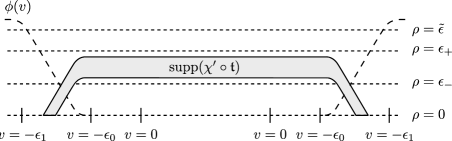
Figure 6. Setup for energy estimates near $\overline{C_{-}}$: The shaded region is the support of $\chi^{\prime}\circ\mathfrak{t}$, where $-\chi^{\prime}$ is used to dominate $\chi$ to give positivity in the energy estimate; near $\rho=0$ and on $\operatorname{supp}(\chi\circ\mathfrak{t})$, i.e. in the region between $\rho=0$ and the shaded region, a sufficiently large weight $\rho^{-\ell}$ gives positivity.

We have seen that the existence of appropriate timelike functions, such as $\mathfrak{t}$, in a neighborhood of $\overline{C_{+}}$ and $\overline{C_{-}}$ is automatic (in a slightly degenerate sense at $\overline{C_{\pm}}$ themselves) when $\frac{d\rho}{\rho}$ is timelike in these regions; indeed these functions could be extended to a neighborhood of $C_{0}$ if $v$ is appropriately chosen. In order to conclude that elements of $\operatorname{Ker}L$ and $\operatorname{Ker}L^{*}$ vanish globally, however, we need to control all of the interior of $M$. This can be accomplished by showing global hyperbolicity of $M^{\circ}$, which in turn can be seen by applying a result due to Geroch [16]. Namely, by [16, Theorem 11] it suffices to show that a suitable $\mathcal{S}$ is a Cauchy surface, which by [16, Property 6] follows if we show that $\mathcal{S}$ is achronal, closed, and every null-geodesic intersects and then re-emerges from $\mathcal{S}$. In order to define $\mathcal{S}$, it is useful to define $\widehat{\mathfrak{t}}=\psi\circ\mathfrak{t}$ in $U_{-}$, where $\psi\in C^{\infty}(\mathbb{R})$, $\psi^{\prime}\geq 0$, $\psi(t)=t$ near $t\leq\epsilon_{-}$, $\psi^{\prime}(t)>0$ for $t<\epsilon_{+}$, $\psi^{\prime}(t)=0$ for $t\geq\epsilon_{+}$; let $T=\psi(\epsilon_{+})>\epsilon_{-}$. Further, extend $\widehat{\mathfrak{t}}$ to $M$ as $=T$ outside $U_{-}$; since $U_{-}\cap\mathfrak{t}^{-1}((-\infty,\epsilon_{+}])$ is compact, this gives a $C^{\infty}$ function on $M$. Thus, $\widehat{\mathfrak{t}}\in C^{\infty}(M)$ is a globally weakly time-like function in that $\widehat{G}(d\widehat{\mathfrak{t}},d\widehat{\mathfrak{t}})\geq 0$, and it is strictly time-like in $M^{\circ}\cap\mathfrak{t}^{-1}((-\infty,\epsilon_{+}))$. In particular, it is monotone along all null-geodesics. Further, $\widehat{\mathfrak{t}}=0$ at $S_{-}$ and $\widehat{\mathfrak{t}}=T>0$ at $S_{+}$, indeed near $S_{+}$. Then we claim that $\mathcal{S}=\widehat{\mathfrak{t}}^{-1}(\epsilon_{-})\cap M^{\circ}$ is a Cauchy surface.

Now, $\mathcal{S}$ is closed in $M^{\circ}$ since $\overline{\mathcal{S}}$ is closed in $M$; indeed it is a closed embedded submanifold. By our non-trapping assumption, every null-geodesic in $M^{\circ}$ tends to $S_{+}$ in one direction and $S_{-}$ in the other direction, so on future oriented null-geodesics (ones tending to $S_{+}$), $\widehat{\mathfrak{t}}$ is monotone increasing, attaining all values in $(0,T]$. Since at the $\epsilon_{-}$ level set of $\mathfrak{t}$, hence of $\widehat{\mathfrak{t}}$, $d\widehat{\mathfrak{t}}$ is strictly time-like, the value $\epsilon_{-}$ is attained exactly once for $\widehat{\mathfrak{t}}$ along null-geodesics. Thus, every null-geodesic intersects $\mathcal{S}$ and then re-emerges from it. Finally, $\mathcal{S}$ is achronal, i.e. there exist no time-like curves connecting two points on $\mathcal{S}$: any future oriented time-like curve (meaning with tangent vector in the time-like cone whose boundary is the future light cone) in $M^{\circ}\cap\mathfrak{t}^{-1}((-\infty,\epsilon_{+}))$ has $\widehat{\mathfrak{t}}$ monotone increasing, with the increase being strict near $\mathcal{S}$, so again the value $\epsilon_{-}$ can be attained at most once on such a curve. In summary, this proves that $M^{\circ}$ is globally hyperbolic, so every solution of $Lu=0$ with vanishing Cauchy data on $\mathcal{S}$ vanishes identically, in particular by what we have observed, $\operatorname{Ker}L$ and $\operatorname{Ker}L^{*}$ are trivial on the indicated spaces.

In summary:

Theorem 5.3.

If $(M,g)$ is a non-trapping Lorentzian scattering metric in the sense of [2], $|l|<1$, and

1. The induced asymptotically hyperbolic resolvents $\mathcal{R}_{C_{\pm}}$ have no poles in $\operatorname{Im}\sigma\geq-|l|$,

2. $\frac{d\rho}{\rho}$ is timelike near $\overline{C_{+}}\cup\overline{C_{-}}$,

then for order functions $m\in C^{\infty}({}^{{\mathrm{b}}}S^{*}M)$ satisfying (LABEL:eq:m-decreasing) and (5.9), the forward problem for the conjugated wave operator $L$, i.e. with $L$ considered as a map

$$L:\mathcal{X}^{m,l}\to\mathcal{Y}^{m-1,l},$$

is invertible.

Extending the notation of [2], especially §4, we denote by $H_{{\mathrm{b}}}^{m,l,k}(M)$, where $m,l\in\mathbb{R},k\in\mathbb{N}_{0}$, the space of all $u\in H_{{\mathrm{b}}}^{m,l}(M)$ (i.e. $u\in\rho^{l}H^{m}_{\mathrm{b}}(M)$, where $\rho$ is the boundary defining function of $M$) such that $\mathcal{M}^{j}u\in H_{{\mathrm{b}}}^{m,l}(M)$ for all $0\leq j\leq k$. Here, $\mathcal{M}\subset\Psi_{\mathrm{b}}^{1}(M)$ is the $\Psi_{\mathrm{b}}^{0}(M)$-module of pseudodifferential operators with principal symbol vanishing on the radial set $\mathcal{R}_{+}$ of the operator $L=\rho^{-(n-2)/2}\rho^{-2}\Box_{g}\rho^{(n-2)/2}$; in the coordinates $\rho,v,y$ as in [2] ($\rho$ being as above, $v$ a defining function of the light cone at infinity within $\partial M$, $y$ coordinates within in the light cone at infinity), $\mathcal{M}$ has local generators $\rho\partial_{\rho},\rho\partial_{v},v\partial_{v},\partial_{y}$. Then the results of [2], concretely Proposition 4.4, extend our theorem to the spaces with module regularity.

Namely the reference, [2, Proposition 4.4], guarantees the module regularity $u\in H_{{\mathrm{b}}}^{m,l,k}(M)$ of a solution $u$ of $Lu=f$ if $f$ has matching module regularity $f\in H_{{\mathrm{b}}}^{m-1,l,k}(M)$ and if $u$ is in $H_{{\mathrm{b}}}^{m+k,l}(M)$ near $\overline{C_{-}}$. To be precise, this Proposition in [2] is stated making the stronger assumption, $f\in H_{{\mathrm{b}}}^{m-1+k,l}(M)$. However, the proof goes through for just $f\in H_{{\mathrm{b}}}^{m-1,l,k}(M)$ in a completely analogous manner to the result of Haber and Vasy [19, Theorem 6.3], where (in the boundaryless setting, for a Lagrangian radial set) the result is stated in this generality.

If $f\in H_{{\mathrm{b}}}^{m-1,l,k}(M)$, then in particular $f$ is locally in $H_{{\mathrm{b}}}^{m+k-1,l}$ near $\overline{C_{-}}$, thus, taking into account that $m+l>1/2$ already there, $u$ is in $H_{{\mathrm{b}}}^{m+k,l}$ in that region by Proposition 5.2 (by the first case there, i.e. in the high regularity regime). Thus, an application of the closed graph theorem gives the following boundedness result:

Theorem 5.4.

Under the assumptions of Theorem 5.3, $L^{-1}$ has the property that it restricts to

$$L^{-1}:H_{{\mathrm{b}}}^{m-1,l,k}\to H_{{\mathrm{b}}}^{m,l,k},\ k\geq 0,$$

as a bounded map.

In particular, letting $\Omega=\{\widetilde{\mathfrak{t}}\geq 0\}$, where $\widetilde{\mathfrak{t}}=\widehat{\mathfrak{t}}-\epsilon_{-}$ so that it attains the value $0$ within $M\setminus(\overline{C_{+}}\cup\overline{C_{-}})$, we have a forward solution operator $S$ of $L$ which maps $H_{{\mathrm{b}}}^{m-1,l,k}(\Omega)^{\bullet}$ into $H_{{\mathrm{b}}}^{m,l,k}(\Omega)^{\bullet}$, given that $m+l<1/2$; let us assume that $m$ is constant in $\Omega$. Here, $H_{{\mathrm{b}}}^{m,l,k}(\Omega)^{\bullet}$ consists of supported distributions at $\partial\Omega\cap C_{0}^{\circ}=\{\widetilde{\mathfrak{t}}=0\}$.

Remark 5.5.

Using the arguments leading to Theorem 5.3 in the current, forward problem, setting, but now also using standard energy estimates near the artificial boundary $\widetilde{\mathfrak{t}}=0$ of $\Omega$, we see that if suffices to control the resonances of the asymptotically hyperbolic resolvent in the upper cap $C_{+}$ in order to ensure the invertibility of the forward problem.

5.2. Algebra properties of $H_{{\mathrm{b}}}^{m,-\infty,k}$

In order to discuss non-linear wave equations on an asymptotically Minkowski space, we need to discuss the algebra properties of $H_{{\mathrm{b}}}^{m,-\infty,k}=\bigcup_{l\in\mathbb{R}}H_{{\mathrm{b}}}^{m,l,k}$. Even though we are only interested in the space $H_{{\mathrm{b}}}^{m,-\infty,k}(\Omega)^{\bullet}$, we consider $H_{{\mathrm{b}}}^{m,-\infty,k}(M)$, where $m$ is constant on $M$ for notational simplicity, and the results we prove below are valid for $H_{{\mathrm{b}}}^{m,-\infty,k}(\Omega)^{\bullet}$ by the same proofs.

We start with the following lemma:

Lemma 5.6.

Let $l_{1},l_{2}\in\mathbb{R}$, $k>n/2$. Then $H_{{\mathrm{b}}}^{0,l_{1},k}\cdot H_{{\mathrm{b}}}^{0,l_{2},k}\subset H_{{\mathrm{b}}}^{0,l_{1}+l_{2}-1/2,k}$.

Proof.

The generators $\rho\partial_{\rho},\rho\partial_{v},v\partial_{v},\partial_{y}$ of $\mathcal{M}$ take on a simpler form if we blow up the point $(\rho,v)=(0,0)$. It is most convenient to use projective coordinates on the blown-up space, namely:

1. Near the interior of the front face, we use the coordinates $\widetilde{\rho}=\rho\geq 0$ and $s=v/\rho\in\mathbb{R}$. We compute $\rho\partial_{\rho}=\widetilde{\rho}\partial_{\widetilde{\rho}}-s\partial_{s}$, $v\partial_{v}=s\partial_{s}$, $\rho\partial_{v}=\partial_{s}$; and since $\frac{d\rho}{\rho}\,dv\,dy=d\widetilde{\rho}\,ds\,dy$ (this is the b-density from $H_{{\mathrm{b}}}^{0,l,k}$), the space $H_{{\mathrm{b}}}^{0,l,k}$ becomes

   $$A^{l,k}:=\{u\in\widetilde{\rho}^{l}L^{2}(d\widetilde{\rho}\,ds\,dy)\colon\mathcal{A}^{j}u\in\widetilde{\rho}^{l}L^{2}(d\widetilde{\rho}\,ds\,dy),0\leq j\leq k\},$$

   where $\mathcal{A}$ is the $C^{\infty}$-module of differential operators generated by $\partial_{s},\widetilde{\rho}\partial_{\widetilde{\rho}},\partial_{y}$.

   Now, observe that $\widetilde{\rho}^{l}L^{2}(d\widetilde{\rho}\,ds\,dy)=\widetilde{\rho}^{l-1/2}L^{2}(\tfrac{d\widetilde{\rho}}{\rho}\,ds\,dy)$; therefore, we can rewrite

   $$A^{l,k} =\{u\in\widetilde{\rho}^{l-1/2}L^{2}(\tfrac{d\widetilde{\rho}}{\rho}\,ds\,dy)\colon\mathcal{A}^{j}u\in\widetilde{\rho}^{l-1/2}L^{2}(\tfrac{d\widetilde{\rho}}{\rho}\,ds\,dy),0\leq j\leq k\}$$

   $$=\widetilde{\rho}^{l-1/2}H_{{\mathrm{b}}}^{k}(\tfrac{d\widetilde{\rho}}{\rho}\,ds\,dy).$$

   In particular, by the Sobolev algebra property, Lemma 2.26, and the locality of the multiplication, choosing $k>n/2$ ensures that $\widetilde{\rho}^{l_{1}-1/2}H_{{\mathrm{b}}}^{k}\cdot\widetilde{\rho}^{l_{2}-1/2}H_{{\mathrm{b}}}^{k}\subset\widetilde{\rho}^{l_{1}+l_{2}-1}H_{{\mathrm{b}}}^{k}$, which is to say $A^{l_{1},k}\cdot A^{l_{2},k}\subset A^{l_{1}+l_{2}-1/2,k}$.

2. Near either corner of the blown-up space, we use $\widetilde{v}=v$ and $t=\rho/v$ (say, $\widetilde{v}\geq 0,t\geq 0$). We compute $\rho\partial_{\rho}=t\partial_{t}$, $v\partial_{v}=\widetilde{v}\partial_{\widetilde{v}}-t\partial_{t}$, $\rho\partial_{v}=t\widetilde{v}\partial_{\widetilde{v}}-t^{2}\partial_{t}$; and since $\frac{d\rho}{\rho}\,dv\,dy=\frac{dt}{t}\,d\widetilde{v}\,dy$, the space $H_{{\mathrm{b}}}^{0,l,k}$ becomes

   $$B^{l,k}:=\{u\in(t\widetilde{v})^{l}L^{2}(\tfrac{dt}{t}\,d\widetilde{v}\,dy)\colon\mathcal{B}^{j}u\in(t\widetilde{v})^{l}L^{2}(\tfrac{dt}{t}\,d\widetilde{v}\,dy),0\leq j\leq k\},$$

   where $\mathcal{B}$ is the $C^{\infty}$-module of differential operators generated by $t\partial t,\widetilde{v}\partial_{\widetilde{v}},\partial_{y}$. Again, we can rewrite this as

   $$B^{l,k}=t^{l}\widetilde{v}^{l-1/2}H_{{\mathrm{b}}}^{k}(\tfrac{dt}{t}\,\tfrac{d\widetilde{v}}{\widetilde{v}}\,dy),$$

   which implies that for $k>n/2$,

   $$B^{l_{1},k}\cdot B^{l_{2},k}\subset t^{l_{1}+l_{2}}v^{l_{1}+l_{2}-1}H_{{\mathrm{b}}}^{k}(\tfrac{dt}{t}\,\tfrac{d\widetilde{v}}{\widetilde{v}}\,dy)\subset B^{l_{1}+l_{2}-1/2,k}.$$

To relate these two statements to the statement of the lemma, we use cutoff functions $\chi_{A},\chi_{B}$ to localize within the two coordinate systems. More precisely, choose a cutoff function $\chi\in C^{\infty}_{c}(\mathbb{R}_{s})$ such that $\chi(s)\equiv 1$ near $s=0$, $\chi(s)=0$ for $|s|\geq 2$, and $\chi^{1/2}\in C^{\infty}_{c}(\mathbb{R}_{s})$. Then multiplication with $\chi_{A}(\rho,v):=\chi(v/\rho)$ is a continuous map $H_{{\mathrm{b}}}^{0,l,k}\to A^{l,k}$. Indeed, to check this, one simply observes that $\mathcal{M}^{j}\chi_{A}\in L^{\infty}$ for all $j\in\mathbb{N}_{0}$. Similarly, letting $\chi_{B}(\rho,v):=1-\chi_{A}(\rho,v)$, multiplication with $\chi_{B}$ is a continuous map $H_{{\mathrm{b}}}^{0,l,k}\to B^{l,k}$. Finally, note that we have $A^{l,k},B^{l,k}\subset H_{{\mathrm{b}}}^{0,l,k}$.

To put everything together, take $u_{j}\in H_{{\mathrm{b}}}^{0,l_{j},k}$ ($j=1,2$), then

$$u_{1}u_{2}=(\chi_{A}u_{1})(\chi_{A}u_{2})+(\chi_{B}u_{1})(\chi_{B}u_{2})+(\chi_{A}u_{1})(\chi_{B}u_{2})+(\chi_{B}u_{1})(\chi_{A}u_{2}).$$

The first two terms then lie in $H_{{\mathrm{b}}}^{0,l_{1}+l_{2}-1/2,k}$. To deal with the third term, write

$$(\chi_{A}u_{1})(\chi_{B}u_{2})=(\chi_{A}^{1/2}u_{1})(\chi_{A}^{1/2}\chi_{B}u_{2})\in A^{l_{1},k}\cdot A^{l_{2},k}\subset H_{{\mathrm{b}}}^{0,l_{1}+l_{2}-1/2,k};$$

likewise for the fourth term. Thus, $u_{1}u_{2}\in H_{{\mathrm{b}}}^{0,l_{1}+l_{2}-1/2,k}$, as claimed. ∎

Remark 5.7.

The proof actually shows more, namely that

$$H_{{\mathrm{b}}}^{0,l,k}H_{{\mathrm{b}}}^{0,l^{\prime},k}\subset\rho_{\textnormal{ff}}^{-1/2}H_{{\mathrm{b}}}^{0,l+l^{\prime},k},$$ (5.10)

where $\rho_{\textnormal{ff}}$ is the defining function of the front face $\rho=v=0$, e.g. $\rho_{\textnormal{ff}}=(\rho^{2}+v^{2})^{1/2}$. The reason for (5.10) to be a natural statement is that module- and b-derivatives are the same away from $\rho=v=0$, hence regularity with respect to the module $\mathcal{M}$ is, up to a weight, which is a power of $\rho_{\textnormal{ff}}$, the same as b-regularity.

More abstractly speaking, the above proof shows the following: If $\rho_{b}$ denotes a boundary defining function of the other boundary hypersurface of $[M;S_{+}]$, i.e. $\partial[M;S_{+}]\setminus\textnormal{ff}$, then

$$H_{{\mathrm{b}}}^{0,l,k}\cong\rho_{\textnormal{ff}}^{-1/2}(\rho_{\textnormal{ff}}\rho_{b})^{l}H_{{\mathrm{b}}}^{k}([M;S_{+}]).$$

Note that one can also show this in one step, introducing the coordinates $\rho_{\textnormal{ff}}\geq 0$ and $s=v/(\rho+\rho_{\textnormal{ff}})\in[-1,1]$ on $[M;S_{+}]$ in a neighborhood of ff, and mimicking the above proof, which however is computationally less convenient.

Remark 5.8.

We can extend the lemma to $H_{{\mathrm{b}}}^{m,l,k}H_{{\mathrm{b}}}^{m,l^{\prime},k}\subset H_{{\mathrm{b}}}^{m,l+l^{\prime}-1/2,k}$ for $m\in\mathbb{N}_{0}$ using the Leibniz rule to distribute the $m$ b-derivatives among the two factors, and then using the lemma for the case $m=0$.

The following corollary, which will play an important role in §5.5, improves Lemma 5.6 if we have higher b-regularity.

Corollary 5.9.

Let $k>n/2$, $0\leq\delta<1/n$ and $l,l^{\prime}\in\mathbb{R}$. Then

1. $H_{{\mathrm{b}}}^{1,l,k}H_{{\mathrm{b}}}^{0,l^{\prime},k}\subset H_{{\mathrm{b}}}^{0,l+l^{\prime}-1/2+\delta,k}$.

2. $H_{{\mathrm{b}}}^{1,l,k}H_{{\mathrm{b}}}^{1,l^{\prime},k}\subset H_{{\mathrm{b}}}^{1,l+l^{\prime}-1/2+\delta,k}$.

Proof.

Take $s=1/(2\delta)>n/2$, then

$$H_{{\mathrm{b}}}^{s,l,k}H_{{\mathrm{b}}}^{0,l^{\prime},k}\subset H_{{\mathrm{b}}}^{0,l+l^{\prime},k};$$ (5.11)

indeed, using the Leibniz rule to distribute the $k$ module derivatives among the two factors and cancelling the weights, this amounts to showing that $H_{{\mathrm{b}}}^{s,0,k_{1}}H_{{\mathrm{b}}}^{0,0,k_{2}}\subset H_{{\mathrm{b}}}^{0,0,0}$ for $k_{1}+k_{2}\geq k$; but this is true even for $k_{1}=k_{2}=0$, since $H_{{\mathrm{b}}}^{s}$ is a multiplier on $H_{{\mathrm{b}}}^{0}$ provided $s>n/2$.

The lemma on the other hand gives

$$H_{{\mathrm{b}}}^{0,l,k}H_{{\mathrm{b}}}^{0,l^{\prime},k}\subset\rho^{-1/2}H_{{\mathrm{b}}}^{0,l+l^{\prime},k}.$$ (5.12)

Interpolating in the first factor between (5.11) and (5.12) thus gives the first statement.

For the second statement, use the Leibniz rule to distribute the one b-derivative to either factor; then, one has to show $H_{{\mathrm{b}}}^{1,l,k}H_{{\mathrm{b}}}^{0,l^{\prime},k}\subset H_{{\mathrm{b}}}^{0,l+l^{\prime}-1/2+\delta,k}$, and the same inclusion with $l$ and $l^{\prime}$ switched, which is what we just proved. ∎

Lemma 5.6 and the remark following it imply that for $u\in H_{{\mathrm{b}}}^{m,l,k}$, $p\geq 1$, with $m\geq 0,k>n/2$, we have $u^{p}\in H_{{\mathrm{b}}}^{m,pl-(p-1)/2,k}$; in fact, $u^{p}\in\rho_{\textnormal{ff}}^{-(p-1)/2}H_{{\mathrm{b}}}^{m,pl,k}$, see Remark 5.7. Using Corollary 5.9, we can improve this to the statement $u\in H_{{\mathrm{b}}}^{m,l,k}$ $\Rightarrow$ $u^{p}\in H_{{\mathrm{b}}}^{m,pl-(p-1)/2+(p-1)\delta,k}$ for $m\geq 1$.

For non-linearities that only involve powers $u^{p}$, we can afford to lose differentiability, as at the end of §4.2, and gain decay in return, as the following lemma shows.

Lemma 5.10.

Let $\alpha>1/2$, $l\in\mathbb{R}$, $k\in\mathbb{N}_{0}$. Then $\rho_{\textnormal{ff}}^{-\alpha}H_{{\mathrm{b}}}^{0,l,k}\subset\rho^{1/2-\alpha}H_{{\mathrm{b}}}^{-1,l,k}$, where $\rho_{\textnormal{ff}}=(\rho^{2}+v^{2})^{1/2}$.

Proof.

We may assume $l=0$, and that $u$ is supported in $|v|<1$, $\rho<1$. First, consider the case $k=0$. Let $u\in\rho_{\textnormal{ff}}^{-\alpha}H_{{\mathrm{b}}}^{0}$, and put

$$\widetilde{u}(\rho,v,y)=\int_{-\infty}^{v}u(\rho,w,y)\,dw,$$

so $\partial_{v}\widetilde{u}=u$. We have to prove $\chi\widetilde{u}\in\rho^{1/2-\alpha}H_{{\mathrm{b}}}^{0}$ if $\chi\equiv 1$ near $\operatorname{supp}u$, which implies $u\in H_{{\mathrm{b}}}^{-1}$, as $\partial_{v}:H_{{\mathrm{b}}}^{0}\to H_{{\mathrm{b}}}^{-1}$, and the b-Sobolev space are local spaces. But

$$|\widetilde{u}(\rho,v,y)|^{2}\leq\left(\int_{-1}^{1}\rho_{\textnormal{ff}}(\rho,w)^{2\alpha}|u(\rho,w,y)|^{2}\,dw\right)\int_{-1}^{1}\rho_{\textnormal{ff}}(\rho,w)^{-2\alpha}\,dw;$$ (5.13)

now,

$$\int_{-1}^{1}\rho_{\textnormal{ff}}^{-2\alpha}\,dw=\rho^{1-2\alpha}\int_{-1/\rho}^{1/\rho}\frac{dz}{(1+|z|^{2})^{\alpha}}\lesssim\rho^{1-2\alpha}$$

for $\alpha>1/2$, therefore, with the $v$ integral considered on a fixed interval, say $|v|<2$ (notice that the right hand side in (5.13) is independent of $v$!),

$$\iiint\rho^{2\alpha-1}|\widetilde{u}(\rho,v,y)|^{2}\,\frac{d\rho}{\rho}\,dv\,dy\lesssim\iiint\rho_{\textnormal{ff}}^{2\alpha}|u(\rho,w,y)|^{2}\,\frac{d\rho}{\rho}\,dw\,dy,$$

proving the claim for $k=0$. Now, $\rho\partial_{\rho}$ and $\partial_{y}$ just commute with this calculation, so the corresponding derivatives are certainly well-behaved. On the other hand, $\partial_{v}\widetilde{u}=u$, so the estimates involving at least one $v$-derivative are just those for $u$ itself. ∎

Corollary 5.11.

Let $k,p\in\mathbb{N}$ be such that $k>n/2$, $p\geq 2$. Let $l\in\mathbb{R}$, $u\in H_{{\mathrm{b}}}^{0,l,k}$. Then $u^{p}\in H_{{\mathrm{b}}}^{-1,lp-(p-1)/2+1/2-\delta,k}$ with $\delta=0$ if $p\geq 3$ and $\delta>0$ if $p=2$.

Proof.

This follows from $u^{p}\in\rho_{\textnormal{ff}}^{-(p-1)/2-\delta}H_{{\mathrm{b}}}^{0,lp,k}$ and the previous lemma, using that $(p-1)/2+\delta>1/2$ with $\delta$ as stated. ∎

In other words, we gain the decay $\rho^{1/2-\delta}$ if we give up one derivative.

5.3. A class of semilinear equations

We are now set to discuss solutions to non-linear wave equations on an asymptotically Minkowski space. Under the assumptions of Theorem 5.3, we obtain a forward solution operator $S\colon H_{{\mathrm{b}}}^{m-1,l,k}(\Omega)^{\bullet}\to H_{{\mathrm{b}}}^{m,l,k}(\Omega)^{\bullet}$ of $P=\rho^{-(n-2)/2}\rho^{-2}\Box_{g}\rho^{(n-2)/2}$ provided $|l|<1,m+l<1/2$ and $k\geq 0$.

Undoing the conjugation, we obtain a forward solution operator

$$\widetilde{S} =\rho^{(n-2)/2}S\rho^{-2}\rho^{-(n-2)/2},$$

$$\widetilde{S} \colon H_{{\mathrm{b}}}^{m-1,l+(n-2)/2+2,k}(\Omega)^{\bullet}\to H_{{\mathrm{b}}}^{m,l+(n-2)/2,k}(\Omega)^{\bullet}$$

of $\Box_{g}$.

Since $g$ is a Lorentzian scattering metric, the natural vector fields to appear in a non-linear equation are scattering vector fields; more generally, since the analysis is carried out on b-spaces, we indeed allow b-vector fields in the following statement:

Theorem 5.12.

Let

$$q\colon H_{{\mathrm{b}}}^{m,l+(n-2)/2,k}(\Omega)^{\bullet}\times H_{{\mathrm{b}}}^{m-1,l+(n-2)/2,k}(\Omega;{}^{{\mathrm{b}}}T^{*}\Omega)^{\bullet}\to H_{{\mathrm{b}}}^{m-1,l+(n-2)/2+2,k}(\Omega)^{\bullet}$$

be a continuous function with $q(0,0)=0$ such that there exists a continuous non-decreasing function $L\colon\mathbb{R}_{\geq 0}\to\mathbb{R}$ satisfying

$$\|q(u,{}^{{\mathrm{b}}}du)-q(v,{}^{{\mathrm{b}}}dv)\|\leq L(R)\|u-v\|,\quad\|u\|,\|v\|\leq R.$$

Then there is a constant $C_{L}>0$ so that the following holds: If $L(0)<C_{L}$, then for small $R>0$, there exists $C>0$ such that for all $f\in H_{{\mathrm{b}}}^{m-1,l+(n-2)/2+2,k}(\Omega)^{\bullet}$ with norm $\leq C$, the equation

$$\Box_{g}u=f+q(u,{}^{{\mathrm{b}}}du)$$

has a unique solution $u\in H_{{\mathrm{b}}}^{m,l+(n-2)/2,k}(\Omega)^{\bullet}$, with norm $\leq R$, that depends continuously on $f$.

Proof.

Use the Banach fixed point theorem as in the proof of Theorem 2.25. ∎

Remark 5.13.

Here, just as in Theorem 4.10, we can also allow $q$ to depend on $\Box_{g}u$ as well.

5.4. Semilinear equations with polynomial non-linearity

Next, we want to find a forward solution of the semilinear PDE

$$\Box_{g}u=f+cu^{p}X(u),$$

where $c\in C^{\infty}(M)$, $p\in\mathbb{N}_{0}$, and $X(u)=\prod_{j=1}^{q}\rho V_{j}(u)$ is a $q$-fold product of derivatives of $u$ along scattering vector fields; here, $V_{j}$ are b-vector fields. Let us assume $p+q\geq 2$ in order for the equation to be genuinely non-linear. We rewrite the PDE as

$$L(\rho^{-(n-2)/2}u) =\rho^{-(n-2)/2-2}f+c\rho^{-2}\rho^{(p-1)(n-2)/2}(\rho^{-(n-2)/2}u)^{p}$$

$$\qquad\times\prod_{j=1}^{q}\rho V_{j}(\rho^{(n-2)/2}\rho^{-(n-2)/2}u).$$

Introducing $\widetilde{u}=\rho^{-(n-2)/2}u$ and $\widetilde{f}=\rho^{-(n-2)/2-2}f$ yields the equation

$$L\widetilde{u} =\widetilde{f}+c\rho^{(p-1)(n-2)/2-2}\widetilde{u}^{p}\prod_{j=1}^{q}\rho^{n/2}(f_{j}\widetilde{u}+V_{j}\widetilde{u})$$

$$=\widetilde{f}+c\rho^{(p-1)(n-2)/2+qn/2-2}\widetilde{u}^{p}\prod_{j=1}^{q}(f_{j}\widetilde{u}+V_{j}\widetilde{u}),$$ (5.14)

where the $f_{j}$ are smooth functions. Now suppose that $\widetilde{u}\in H_{{\mathrm{b}}}^{m,l,k}(\Omega)^{\bullet}$ with $m+l<1/2,m\geq 1,k>n/2$ (so that $H_{{\mathrm{b}}}^{m-1,-\infty,k}(\Omega)^{\bullet}$ is an algebra), then the second summand of the right hand side of (5.14) lies in $H_{{\mathrm{b}}}^{m-1,\ell,k}(\Omega)^{\bullet}$, where

$$\ell=(p-1)(n-2)/2+qn/2-2+pl-(p-1)/2+ql-(q-1)/2-1/2.$$

For this space to lie in $H_{{\mathrm{b}}}^{m-1,l,k}(\Omega)^{\bullet}$ (which we want in order to be able to apply the solution operator $S$ and land in $H_{{\mathrm{b}}}^{m,l,k}(\Omega)^{\bullet}$ so that a fixed point argument as in §2 can be applied), we thus need $\ell\geq l$, which can be rewritten as

$$(p-1)(l+(n-3)/2)+q(l+(n-1)/2)\geq 2.$$ (5.15)

For $m=1$ and $l<1/2-m$ less than, but close to $-1/2$, we thus get the condition

$$(p-1)(n-4)+q(n-2)>4.$$

If there are only non-linearities involving derivatives of $u$, i.e. $p=0$, we get the condition $q>1+2/(n-2)$, i.e. quadratic non-linearities are fine for $n\geq 5$, cubic ones for $n\geq 4$.

Note that if $q=0$, we can actually choose $m=0$ and $l<1/2$ close to $1/2$, and we have Corollary 5.11 at hand. Thus we can improve (5.15) to $(p-1)(1/2+(n-3)/2)>2-1/2$, i.e. $p>1+3/(n-2)$, hence quadratic non-linearities can be dealt with if $n\geq 6$, whereas cubic non-linearities are fine as long as $n\geq 4$. Observe that this condition on $p$ always implies $p>1$, which is a natural condition, since $p=1$ would amount to changing $\Box_{g}$ into $\Box_{g}-m^{2}$ (if one chooses the sign appropriately). But the Klein-Gordon operator naturally fits into a scattering framework, as mentioned in the Introduction, i.e. requires a different analysis; we will not pursue this further in this paper.

To summarize the general case, note that $\widetilde{u}\in H_{{\mathrm{b}}}^{m,l,k}(\Omega)^{\bullet}$ is equivalent to $u\in H_{{\mathrm{b}}}^{m,l+(n-2)/2,k}(\Omega)^{\bullet}$, and $\widetilde{f}\in H_{{\mathrm{b}}}^{m-1,l,k}(\Omega)^{\bullet}$ to $f\in H_{{\mathrm{b}}}^{m-1,l+(n-2)/2+2,k}(\Omega)^{\bullet}$; thus:

Theorem 5.14.

Let $|l|<1,m+l<1/2,k>n/2$, and assume that $p,q\in\mathbb{N}_{0}$, $p+q\geq 2$, satisfy condition (5.15) or the weaker conditions given above in the cases where $p=0$ or $q=0$; let $m\geq 0$ if $q=0$, otherwise let $m\geq 1$. Moreover, let $c\in C^{\infty}(M)$ and $X(u)=\prod_{j=1}^{q}X_{j}u$, where $X_{j}$ is a scattering vector field on $M$. Then for small enough $R>0$, there exists a constant $C>0$ such that for all $f\in H_{{\mathrm{b}}}^{m-1,l+(n-2)/2+2,k}(\Omega)^{\bullet}$ with norm $\leq C$, the equation

$$\Box_{g}u=f+cu^{p}X(u)$$

has a unique solution $u\in H_{{\mathrm{b}}}^{m,l+(n-2)/2,k}(\Omega)^{\bullet}$, with norm $\leq R$, that depends continuously on $f$.

The same conclusion holds if the non-linearity is a finite sum of terms of the form $cu^{p}X(u)$, provided each such term separately satisfies (5.15).

Proof.

Reformulating the PDE in terms of $\widetilde{u}$ and $\widetilde{f}$ as above, this follows from an application of the Banach fixed point theorem to the map

$$H_{{\mathrm{b}}}^{m,l,k}(\Omega)^{\bullet}\ni\widetilde{u}\mapsto S\biggl{(}\widetilde{f}+c\rho^{(p-1)(n-2)/2+qn/2-2}\widetilde{u}^{p}\prod_{j=1}^{q}(f_{j}\widetilde{u}+V_{j}\widetilde{u})\biggr{)}\in H_{{\mathrm{b}}}^{m,l,k}(\Omega)^{\bullet}$$

with $m,l,k$ as in the statement of the theorem. Here, $p+q\geq 2$ and the smallness of $R$ ensure that this map is a contraction on the ball of radius $R$ in $H_{{\mathrm{b}}}^{m,l,k}(\Omega)^{\bullet}$. ∎

Remark 5.15.

If the derivatives in the non-linearity only involve module derivatives, we get a slightly better result since we can work with $\widetilde{u}\in H_{{\mathrm{b}}}^{0,l,k}(\Omega)^{\bullet}$: Indeed, a module derivative falling on $\widetilde{u}$ gives an element of $H_{{\mathrm{b}}}^{0,l,k-1}(\Omega)^{\bullet}$, applied to which the forward solution operator produces an element of $H_{{\mathrm{b}}}^{1,l,k-1}(\Omega)^{\bullet}\subset H_{{\mathrm{b}}}^{0,l,k}(\Omega)^{\bullet}$.

The numerology works out as follows: In condition (5.15), we now take $l<1/2$ close to $1/2$, thus obtaining

$$(p-1)(n-2)+qn>4.$$

Thus, in the case that there are only derivatives in the non-linearity, i.e. $p=0$, we get $q>1+2/n$, which allows for quadratic non-linearities provided $n\geq 3$.

Remark 5.16.

Observe that we can improve (5.15) in the case $p\geq 1$, $q\geq 1$, $m\geq 1$ by using the $\delta$-improvement from Corollary 5.9, namely, the right hand side of (5.14) actually lies in $H_{{\mathrm{b}}}^{m-1,\ell,k}(\Omega)^{\bullet}$, where now

$$\ell=(p-1)(n-2)/2+qn/2-2+pl-(p-1)/2+(p-1)\delta+ql-(q-1)/2-1/2+\delta,$$

which satisfies $\ell\geq l$ if

$$(p-1)(l+(n-3)/2+\delta)+q(l+(n-1)/2)+\delta\geq 2,$$

which for $l<-1/2$ close to $-1/2$ means: $(p-1)(n-4+2\delta)+q(n-2)+2\delta>4$, where $0<\delta<1/n$.

Remark 5.17.

Let us compare the above result with Christodoulou’s [7]. A special case of his theorem states that the Cauchy problem for the wave equation on Minkowski space with small initial data in $H_{k,k-1}(\mathbb{R}^{n-1})$ admits a global solution $u\in H^{k}_{\mathrm{loc}}(\mathbb{R}^{n})$ with decay $|u(x)|\lesssim(1+(v/\rho)^{2})^{-(n-2)/2}$; here, $k=n/2+2$, and $n$ is assumed to $\geq 4$ and even; in case $n=4$, the non-linearity is moreover assumed to satisfy the null condition. The only polynomial non-linearity that we cannot deal with using the above argument is thus the null-form non-linearity in $4$ dimensions.

To make a further comparison possible, we express $H_{k,\delta}(\mathbb{R}^{n-1})$ as a b-Sobolev space on the radial compactification of $\mathbb{R}^{n-1}$: Note that $u\in H_{k,\delta}(\mathbb{R}^{n-1})$ is equivalent to $(\langle x\rangle D_{x})^{\alpha}u\in\langle x\rangle^{-\delta}L^{2}(\mathbb{R}^{n-1})$, $|\alpha|\leq k$. In terms of the boundary defining function $\rho$ of $\partial\overline{\mathbb{R}^{n-1}}$ and the standard measure $d\omega$ on the unit sphere $\mathbb{S}^{n-2}\subset\mathbb{R}^{n-1}$, we have $L^{2}(\mathbb{R}^{n-1})=L^{2}(\tfrac{d\rho}{\rho^{2}}\,\tfrac{dy}{\rho^{n-2}})=\rho^{(n-1)/2}L^{2}(\tfrac{d\rho}{\rho}\,dy)$, and thus $H_{k,\delta}(\mathbb{R}^{n-1})=\rho^{(n-1)/2+\delta}H^{k}_{\mathrm{b}}(\widetilde{\mathfrak{t}}=0)$. Therefore, converting the Cauchy problem into a forward problem, the forcing lies in $H_{{\mathrm{b}}}^{k,(n-1)/2+k-1,0}(\Omega)^{\bullet}=H_{{\mathrm{b}}}^{n/2+2,n+1/2,0}(\Omega)^{\bullet}$. Comparing this with the space $H^{0,l+(n-2)/2+2,n/2+1}_{\mathrm{b}}$ (with $l<1/2$) needed for our argument, we see that Christodoulou’s result applies to a regime of fast decay which is disjoint from our slow decay (or even mild growth) regime.

Remark 5.18.

In the case of non-linearities $u^{p}$, the result of Christodoulou [7] implies the existence of global solutions to $\Box_{g}u=f+u^{p}$ if the spacetime dimension $n$ is even and $n\geq 4$ if $p\geq 3$; in even dimensions $n\geq 6$, $p\geq 2$ suffices; the above result extends this to all dimensions satisfying the respective inequalities. In a somewhat similar context, see the work of Chruściel and Łȩski [9], it has been proved that $p\geq 2$ in fact works in all dimensions $n\geq 5$.

5.5. Semilinear equations with null condition

With $g$ the Lorentzian scattering metric on an asymptotically Minkowski space satisfying the assumptions of Theorem 5.3 as before, define the null form $Q({}^{{\mathrm{sc}}}du,{}^{{\mathrm{sc}}}dv)=g^{jk}\partial_{j}u\partial_{k}v$, and write $Q({}^{{\mathrm{sc}}}du)$ for $Q({}^{{\mathrm{sc}}}du,{}^{{\mathrm{sc}}}du)$. We are interested in solving the PDE

$$\Box_{g}u=Q({}^{{\mathrm{sc}}}du)+f.$$

The previous discussion solves this for $n\geq 5$; thus, let us from now on assume $n=4$. To make the computations more transparent, we will keep the $n$ in the notation and only substitute $n=4$ when needed. Rewriting the PDE in terms of the operator $L=\rho^{-2}\rho^{-(n-2)/2}\Box_{g}\rho^{(n-2)/2}$ as above, we get

$$L\widetilde{u}=\widetilde{f}+\rho^{-(n-2)/2-2}Q({}^{{\mathrm{sc}}}d(\rho^{(n-2)/2}\widetilde{u})),$$

where $\widetilde{u}=\rho^{-(n-2)/2}u$ and $\widetilde{f}=\rho^{-(n-2)/2-2}f$. We can write $Q({}^{{\mathrm{sc}}}du)=\tfrac{1}{2}\Box_{g}(u^{2})-u\Box_{g}u$, thus the PDE becomes

$$L\widetilde{u} =\widetilde{f}+\rho^{-(n-2)/2-2}\bigl{(}\tfrac{1}{2}\Box_{g}(\rho^{n-2}\widetilde{u}^{2})-\rho^{(n-2)/2}\widetilde{u}\Box_{g}(\rho^{(n-2)/2}\widetilde{u})\bigr{)}$$

$$=\widetilde{f}+\tfrac{1}{2}L(\rho^{(n-2)/2}\widetilde{u}^{2})-\rho^{(n-2)/2}\widetilde{u}L\widetilde{u}.$$

Since the results of §5.2 give small improvements on the decay of products of $H_{{\mathrm{b}}}^{1,*,*}$ functions with $H_{{\mathrm{b}}}^{m,*,*}$ functions ($m\geq 0$), one wants to solve this PDE on a function space that keeps track of these small improvements.

Definition 5.19.

For $l\in\mathbb{R},k\in\mathbb{N}_{0}$ and $\alpha\geq 0$, define the space $\mathcal{X}^{l,k,\alpha}:=\{v\in H_{{\mathrm{b}}}^{1,l+\alpha,k}(\Omega)^{\bullet}\colon Lv\in H_{{\mathrm{b}}}^{0,l,k}(\Omega)^{\bullet}\}$ with norm

$$\|v\|_{\mathcal{X}^{l,k,\alpha}}=\|v\|_{H_{{\mathrm{b}}}^{1,l+\alpha,k}(\Omega)^{\bullet}}+\|Lv\|_{H_{{\mathrm{b}}}^{0,l,k}(\Omega)^{\bullet}}.$$ (5.16)

By an argument similar to the one used in the proof of Theorem 2.25, we see that $\mathcal{X}^{l,k,\alpha}$ is a Banach space.

On $\mathcal{X}^{l,k,\alpha}$, which $\alpha>0$ chosen below, we want to run an iteration argument: Start by defining the operator $T\colon\mathcal{X}^{l,k,\alpha}\to H_{{\mathrm{b}}}^{1,-\infty,k}(\Omega)^{\bullet}$ by

$$T\colon\widetilde{u}\mapsto S\bigl{(}\widetilde{f}-\rho^{(n-2)/2}\widetilde{u}L\widetilde{u}\bigr{)}+\tfrac{1}{2}\rho^{(n-2)/2}\widetilde{u}^{2}.$$

Note that $\widetilde{u}\in\mathcal{X}^{l,k,\alpha}$ implies, using Corollary 5.9 with $\delta<1/n$,

$$\rho^{(n-2)/2}\widetilde{u}^{2} \in\rho^{(n-2)/2}H_{{\mathrm{b}}}^{1,2(l+\alpha)-1/2+\delta,k}(\Omega)^{\bullet}=H_{{\mathrm{b}}}^{1,2l+\alpha+(n-3)/2+\delta+\alpha,k}(\Omega)^{\bullet},$$

$$\rho^{(n-2)/2}\widetilde{u}L\widetilde{u} \in H_{{\mathrm{b}}}^{0,2l+\alpha+(n-3)/2+\delta,k}(\Omega)^{\bullet},$$ (5.17)

$$S(\rho^{(n-2)/2}\widetilde{u}L\widetilde{u}) \in H_{{\mathrm{b}}}^{1,2l+\alpha+(n-3)/2+\delta,k}(\Omega)^{\bullet},$$

where in the last inclusion, we need to require $1+(2l+\alpha+(n-3)/2+\delta)<1/2$, which for $n=4$ means

$$l<-1/2-(\alpha+\delta)/2;$$ (5.18)

let us assume from now on that this condition holds. Furthermore, (5.17) implies $T\widetilde{u}\in H_{{\mathrm{b}}}^{1,2l+\alpha+(n-3)/2+\delta,k}(\Omega)^{\bullet}$. Finally, we analyze

$$L(T\widetilde{u})\in H_{{\mathrm{b}}}^{0,2l+\alpha+(n-3)/2+\delta,k}(\Omega)^{\bullet}+\frac{1}{2}L(\rho^{(n-2)/2}\widetilde{u}^{2}).$$

Using that $L$ is a second-order b-differential operator, we have

$$\rho^{(n-2)/2} L(\widetilde{u}^{2})\in 2\rho^{(n-2)/2}\widetilde{u}L\widetilde{u}+\rho^{(n-2)/2}H_{{\mathrm{b}}}^{0,l+\alpha,k}(\Omega)^{\bullet}H_{{\mathrm{b}}}^{0,l+\alpha,k}(\Omega)^{\bullet}$$

$$\subset H_{{\mathrm{b}}}^{0,2l+\alpha+(n-3)/2+\delta,k}(\Omega)^{\bullet}+H_{{\mathrm{b}}}^{0,2(l+\alpha)+(n-3)/2,k}(\Omega)^{\bullet}$$

$$=H_{{\mathrm{b}}}^{0,2l+\alpha+(n-3)/2+\min\{\alpha,\delta\},k}(\Omega)^{\bullet},$$

which gives

$$L( \rho^{(n-2)/2}\widetilde{u}^{2})\in L(\rho^{(n-2)/2})\widetilde{u}^{2}+\rho^{(n-2)/2}L(\widetilde{u}^{2})$$

$$\hskip 77.49976pt+\rho^{(n-2)/2}H_{{\mathrm{b}}}^{1,l+\alpha,k}(\Omega)^{\bullet}H_{{\mathrm{b}}}^{0,l+\alpha,k}(\Omega)^{\bullet}$$

$$\subset H_{{\mathrm{b}}}^{1,2l+\alpha+(n-3)/2+\delta+\alpha,k}(\Omega)^{\bullet}+H_{{\mathrm{b}}}^{0,2l+\alpha+(n-3)/2+\min\{\alpha,\delta\},k}(\Omega)^{\bullet}$$

$$\hskip 51.6665pt+H_{{\mathrm{b}}}^{0,2l+\alpha+(n-3)/2+\delta+\alpha}(\Omega)^{\bullet}$$

$$=H_{{\mathrm{b}}}^{0,2l+\alpha+(n-3)/2+\min\{\alpha,\delta\},k}(\Omega)^{\bullet}.$$

Hence, putting everything together,

$$L(T\widetilde{u})\in H_{{\mathrm{b}}}^{0,2l+\alpha+(n-3)/2+\min\{\alpha,\delta\},k}(\Omega)^{\bullet}.$$

Therefore, we have $T\widetilde{u}\in\mathcal{X}^{l,k,\alpha}$ provided

$$2l +\alpha+(n-3)/2+\delta\geq l+\alpha$$

$$2l +\alpha+(n-3)/2+\min\{\alpha,\delta\}\geq l,$$

which for $0<\alpha<\delta$ and $n=4$ is equivalent to

$$l\geq-1/2-\delta,l\geq-1/2-2\alpha.$$ (5.19)

This is consistent with condition (5.18) if $-1/2-(\alpha+\delta)/2>-1/2-2\alpha$, i.e. if $\alpha>\delta/3$.

Finally, for the map $T$ to be well-defined, we need $S\widetilde{f}\in\mathcal{X}^{l,k,\alpha}$, hence $\widetilde{f}\in\operatorname{Ran}_{\mathcal{X}^{l,k,\alpha}}L$, which is in particular satisfied if $\widetilde{f}\in H_{{\mathrm{b}}}^{0,l+\alpha,k}(\Omega)^{\bullet}$. Indeed, since $1+l+\alpha<1-1/2-(\delta-\alpha)/2<1/2$ by condition (5.18), the element $S\widetilde{f}\in H_{{\mathrm{b}}}^{1,l+\alpha,k}(\Omega)^{\bullet}$ is well-defined.

We have proved:

Theorem 5.20.

Let $c\in\mathbb{C}$, $0<\delta<1/4$, $\delta/3<\alpha<\delta$, and let $-1/2-2\alpha\leq l<-1/2-(\alpha+\delta)/2$. Then for small enough $R>0$, there exists a constant $C>0$ such that for all $f\in H_{{\mathrm{b}}}^{0,l+3+\alpha,k}(\Omega)^{\bullet}$ with norm $\leq C$, the equation

$$\Box_{g}u=f+cQ({}^{{\mathrm{sc}}}du)$$

has a unique solution $u\in\mathcal{X}^{l+1,k,\alpha}$, with norm $\leq R$, that depends continuously on $f$.

References

- [1] Dean Baskin. A Strichartz estimate for de Sitter space. Annales Henri Poincare, arXiv:0909.2696, 14:221–252, 2013.
- [2] Dean Baskin, András Vasy, and Jared Wunsch. Asymptotics of radiation fields in asymptotically Minkowski space. Am. J. Math., to appear; arXiv:1212.5141.
- [3] Dean Baskin. A parametrix for the fundamental solution of the Klein-Gordon equation on asymptotically de Sitter spaces. J. Funct. Anal., 259(7):1673–1719, 2010.
- [4] Lydia Bieri. Part I: Solutions of the Einstein vacuum equations. In Extensions of the stability theorem of the Minkowski space in general relativity, volume 45 of AMS/IP Stud. Adv. Math., pages 1–295. Amer. Math. Soc., Providence, RI, 2009.
- [5] Lydia Bieri and Nina Zipser. Extensions of the stability theorem of the Minkowski space in general relativity, volume 45 of AMS/IP Studies in Advanced Mathematics. American Mathematical Society, Providence, RI, 2009.
- [6] Jean-François Bony and Dietrich Häfner. Decay and non-decay of the local energy for the wave equation on the de Sitter-Schwarzschild metric. Comm. Math. Phys., 282(3):697–719, 2008.
- [7] Demetrios Christodoulou. Global solutions of nonlinear hyperbolic equations for small initial data. Comm. Pure Appl. Math., 39(2):267–282, 1986.
- [8] Demetrios Christodoulou and Sergiu Klainerman. The global nonlinear stability of the Minkowski space, volume 41 of Princeton Mathematical Series. Princeton University Press, Princeton, NJ, 1993.
- [9] Piotr T. Chruściel and Szymon Łȩski. Polyhomogeneous solutions of nonlinear wave equations without corner conditions. J. Hyperbolic Differ. Equ., 3(1):81–141, 2006.
- [10] Mihalis Dafermos and Igor Rodnianski. The wave equation on Schwarzschild-de Sitter space times. Preprint, arXiv:07092766, 2007.
- [11] Mihalis Dafermos and Igor Rodnianski. Lectures on black holes and linear waves. CMI/AMS Publications, 2013.
- [12] Kiril Datchev and András Vasy. Gluing semiclassical resolvent estimates via propagation of singularities. Int. Math. Res. Notices, 2012(23):5409–5443, 2012.
- [13] Semyon Dyatlov. Exponential energy decay for Kerr–de Sitter black holes beyond event horizons. Math. Res. Lett., 18(5):1023–1035, 2011.
- [14] Semyon Dyatlov. Quasi-normal modes and exponential energy decay for the Kerr-de Sitter black hole. Comm. Math. Phys., 306(1):119–163, 2011.
- [15] Semyon Dyatlov. Resonance projectors and asymptotics for r-normally hyperbolic trapped sets. J. Amer. Math. Soc, 28:311–381, 2015.
- [16] Robert Geroch. Domain of dependence. J. Mathematical Phys., 11:437–449, 1970.
- [17] C. Robin Graham and John M. Lee. Einstein metrics with prescribed conformal infinity on the ball. Adv. Math., 87(2):186–225, 1991.
- [18] Colin Guillarmou. Meromorphic properties of the resolvent on asymptotically hyperbolic manifolds. Duke Math. J., 129(1):1–37, 2005.
- [19] Nick Haber and András Vasy. Propagation of singularities around a Lagrangian submanifold of radial points. Bulletin de la SMF, to appear, arXiv:1110.1419.
- [20] Peter Hintz. Global well-posedness for quasilinear wave equations on asymptotically de Sitter spaces. Preprint, arXiv:1311.6859, 2013.
- [21] Peter Hintz and András Vasy. Non-trapping estimates at normally hyperbolic trapping. Math. Res. Letters, 21(6):1277-1304, 2014.
- [22] Peter Hintz and András Vasy. Global analysis of quasilinear wave equations on asymptotically Kerr-de Sitter spaces. Preprint, arXiv:1404.1348, 2014.
- [23] Lars Hörmander. The analysis of linear partial differential operators, vol. 1-4. Springer-Verlag, 1983.
- [24] Lars Hörmander. Lectures on nonlinear hyperbolic differential equations, volume 26 of Mathématiques & Applications (Berlin) [Mathematics & Applications]. Springer-Verlag, Berlin, 1997.
- [25] Sergiu Klainerman. The null condition and global existence to nonlinear wave equations. In Nonlinear systems of partial differential equations in applied mathematics, Part 1 (Santa Fe, N.M., 1984), volume 23 of Lectures in Appl. Math., pages 293–326. Amer. Math. Soc., Providence, RI, 1986.
- [26] Sergiu Klainerman. Uniform decay estimates and the Lorentz invariance of the classical wave equation. Comm. Pure Appl. Math., 38(3):321–332, 1985.
- [27] Hans Lindblad. Global solutions of quasilinear wave equations. Amer. J. Math., 130(1):115–157, 2008.
- [28] Hans Lindblad and Igor Rodnianski. Global existence for the Einstein vacuum equations in wave coordinates. Comm. Math. Phys., 256(1):43–110, 2005.
- [29] Hans Lindblad and Igor Rodnianski. The global stability of Minkowski space-time in harmonic gauge. Ann. of Math. (2), 171(3):1401–1477, 2010.
- [30] Jonathan Luk. The null condition and global existence for nonlinear wave equations on slowly rotating Kerr spacetimes. Journal of the European Mathematical Society, 15(5):1629–1700, 2013.
- [31] Rafe R. Mazzeo and Richard B. Melrose. Meromorphic extension of the resolvent on complete spaces with asymptotically constant negative curvature. J. Funct. Anal., 75(2):260–310, 1987.
- [32] Richard B. Melrose. Spectral and scattering theory for the Laplacian on asymptotically Euclidian spaces. Marcel Dekker, 1994.
- [33] Richard B. Melrose, Antônio Sá Barreto, and András Vasy. Asymptotics of solutions of the wave equation on de Sitter-Schwarzschild space. Comm. in PDE, to appear.
- [34] Richard B. Melrose, András Vasy, and Jared Wunsch. Diffraction of singularities for the wave equation on manifolds with corners. Astérisque, 351, vi+136pp, 2013.
- [35] Richard B. Melrose. The Atiyah-Patodi-Singer index theorem, volume 4 of Research Notes in Mathematics. A K Peters Ltd., Wellesley, MA, 1993.
- [36] Jason Metcalfe and Daniel Tataru. Global parametrices and dispersive estimates for variable coefficient wave equations. Math. Ann., 353(4):1183–1237, 2012.
- [37] Stéphane Nonnenmacher and Maciej Zworski. Quantum decay rates in chaotic scattering. Acta Math., 203(2):149–233, 2009.
- [38] David Polarski. On the Hawking effect in de Sitter space. Classical Quantum Gravity, 6(5):717–722, 1989.
- [39] Antônio Sá Barreto and Maciej Zworski. Distribution of resonances for spherical black holes. Math. Res. Lett., 4(1):103–121, 1997.
- [40] Robert S. Strichartz. A note on Sobolev algebras. Proc. Amer. Math. Soc., 29:205–207, 1971.
- [41] Michael E. Taylor. Partial differential equations. III, volume 117 of Applied Mathematical Sciences. Springer-Verlag, New York, 1997. Nonlinear equations, Corrected reprint of the 1996 original.
- [42] Mihai Tohaneanu. Strichartz estimates on Kerr black hole backgrounds. Trans. Amer. Math. Soc., 364(2):689–702, 2012.
- [43] András Vasy. Microlocal analysis of asymptotically hyperbolic spaces and high energy resolvent estimates, volume 60 of MSRI Publications. Cambridge University Press, 2012.
- [44] András Vasy. Resolvents, Poisson operators and scattering matrices on asymptotically hyperbolic and de Sitter spaces. J. Spectral Theory, to appear, arXiv:1303.5653.
- [45] András Vasy. Microlocal analysis of asymptotically hyperbolic and Kerr-de Sitter spaces. With an appendix by S. Dyatlov. Inventiones Math., 194:381-513, 2013.
- [46] András Vasy. Propagation of singularities for the wave equation on manifolds with corners. Ann. of Math. (2), 168(3):749–812, 2008.
- [47] András Vasy. The wave equation on asymptotically de Sitter-like spaces. Adv. Math., 223(1):49–97, 2010.
- [48] András Vasy. The wave equation on asymptotically anti de Sitter spaces. Anal. PDE, 5(1):81–144, 2012.
- [49] Fang Wang. Radiation field for vacuum Einstein equation. PhD thesis, Massachusetts Institute of Technology, 2010.
- [50] Jared Wunsch and Maciej Zworski. Resolvent estimates for normally hyperbolic trapped sets. Ann. Henri Poincaré, 12(7):1349–1385, 2011.
- [51] Karen Yagdjian. The semilinear Klein-Gordon equation in de Sitter spacetime. Discrete Contin. Dyn. Syst. Ser. S, 2(3):679–696, 2009.
- [52] Karen Yagdjian. Global existence of the scalar field in de Sitter spacetime. J. Math. Anal. Appl., 396(1):323–344, 2012.
- [53] Karen Yagdjian and Anahit Galstian. Fundamental solutions for the Klein-Gordon equation in de Sitter spacetime. Comm. Math. Phys., 285(1):293–344, 2009.