Cosmological parameters from weak lensing power spectrum and bispectrum tomography: including the non-Gaussian errors

Abstract

We re-examine a genuine power of weak lensing bispectrum tomography for constraining cosmological parameters, when combined with the power spectrum tomography, based on the Fisher information matrix formalism. To account for the full information at two- and three-point levels, we include all the power spectrum and bispectrum information built from all-available combinations of tomographic redshift bins, multipole bins and different triangle configurations over a range of angular scales (up to $l_{\rm max}=2000$ as our fiducial choice). For the parameter forecast, we use the halo model approach in Kayo, Takada & Jain (2013) to model the non-Gaussian error covariances as well as the cross-covariance between the power spectrum and the bispectrum, including the halo sample variance or the nonlinear version of beat-coupling. We find that adding the bispectrum information leads to about 60% improvement in the dark energy figure-of-merit compared to the lensing power spectrum tomography alone, for three redshift-bin tomography and a Subaru-type survey probing galaxies at typical redshift of $z_{s}\simeq 1$. The improvement is equivalent to a 1.6 larger survey area. Thus our results show that the bispectrum or more generally any three-point correlation based statistics carries complementary information on cosmological parameters to the power spectrum. However, the improvement is modest compared to the previous claim derived using the Gaussian error assumption, and therefore our results imply less additional information in even higher-order moments such as the four-point correlation function.

1 Introduction

Cosmic acceleration is perhaps the most tantalizing problem in cosmology. Within Einstein’s gravity theory, general relativity, the observed cosmic acceleration can be explained by introducing dark energy, which acts as a repulsive force to accelerate the cosmic expansion. Alternatively, it might be a signature of the breakdown of general relativity on cosmological scales (see Jain & Khoury, 2010, for a review). Many on-going and upcoming wide-area galaxy surveys aim at testing dark energy and modified gravity scenarios as the origin of cosmic acceleration (see Weinberg et al., 2012, for a review). These range from ground-based imaging surveys such as the Panoramic Survey Telescope & Rapid Response System (Pan-STARRS), the Very Large Telescope Survey Telescope (VST) Kilo-Degree Survey (KiDS), the Subaru Hyper Suprime-Cam (HSC) Survey (Miyazaki et al., 2012), the Dark Energy Survey (DES), and the Large Synoptic Survey Telescope (LSST) to space-based missions such as the European Space Agency (ESA) Euclid mission and National Aeronautics and Space Administration (NASA) Wide-Field Infrared Survey Telescope (WFIRST) satellite mission (Spergel et al., 2013) .

Weak gravitational lensing or cosmic shear is recognized as one of the most promising methods for constraining cosmology (see Bartelmann & Schneider, 2001; Schneider, 2006; Hoekstra & Jain, 2008, for reviews). Since weak lensing directly probes the total matter distribution in the large-scale structure, free of galaxy bias uncertainty, it allows for a relatively clean comparison of the measurement with theory. The cosmological constraints based on the weak lensing measurements have been reported by several groups (Hamana et al., 2003; Schrabback et al., 2010; Hoekstra & Jain, 2008) and more recently by the Canada–France–Hawaii Telescope (CFHT) Lens Survey (Kilbinger et al., 2013; Heymans et al., 2013) and the Planck collaboration (Planck Collaboration et al., 2013).

However, the useful cosmological information in the weak lensing field is mainly from the nonlinear clustering regime, over the range of multipoles around $l\simeq$ a few thousands (Jain & Seljak, 1997; Huterer & Takada, 2005). Due to mode-coupling nature of the nonlinear structure formation, the weak lensing field at angular scales of interest displays non-Gaussian features. Hence the two-point correlation function or its Fourier counterpart, power spectrum, can no longer carry the full information of the weak lensing field, unlike in the cosmic microwave background (CMB). Using ray-tracing simulations and/or analytical methods such as the halo model approach, previous work has shown that the non-Gaussianity causes significant correlations between the power spectrum amplitudes at different multipoles (White & Hu, 2000; Cooray & Hu, 2001a; Semboloni et al., 2007; Sato et al., 2009, 2011; Takada & Jain, 2009; Harnois-Déraps et al., 2012; Kayo et al., 2013). In particular, Sato et al. (2009) used 1000 ray-tracing simulation realizations to directly compute the power spectrum covariance for a $\Lambda$-dominated cold dark matter ($\Lambda$CDM) model, and then showed that, for a survey probing galaxies at typical redshift of $z_{s}\simeq 1$, the non-Gaussian error covariance degrades the information content of weak lensing power spectrum by a factor of 2–3 up to the maximum multipole of a few thousands compared to the Gaussian information of the initial density field. It was shown that a significant contribution of the non-Gaussian errors arises from the halo sample variance (HSV) due to super-survey modes of length scales comparable with or larger than a survey size, which is an unobservable mode (see also Hamilton et al., 2006; Takada & Bridle, 2007; Takada & Jain, 2009; Takahashi et al., 2009; Kayo et al., 2013; Takada & Hu, 2013). A physical interpretation of the HSV effect is as follows. If a survey region is embedded in a coherent over- or under-density region, the abundance of massive halos is up- or down-scattered from the ensemble-averaged expectation according to halo bias theory or the peak-background split theory (Mo & White, 1996; Mo et al., 1997; Sheth & Tormen, 1999; Hu & Kravtsov, 2003). Then the modulation of halo abundance causes up- or down-scatters in the amplitudes of weak lensing power spectrum at the small scales.

How can we recover the information content of the weak lensing field beyond the power spectrum? Is the the initial Gaussian information lost at small scales due to the highly nonlinear mode-coupling? Clearly some of the initial Gaussian information should be encoded in higher-order correlation functions of the weak lensing field, which carry complementary information that cannot be extracted by the power spectrum (Takada & Jain, 2003b, a; Semboloni et al., 2011; Takada & Jain, 2004; Kayo et al., 2013; Sato & Nishimichi, 2013). The three-point correlation function or its Fourier counterpart, the bispectrum, is the lowest-order correlation that can extract the non-Gaussian information. In addition, since the bispectrum or more generally the three-point correlation based statistics depends on cosmological parameters in a different way from the power spectrum, adding the bispectrum information help to lift parameter degeneracies (Bernardeau et al., 1997; Jain & Seljak, 1997; Hui, 1999; Jain et al., 2000; White & Hu, 2000; Hamana & Mellier, 2001; Van Waerbeke et al., 2001; Cooray & Hu, 2001b; Takada & Jain, 2002, 2004; Dodelson & Zhang, 2005; Kilbinger & Schneider, 2005; Semboloni et al., 2008; Bergé et al., 2010; Munshi et al., 2011; Pires et al., 2012). The first attempt to measure the non-Gaussian signals from actual data was made by several groups (Bernardeau et al., 2002; Zhang et al., 2003; Jarvis et al., 2004). Semboloni et al. (2011) recently reported a detection of the skewness from the Cosmological Evolution Survey (COSMOS) data, and showed an improvement in cosmological parameters when combined with the two-point correlation constraints.

However, to realize the genuine power of the weak lensing bispectrum, we need to include all the lensing bispectra of different triangle configurations available over a range of angular scales. Further, when adding tomographic redshift information – the so-called lensing tomography (Hu, 1999; Huterer, 2002; Takada & Jain, 2004), we need to include the bispectra built from different combinations of redshift bins for each triangle configuration. Thus the number of different bispectra can easily go beyond $10^{3}$ or $10^{4}$ (we will consider up to nearly $10^{4}$ bispectra in this paper). In order to properly count the independent information of the power spectrum and bispectrum and not to double-count their information, we need to compute the covariance matrices including the HSV effect. If we want to use ray-tracing simulations to compute the covariance matrix for all the bispectra, it requires a huge number of the simulation realizations for each cosmological model, which is still challenging (see Sato & Nishimichi, 2013, for the first attempt for a reduced number of bispectra). In our previous paper (Kayo et al., 2013), we developed the analytical method to model the bispectrum covariance, based on the halo model approach, and then showed that the model predictions fairly well reproduce the covariance measured from the 1000 simulation realizations, yet without tomography (we worked on 204 bispectra). It was shown that the bispectrum adds the information content to the power spectrum, but the combined measurement does not fully recover the Gaussian information mostly due to the HSV contamination, i.e. super-survey modes.

The purpose of the paper is to extend the method in Kayo et al. (2013) to lensing tomography case and to estimate an ability of upcoming lensing surveys for constraining cosmological parameters with the lensing power spectrum and bispectrum tomography. To do this, we employ the halo model based method to properly account for the non-Gaussian error covariances and include all the two- and three-point level information, i.e. all the power spectrum and bispectra constructed from different combinations of multipole bins, redshift bins and triangle configurations. Hence, this work can be considered as a comprehensive revisit of Takada & Jain (2004), where the Gaussian error covariance was assumed in the parameter forecast calculation.

The structure of this paper is as follows. In Section 2, we develop the analytical model to describe the power spectrum and bispectrum covariances and their cross-covariance when including lensing tomography information, based on the halo model. Then we also describe the Fisher information matrix formalism, which we use to estimate an ability of future surveys for constraining cosmological parameters with the lensing observables. In Section 3 we show the parameter forecasts. Section 4 is devoted to conclusion and discussion.

2 Lensing power spectrum and bispectrum tomography

2.1 Lensing power spectrum and bispectrum

Suppose that $\kappa_{(i)}(\mn@boldsymbol{\theta})$ is the lensing convergence field at an angular position $\mn@boldsymbol{\theta}$ on the sky, which is measurable from statistical distortion of source galaxies residing in the $i$-th tomographic redshift bin. The convergence field is obtained by a weighted projection of the three-dimensional matter density fluctuation field between the source galaxies and an observer (see Bartelmann & Schneider, 2001, for a review):

$$\kappa_{(i)}(\mn@boldsymbol{\theta})=\int_{0}^{\chi_{H}}\mathrm{d}\chi W_{(i)}(\chi)\delta_{m}[\chi,\chi\mn@boldsymbol{\theta}],$$ (1)

where $\chi$ is the comoving distance, $\chi_{H}$ is that to the Hubble horizon and $\delta_{m}[\chi,\chi\mn@boldsymbol{\theta}]$ is the three-dimensional matter fluctuation field. In the weak lensing regime, the convergence field is equivalent to the lensing shear field, which is given by the tidal field of large-scale structure. The lensing efficiency function $W_{(i)}(\chi)$ is given as

$$W_{(i)}(\chi)=\frac{3}{2}\Omega_{\rm M}H_{0}^{2}a^{-1}(\chi)\chi\frac{1}{\bar{n}_{(i)}}\int_{\chi}^{\chi_{H}}\!\!\mathrm{d}\chi_{s}n_{(i)}(z)\frac{\mathrm{d}z}{\mathrm{d}\chi_{s}}\frac{\chi_{s}-\chi}{\chi_{s}},$$ (2)

where $n_{(i)}(z)$ is the redshift distribution of source galaxies in the $i$-th tomography bin. In this paper, we simply employ a top-hat like division of the galaxy distribution for lensing tomography; $n_{(i)}(z)$ is non-zero if $z$ resides in the $i$-th redshift bin, $z\in[z_{i,{\rm lower}},z_{i,{\rm upper}}]$, otherwise $n_{(i)}(z)=0$. The mean density of the source galaxies per unit solid angle, $\bar{n}_{(i)}$, is given as

$$\bar{n}_{(i)}=\int_{0}^{\chi_{H}}\!\!\mathrm{d}\chi_{s}n_{(i)}(z)\frac{\mathrm{d}z}{\mathrm{d}\chi_{s}},$$ (3)

and this is used to model the shape noise contamination to the error covariance matrices (see Section 2.2). For the whole redshift distribution of imaging galaxies, we simply employ the following analytic form:

$$n(z)\propto\frac{z^{2}}{2z_{0}^{3}}\exp\left(-\frac{z}{z_{0}}\right).$$ (4)

The parameter $z_{0}$ needs to be specified to resemble a hypothetical galaxy survey; the mean redshift is given as $\langle z_{s}\rangle=3z_{0}$. We will assume $3z_{0}=1$ for a Subaru HSC-like survey, and $3z_{0}=0.7$ for a Euclid-lie survey, respectively. For lensing tomography case, we denote $n_{(i)}(z)$ for the galaxy distribution in the $i$-th redshift bin.

Under the flat-sky approximation, the power spectrum and higher-order correlation functions of the convergence field are defined in terms of the ensemble averages as

$$\langle\tilde{\kappa}_{(i)\mn@boldsymbol{l}_{1}}\tilde{\kappa}_{(j)\mn@boldsymbol{l}_{2}}\rangle \equiv (2\pi)^{2}P_{(ij)}(l_{1})\delta_{\mathrm{D}}(\mn@boldsymbol{l}_{1}+\mn@boldsymbol{l}_{2}),$$ (5)

$$\langle\tilde{\kappa}_{(i)\mn@boldsymbol{l}_{1}}\tilde{\kappa}_{(j)\mn@boldsymbol{l}_{2}}\tilde{\kappa}_{(k)\mn@boldsymbol{l}_{3}}\rangle \equiv (2\pi)^{2}B_{(ijk)}(l_{1},l_{2},l_{3})\delta_{\mathrm{D}}(\mn@boldsymbol{l}_{1}+\mn@boldsymbol{l}_{2}+\mn@boldsymbol{l}_{3}),$$ (6)

$$\langle\tilde{\kappa}_{(i_{1})\mn@boldsymbol{l}_{1}}\tilde{\kappa}_{(i_{2})\mn@boldsymbol{l}_{2}}\tilde{\kappa}_{(i_{3})\mn@boldsymbol{l}_{3}}\tilde{\kappa}_{(i_{4})\mn@boldsymbol{l}_{4}}\rangle_{c} \equiv (2\pi)^{2}T_{(i_{1}i_{2}i_{3}i_{4})}(\mn@boldsymbol{l}_{1},\mn@boldsymbol{l}_{2},\mn@boldsymbol{l}_{3},\mn@boldsymbol{l}_{4})\delta_{\mathrm{D}}(\mn@boldsymbol{l}_{1}+\mn@boldsymbol{l}_{2}+\mn@boldsymbol{l}_{3}+\mn@boldsymbol{l}_{4}),$$ (7)

$$\langle\tilde{\kappa}_{(i_{1})\mn@boldsymbol{l}_{1}}\tilde{\kappa}_{(i_{2})\mn@boldsymbol{l}_{2}}\cdots\tilde{\kappa}_{(i_{n})\mn@boldsymbol{l}_{n}}\rangle_{c} \equiv (2\pi)^{2}P_{n(i_{1}i_{2}\cdots i_{n})}(\mn@boldsymbol{l}_{1},\mn@boldsymbol{l}_{2},\cdots,\mn@boldsymbol{l}_{n})\delta_{\mathrm{D}}(\mn@boldsymbol{l}_{1}+\mn@boldsymbol{l}_{2}+\cdots+\mn@boldsymbol{l}_{n}),\hskip 28.45274pt\mbox{ for }n\geq 5,$$ (8)

where $\tilde{\kappa}_{(i)\mn@boldsymbol{l}}$ is the Fourier-transformed coefficients of the convergence field, defined as, $\tilde{\kappa}_{(i)\mn@boldsymbol{l}}=\int\!\!\mathrm{d}^{2}\mn@boldsymbol{\theta}~{}\kappa_{(i)}(\mn@boldsymbol{\theta})\exp(-\mathrm{i}\mn@boldsymbol{l}\cdot\mn@boldsymbol{\theta})$, and $\delta_{\mathrm{D}}(\mn@boldsymbol{k})$ is the two-dimensional Dirac delta function. $P(l)$ is the weak lensing power spectrum, $B(l_{1},l_{2},l_{3})$ is the bispectrum and $P_{n}$ is the $n$-point correlation function in Fourier space. The delta function $\delta_{D}(\mn@boldsymbol{l}_{1}+\mn@boldsymbol{l}_{2}+\cdots+\mn@boldsymbol{l}_{n})$ in each equation enforces the condition that a set of $n$ vectors $(\mn@boldsymbol{l}_{1},\mn@boldsymbol{l}_{2},\cdots,\mn@boldsymbol{l}_{n})$ forms the closed $n$-point configuration in Fourier space. The ensemble average denoted as $\langle\cdots\rangle_{c}$ is the connected part of the higher-order correlation, the part which cannot be described by products of the lower-order correlation functions (e.g., see Bernardeau et al., 2002, for a review). Due to statistical homogeneity and isotropy for the lensing field, the power spectra obey the parallel translation symmetry (imposed by $\sum\mn@boldsymbol{l}_{i}=\mn@boldsymbol{0}$) as well as the rotational symmetry of $n$-point configuration in Fourier space. Since each wavevector ($\mn@boldsymbol{l}_{i}$) has two degrees of freedom in a two-dimensional case, the $n$-point correlation function is specified by $2n-3$ parameters; $2n$ parameters for the $n$ wavevectors minus 2 from the condition $\sum\mn@boldsymbol{l}_{i}=\mn@boldsymbol{0}$ and minus 1 for the rotational symmetry. The symmetry constraints read that the power spectrum (two-point correlation) is specified by 1 parameter, as $P_{(ij)}(l)$, where $l$ is the length of the wavevector, while the bispectrum (three-point correlation) is specified by 3 parameters, e.g. the three side lengths of triangle configuration, ($l_{1},l_{2},l_{3}$).

These lensing spectra can be given as the weighted line-of-sight projection of the three-dimensional spectra of the underlying matter distribution. Using the Limber’s approximation (Limber, 1954), we can express the $n$-point power spectra of the weak lensing field as

$$P_{(ij)}(l)=\int_{0}^{\chi_{H}}\!\mathrm{d}\chi W_{(i)}(\chi)W_{(j)}(\chi)\chi^{-2}P_{\mathrm{m}}\!\left(k=\frac{l}{\chi};\chi\right),$$ (9)

$$B_{(ijk)}(l_{1},l_{2},l_{3})=\int_{0}^{\chi_{H}}\!\mathrm{d}\chi W_{(i)}(\chi)W_{(j)}(\chi)W_{(k)}(\chi)\chi^{-4}B_{\mathrm{m}}\!\left(k_{1},k_{2},k_{3};\chi\right),$$ (10)

and

$$P_{n(i_{1}i_{2}\cdots i_{n})}(\mn@boldsymbol{l}_{1},\mn@boldsymbol{l}_{2},\cdots,\mn@boldsymbol{l}_{n})=\int_{0}^{\chi_{H}}\!\mathrm{d}\chi W_{(i_{1})}(\chi)W_{(i_{2})}(\chi)\cdots\times W_{(i_{n})}(\chi)\chi^{-2(n-1)}P_{n}\!\left(\mn@boldsymbol{k}_{1},\mn@boldsymbol{k}_{2},\cdots,\mn@boldsymbol{k}_{n};\chi\right),$$ (11)

where $k_{i}=l_{i}/\chi$, and $P_{\mathrm{m}}$, $B_{\mathrm{m}}$ and $P_{n}$ denote the power spectrum, bispectrum and $n$-point correlation function of the matter distribution at each redshift $\chi(=\chi(z))$, respectively.

When considering lensing tomography of $n_{s}$ redshift bins, we need to account for different spectra for each multipole bin or $n$-point configuration in order to include the full information carried by the spectra. For the power spectrum there are $n_{s}(n_{s}+1)/2$ spectra for each multipole bin $l$; e.g., for the case of two redshift bins, we need to include three spectra, $P_{(11)}$, $P_{(12)}$ and $P_{(22)}$ for each $l$. We need not consider $P_{(21)}$ because it is identical to $P_{(21)}$. The bispectrum case is complicated. For a general triangle configuration with $l_{1}\neq l_{2}\neq l_{3}$, we need to include $n_{s}^{3}$ bispectra for each triangle configuration of $(l_{1},l_{2},l_{3})$. For two redshift bin case ($n_{s}=2$), we have $B_{(111)}$, $B_{(112)}$, $B_{(121)}$, $B_{(122)}$, $B_{(211)}$, $B_{(212)}$, $B_{(221)}$ and $B_{(222)}$. For an isosceles triangle configuration such as $l_{1}=l_{2}(\neq l_{3})$, the bispectrum estimators constructed from $\tilde{\kappa}_{(i)\mn@boldsymbol{l}_{1}}\tilde{\kappa}_{(j)\mn@boldsymbol{l}_{2}}\tilde{\kappa}_{(k)\mn@boldsymbol{l}_{3}}$ have symmetry under permutation of $\tilde{\kappa}_{(i)\mn@boldsymbol{l}_{1}}\leftrightarrow\tilde{\kappa}_{(j)\mn@boldsymbol{l}_{2}}$ or $\{i,\mn@boldsymbol{l}_{1}\}\leftrightarrow\{j,\mn@boldsymbol{l}_{2}\}$, which reduces the number of different bispectra for each set of $(l_{1},l_{2},l_{3})$. Thus each isosceles triangle configuration yields $n_{s}^{2}(n_{s}+1)/2$ bispectra. For 2 redshift bin case ($n_{s}=2$), there are six different bispectra; $B_{(111)}$, $B_{(112)}$, $B_{(121)}$, $B_{(122)}$, $B_{(221)}$ and $B_{(222)}$. For an equilateral triangle configuration, we need to consider $n_{s}(n_{s}+1)(n_{s}+2)/6$ for each triangle with side lengths $l_{1}=l_{2}=l_{3}$ due to further symmetries: $B_{(111)}$, $B_{(112)}$, $B_{(122)}$ and $B_{(222)}$ for $n_{s}=2$. Thus, to take account of the full information carried by the bispectra for lensing tomography case, we need to include different bispectra, but need to avoid a double counting of identical bispectra, where we mean by “identical” that the ensemble averages of different bispectrum estimators are identical and their covariance elements are also identical.

The power spectrum measurement for an actual survey is affected by intrinsic shape noise. Assuming the Gaussian random shape noise (shapes of different galaxies are uncorrelated with each other) or equivalently ignoring the intrinsic alignments in between different galaxies, the observed lensing power spectrum is contaminated by the shape noise as

$$P_{(ij)}^{\mathrm{obs}}(l)=P_{(ij)}(l)+\delta^{K}_{ij}\frac{\sigma_{\epsilon}^{2}}{\bar{n}_{(i)}},$$ (12)

where $\sigma_{\epsilon}$ is the rms of intrinsic ellipticities per component and $\delta^{K}_{ij}$ is the Kronecker delta function; $\delta_{ij}^{K}=1$ if $i=j$, otherwise $\delta^{K}_{ij}=0$. The Kronecker delta function enforces the condition that the shape noise is present when considering correlations between the shapes of galaxies in the same redshift bin, which thus arise from the same galaxy. In other words, the shape noise is absent for cross-correlations of the galaxy shapes in different redshift bins. The bispectrum and the higher-order spectra are not affected by the shape noise, although their covariances have the shape noise contamination.

2.2 Error covariance matrix

The covariance matrix describes a measurement accuracy of the lensing spectrum for a given survey. We can extend the formulation of lensing covariance matrices developed in Kayo et al. (2013) to the case of lensing power spectrum and bispectrum tomography.

2.2.1 Power spectrum covariance

The covariance matrix for the lensing power spectrum with tomographic redshift bins is found to be

$$\mathrm{Cov}[P_{(ij)}(l),P_{(i^{\prime}j^{\prime})}(l^{\prime})] = \mathrm{Cov}_{\mathrm{Gauss}}^{\mathrm{PS}}+\mathrm{Cov}_{\mathrm{NG}}^{\mathrm{PS}}+\mathrm{Cov}_{\mathrm{HSV}}^{\mathrm{PS}}$$ (13)

$$= \frac{\delta^{K}_{ll^{\prime}}}{N_{\mathrm{pairs}}(l)}\left[P_{(ii^{\prime})}^{\mathrm{obs}}(l)P_{(jj^{\prime})}^{\mathrm{obs}}(l)+P_{(ij^{\prime})}^{\mathrm{obs}}(l)P_{(ji^{\prime})}^{\mathrm{obs}}(l)\right]+\frac{1}{\Omega_{\mathrm{s}}}\int\!\frac{\mathrm{d}\psi}{2\pi}T_{(iji^{\prime}j^{\prime})}(\mn@boldsymbol{l},-\mn@boldsymbol{l},\mn@boldsymbol{l}^{\prime},-\mn@boldsymbol{l}^{\prime};\psi)$$

$$+\int\!\!\mathrm{d}\chi W_{(i)}W_{(j)}W_{(i^{\prime})}W_{(j^{\prime})}\chi^{-4}P_{\mathrm{m}}^{\rm 1hb}(l/\chi;\chi)P_{\mathrm{m}}^{\rm 1hb}(l^{\prime}/\chi;\chi)\int\!\!\frac{k\mathrm{d}k}{2\pi}P_{\mathrm{m}}^{\mathrm{L}}(k;\chi)\left|\tilde{W_{\mathrm{s}}}(k\chi\Theta_{\rm s})\right|^{2},$$

where $\psi$ is the angle between the two vectors $\mn@boldsymbol{l}$ and $\mn@boldsymbol{l}^{\prime}$ and $\Omega_{\rm s}$ is the survey area. The quantity $N_{\mathrm{pairs}}(l)$ is the number of independent pairs of two vectors $\mn@boldsymbol{l}$ and $-\mn@boldsymbol{l}$ in Fourier space, where the vector $\mn@boldsymbol{l}$ has the length $l$ within the bin width $\Delta l$ and ‘independent’ means different pairs discriminated by the fundamental Fourier mode of a given survey, $l_{f}\simeq 2\pi/\Theta_{\rm s}$ ($\Theta_{\rm s}$ is the angular scale of the survey area). At the limit $l_{i}\gg l_{f}$,

$$N_{\mathrm{pairs}}(l)\simeq\frac{2\pi l\Delta l}{(2\pi/\Theta_{\rm s})^{2}}=\frac{\Omega_{\rm s}l\Delta l}{2\pi}.$$ (14)

For the third term on the r.h.s., we have defined the notation $P_{\mathrm{m}}^{\rm 1hb}$ to denote the 1-halo term of matter power spectrum, weighted by the halo bias:

$$P_{\mathrm{m}}^{\rm 1hb}(k;\chi)\equiv\int\!\!\mathrm{d}M\frac{\mathrm{d}n}{\mathrm{d}M}b(M)\left(\frac{M}{\bar{\rho}_{\mathrm{m}}}\right)^{2}\left|\tilde{u}_{M}(k;\chi)\right|^{2},$$ (15)

where $\bar{\rho}_{\mathrm{m}}$ is the comoving mass density and $\tilde{u}_{M}(k;\chi)$ is the Fourier-transformed counterpart of the normalized Navarro-Frenk-White (NFW; Navarro et al., 1997) profile for halos of mass $M$ and at redshift $z$ ($\chi=\chi(z)$): $u_{M}(r)=\rho_{\rm NFW}(r;M)/M$. $\mathrm{d}n/\mathrm{d}M$ is the halo mass function and $b(M)$ is the linear halo bias for which we throughout this paper use the fitting formula of Sheth & Tormen (1999). $P_{\mathrm{m}}^{\mathrm{L}}(k;\chi)$ is the linear matter power spectrum and $\tilde{W_{\mathrm{s}}}(k\chi\Theta_{\rm s})$ is the Fourier transform of the survey window function, for which we simply consider a circle-shaped survey geometry with a radius of $\Theta_{\mathrm{s}}$; $\tilde{W_{\mathrm{s}}}(x)=2J_{1}(x)/x$.

The first term of Eq. (13) is the Gaussian covariance term that vanishes when $l\neq l^{\prime}$, i.e. no correlation between the power spectra of different multipole bins. The second term is a non-Gaussian term arising from the lensing trispectrum (the 4-point correlation function) and describes correlations between different multipole bins (Scoccimarro et al., 1999). The third term is another non-Gaussian error due to the HSV effect, which arises from the mode coupling of the Fourier mode of interest with super-survey modes comparable with or beyond the survey region via the halo bias theory (Sato et al., 2009; Kayo et al., 2013) (also see Takada & Hu, 2013, for the derivation in a mathematically rigorous manner). Although there is another sample variance arising from super-survey modes with Fourier modes in the weakly nonlinear regime, relevant for angular scales around $l\sim 100$, the effect is very small at $l\lower 2.15277pt\hbox{$\;\buildrel>\over{\sim}\;$}1000$ (Takada & Jain, 2009). Hence we ignore this contribution. As carefully studied in Sato et al. (2009), the covariance formula (Eq. 13) well reproduces the simulation results. Note that, if ignoring the HSV contribution, the analytical model significantly underestimates the covariance amplitudes by up to a factor of 2–3 compared to the simulation results.

2.2.2 Bispectrum covariance

Following the formulation in Kayo et al. (2013), we can derive the covariance matrix of lensing bispectra for lensing tomography case. Similarly to the power spectrum case (Eq. 13), the bispectrum covariance has three contributions:

$$\mathrm{Cov}[B_{(ijk)}(l_{1},l_{2},l_{3}),B_{(i^{\prime}j^{\prime}k^{\prime})}(l_{1}^{\prime},l_{2}^{\prime},l_{3}^{\prime})]=\mathrm{Cov}_{\mathrm{Gauss}}^{\mathrm{BS}}+\mathrm{Cov}_{\mathrm{NG}}^{\mathrm{BS}}+\mathrm{Cov}_{\mathrm{HSV}}^{\mathrm{BS}}.$$ (16)

In the following we give the expression of each term.

The first term of Eq. (16) is the contribution arising from products of the lensing power spectra, which we call the Gaussian error contribution:

$$\mathrm{Cov}_{\mathrm{Gauss}}^{\mathrm{BS}} \equiv \frac{\Omega_{\mathrm{s}}}{N_{\mathrm{trip}}(l_{1},l_{2},l_{3})}\left[P^{\mathrm{obs}}_{(ii^{\prime})}(l_{1})\delta^{K}_{l_{1}l_{1}^{\prime}}\left\{P^{\mathrm{obs}}_{(jj^{\prime})}(l_{2})P^{\mathrm{obs}}_{(kk^{\prime})}(l_{3})\delta^{K}_{l_{2}l_{2}^{\prime}}\delta^{K}_{l_{2}l_{2}^{\prime}}+P^{\mathrm{obs}}_{(jk^{\prime})}(l_{2})P^{\mathrm{obs}}_{(kj^{\prime})}(l_{3})\delta^{K}_{l_{2}l_{3}^{\prime}}\delta^{K}_{l_{3}l_{2}^{\prime}}\right\}\right.$$ (17)

$$\left.+\left\{\mbox{2 terms obtained by perm. of }(i^{\prime}\leftrightarrow j^{\prime},l_{1}^{\prime}\leftrightarrow l_{2}^{\prime})\right\}+\left\{\mbox{2 terms by }(i^{\prime}\leftrightarrow k^{\prime},l_{1}^{\prime}\leftrightarrow l_{3}^{\prime})\right\}\right],$$

where $P^{\rm obs}$ includes the shape noise as given by Eq. (12). Here, $N_{\mathrm{trip}}(l_{1},l_{2},l_{3})$ is the number of independent combinations of three vectors ($\mn@boldsymbol{l}_{1},\mn@boldsymbol{l}_{2},\mn@boldsymbol{l}_{3}$) that form a given triangle configuration within their bin widths in Fourier space (again we mean by ‘independent’ that the triplets are discriminated by the fundamental mode of a given survey area). For the limit of $l_{1},l_{2},l_{3}\gg l_{f}$, $N_{\mathrm{trip}}$ is approximated in Kayo et al. (2013) as

$$N_{\mathrm{trip}}(l_{1},l_{2},l_{3})\simeq\frac{\Omega_{\mathrm{s}}^{2}l_{1}l_{2}l_{3}\Delta l_{1}\Delta l_{2}\Delta l_{3}}{2\pi^{3}\sqrt{2l_{1}^{2}l_{2}^{2}+2l_{1}^{2}l_{3}^{2}+2l_{2}^{2}l_{3}^{2}-l_{1}^{4}-l_{2}^{4}-l_{3}^{4}}},$$ (18)

where $\Delta l_{i}$ is the bin width of the $i$-th side length. We here note that, although some bispectra, for instance $B_{(112)(l_{1},l_{2},l_{3})}$ and $B_{(121)}(l_{1},l_{2},l_{3})$ ($l_{1}\neq l_{2}\neq l_{3}$), have exactly the same ensemble-average expectation value as can be found from Eq. (10), the above equation (Eq. 17) shows that their covariance elements are different and therefore the bispectra do carry different information.

The second term of Eq. (16) is the non-Gaussian error contribution arising from terms of $B\times B$ (products of the bispectra), $P\times T$ and the 6-point correlation function ($P_{6}$), as carefully studied in Kayo et al. (2013):

$$\mathrm{Cov}_{\mathrm{NG}}^{\mathrm{BS}} \equiv \frac{2\pi}{\Omega_{\mathrm{s}}}\frac{1}{l_{1}\Delta l_{1}}\left[B_{(i^{\prime}jk)}(l_{1}^{\prime},l_{2},l_{3})B_{(ij^{\prime}k^{\prime})}(l_{1},l_{2}^{\prime},l_{3}^{\prime})\delta^{K}_{l_{1}l_{1}^{\prime}}+B_{(j^{\prime}jk)}(l_{2}^{\prime},l_{2},l_{3})B_{(i^{\prime}ik^{\prime})}(l_{1}^{\prime},l_{1},l_{3}^{\prime})\delta^{K}_{l_{1}l_{2}^{\prime}}\right.$$ (19)

$$\hskip 20.00003pt\left.+B_{(k^{\prime}jk)}(l_{3}^{\prime},l_{2},l_{3})B_{(i^{\prime}j^{\prime}i)}(l_{1}^{\prime},l_{2}^{\prime},l_{1})\delta^{K}_{l_{1}l_{3}^{\prime}}+\{\mbox{3 terms by }(i\leftrightarrow j,l_{1}\leftrightarrow l_{2})\}+\{\mbox{3 terms by }(i\leftrightarrow k,l_{1}\leftrightarrow l_{3})\}\right]$$

$$+\frac{2\pi}{\Omega_{\mathrm{s}}}\frac{1}{l_{1}\Delta l_{1}}\left[P^{\mathrm{obs}}_{(ii^{\prime})}(l_{1})T_{(jkj^{\prime}k^{\prime})}(l_{2},l_{3},l_{2}^{\prime},l_{3}^{\prime})\delta^{K}_{l_{1}l_{1}^{\prime}}+P^{\mathrm{obs}}_{(ij^{\prime})}(l_{1})T_{(jki^{\prime}k^{\prime})}(l_{2},l_{3},l_{1}^{\prime},l_{3}^{\prime})\delta^{K}_{l_{1}l_{2}^{\prime}}\right.$$

$$\hskip 20.00003pt+P^{\mathrm{obs}}_{(ik^{\prime})}(l_{1})T_{(jki^{\prime}j^{\prime})}(l_{2},l_{3},l_{1}^{\prime},l_{2}^{\prime})\delta^{K}_{l_{1}l_{3}^{\prime}}\left.+\{\mbox{3 terms by }(i\leftrightarrow j,l_{1}\leftrightarrow l_{2})\}+\{\mbox{3 terms by }(i\leftrightarrow k,l_{1}\leftrightarrow l_{3})\}\right]$$

$$+\frac{1}{\Omega_{\mathrm{s}}}\int\!\!\frac{\mathrm{d}\psi}{2\pi}P_{6(ijki^{\prime}j^{\prime}k^{\prime})}(l_{1},l_{2},l_{3},l_{1}^{\prime},l_{2}^{\prime},l_{3}^{\prime};\psi).$$

See Fig. 1 in Kayo et al. (2013) for the physical interpretation of each term. Note that $\psi$ is the angle between the two triangle configurations of the two bispectra. The above equation shows that similar bispectra such as $B_{(112)}(l_{1},l_{2},l_{3})$ and $B_{(121)}(l_{1},l_{2},l_{3})$ have different covariance elements as in the Gaussian covariance elements.

The third term of Eq. (16) is the HSV contribution to the bispectrum covariance:

$$\mathrm{Cov}_{\mathrm{HSV}}^{\mathrm{BS}} \equiv \int\!\!\mathrm{d}\chi W_{(i)}W_{(j)}W_{(k)}W_{(i^{\prime})}W_{(j^{\prime})}W_{(k^{\prime})}\chi^{-8}$$ (20)

$$\times B_{\mathrm{m}}^{\rm 1hb}(l_{1}/\chi,l_{2}/\chi,l_{3}/\chi;\chi)B_{\mathrm{m}}^{\rm 1hb}(l^{\prime}_{1}/\chi,l^{\prime}_{2}/\chi,l^{\prime}_{3}/\chi;\chi)\int\!\!\frac{k\mathrm{d}k}{2\pi}P_{\mathrm{m}}^{\mathrm{L}}(k;\chi)\left|\tilde{W_{\mathrm{s}}}(k\chi\Theta_{\rm s})\right|^{2},$$

where we have defined the notation $B_{\mathrm{m}}^{\rm 1hb}$ to denote the 1-halo term of matter bispectrum, weighted by the halo bias, similarly to Eq. (15):

$$B_{\mathrm{m}}^{\rm 1hb}(k_{1},k_{2},k_{3};\chi)\equiv\int\!\!\mathrm{d}M\frac{\mathrm{d}n}{\mathrm{d}M}b(M)\left(\frac{M}{\bar{\rho}_{\mathrm{m}}}\right)^{3}\tilde{u}_{M}(k_{1};\chi)\tilde{u}_{M}(k_{2};\chi)\tilde{u}_{M}(k_{3};\chi).$$ (21)

For the HSV covariance, the similar bispectra such as $B_{(112)}(l_{1},l_{2},l_{3})$ and $B_{(121)}(l_{1},l_{2},l_{3})$ have the exactly same HSV terms, and therefore the bispectra are highly correlated with each other.

Using Eqs. (17), (19) and (20), we can compute the covariance matrix elements of lensing bispectra, which we will use for the following results. Takada & Jain (2004) considered only the Gaussian covariance (Eq. 17), and we will study how including the non-Gaussian errors degrades parameter forecasts.

2.2.3 Cross-covariance between power spectrum and bispectrum

The lensing power spectrum and bispectrum are not totally independent, as they arise from the same large-scale structure. Hence we need to properly take account of their cross-covariance.

Extending the formulation in Kayo et al. (2013), we can similarly derive the cross-covariance when including lensing tomography:

$$\mathrm{Cov}\left[P_{(ij)}(l),B_{(i^{\prime}j^{\prime}k^{\prime})}(l_{1},l_{2},l_{3})\right]=\mathrm{Cov}_{\mathrm{NG}}^{\mathrm{P-B}}+\mathrm{Cov}_{\mathrm{HSV}}^{\mathrm{P-B}}.$$ (22)

The first term is the non-Gaussian error term arising from terms of $P\times B$ and the 5-point correlation function $P_{5}$:

$$\mathrm{Cov}_{\mathrm{NG}}^{\mathrm{P-B}} \equiv \frac{2\pi}{\Omega_{\mathrm{s}}}\frac{1}{l_{1}\Delta l_{1}}\left[P^{\mathrm{obs}}_{(i^{\prime}j)}(l)B_{(ij^{\prime}k^{\prime})}(l,l_{2},l_{3})\delta^{K}_{ll_{1}}+P^{\mathrm{obs}}_{(ii^{\prime})}(l)B_{(jj^{\prime}k^{\prime})}(l,l_{2},l_{3})\delta^{K}_{ll_{1}}\right.$$ (23)

$$\left.+\left\{\mbox{2 terms by }(i^{\prime}\leftrightarrow j^{\prime},l_{1}^{\prime}\leftrightarrow l_{2}^{\prime})\right\}+\left\{\mbox{2 terms by }(i^{\prime}\leftrightarrow k^{\prime},l_{1}^{\prime}\leftrightarrow l_{3}^{\prime})\right\}\right]+\frac{1}{\Omega_{\mathrm{s}}}\int\!\!\frac{\mathrm{d}\psi}{2\pi}P_{5(iji^{\prime}j^{\prime}k^{\prime})}(l,l,l_{1},l_{2},l_{3};\psi).$$

The second term is the HSV contribution defined as

$$\mathrm{Cov}_{\mathrm{HSV}}^{\mathrm{P-B}}\equiv\int\!\!\mathrm{d}\chi W_{(i)}W_{(j)}W_{(i^{\prime})}W_{(j^{\prime})}W_{(k^{\prime})}\chi^{-6}P_{\mathrm{m}}^{\rm 1hb}(l/\chi;\chi)B_{\mathrm{m}}^{\rm 1hb}(l^{\prime}_{1}/\chi,l^{\prime}_{2}/\chi,l^{\prime}_{3}/\chi;\chi)\int\!\!\frac{k\mathrm{d}k}{2\pi}P_{\mathrm{m}}^{\mathrm{L}}(k;\chi)\left|\tilde{W_{\mathrm{s}}}(k\chi\Theta_{\rm s})\right|^{2}.$$ (24)

Again Takada & Jain (2004) did not include the cross-covariance, while we properly take it into account for parameter forecasts.

2.3 Halo model approach

As described up to the preceding section, the power spectrum and bispectrum covariance calculations require to compute the four-, five- and six-point correlation functions of the underlying matter distribution in addition to the power spectrum and bispectrum. Since most of the useful information in weak lensing arises from scales that are affected by nonlinear clustering, theoretical models of the higher-order matter spectra need to be fairly accurate for such nonlinear scales, up to $k\sim 1~{}h/{\rm Mpc}$ (Huterer & Takada, 2005). Following the method in Kayo et al. (2013), we employ the halo model approach (Peacock & Smith, 2000; Seljak, 2000; Ma & Fry, 2000; Scoccimarro et al., 2001; Takada & Jain, 2003a, b) to model the higher-order functions of matter distribution (also see Cooray & Sheth, 2002, for a review). In brief, to compute model predictions for the lensing power spectrum and bispectrum, we employ the full halo model calculation; we included the one- and two-halo term contributions for the power spectrum, while we included the one-, two- and three-halo term contributions for the bispectrum. To compute the four-, five- and six-point correlation functions in Fourier space for the covariance calculations, we use only their one-halo term contributions and ignore the different halo-term contributions, because the higher-order functions are important only on small angle scales in the nonlinear regime, where the one-halo term gives a dominant contribution. To compute the HSV contribution to the covariances, we use the third term of Eq. (13) and Eqs. (20) and (24).

Although the halo model is an empirical method of modeling the nonlinear clustering, previous work has shown that the halo model predictions give a 10–20% level agreement with the simulation results in the power spectrum and bispectrum amplitudes (Cooray & Hu, 2001a; Takada & Jain, 2003b; Takahashi et al., 2012, also see references therein). In addition, Kayo et al. (2013) recently studied the bispectrum covariance using the halo model and showed that the model predictions are again in good agreement with the simulation results to within 10–20% level accuracy in their amplitudes. Hence, we believe that the halo model is sufficient for our purpose. Since we need to consider many number of bispectra of different triangles (up to $\sim 10^{4}$ bispectra in this paper) to include the full information, the halo model seems a unique, feasible way in practice for the covariance computation; in other words, it requires too many different realizations to reliably compute the covariance matrices.

2.4 Fisher matrix formalism

multipole range	$10\leq l\leq 1000$	$10\leq l\leq 2000$			$10\leq l\leq 3000$	$10\leq l\leq 4000$
redshift bins	3 $z$-bins	1 $z$-bin	2 $z$-bins	3 $z$-bins	3 $z$-bins	3 $z$-bins
the number of $\mn@boldsymbol{P}(l)$	108	20	60	120	132	138
the number of $\mn@boldsymbol{B}(\mn@boldsymbol{l})$	5499	330	2106	6527	7627	8204

Table 1: Number of different power spectra or bispectra considered in the parameter forecast, for cases with and without lensing tomography and for different maximum multipole $l_{\rm max}$. Here we mean by “different” that the different power spectra or bispectra have different covariance matrix elements, and therefore carry complementary information on cosmological parameters. We employ the logarithmically-spacing multipole bins in the given multipole range, and consider 1 (i.e. no tomography), 2 or 3 redshift bins (see text for details). As more tomographic redshift bins are included and the higher $l_{\rm max}$ value is considered, the number of different bispectra rapidly increases.

We use the Fisher information matrix analysis to assess an ability of a given imaging survey for constraining cosmological parameters from measurements of power spectrum or bispectrum and their joint measurement, including tomographic information. To do this, we include all available combinations of redshift bins, multipole bins and triangle configurations in the power spectra and bispectra, taking account of the non-Gaussian error covariance matrices.

As the lensing observables, we define the following data vector:

$$\mn@boldsymbol{D}\equiv\left\{\mn@boldsymbol{P},\mn@boldsymbol{B}\right\}$$ (25)

where $\mn@boldsymbol{P}$ is the data vector containing the power spectra of different multipole bins and redshift bins and $\mn@boldsymbol{B}$ is similarly the vector containing the bispectra of different triangle configurations and redshift bin combinations. When we consider $N$ multipole bins over a range of $l_{1}\leq l\leq l_{\rm max}$ and $n_{s}$ tomographic redshift bins ($i=1,\cdots,n_{s}$), the data vectors are given as

$$\mn@boldsymbol{P} \equiv \left\{P_{(11)}(l_{1}),P_{(12)}(l_{1}),\cdots,P_{(1n_{s})}(l_{1}),\cdots,P_{(n_{s}n_{s})}(l_{1}),\cdots,P_{(n_{s}n_{s})}(l_{N})\right\},$$

$$\mn@boldsymbol{B} \equiv \left\{B_{(111)}(l_{1},l_{1},l_{1}),B_{(112)}(l_{1},l_{1},l_{1}),\cdots,B_{(11n_{s})}(l_{1},l_{1},l_{1}),\cdots,B_{(122)}(l_{1},l_{1},l_{1}),\cdots,B_{(n_{s}n_{s}n_{s})}(l_{N},l_{N},l_{N})\right\}.$$ (26)

Table 1 shows how many different power spectra or bispectra to consider for the parameter forecasts for different $l_{\rm max}$ values and the case with and without lensing tomography. In this paper, we mainly consider the multipole range of $10\leq l\leq 2000$, beyond which structure formation is more affected by physics in too deeply nonlinear regime such as baryonic physics (Huterer & Takada, 2005). We employ logarithmically-spacing multipole bins, 20 bins in the range $10\leq l\leq 2000$, and this binning is sufficient to capture the shape of lensing power spectrum and the bispectra of different triangle configurations. In other words, we have checked that, even if we employ a finer multipole binning (e.g., double the number of multipole bins), the parameter forecasts are almost unchanged. The table shows that, as we include tomographic redshift bins and increase the maximum multipole $l_{\rm max}$, the number of different bispectra rapidly increase. For 3 redshift-bin tomography and $l_{\rm max}=2000$, we consider about 6500 bispectra. Thus the 1000 ray-tracing simulation realizations, which we used in our previous work (Kayo et al., 2013), are not sufficient to estimate the covariance matrix (see below Eq. 10 for the way of counting the different power spectra and bispectra).

The covariance matrix for the data vector is given as

$$\mn@boldsymbol{C}^{\rm PS+Bisp}\equiv\left\langle\mn@boldsymbol{D}\mn@boldsymbol{D}^{t}\right\rangle-\left\langle\mn@boldsymbol{D}\right\rangle\left\langle\mn@boldsymbol{D}^{t}\right\rangle=\left(\begin{array}[]{cc}\mn@boldsymbol{C}^{\rm PS}&\mn@boldsymbol{C}^{\rm PS-Bisp}\\ \mn@boldsymbol{C}^{\rm PS-Bisp}&\mn@boldsymbol{C}^{\rm Bisp}\end{array}\right),$$ (27)

where the superscript notation “^t” denotes its transposed matrix, $\mn@boldsymbol{C}^{\rm PS}$ and $\mn@boldsymbol{C}^{\rm Bisp}$ are the covariance matrices of power spectra and bispectra (Eqs. 13 and 16), and $\mn@boldsymbol{C}^{\rm PS-Bisp}$ is their cross-covariance matrix (Eq. 22).

The Fisher information matrix for the joint lensing power spectrum and bispectrum tomography is defined as

$$F_{\alpha\beta}^{\rm WL}\equiv\frac{\partial\mn@boldsymbol{D}^{t}}{\partial p_{\alpha}}\left[\mn@boldsymbol{C}^{\rm PS+Bisp}\right]^{-1}\frac{\partial\mn@boldsymbol{D}}{\partial p_{\beta}},$$ (28)

where $p_{\alpha}$ is a set of model parameters (cosmological parameters plus nuisance parameters if included). The above equation involves products of the data vector and the covariance matrix, and the product includes summation over different power spectra and bispectra. The partial derivatives in the above equation are done by slightly varying each parameter from the fiducial value, with fixing other parameters to their fiducial values. The marginalized $1\sigma$ error on the $\alpha$-th parameter is given as $\sigma^{2}(p_{\alpha})=[(\mn@boldsymbol{F}^{\rm WL})^{-1}]_{\alpha\alpha}$, where $(\mn@boldsymbol{F}^{\rm WL})^{-1}$ is the inverse of the Fisher matrix. When considering confidence regions in a two-parameter subspace, including marginalization over other parameters, we follow the method described in Section 4.1 in Takada & Jain (2004).

Weak lensing alone cannot constrain all the cosmological parameters simultaneously due to parameter degeneracies. Hence, as in done in Oguri & Takada (2011), we also include the CMB information expected for the Planck experiment. We employ the same method in Oguri & Takada (2011) to compute the Fisher matrix of the Planck expected CMB information. The Fisher matrix for the joint experiment combining the lensing information and the CMB information is simply given as $\mn@boldsymbol{F}=\mn@boldsymbol{F}^{\rm WL}+\mn@boldsymbol{F}^{\rm CMB}$. The Thomson scattering depth $\tau$ is marginalized over before the CMB Fisher matrix is added to other constraints.

3 Results

3.1 Parameters

As we stated above, we use the Fisher information matrix analysis to assess an ability of a hypothetical weak lens survey for estimating cosmological parameters. The parameter forecast is sensitive to a choice of parameters to be included as well as to the fiducial model. We include a fairly wide range of cosmological models that are given by a set of eight cosmological parameters: the density parameters of matter, baryon and dark energy are $\Omega_{\mathrm{m}}h^{2}=0.134$, $\Omega_{\mathrm{b}}h^{2}=0.0226$, and $\Omega_{\mathrm{de}}=0.734$; the dark energy equation of state is parametrized by $w(z)=w_{0}+w_{a}(1-z)$ with their fiducial values $w_{0}=-1.0$ and $w_{a}=0$; the Hubble constant $H_{0}\equiv 100h=71.0$ km/s/Mpc. We model the linear matter power spectrum following Takada et al. (2006) as

$$\frac{k^{3}}{2\pi^{2}}P_{\rm m}^{\mathrm{L}}(k;a)=\delta_{\zeta}^{2}\left(\frac{2k^{2}}{5H_{0}^{2}\Omega_{\mathrm{m}}}\right)^{2}[T(k)D(a)]^{2}\left(\frac{k}{k_{0}}\right)^{n_{s}-1+(1/2)\alpha_{s}\ln(k/k_{0})},$$ (29)

where $n_{s}(=0.963)$ is the spectral tilt, $\alpha(=0)$ is the spectral running index, and $\delta_{\zeta}(=4.89\times 10^{-5})$ is the normalization parameter for the primordial curvature perturbations (the number in the parenthesis is the fiducial value). The primordial power spectrum is given at the pivot scale $k_{0}=0.002$ Mpc^-1 following the WMAP convention (Komatsu et al., 2011). $T(k)$ is the transfer function, $D(a)$ is the linear growth rate, and the functions can be computed without ambiguity once a cosmological model is specified. We use the publicly-available code, Code for Anisotropies in the Microwave Background (CAMB; Lewis et al., 2000), to compute the transfer function of total matter perturbation. Our fiducial model gives $\sigma_{8}\simeq 0.80$, which is the present-day rms of the linear mass fluctuations in a sphere of radius 8$h^{-1}$Mpc. To compute the Planck CMB Fisher matrix, we further include the optical depth parameter $\tau(=0.089)$.

As for a galaxy survey, we employ survey parameters that resemble the planned weak lens surveys, the Subaru HSC Survey and the Euclid survey. For the Subaru HSC survey, we employ $\Omega_{\mathrm{s}}=1500$ deg², $\bar{n}_{g}=20$ arcmin^-2, and $\langle z\rangle=1$ for the survey area and the mean number density and mean redshift (depth) of galaxies (Eq. 4), respectively. When considering lensing tomography of $n_{s}$ redshift bins, we divide the galaxy redshift distribution in such a way that each redshift bin has equal number density given by $\bar{n}_{g}/n_{s}$. For the Euclid survey, we assume $\Omega_{\rm s}=15000$ deg², $\bar{n}_{g}=10$ arcmin^-2 and $\langle z\rangle=0.7$, respectively.

3.2 Parameter forecasts

	1 $z$-bin (no tomography)				2 $z$-bins				3 $z$-bins
parameter	PS	Bisp	PS+Bisp		PS	Bisp	PS+Bisp		PS	Bisp	PS+Bisp
$\sigma(\Omega_{\rm de})$	0.083	0.086	0.071 (14%)		0.043	0.050	0.036 (16%)		0.036	0.042	0.032 (11%)
$\sigma(w_{\rm pivot})$	0.26	0.29	0.14 (46%)		0.066	0.086	0.052 (21%)		0.060	0.080	0.048 (20%)
$\sigma(w_{0})$	0.59	0.64	0.55 (7%)		0.51	0.62	0.38 (25%)		0.38	0.52	0.32 (16%)
$\sigma(w_{a})$	1.4	1.8	1.1 (20%)		1.3	1.6	0.94 (28%)		0.96	1.4	0.78 (19%)
FoM	2.7	1.9	6.4 (137%)		11	7.2	20 (82%)		17	9.2	27 (59%)

Table 2: Summary of marginalized errors on dark energy parameters, expected for the power spectrum (PS), the bispectrum (Bisp) and the joint measurement (PS+Bisp) with and without lensing tomographic information, for a Subaru HSC-type survey that is characterized by $\Omega_{\rm s}=1500~{}$deg², $\bar{n}_{g}=20~{}$arcmin^-2, and $\langle z_{s}\rangle=1$. Here we consider one redshift bin (no tomography case) and 2 and 3 redshift bins for the lensing tomography. The 1$\sigma$ error includes marginalization over other parameters. The number in the bracket for PS+Bisp error is the fractional improvement compared to the error from the power spectrum information alone (PS), i.e. quantifying the complementarity of the lensing bispectrum.

	1 $z$-bin (no tomography)							3 $z$-bins
	HSC			Euclid				HSC			Euclid
parameter	PS	Bisp	PS+Bisp	PS	Bisp	PS+Bisp		PS	Bisp	PS+Bisp	PS	Bisp	PS+Bisp
$\sigma(\Omega_{\rm de})$	0.083	0.086	0.071 (14%)	0.046	0.046	0.038 (17%)		0.036	0.042	0.032 (11%)	0.020	0.023	0.015 (25%)
$\sigma(w_{\rm pivot})$	0.26	0.29	0.14 (46%)	0.13	0.14	0.069 (47%)		0.060	0.080	0.048 (20%)	0.035	0.044	0.028 (20%)
$\sigma(w_{0})$	0.59	0.64	0.55 (7%)	0.41	0.52	0.32 (22%)		0.38	0.52	0.32 (16%)	0.26	0.37	0.16 (38%)
$\sigma(w_{a})$	1.4	1.8	1.1 (20%)	1.0	1.5	0.68 (32%)		0.96	1.4	0.78 (19%)	0.70	1.0	0.41 (41%)
FoM	2.7	1.9	6.4 (137%)	7.9	4.7	21 (166%)		17	9.2	27 (59%)	41	22	88 (115%)

Table 3: Similar to the previous table (Table 2), but shows the comparison of parameter forecasts for the HSC Survey and the Euclid Survey, where the Euclid Survey is characterized by $\Omega_{\rm s}=15000~{}$deg², $\bar{n}_{g}=10$ arcmin^-2 and $\langle z\rangle=0.7$.

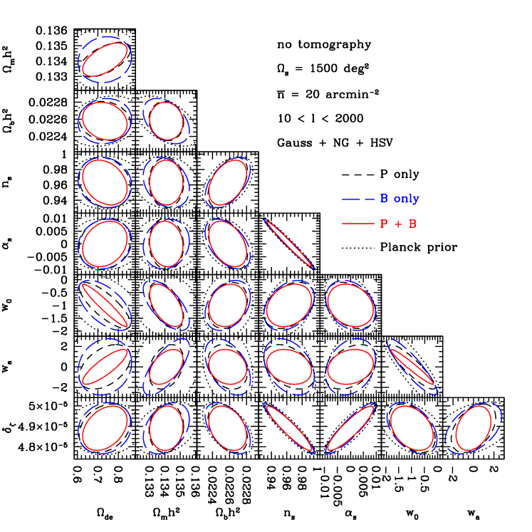
Figure 1: Fisher-forecasted error ellipses in each two-parameter subspace, marginalized over other parameters. The dotted contours are for the Planck-type CMB information alone. The other contours are the results expected when combining the CMB information with either of the lensing power spectrum (dashed, labelled as “P only”) or the bispectrum (long-dashed, “B only”) alone or the joint measurement (solid, “P+B”), where we employed $\Omega_{\rm s}=1500~{}$deg², $\bar{n}_{g}=20~{}$arcmin^-2, and $\langle z\rangle=1$ for survey parameters of the hypothetical Subaru HSC survey. We include the lensing information over the range of multipole, $10\leq l\leq 2000$, and do not include lensing tomography, i.e. consider one redshift bin of source galaxies.

Fig. 1 shows how the lensing power spectrum and bispectrum information lift parameter degeneracies in the Planck CMB information for the hypothetical Subaru HSC survey. For this plot, we did not include lensing tomography information, i.e. 1 redshift bin. Adding the lensing bispectrum information to the power spectrum tightens the error ellipses in each two-parameter sub-space, meaning that the lensing bispectrum does carry complementary information on cosmological parameters to the power spectrum. The lensing information leads to a significant improvement in the dark energy parameters ($\Omega_{\rm de},w_{0},w_{a}$), because the parameters are sensitive to the growth of structure formation from the CMB redshift to low redshifts, while the primary CMB information cannot well constrain the parameters. The other parameters such as the primordial power spectrum parameters are well constrained by the CMB information.

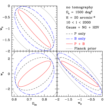
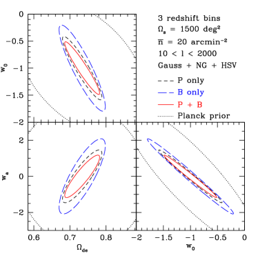
Figure 2: Left panel: Similar to the previous plot, but only for dark energy parameters ($\Omega_{\rm de},w_{0},w_{a}$). Right panel: Similar plots, but with lensing tomography of three redshift bins.

In Table 2 we show how lensing tomography improves constraints on dark energy parameters around the fiducial model (the cosmological constant model). The parameter constraints are improved by adding tomographic redshift information as well as adding the bispectrum information. To quantify the accuracy of dark energy parameters, we employ the DETF dark energy figure-of-merit (FoM) in Albrecht et al. (2006): FoM$\equiv 1/[\sigma(w_{\rm pivot})\sigma(w_{a})]$. Here $w_{\rm pivot}$ is the dark energy equation of state parameter at pivot redshift $z_{\rm pivot}$ and is defined in such a way that the errors in $w_{\rm pivot}$ and $w_{a}$ for given observables are uncorrelated. The error in $w_{\rm pivot}$ can be computed from the sub-matrix of the inverted Fisher matrix that contains only the elements of $w_{0}$ and $w_{a}$ (see Hu & Jain, 2004, for the definition). Table 2 shows that the three redshift-bin tomography allows for FoM$\simeq 30$ when combining the lensing power spectrum and bispectrum information, a factor of 10 or 5 improvement compared to FoM$\simeq 2.7$ or $6.4$ for the power spectrum alone or the joint measurement without tomography information, respectively. Comparing the results for the power spectrum alone and the joint measurement shows that adding the bispectrum tomography yields about 60–80% improvement for the 2 and 3 redshift-bin tomography cases. Since the dark energy FoM roughly scales with survey area as FoM$\propto\Omega_{\rm s}$, the improvement is equivalent to 1.6–1.8 larger survey area if using the power spectrum information alone. Fig. 2 visualizes the improvement of constraints on the dark energy parameters by adding the tomographic bins and the bispectrum information; considering multiple tomographic bins greatly improves the constrains, while the relative impact of adding the bispectrum becomes less prominent.

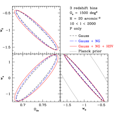
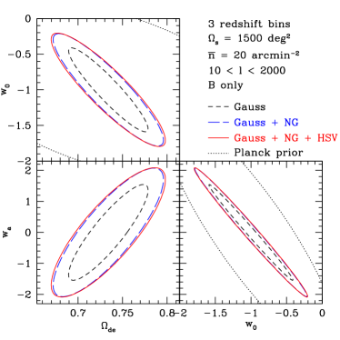
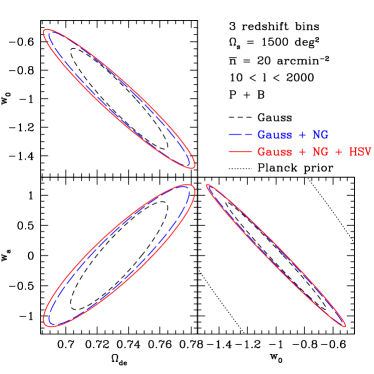
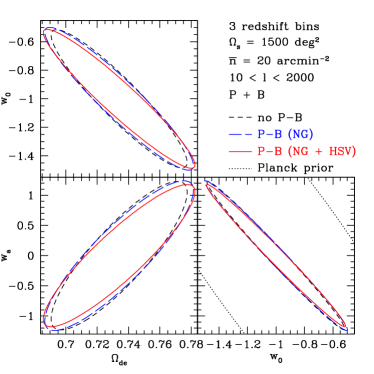
Figure 3: The impact of non-Gaussian error covariance on the marginalized errors of the dark energy parameters. We consider the cases with three tomographic redshift bins. Upper-left panel: The result obtained when including the power spectrum tomography alone. The solid curves are our fiducial results using the full covariance matrix of power spectrum, as we have shown in main text, while the dashed lines show the results obtained by assuming the Gaussian covariance matrix, i.e. ignoring the non-Gaussian errors, as done in Takada & Jain (2004). The long-dashed curves are with non-Gaussian covariance, but ignoring the HSV contribution. Upper-right and lower-left panels: Similar plots, but for the bispectrum and the joint measurement, respectively. Lower-right panel: The impact of the cross-covariance matrix between the power spectrum and bispectrum. We include the full covariance elements for the power spectrum and the bispectrum, but take different treatments for the cross-covariance matrix calculation. The solid contours are our fiducial results, i.e. including the full covariance. The short-dashed contours, labelled “no P-B”, are the results when ignoring the cross-covariance, i.e. no-correlation between the power spectrum and bispectrum. The dashed contours, labelled as “P-B (NG)”, are the results when including the cross-covariance matrix, but ignoring the HSV contribution.

In Fig. 3 we study the impact of non-Gaussian errors on the dark energy parameters. The figure shows how the error ellipses change if we ignore the non-Gaussian errors (i.e. assuming the Gaussian error covariances), the HSV contribution to the non-Gaussian errors, or the cross-covariance between the power spectrum and the bispectrum. Since the lensing power spectrum and bispectrum arise from the same large-scale structure in the light-cone volume, the two are highly correlated with each other. Comparing the top-left and -right panels reveals that the non-Gaussian errors yield a more significant degradation in the parameters for the bispectrum tomography than for the power spectrum. Although the HSV effect causes a significant degradation in the information content of the power spectrum or the bispectrum as carefully studied in Kayo et al. (2013), the impact on the parameter errors is modest after marginalizing over other parameters. To be more precise, the HSV effect enlarges a volume of the Fisher error ellipse in 8 dimensional parameter space by a factor of 2 compared to the case of ignoring the HSV effect, while the projected error for a particular parameter is enlarged only by about 10% ($\sim$ 2^1/8; see also Takada & Jain, 2009, for a similar discussion).

The results in Table 2 and Fig. 2 can be compared with Table 1 and Fig. 7 in Takada & Jain (2004). Our results show that adding the bispectrum information to the power spectrum gives a modest improvement, 10-20% for each dark energy parameter, while the latter found about 50% improvement. There are two important differences in between this work and Takada & Jain (2004). First, we have properly taken account of the non-Gaussian error covariances to perform the parameter forecasts, while Takada & Jain (2004) considered only the Gaussian covariance and included the information up to $l_{\rm max}=3000$ instead of 2000. The non-Gaussian error degrades the parameter errors. To be more explicit, if assuming the Gaussian covariance alone for 3 redshift-bin tomography, the power spectrum, the bispectrum and the joint measurement yield the marginalized errors of $\sigma(w_{0})=0.37$, $0.39$ and $0.23$ ($38\%$) and $\sigma(w_{a})=0.94$, 1.0, and $0.59$ (37%), respectively, which can be compared with Table 2. Second, we employ the primordial curvature perturbation for the normalization of the linear matter power spectrum, while Takada & Jain (2004) used the $\sigma_{8}$ normalization. When using the $\sigma_{8}$ normalization instead of $\delta_{\zeta}$, the weak lensing information primarily constrains not only the dark energy parameters $(\Omega_{\rm de},w_{0},w_{a})$, but also $\sigma_{8}$; that is, the CMB priors are less important for these parameters, because the parameters are sensitive to the growth of structure at low redshifts. Hence, adding the bispectrum more efficiently lifts parameter degeneracies in the four parameters, yielding a relatively greater improvement in each dark energy parameter compared to the power spectrum alone. In fact, we checked that our code fairly well reproduces the results in Takada & Jain (2004) if we follow the setting of Takada & Jain (2004): the $\sigma_{8}$ normalization, the Gaussian covariance, $l_{\rm max}=3000$ for the maximum multipole and the same survey parameters. This is encouraging because the details of model ingredients differ in the two studies. For example, we used the CAMB to compute the transfer function, while Takada & Jain (2004) used the BBKS transfer function (Bardeen et al., 1986). In addition, we used the halo model to compute the nonlinear bispectrum, while Takada & Jain (2004) employed the hyper extended perturbation theory (Scoccimarro & Couchman, 2001). The results in this paper are also consistent with the results in the early phase of this project, where the calculation was done using the completely different codes. Thus we believe that our results capture the genuine power of the lensing bispectrum for constraining cosmological parameters relative to the power spectrum.

However, we should note that our parameter forecasts are quite different from the recent result in Sato & Nishimichi (2013). The study fully relied on the ray-tracing simulations to compute the lensing power spectrum, the lensing bispectrum and their response to each cosmological parameter. They showed rather surprising results. For instance, the dark energy FoM for the lensing bispectrum tomography is greater than that of the power spectrum tomography, meaning that the lensing bispectrum is more powerful than does the power spectrum. They also argued that adding the bispectrum information yields a factor 2–3 improvement in each cosmological parameter compared to the power spectrum alone. Their results imply that the four-point function or the trispectrum can be even more important than the bispectrum and the power spectrum. We do not know where the big differences come from, so a further study is definitely needed.

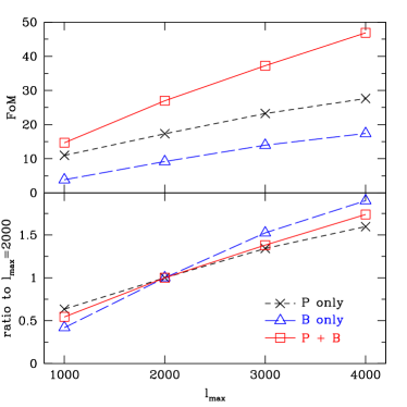
Figure 4: Upper panel: The dark energy FoM as a function of the maximum multipole $l_{\rm max}$, for the power spectrum (P), the bispectrum (B) and the joint experiment with 3 redshift-bin tomography, for a Subaru HSC-type survey as in Fig. 2. Note that we included the information over $10\leq l\leq l_{\rm max}$. With increasing $l_{\rm max}$, adding the bispectrum yields a greater improvement in the FoM compared to that of the power spectrum tomography alone. Lower panel: The degradation or improvement relative to the fiducial case of $l_{\rm max}=2000$.

We also consider some cases where the bispectrum tomography increases its relative importance for the parameter estimation. For instance, Table 3 compares the forecasts for the HSC- and Euclid-type surveys. Here we assume a lower mean redshift for the Euclid-type survey, $\langle z_{s}\rangle=0.7$, compared to $\langle z_{s}\rangle=1$ for the HSC-type survey. The weak lensing from a shallower survey probes large-scale structure at lower redshifts, where the large-scale structure is more evolved and shows stronger non-Gaussianity. Hence, the lensing bispectrum becomes more powerful for a shallower survey. Another example is in Fig. 4, which shows how the dark energy FoM is improved by including the power spectrum and bispectrum information up to higher $l_{\rm max}$, for a Subaru HSC-type survey. Here we consider the values of $l_{\rm max}=1000,2000,3000$ and $4000$. The weak lensing field at higher multipoles is more non-Gaussian, and therefore the lensing bispectrum brings stronger complementarity to the dark energy parameters.

4 Conclusion and Discussion

In this paper, we have extended the halo model based method in Kayo et al. (2013) to model the covariance matrices for the weak lensing power spectrum and bispectrum when tomographic redshift information is included. Then we have used the covariance formula to estimate a genuine power of the lensing bispectra, full the three-point correlation information, for constraining cosmological parameters when combined with the power spectrum information, for upcoming weak lensing surveys. To do this, we included all the bispectrum information built from all-available combinations of different redshift bins and different triangle configurations. Thus our study gives an answer on the best-available complementary information of the three-point correlation based statistics of weak lensing relative to the two-point correlation information, the power spectrum. Any collapsed three-point statistics such as skewness or a partial set of bispectra does not carry as much cosmological information as what we have shown in this paper.

We have shown that adding the bispectrum information helps to lift parameter degeneracies that appear when using the power spectrum information alone, with the CMB priors (see Figs. 1 and 2 and Tables 2 and 3). The parameter accuracy from the bispectrum information is more degraded by the non-Gaussian errors than that from the power spectrum (see Fig. 3). This result would be natural. The weak lensing power spectrum is primarily sensitive to cosmological parameters and carries the largest amount of information on the underlying matter distribution, because large-scale structure originates from the initial Gaussian field. The bispectrum is a measure of the non-Gaussian features in late-time large-scale structure that arise from the nonlinear clustering. In addition, there are too many different bispectra constructed from the range of multipoles. If assuming the Gaussian error covariances, it ignores correlations between the bispectra of different configurations. Hence it would be natural that the bispectrum is more affected by the non-Gaussian errors. When adding tomographic redshift information, improvements in parameter estimation by adding the bispectrum information become less significant compared to the improvement without tomography. Nevertheless, the joint measurement of the power spectrum and bispectrum for 3 redshift-bin tomography gives about 60% improvement in the dark energy FoM compared to the power spectrum tomography alone, for a Subaru HSC-type survey. This is promising in a sense that the improvement is equivalent to a factor 1.6 larger survey area if using the power spectrum alone. However, the power of lensing bispectrum is not as significant as what was claimed in Takada & Jain (2004), where a factor 2–3 improvement was found using the Gaussian covariance. Our results imply that even higher-order functions such as the four-point correlation function bring less complementary information than does the bispectrum. For a shallower weak lensing survey that preferentially probes the more evolving large-scale structure at lower redshift, the bispectrum becomes relatively more powerful to constrain parameters (see Table 3). For the same reason, when including the bispectrum up to the higher maximum multipole $l_{\rm max}$, the bispectrum becomes more useful (Fig. 4).

The bispectrum depends on cosmological parameters in a different way from the power spectrum. For instance, the lensing bispectrum is proportional to the cube of the lensing efficiency function, while the power spectrum is proportional to the square of the lensing efficiency function. Further, the lensing bispectrum is more sensitive to large-scale structure at lower redshifts than is the power spectrum, as we discussed. This is the main reason why adding the bispectrum information to the power spectrum allows for breaking parameter degeneracies. This complementarity would also be true for systematic errors inherent in weak lensing measurements such as photometric redshift errors and imperfect shape measurements; the power spectrum and bispectrum depend on the systematic errors in different ways. Hence, in the presence of systematic errors, adding the bispectrum information would allow for not only improving parameter estimations, but also calibrate out the systematic errors – self-calibration from the same data sets (Huterer et al., 2006). The self-calibration issue is worth exploring, and will be our future study.

The formulation developed in this paper would have various applications. It would be interesting to study even higher-order functions such as the trispectrum and then study how much complementary information is further added by them, compared to the power spectrum and bispectrum. The method shown in this paper can be easily extended to the trispectrum calculations. The abundance of massive halos are also complementary to the weak lensing information. In particular, the abundance of massive halos are affected by the same super-survey modes, through the HSV effect, so combining the weak lensing correlations with the abundance of massive halos in the same survey region can be used to correct for the HSV contamination. As we have shown, it is very important to take into account the covariance matrices between the different $n$-point correlations in order to properly count their independent information. Another promising weak lensing statistics is the cross-correlation of galaxy shapes with positions of foreground lensing objects (galaxies or clusters) with known redshifts – the so-called galaxy-galaxy lensing or cluster-galaxy lensing (Oguri & Takada, 2011; Okabe et al., 2013). The cross-correlation can probe the matter distribution at a particular redshift, the lensing redshift, i.e. free of the projection effect of large-scale structures at different redshifts along the line-of-sight direction. Most previous work has focused on the two-point correlation functions, but it would be worth further studying the three-point cross-correlation functions such as the halo-halo-shear or halo-shear-shear cross-correlations. Then, by fully taking into account the covariance matrices between the different cross-correlations, we can estimate the genuine power of the cross-correlation methods at two- and three-point level for constraining cosmology. For these studies, the method and formulation in this paper would be useful. These are our future subjects, and will be presented elsewhere.

References

- Albrecht et al. (2006) Albrecht A. et al., 2006, ArXiv Astrophysics e-prints
- Bardeen et al. (1986) Bardeen J. M., Bond J. R., Kaiser N., Szalay A. S., 1986, ApJ, 304, 15
- Bartelmann & Schneider (2001) Bartelmann M., Schneider P., 2001, Phys. Rep., 340, 291
- Bergé et al. (2010) Bergé J., Amara A., Réfrégier A., 2010, ApJ, 712, 992
- Bernardeau et al. (2002) Bernardeau F., Colombi S., Gaztañaga E., Scoccimarro R., 2002, Physics Report, 367, 1
- Bernardeau et al. (2002) Bernardeau F., Mellier Y., van Waerbeke L., 2002, A&A, 389, L28
- Bernardeau et al. (1997) Bernardeau F., van Waerbeke L., Mellier Y., 1997, A&A, 322, 1
- Cooray & Hu (2001a) Cooray A., Hu W., 2001a, ApJ, 554, 56
- Cooray & Hu (2001b) Cooray A., Hu W., 2001b, ApJ, 548, 7
- Cooray & Sheth (2002) Cooray A., Sheth R., 2002, Physics Report, 372, 1
- Dodelson & Zhang (2005) Dodelson S., Zhang P., 2005, Phys. Rev. D, 72, 083001
- Hamana & Mellier (2001) Hamana T., Mellier Y., 2001, MNRAS, 327, 169
- Hamana et al. (2003) Hamana T. et al., 2003, ApJ, 597, 98
- Hamilton et al. (2006) Hamilton A. J. S., Rimes C. D., Scoccimarro R., 2006, MNRAS, 371, 1188
- Harnois-Déraps et al. (2012) Harnois-Déraps J., Vafaei S., Van Waerbeke L., 2012, MNRAS, 426, 1262
- Heymans et al. (2013) Heymans C. et al., 2013, MNRAS
- Hoekstra & Jain (2008) Hoekstra H., Jain B., 2008, Annual Review of Nuclear and Particle Science, 58, 99
- Hu (1999) Hu W., 1999, ApJ, 522, L21
- Hu & Jain (2004) Hu W., Jain B., 2004, Phys. Rev. D, 70, 043009
- Hu & Kravtsov (2003) Hu W., Kravtsov A. V., 2003, ApJ, 584, 702
- Hui (1999) Hui L., 1999, ApJ, 519, L9
- Huterer (2002) Huterer D., 2002, Phys. Rev. D, 65, 063001
- Huterer & Takada (2005) Huterer D., Takada M., 2005, Astroparticle Physics, 23, 369
- Huterer et al. (2006) Huterer D., Takada M., Bernstein G., Jain B., 2006, MNRAS, 366, 101
- Jain & Khoury (2010) Jain B., Khoury J., 2010, Annals of Physics, 325, 1479
- Jain & Seljak (1997) Jain B., Seljak U., 1997, ApJ, 484, 560
- Jain et al. (2000) Jain B., Seljak U., White S., 2000, ApJ, 530, 547
- Jarvis et al. (2004) Jarvis M., Bernstein G., Jain B., 2004, MNRAS, 352, 338
- Kayo et al. (2013) Kayo I., Takada M., Jain B., 2013, MNRAS, 429, 344
- Kilbinger et al. (2013) Kilbinger M. et al., 2013, MNRAS, 430, 2200
- Kilbinger & Schneider (2005) Kilbinger M., Schneider P., 2005, A&A, 442, 69
- Komatsu et al. (2011) Komatsu E. et al., 2011, ApJS, 192, 18
- Lewis et al. (2000) Lewis A., Challinor A., Lasenby A., 2000, ApJ, 538, 473
- Limber (1954) Limber D. N., 1954, ApJ, 119, 655
- Ma & Fry (2000) Ma C., Fry J. N., 2000, ApJ, 543, 503
- Miyazaki et al. (2012) Miyazaki S. et al., 2012, in Society of Photo-Optical Instrumentation Engineers (SPIE) Conference Series.
- Mo et al. (1997) Mo H. J., Jing Y. P., White S. D. M., 1997, MNRAS, 284, 189
- Mo & White (1996) Mo H. J., White S. D. M., 1996, MNRAS, 282, 347
- Munshi et al. (2011) Munshi D., Kitching T., Heavens A., Coles P., 2011, MNRAS, 416, 1629
- Navarro et al. (1997) Navarro J. F., Frenk C. S., White S. D. M., 1997, ApJ, 490, 493
- Oguri & Takada (2011) Oguri M., Takada M., 2011, Phys. Rev. D, 83, 023008
- Okabe et al. (2013) Okabe N., Smith G. P., Umetsu K., Takada M., Futamase T., 2013, ApJ, 769, L35
- Peacock & Smith (2000) Peacock J. A., Smith R. E., 2000, MNRAS, 318, 1144
- Pires et al. (2012) Pires S., Leonard A., Starck J.-L., 2012, MNRAS, 423, 983
- Planck Collaboration et al. (2013) Planck Collaboration et al., 2013, ArXiv e-prints
- Sato et al. (2009) Sato M., Hamana T., Takahashi R., Takada M., Yoshida N., Matsubara T., Sugiyama N., 2009, ApJ, 701, 945
- Sato & Nishimichi (2013) Sato M., Nishimichi T., 2013, ArXiv e-prints
- Sato et al. (2011) Sato M., Takada M., Hamana T., Matsubara T., 2011, ApJ, 734, 76
- Schneider (2006) Schneider P., 2006, in Meylan G., Jetzer P., North P., Schneider P., Kochanek C. S., Wambsganss J., eds, Saas-Fee Advanced Course 33: Gravitational Lensing: Strong, Weak and Micro. pp 269–451
- Schrabback et al. (2010) Schrabback T. et al., 2010, A&A, 516, A63
- Scoccimarro & Couchman (2001) Scoccimarro R., Couchman H. M. P., 2001, MNRAS, 325, 1312
- Scoccimarro et al. (2001) Scoccimarro R., Sheth R. K., Hui L., Jain B., 2001, ApJ, 546, 20
- Scoccimarro et al. (1999) Scoccimarro R., Zaldarriaga M., Hui L., 1999, ApJ, 527, 1
- Seljak (2000) Seljak U., 2000, MNRAS, 318, 203
- Semboloni et al. (2008) Semboloni E., Heymans C., van Waerbeke L., Schneider P., 2008, MNRAS, 388, 991
- Semboloni et al. (2011) Semboloni E., Schrabback T., van Waerbeke L., Vafaei S., Hartlap J., Hilbert S., 2011, MNRAS, 410, 143
- Semboloni et al. (2007) Semboloni E., van Waerbeke L., Heymans C., Hamana T., Colombi S., White M., Mellier Y., 2007, MNRAS, 375, L6
- Sheth & Tormen (1999) Sheth R., Tormen G., 1999, MNRAS, 308, 119
- Spergel et al. (2013) Spergel D. et al., 2013, ArXiv e-prints
- Takada & Bridle (2007) Takada M., Bridle S., 2007, New Journal of Physics, 9, 446
- Takada & Hu (2013) Takada M., Hu W., 2013, Phys. Rev. D, 87, 123504
- Takada & Jain (2002) Takada M., Jain B., 2002, MNRAS, 337, 875
- Takada & Jain (2003a) Takada M., Jain B., 2003a, MNRAS, 340, 580
- Takada & Jain (2003b) Takada M., Jain B., 2003b, MNRAS, 344, 857
- Takada & Jain (2004) Takada M., Jain B., 2004, MNRAS, 348, 897
- Takada & Jain (2009) Takada M., Jain B., 2009, MNRAS, 395, 2065
- Takada et al. (2006) Takada M., Komatsu E., Futamase T., 2006, Phys. Rev. D, 73, 083520
- Takahashi et al. (2012) Takahashi R., Sato M., Nishimichi T., Taruya A., Oguri M., 2012, ApJ, 761, 152
- Takahashi et al. (2009) Takahashi R. et al., 2009, ApJ, 700, 479
- Van Waerbeke et al. (2001) Van Waerbeke L., Hamana T., Scoccimarro R., Colombi S., Bernardeau F., 2001, MNRAS, 322, 918
- Weinberg et al. (2012) Weinberg D. H., Mortonson M. J., Eisenstein D. J., Hirata C., Riess A. G., Rozo E., 2012, ArXiv e-prints
- White & Hu (2000) White M., Hu W., 2000, ApJ, 537, 1
- Zhang et al. (2003) Zhang T.-J., Pen U.-L., Zhang P., Dubinski J., 2003, ApJ, 598, 818