The Academic Social Network

Abstract

Through academic publications, the authors of these publications form a social network. Instead of sharing casual thoughts and photos (as in Facebook), authors pick co-authors and reference papers written by other authors. Thanks to various efforts (such as Microsoft Libra and DBLP), the data necessary for analyzing the academic social network is becoming more available on the Internet. What type of information and queries would be useful for users to find out, beyond the search queries already available from services such as Google Scholar? In this paper, we explore this question by defining a variety of ranking metrics on different entities - authors, publication venues and institutions. We go beyond traditional metrics such as paper counts, citations and h-index. Specifically, we define metrics such as influence, connections and exposure for authors. An author gains influence by receiving more citations, but also citations from influential authors. An author increases his/her connections by co-authoring with other authors, and specially from other authors with high connections. An author receives exposure by publishing in selective venues where publications received high citations in the past, and the selectivity of these venues also depends on the influence of the authors who publish there. We discuss the computation aspects of these metrics, and similarity between different metrics. With additional information of author-institution relationships, we are able to study institution rankings based on the corresponding authors’ rankings for each type of metric as well as different domains. We are prepared to demonstrate these ideas with a web site (http://pubstat.org) built from millions of publications and authors.

1 Introduction

In the academic community, it is customary to get a quick impression of an author’s research from simple statistics about his/her publications. Such statistics include paper count, citations of papers, h-index and various other indices for counting papers and citations. Several services, such as ISI, Scopus, Google Scholar, CiteSeerX Giles et al (1998), DBLP Ley (2009) and Microsoft Libra (2013), facilitate the retrieval of these statistics by maintaining databases indexing the metadata of academic publications. These databases are usually proprietary and the information users can retrieve, sometimes on a paid basis, is limited to what these services choose to provide.

In recent years, some of these service providers Ley (2009); Libra (2013) are making the database more publically accessible and are starting to provide additional information users can query (this is specially the case with Libra). This allows us to study the author community as a social network, analyzing not only the statistics about papers published by an author, individually at a time, but also an author’s choice and extent in connecting to other authors (co-authoring) and an author’s influence on other authors. Since citation is a slow indicator for evaluating an author’s standing, we can also design metrics to measure an author’s exposure in her research community, to estimate his/her future influence and connections in research.

Our approach is to design various social network types of metrics to measure the traits defined above. Since there is no ground-truth for validation, we justify our designs by the following methods: (1) Compare top ranked authors to those receiving awards for qualities similar to what we try to measure, e.g. influence; (2) Use similarity study to ensure any new metric can measure something different from that is indicated by other well-established metrics already; (3) Undertake case-studies of those authors scoring very differently under different metrics, in domains we are familiar with; (4) Let colleagues use our experimental website (http://pubstat.org) and get their feedback on its usefulness.

Our conclusion is that several of the metrics we designed, namely Influence, Connections and Exposure, can provide different rankings of authors, and together with Citation Count can give a fuller picture about authors.

According to the author ranking results, combined with additional information on author-institution relationships, we further studied and designed approaches for conducting author-based institution ranking for each of the various metrics as well as the subject domains.

In the rest of the paper, we first describe briefly the available dataset. We then describe the metrics we studied and the ranking services we built. Next we evaluate our metrics and ranking methods using the approach described above. We finish by discussing related works and our conclusions.

2 Data

Our data is collected from the Microsoft Libra public API. The Libra data has an object-level organization Nie et al (2007), which is very helpful. The object type includes: author, paper, conference venue, institution and so on. Each type of object possess general properties such as a unique identifier, name and relationship to other objects. For example, if the object is a paper, then its properties include publication year, authorship and citations. In fact, Libra has maintained a huge amount of data in a very wide range of research fields (15) and, for each field, it further categorizes the papers to belong to domains in that field. The data set we obtained for experimental purposes was for the Computer Science field, which included 24 domains. Table 1 lists the name, the number of authors and the number of papers in the domains. Since each author may publish papers in different domains, the sum of authors in all domains is significantly greater than the number of unique authors (941733). The number of papers in the database (3347795) is actually significantly greater than the sum from all domains (2449673). This is because many papers were not classified or had missing information. Another fact we needed to consider was that an increasing proportion of these papers were published in more recent years, as shown in Fig. 1. This has some ramifications for our analysis, as we discuss in the latter part of this paper. Despite the misgivings about the dataset we make many interesting observations.

Table 1: The basic information of the Libra dataset we use: domain name, the number of authors and the number of papers in each of the 24 domains of the Computer Science Area.

Domain Name	#Authors	#Papers
Algorithms and Theory	96748	270601
Security and Privacy	33910	61957
Hardware and Architecture	81021	150151
Software Engineering	85938	174893
Artificial Intelligence	186976	325109
Machine Learning and Pattern Recognition	66839	108234
Data Mining	50958	67485
Information Retrieval	30038	51075
Natural Language and Speech	86670	220227
Graphics	36548	59880
Computer Vision	44969	60806
Human-Computer Interaction	51548	79909
Multimedia	59277	80618
Network and Communications	138096	235297
World Wide Web	25098	35861
Distributed and Parallel Computing	69592	117836
Operating System	18167	25395
Databases	74125	142421
Real-Time and Embedded System	21965	33098
Simulation	18083	27678
Bioinformatics and Computational Biology	48729	55491
Scientific Computing	103982	183878
Computer Education	29420	49125
Programming Languages	33229	70561
Computer Science Overall (24 domains)	941733	2449673
Computer Science Total Involved	1175052	3347795

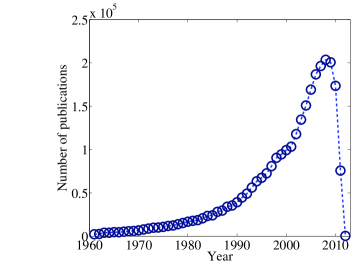
Figure 1: The number of papers in the Libra CS domain changing with time.

3 Metrics and Ranking Methods

3.1 Metrics

All the metrics we studied can be defined by considering three types of object: (a) papers, (b) authors and (c) venues. The relationships between these objects are captured by the following networks (graphs):

1. paper citation network, denoted by $G_{P}=(V_{P},E_{P})$, where $V_{P}$ is the set of papers and $E_{P}$ is the set of citations from one paper to another.
   

2. authorship bipartite network, denoted by $G_{AP}=(V_{A}\cup V_{P},E_{AP})$, where $V_{A}$ is the set of authors and edges in the set $E_{AP}$ link each paper to its authors (authorship) and symmetrically each author to his/her publications (ownership).
   

3. venueship bipartite network, denoted by $G_{VP}=(V_{V}\cup V_{P},E_{VP})$, where $V_{V}$ is the set of venues and the edges in $E_{VP}$ connect each paper to its publishing venue. Topologically, $G_{VP}$ is similar to $G_{AP}$. The main difference is that each paper can have multiple authors while it can only be published in one venue.

Fig. 2 shows the super-graph $G=(V,E)$ combining all three networks together. In this case, $V=(V_{P}\cup V_{A}\cup V_{V})$ and $E=(E_{P}\cup E_{AP}\cup E_{VP})$.

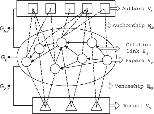
Figure 2: Underlay network topology of authors, venues and papers.

We also denote $n_{A}=|V_{A}|,n_{V}=|V_{V}|$ and $n_{P}=|V_{P}|$ as the number of authors, venues and papers, respectively.

We grouped the metrics we defined into three categories. A metric may be a simple count, such as citation count, or a value derived iteratively using a PageRank-like algorithm.

1. Paper based - In this case, each paper has a value defined by a metric. The value is distributed to the paper’s authors in a way also determined by the metric. For this category, we studied three metrics: Citation count (CC), Balanced citation count (BCC) and Citation value (CV). For CC and BCC, the paper’s value was simply the citation count, which is well-defined. In CC’s case, each co-author received the citation count whereas in BCC’s case, each co-author only received an equal fraction of the citation count. For CV, it was computed iteratively based on the citation graph $G_{P}$ and distributed to the co-authors in equal fractions.
   

2. Author based - These metrics were computed based on author-to-author relationships directly. In this category, we studied three metrics: Influence, Followers and Connections. All three were computed iteratively. For Influence, the author-to-author relationship was derived from the citation graph $G_{P}$ and authorship graph $G_{AP}$. Every time author $i$ cites author $j$’s paper, author $i$’s Influence was distributed to author $j$, split among the co-authors of $j$. For Followers, the author-to-author relationship was also derived from the citation graph, but depended on whether author $i$ cited author $j$ instead of how many times. If author $i$ cited author $j$, author $i$’s Follower value was distributed to author $j$ without splitting among author $j$’s co-authors (which could be different for different papers). The author-to-author relationship for Connections was defined only based on the authorship graph $G_{AP}$. If author $i$ had co-authored a paper with author $j$, then author $i$’s Connections value was distributed to author $j$ and vice versa. Note, another variation of Connections could also be defined so that every time author $i$ co-authored with author $j$, they exchanged their Connections value.
   

3. Author and venue based - In this category, we defined only one metric: Exposure. This metric was computed by iterating on authors and venues together. It is easiest to think of venues also as a kind of author, thus we had an enlarged author set $V_{A}\cup V_{V}$. The author-to-author relationship was defined in the same way as Influence; so was the relationship for venue-to-venue. The author-to-venue and venue-to-author relationships were defined intuitively as follows: each time an author $i$ wrote a paper published in venue $k$, author $i$ distributed his/her influence to venue $k$; similarly, each time a venue $k$ published a paper co-authored by $i$, author $i$ shared a fraction of venue $k$’s influence with $i$’s co-authors for that paper.

Note, all these (7) metrics were defined so as to assign a value to each author, to indicate some characteristics of that author. Since citation count (CC) could be inflated by a large number of co-authored papers, BCC and CV were alternative computations to assign citation credits to authors. The metrics Influence and Followers are intended to characterize an author’s influence and impact on other authors. The metric Connections is used to measure an author’s reach in the co-authorship network. Finally, Exposure is intended to bring in the impact of the venues to help characterize an author’s potential influence that may not be reflected by citations if the author’s papers were relatively recent.

For a precise definition of the above metrics, it is necessary to explain the PageRank algorithm. A brief treatment of PageRank and the metrics definition by equations are included in the Appendix.

3.2 Ranking

Given the metrics we defined, we computed for each author his/her ranking for each metric. An example of an author ”J Smith” (with the actual name anonymized) returned by our web service is listed in Table 2:

Table 2: An example of the different metric results returned by our web service in the “Network and Communications” domain with actual author name anonymized.

Value Type	Author	CC	BCC	CV	Inf	Fol	Con	Exp
Rank	J Smith	4786	2483	2996	4100	7647	2820	1805
RankPer	J Smith	$3.47\%$	$1.8\%$	$2.17\%$	$2.97\%$	$5.54\%$	$2.04\%$	$1.31\%$
CumValue	J Smith	72.25%	63.66%	58.45%	56.49%	59.51%	18.15%	26.91%

Actually, this ranking is for a specific domain (“Network and Communications”) which has close to 138K authors in our database. So this author is ranked well within the top ten percentile of this domain he/she works in. In order to give this information, we also allow the user to view the ranking in terms of percentile (denoted by RankPer, the 3rd row in Table 2).

A third choice is to view the ranking information in terms of the cumulative value of contribution by authors ranked ahead of the target author (denoted by CumValue, the 4th row in Table 2).

Finally, we considered it more appropriate to use a coarse granularity for such ranking information (especially applied in the case study in a later section). There were two possible ways: (1) based on cumulative value of contribution; (2) based on rank percentile.

Contribution based letter grading:

for this purpose, we decided to divide the cumulative value range into five fixed intervals, and assign letter grade ABCDE as ranks. Lacking any better way to calibrate the partitioning, we simply used 20%, 40%, 60% and 80% as the thresholds. In this view, the above example becomes (Table 3):

Table 3: Example of the contribution based letter grades for each metric, where A:$(0-20\%)$, B:$(20\%-40\%)$, C:$(40\%-60\%)$, D:$(60\%-80\%)$ and E:$(80\%-100\%)$

. Value Type Author CC BCC CV Inf Fol Con Exp CumValue J Smith 72.25% 63.66% 58.45% 56.49% 59.51% 18.15% 26.91% Contri. Letter J Smith D D C C D A B

For most metrics, the distribution of contribution by authors ordered according to ranking follows Pareto-like distribution. For example, Fig. 3 shows the relationship between the rank order to the cumulative value of three metrics, Influence, Connections and Exposure, using a loglog plot.

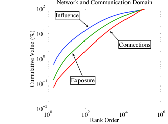
Figure 3: The loglog results of rank orders versus cumulative values of three metrics: Influence, Connections and Exposure.

So out of over 138K authors, the distribution of ABCDE for the different metrics are listed in Table 4.

Table 4: The distribution of contribution based letter assignment for different metrics of around 138k authors in “Network and Communications” domain of Libra dataset.

	CC	BCC	CV	Inf	Fol	Con	Exp
A	156	148	179	214	485	3386	940
B	558	513	752	994	1764	11516	3978
C	1629	1469	2366	4134	5646	32653	12251
D	5550	5059	9012	25916	26705	20866	31962
E	130203	130907	125787	106838	103496	69675	88965

Rank Percentile based letter grading:

An alternative way of letter assignment was based on rank percentile. Since the cumulative curves of the metrics show the power-law property, we thus proposed the power-based thresholds $(\alpha^{4},\alpha^{3},\alpha^{2},\alpha)$ to assign letters according to the rank percentile, where parameter $\alpha\in(0,1)$ controled the skewness of the assignment results. Table 5 illustrates the letter assignment results when we set $\alpha=0.25$ for the experimental web site.

Table 5: The illustration of power-based letter assignment according to the rank percentile with parameter $\alpha\in(0,1)$.

	Rank Percentile	$\alpha=0.25$
A	$(0-\alpha^{4})$	$(0-0.39\%)$
B	$(\alpha^{4}-\alpha^{3})$	$(0.39\%-1.56\%)$
C	$(\alpha^{3}-\alpha^{2})$	$(1.56\%-6.25\%)$
D	$(\alpha^{2}-\alpha)$	$(6.25\%-25\%)$
E	$(\alpha-1)$	$(25\%-100\%)$

The letter grades according to the rank percentile on the “J Smith” example are listed in Table 6.

Table 6: Letter grades for each metric by power-based assignment according to the rank percentile on the example “J Smith”, where $\alpha=0.25$.

Value Type	Author	CC	BCC	CV	Inf	Fol	Con	Exp
RankPer	J Smith	$3.47\%$	$1.8\%$	$2.17\%$	$2.97\%$	$5.54\%$	$2.04\%$	$1.31\%$
RankPer Letter	J Smith	C	C	C	C	C	C	B

It remains an open problem of how to find the best way of letter grades assignment, which we consider to be future work. We briefly discuss the pros and cons of the two letter assignment methods proposed by us, contribution based vs. rank percentile based.

One notable difference was the metric-dependency of the letter count distribution. By definition, rank percentile based letter grading results in a consistent letter count distribution among different metrics (hence independent of metrics). However, it varies a lot among different metrics for letter count distribution generated by contribution based letter grading. For example, as shown in Table 4, there were 156 “A”s for the Citation Count (CC) metric when 3386 “A”s for the Connection (Con) metric. This was caused by the different skewness in the value distribution of authors’ contribution for various metrics, which could also be inferred from the cumulative curves shown in Fig. 3.

On the other hand, any change in the total number of authors in a research domain (e.g. community expansion or rapid development) unavoidably affects the letter count distribution generated by rank percentile based letter grading, but it has very limited effects on the contribution based letter assignment results when the value distribution is very skewed (e.g. Influence etc.).

Later on, unless otherwise noted, we only show the letter assignment results by percentile based grading for space saving and fair comparison among various metrics.

3.3 Domain-specific vs Overall Ranking

As mentioned, the above example is the ranking for an author in a specific domain. Usually, an author works in several domains. Our web service shows the author’s rankings in all the domains, as well as an overall score for his/her subject field (in this case “Computer Science”). The letter grades of the example “J Smith” are listed in Table 7).

Table 7: Letter grades of each metric in several involved domains of the example “J Smith”.

Domain	CC	BCC	CV	Inf	Fol	Con	Exp
Net&Comm	C	C	C	C	C	C	B
Sec&Priv	D	D	D	D	E	E	D
Overall	C	C	C	C	C	C	B

This allows the person to be compared to others in his/her domain, as well as comparing him/her to a bigger set of people in a subject field.

The way to compute the overall score is difficult. We used the straightforward way of merging all the domains into one big domain and compared the results. This was more computationally demanding. Another possible way would be to add up the authors ranking in each domain normalized by the size of each domain. The trade-off of different ways for computing the overall is something still under study.

3.4 Comparing Rankings

In our experimental web site, we have implemented different ways for authors to be compared. First of all, authors in the same domain can be looked up in ranking order, according to any metric. So it would be easy to look up top-ranked people according to one’s favourite metric, whether it was Influence, Connections, or Exposure. This is often helpful.

Second, we allow authors in the same institution to be looked up in ranking order, for a specific domain, or according to overall ranking. This would be useful in getting a feel as to how strong a particular institute was in a particular domain. It is also the rough way we justify our assignment of ABCDE to authors in different cumulative value percentiles or rank percentiles.

We also allow users to search for individual authors and keep them in a list for head-to-head comparison. This could be helpful for many different purposes. For example, we could use this method to collect a list of authors for a case study (see next section).

We have also implemented various other features. For example, it would be possible to look at all rankings if we excluded self-citations. Basically, for each common query users find useful, we could implement it as an additional feature.

3.5 Author-based Institution Rankings

With the additional information of author-institution relationships, we can further provide institution rankings based on authors’ ranking results. When ranking institutions, we used two granularities:

1. We only count the number of authors assigned with “A”;

2. We compute a total score, counting “A”=1, “B”=0.5, “C”=0.25, and “D”=“E”=0.

For ranking authors, there are a number of various metrics (e.g., Influence, Connections, Exposure, etc.), two types of letter assignment (contribution based vs. rank percentile based) and the domain-specificity (e.g., 24 domains listed in Table 1), therefore the institution ranking automatically inherits these features.

4 Evaluation and Validation

4.1 Ranking Award Recipients

One way to justify our new metrics is to look at award recipients. In the computer science domain, the most prestigious award is the Turing Award. Since we are more familiar with the Network and Communications domain, we also looked at the ACM Sigcomm Award recipients. The results are shown in the following two tables (Table 8 and Table 9).

Table 8: Rankings received by Turing Award Recipients

Year	Awardee	In/All	h	CC	BCC	CV	Inf	Fol	Con	Exp	Aff
1966	Alan J. Perlis	31/47	9	B	B	B	A	A	C	B	Yale
1967	Maurice V. Wilkes	50/100	11	B	B	A	A	A	D	A	Cambridge
1968	Richard W. Hamming	9/29	8	B	A	A	A	A	E	B	Naval Postgraduate Sch.
1969	Marvin Minsky	50/79	20	A	A	A	A	A	D	A	MIT
1970	James H. Wilkinson	23/48	9	B	A	A	A	A	D	A	Nat. Physical Lab, UK
1971	John McCarthy	117/209	29	A	A	A	A	A	B	A	Princeton
1972	Edsger W. Dijkstra	84/121	28	A	A	A	A	A	C	A	UT Austin
1973	Charles W. Bachman	18/25	7	C	B	B	A	B	C	B	Bachman Info Systems
1974	Donald E. Knuth	179/241	40	A	A	A	A	A	B	A	Stanford
1975	Allen Newell	139/192	33	A	A	A	A	A	A	A	Carnegie Mellon Univ
	Herbert Simon	140/398	33	A	A	A	A	A	B	A	Illinois Institute of Tech
1976	Michael O. Rabin	68/81	28	A	A	A	A	A	C	A	Columbia
	Dana Stewart Scott	48/71	21	A	A	A	A	A	C	A	Carnegie Mellon Univ.
1977	John W. Backus	32/73	11	A	A	A	A	A	C	A	IBM
1978	Robert W. Floyd	36/46	16	A	A	A	A	A	D	A	Illinois Institute of Tech
1979	Kenneth E. Iverson	43/70	10	C	B	B	A	A	C	A	IBM
1980	C. A. R. Hoare	198/249	41	A	A	A	A	A	B	A	Microsoft Research
1981	Edgar Frank Codd	27/32	15	A	A	A	A	A	D	A	IBM
1982	Stephen A. Cook	127/138	32	A	A	A	A	A	B	A	Univ of Michigan
1983	Ken Thompson	26/51	13	A	A	A	A	A	C	A	Google
	Dennis M. Ritchie	29/37	15	A	A	A	A	A	D	A	Bell Labs
1984	Niklaus Emil Wirth	110/144	30	A	A	A	A	A	D	A	Xerox PARC
1985	Richard Manning Karp	277/325	61	A	A	A	A	A	A	A	IBM
1986	John Edward Hopcroft	147/176	39	A	A	A	A	A	B	A	Stanford
	Robert Endre Tarjan	338/362	72	A	A	A	A	A	A	A	Hewlett-Packard
1987	John Cocke	45/52	20	A	A	A	A	A	C	A	IBM
1988	Ivan E. Sutherland	57/63	21	A	A	A	A	A	B	A	Portland State Univ
1989	William Morton Kahan	32/39	11	C	C	B	B	B	B	C	UC Berkeley
1990	Fernando Jose Corbato	7/13	5	C	C	B	B	A	D	C	MIT
1991	Robin Milner	143/172	47	A	A	A	A	A	B	A	Cambridge
1992	Butler W. Lampson	116/140	36	A	A	A	A	A	B	A	MIT
1993	Juris Hartmanis	115/140	25	A	A	A	A	A	B	A	Cornell
	Richard Edwin Stearns	77/89	20	A	A	A	A	A	B	A	NY Univ at Albany
1994	Edward A. Feigenbaum	37/58	14	B	B	A	A	A	C	A	Stanford
	Raj Reddy	70/99	14	B	B	A	A	A	B	A	Cargegie Mellon Univ
1995	Manuel Blum	100/112	33	A	A	A	A	A	B	A	Carnegie Mellon Univ
1996	Amir Pnueli	331/371	62	A	A	A	A	A	A	A	New York Univ
1997	Douglas C. Engelbart	23/31	14	B	A	A	A	A	C	A	Doug Engelbart Institute
1998	Jim Gray	217/293	46	A	A	A	A	A	A	A	Microsoft Research
1999	Fred Brooks	77/112	21	A	A	A	A	A	A	A	UNC
2000	Andrew Chi-chih Yao	159/183	35	A	A	A	A	A	B	A	Tsinghua Univ
2001	Ole-johan Dahl	32/39	13	B	B	A	A	A	C	B	Univ of Oslo
	Kristen Nygaard	35/43	14	B	B	A	A	A	C	B	Univ of Oslo
2002	Ronald L. Rivest	226/267	52	A	A	A	A	A	A	A	MIT
	Adi Shamir	186/206	46	A	A	A	A	A	A	A	Weizmann Institute
	Leonard Max Adleman	72/86	27	A	A	A	A	A	B	A	MIT
2003	Alan Curtis Kay	22/33	7	B	B	B	B	B	C	B	Hewlett-Packard Labs
2004	Vinton Gray Cerf	39/56	10	B	B	B	A	A	B	B	Google
	Robert Elliot Kahn	15/23	9	C	C	A	A	A	C	B	CNRI
2005	Peter Naur	40/137	7	C	B	A	A	A	D	A	Univ of Copenhagen
2006	Frances E. Allen	26/37	14	B	B	A	A	A	C	B	IBM
2007	Edmund Clarke	333/370	63	A	A	A	A	A	A	A	Carnegie Mellon Univ
	E. Allen Emerson	132/150	41	A	A	A	A	A	B	A	UT Austin
	Joseph Sifakis	139/164	36	A	A	A	A	A	A	A	CNRS
2008	Barbara Liskov	195/233	48	A	A	A	A	A	A	A	MIT
2009	Charles P. Thacker	12/15	7	B	B	B	A	A	C	C	Microsoft
2010	Leslie Valiant	113/124	37	A	A	A	A	A	C	A	Harvard Univ
2011	Judea Pearl	193/258	39	A	A	A	A	A	B	A	UCLA
2012	Shafi Goldwasser	138/152	43	A	A	A	A	A	B	A	Weizmann Institute
	Silvio Micali	165/173	46	A	A	A	A	A	B	A	MIT

Table 9: Rankings received by Sigcomm Award recipients

Year	Awardee	In/All	h	CC	BCC	CV	Inf	Fol	Con	Exp	Aff.
1989	Paul Baran	1/7	1	D	D	C	C	C	E	D	RAND Corporation
1990	Leonard Kleinrock	173/233	31	A	A	A	A	A	A	A	UCLA
	David D. Clark	43/80	13	B	B	B	A	A	B	B	MIT
1991	Hubert Zimmermann	10/17	4	C	B	B	B	B	E	B	Sun Microsystems
1992	A. G. Fraser	16/24	6	C	C	B	A	B	E	B	Fraser Research
1993	Robert Elliot Kahn	15/23	9	C	C	A	A	A	C	B	CNRI
1994	Paul E. Green	20/54	7	C	B	B	B	B	C	B	Tellabs
1995	David J. Farber	43/55	13	B	B	B	B	A	B	B	Carnegie Mellon Univ
1996	Vinton Gray Cerf	39/56	10	B	B	B	A	A	B	B	Google
1997	Jonathan B. Postel	73/92	24	A	A	A	A	A	B	A	Univ of Southern California
	Louis Pouzin	7/23	3	D	C	B	B	B	E	C	ITU
1998	Lawrence G. Roberts	14/16	8	B	A	A	A	A	D	A	Anagran Inc.
1999	Peter T. Kirstein	45/67	7	C	C	B	B	B	C	B	Univ College London
2000	Andre A. S. Danthine	31/44	7	C	C	C	C	C	C	C	Université de Liége
2001	Van Jacobson	113/126	41	A	A	A	A	A	B	A	Palo Alto Research Center
2002	Scott J. Shenker	413/481	88	A	A	A	A	A	A	A	UC Berkeley
2003	David Cheriton	156/186	36	A	A	A	A	A	B	A	Stanford
2004	Simon Lam	148/181	30	A	A	A	A	A	B	A	UT Austin
2005	Paul V. Mockapetris	17/21	8	B	A	A	A	A	E	A	Nominum
2006	Domenico Ferrari	101/128	30	A	A	A	A	A	B	A	UC Berkeley
2007	Sally Floyd	186/206	59	A	A	A	A	A	A	A	ICSI
2008	Donald F. Towsley	618/725	65	A	A	A	A	A	A	A	Univ of Massachusetts
2009	Jon Crowcroft	284/375	42	A	A	A	A	A	A	A	Cambridge
2010	Radia J. Perlman	22/25	11	B	B	A	A	B	D	B	Intel
2011	Vern Paxson	182/212	54	A	A	A	A	A	A	A	UC Berkeley
2012	Nick W. Mckeown	140/179	34	A	A	A	A	A	A	A	Stanford

In these tables, the two numbers in the third column (In/All) are the number of papers we considered “In Domain” and used for computing the ranking, and the total number of papers authored by the author. In both these cases, it is clear that citation count is not always a good measure, for these people obviously had tremendous contribution and impact in their fields. The Citation Value metric (CV) improved over CC and BCC. But Influence did much better - all the Turing Award winners scored at least B. For these top people in their fields, the Followers metric was even more predictive. Though, as we will discuss later, we find Influence and Followers quite similar. Aside from trying to justify the Influence and Followers metrics, we can also appreciate the additional information provided by the Connections metric, in distinguishing those who tend to collaborate more from those who tend to work alone.

Since Sigcomm is a more applied community, the CC and BCC metrics performed even worse in comparison to Influence and Followers. This is perhaps because the Sigcomm community publication venues are more selective (hence have more influence). We will discuss the differences between Influence, Followers and Exposure later.

4.2 Similarity between proposed Metrics

For our similarity study, we chose to plot the cumulative value (essentially according to letter grades) of each author, for the two comparable metrics. For example, we first compared Citation Count (CC) with Influence as metrics. The former was the common metric used in practice, and the latter was something we proposed. The result is shown in Fig. 4.

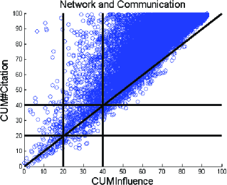
Figure 4: Comparison between Influence and Citation Count using cumulative value.

The two vertical and horizontal lines give the boundaries separating A and B from the rest of the ranks. Any author on the diagonal line received exactly the same ranking from both metrics. As we can see, there is correlation between Influence and CC - those with high CC ranking all have high Influence ranking as well. But the converse is not true - those with high Influence ranking may not have high CC ranking. This means we could use CC as a sufficient condition when estimating someone’s influence, but not a necessary condition. For this reason, we consider Influence is sufficiently different than CC, and should be considered as a complementary metric.

The Citation Value (CV) metric was designed to be an alternative to CC. From our experience, an author’s CV rank seems to be always between its CC rank and Influence rank. Fig. 5 compares CV against Influence.

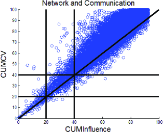
Figure 5: Comparison between Influence and Citation Value using cumulative value.

It is indeed similar to the comparison to CC, namely high CV implies high Influence but not vice versa. Thus, once we have CC and Influence, there is no strong reason to keep CV as an additional metric.

Now let us consider the Followers metric. As we observed in considering the Followers and Influence ranks for the Award recipients, those with a high influence rank tend to have even higher Followers ranks. But for the majority of the authors, these two ranks are very strongly correlated, and hence Followers seem to add little additional value to the Influence metric (as shown in Fig. 6).

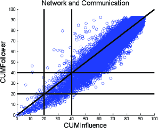
Figure 6: Comparison between Influence and Follower using cumulative value.

As expected, the Connections metric had little correlation to any of the other metrics. This is quite intuitive, so we have not included any similarity plots to save space.

Finally, we compared the Influence metric to the Exposure metric in Fig. 7.

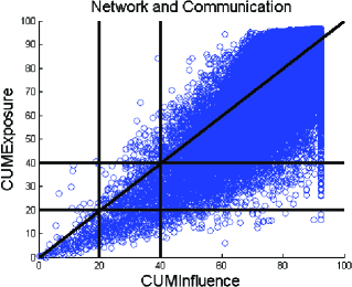
Figure 7: Comparison between Influence and Exposure using cumulative value.

In this case,many authors with low Influence values may have much higher ranks in Exposure. We suspect this is because this metric successfully identifies authors who are very active in publishing in high impact venues but have not had the time to build up their influence. It is difficult to tell how true this is - so we selected some real world examples for our case studies in a later subsection.

4.3 Similarity study with h-index

Next we investigated the similarity between the newly proposed metrics to the well known h-index Ball (2005); Hirsch (2005).

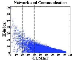
Figure 8: Comparison between cumulative Influence value and h-index.

We first compared the Influence metric to the h-index in Fig. 8. It is similar to the correlation between CC and Influence, i.e., those with high h-indices all have high Influence rankings as well. But the converse is not true - those with high Influence rankings may not have high h-indices. This reinforces the belief that influence is a better metric to differentiate those authors with high h-indices.

Next we compared the Exposure metric to the h-index in Fig. 9.

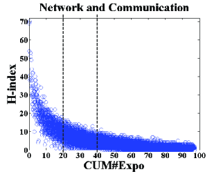
Figure 9: Comparison between cumulative Exposure value and h-index.

It shows again that high h-indices implies high Exposure rankings while the converse is not true. A clear difference that more points are located at the bottom left area, when comparing to Fig. 8. This is consistent with our suspicion that there exist many authors who are very active in publishing in high impact venues but their h-index values have not had enough time to accumulate. A similar argument was also raised by Harzing (2008).

At last, we looked into the total citation count versus the h-index of each author in Fig. 10.

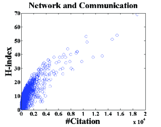
Figure 10: Comparison between total citation count and h-index.

As expected, the correlation between total citation counts and h-indices generally follows the square root law. This comes from the definition of the h-index Hirsch (2005).

4.4 Case Studies

From the above similarity study, we concluded that, out of the five metrics based on iterative computation, i.e. CV, Influence, Followers, Connections and Exposure, the first three are sufficiently similar: we therefore chose to keep only Influence. Influence, Connections and Exposure are sufficiently different from each other, and from CC.

For case studies, we considered two cases: (a) authors with high Influence but low Citation Count; and (b) authors with high Exposure but low Influence. (a) was the reason for keeping Influence, and (b) was the reason for keeping Exposure. We selected some such cases in the Network and Communications domain and show them in Table 10 and Table 11.

Table 10: Examples for High Influence and Low CC

Author	Influence	#Citation
Robert Elliot Kahn	A	C
J. M. Wozencraft	A	C
Jean-Jacques Werner	A	C
David G. Messerschmitt	A	C
Nathaniel S. Borenstein	A	C
James L. Massey	A	C
W. T. Webb	A	C
Takashi Fujio	A	D
Martin L. Shooman	A	D
Sedat Olcer	A	D
Massimo Marchiori	A	D
Roger A. Scantlebury	A	D

Table 11: Examples for High Exposure and Low Influence

Author	Influence	Exposure
Achille Pattavina	C	A
Herwig Bruneel	C	A
Yigal Bejerano	C	A
Torsten Braun	C	A
Kenneth J. Turner	C	A
Ioannis Stavrakakis	C	A
Emilio Leonardi	C	A
Luciano Lenzini	C	A
Dmitri Loguinov	C	A
Romano Fantacci	C	A
Hossam S. Hassanein	C	A
Azzedine Boukerche	C	A

4.5 Relation of Ranking to Publication Years

Finally, we were curious to find out the relationship between how an author ranked and his/her first (or last) year of publication. Fig. 11 plots the authors’ Influence ranks against their first year of publication.

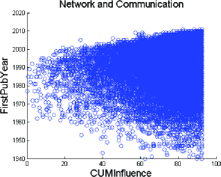
Figure 11: Comparison between Influence and the year of first publication.

It is worth noting that it takes time to build up Influence. Authors ranked as A in Influence started publishing in the 1990s or earlier; B authors started publishing in the early 2000s or earlier, and so on (here is the contribution based letter assignment).

Next, we plotted an author’s last year of publication against Influence (Fig. 12), Citation Count (Fig. 13), and then against h-index (Fig. 14), for comparison. Note, for Citation Count and h-index, the high ranking people are mostly still active, because we have been seeing paper and citation inflation over years. For Influence, however, there is more memory, in the sense that more people who are no longer active also enjoy high Influence. This is because an author’s influence propagates, by definition of the Influence metric.

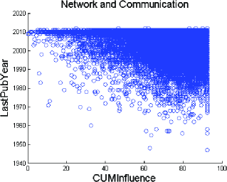
Figure 12: Comparison between Influence and the year of last publication.

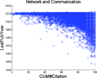
Figure 13: Comparison between Citation Count and the year of last publication.

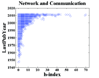
Figure 14: Comparison between h-index and the year of last publication.

4.6 Author-based Institution Rankings

In Table 12, we illustrate the possibility of institutional ranking according to authors’ rankings in various metrics. We selected 30 well-known universities and applied two counting granularities on authors’ letter grades of overall “Computer Science” rankings of three metrics, Citation Counts (CC), Influence (Inf) and Exposure (Exp).

Table 12: Illustration of Institution Rankings on 30 selected top universities of three metrics (#Citations, Influence and Exposure) at two counting granularities based on authors’ overall ranking in “Computer Science” domain.

Institution Name	Total Score Rank			#A Rank
	CC	Inf	Exp	CC	Inf	Exp
Massachusetts Institute of Technology	2	1	2	1	1	2
Carnegie Mellon University	1	2	1	2	2	1
Stanford University	3	3	3	4	4	4
University of California Berkeley	4	4	4	3	3	3
University of Illinois Urbana Champaign	5	5	5	6	6	5
University of Southern California	6	6	7	5	5	6
Georgia Institute of Technology	7	6	6	8	7	8
University of California San Diego	11	8	9	7	8	7
University of Washington	10	9	14	10	9	13
University of Maryland	8	9	8	9	11	8
University of California Los Angeles	12	11	11	12	10	12
University of Texas Austin	9	11	10	11	14	10
University of Michigan	13	13	11	14	14	16
Cornell University	15	14	15	13	11	15
University of Cambridge	16	15	21	17	17	22
Columbia University	17	16	19	21	20	17
University of Wisconsin Madison	20	17	28	18	18	22
University of Toronto	18	18	16	16	16	13
The French National Institute for	14	19	11	24	26	22
Research in Computer science and Control
University of Pennsylvania	22	20	27	21	21	22
Rutgers, The State University of New Jersey	23	21	22	29	18	22
Swiss Federal Institute of Technology Zurich	18	22	25	23	26	28
Harvard University	30	23	39	33	31	35
University of California Irvine	25	24	23	19	21	20
Purdue University	21	25	18	19	31	17
University of Minnesota	25	25	24	27	31	22
University of Massachusetts	24	25	26	31	36	30
Princeton University	27	28	29	14	13	17
Technion Israel Institute of Technology	31	29	19	24	23	10
University of Edinburgh	29	30	29	31	40	35

We found that the ranking results by different metrics were similar at the institution level. The noise at the author ranking results were cancelled out to a certain extent after they were aggregated for scores. When we used the two granularities: (1) count the number of authors assigned with “A” and (2) compute the total score, counting “A”=1, “B”=0.5, “C”=0.25 and “D”=“E”=0, for method (2), the size of an institution was influential; whereas for method (1), smaller schools also had a chance to rank very high. For example, in Table 12, Princeton University was ranked 28th by method (2), but 13th by only counting the number of “A” authors, i.e. by method (1).

Next we show three sets of similarity study between different institution ranking results, mainly focused on three selected metrics: Citation Count (CC), Influence (Inf) and Exposure (Exp). In the first set, we compared the ranking results at two different granularities, count number of “A” authors vs. compute total score, based on the rank percentile based letter grades, as shown in Fig. 15(b). In the second set (Fig. 16), we investigated how the authors’ letter grading methods (rank percentile based vs. contribution based) affect the total scores (granularity method (2)) as well as the institution rankings. In the last set, we compared three metrics (Inf vs. CC in Fig. 17(a), Inf vs. Exp in Fig. 17(b)) while the rank percentile based letter grading scheme and the granularity method (2) of computing total score are used.

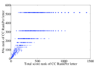
(a) CC

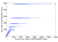
(b) Inf

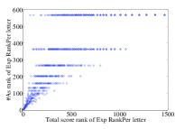
(c) Exp

Figure 15: Comparison on institution ranking results between two granularity methods: (counting number of As, y-axis) versus (counting “A”=1, “B”=0.5, “C”=0.25 for total score, x-axis) for three metrics, Citation Count (CC), Influence (inf) and Exposure (Exp) according to authors’ rank percentile based letter grades.

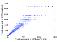
(a) CC

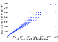
(b) Inf

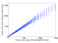
(c) Exp

Figure 16: Comparison on institution ranking results between rank percentile based (x-axis) versus contribution based (y-axis) letter grading methods, using granularity method (2) for three metrics, Citation Count (CC), Influence (inf) and Exposure (Exp).

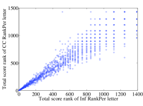
(a) Inf vs. CC

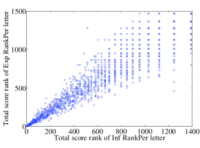
(b) Inf vs. Exp

Figure 17: Comparison on institution ranking results among three metrics, Citation Count (CC), Influence (inf) and Exposure (Exp) according to rank percentile based letter grading results using granularity method (2).

According to the above comparison results (Figures 15, 16 and 17), we made several observations:

1. As shown in Fig. 15, for those highly ranked institutions (e.g. above 100th), the ranking results of the two granularities are very close. In addition, as mentioned before, when the total scores (by counting “A”=1, “B”=0.5, “C”=0.25) were same, granularity method (1) can indicate the ratio of authors earning letter “A” (e.g. Princeton University in Table 12).
   

   On the other hand, counting the number of “A” authors only was ineffective in distinguishing institutions ranked below 100th (note the number of institutions with the same number of “A” authors located on horizontal lines).
   

2. As shown in Fig. 16, although the rank percentile based and contribution based letter grading methods make pronounced differences on author rankings, they produce very similar results on institution rankings.
   

3. As shown in Fig. 17, institutions ranked above 100th have similar ranking results for these three metrics (CC, Inf and Exp); however, the points are spread out largely for those ranked below 100th under different metrics. This again validates the effectiveness of the definitions of the various metrics with practical interpretations.

Finally, we compare our institution ranking approach to the three established ranking systems. We show the top 30 universities in “Computer Science” domain ranked by each of these systems, together with the ranking results by ours (based on total score of Influence metric):

1. US News Ranking - The Best Graduate Schools in Computer Science ranked in 2010 US-News (2010). Results are shown in Table 13.

2. The QS World University Rankings By Subject 2013 - Computer Science & Information Systems QS (2013). Results are shown in Table 14.

3. The Academic Ranking of World Universities (ARWU by SJTU) 2012 in Computer Science ARWU (2012). Results are shown in Table 15.

As in Tables 13-15, we find that the calculation of the overall score is the key factor leading to the deviation of the ranking results among different systems. In particular, the US New ranking system applied a subjective based approach US-News (2010) to calculate the total scores for each university. The QS ranking system calculated the overall score in the “Computer Science & Information Systems” subject based on the four objective factors: “Academic Reputation”, “Employer Reputation”, “Citations per Paper” and “H-index Citations” QS (2013). The ARWU ranking system, on the other hand, consider the overall score in “Computer Science” domain as the weighted average of the five metrics: “Alumni Turing Awards ($10\%$)”, “Staff Turing Award ($15\%$)”, “Highly Cited Researchers ($25\%$)”, “Papers indexed in SCI ($25\%$)” and “Papers Published in Top Journals ($25\%$)” ARWU (2012). Because of these factors (considering more reputation and recent work), the results of the three ranking systems tend to be quite volatile - the top universities change quite a bit from year to year. In our case of using total score of Influence metric, we are at least more stable and pure.

As Microsoft Libra also provides the institution ranking services Libra (2013), we make another comparison and the results are shown in Table 16. Since we are using the same dataset for calculation, it is not surprising that the ranking results are very similar.

Table 13: Top 30 Universities of “US News Ranking - The Best Graduate Schools in Computer Science ranked in 2010”, compared to ours (total score of Influence metric, Inf TS)

University Name	Score	USNews	Inf TS
Carnegie Mellon University	5.0	1	2
Massachusetts Institute of Technology	5.0	1	1
Stanford University	5.0	1	3
University of California Berkeley	5.0	1	4
Cornell University	4.6	5	14
University of Illinois Urbana Champaign	4.6	5	5
University of Washington	4.5	7	9
Princeton University	4.4	8	28
University of Texas Austin	4.4	8	11
Georgia Institute of Technology	4.3	10	6
California Institute of Technology	4.2	11	33
University of Wisconsin Madison	4.2	11	17
University of Michigan	4.1	13	13
University of California Los Angeles	4.0	14	11
University of California San Diego	4.0	14	8
University of Maryland	4.0	14	9
Columbia University	3.9	17	16
Harvard University	3.9	17	23
University of Pennsylvania	3.9	17	20
Brown University	3.7	20	42
Purdue University	3.7	20	25
Rice University	3.7	20	47
University of Massachusetts	3.7	20	25
University of North Carolina-Chapel Hill	3.7	20	42
University of Southern California	3.7	20	6
Yale University	3.7	20	53
Duke University	3.6	27	59
Johns Hopkins University	3.4	28	44
New York University	3.4	28	33
Ohio State University	3.4	28	40
Pennsylvania State University	3.4	28	46
Rutgers, The State University of New Jersey	3.4	28	21
University of California Irvine	3.4	28	24
University of Virginia	3.4	28	68

Table 14: Top 30 Universities of “The QS World University Rankings By Subject 2013 - Computer Science & Information Systems”, compared to ours (total score of Influence metric, Inf TS)

University Name	Score	QS	Inf TS
Massachusetts Institute of Technology	96.7	1	1
Stanford University	92.1	2	3
University of Oxford	92.0	3	21
Carnegie Mellon University	90.5	4	2
University of Cambridge	89.8	5	15
Harvard University	88.4	6	23
University of California Berkeley	88.0	7	4
National University of Singapore	87.2	8	57
Swiss Federal Institute of Technology Zurich	87.1	9	22
University of Hong Kong	84.0	10	165
Princeton University	83.7	11	28
The Hong Kong University of Science & Technology	83.6	12	113
The University of Melbourne	83.4	13	82
University of California Los Angeles	82.1	14	11
University of Edinburgh	81.5	15	30
University of Toronto	81.0	16	18
École Polytechnique Fédérale de Lausanne	80.2	17	36
Imperial College London	79.7	18	35
The Chinese University of Hong Kong	79.5	19	94
The University of Tokyo	79.4	20	50
Australian National University	78.9	21	107
Nanyang Technological University	78.5	22	91
University College London	78.0	23	47
The University of Sydney	77.9	24	146
The University of Queensland	77.8	25	107
Cornell University	77.6	26	14
Tsinghua University	77.5	27	107
University of Waterloo	77.5	27	32
The University of New South Wales	77.3	29	102
The University of Manchester	77.1	30	45

Table 15: Top 30 Universities of “The Academic Ranking of World Universities (ARWU by SJTU) 2012 in Computer Science, compared to ours (total score of Influence metric, Inf TS)

University Name	Score	SJTU	Inf TS
Stanford University	100	1	3
Massachusetts Institute of Technology	93.8	2	1
University of California Berkeley	85.3	3	4
Princeton University	78.7	4	28
Harvard University	77.7	5	23
Carnegie Mellon University	71.8	6	2
Cornell University	71.2	7	14
University of California Los Angeles	69.2	8	11
University of Texas Austin	68.3	9	11
University of Toronto	63.6	10	18
California Institute of Technology	63.5	11	33
Weizmann Institute of Science	63.3	12	89
University of Southern California	63.0	13	6
University of California San Diego	61.8	14	8
University of Illinois Urbana Champaign	61.7	15	5
University of Maryland	60.1	16	9
University of Michigan	58.9	17	13
Technion-Israel Institute of Technology	57.8	18	29
University of Oxford	56.7	19	31
Purdue University	54.5	20	25
University of Washington	54.2	21	9
Columbia University	53.8	22	16
Rutgers, The State University of New Jersey	53.5	23	21
Georgia Institute of Technology	53.0	24	6
Swiss Federal Institute of Technology Zurich	52.7	25	22
The Hong Kong University of Science & Technology	52.6	26	113
The Hebrew University of Jerusalem	52.5	27	77
Yale University	51.4	28	53
Tel Aviv University	50.9	29	36
The Chinese University of Hong Kong	50.7	30	94

Table 16: Top 30 Universities ranked by Libra in “Computer Science” domain, compared to ours (total score of Influence metric, Inf TS)

University Name	Field Rate	Libra	Inf TS
Stanford University	418	1	3
Massachusetts Institute of Technology	408	2	1
University of California Berkeley	404	3	4
Carnegie Mellon University	325	4	2
University of Illinois Urbana Champaign	268	5	5
Cornell University	260	6	14
University of Southern California	256	7	6
University of Washington	256	7	9
University of California San Diego	253	9	8
Princeton University	252	10	28
University of Texas Austin	248	11	11
University of California Los Angeles	243	12	11
University of Maryland	238	13	9
Georgia Institute of Technology	229	14	6
University of Michigan	224	15	13
University of Toronto	222	16	18
University of Cambridge	214	17	15
Harvard University	214	17	23
University of Wisconsin Madison	209	19	17
Columbia University	202	20	16
University of Pennsylvania	201	21	20
University of California Irvine	199	22	24
Rutgers, The State University of New Jersey	197	23	21
University of Oxford	197	23	31
University of Minnesota	195	25	25
Swiss Federal Institute of Technology Zurich	190	26	22
The French National Institute for	189	27	19
Research in Computer science and Control
California Institute of Technology	189	27	33
Brown University	189	27	42
University of Massachusetts	189	27	25

5 Related Works

The study of academic publication statistics is by no means a new topic. Previous attention focused mostly in different areas of science, especially physics. The most influential work was published in 1965 by Derek de Solla Price (1965), in which he considered papers and citations as a network and noticed the citation distribution (degree distribution) followed the power law. A few years later, he tried to explain this phenomenon using a simple model called the cumulative advantage process Derek de Solla Price (1976); Merton (1968). The skewness of the citation count distribution has since been validated by other studies on large scale datasets Seglen (1992); Redner (1998). In subsequent literature, later on, the model became better known as preferential attachment by Barabási and Albert (1999) (i.e. a paper is more likely to cite another paper with more existing citations) and with good empirical evidence Jeong et al (2003).

To determine the quality or impact of a paper by its citation count, while considered reasonable by many, has met with strong criticisms Walter et al (2003). Instead of using citation count, it has been proposed that a ranking factor, calculated using the eigenvector-based methods such as PageRank Brin and Page (1998) or HITS Kleinberg (1999), be adopted. Subsequently, a number of proposals of different variations to measure paper importance appeared, including eigenvector-based Sun and Giles (2007); Bergstrom (2007) or network traffic-like schemes Walker et al (2007); Li et al (2011). Since it takes time for a paper to accumulate its share of citations, it is common practice to use the venue (journal) the paper is published in to predict the potential impact/importance of a paper. Thus, Journal Impact Factor (JIF Garfield (1972)) becomes an important indicator used in practice.

The use of citation count has become more popular due to Google Scholar. More recently, some new indices, such as h-index Ball (2005); Hirsch (2005) and g-index Egghe (2006) have been proposed to combine the use of citation count and paper count to measure the achievements of an author. Some recent studies have also proposed to apply PageRank-type iterative algorithms to evaluate authors’ contribution and impact, notably a scheme called SARA (Scientific Author Ranking Algorithm) to compute authors contributions Radicchi et al (2009); and a model to rank both papers and authors Zhou et al (2007).

Besides the paper citations earned by authors, authors can also be ranked based on their connections and popularity as a co-author. This way of evaluating authors is used in a series of studies by Newman et al on author collaboration networks Newman (2001a, b, 2004a, 2004b). This approach and viewpoint is similar to that used in the study of social networks Easley and Kleinberg (2010). A number of recent papers studied social influence and their correlation to user actions Bakshy et al (2009); Anagnostopoulos et al (2008); Crandall et al (2008); Budalakoti and Bekkerman (2012).

Finally, the publication database plays a critical role in such bibliometrics and social network studies. The well-known databases are: Google Scholar, Scopus, ISI, CiteSeer Giles et al (1998), Microsoft Libra Libra (2013), DBLP Ley (2009), IEEE, ACM. These databases, however, tend to contain different papersets Chiu and Fu (2010). For example, CiteSeer, DBLP, ACM focus mostly on computer science and related literature, but each has its own rules of which conferences/papers to include or not. Not all these databases have citation information (e.g. DBLP does not).

6 Discussions

6.1 The name disambiguation problem

Name ambiguity is a big problem with online systems dealing with people names without explicit registration, especially true for bibliometric systems since the publication records come from many years of accumulation and from many different publishers. It is a hard problem, the full solution of which is beyond the scope of this paper. Below, we discuss some of the steps that have been taken and our plans for dealing with this problem in the future.

Our current implementation of the Academic Influence Ranking system makes full use of the objectized data from Microsoft Libra (2013). Each author is an object with its own ID. Microsoft Libra has already applied some name disambiguation algorithm to clean its raw data. We show two examples to illustrate this in Fig. 18.

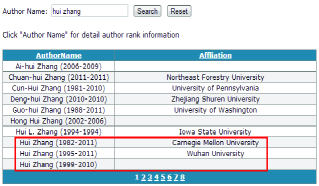
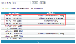
Figure 18: Examples of name disambiguation results.

As shown by the examples, multiple authors with the same name but different affiliations are included in Libra’s dataset, and we access the authors by their IDs.

From examining specific cases, we know that there still exist many author names (and their IDs) that are shared by many different real-world persons. MS Libra is also aware of this problem, evidenced by the fact that they submitted this problem as a challenge for the KDDCup (2013). We expect MS Libra will apply the algorithms proposed by the winning team of this competition in the near future. Since we plan to continue to update our system by sourcing data from MS Libra, we need to be careful in doing our own name disambiguation so that we can continue to leverage of the MS Libra data.

On the other hand, we are also using our tool and dataset for various statistical analysis, and model validation. For such purposes, it is sometimes adequate to disambiguate only the authors with significant publications. For this we can apply some semi-automatic and semi-manual methods. For example, we can automatically identify the author names worthy of disambiguation, and do the disambiguation semi-manually. Here are some semi-manual methods we are trying:

1. We have developed a crawler-parser to extract online information (e.g. author’s homepage) for given author names, and use that information to disambiguate authors with the same name.

2. We have also found certain online services with author registration, that can potentially help us disambiguate authors manually.
   

This allows us to be more confident with our statistical inferences.

In the long run, we believe the ultimate solution requires us to based everything on an (single) author registration system, so that all authors are guaranteed unique. This is clearly not a technical issue any more.

6.2 User feedbacks

We have demonstrated our system to many colleagues and friends, including some experts from the industry (Elsevier). Overall, we received very positive feedback. Here are some things people liked a lot:

1. By checking out the scores for authors familiar, the reviewers told us that the use of influence and connections seem to sort out the stronger researchers from those socially active researchers.

2. By checking the university ranking for domains familiar to them, the reviewers told us that the ranking is quite accurate, and the top universities are exactly the ones with strong groups in that domain.

3. Many told us that our website can be very useful for: (i) students searching for finding supervisors and graduate programs to apply; (ii) TPC chairs or journal editors finding people to review papers; (iii) hiring search; (iv) occasionally checking out someone to get their relative position roughly.

We also received many good suggestions that we will follow up in our future works. Here are some example ones:

1. It would be good to do controlled survey of (systematically selected) people in the different field, to see their opinions.

2. It would be good to introduce the concept of peer group for each person, and do comparison in that context. For example, a person’s peer group should include people of similar years of research experience.

3. It would be important to develop the user feedback component into the current website.

7 Conclusion

In this paper, we present the design and experimental study of an Academic Social Network website (http://pubstat.org) that we have built. It consists of several different non-conventional, social-network-like metrics we can use to rank authors and compare authors. In addition, it also provides author-based institution rankings by utilizing the author-institution relationship information. It has been demonstrated to many colleagues and friends, including some experts from industry (Elsevier). Overall, we received very positive feedback and many good suggestions that we will follow up in our future works.

Although we have had a working system for some time now, there are still many challenges to making it widely used. The publications database we have is not as complete as we would like; and we want to work out a way to continuously update it. The data is also far from clean. We are starting new projects to apply machine learning techniques to clean the data (some preliminary results in estimating missing years on papers have been submitted for publication).

We continue to discover new query types that users are interested in, and even new metrics. If the reviewers of this paper are interested in examining our website, we would be glad to open it for inspection in some fashion (http://pubstat.org).

Appendix A The PageRank Algorithm

Given a graph $G=(V,E)$, the PageRank Algorithm can be considered as a random walk starting from any node along the edges. After an infinite number of steps, the probability that a node is visited is the PageRank value of that node.

More formally, the probability distribution of visiting each node can be derived by solving a Markov Chain. The transition matrix $C$’s entries $c_{ij}$ ($i,j=1,2,\dots,n$) represent the transition probability that the random walk will visit node $j$ next given that it is currently at node $i$. Thus, $c_{ij}$ can be expressed as

$$c_{ij}=Prob(j|i)=\frac{e_{ij}}{\sum_{k}e_{ik}}$$ (1)

where $e_{ij}$ is from the adjacency matrix for the graph $G$. If $G$ is the citation graph, for example, then $e_{ij}=1$ if paper $i$ cites paper $j$; else $e_{ij}=0$.

In general, $C$ is a substochastic matrix with rows summing to either 0 (dangling nodes Brin and Page (1998), for example, representing papers with citing no other papers) or 1 (normal nodes, or papers). For each dangling node, the corresponding row is replaced by $\frac{1}{n}\mathbf{e}$, so that $C$ becomes a stochastic matrix.

In order to ensure the Markov Chain $C$ is irreducible, hence a solution is guaranteed to exist, $C$ is further transformed as follows:

$$\widetilde{C}=\alpha C+(1-\alpha)\mathbf{e}\mathbf{v}^{T},\;\;\alpha\in(0,1).$$ (2)

Here, $\mathbf{e}$ is a special column vector with all 1s, and of dimension $n$.

In Eq. (2), $\mathbf{v}\in\mathcal{R}^{n}$ is a probability vector (i.e. its values are between $0$ and $1$, and sum to $1$). It is referred to as the teleportation vector, which can be used to configure some bias into the random walk. For our purposes, we let $\mathbf{v}=1/n\mathbf{e}$ as the default setting.

Now, according to the Perron-Frobenius Theorem Langville and Meyer (2009); Meyer (2000), matrix $\widetilde{C}$ is stochastic, irreducible and aperiodic, and the equation

$$\mathbf{\pi}^{T}=\alpha\mathbf{\pi}^{T}C+(1-\alpha)\frac{1}{n}\mathbf{e}^{T},\;\;\alpha\in(0,1)$$ (3)

which can be solved by iteration methods in practice.

Appendix B Definition of Metrics in Matrix Form

We list the matrix form for the 5 metrics discussed in the previous sections in the following table:

Table 17: Notations and derivations of the ranking metrics.

Notations	Description
$n_{P}$	total number of papers
$n_{A}$	total number of authors
$n_{V}$	total number of venues
$(X)^{*}$	row normalization operation on any $X$, i.e.,
	$(X)_{ij}^{*}=\frac{X_{ij}}{\sum_{k}X_{ik}}$, for non-zero rows
$R$	$n_{P}\times n_{P}$ paper-citation adjacent matrix,
	$R_{ij}=1$, if paper $i$ has cited paper $j$
	0, otherwise.
$A$	$n_{P}\times n_{A}$ paper-author adjacent matrix,
	$A_{ij}=1$, if paper $i$ is written by author $j$
	0, otherwise.
$V$	$n_{P}\times n_{V}$ paper-venue adjacent matrix,
	$V_{ij}=1$, if paper $i$ has published in venue $j$
	0, otherwise.
$H$	$n_{A}\times n_{A}$ author influencing matrix,
	$H=(A^{T})^{*}(R)^{*}(A)^{*}$
$Y$	$n_{V}\times n_{V}$ venue influencing matrix,
	$Y=(V^{T})^{*}(R)^{*}(V)^{*}$
$F$	$n_{A}\times n_{A}$ author following indicating matrix,
	$F_{ij}=1$ if author $i$ has cited author $j$’s paper
	at least once, else 0.
$N$	$n_{A}\times n_{A}$ author collaboration matrix,
	$N=A^{T}A$
$T_{VA}$	$n_{V}\times n_{A}$ matrix, $T_{VA}=(V^{T})^{*}(A)^{*}$
$T_{AV}$	$n_{A}\times n_{V}$ matrix, $T_{AV}=(A^{T})^{*}(V)^{*}$
$P$	$(n_{A}+n_{V})\times(n_{A}+n_{V})$ matrix,
	$P=\left(\begin{array}[]{c c}\alpha(H)^{*}&(1-\alpha)T_{AV}\\ (1-\alpha)T_{VA}&\alpha(Y)^{*}\end{array}\right)$
Metrics	Description
CV	apply PageRank on $(R)^{*}$ to get papers CV,
	assign papers CV equally to authors,
	through, $\pi^{T}(A)^{*}$
Influence	apply PageRank on $(H)^{*}$
Follower	apply PageRank on $(F)^{*}$
Connection	apply PageRank on $(N)^{*}$
Exposure	apply PageRank on $P$, exposure of
	both authors and venues are obtained

References

- Anagnostopoulos et al (2008) Anagnostopoulos A, Kumar R, Mahdian M (2008) Influence and correlation in social networks. In: Proc. of the 14th ACM SIGKDD international conference on Knowledge discovery and data mining, pp 7–15
-
ARWU (2012)
ARWU (2012) The academic ranking of world universities (arwu by sjtu) 2012 in
computer science,
http://www.shanghairanking.com/SubjectCS2012.html - Bakshy et al (2009) Bakshy E, Karrer B, Adamic LA (2009) Social influence and the diffusion of user-created content. In: Proc. of the 10th ACM Conference on Electronic Commerce (EC), pp 325–334
- Ball (2005) Ball P (2005) Index aims for fair ranking of scientists. Nature 436:900
- Barabási and Albert (1999) Barabási AL, Albert R (1999) Emergence of scaling in random networks. Science 286:509–512
- Bergstrom (2007) Bergstrom C (2007) Eigenfactor: Measuring the value and prestige of scholarly journals. Coll Res 68(5)
- Brin and Page (1998) Brin S, Page L (1998) The anatomy of a large-scale hypertextual web search engine. In: Proc. of the 7th international conference on Would Wide Web (WWW)
- Budalakoti and Bekkerman (2012) Budalakoti S, Bekkerman R (2012) Bimodal invitation-navigation fair bets model for authority identification in a social network. In: Proceedings of the 21st international conference on World Wide Web, ACM, pp 709–718
- Chiu and Fu (2010) Chiu DM, Fu TZJ (2010) “Publish or Perish” in the Internet Age: a study of publication statistics in computer networking research. ACM Sigcomm Computer Communication Review (CCR) 40(1):34–43
- Crandall et al (2008) Crandall D, Cosley D, Huttenlocher D, Kleinberg J, Suri S (2008) Feedback effects between similarity and social influence in online communities. In: Proc. of the 14th ACM SIGKDD international conference on Knowledge discovery and data mining, pp 160–168
- Easley and Kleinberg (2010) Easley DA, Kleinberg JM (2010) Networks, Crowds, and Markets - Reasoning About a Highly Connected World. Cambridge University Press
- Egghe (2006) Egghe L (2006) An improvement of the h-index: The g-index. ISSI Newsletter 2(1):8–9
- Garfield (1972) Garfield E (1972) Citation analysis as a tool in journal evaluation. Science 178(60):471–479
- Giles et al (1998) Giles CL, Bollacker KD, Lawrence S (1998) Citeseer: An automatic citation indexing system. In: Proceedings of the third ACM conference on Digital libraries, pp 89–98
-
Harzing (2008)
Harzing AW (2008) Reflections on the h-index,
http://www.harzing.com/pop_hindex.htm/ - Hirsch (2005) Hirsch JE (2005) An index to quantify an individual’s scientific research output. Proceedings of the National Academy of Sciences of the United States of America 102:16,569–16,572
- Jeong et al (2003) Jeong H, Néda Z, Barabási AL (2003) Measuring preferential attachment in evolving networks. Europhys Lett 61:567–572
-
KDDCup (2013)
KDDCup (2013) Author disambiguation challenge,
http://www.kaggle.com/c/kdd-cup-2013-author-disambiguation/ - Kleinberg (1999) Kleinberg JM (1999) Authoritative sources in a hyperlinked environment. Journal of ACM 48:604–632
- Langville and Meyer (2009) Langville AN, Meyer CD (2009) Google’s PageRank and Beyond: The Science of Search Engine Rankings. Princeton University Press
- Ley (2009) Ley M (2009) Dblp: some lessons learned. Proceedings of the VLDB Endowment 2(2):1493–1500
- Li et al (2011) Li P, Yu JX, Liu H, nd Xiaoyong Du JH (2011) Ranking individuals and groups by influence propagation. In: Proc. of PAKDD(2), pp 407–419
-
Libra (2013)
Libra (2013) Microsoft academic search,
http://academic.research.microsoft.com/ - Merton (1968) Merton RK (1968) The matthew effect in science. Science 159:56–63
- Meyer (2000) Meyer CD (2000) Matrix analysis and applied linear algebra. SIAM Philadelphia
- Newman (2001a) Newman MEJ (2001a) Clustering and preferential attachment in growing networks. Phys Rev E 64:025,102
- Newman (2001b) Newman MEJ (2001b) The structure of scientific collaboration networks. Proc Natl Acad Sci USA 98(2):404–409
- Newman (2004a) Newman MEJ (2004a) Coauthorship networks and patterns of scientific collaboration. Proc Natl Acad Sci USA 101:5200–5205
- Newman (2004b) Newman MEJ (2004b) Who is the best connected scientist? a study of scientific coauthorship networks. Springer pp 337–370
- Nie et al (2007) Nie Z, Wen J, Ma W (2007) Object-level vertical search. In: Proceedings of the 3rd Biennial Conference on Innovative Data Systems Research (CIDR)
- QS (2013) QS (2013) The QS world university rankings by subject 2013 - computer science & information systems, http://www.topuniversities.com/university-rankings/university-subject-rankings/2013/computer-science-and-information-systems/
- Radicchi et al (2009) Radicchi F, Fortunato S, Markines B, Vespignani A (2009) Diffusion of scientific credits and the ranking of scientists. Physical Review E 80:056,103
- Redner (1998) Redner S (1998) How popular is your paper? an empirical study of the citation distribution. Eur Phys J B 4:131–134
- Seglen (1992) Seglen PO (1992) The skewness of science. J Amer ScoInform Sci 43:628–638
- de Solla Price (1965) de Solla Price DJ (1965) Networks of scientific papers. Science 149(3683):510–515
- de Solla Price (1976) de Solla Price DJ (1976) A general theory of bibliometric and other cumulative advantage process. J Amer Soc Inform Sci 27:292–306
- Sun and Giles (2007) Sun Y, Giles CL (2007) Popularity weighted ranking for academic digital libraries. In: Proc. of the 29th European Conference on Information Retrieval Research (ECIR 2007)
- US-News (2010) US-News (2010) US News Ranking - the best graduate schools in computer science, http://grad-schools.usnews.rankingsandreviews.com/best-graduate-schools/top-science-schools/computer-science-rankings/
- Walker et al (2007) Walker D, Xie H, Yan KK, Maslov S (2007) Ranking scientific publications using a model of network traffic. Journal of Statistical Mechanics p p06010
- Walter et al (2003) Walter G, Bloch S, Hunt G, Fisher K (2003) Counting on citations: a flawed way to measure quality? Medical Journal of Australia 178:280–1
- Zhou et al (2007) Zhou D, Orshanskiy SA, Zha H, Giles CL (2007) Co-ranking authors and documents in a heterogeneous network. In: Proc. of IEEE International Conference on Data Mining (ICDM)