Enhancement of critical temperatures in disordered bipartite lattices

Abstract

We study the strong enhancement, induced by random hopping, of the critical temperatures characterizing the transitions to superconductivity, charge-density wave and antiferromagnetism, which can occur in bipartite lattice models at half-filling, like graphene, by means of an extended Finkel’stein non-linear $\sigma$-model renormalization group approach. We show that, if Cooper channel interaction dominates, superconducting critical temperature can be enhanced at will, since superconductivity cannot be broken by entering any Anderson insulating phase. If instead, staggered interactions are relevant, antiferromagnetic order is generated by disorder at a temperature well above that expected for a clean system.

I Introduction

The interplay of disorder and interactions is the origin of several interesting and still unclear phenomena in condensed matter physics. One interesting problem raised in the past concerned the influence of randomness on Bardeen-Cooper-Schrieffer superconductors. It is well known that, in the absence of interaction, disorder can induce an insulating behavior on the electron systems, the so-called Anderson insulator anderson . On the other hand, an attractive interaction makes the system unstable towards superconductivity. It was shown that a weak disorder does not spoil superconductivity anderson2 and the critical temperature $T_{c}$ is essentially unaffected by impurities lee ; kapit . However, in the presence of long-range Coulomb repulsion, diffusion of charges can lead to a suppression of superconducting $T_{c}$ fukuyama ; finkelstein . Quite recently, instead, it was shown that $T_{c}$ can even be increased by Anderson localization kravtsov ; kravtsov2 ; burmistrov , provided that Coulomb interaction is screened and sufficiently weak.

There are, however, disordered systems which do not show an Anderson insulating behavior, being close to the so-called Gade-Wegner criticality gade . They are known as two-sublattice models, possessing a special symmetry called sublattice symmetry (namely, when only sites belonging to different sublattices are coupled), which usually describe particles randomly hopping (without on-site disorder) in nearest-neighbor sites on half-filled bipartite lattices, such as the square lattice or the honeycomb lattice, as in the case of graphene, which is naturally at half filling. Indeed when the impurity potential is close to the unitary scattering limit pepin (when the impurity potential is infinitely strong) it reduces, by taking out one site, to a random nearest-neighbor hopping. This is what experimentally can be realized with graphene by substitutional doping or by vacancies. The conductivity, with random hopping and in the absence of interactions, does not acquire any quantum interference corrections which would lead to Anderson localization, in contrast to systems with on-site disorder. The role of interactions in such systems, which are not Anderson insulators, is the missing piece of the puzzle.

The important issue we will address in this paper is related to the question whether Cooper pair instability can be promoted by disorder in such systems and if disorder can unexpectedly improve a charge-density wave or generate a magnetic order.
We actually find that random hopping strongly enhances all the critical temperatures allowed in these systems, with respect to those obtained in the clean case, which delimit the transitions from normal phase to (i) superconductivity (SC), if the particle-particle Cooper channel dominates in the electron-electron interaction; (ii) charge-density wave (CDW), if, instead, a staggered particle-hole singlet channel is dominant; and, finally, (iii) antiferromagnet (AFM), if a staggered particle-hole triplet channel prevails. The main advantage of such random hopping two-sublattice systems as compared to standard systems (where sublattice symmetry is broken, for instance, by on-site disorder) is that one can improve almost ad libitum the transition temperatures, such as the superconducting critical temperature, by increasing the disorder parameters and tuning the residual interactions, never entering the Anderson insulating phase, which would break superconductivity. In addition, other instabilities (AFM, CDW) are allowed, which are not present in the standard case.

To study the role of randomness in electron systems, one can resort to a quantum field theory approach for disordered systems wegner ; efetov , further improved to deal with combined effects of interactions and disorder. finkelstein ; castellani ; belitz The interaction parameters acquire a scale dependence and, together with the conductance, form a full set of couplings of the so-called Finkel’stein non-linear $\sigma$ model, which flow under the action of the renormalization group (RG). Since we are interested in Cooper pair formations we will focus our attention to the systems in which time-reversal symmetry is preserved. The Wigner-Dyson class of symmetry covered by the standard Finkel’stein model is then the AI class (with time reversal and spin-rotation invariance, without sublattice symmetry). zirnbauer ; mirlin ; note The symmetry class we are going to consider in this paper is the so-called BDI class, by the inclusion of the sublattice symmetry which produces anomalous behaviors already in the non-interacting case gade ; michele . One has, therefore, to extend the Finkel’stein model npb ; ludwig in the way shown in Appendix.

II RG equations for BDI class

Considering, therefore, the case where both sublattice symmetry and time-reversal symmetry are preserved (BDI class), the complete one-loop RG equations at $d=2+\epsilon$ dimensions, are given by Eqs. (1)-(II). Since the dephasing scattering rate for our interacting particles is basically given by the temperature $T$, the integration of the RG equations will run from $T$ to some energy cutoff $\omega_{o}$, which, for our purposes, can be fixed by the Debye energy. The scaling parameter is, therefore, given by $\ell=\ln(\omega_{o}/T)$. For convenience we rescale $T\rightarrow\omega_{o}T$ so that the diffusive regime we are going to consider is defined for $T\leq 1$, i.e. for $\ell=\ln(1/T)\geq 0$. Our bare starting parameters are taken at $T=1$, (at $\ell=0$), namely, at the scale corresponding to $\omega_{o}$. The equations are (see Ref. npb for more details)

$$\frac{dg}{d\ell} = -\epsilon g+{g^{2}}\left\{6+\frac{1-\gamma_{s}^{0}}{\gamma_{s}^{0}}\,\ln(1-\gamma_{s}^{0})-\frac{1}{2}\gamma_{s}^{3}-3\,\frac{1+\gamma_{t}^{0}}{\gamma_{t}^{0}}\,\ln(1+\gamma_{t}^{0})+\frac{3}{2}\gamma_{t}^{3}-\gamma_{c}^{0}+2\,\frac{1-\gamma_{c}^{3}}{\gamma_{c}^{3}}\,\ln(1-\gamma_{c}^{3})\right\}$$ (1)

$$\frac{d\Gamma}{d\ell} = \epsilon\Gamma+8g+\frac{\Gamma}{g}\frac{dg}{d\ell}$$ (2)

$$\frac{d\gamma^{0}_{t}}{d\ell} = g\left\{\left(1+\gamma_{t}^{0}\right)\left(-\frac{3}{2}-\frac{\Gamma}{8}+\frac{\gamma_{s}^{0}}{2}-\frac{\gamma_{s}^{3}}{2}-\gamma_{c}^{0}+\gamma_{c}^{3}+\frac{3}{2}\gamma_{t}^{3}\right)+\left(1+\gamma_{t}^{0}\right)^{2}\left(\frac{3}{2}+\frac{\Gamma}{8}+\gamma_{s}^{3}-\gamma_{t}^{3}\Big{(}1-\frac{\Gamma}{4}\Big{)}+2\gamma_{c}^{0}\right)-2(\gamma_{t}^{3})^{2}\right\}$$ (3)

$$\frac{d\gamma^{3}_{t}}{d\ell} = g\left\{\left(\frac{1}{2}+\frac{\Gamma}{4}\right)\gamma_{t}^{0}+\left(\frac{3}{2}+\frac{\Gamma}{8}+\ln\left[\frac{(1-\gamma_{c}^{3})^{2}(1-\gamma_{s}^{{}^{0}})}{1+\gamma_{t}^{0}}\right]\right)\gamma_{t}^{3}+\frac{\gamma_{s}^{3}}{2}+\frac{\gamma_{s}^{0}}{2}+\gamma_{c}^{0}+\gamma_{c}^{3}\right.$$

$$+\gamma_{t}^{3}\left(\frac{1}{2}\gamma_{s}^{0}-\frac{3}{2}\gamma_{t}^{0}+\gamma_{c}^{3}\left.+\gamma_{c}^{0}-\frac{3}{2}\gamma_{t}^{3}+\frac{1}{2}\gamma_{s}^{3}\right)\right\}+(\gamma_{t}^{3})^{2}$$

$$\frac{d\gamma^{0}_{s}}{d\ell} = g\left\{\left(1-\gamma_{s}^{0}\right)\left(\frac{1}{2}+\frac{\Gamma}{8}+\frac{\gamma_{s}^{3}}{2}+\gamma_{c}^{0}-\gamma_{c}^{3}+\frac{3}{2}(\gamma_{t}^{0}-\gamma_{t}^{3})\right)-\left(1-\gamma_{s}^{0}\right)^{2}\left(\frac{1}{2}+\frac{\Gamma}{8}+\gamma_{s}^{3}\Big{(}1-\frac{\Gamma}{4}\Big{)}-\frac{2\gamma_{c}^{3}}{1-\gamma_{c}^{3}}-3\gamma_{t}^{3}\right)+2(\gamma_{c}^{0})^{2}\right\}\phantom{,}$$ (5)

$$\frac{d\gamma^{3}_{s}}{d\ell} = g\left\{\frac{3}{2}\gamma_{t}^{0}+\frac{3}{2}\gamma_{t}^{3}+\left(\frac{1}{2}+\frac{\Gamma}{8}+\ln\left[(1+\gamma_{t}^{0})^{3}(1-\gamma_{s}^{0})(1-\gamma_{c}^{3})^{2}\right]\right)\gamma_{s}^{3}-\left(\frac{1}{2}-\frac{\Gamma}{4}\right)\gamma_{s}^{0}+\gamma_{c}^{3}\right.$$

$$+\gamma_{c}^{0}\left(1-4\ln(1-\gamma_{c}^{3})\right)+\gamma_{s}^{3}\left(\frac{1}{2}\gamma_{s}^{0}-\frac{3}{2}\gamma_{t}^{0}+\gamma_{c}^{3}\left.-\frac{3}{2}\gamma_{t}^{3}+\frac{1}{2}\gamma_{s}^{3}+\gamma_{c}^{0}\right)\right\}-(\gamma_{s}^{3})^{2}\phantom{--}$$

$$\frac{d\gamma^{0}_{c}}{d\ell} = g\left\{\frac{3}{2}\gamma_{t}^{0}+\frac{3}{2}\gamma_{t}^{3}+\frac{\gamma_{s}^{0}}{2}+\frac{\gamma_{s}^{3}}{2}+\left(1+\frac{\Gamma}{8}+\ln\left[\frac{(1+\gamma_{t}^{0})^{3}(1-\gamma_{c}^{3})^{2}}{(1-\gamma_{s}^{0})}\right]\right)\gamma_{c}^{0}+\frac{\Gamma}{4}\gamma_{c}^{3}\right.$$

$$-2\gamma_{s}^{3}\ln(1-\gamma_{c}^{3})+\gamma_{c}^{0}\left(\frac{1}{2}\gamma_{s}^{0}-\frac{3}{2}\gamma_{t}^{0}+\gamma_{c}^{3}\left.-\frac{3}{2}\gamma_{t}^{3}+\frac{1}{2}\gamma_{s}^{3}+\gamma_{c}^{0}\right)\right\}-(\gamma_{c}^{0})^{2}$$

$$\frac{d\gamma^{3}_{c}}{d\ell} = g\left\{-1-\gamma_{c}^{0}+\gamma_{s}^{0}+\gamma_{s}^{3}-2\gamma_{c}^{3}\left(\ln(1-\gamma_{c}^{3})-\frac{\gamma_{c}^{3}}{\gamma_{s}^{0}}\ln(1-\gamma_{s}^{0})\right)+2\gamma_{c}^{0}\gamma_{s}^{3}\right.$$

$$+\left(1-\gamma_{c}^{3}\right)\left(3+\frac{\Gamma}{8}+3\gamma_{c}^{0}-\frac{\gamma_{s}^{0}}{2}-\frac{3}{2}\gamma_{s}^{3}+\frac{3}{2}\left(\gamma_{t}^{0}-\gamma_{t}^{3}\right)\right)\left.+\left(1-\gamma_{c}^{3}\right)^{2}\left(-2-\frac{\Gamma}{8}-2\gamma_{c}^{0}+\frac{\Gamma}{4}\gamma_{c}^{0}+\gamma_{s}^{3}+3\gamma_{t}^{3}\right)\right\}$$

In Eqs. (1-II) the disorder parameters are: $g$, the charge resistivity, and $\Gamma$, related to the non-zero mean bond dimerization of the original lattice gade ; michele ; npb ; ludwig . Notice that, for $\epsilon=0$ and in the limit of all $\gamma\rightarrow 0$, Eq. (1) becomes $dg/d\ell=0$, namely, $g$ remains constant. This non-interacting behavior is what is called the Gade-Wegner criticality gade ; mirlin . The interaction parameters are related to (i) smooth interactions: $\gamma_{s}^{0}$ (particle-hole singlet channel), $\gamma_{t}^{0}$ (particle-hole triplet channel), $\gamma_{c}^{0}$ (particle-particle Cooper channel); and (ii) staggered sublattice interactions: $\gamma_{s}^{3}$ (particle-hole singlet), $\gamma_{t}^{3}$ (particle-hole triplet), and $\gamma_{c}^{3}$ (particle-particle). Among these parameters, $\gamma_{t}^{3}$, $\gamma_{s}^{3}$ and $\gamma_{c}^{0}$ are responsible for antiferromagnetic spin density wave (AFM), charge density wave (CDW) and $s$-wave superconductivity (SC), respectively. The very last terms in Eqs. (II), (II, and (II), those not coupled to $g$, are actually, the terms which can drive the system to AFM ($\gamma_{t}^{3}$), CDW ($\gamma_{s}^{3}$), and SC ($\gamma_{c}^{0}$) also in clean systems, obtained by simple ladder summations. Equations (1)-(II) are quite complicated; nevertheless, they hide an amazing property: they, in fact, are symmetric under the transformation $\gamma_{s}^{0}=\gamma_{c}^{3}\leftrightarrow-\gamma^{0}_{t}$ and $\gamma_{s}^{3}=\gamma_{c}^{0}\leftrightarrow-\gamma^{3}_{t}$. This symmetry property of the parameters can be obtained by particle-hole transformation of the original fermionic fields defined on the lattice, $c_{i\uparrow}\rightarrow c_{i\uparrow}$, $c_{i\downarrow}\rightarrow(-)^{i}c^{\dagger}_{i\downarrow}$, which maps charge to spin and vice versa. By imposing $\gamma^{0}_{s}=\gamma_{c}^{3}=-\gamma_{t}^{0}\equiv\gamma$, and $\gamma^{3}_{s}=\gamma_{c}^{0}=-\gamma_{t}^{3}\equiv\bar{\gamma}$, namely, considering the peculiar particle-hole symmetric case, Eqs. (1)-(II) are strongly simplified (see Appendix) These conditions, actually, define a subspace of the full space of parameters, invariant under RG flow.

III Analytical solutions

For starting amplitudes fulfilling $|\gamma_{c}^{0}|\gg|\gamma_{s}^{0}|,|\gamma_{t}^{0}|,|\gamma_{c}^{3}|,|\gamma_{t}^{3}|,|\gamma_{s}^{3}|$, Eqs. (1)-(II) can be approximated as follows: $dg/d\ell\simeq-\epsilon g$, $d\Gamma/d\ell\simeq 8g$, $d\gamma_{s}^{0}/d\ell\simeq d\gamma_{t}^{0}/d\ell\simeq d\gamma_{s}^{3}/d\ell\simeq d\gamma_{t}^{3}/d\ell\simeq g\gamma_{c}^{0}$, $d\gamma_{c}^{3}/d\ell\simeq\Gamma g\gamma_{c}^{0}/4$, and finally

$$\frac{d\gamma_{c}^{0}}{d\ell}\simeq\eta\,\gamma_{c}^{0}-(\gamma_{c}^{0})^{2}\,,$$ (9)

where $\eta\equiv z-d=g\left(1+\frac{\Gamma}{8}\right)$, with $z$ being the dynamical exponent. The solution of Eq. (9), for $\epsilon=0$, is

$$\gamma_{c}^{0}(\ell)\simeq\frac{\gamma_{c}^{0}\,e^{\frac{\eta(\ell)^{2}}{2g_{0}^{2}}}}{e^{\frac{\eta_{0}^{2}}{2g_{0}^{2}}}+\frac{\gamma_{c}^{0}}{g_{0}}\sqrt{\frac{\pi}{2}}\left(\textrm{erfi}\left(\frac{\eta(\ell)}{\sqrt{2}g_{0}}\right)-\textrm{erfi}\left(\frac{\eta_{0}}{\sqrt{2}g_{0}}\right)\right)}$$ (10)

where $\gamma_{c}^{0}$ here means $\gamma_{c}^{0}(0)$, to make notation simpler, $\textrm{erfi}(y)=\frac{2}{\sqrt{\pi}}\int_{0}^{y}e^{x^{2}}dx$ is the imaginary error function and $\eta(\ell)\simeq\eta_{0}+g_{0}^{2}\ell$, with $g_{0}=g(0)$ and $\eta_{0}=g_{0}(1+\frac{\Gamma_{0}}{8})$.
For $\gamma_{c}^{0}<0$ the system is unstable towards superconductivity whose $T_{c}$, for $\eta_{0}\ll|\gamma_{c}^{0}|$, at leading orders, is

$$T_{c}\sim\exp\left(-\frac{1}{|\gamma_{c}^{0}|}\left(1-\frac{\eta_{0}}{2|\gamma_{c}^{0}|}\right)\right).$$ (11)

One can see that, for $g_{0}\rightarrow 0$, namely for a clean system, one recovers the known result $T_{c}=T_{c}^{BCS}\sim e^{-{1}/{|\gamma_{c}^{0}|}}$. In other words, the disorder parameter $\eta_{0}$, which is always positive, improves $T_{c}$. The enhancement is stronger for large disorder. For $\eta_{0}\sim g_{0}\gg|\gamma_{c}^{0}|$, in fact, we get

$$T_{c}\sim\exp\left(-\frac{{\cal C}}{g_{0}}\right)\,,$$ (12)

where ${\cal C}={\cal C}(g_{0},\gamma_{c}^{0})\approx\sqrt{W\left((g_{0}/|\gamma_{c}^{0}|)^{2}\right)}$, a smooth function ($W(x)$ is the Lambert function or product logarithm).

In the special particle-hole symmetric case, for $g_{0}\ll|\bar{\gamma}|$ and $\Gamma_{0}\simeq 0$, $\ln T_{c}$ increases quadratically with $g_{0}$ (see Appendix) instead of linearly as in Eq. (11). This deviation from linearity is observed already when $|\gamma_{s}^{3}|$ and $|\gamma_{t}^{3}|$ become of the same order of $|\gamma_{c}^{0}|$, as shown in Fig. 1, for small $g_{0}$.

Before concluding this section, a couple of comments is in order. As declared also in Ref. burmistrov , strictly in 2D the SC transition is of the Berezinskii-Kosterliz-Thouless (BKT) type, whereas we have calculated the mean-field transition temperature (which identifies Cooper pairs formation). However, since the mean-field and BKT temperatures do not differ much beasley , we expect that the enhancement of $T_{c}$ holds also for $T_{BKT}$. Finally, for very strong disorder ($g\,\Gamma\gg 1$) we would expect that the dynamical exponent is affected by a sort of electron freezing effect motrunich ; mudry ; npb1 , a weak multifractal effect which modifies $z$ as $z\sim\sqrt{g\,\Gamma}$. As a result, in the strong disorder regime, Eq. (12) should turn into $T_{c}\sim\exp\left(-{\tilde{\cal C}}/{g^{{2}/{3}}}\right)$.

For $\epsilon>0$, since $\frac{d\eta}{d\ell}=-\epsilon\eta+O(g^{2})$, Eq. (9), can be rewritten as $\frac{d\gamma_{c}^{0}}{d\eta}\simeq-\frac{\gamma_{c}^{0}}{\epsilon}+\frac{(\gamma_{c}^{0})^{2}}{\epsilon\eta}$ whose solution, for $\eta_{0}\ll\epsilon$, gives the following critical temperature

$$T_{c}\sim\left(T_{c}^{BCS}\right)^{1-({\eta_{0}}/{\epsilon})}.$$ (13)

$T_{c}$ is still enhanced by disorder with respect to $T_{c}^{BCS}$. Notice that the disorder parameter, $\eta_{0}\sim g_{0}$, can be arbitrarily strong, compared to $|\gamma_{c}^{0}|$, and that $T_{c}$ and $T_{c}^{BCS}$ $<1$, being both rescaled by the energy cutoff $\omega_{o}$.

Analogously, one can study the instabilities towards spin or charge density waves when only $\gamma_{t}^{3}$ or $\gamma_{s}^{3}$ dominate, finding similar expressions for the corresponding critical temperatures. In particular for $|\gamma_{s}^{3}|$ greater than all the other parameters, we have to solve

$$\frac{d\gamma_{s}^{3}}{d\ell}\simeq\left(\eta-\frac{g}{2}\right)\,\gamma_{s}^{3}-(\gamma_{s}^{3})^{2}$$ (14)

whose solution, for $\gamma_{s}^{3}<0$, gives a critical temperature for CDW with the same behaviors as in Eqs. (11)-(13) with $\gamma_{c}^{0}$ replaced by $\gamma_{s}^{3}$, $\eta_{0}$ by $(\eta_{0}-g_{0}/2)$, and $T_{c}^{BCS}$ by $\exp{(-1/|\gamma_{s}^{3}|)}$. For $|\gamma_{t}^{3}|$ dominant, instead, we have

$$\frac{d\gamma_{t}^{3}}{d\ell}\simeq\left(\eta+\frac{g}{2}\right)\,\gamma_{t}^{3}+(\gamma_{t}^{3})^{2}$$ (15)

which, for $\gamma_{t}^{3}>0$, drives the system to AFM with a new Néel temperature given by Eqs. (11)-(13), where $\gamma_{c}^{0}$ is replaced by $\gamma_{t}^{3}$, $\eta_{0}$ by $(\eta_{0}+g_{0}/2)$, and $T_{c}^{BCS}$ by the Néel temperature $\exp{(-1/\gamma_{t}^{3})}$ of the clean system.

IV RG solutions

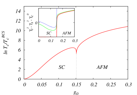
Figure 1: (Color online) Critical temperature, in log-scale, in units of $T_{c}^{BCS}$ as a function of the initial value for $g$ ($g_{0}\equiv g(\ell=0)$), obtained for the following starting parameters: $\epsilon=0$, $\Gamma(\ell=0)=0$, $\gamma_{s}^{0}(0)=\gamma_{t}^{0}(0)=\gamma_{c}^{3}(0)=0.01$, $\gamma_{c}^{0}(0)=-0.065$, $\gamma_{s}^{3}(0)=-0.04$, $\gamma_{t}^{3}(0)=0.04$. For $g_{0}<0.15$, $T_{c}$ is the superconducting critical temperature (SC) while for $g_{0}>0.15$, $T_{c}$ is the Néel temperature for antiferromagnets (AFM). The vertical dotted line only projects $T_{c}$ where the two instabilities exchange. Inset: the parameters, $\gamma_{s}^{3}$ (green long dashed line), $\gamma_{t}^{3}$ (blue dashed line), $\gamma_{c}^{0}$ (red solid line), at $T=T_{c}$, as functions of $g_{0}$.

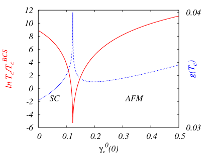
Figure 2: (Color online) Critical temperature (red-solid line), in log-scale, in units of $T_{c}^{BCS}$ as a function of the initial value for the particle-hole singlet interaction $\gamma_{s}^{0}(\ell=0)$, at $\epsilon=0$, obtained for the following initial parameters: $g_{0}=0.03$, $\Gamma(0)=0$, $\gamma_{t}^{0}(0)=-\gamma_{c}^{3}(0)=0.001$, $\gamma_{c}^{0}(0)=-0.04$, $\gamma_{t}^{3}(0)=-\gamma_{s}^{3}(0)=0.001$. For $\gamma_{s}^{0}(0)<0.12245$, $T_{c}$ is the SC critical temperature, otherwise it is the critical temperature for AFM. For the same initial conditions, the renormalized $g$, when $T=T_{c}$, is plotted (blue-dashed line) as a function of $\gamma_{s}^{0}(0)$.

A richer variety of behaviors can be found by solving the full set of Eqs. (1)-(II) (by using the FORTRAN code provided in Ref. supplement ). It can happen that small and large disorder regimes can be characterized by different phases. In particular, we found that AFM is the most favoured instability, provided that $\gamma_{t}^{3}>0$. If $\gamma_{c}^{0}$ is the dominant parameter but $\gamma_{t}^{3}$ is also sizable, by increasing disorder ($g_{0}$) the superconducting $T_{c}$ is enhanced up to a value of $g_{0}$ above which AFM may prevail, whose corresponding critical temperature is much higher than the Néel temperature in a clean system, i.e. $T_{c}\gg\exp(-1/\gamma_{t}^{3})$ (see Fig. 1). An important role in the occurrence of AFM is played also by the other parameters, even when they start with small values. It is crucial, therefore, to take into account all the contributions appearing in Eqs. (1-II), in order to draw correctly the boundaries of different phases. By fixing the disorder strength $g_{0}$ but increasing the bare parameter $\gamma_{s}^{0}(0)$, the SC $T_{c}$ is suppressed. For sufficiently large $\gamma_{s}^{0}$, then the dominant instability turns to be the AFM again (see Fig. 2). In other words, we can go from an $s$-wave superconducting regime to a magnetic ordered regime, not only by simply increasing the triplet staggered interaction, but also by increasing disorder or increasing the singlet slow repulsive interaction. In all these cases the Néel temperature $T_{c}$ is strongly enhanced by the presence of disorder. Moreover the critical interaction for getting an antiferromagnet can be tuned by disorder strength. This last result can be relevant in graphene where an antiferromagnetic order is believed to occur above some critical interaction and where random nearest-neighbor hopping can be mimicked by substitutional doping or vacancies.

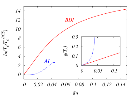
Figure 3: (Color on line) Comparison of SC $T_{c}$ for BDI and AI classes. In both cases all the initial parameters are zero except $\gamma_{c}^{0}(0)=-0.05$. The increase of $T_{c}$ in the AI case (blue-dashed line, in agreement with Ref. burmistrov ) stops entering the Anderson insulating regime (where $g$ diverges, see the corresponding blue-dashed line in the inset) while $T_{c}$ in the BDI case keeps on increasing with $g_{0}$ (red solid line).

V Conclusions

Interestingly, we have found a strong enhancement of the superconducting critical temperature, Eq. (12), for BDI class of two-sublattice models in two-dimensions (like a honeycomb), usually characterized by electron systems at half filling with a random hopping, which are not Anderson insulators. $T_{c}$ can be even larger than that obtained in the AI standard case for Anderson insulators burmistrov (see Appendix and Fig. 3), usually obtained by on-site disorder, going out of half-filling or breaking somehow the sublattice symmetry. In the BDI case, the dominant corrections to $T_{c}$ are given by the rescaling of the dynamical exponent (or, in other words, of the density of states). On the contrary, in the AI case, $z=d$, therefore $\eta=0$, and the increase of $T_{c}$ originates from an equation similar to Eq. (9), where $\eta$ is replaced by $g$, strongly renormalized by Anderson quantum interference corrections. Finally for a system at the Anderson transition (two- and three-dimensional (3D) symplectic class and 3D orthogonal class) $\eta$ is replaced by the fractal exponent $d_{2}$, getting a power-law enhancement of $T_{c}$ kravtsov . The importance of studying the two-sublattice systems is also the appearance of other instabilities such as charge-density wave or antiferromagnetic order induced by disorder. Moreover, the great advantage of such systems with random hopping, belonging to BDI class, as compared to the standard case with on-site disorder, is that the superconducting $T_{c}$ can be increased at will (at least within the validity of one-loop calculation, i.e. for $g_{0}\lesssim 1$) by tuning disorder and residual repulsive interaction, since superconductivity cannot be broken by entering any Anderson insulating phase (see Fig. 3).

VI Acknowledgements

The author acknowledges financial support from MIUR (“ArtiQuS”, FIRB 2012 RBFR12NLNA_$002$), thanks SISSA, Trieste, for hospitality and A. Trombettoni for useful discussions.

VII Appendix

Appendix A Extended Finkel’stein non-linear $\sigma$ model

The effective low-energy model which describe transverse charge fluctuations, derived in analogy with the original Finkel’stein model finkelstein , is the following npb

$$S=S_{0}+S_{I}\,,$$ (16)

where $S_{0}$ is the non-interacting part

$$S_{0} = \frac{\pi}{32}\int d{\bf r}\,\left\{\sigma\,\mathrm{Tr}\left(\vec{\nabla}Q\cdot\vec{\nabla}Q^{\dagger}\right)\right.-{8\nu Z}\,\mathrm{Tr}\left(\hat{\omega}Q\right)$$ (17)

$$\left.-\frac{\Pi}{8}\,\mathrm{Tr}\left(Q^{\dagger}\vec{\nabla}Q\rho_{3}\right)\cdot\mathrm{Tr}\left(Q^{\dagger}\vec{\nabla}Q\rho_{3}\right)\right\},$$

and $S_{I}$ the contribution from $e$-$e$ interactions

$$S_{I}=\frac{\pi^{2}\nu^{2}}{32}\int^{\prime}\Big{\{}\Gamma^{\alpha}_{t}\sum_{\beta=0,3}\mathrm{tr}(Q^{ii}_{n,n+p}\vec{S}_{\alpha\beta})\cdot\mathrm{tr}(Q^{ii}_{\ell+p,\ell}\vec{S}_{\alpha\beta})$$

$$-\Gamma^{\alpha}_{s}\sum_{\beta=0,3}\mathrm{tr}(Q^{ii}_{n,n+p}S^{0}_{\alpha\beta})\,\mathrm{tr}(Q^{ii}_{\ell+p,\ell}S^{0}_{\alpha\beta})$$

$$+\Gamma^{\alpha}_{c}\sum_{\beta=1,2}\mathrm{tr}(Q^{ii}_{n+p,-n}S^{0}_{\alpha\beta})\,\mathrm{tr}(Q^{ii}_{\ell+p,-\ell}S^{0}_{\alpha\beta}\Big{\}}$$ (18)

The symbol $\int^{\prime}$ in Eq. (18) means an integral over real space, a sum over smooth ($\alpha=0$) and staggered ($\alpha=3$) modes, $n_{r}$ replica indices and Matsubara frequencies, i.e. $\int^{\prime}\equiv\int d{\bf r}\sum_{\alpha=0,3}\sum_{i}\sum_{\ell,n,p}$, where $i$ is the replica index and $\ell,n,p$ are Matsubara indices. The matrix field $Q$ is constrained by the condition $QQ^{\dagger}=\mathbb{I}$. The coupling $\sigma$ corresponds to the Kubo formula for the charge conductivity at the Born level; $\nu$ is the density of states at the Fermi energy at the Born approximation; $\Gamma^{0}_{s},\Gamma^{0}_{t},\Gamma^{0}_{c}$ and $\Gamma^{3}_{s},\Gamma^{3}_{t},\Gamma^{3}_{c}$ are related to the Landau scattering amplitudes belitz or to the interaction parameters of a bipartite Hubbard-like model ludwig ($-t\sum c^{\dagger}_{Ai}c_{Bj}+h.c.+U\sum(n_{Ai}n_{Ai^{\prime}}+n_{Bj}n_{Bj^{\prime}})+V\sum n_{Ai}n_{Bj}$), for smooth ($\Gamma^{0}\sim(U+V)$) and staggered sublattice ($\Gamma^{3}\sim(U-V)$) components, in the particle-hole singlet, particle-hole triplet and particle-particle Cooper channels, respectively; $Z$ is the field renormalization constant; $\hat{\omega}$ is a diagonal matrix made of Matsubara frequencies. The last term in Eq. (17) is the anomalous additional term which is present only if the sublattice symmetry is preserved gade and the coupling $\Pi$ is related to the staggered density of states fluctuations michele . $\vec{S}_{\alpha\beta}$ is a vector made of three tensor products, i.e. $\vec{S}_{\alpha\beta}=\rho_{\alpha}\otimes\tau_{\beta}\otimes\vec{\sigma}$, while $S^{0}_{\alpha\beta}=\rho_{\alpha}\otimes\tau_{\beta}\otimes\sigma_{0}$ is a single tensor; $\tau_{1},\tau_{2},\tau_{3}$ are Pauli matrices in particle-hole space; $\sigma_{1},\sigma_{2},\sigma_{3}$ are Pauli matrices in spin space; $\rho_{3}$ is the third Pauli matrix in the sublattice space; $\tau_{0},\sigma_{0},\rho_{0}$ are identity matrices in the corresponding spaces. The trace “$\mathrm{Tr}$” is made over all spaces (particle-hole, spin, sublattice, replica and Matsubara spaces), while the trace “$\mathrm{tr}$” is over particle-hole, spin and sublattice spaces. The action in Eqs. (16)-(18) is tailored to describe two-sublattice models, namely when sublattice symmetry is preserved and staggered modes are massless. When the sublattice symmetry is broken, staggered modes become massive, then the last term in Eq. (17) and the terms in Eq. (18) with $\alpha=3$ should be put to zero ($\Pi=\Gamma_{s}^{3}=\Gamma_{t}^{3}=\Gamma_{c}^{3}=0$). In this way one recovers the standard Finkel’stein non-linear $\sigma$-model finkelstein , provided that $Q$ takes values in the proper coset space. If, instead, staggered modes are massless, those interacting terms are naturally generated by the RG flow.
In order to get rid of the field renormalization parameter, it is usually convenient to define the following parameters: $g\equiv 1/(2\pi^{2}\sigma)$, $\Gamma\equiv\Pi/(\sigma+n_{r}\Pi)$, $\gamma^{\alpha}_{s}\equiv 2\nu\Gamma^{\alpha}_{s}/Z$, $\gamma^{\alpha}_{t}\equiv 2\nu\Gamma^{\alpha}_{t}/Z$, $\gamma^{\alpha}_{c}\equiv 2\nu\Gamma^{\alpha}_{c}/Z$.

Appendix B RG equations - BDI class in the particle-hole symmetric case

In the presence of sublattice symmetry and imposing the particle-hole invariance by

$$\gamma^{0}_{s}=\gamma_{c}^{3}=-\gamma_{t}^{0}\equiv\gamma$$ (19)

$$\gamma^{3}_{s}=\gamma_{c}^{0}=-\gamma_{t}^{3}\equiv\bar{\gamma}$$ (20)

Eqs. (1-8) reported in the Letter reduce simply to

$$\frac{dg}{d\ell}=-\epsilon g+3g^{2}\left\{2\left(1+\frac{1-\gamma}{\gamma}\ln(1-\gamma)\right)-\bar{\gamma}\right\}$$ (21)

$$\frac{d\Gamma}{d\ell}=\epsilon\Gamma+8g+\frac{\Gamma}{g}\frac{dg}{d\ell}$$ (22)

$$\frac{d\gamma}{d\ell}=g\left\{\left(1-\gamma\right)\left(\frac{\Gamma}{8}+3\bar{\gamma}\right)+2\bar{\gamma}^{2}\right.$$ (23)

$$\phantom{d\gamma}\left.+(1-\gamma)^{2}\left(\frac{\Gamma}{4}\bar{\gamma}-4\bar{\gamma}-\frac{\Gamma}{8}\right)\right\}$$

$$\frac{d\bar{\gamma}}{d\ell}=g\left\{\bar{\gamma}\left(\frac{\Gamma}{8}+2\ln(1-\gamma)+3(\gamma+\bar{\gamma})\right)\right.$$ (24)

$$\phantom{d\bar{\gamma}}\left.+\left(\frac{\Gamma}{4}-1\right)\gamma\right\}-\bar{\gamma}^{2}$$

For $|\gamma|\ll|\bar{\gamma}|$ we have $d\gamma/d\ell\simeq g\left((\Gamma/4-1)\bar{\gamma}+\gamma\Gamma/8\right)$ and $d\bar{\gamma}/d\ell\simeq g\left(\bar{\gamma}\Gamma/8+(\Gamma/4-1)\gamma\right)-(\bar{\gamma})^{2}$. For $g_{0}\ll|\bar{\gamma}|$ and $\Gamma_{0}\simeq 0$, neglecting $\gamma$, we get the following critical temperature

$$T_{c}\sim\exp\left(-\frac{1}{|\bar{\gamma}|}\left(1-\frac{g_{0}^{2}}{6|\bar{\gamma}|^{2}}\right)\right),$$ (25)

namely, $\ln T_{c}$ increases quadratically with $g_{0}$. For sufficiently strong disorder, $g_{0}\gg|\bar{\gamma}|$, the critical temperature goes like $T_{c}\sim\exp\left(-\frac{{\cal C}}{g_{0}}\right)$, as in the general case treated in the Letter. It is worth stressing that, in the particle-hole symmetric case fixed by Eqs. (19-20), AFM, CDW and SC occur simultaneously.

B.1 RG equation in the standard case - AI class

If we break the sublattice symmetry, by going far from half-filling or in the presence of on-site impurities, we obtain the one-loop Finkel’stein equations, not restricted to long range Coulomb case finkelstein , at all orders in the interaction strenghts,

$$\frac{dg}{d\ell}=-\epsilon g+g^{2}\left\{5+\frac{1-\gamma_{s}^{0}}{\gamma_{s}^{0}}\,\ln(1-\gamma_{s}^{0})-3\,\frac{1+\gamma_{t}^{0}}{\gamma_{t}^{0}}\,\ln(1+\gamma_{t}^{0})-\gamma_{c}^{0}\right\}$$ (26)

$$\frac{d\gamma_{s}^{0}}{d\ell}=g\left\{\left(1-\gamma_{s}^{0}\right)\left(\frac{3}{2}\gamma_{t}^{0}+\gamma_{c}^{0}-\frac{1}{2}\right)+\frac{1}{2}\left(1-\gamma_{s}^{0}\right)^{2}+2(\gamma_{c}^{0})^{2}\right\}$$ (27)

$$\frac{d\gamma_{t}^{0}}{d\ell}=g\left\{\left(1+\gamma_{t}^{0}\right)\left(\frac{1}{2}\gamma_{s}^{0}-\gamma_{c}^{0}-\frac{1}{2}\right)+\left(1+\gamma_{t}^{0}\right)^{2}\left(\frac{1}{2}+2\gamma_{c}^{0}\right)\right\}$$ (28)

$$\frac{d\gamma_{c}^{0}}{d\ell}=g\left\{\frac{\gamma_{s}^{0}}{2}+\frac{3}{2}\gamma_{t}^{0}+\gamma_{c}^{0}\left(\frac{\gamma_{s}^{0}}{2}-\frac{3}{2}\gamma_{t}^{0}+\gamma_{c}^{0}+\ln\left[\frac{(1+\gamma_{t}^{0})^{3}}{(1-\gamma_{s}^{0})}\right]\right)\right\}-\left(\gamma_{c}^{0}\right)^{2}$$ (29)

which reduce to the equations reported in Ref. burmistrov , if only first orders in the $\gamma$’s are considered. In this case, for $\epsilon=0$, and $g_{0}\gg|\gamma_{c}^{0}(0)|$, one recovers the result burmistrov

$$T_{c}\sim\exp{(-1/g_{0})}\,.$$ (30)

Solving now the full set of Eqs. (26-29), we can show that, under increasing the bare repulsive interaction, $\gamma_{s}^{0}(\ell=0)$, $T_{c}$ decreases, and calculate the values of $\gamma_{s}^{0}(0)$ for which $T_{c}>T_{c}^{BCS}$ or $T_{c}<T_{c}^{BCS}$, as shown by Fig. 4.

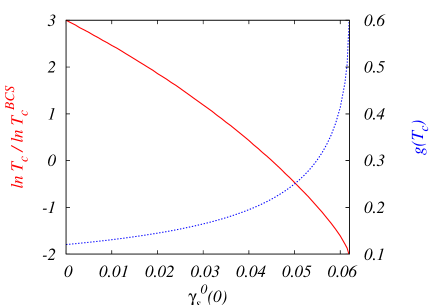
Figure 4: (Color online) Critical temperature (red-solid line), in log-scale, for AI class, in units of $T_{c}^{BCS}$ as a function of the initial value for $\gamma_{s}^{0}(0)$, at $\epsilon=0$, obtained for the following starting parameters: $g_{0}=0.03$, $\gamma_{t}^{0}(0)=0$, and $\gamma_{c}^{0}=-0.04$. For the same parameters $g(T=T_{c})$ is plotted (blue dashed line) as a function of the starting values $\gamma_{s}^{0}(0)$.

References

• (1) P.W. Anderson, Phys. Rev. 109, 1492 (1958).
• (2) P.W. Anderson, J. Phys. Chem. Solids 11, 26 (1959).
• (3) M. Ma and P.A. Lee, Phys. Rev. B 32, 5658 (1985).
• (4) A. Kapitulnik and G. Kotliar, Phys. Rev. Lett. 54, 473 (1985).
• (5) S. Maekawa, H. Fukuyama,J. Phys. Soc. Jpn. 51 1380 (1982).
• (6) A.M. Finkel’shtein, Zh. Eksp. Teor. Fiz. 84 168 (1983); Sov. Phys. JETP 57 97 (1983); A.M. Finkel’stein, Z. Phys. B 56 189 (1984).
• (7) M.V. Feigelman, L.B. Ioffe, V.E. Kravtsov, E.A. Yuzbashyan, Phys. Rev. Lett. 98 027001 (2007).
• (8) M.V. Feigelman, L.B. Ioffe, V.E. Kravtsov, E. Cuevas, Ann. Phys. 325 1390 (2010).
• (9) I.S. Burmistrov, I.V. Gornyi, A.D. Mirlin, Phys. Rev. Lett. 108, 017002 (2012)
• (10) R. Gade, F. Wegner, Nucl. Phys. B 360 213 (1991); R. Gade, Nucl. Phys. B 398 499 (1993).
• (11) C. Pepin, P.A. Lee, Phys. Rev. Lett. 81, 2779 (1998).
• (12) F.J. Wegner Z. Phys. B 35, 207 (1979).
• (13) K.B. Efetov, A.I.Larkin, and D.E. Khmel’nitskii, Zh. Eksp. Teor. Fiz. 79, 1120 (1979); Sov. Phys. JETP 52, 568 (1980).
• (14) C. Castellani, C. Di Castro, P.A. Lee, M. Ma, S. Sorella, E. Tabet, Phys. Rev. B 30, 1596 (1984).
• (15) D. Belitz, T.R. Kirkpatrick, Rev. Mod. Phys. 66, 261 (1994).
• (16) M. R. Zirnbauer, J. Math. Phys. 37, 4986 (1996).
• (17) F. Evers, Mirlin, Rev. Mod. Phys. 80, 1355 (2008).
• (18) In the symmetry classification of disordered systems the Cartan symbol AI refers to GOE (Gaussian orthogonal ensemble) random matices and the $\sigma$-model target space is $Sp(2n)/Sp(n)\times Sp(n)$ (in the replica formulation, $n\rightarrow 0$). BDI is the chiral class for GOE random matrices, in the $\sigma$-model formulation it corresponds to the manifold $U(2n)/Sp(n)$.
• (19) M. Fabrizio, C. Castellani, Nucl. Phys. B 583 542 (2000).
• (20) L. Dell’Anna, Nucl. Phys. B 758 255 (2006).
• (21) M.S. Foster and A.W.W. Ludwig, Phys. Rev. B 77, 165108 (2008).
• (22) M.R. Beasley, J.E. Mooij, and T.P. Orlando, Phys. Rev. Lett. 42, 1165 (1979).
• (23) O. Motrunich, K. Damle, and D.A. Huse, Phys. Rev. B 65, 064206 (2002).
• (24) C. Mudry, S. Ryu, and A. Furusaki, Phys. Rev. B 67, 064202 (2003).
• (25) L. Dell’Anna, Nucl. Phys. B 750 213 (2006).
• (26) Find at http://arxiv.org/format/1306.4618 the source file of the FORTRAN code (RG.f) solving the RG equations for both BDI, Eqs. (1)-(II), and AI, Eqs. (26)-(29), cases.