State space modelling and data analysis exercises
in LISA Pathfinder

Abstract

LISA Pathfinder is a mission planned by the European Space Agency (ESA) to test the key technologies that will allow the detection of gravitational waves in space. The instrument on-board, the LISA Technology package, will undergo an exhaustive campaign of calibrations and noise characterisation campaigns in order to fully describe the noise model. Data analysis plays an important role in the mission and for that reason the data analysis team has been developing a toolbox which contains all the functionality required during operations. In this contribution we give an overview of recent activities, focusing on the improvements in the modelling of the instrument and in the data analysis campaigns performed both with real and simulated data.

^a Dipartimento di Fisica, Università di Trento and INFN, Gruppo Collegato di Trento, 38050 Povo, Trento, Italy
^b European Space Astronomy Centre, European Space Agency, Villanueva de la Cañada, 28692 Madrid, Spain
^c Albert-Einstein-Institut, Max-Planck-Institut für Gravitationsphysik und Universität Hannover, 30167 Hannover, Germany
^d APC UMR7164, Université Paris Diderot, Paris, France
^e Dipartimento di Ingegneria dei Materiali e Tecnologie Industriali, Università di Trento and INFN, Gruppo Collegato di Trento, Mesiano, Trento, Italy
^f Dipartimento di Ingegneria Meccanica e Strutturale, Università di Trento and INFN, Gruppo Collegato di Trento, Mesiano, Trento, Italy
^g Astrium GmbH, Claude-Dornier-Strasse, 88090 Immenstaad, Germany
^h European Space Technology Centre, European Space Agency, Keplerlaan 1, 2200 AG Noordwijk, The Netherlands
ⁱ Department of Physics and Astronomy, University of Birmingham, Birmingham, UK
^j UPC/IEEC, EPSC, Esteve Terrades 5, E-08860 Castelldefels, Barcelona, Spain
^k Astrium Ltd, Gunnels Wood Road, Stevenage, Hertfordshire, SG1 2AS, UK
^l Institut für Flugmechanik und Flugregelung, 70569 Stuttgart, Germany
^m School of Physics and Astronomy, University of Glasgow, Glasgow, UK
ⁿ ICE-CSIC/IEEC, Facultat de Ciències, E-08193 Bellaterra (Barcelona), Spain
^o Institut für Geophysik, ETH Zürich, Sonneggstrasse 5, CH-8092, Zürich, Switzerland

1 Introduction

LISA Pathfinder (LPF) (ref. Antonucci et al. (2012)) is the first step towards the detection of gravitational waves in space. The mission has been designed to test those key technologies required to detect gravitational radiation in space. In more concrete terms, the objective of this pioneering technology probe is to measure the differential acceleration between two free-falling test masses down to $3\times 10^{-14}\rm m/s^{2}/\sqrt{\rm Hz}$ at 3 mHz, with a measuring bandwidth from 1 mHz to 0.1 Hz. It is precisely in this low-frequency bandwidth where the observation of gravitational waves in space can clearly contribute to our understanding of the Universe, since the gravitational wave sky is expected to be rich in interesting astrophysical sources in the millihertz band.

The main instrument on-board is the LISA Technology Package (LTP), which comprises subsystems which address the different functional requirements of the satellite: the Optical Metrology Subsystem (OMS) (ref. Heinzel et al. (2004)), the Gravitational Reference Sensor (GRS) (ref. Dolesi et al. (2003)), the Data and Diagnostics Subsystem (DDS) (ref. Canizares et al. (2011)) and the drag-free and attitude control system (DFACS) (ref. Fichter et al. (2005)). All of them working in closed loop in order to keep the two test masses on-board undisturbed at the required level.

The LPF mission has a planned duration of 200 days, during which a sequence of calibration and noise investigation runs are planned. This compressed time schedule to achieve the scientific objectives was identified by the science team as having an important impact during mission operations, and for that reason a data analysis effort was started, which had to be parallel but in close contact with the hardware development.

In this contribution we give an overview of recent developments in the data analysis task. We will emphasise some recent developments, namely the usage of state space models to describe the LTP experiment and the exercises, both with real and simulated data, performed using the tools developed for the analysis of LISA Pathfinder.

2 The LTPDA toolbox

During flight operations, the LTP experiment will undergo a tight schedule of experiments with the final aim of achieving the required differential noise acceleration between test masses. Some experiments could be strongly dependent on the results of previous experiments. For instance, noise models will need to be updated after a noise investigation to improve the description of the forthcoming investigations. Hence, data analysis will require a low latency between telemetry reception and the interpretation of the results. In order to cope with this demanding operational scenario it was decided to develop a data analysis framework specifically for use in LISA Pathfinder, the so-called LTPDA toolbox, a MATLAB^© (www.mathworks.com) toolbox which gathers together all analysis tools that will be used to analyse data during LISA Pathfinder operations. The main characteristics of this tool are the following:

• The toolbox is object-oriented. The user creates different types of objects to perform the analysis, the most usual ones are analysis objects which act as data containers, but there are others to allow many other functionalities like miir objects to create infinite impulse response filters, pzmodel objects to create pole-zero models, etc. More details can be found in ref. Hewitson et al. (2009)

• Each object keeps track of the operations being applied to it. The object-oriented approach allows the adding of a history step each time a method in the toolbox is applied to a given object. That way, the object stores the history of operations being applied to it and, more importantly, this history can be used to re-run the entire analysis by any other user to cross-check the results.

• During flight operations, the telemetry will be received at the European Space Astronomy Center (ESAC) and then distributed to the different research institutions. The data analysis will be coordinated but spread between different centres around Europe. In order to ease the interchange of results, the toolbox provides the infrastructure to work through one or more database repositories.

• The data analysis tools found to be relevant for the mission are implemented as methods in the toolbox. The current list of methods cover topics like spectral estimators, parameter estimation methods, digital filters and transfer function modelling, time domain simulation, noise generation and data whitening, as well as standard pre-processing tools like data splitting, interpolation, de-trending, and re-sampling.

• The toolbox provides models for the different subsystems of LTP which the user can call to perform simulations or to estimate parameters for a given data set. We give some more detail on the modeling in section 2.1

• As a part of the infrastructure of the toolbox, the development team has implemented a series of unit tests for each of the different methods which are executed on a daily basis to prevent the inclusion of new changes that may impact on the correct behaviour of the toolbox. About 6000 of these tests are executed repeatedly. Before any formal release to ESA  more functional tests are run in order to check not only the individual blocks but also the toolbox as a whole.

A significant amount of effort has as well been put into the user manual in order to allow non-specialized users to implement their analysis using the toolbox. With the same purpose, the team has been running a series of training sessions, where users follow a guided tutorial to run standard analysis. These tutorials are available to any interested user in the toolbox’s documentation.

2.1 Modelling LISA Technology Package onboard LISA Pathfinder

Modeling the instrument and the dynamics of the satellite is an important task among the data analysis activities. The LPF will be a complex experiment orbiting around L1 with hundreds of parameters determining its performance and many noise contributions to be determined. Disentangling the different contributions and dependencies will rely on our ability to build accurate models of the subsystems, which also need to be flexible enough to be able to include new information that the team may obtain during operations.

The team has been developing two modelling schemes. In chronological order, the first one uses the transfer function of the system in the Laplace domain to encode the response of each subsystem. For instance, the interferometer measurement would be described as

$$\vec{o} = ({\mathbf{M}}\cdot{\mathbf{S}}^{-1}+{\mathbf{C}})^{-1}(-{\mathbf{C}}\,\vec{o}_{i}+\vec{g}_{n}+{\mathbf{D}}\cdot{\mathbf{S}}^{-1}\vec{o}_{n}),$$ (1)

where $\mathbf{M}$ is the dynamical matrix, $\mathbf{C}$ is the controller, and $\mathbf{S}$ stands for the sensing matrix, which translates the physical position of the test masses into interferometer readout, $\vec{o}$. Subindex $n$ stands for noise quantities, either sensing noise ($\vec{o}_{n}$) or force noise ($\vec{g}_{n}$) and subindex $i$ stands for the injected signals ($\vec{o}_{i}$). If we do not take into consideration the angular degrees of freedom, all of these will be 2-dimensional vectors with components referring to the $\mathrm{x}_{1}$ (test mass #1 displacement) and $\mathrm{x}_{\Delta}$ (differential displacement between test masses) channels respectively. The matrices describing the motion of the test masses read as

$$\mathbf{M} = \left(\begin{array}[]{cc}s^{2}+\omega^{2}_{1}+\frac{m_{1}}{m_{\rm SC}}\omega^{2}_{1}+\frac{m_{2}}{m_{\rm SC}}\omega^{2}_{2}&\frac{m_{2}}{m_{\rm SC}}\omega^{2}_{2}\\ \omega^{2}_{2}-\omega^{2}_{1}&s^{2}+\omega^{2}_{2}\end{array}\right),$$ (4)

$$\mathbf{C} = \left(\begin{array}[]{cc}G_{\rm df}\,H_{\rm df}&0\\ 0&G_{\rm sus}\,H_{\rm sus}\end{array}\right),$$ (7)

$$\mathbf{S} = \left(\begin{array}[]{cc}S_{11}&S_{12}\\ S_{21}&S_{22}\end{array}\right),$$ (10)

where $\omega_{1}$ and $\omega_{2}$ are the stiffness, coupling the motion of each test mass to the motion of the spacecraft; $G_{\rm df}$ and $G_{\rm sus}$ are constant factors acting as calibration factors of the controller, $H_{\rm df}(\omega)$ and $H_{\rm sus}(\omega)$. The latter encode the control laws of the loop; the elements in the $\mathbf{S}$ matrix can be considered calibration factors and cross-couplings in the interferometer. This type of model, based on transfer functions, have been shown to work successfully when applied to the modelling of noise sources (ref. Ferraioli et al. (2011)) or in parameter estimation (ref. Nofrarias et al. (2010); Congedo et al. (2012)).

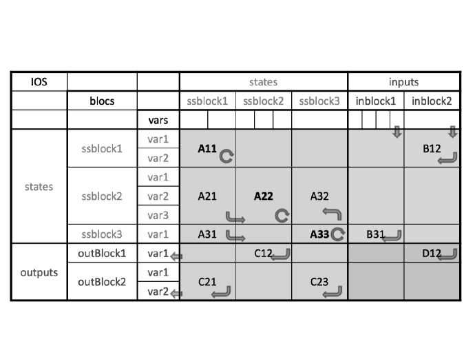
Figure 1.: A representation of a state space object in LTPDA. The ${\bf A}$, ${\bf B}$, ${\bf C}$ and ${\bf D}$ matrices are built in blocks. Each of these groups coefficients describing variables of the same nature. For instance, the diagonal block ${\bf A22}$ contains the dynamics of the variables of the states in block #2, but the ${\bf A32}$ describes the impact of the dynamics of states in block #3 on the states in block #2.

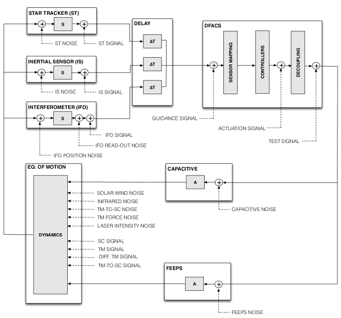
Figure 2.: A schematic representation of the LTP model. Each box is an independent state space model in LTPDA. In the figure we also show the noise and signal injection ports, which allow to input a noise model or an injection signal to the state space model, respectively.

The second approach to model LPF is based on the state space representation (ref. Kirk (1970)). This framework, widely used in control engineering, represents linear, time invariant, dynamic systems as matrices of time-independent coefficients.

$$\dot{\vec{x}}(t) = {\bf A}\cdot\vec{x}(t)+{\bf B}\cdot\vec{u}(t)$$

$$\vec{y}(t) = {\bf C}\cdot\vec{x}(t)+{\bf D}\cdot\vec{u}(t)$$ (11)

where $\vec{x}(t)$ are the so called states, i.e. variables describing the dynamical state of the system; $\vec{u}(t)$ represents the inputs and $\vec{y}(t)$ are the outputs of the system. The matrices relating them encode the coefficients of the first-order differential equations: $\bf A$ is the state matrix of the system, $\bf B$ is the input matrix, $\bf C$ is the output matrix and $\bf D$ is the feed-through matrix. This representation offers a fundamental advantage for the modelling of complex instruments such as LISA Pathfinder, which is its modularity. By describing each subsystem in the LTP as in equation (11), we are able to build high-dimensionality systems, and at the same time simplify the process of model validation. A second advantage is that the state space description makes our modelling easier to scale: the 1-dimensional models are built by selecting the relevant inputs, outputs and states of the complete 3-dimensional version.

In our implementation (ref. Grynagier (2009); Diaz-Aguilo (2011)), inputs, outputs and states are grouped into blocks with high level descriptions and global names. In that sense, the state space objects in LTPDA are block-defined, making easier to group together variables of similar nature –see Figure 1. The user is able to build models with multiple subsystems by assembling two state space models. For instance, one can choose to assemble a given model of the dynamics of the test masses with a model of the optical metrology subsystem or the gravitational reference sensor. In such a case, the assemble method would look in those models for input and output blocks with the same name and link those variables (or ports) that coincide in each of them.

Figure 2 shows the main subsystems of LISA Pathfinder implemented as state space models, and how these are connected between them when working in closed-loop. As an example, in Appendix A we show how to build a simplified state space model of the interferometer block. These blocks are already implemented in the LTPDA toolbox together with complete LPF built-in models, where all subsystems are already assembled in closed loop. Models are continuously being updated at the same time that new subsystems are added to our model library (ref. Gibert et al. (2012)).

3 Testing the LTPDA toolbox with data

Models and methods in LTPDA have been tested in several exercises with real and simulated data. In the following we provide and overview of those, and give the interested reader some references where to find more details.

3.1 Simulated data: the operational exercises

The first attempts to test the LTPDA tool against a real operations scenarion were organized as mock data challenges, following the concept previously applied to LISA data analysis (ref. Arnaud et al. (2006)). In these, the team is split into data generation and data analysis in such a way that the latter faces the data analysis task without the complete knowledge of the parameters and settings defining the model used to generate the data, as it will happen during mission operations. The first LPF mock data challenge dealt with a basic, albeit fundamental operation for the mission: the translation from displacement to acceleration (ref. Ferraioli et al. (2009); Monsky et al. (2009)). In this first exercise, the model was agreed between data generation and data analysis groups. On the contrary, the second mock data challenge was based on an unknown model of the satellite for the data analysis and so parameter estimation techniques had to be applied (ref. Nofrarias et al. (2010)), at the same time that the data generation techniques were improved (ref. Ferraioli et al. (2010)).

After these initial efforts, the following data analysis exercises changed the objective of the activity: mock data challenge were substituted by operational exercises ( ref. Antonucci et al. (2011)). The first relevant difference is that the OSE (Off-line Simulatons Environment), a detailed LISA Pathfinder non-linear simulator, is used to produce the data. Also, the aim of the operational exercises is to validate the experiments to be run on-board the satellite. In that sense, the operational exercises verify that the planned list of experiments are ready to be executed at the tele-command level. This list –put forward by the scientific team– contains experiments to characterise the optical metrology (ref. Audley et al. (2011)) and the inertial sensor instrument (ref. Dolesi et al. (2003)); thermal (ref. Canizares et al. (2011)) and magnetic studies (ref. Diaz-Aguilo et al. (2012)), and also pure free-fall experiments that aim at disentangling the contribution from actuators from the total noise budget (ref. Grynagier et al. (2009)). A series of parameter estimation studies have been performed using the OSE data, showing that our tools and models are able to explain and extract physical information, even if the model that we use for the analysis is not the same as the one used to generate the data (ref. Congedo et al. (2012); Karnesis et al. (2012); Nofrarias et al. (2012)).

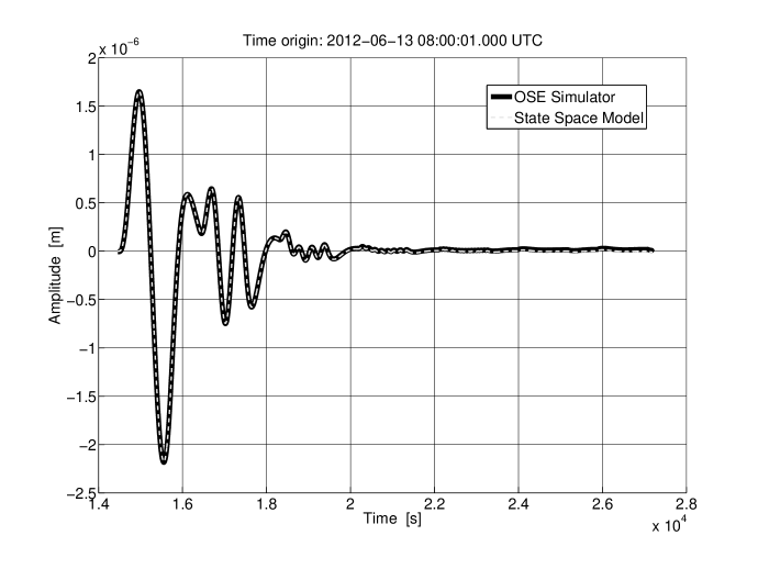
Figure 3.: Comparison between the OSE and state space model simulation. The same sinusoidal sequence is injected in the differential channel both in the OSE and in a LPF state space model, the injection point is the guidance signal in Figure 2. In the same scheme, the response shown here would be the output of the interferometer, after applying the delay block.

Recently, the team has started a series of mission simulation campaigns focusing on the data analysis constraints during operations. In the first mission simulation the team was split in two different locations, ESAC (Madrid) and APC (Paris), to force a coordinated effort between different sites. During the three days duration of the exercise, data –previously generated with the OSE– was received as in real operations: high priority (but low quality) telemetry in the morning and full telemetry at noon. That way, the team simulated an operations scenario where decisions based on the analysis results had to be taken on a daily basis. In Figure 3 we show a comparison between the OSE and the state space models obtained during this exercise. The LPF team plans to continue this activity increasing the degree of complexity in order to prepare for the real mission operations.

3.2 Real data: testing the satellite on-ground

Data analysis efforts have not only focused in simulated data. The tools and methods developed within the LTPDA toolbox are routinely used at the different laboratories both to test the toolbox functionality and also to get the scientific team familiarized with it. There have been several testing campaigns, for instance ref. Audley et al. (2011), where the toolbox has been used to analyse data from the real hardware.

As the launch draws nearer these test campaigns become more realistic, involving more subsystems assembled in the spacecraft. One of these was the space-craft closed loops test, performed at Astrium Ltd. premises. The focus here was to validate the ability of the space-craft to perform the science goals. However, the main instruments inside, like the optical metrology or the inertial sensor, where substituted by equipments simulating their operations. Communications and telemetry from the satellite platform where as in-flight operations and the whole processing chain underwent a realistic scenario.

A second testing campaign testing the real hardware was performed in the space simulator at IABG facilities. The so called On-Station Thermal Test (OSTT) was a twofold objective campaign, testing the operations of the optical metrology subsystem in a realistic space environment at the same time that the space-craft was subjected to a thermal balance test at two extreme temperature levels. More details on this campaign can be found in the following contribution on this volume  ref. Guzmán et al. (2012).

4 Summary

Given the complexity and the tight schedule, the in-flight operations of LISA Pathfinder will require a well coordinated and efficient data analysis, ready to react with a short time schedule once the data are received. Tools being developed in the LTPDA toolbox for that purpose are already in a mature state and the experiments to be performed on the satellite have been simulated and analysed with these methods.

In this contribution we have provided an overview of two of the many aspects involved in the data analysis of the LISA Pathfinder mission, i.e. the modelling and the data analysis exercises being performed to test the data analysis tools. On the modelling side, an important effort has been put forward to develop a framework that allows an efficient and flexible scheme to build models that will be afterwards used to understand the data from the satellite. These are currently implemented as state space models, which proved also to add advantages in terms of infrastructure maintenance.

The implemented data analysis tools have been tested with simulated data, mimicking the characteristics of the LISA Pathfinder data. Initially, these exercises focused on the development of data analysis algorithms. However, as the algorithms reached a mature state, the focus of the exercises moved to apply those algorithms to the experiments to be performed in flight. This is the main motivation behind what we call operational exercises. In parallel to these activities, the LPF mission has entered a phase of on-ground testing, which will be a perfect opportunity for the data analysis team to deal with real satellite data. Analysis and further results on these are currently ongoing and will be reported elsewhere.

Appendix

Appendix A A modelling example: a perfect interferometer model

Let’s assume that we are interested in modelling a perfect interferometer. This is, by itself, a complex instrument (ref. Heinzel et al. (2004)) but here we will be interested in the contribution of the interferometer to the dynamics of the satellite. In that sense, the interferometer must be understood as a sensor that translates the physical displacement of the test mass into a phase measurement from which an on-board algorithm calculates the actual attitude of the test mass which will be taken over by the DFACS controller as indicated in Figure 2.

In the transfer function description this information is captured in the S matrix. Hence, for an interferometer that does not add any cross-coupling this would turn into the identity matrix,

$$\mathbf{S} = \left(\begin{array}[]{cc}1&0\\ 0&1\end{array}\right)$$ (14)

On the other hand, in the state space model case, the system will be fully defined by the four matrices in equation (11). As in the previous case, we model the interferometer purely as a sensor and hence, it translates the input (the displacement of the test masses) to the interferometer output. The only matrix with non-zero coefficients is the $\bf D$ matrix, there is no contribution to the dynamics of the states by themselves ($\bf A$ matrix), neither coming from the inputs to the system ($\bf B$ matrix) or any dependence of the output with respect the states of the system ($\bf C$ matrix). A perfect interferometer model would be given by

$$\mathbf{A} = \left(\begin{array}[]{cc}0&0\\ 0&0\end{array}\right),\quad\mathbf{B}=\left(\begin{array}[]{cc}0&0\\ 0&0\end{array}\right),\quad\mathbf{C}=\left(\begin{array}[]{cc}0&0\\ 0&0\end{array}\right),$$ (21)

$$\mathbf{D} = \left(\begin{array}[]{cccc}\mathbf{D_{11}}&\mathbf{D_{12}}&\mathbf{D_{13}}&\mathbf{D_{14}}\\ \end{array}\right)$$ (23)

where the $\mathbf{D}$ matrix shows the block structure of our implementation that we have previously described. These matrices read as

$$\mathbf{D_{11}} = \left(\begin{array}[]{cc}1&0\\ -1&1\end{array}\right),\quad\mathbf{D_{12}}=\left(\begin{array}[]{cc}1&0\\ 0&1\end{array}\right),$$ (28)

$$\mathbf{D_{13}} = \left(\begin{array}[]{cc}1&0\\ -1&1\end{array}\right),\quad\mathbf{D_{14}}=\left(\begin{array}[]{cc}1&0\\ 0&1\end{array}\right)$$ (33)

and correspond to the four input blocks of the interferometer in our implementation, which will be, in corresponding order with the previous matrices

$$\vec{x} = \left(\begin{array}[]{c}x_{1}\\ x_{2}\end{array}\right),\quad\vec{n_{R}}=\left(\begin{array}[]{cc}n_{R1}\\ n_{R2}\end{array}\right),$$ (38)

$$\vec{n_{P}} = \left(\begin{array}[]{cc}n_{P1}\\ n_{P2}\end{array}\right),\quad\vec{s}=\left(\begin{array}[]{cc}s_{1}\\ s_{2}\end{array}\right)$$ (43)

which are: the test masses physical displacements ($\vec{x}$), the read-out interferometer noise ($\vec{n_{R}}$), the test mass position noise ($\vec{n_{P}}$), and an input block to inject signals in the interferometer ($\vec{s}$). The output of the interferometer will be the displacement of the test masses as translated in phase shifts. The output block, expressed as a vector, would be

$$\vec{o} = \left(\begin{array}[]{c}o_{1}\\ o_{\Delta}\end{array}\right)$$ (46)

where we notice that, opposite to the transfer function case, in the state space modelling the differential channel is built in the interferometer since the inputs to the interferometer were the displacements of the two test masses, $x_{1}$ and $x_{2}$.

References

- Antonucci et al. (2011) Antonucci, F., et al. 2011, Classical and Quantum Gravity, 28, 094006
- Antonucci et al. (2012) — 2012, Classical and Quantum Gravity, 29, 124014
- Arnaud et al. (2006) Arnaud, K. A., Babak, S., Baker, J. G., Benacquista, M. J., Cornish, N. J., Cutler, C., Larson, S. L., Sathyaprakash, B. S., Vallisneri, M., Vecchio, A., & Vinet, J.-Y. (Mock LISA Data Challenge Task Force and) 2006, AIP Conference Proceedings, 873, 619
- Audley et al. (2011) Audley, H., et al. 2011, Classical and Quantum Gravity, 28, 094003
- Canizares et al. (2011) Canizares, P., Chmeissani, M., Conchillo, A., Diaz-Aguiló, M., García-Berro, E., Gesa, L., Gibert, F., Grimani, C., Lloro, I., Lobo, A., Mateos, I., Nofrarias, M., Ramos-Castro, J., Sanjuán, J., Sopuerta, C. F., Araújo, H. M., & Wass, P. 2011, Classical and Quantum Gravity, 28, 094004
- Congedo et al. (2012) Congedo, G., Ferraioli, L., Hueller, M., De Marchi, F., Vitale, S., Armano, M., Hewitson, M., & Nofrarias, M. 2012, Phys. Rev. D, 85, 122004
- Diaz-Aguilo (2011) Diaz-Aguilo, M. 2011, Ph.D. thesis, Universitat de Politecnica de Catalunya
- Diaz-Aguilo et al. (2012) Diaz-Aguilo, M., Garcia-Berro, E., & Lobo, A. 2012, Phys. Rev. D, 85, 042004
- Dolesi et al. (2003) Dolesi, R., Bortoluzzi, D., Bosetti, P., Carbone, L., Cavalleri, A., Cristofolini, I., DaLio, M., Fontana, G., Fontanari, V., Foulon, B., Hoyle, C. D., Hueller, M., Nappo, F., Sarra, P., Shaul, D. N. A., Sumner, T., Weber, W. J., & Vitale, S. 2003, Classical and Quantum Gravity, 20, S99
- Ferraioli et al. (2011) Ferraioli, L., Congedo, G., Hueller, M., Vitale, S., Hewitson, M., Nofrarias, M., & Armano, M. 2011, Phys. Rev. D, 84, 122003
- Ferraioli et al. (2009) Ferraioli, L., Hueller, M., & Vitale, S. 2009, Classical and Quantum Gravity, 26, 094013
- Ferraioli et al. (2010) Ferraioli, L., Hueller, M., Vitale, S., Heinzel, G., Hewitson, M., Monsky, A., & Nofrarias, M. 2010, Phys. Rev. D, 82, 042001
- Fichter et al. (2005) Fichter, W., Gath, P., Vitale, S., & Bortoluzzi, D. 2005, Classical and Quantum Gravity, 22, S139
- Gibert et al. (2012) Gibert, F., Nofrarias, M., Diaz-Aguiló, M., Lobo, A., Karnesis, N., Mateos, I., Sanjuán, J., Lloro, I., Gesa, L., & Martín, V. 2012, Journal of Physics: Conference Series, 363, 012044
- Grynagier et al. (2009) Grynagier, A., Fichter, W., & Vitale, S. 2009, Classical and Quantum Gravity, 26, 094007
- Grynagier (2009) Grynagier, M., A. ; Weyrich 2009, The SSM class: modelling and analysis of the LISA Pathfinder Technology Experiment, Tech. rep., Institute of Flight Mechanics and Control, University of Stuttgart
- Guzmán et al. (2012) Guzmán, F., et al. 2012, ASD Conference Series, This Vol.
- Heinzel et al. (2004) Heinzel, G., Wand, V., García, A., Jennrich, O., Braxmaier, C., Robertson, D., K.Middleton, Hoyland, D., Rüdiger, A., Schilling, R., Johann, U., & Danzmann, K. 2004, Class. Quantum Grav., 21, 581
- Hewitson et al. (2009) Hewitson, M., et al. 2009, Class. Quant. Grav., 26, 094003
- Karnesis et al. (2012) Karnesis, N., Nofrarias, M., Sopuerta, C. F., & Lobo, A. 2012, Journal of Physics: Conference Series, 363, 012048
- Kirk (1970) Kirk, D. 1970, Optimal Control Theory: An Introduction (Prentice Hall Inc. Englewood Cliffs)
- Monsky et al. (2009) Monsky, A., et al. 2009, Class. Quant. Grav., 26, 094004
- Nofrarias et al. (2012) Nofrarias, M., Ferraioli, L., Congedo, G., Hueller, M., Armano, M., Diaz-Aguiló, M., Grynagier, A., Hewitson, M., & Vitale, S. 2012, Journal of Physics: Conference Series, 363, 012053
- Nofrarias et al. (2010) Nofrarias, M., Röver, C., Hewitson, M., Monsky, A., Heinzel, G., Danzmann, K., Ferraioli, L., Hueller, M., & Vitale, S. 2010, Phys. Rev. D, 82, 122002