The Mid-Infrared Extinction Law and its Variation in the Coalsack Nebula

Abstract

In recent years the wavelength dependence of interstellar extinction from the ultraviolet (UV), optical, through the near- and mid-infrared (IR) has been studied extensively. Although it is well established that the UV/optical extinction law varies significantly among the different lines of sight, it is not clear how the IR extinction varies among various environments. In this work, using the color-excess method and taking red giants as the extinction tracer, we determine the interstellar extinction $A_{\lambda}$ in the four Spitzer/IRAC bands in [3.6], [4.5], [5.8], [8.0]$\,{\rm\mu m}$ (relative to $A_{\rm K_{s}}$, the extinction in the 2MASS ${\rm K_{s}}$ band at 2.16$\,{\rm\mu m}$) of the Coalsack nebula, a nearby starless dark cloud, based on the data obtained from the 2MASS and Spitzer/GLIMPSE surveys. We select five individual regions across the nebula that span a wide variety of physical conditions, ranging from diffuse, translucent to dense environments, as traced by the visual extinction, the Spitzer/MIPS 24$\,{\rm\mu m}$ emission, and CO emission. We find that $A_{\lambda}/A_{\rm K_{s}}$, the mid-IR extinction relative to $A_{\rm K_{s}}$, decreases from diffuse to dense environments, which may be explained in terms of ineffective dust growth in dense regions. The mean extinction (relative to $A_{\rm K_{s}}$) is calculated for the four IRAC bands as well, which exhibits a flat mid-IR extinction law, consistent with previous determinations for other regions. The extinction in the IRAC 4.5$\,{\rm\mu m}$ band is anomalously high, much higher than that of the other three IRAC bands. It cannot be explained in terms of CO and CO₂ ices. The mid-IR extinction in the four IRAC bands have also been derived for four representative regions in the Coalsack Globule 2 which respectively exhibit strong ice absorption, moderate or weak ice absorption, and very weak or no ice absorption. The derived mid-IR extinction curves are all flat, with $A_{\lambda}/A_{\rm K_{s}}$ increasing with the decrease of the 3.1$\,{\rm\mu m}$ H₂O ice absorption optical depth $\tau_{\rm ice}$.

1 Introduction

1.1 Diffuse, Translucent, and Dense Clouds

The interstellar medium (ISM) is generally classified into three phases (see Snow & McCall 2006): the cold neutral medium (CNM), the warm ionized medium or warm neutral medium (WIM or WNM), and the hot ionized medium (HIM; also known as the intercloud medium or the coronal gas). The CNM itself contains a variety of cloud types (e.g., diffuse clouds, translucent clouds and molecular clouds), spanning a wide range of physical and chemical conditions. In diffuse clouds (e.g., sightlines toward $\zeta$ Oph and $\zeta$ Per) hydrogen is mostly in atomic form and carbon is mostly in ionized form (C⁺). They typically have a total visual extinction $A_{\rm V}\sim 0-1\,{\rm mag}$, a hydrogen number density $n_{\rm H}\sim 10-500\,{\rm cm}^{-3}$, and a gas temperature $T_{\rm gas}\sim 30-100\,{\rm K}$. In translucent clouds, hydrogen is mostly in molecular (H₂) and the transition of carbon from ionized (C⁺) to atomic (C) or molecular (CO) form takes place (e.g., the high latitude cirrus clouds, see Magnani et al.  1985). These clouds have $A_{\rm V}\sim 1-5\,{\rm mag}$, $n_{\rm H}\sim 500-5000\,{\rm cm}^{-3}$, and $T_{\rm gas}\sim 15-50\,{\rm K}$ and are thick enough for CO millimeter lines to be detectable. In molecular clouds (which are variously referred to as dense clouds, dark clouds, or dark molecular clouds) carbon becomes almost completely molecular (CO). They are cold (with $T_{\rm gas}\sim 10-15\,{\rm K}$), subject to large dust extinction (with $A_{\rm V}>5-10\,{\rm mag}$), and their densities typically exceed $10^{4}\,{\rm cm}^{-3}$. We note that dense cloud material is often surrounded by translucent material which, in turn, is often surrounded by diffuse cloud material.

Interstellar clouds become either diffuse, translucent or molecular, depending on the extent to which ultraviolet (UV) photons can penetrate into the clouds: with little extinction, diffuse clouds are almost fully exposed to the interstellar UV radiation so that nearly all molecules are destroyed by photodissociation (but also see Footnote 1), in molecular clouds where the large dust extinction highly attenuates the interstellar UV radiation, molecules are protected from being photodissociated, while translucent clouds fall in between these two extremes.

Dust plays a crucial role in governing the physical and chemical states of interstellar molecules and determining the physical and chemical structures of interstellar clouds. Apart from providing surfaces for the formation of some molecules (e.g., H₂), dust, through the scattering and absorption of starlight, controls the attenuation of UV radiation passing through the clouds and the depth to which UV radiation penetrates into the clouds. Hence dust extinction – the sum of absorption and scattering – is a crucial parameter in modeling the chemistry of interstellar clouds.

1.2 UV/Optical Extinction: Strong Dependence on Environments

The interstellar extinction law – the variation of extinction $A_{\lambda}$ with wavelength $\lambda$, usually expressed as $A_{\lambda}/A_{\rm V}$ – is known to vary significantly among sightlines in the UV/optical at $\lambda<0.7\,{\rm\mu m}$ (see Cardelli et al. 1989). Cardelli et al. (1989) found that the variation in the UV/optical can be described by a functional form (hereafter “CCM”) with only one parameter, $R_{\rm V}\,\equiv\,A_{\rm V}/E(B-V)$, the optical total-to-selective extinction ratio. The value of $R_{\rm V}$ depends upon the environment along the line of sight. A direction through diffuse, low-density regions usually has a rather low value of $R_{\rm V}$. The “average” extinction law for the Galactic diffuse clouds is described by a CCM extinction curve with $R_{\rm V}\approx 3.1$, which is commonly used to correct observations for dust extinction. Lines of sight penetrating into dense clouds, such as the Ophiuchus or Taurus molecular clouds, usually show $4<R_{\rm V}<6$ (see Mathis 1990). Theoretically, $R_{\rm V}$ may become infinity in dense regions rich in very large, “gray” grains (i.e., the extinction caused by these grains does not vary much with wavelength), while the steep extinction produced completely by Rayleigh scattering would have $R_{\rm V}\sim 1.2$ (Draine, 2003). A wide range of $R_{\rm V}$ values have been reported for extragalactic lines of sight, ranging from $R_{\rm V}\approx 0.7$ for a quasar intervening system at $z\approx 1.4$ (Wang et al. 2004) to $R_{\rm V}\approx 7$ for gravitational lensing galaxies (Falco et al. 1999).

1.3 Near-IR Extinction: A Universal Power Law?

With the wealth of available data from space-borne telescopes (e.g., ISO and Spitzer) and ground-based surveys (e.g., 2MASS) in the near- and mid-IR, in recent years we have seen an increase in interest in IR extinction. Understanding the effects of dust extinction in the IR wavelengths is important to properly interpret these observations.

As the UV/optical extinction varies substantially among various environments, one might expect the near-IR extinction at $0.9\,{\rm\mu m}<\lambda<3\,{\rm\mu m}$ to vary correspondingly. However, for over two decades astronomers have believed that there is little, if any, near-IR extinction variation from one line of sight to another. The near-IR extinction law appears to be an approximately uniform power law of $A_{\lambda}\sim\lambda^{-\alpha}$ with $\alpha$ $\approx$ 1.6–1.8, independent of environment or $R_{\rm V}$ at $0.9\,{\rm\mu m}<\lambda<3\,{\rm\mu m}$. The constancy of the near-IR extinction law implies that the size distribution of the large grains responsible for the near-IR extinction are almost the same in all directions. A “universal” power law also well describes the near-IR polarization $P_{\lambda}$ which, like the near-IR extinction, probes the large grain population, $P_{\lambda}/P_{\rm max}\propto\lambda^{-1.8}$, where $P_{\rm max}$ is the peak polarization (Martin & Whittet 1990).

However, much steeper power-laws have also been derived for the near-IR extinction. Stead & Hoare (2009) determined $\alpha\approx 2.14^{+0.04}_{-0.05}$ for the slope of the near-IR extinction power law for eight regions of the Galaxy between $l\sim 27^{\rm o}$ and $\sim 100^{\rm o}$. Nishiyama et al. (2009) explored the extinction law toward the Galactic center. They derived the index of the power law $\alpha\approx 1.99$. Fritz et al. (2011) found $\alpha\approx 2.11$ for the Galactic center extinction.

Based on a spectroscopic study of the 1–2.2$\,{\rm\mu m}$ extinction law toward a set of nine ultracompact HII regions with $A_{\rm V}>15\,{\rm mag}$, Moor et al. (2005) found some evidence that the near-IR extinction curve may tend to flatten at higher extinction, and no evidence of extinction curves significantly steeper than the standard law (even where water ice is present). Naoi et al. (2006) determined the near-IR color excess ratio $E({\rm J}-{\rm H})/E({\rm H}-{\rm K_{s}})$, one of the simplest parameters for expressing the near-IR extinction law, for L1688, L1689, and L1712 in the $\rho$ Oph cloud, and Cha I, Cha II, and Cha III in the Chamaeleon cloud. They found that $E({\rm J}-{\rm H})/E({\rm H}-{\rm K_{s}})$ changes with increasing optical depth, consistent with grain growth toward the inside of the dark clouds.

1.4 Mid-IR Extinction: Universally Flat?

The mid-IR extinction at $3\,{\rm\mu m}<\lambda<8\,{\rm\mu m}$ (in between the power-law regime at $\,{\sim}$1–3$\,{\rm\mu m}$ and the 9.7$\,{\rm\mu m}$ silicate Si–O stretching absorption feature) is not well understood. The determination of the mid-IR extinction law has been more difficult because this wavelength range is best accessed from space.

Rieke & Lebofsky (1985) argued that the near-IR power law of $A_{\lambda}\propto\lambda^{-1.61}$ extends out to $\,{\sim}$7$\,{\rm\mu m}$ before the extinction increases again toward the $9.7\,{\rm\mu m}$ silicate absorption peak. Bertoldi et al. (1999) and Rosenthal et al. (2000) studied the rotation-vibrational emission lines of H₂ of the Orion Molecular Cloud (OMC) obtained by ISO/SWS. They found that the relative line intensities of H₂ appear consistent with a power-law IR extinction of $A_{\lambda}\propto\lambda^{-1.7}$ extending from $\,{\sim}$2$\,{\rm\mu m}$ to $\,{\sim}$7$\,{\rm\mu m}$ (with an additional water ice absorption feature peaking at 3.05$\,{\rm\mu m}$).

However, based on the atomic H recombination lines toward Sgr A^∗ in the Galactic center obtained by ISO/SWS, Lutz et al. (1996) derived the extinction toward the Galactic center between 2.5$\,{\rm\mu m}$ and 9$\,{\rm\mu m}$ by comparing the observed and expected intensities of these lines. They found that the Galactic center extinction shows a flattening of $A_{\lambda}$ in the wavelength region of $3\,{\rm\mu m}<\lambda<9\,{\rm\mu m}$, clearly lacking the pronounced minimum in the $\,{\sim}$4–8$\,{\rm\mu m}$ region expected for the standard silicate-graphite model (see Draine 1989). This was later confirmed by Lutz (1999), Nishiyama et al. (2009), and Fritz et al. (2011).

Based on data from the 2MASS survey and the Spitzer/Galactic Legacy Infrared Mid-Plane Survey Extraordinaire (GLIMPSE) Legacy program, Indebetouw et al. (2005) determined the $\,{\sim}$1.25–8$\,{\rm\mu m}$ extinction laws photometrically from the color excesses of background stars for two very different lines of sight in the Galactic plane: $l=42\arcdeg$ which points toward a relatively quiescent region, and $l=284\arcdeg$ which crosses the Carina Arm and contains RCW 49, a massive star-forming region. The extinction laws $A_{\lambda}/A_{\rm K_{s}}$ derived for these two distinct Galactic plane fields are remarkably similar: both show a flattening across the 3–8$\,{\rm\mu m}$ wavelength range and lie above the curve extrapolated from $\lambda<3\,{\rm\mu m}$. They are consistent with that derived by Lutz et al. (1996) for the Galactic center, in spite of the large differences in method and sightlines. Even the low-density lines of sight in the Galactic midplane follow the same flat trend (see Zasowski et al. 2009).

Flaherty et al. (2007) obtained the mid-IR extinction laws in the Spitzer/IRAC bands for five nearby star-forming regions: the Orion A cloud, NGC 2068/71, NGC 2024/23, Serpens and Ophiuchus. The derived extinction laws at $\,{\sim}$4–8$\,{\rm\mu m}$ are flat, even flatter than that of Indebetouw et al. (2005). We note that almost all recent studies based on Spitzer/IRAC data show that the mid-IR extinction law for most regions departs from the power-law of $A_{\lambda}\propto\lambda^{-\alpha}$ (with $\alpha\sim$ 1.6–1.8) around 3$\mu$m and becomes flat until the silicate feature around 9.7$\,{\rm\mu m}$.

All these observations appear to suggest an “universal” extinction law in the mid-IR, with little dependence on environments. Chapman et al. (2009) computed the extinction law at 3.6–24$\,{\rm\mu m}$ for three molecular clouds: Ophiuchus, Perseus, and Serpens. However, they found that the shape of the mid-IR extinction law in all three clouds appears to vary with the total dust extinction: for $A_{\rm K_{s}}<0.5\,{\rm mag}$, the extinction law is well-fit by the WD01 $R_{\rm V}=3.1$ diffuse cloud dust model; as the extinction increases, it gradually flattens; for $A_{\rm K_{s}}>1\,{\rm mag}$, it becomes more consistent with the WD01 $R_{\rm V}=5.5$ model and that of Lutz et al. (1996) for the Galactic center.

Similar conclusions were drawn by McClure (2009) who used Spitzer/IRS observations of G0–M4 III stars behind dark clouds to construct empirical extinction laws at 5–20$\,{\rm\mu m}$ for $0.3<A_{\rm K_{s}}<7\,{\rm mag}$: for $A_{\rm K_{s}}<1\,{\rm mag}$ the extinction law appears similar to the $R_{\rm V}=3.1$ diffuse cloud extinction curve; for $A_{\rm K_{s}}>1\,{\rm mag}$, it lies closer to the WD01 $R_{\rm V}=5.5$ curve. McClure (2009) attributed the change of the shape of the IR extinction law (as well as the 9.7$\,{\rm\mu m}$ silicate absorption profile) to grain growth via coagulation and the presence of ice in dense molecular clouds (at $A_{\rm K_{s}}>0.5\,{\rm mag}$ or $A_{\rm V}>3\,{\rm mag}$; Whittet et al. 2001).

Cambrésy et al. (2011) explored the variations of the mid-IR extinction law within the Trifid nebula by measuring the extinction in the 3.6, 4.5, and 5.8$\,{\rm\mu m}$ Spitzer/IRAC bands. They found a flattening of the extinction law at a threshold of $A_{\rm V}\approx 20\,{\rm mag}$: below this threshold the extinction law is as expected from models for $R_{\rm V}=5.5$ whereas above $\,{\sim}$20$\,{\rm mag}$ of visual extinction, it is flatter.

Based on the data obtained from the Spitzer/GLIPMSE Legacy Program and the 2MASS project, Gao, Jiang, & Li (2009; hereafter GJL09) derived the extinction in the four IRAC bands (relative to the 2MASS ${\rm K_{s}}$ band) for 131 GLIPMSE fields along the Galactic plane within $|l|\leq 65^{\rm o}$, using red giants and red clump giants as tracers. As a whole, the mean extinction in the IRAC bands (normalized to the 2MASS ${\rm K_{s}}$ band) exhibits little variation with wavelength (i.e., somewhat flat or gray), consistent with the WD01 $R_{V}=5.5$ model extinction. As far as individual sightline is concerned, however, the wavelength dependence of the mid-IR interstellar extinction $A_{\lambda}/A_{\rm K_{s}}$ varies from one sightline to another. GLJ09 also demonstrated the existence of systematic variations of extinction with Galactic longitude which appears to correlate with the locations of spiral arms: the dips of the extinction ratios $A_{\lambda}/A_{\rm K_{s}}$ coincide with the locations of the spiral arms. GJL09 explained this in terms of the concentration of interstellar gas and dust at the inner edges of spiral arms which causes an increase of grain size and dust number density.

Using data from 2MASS and Spitzer/IRAC for G and K spectral type red clump giants, Zasowski et al. (2009) also found global longitudinal variations of the 1.2–8$\,{\rm\mu m}$ IR extinction over $\,{\sim}$150^o of contiguous Galactic mid-plane longitude; more specifically, they found strong, monotonic variations in the extinction law shape as a function of angle from the Galactic center, symmetric on either side of it: the IR extinction law becomes increasingly steep as the Galactocentric angle increases, with identical behavior between $l$ $<$ 180^o and $l$ $>$ 180^o.

However, other studies found no evidence for a flattening of the extinction law as a function of column density. Román-Zúñiga et al. (2007) obtained the extinction law $A_{\lambda}/A_{\rm K_{s}}$ between 1.25 and 7.76$\,{\rm\mu m}$ to an unprecedented depth in Barnard 59, a star-forming dense core located in the Pipe nebula, by combining sensitive near-IR data obtained with ground-based imagers on ESO NTT/VLT with space mid-IR data acquired with Spitzer/IRAC. However, they found no significant variation of the extinction law with depth. This has been confirmed by Ascenso et al. (2013) who derived the mid-IR extinction law toward the dense cores B59 and FeSt 1-457 in the Pipe nebula over a range of depths between $A_{\rm V}\sim 10\,{\rm mag}$ and $A_{\rm V}\sim 50\,{\rm mag}$, also using a combination of Spitzer/IRAC, and ESO NTT/VLT data. They found no evidence for a dependence of the extinction law with depth up to $A_{\rm V}\sim 50\,{\rm mag}$ in these cores. The mid-IR extinction law in both cores departs significantly from a power-law between 3.6 and 8$\,{\rm\mu m}$, suggesting that these cores contain dust with a considerable fraction of large dust grains.

1.5 This Work

As discussed in previous sections, it is now clear that the UV/optical/IR extinction varies from one sightline to another. This variation is mainly caused by the change of the grain size distribution in different environments. While the UV/optical extinction is relatively well understood, our understanding of the near- and mid-IR extinction is still somewhat poor and controversial, despite that in this spectral domain many advances have been made in the past few years. A better understanding of the regional variation of the near- and mid-IR extinction law will allow a more accurate reddening correction of the photometric and spectroscopic measurements. This is also crucial for a complete description of the varying dust properties across the Milky Way.

As summarized in §1.3, the IR extinction law is generally estimated in molecular clouds as a whole and the discrepancies between the different results are interpreted as variations of the dust properties from cloud-to-cloud due to the environment. However, most sightlines probably consist of a mixture of different types of clouds (e.g., a concentration of discrete clouds), instead of isolated, homogenous clouds. Within a cloud, the gas density is expected to increase from the envelope to the core and it is likely that a dense cloud has an “onion-like” structure, with dense cloud material in the center, surrounded by translucent gas, which is in turn surrounded by more diffuse gas. Therefore, the variation of the dust properties (and hence the extinction) within a cloud is expected. Dense clouds sample different physical conditions in the ISM and can be probed on large scales and for various astrophysical environments.

With the wealth of available deep data in the near- and mid-IR it is now possible to investigate the variation of the dust extinction within individual clouds. To reveal whether and how the mid-IR extinction law relates to the interstellar environment, in this work we explore the possible variations of the mid-IR extinction within the Coalsack nebula, a nearby starless dark cloud. We select individual regions across the nebula complex that span a wide variety of environments, from dense clouds to diffuse regions (see §2). Our analysis relies on the 2MASS and Spitzer/GLIMPSE surveys. Our method to derive the extinction law from 3.6 to 8.0$\,{\rm\mu m}$ is based on the “color-excess” method with red giants as the extinction tracer (see §3). We report in §4 the derived $A_{\lambda}/A_{\rm K_{s}}$, the extinction in the IRAC bands (relative to the 2MASS ${\rm K_{s}}$ band) for the selected regions, as well as the mean mid-IR extinction. In §5 we discuss the regional variations of the derived IR extinction. We summarize our major conclusions in §6.

2 The Coalsack Nebula

The Coalsack nebula is the most prominent, isolated dark cloud in the southern Milky Way (Tapia 1973, Bok 1977). Located around the Galactic longitude of $l\approx 303^{\circ}$ in the Galactic plane, it subtends an angle of $\,{\sim}$6^o in diameter on the sky. The distance to the Coalsack nebula is estimated to be $\,{\sim}$150 pc from photometric studies, which means a linear extent of $\,{\sim}$15 pc (see Cambrésy et al. 1999). It is characterized by complex, filamentary molecular structures which contain many dark cores and its total mass is estimated to be $\,{\sim}$3500 M_⊙ (see Nyman 2008). A cloud of this size and mass would be expected to contain young stars, but unlike other typical star-forming clouds such as Taurus and $\rho$ Ophiuchus, the Coalsack nebula appears completely devoid of star formation activity: it lacks the usual signposts of star formation activity, such as emission-line stars, Herbig-Haro objects, and embedded IR sources (Nyman et al. 1989, Bourke et al. 1995, Kato et al. 1999, Kainulainen et al. 2009). This suggests that the Coalsack nebula may be a young molecular cloud complex in the earliest stages of evolution. The globules within the Coalsack, including Tapia’s Globules 1, 2, and 3, the darkest and densest cores, are apparently all starless (and not centrally condensed) and may also be in the early phases of development. Moreover, the fraction of dense gas in the Coalsack complex is considerably smaller than that of typical star forming cloud complexes, as indicated by a ¹³CO emission line survey (Kato et al. 1999), also suggesting that the Coalsack nebula may not be forming stars.

The visual extinction $A_{\rm V}$ over the cloud varies between $\,{\sim}$1 and $\,{\sim}$3 mag (see Nyman 2008). Gregorio-Hetem et al. (1988) derived the average visual extinction of the cloud to be $A_{\rm V}\approx 5\,{\rm mag}$ through the method of star counts. However, $A_{\rm V}$ differs internally and can be much higher in small condensations and globules, reaching above 20$\,{\rm mag}$ in some regions (Tapia 1973, Bok 1977). The highest visual extinction in the cloud centering around ($l=301^{\circ},b=-1^{\circ}$) contains Tapia’s Globule 2, a potential star-forming region. With a large size and the complexity, the Coalsack nebula presents multiple environments, from opaque dense cores, translucent regions, to more extended diffuse components. Therefore, the Coalsack nebula is an ideal target for probing the regional variation of interstellar extinction.

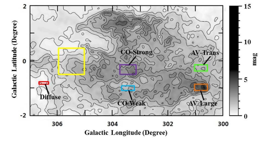
Figure 1: The visual extinction map of the Coalsack nebula of Dobashi et al. (2005). The resolution of the map is $\,{\sim}$6^′. Orange box: the “AV–Large” region which, with $A_{\rm V}>10\,{\rm mag}$, has the highest visual extinction in the map. Green box: the “AV–Trans” region for which the visual extinction is much lower (with $A_{\rm V}<3\,{\rm mag}$). Also marked are the other selected regions (see Figures 2, 3).

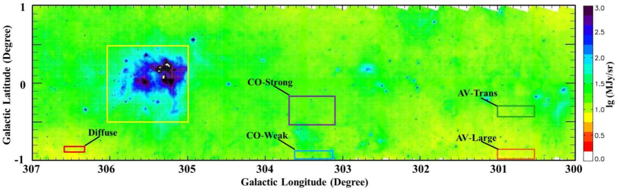
Figure 2: The Spitzer/MIPS 24$\,{\rm\mu m}$ image of the Coalsack nebula. The resolution of the mosaic image is $\,{\sim}$6^′ per pixel. The blue and violet filaments in the yellow box represent the brightest region in the 24$\,{\rm\mu m}$ emission map (however, it is not a part of the Coalsack nebula but a star-forming background cloud).

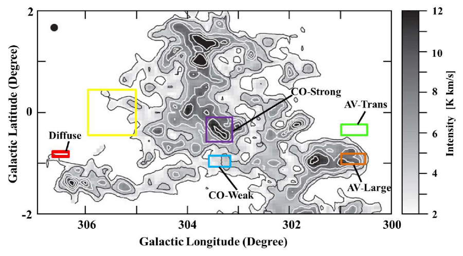
Figure 3: Map of the velocity-integrated CO (1-0) emission intensity of Coalsack (Nyman et al., 1989). Contours are from 2$\,{\rm K}\,{\rm km}\,{\rm s}^{-1}$ to 12$\,{\rm K}\,{\rm km}\,{\rm s}^{-1}$ in steps of 1$\,{\rm K}\,{\rm km}\,{\rm s}^{-1}$. Violet box: the “CO–Strong” region. Blue box: the “CO–Weak” region. The other selected regions are also marked.

To characterize the ISM environment, three maps of the Coalsack nebula are utilized independently: (i) the visual extinction map, (ii) the Spitzer/MIPS 24$\,{\rm\mu m}$ emission map, and (iii) the CO gas emission contour. Figures 1–3 display these maps of the Coalsack nebula for the selection of regions representative of different environments.

1. Visual Extinction ($A_{\rm V}$). The extinction depends on the dust column density $N_{\rm d}$ and the optical properties of the dust. Let $a$ be the mean grain size and $C_{\rm ext}(a,\lambda)$ be the extinction cross section of the dust of size $a$ at wavelength $\lambda$. The extinction is $A_{\lambda}=1.086\,N_{\rm d}\,C_{\rm ext}(a,\lambda)$. Apparently, a large $A_{\rm V}$ often implies a dense cloud (although it is also possible that it is just a pile-up of many diffuse clouds along the line of sight). Dobashi et al. (2005) presented a comprehensive catalog of dark clouds, in which the Coalsack nebula is labelled as No. 1867. Figure 1 is the $A_{\rm V}$ map around the Coalsack region with an angular resolution of $\,{\sim}$6^′ for which the lowest contour is 0.5 mag, with an interval of 0.5 mag in the range of $A_{\rm V}<3.0\,{\rm mag}$ and of 1.0 mag in the range of $A_{\rm V}>3.0\,{\rm mag}$. As described in §1.1, we distinguish different regions in terms of $A_{\rm V}$: (1) the region with the largest $A_{\rm V}$ ($>$ 10 mag), designated as “AV–Large” in Tables 1 and 2 and marked as an orange square in Figure 1, is chosen as a representative of dense clouds; (2) the region with moderate $A_{\rm V}$ ($<$ 3 mag), designated as “AV–Trans” in Tables 1 and 2 and marked as a green square in Figure 1, is chosen as a representative of translucent clouds.

2. Dust IR Emission. Let $T$ be the dust temperature (or the mean temperature averaged over a distribution of temperatures for stochastically heated dust). The dust emission intensity is $I_{\lambda}\propto N_{\rm d}\,C_{\rm abs}(a,\lambda)\,B_{\lambda}(T)$ where $B_{\lambda}(T)$ is the Planck function of temperature $T$ at wavelength $\lambda$. As the Coalsack nebula is starless, the dust is externally illuminated by the general interstellar radiation field. The dust in dense cores is colder than that in translucent or diffuse regions because of the attenuation of the external UV radiation. Therefore, regions bright in the IR must be dense. We adopt the Spitzer/MIPS 24$\,{\rm\mu m}$ image of the Coalsack nebula due to its high sensitivity and high spatial resolution. The brightest region marked as a yellow square in Figure 2, locating at $305.0^{\circ}<l<306.0^{\circ}$ and $-0.5^{\circ}<b<0.5^{\circ}$, is supposed to be very dense. However, it is not associated with the Coalsack nebula. It is a star-forming background cloud (see Clark & Porter 2004). Neither the “AV–Large” region nor the “AV–Trans” region exhibits appreciable 24$\,{\rm\mu m}$ emission.

3. CO Emission. In comparison with $A_{\rm V}$ and the 24$\,{\rm\mu m}$ dust emission, CO as a gas molecule is a relatively indirect tracer of dust. If the gas is well mixed with the dust as indicated by the tight correlation between the HI intensity and $A_{\rm V}$, the intensity of the CO emission lines should be proportional to the dust density (although this is complicated by the fact that the intensity of the CO emission line also depends on the excitation temperature). Indeed, Zasowski et al. (2009) used the ¹³CO (J = 1$\to$0) line to trace dense interstellar clouds (i.e., only dense gas can show up in the ¹³CO line emission). Figure 3 presents the integrated CO (1-0) intensity map of the Coalsack nebula with a resolution of $\,{\sim}$8^′ (Nyman et al., 1989). Complex structures are clearly seen in the CO map. Guided by the integrated CO line intensity map, we select two regions in the Coalsack nebula: the “CO–Strong” region which has the strongest line intensity (The CO emission line intensity can reach 6 K km/s), and the “CO–Weak” region which is weak in CO emission (The intensity of the CO emission line is less than 2 K km/s). These two regions should correspond to dense and translucent environments, respectively. They are marked as violet and blue squares in Figure 3, respectively.

As shown in Figure 3, the selections based on the visual extinction $A_{\rm V}$, the 24$\,{\rm\mu m}$ dust emission, and the CO emission are generally consistent, but discrepancy also exists. The “AV–Large” region is strong in the CO line emission, although not the strongest. The “AV–Trans” region is weak in CO emission: with an intensity of $\,{\sim}$1$\,{\rm K}\,{\rm km}\,{\rm s}^{-1}$ (see Figure 1 of Nyman et al. 1989) it does not show up in Figure 3 for which the lowest contour is 2$\,{\rm K}\,{\rm km}\,{\rm s}^{-1}$. All these regions do not seem to be very bright in the Spitzer/MIPS 24$\,{\rm\mu m}$ map (see Figure 2), especially the “CO–Strong” region or the “AV–Large” region. This is because the 24$\,{\rm\mu m}$ dust emission is not only proportional to the dust column density $N_{\rm d}$ but also non-linearly proportional to the dust temperature $T$, while $T$ depends on $N_{\rm d}$ as well: $T$ is lower in denser regions because of the attenuation of the illuminating interstellar UV radiation. Therefore, the densest regions (e.g., “AV–Large”) are not necessarily the brightest in the Spitzer/MIPS 24$\,{\rm\mu m}$ emission map because the darkest and densest cores have the lowest $T$. Because of this, the visual extinction $A_{\rm V}$ appears to be the best to characterize dense, translucent, and diffuse regions.

Finally, we select a diffuse region (designated “Diffuse”; see Figures 1–3) near the east edge of the Coalsack nebula where there is essentially no dust extinction ($A_{\rm V}<1\,{\rm mag}$; see Figure 1), very little CO emission (the intensity of CO emission is less than 1 K km/s), and undetectable 24$\,{\rm\mu m}$ emission (see Figure 3).

To summarize, in total five regions are selected (see Table 1): two dense regions (“AV–Large”, and “CO–Strong”), two translucent regions (“AV–Trans”, and “CO-Weak”) , and one diffuse region (“Diffuse”) within the Coalsack nebula. These regions cover various interstellar environments, from diffuse, translucent to dense.

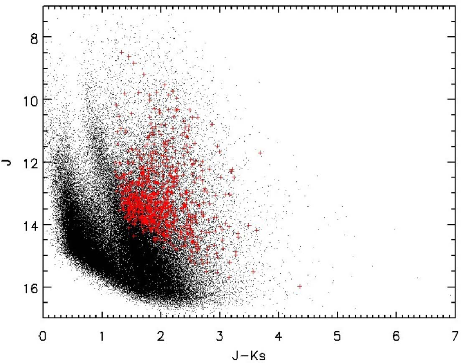
Figure 5: The $\left({\rm J}-{\rm K_{s}}\right)$ vs. ${\rm J}$ color-magnitude diagram for the “AV–Trans” region (see Figure 1 and Table 1). Black dots: all the sources in the GLMIC $l$300 field of GLIMPSE I which covers the “AV–Trans” region. Red crosses: the selected red giants of this region.

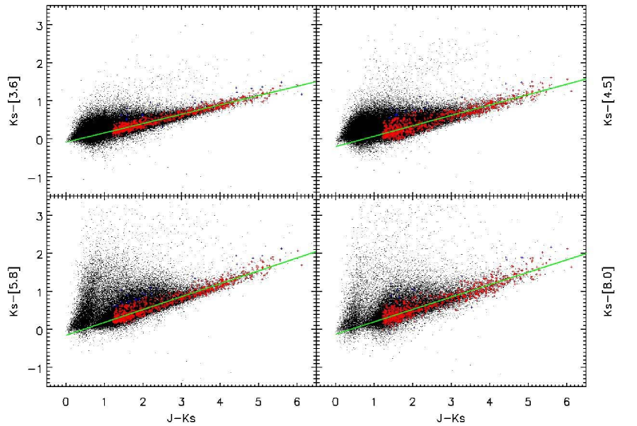
Figure 6: The 2MASS and Spitzer/IRAC color-color diagrams for the sources shown in Figure 5. Green lines: the best fits to the data. Blue points: the sources which are dropped based on a $3\sigma$ criterion.

We also note that the Coalsack nebula is located at a Galactic latitude close to $\,{\sim}0^{\rm o}$, for a selected sightline the extinction could be contaminated by background clouds. For example, the “AV–Trans” region, with $A_{\rm V}\lesssim 3\,{\rm mag}$ and $A_{\rm J}/A_{\rm K_{\rm s}}\approx 3.28$ (see §4 and Table 3), is expected to be reddened by an amount of $E({\rm J}-{\rm K_{s}})\approx 0.8\,{\rm mag}$ (assuming $A_{\rm V}/A_{\rm K_{\rm s}}\approx 8.5$), while Figures 5,6 show that the ${\rm J}-{\rm K_{s}}$ colors of some red giants in the “AV–Trans” region exceed $\,{\sim}$3$\,{\rm mag}$, implying that background clouds could contribute $\gtrsim$1$\,{\rm mag}$ to the reddening of these sources (assuming an intrinsic color of ${\rm J}-{\rm K_{s}}\approx 1.2\,{\rm mag}$ for red giants). To quantitatively estimate the contributions of background clouds to the extinction, we calculate the $E({\rm J}-{\rm K_{s}})$ values from $A_{\rm V}$ and compare them with that from the ${\rm J}$ vs. ${\rm J}-{\rm K_{s}}$ color-magnitude diagrams (e.g., see Figure 5). It is found that the extinction of the “Diffuse”, “AV–Large” and “CO–Weak” regions is mainly from these regions, with little contribution from background clouds, while the “CO–Strong” region is similar to the “AV–Trans” region, with background clouds contributing an additional reddening of $E({\rm J}-{\rm K_{s}})\gtrsim 2\,{\rm mag}$.

One can also gain insight into the possible background contamination by examining the CO components of the Coalsack nebula. In Figure 4 we show the CO velocity $V_{\rm LSR}$ vs. the CO line brightness (expressed as $T_{\rm A}$, the antenna temperature) for these five regions. It is clearly seen that the velocities at the “Diffuse”, “AV–Large” and “CO–Weak” regions have only one component at $\,{\sim}-5\,{\rm km}\,{\rm s}^{-1}$ which is from the Coalsack nebula.

In contrast, there are two velocity components toward both the “AV–Trans” and “CO–Strong” regions: one component peaks between $-10$ to 10$\,{\rm km}\,{\rm s}^{-1}$ that is supposedly from the Coalsack nebula; the other peaks from about $-40$ to $-20\,{\rm km}\,{\rm s}^{-1}$ which is definitely behind the Coalsack nebula. Nevertheless, for the “AV–Trans” sightline, the intensity of the CO line at $\,{\sim}-35\,{\rm km}\,{\rm s}^{-1}$ is comparable to that for the Coalsack nebula. This suggests that the background cloud may be in an environment similar to that of the “AV–Trans” region and therefore, it would have little effect on the extinction law of the “AV–Trans” region. As for the “CO–Strong” region, the peak intensity of the additional component is slightly weaker than that of the Coalsack nebula component, while the integrated intensity is comparable. The starlight intensity of the Coalsack nebula is likely weaker than that of the background cloud as the Coalsack is illuminated by the external interstellar radiation field, while the background is at least also excited by the general interstellar radiation field or even by an embeded or nearby star. Therefore, the CO–Strong region of the Coalsack nebula could be relatively denser than the background cloud and the dust properties derived for the CO–Strong region in this work could be contaminated by dust in an environment which is less dense. However, due to the lack of detailed knowledge of the radiation field of the background cloud, it is difficult to quantitatively assess this effect. Nevertheless, it is worth noting that the region was selected from the CO emission intensity map of Nyman et al. (1989) which was obtained by integrating the velocity from $-10$ to $8\,{\rm km}\,{\rm s}^{-1}$ for the coalsack nebula specifically, excluding the background cloud.

3 Methods and Tracers

3.1 The “Color-Excess” Method

The method of “color excess” is used to obtain the extinction as a function of wavelength. The details of the method can be found in GJL09. In brief, this method derives the extinction from the ratio of color excesses $E(\lambda_{r}-\lambda)$ and $E(\lambda_{c}-\lambda_{r})$, where $\lambda_{r}$ is the reference band, $\lambda_{c}$ the comparison band, $\lambda$ is the band investigated (i.e., the Spitzer/IRAC bands at [3.6], [4.5], [5.8], and [8.0]$\mu$m). In our study, we take the ${\rm K_{s}}$ band to be the reference band, and the J band to be the comparison band. Thus, the “color-excess” method calculates the ratio following

$$k_{x}\equiv\frac{E({\rm K_{s}}-\lambda)}{E({\rm J}-{\rm K_{s}})}=\frac{({\rm K_{s}}-\lambda)-({\rm K_{s}}-\lambda)_{0}}{({\rm J}-{\rm K_{s}})-({\rm J}-{\rm K_{s}})_{0}}=\frac{A_{\rm K_{s}}-A_{\lambda}}{A_{\rm J}-A_{\rm K_{s}}}~{}~{},$$ (1)

where $({\rm K_{s}}-\lambda)_{0}$ and $({\rm J}-{\rm K_{s}})_{0}$ are the intrinsic colors of the source. The relative extinction $A_{\lambda}/A_{\rm K_{s}}$ can then be derived from given $A_{\rm J}/A_{\rm K_{s}}$:

$$A_{\lambda}/A_{\rm K_{s}}=1+k_{x}(1-A_{\rm J}/A_{\rm K_{s}}).$$ (2)

Our method does not calculate the color excess ratio of individual stars, instead, it calculates the ratio of a group of stars. In practice, the color excess ratio $k_{x}$ is derived from the slope of a linear fitting of $E({\rm K_{s}}-\lambda)$ vs. $E({\rm J}-{\rm K_{s}})$. This statistical method reduces the uncertainty by increasing the number of sources involved. The key of this method lies in choosing a group of sources with homogeneous intrinsic color indices.

3.2 Data: 2MASS and Spitzer/GLIMPSE Surveys

The near- and mid-IR magnitudes of the objects are needed for the “color-excess” method. We obtain these data from the 2MASS PSC catalog (Skrutskie et al., 2006) and the Spitzer/GLIMPSE PSC catalog (Benjamin et al., 2003). The 2MASS PSC provides measurements in ${\rm J}$ (1.24$\mu$m), ${\rm H}$ (1.66$\mu$m), and ${\rm K_{s}}$ (2.16$\mu$m) bands in the whole sky. The GLIMPSE program is a mid-IR survey program of the inner Galactic plane in four filters ([3.6], [4.5], [5.8], [8.0]) using the IRAC camera onboard Spitzer. It has four cycles: GLIMPSE I, GLIMPSE II, GLIMPSE 3D and GLIMPSE 360 (Churchwell et al., 2009). Furthermore, the GLIMPSE PSC (version 2.0) has already cross-identified with the 2MASS PSC (see Cutri et al. 2003), bringing in great convenience to our work. Due to the orientation of the GLIMPSE survey, the PSC is confined to the Galactic latitude $b$ within $\pm 1^{\circ}$.

3.3 Selection of the Extinction Tracers

Red giants (RGs) are good tracers of interstellar extinction in the IR. They have a narrow range of effective temperatures and thus the scatter of their intrinsic color indices is small (e.g., the intrinsic $({\rm J}-{\rm K_{s}})$ color index of RGs is $\,{\sim}$1.2 mag with a scatter of only $\,{\sim}$0.1 mag; Bertelli et al. 1994; Glass et al. 1999). Moreover, RGs are bright in the IR (e.g., their absolute magnitude in the ${\rm K_{s}}$ band can reach $\,{\sim}$$-5.0$ mag; GJL09). In comparison, red clump stars (RCs) that are also often used as tracers of IR extinction have $M_{\rm K_{s}}\sim-1.65\,{\rm mag}$ (Wainscoat et al., 1992). This implies that RGs can trace a distance $\,{\sim}$5 times further than RCs. We adopt the following criteria to select RGs:

1. $[3.6]-[4.5]<0.6$ mag and $[5.8]-[8.0]<0.2$ mag. These restrictions exclude sources with intrinsic IR excesses from circumstellar dust (Flaherty et al., 2007) such as pre-main-sequence stars, asymptotic giant branch stars (AGBs) and young stellar objects (YSOs; Allen et al. 2004).

2. ${\rm J}-{\rm K_{s}}>$ 1.2 mag and ${\rm H}-{\rm K_{s}}>$ 0.3 mag. Marshall et al. (2006) found that the dwarf population is on the left side of the ${\rm K_{s}}$ vs. ${\rm J}-{\rm K_{s}}$ diagram, and the line near ${\rm J}-{\rm K_{s}}$ = 0.9 can be used to exclude dwarf stars. We follow GJL09 to adopt the (more restrict) criteria of ${\rm J}-{\rm K_{s}}>\,1.2$ and ${\rm H}-{\rm K_{s}}>\,0.3$ to exclude foreground dwarfs.

3. S/N $\geq$ 10. To guarantee the photometric quality, we only include the sources with S/N $\geq$ 10 in all seven bands (i.e., three 2MASS bands and four IRAC bands).

4. $<$ 3$\sigma$ deviation from the linear fitting. The objects selected according to the above criteria are taken to fit the ${\rm J}-{\rm K_{s}}$ vs. ${\rm K_{s}}-\lambda$ relation. Still, there are some sources with a deviation exceeding 3$\sigma$. These sources are rejected from a statistical point of view, also, most of them have large ${\rm K_{s}}-\lambda$ color excesses, suggesting the extinction may arise from circumstellar dust (Jiang et al., 2006).

Figure 5 shows the selected RG stars together with other stars (e.g., dwarfs, stars with IR excess) in the ${\rm J}-{\rm K_{s}}$ vs. ${\rm J}$ diagram for the “AV–Trans” region. The black dots are all the sources in the field GLMIC $l$300 of GLIMPSE I which covers the “AV–Trans” region. The selected RGs are marked as red crosses. The branches of the dwarf and red clump stars are clearly seen in this diagram, while those sources with intrinsic IR excess are mixed with RGs, although they have redder colors in the mid-IR bands.

4 Results

The calculation of $A_{\lambda}/A_{\rm K_{s}}$ from the color excess ratios $E({\rm K_{s}}-\lambda)/E({\rm J}-{\rm K_{s}})$ is straightforward (see eq. 2). Here the wavelength $\lambda$ refers to the Spitzer/IRAC bands at [3.6], [4.5], [5.8], [8.0]$\,{\rm\mu m}$. For each region listed in Table 1, $A_{\lambda}/A_{\rm K_{s}}$ is calculated based on the selected RGs and the linear fitting of ${\rm J}-{\rm K_{s}}$ vs. ${\rm K_{s}}-\lambda$. The number of RG stars that participate in the final linear fitting is shown in the last column of Table 1, all exceeding 100 sources. This guarantees that the “color-excess” method (see §3.1) to be statistically significant. Figure 6, as an example, illustrates this procedure for the “AV–Trans” region. During the linear fitting (to derive $k_{x}$, see eq. 1), those sources with a deviation exceeding 3$\sigma$ are dropped and such a fitting is repeated three times. The color excess ratios $E({\rm K_{s}}-\lambda)/E({\rm J}-{\rm K_{s}})$ for all the selected regions are shown in Table 2.

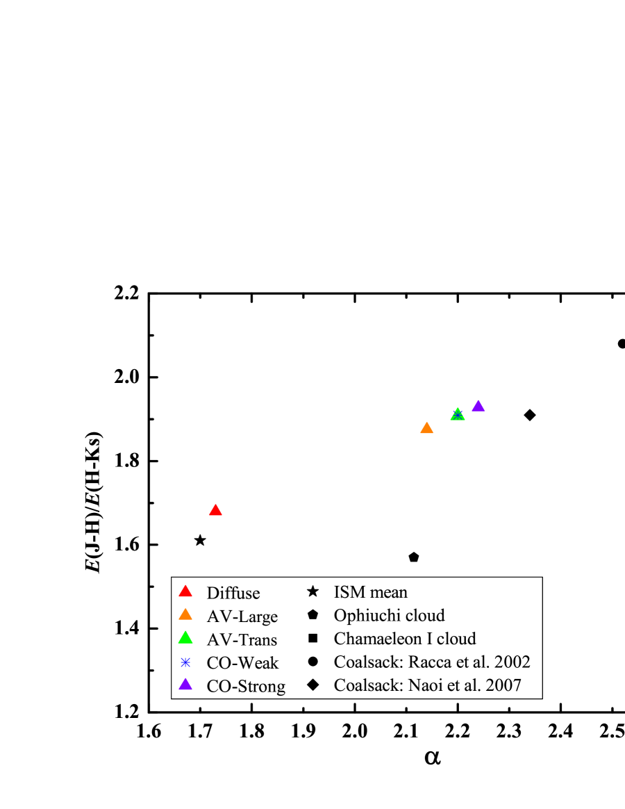
Figure 7: $E({\rm J}-{\rm H})/E({\rm H}-{\rm K_{s}})$ vs. $\alpha$ for all the five selected regions, where $\alpha$ is the power exponent of the near-IR extinction which is approximated as a power law $A_{\lambda}\propto\lambda^{-\alpha}$. Also shown are the $\alpha$ values estimated for the Ophiuchi cloud, the Chamaeleon I dark cloud (Kenyon et al. 1998, Gómez & Kenyon 2001) and the mean values averaged over diverse environments (Whittet 1988), as well as earlier determinations for the Coalsack nebula (Racca et al. 2002, Naoi et al. 2007).

In converting the color excess ratio $E({\rm K_{s}}-\lambda)/E({\rm J}-{\rm K_{s}})$ to the extinction ratio $A_{\lambda}/A_{\rm K_{s}}$ (see eq. 2), the knowledge of $A_{\rm J}/A_{\rm K_{s}}$ for each region is required. We therefore first derive $A_{\rm J}/A_{\rm K_{s}}$ for each region based on the 2MASS photometry. We also fit the 2MASS JHK_s extinction in terms of a power-law $A_{\lambda}\sim\lambda^{-\alpha}$ and derive the power exponent $\alpha$ for each region. In Table 3 we tabulate $A_{\rm J}/A_{\rm K_{s}}$ and $\alpha$ for all five regions. Except for the “Diffuse” region, all regions have $A_{\rm J}/A_{\rm K_{s}}\gtrsim 3.0$, exceeding by $>$20% that of Rieke & Lebofsky (1985) for stars in the Galactic center and of Indebetouw et al. (2005) for the $l=42^{\circ}$ and $l=284^{\circ}$ sightlines in the Galactic plane: $A_{\rm J}/A_{\rm K_{s}}\approx 2.52$. In Figure 7 we plot the near-IR color excess ratio $E({\rm J}-{\rm H})/E({\rm H}-{\rm K_{s}})$ over the near-IR extinction power exponent $\alpha$ for the selected five regions as well as for the Ophiuchi cloud, the Chamaeleon I dark cloud, and the mean values averaged over diverse environments (Kenyon et al. 1998, Gómez & Kenyon 2001, Whittet 1988a).

Except for the “Diffuse” region, the near-IR extinction laws for all other regions are rather steep, with $\alpha>2.0$ and reaching $\alpha\gtrsim 2.2$ for the “AV–Trans”, “CO–Weak”, and“CO–Strong” regions. In comparison, the typical value for interstellar clouds is $\alpha\sim 1.6-1.8$ (see §1.3), although $\alpha\gtrsim 2$ has also been reported for some regions (e.g., see Stead & Hoare 2009, Nishiyama et al. 2009; see §1.3). This confirms the earlier determination of Naoi et al. (2007) who derived $\alpha\approx 2.34\pm 0.01$ for the Coalsack Globule 2, based on observations made with the Simultaneous Infrared Imager for Unbiased Survey (SIRIUS) on the Infrared Survey Facility (IRSF) 1.4 m telescope at the South African Astronomical Observatory (SAAO).

Also except for the “Diffuse” region, the near-IR color excess ratios for all other regions, with $E({\rm J}-{\rm H})/E({\rm H}-{\rm K_{s}})>1.8$, are appreciably higher than the mean value of $1.61\pm 0.04$ averaged over diverse environments (Whittet 1988a). They are also higher than the ratios for the $\rho$ Ophiuchi cloud and the Chamaeleon I dark cloud ($E({\rm J}-{\rm H})/E({\rm H}-{\rm K_{s}})$ $\,{\sim}$1.6–1.7; see Kenyon et al. 1998, Gómez & Kenyon 2001). This confirms the earlier results of Naoi et al. (2007) who derived $E({\rm J}-{\rm H})/E({\rm H}-{\rm K_{s}})\approx 1.91\pm 0.01$ for the Coalsack Globule 2 for the extinction range $0.5<E({\rm J}-{\rm H})<1.8$. Racca et al. (2002) also observed the Coalsack nebula and determined $E({\rm J}-{\rm H})/E({\rm H}-{\rm K_{s}})\approx 2.08\pm 0.03$. Naoi et al. (2007) argued that steep near-IR extinction law and the large near-IR color excess ratio might indicate little growth of dust grains, or large abundance of dielectric non-absorbing components such as silicates, or both in the Coalsack Globule 2.

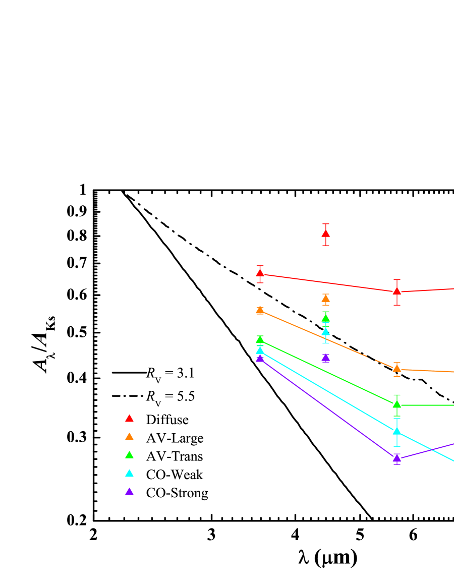
Figure 8: The mid-IR extinction $A_{\lambda}/A_{\rm K_{s}}$ of the five selected regions in the Coalsack nebula. For comparison, the WD01 $R_{\rm V}=3.1,5.5$ model extinction curves are also shown. The error bars in this figure and Figure 13 are derived from the linear fitting of $E({\rm K_{s}}-\lambda)/E({\rm J}-{\rm K_{s}})$.

With $A_{\rm J}/A_{\rm K_{s}}$ derived from the 2MASS dataset for each region, we determine the mid-IR extinction in the four IRAC bands (relative to that in the 2MASS ${\rm K_{s}}$ band) $A_{\lambda}/A_{\rm K_{s}}$ for all the selected regions. The results are tabulated in Table 3 and illustrated in Figure 8.

Most noticeably, the derived mid-IR extinction curves are flat for all five regions (including the “Diffuse” region): (i) they are all flatter than the WD01 $R_{\rm V}=3.1$ model curve, and (ii) the extinction curves of the “Diffuse” region and the “AV–Large” region are even flatter than the WD01 $R_{\rm V}=5.5$ model curve. Figure 8 also clearly shows that the mid-IR extinction $A_{\lambda}/A_{\rm K_{s}}$ varies with interstellar environments: all four bands exhibit regional variations, although to different degrees. $A_{[3.6]}/A_{\rm K_{s}}$ has a minimum of $\,{\sim}$0.439 and maximum of $\,{\sim}$0.665, with a standard deviation of $\,{\sim}$0.093, the smallest deviation among these four bands. $A_{[4.5]}/A_{\rm K_{s}}$ has a minimum of $\,{\sim}$0.441 and maximum of $\,{\sim}$0.806, with a standard deviation of $\,{\sim}$0.140, the largest deviation, and also the largest range of variation. The other two bands, [5.8] and [8.0], exhibit similar variations, also with appreciable deviations. This confirms that the mid-IR extinction law is not universal (see §1.4).

The mid-IR extinction curve for the “AV–Large” region is flatter than that of the “AV–Trans” region. This appears to support the findings of McClure (2009) and Cambrésy et al. (2011) who found that the mid-IR extinction curve becomes flatter with the increasing of extinction. However, the “AV–Trans” region does not seem to be more heavily obscured than the “CO–Strong” region, even though the former has a flatter mid-IR extinction curve than the latter (see Figure 8). Furthermore, the “Diffuse” region which is the least densest region among the five selected-regions, has a mid-IR extinction curve flatter than any of the other four regions. Therefore, we conclude that we do not see a trend of flattening the mid-IR extinction curve with increasing extinction.

The extinction in the IRAC 4.5$\,{\rm\mu m}$ band $A_{[4.5]}/A_{\rm K_{s}}$ is significantly higher than that of the other three IRAC bands, especially the “Diffuse” region has an exceedingly high $A_{[4.5]}/A_{\rm K_{s}}$ value (see Figure 8 and Table 3). This 4.5$\,{\rm\mu m}$ extinction excess will be discussed in §5.

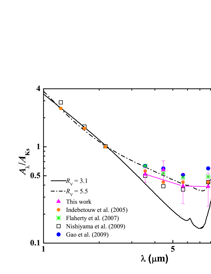
Figure 9: Comparison of the mid-IR extinction $A_{\lambda}/A_{\rm K_{s}}$ averaged over the five selected regions with the previous determinations for other regions and the WD01 $R_{\rm V}=3.1,5.5$ model extinction. The error bars indicate the standard deviation of five regions for each band.

Finally, we obtain the mean mid-IR extinction for the Coalsack nebula by averaging over the five selected regions: $A_{[3.6]}/A_{\rm K_{s}}\approx 0.519\pm 0.093$, $A_{[4.5]}/A_{\rm K_{s}}\approx 0.574\pm 0.140$, $A_{[5.8]}/A_{\rm K_{s}}\approx 0.391\pm 0.134$, and $A_{[8.0]}/A_{\rm K_{s}}\approx 0.387\pm 0.146$. The results are tabulated in Table 3 and illustrated in Figure 9. Also shown in Figure 9 are the previous determinations for other lines of sight (e.g., Indebetouw et al. 2005, Flaherty et al. 2007, Nishiyama et al. 2009, GJL09). The mean mid-IR extinction derived here for the Coalsack nebula is flat and roughly resembles the WD01 $R_{\rm V}=5.5$ model extinction curve. The 4.5$\,{\rm\mu m}$ extinction excess is also outstanding in the mean mid-IR extinction curve.

5 Discussion

To examine the effects of dust size on the extinction, we calculate the UV/optical/IR extinction from a mixture of amorphous silicate and graphite. We assume the standard “MRN” power-law size distribution (Mathis et al. 1977) for both dust components: $dn/da=A\,n_{\rm H}\,a^{-3.5}$ for $a_{\min}<a<a_{\rm max}$, where $a$ is the spherical radius of the dust (we assume the dust to be spherical), $a_{\rm min}=50\,{\rm\AA}$ is the lower cutoff of the dust size, $a_{\rm max}$ is the upper cutoff, $n_{\rm H}$ is the number density of H nuclei, and $A$ is constant ($A_{\rm sil}=10^{-25.11}\,{\rm cm}^{2.5}\,{\rm H}^{-1}$ for the silicate component, and $A_{\rm gra}=10^{-25.16}\,{\rm cm}^{2.5}\,{\rm H}^{-1}$ for the graphitic component; see Draine & Lee 1984). For the upper cutoff of the dust size, we take $a_{\rm max}=0.25,0.5,1,2.5\,{\rm\mu m}$. The $a_{\rm max}=0.25\,{\rm\mu m}$ case is known to closely reproduce the Galactic mean extinction curve of $R_{\rm V}=3.1$ (see Mathis et al. 1977, Draine & Lee 1984).

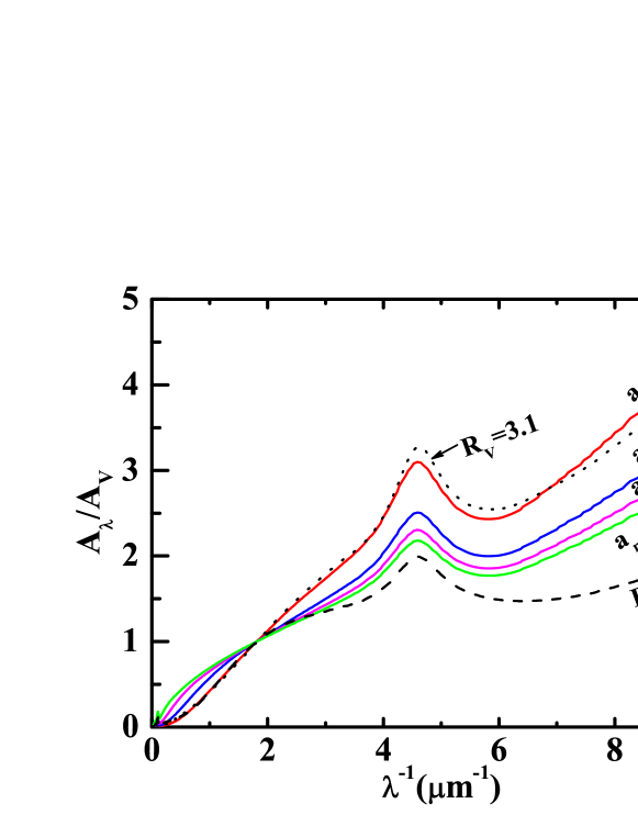
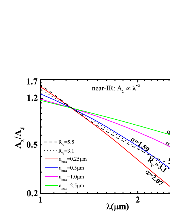
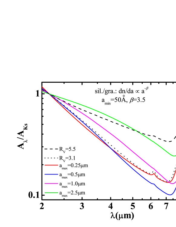
Figure 10: Upper panel (a): the UV/optical/near-IR extinction curves $A_{\lambda}/A_{\rm V}$ calculated from a mixture of amorphous silicate and graphite with a power-law size distribution $dn/da\propto a^{-3.5}$ with $a_{\rm min}=50\,{\rm\AA}$ and $a_{\rm max}=0.25\,{\rm\mu m}$ (red), $a_{\rm max}=0.5\,{\rm\mu m}$ (blue), $a_{\rm max}=1\,{\rm\mu m}$ (magenta), and $a_{\rm max}=2.5\,{\rm\mu m}$ (green). Also shown are the WD01 $R_{\rm V}=3.1$ (dotted) and $R_{\rm V}=5.5$ (dashed) model extinction curves. Middle panel (b): Same as (a) but for the near-IR extinction $A_{\lambda}/A_{\rm J}$. Lower panel (c): Same as (a) but for the mid-IR extinction $A_{\lambda}/A_{\rm K_{s}}$.

In Figure 10 we show the UV/optical, near-, and mid-IR extinction calculated from the dust mixture described above. It is apparent that the UV extinction $A_{\lambda}/A_{\rm V}$ flattens with the increase of dust size. The near-IR extinction $A_{\lambda}/A_{\rm J}$ also flattens with the increase of dust size: if we approximate the near-IR extinction as a power-law $A_{\lambda}\propto\lambda^{-\alpha}$, we would expect a smaller $\alpha$ from a larger $a_{\rm max}$. The variation of the mid-IR extinction $A_{\lambda}/A_{\rm K_{s}}$ with dust size is more complicated: unlike the UV and near-IR extinction, the mid-IR extinction does not monotonically flatten with the increase of $a_{\rm max}$, for example, $A_{\lambda}/A_{\rm K_{s}}$ steepens from $a_{\rm max}=0.25\,{\rm\mu m}$ to $a_{\rm max}=0.5\,{\rm\mu m}$, but it flattens again when increasing $a_{\rm max}$ to 1$\,{\rm\mu m}$ or larger (see Figure 10).

The fact that the mid-IR extinction curve of $a_{\rm max}=0.25\,{\rm\mu m}$ is even flatter than that of $a_{\rm max}=0.5\,{\rm\mu m}$ naturally explains the regional variations of the mid-IR extinction of the five regions selected in the Coalsack nebula: the “Diffuse” region has the lowest density and the smallest grain size and therefore the flattest mid-IR extinction; the other regions are denser and therefore their grain sizes are expected to be relatively larger and the resulting mid-IR extinction curves are steeper. This trend is also seen in the “CO–Strong” region and the “CO–Weak” region: the former is denser and its dust is larger and therefore its mid-IR extinction is relatively steeper.

However, it is puzzling that the mid-IR extinction of the “AV–Large” region is flatter than that of the “AV–Trans” region (and that of the “CO–Strong” region). One would think that the “AV–Large” region is denser than the “AV–Trans” region and its dust should be larger and therefore the mid-IR extinction should be steeper.

The “AV–Large” region contains Globule 2, the densest core in the Coalsack nebula. Bok et al. (1977) investigated this region based on the method of star counts and found $A_{\rm V}$ can reach $\,{\sim}$20 mag toward the center. The direction of the globule region has no known IRAS sources (Nyman et al., 1989; Bourke et al., 1995; Kato et al., 1999), protostellar objects or young clusters (Jones et al., 1980). The lack of YSOs indicates that this region has little star-forming activity.

Racca et al. (2002) used a polytropic model to describe the internal structure of this cloud, and argued that Globule 2 may be moderately unstable. Beuther et al. (2011) investigated the dynamical properties of the gas in Globule 2 with the APEX telescope through ¹³CO(2–1) which suggests that this region exists dynamical action (e.g., early infall activity). Hence, this cloud may be a young molecular cloud complex and not yet centrally condensed. The large $A_{\rm V}$ may then be caused by the sightline crossing long distance instead of large volume density of the dust. Indeed, Smith et al. (2002) argued that the diffuse components may contribute $A_{\rm V}\sim 5\,{\rm mag}$ to that of dense clouds in the Coalsack globules.

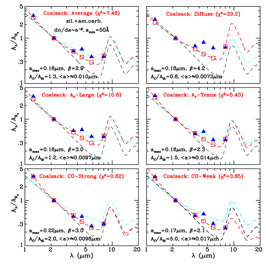
Figure 11: Comparison of the model extinction curve (red dashed line and red unfilled squares) with the IR extinction in the 2MASS and IRAC bands derived for the selected five regions of the Coalsack nebula as well as their mean values (blue filled triangles). The dust model consists of a mixture of amorphous silicate and amorphous carbon with an identical power-law size distribution for both dust components: $dn/da=A\,n_{\rm H}\,a^{-\beta}$ for $a_{\rm min}<a<a_{\rm max}$. With $a_{\rm min}=50\,{\rm\AA}$ fixed, $a_{\rm max}$, $\beta$, and $A_{\rm C}/A_{\rm Si}$ (the volume ratio of amorphous carbon to silicate) are treated as free parameters. The goodness of the fit is measured by $\chi^{2}\equiv\sum\left\{\left(A_{\lambda}/A_{\rm K_{s}}\right)_{\rm mod}-\left(A_{\lambda}/A_{\rm K_{s}}\right)_{\rm obs}\right\}^{2}/\left\{\Delta\left(A_{\lambda}/A_{\rm K_{s}}\right)\right\}^{2}$ where $\left(A_{\lambda}/A_{\rm K_{s}}\right)_{\rm mod}$ is the model extinction, $\left(A_{\lambda}/A_{\rm K_{s}}\right)_{\rm obs}$ and $\Delta\left(A_{\lambda}/A_{\rm K_{s}}\right)_{\rm obs}$ are the IR extinction and uncertainty at the 2MASS and IRAC bands derived for the selected regions. Also shown are the WD01 $R_{\rm V}=3.1$ (black dashed line) and $R_{\rm V}=5.5$ (cyan dot-dashed line) model extinction curves.

We stress that the above findings of steeper mid-IR extinction curves in denser regions are true only when the dust grains are small: as illustrated in Figure 10, the mid-IR extinction deepens from $a_{\rm max}=0.25\,{\rm\mu m}$ to $a_{\rm max}=0.5\,{\rm\mu m}$, while it flattens again from $a_{\rm max}=0.5\,{\rm\mu m}$ to $a_{\rm max}=1\,{\rm\mu m}$. To quantitatively examine this, we model the IR extinction curves in the 2MASS and IRAC bands derived for the selected five regions and their mean values in terms of a mixture of amorphous silicate and amorphous carbon. Both dust components are assumed to have the same size distribution $dn/da=A\,n_{\rm H}\,a^{-\beta}$ for $a_{\rm min}<a<a_{\rm max}$ with $a_{\rm min}=50\,{\rm\AA}$. The free parameters are $a_{\rm max}$, $\beta$, and the volume ratio of carbon dust to silicate dust $A_{\rm C}/A_{\rm Si}$. In Figure 11 we show the best-fit results for the selected five regions and their mean values. The model fits the derived extinction reasonably well except the IRAC [4.5] and [5.8] bands. The mean dust size $\langle a\rangle=\int_{a_{\rm min}}^{a_{\rm max}}a\,\left(dn/da\right)\,da/\int_{a_{\rm min}}^{a_{\rm max}}\left(dn/da\right)\,da$ is consistent with the flatness of the mid-IR extinction: the smaller $\langle a\rangle$ is, the flatter is the mid-IR extinction (e.g., the “AV–Large” region with $\langle a\rangle\approx 0.0097\,{\rm\mu m}$ has a flatter mid-IR extinction curve than that of the “AV–Trans” region for which $\langle a\rangle\approx 0.014\,{\rm\mu m}$). The mean dust size $\langle a\rangle$ is the smallest for the “Diffuse” region which has the flattest mid-IR extinction. The fact that the mid-IR extinction curve steepens with the increase of $\langle a\rangle$ indicates that the dust in the five regions in the Coalsack nebula is small: the dust has not yet grown sufficiently to the level that the mid-IR extinction flattens with the increase of $\langle a\rangle$ (see Figure 10). This suggests that the chemical evolution of the Coalsack nebula may be at too early a stage for the dust to significantly grow.

The extinction in the IRAC 4.5$\,{\rm\mu m}$ band, $A_{[4.5]}/A_{\rm K_{s}}$, is significantly higher than that of the other three IRAC bands (see Figure 8) and stands well above the model curve for all regions (see Figure 11). The 4.5$\,{\rm\mu m}$ extinction “excess” is particularly prominent for the “Diffuse” region. As clearly seen in Figure 9 and Table 3, the mean extinction of $A_{[4.5]}/A_{\rm K_{s}}\approx 0.574$ exceeds that of most of the other regions previously determined by others, and is comparable to the Galactic plane average of $A_{[4.5]}/A_{\rm K_{s}}\approx 0.57$ derived by GJL09. The detection of the 4.5$\,{\rm\mu m}$ extinction excess has also been reported in the LMC (see Gao et al. 2013).

Could the 4.5$\,{\rm\mu m}$ extinction “excess” arise from interstellar CO and CO₂ ices? CO ice has an absorption feature at 4.67$\,{\rm\mu m}$ due to the C–O stretch, while CO₂ ice has an absorption feature at 4.27$\,{\rm\mu m}$. These absorption features could contribute to the IRAC 4.5$\,{\rm\mu m}$ extinction. If CO and CO₂ ices are present, one would expect H₂O ice to be present as well, with an abundance usually much higher than that of CO and CO₂ ices (Whittet 2003, Gibb et al. 2004, Boogert et al. 2011). H₂O ice has two strong absorption bands: the O–H stretching feature at 3.05$\,{\rm\mu m}$ and the H–O–H bending feature at 6.02$\,{\rm\mu m}$.

To examine whether the ice (particularly CO₂ and, to a less degree, CO) absorption bands could account for the 4.5$\,{\rm\mu m}$ excess extinction, we approximate the 3.05, 4.27, 4.67 and 6.02$\,{\rm\mu m}$ bands respectively from H₂O, CO₂, CO, and H₂O ices as four Drude profiles. The extinction due to these four ice bands is

$$A_{\lambda}({\rm ice})=1.086\,N_{\rm H_{2}O}\sum\limits_{j=1}^{4}\frac{A_{j}\times\left[{\rm X}_{j}/{\rm H_{2}O}\right]\times E_{j}\times 2\gamma_{j}/\pi}{\left(\lambda-\lambda_{j}^{2}/\lambda\right)^{2}+\gamma_{j}^{2}}$$ (3)

where $\lambda_{j}$, $\gamma_{j}$, $A_{j}$ are the peak wavelength, FWHM, and strength of the $j$-th ice absorption band, respectively (see Table 4); $N_{\rm H_{2}O}$ is the H₂O ice column density; ${\rm X}_{j}/{\rm H_{2}O}$ is the abundance of the ice species ${\rm X}_{j}$ relative to H₂O ice in typical dense clouds; $E_{j}$ is the “enhancement” factor for species ${\rm X}_{j}$ (i.e., ${\rm X}_{j}/{\rm H_{2}O}$ is increased by a factor of $E_{j}$ in order for the ice absorption bands to account for the 4.5$\,{\rm\mu m}$ excess extinction). Finally, we add $\left(A_{\lambda}/A_{\rm K_{s}}\right)_{\rm ice}$, the ice extinction $A_{\lambda}({\rm ice})$ normalized to $A_{\rm K_{s}}({\rm ice})$, the ice extinction at the ${\rm K_{s}}$ band, to $\left(A_{\lambda}/A_{{\rm K_{s}}}\right)_{\rm WD}$, the WD01 model extinction curve (with $R_{\rm V}=3.1$),

$$A_{\lambda}/A_{\rm K_{s}}=\left(1-f_{\rm ice}\right)\times\left(A_{\lambda}/A_{{\rm K_{s}}}\right)_{\rm WD}+f_{\rm ice}\times\left(A_{\lambda}/A_{\rm K_{s}}\right)_{\rm ice}~{}~{},$$ (4)

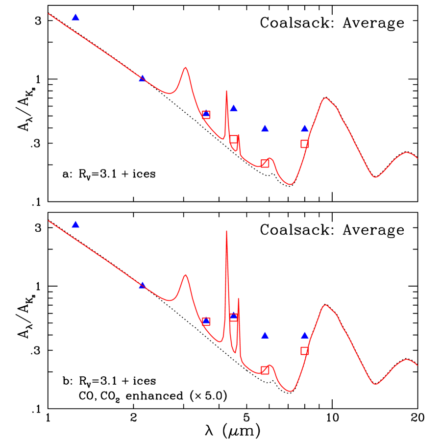
Figure 12: Comparison of the average extinction derived for the five selected regions of the Coalsack nebula (blue filled triangles) with the $R_{\rm V}=3.1$ model extinction curve (black dotted line) combined with the 3.05 and 6.02$\,{\rm\mu m}$ absorption bands of H₂O ice, the 4.27$\,{\rm\mu m}$ band of CO₂ ice, and the 4.67$\,{\rm\mu m}$ band of CO ice (red solid line). Open red squares are the $R_{\rm V}=3.1$ model curve plus the ice absorption bands convolved with the Spitzer/IRAC filter functions. The little bump at 6.2$\,{\rm\mu m}$ in the $R_{\rm V}=3.1$ model curve (black dotted line) is due to the C–C stretching absorption feature of polycyclic aromatic hydrocarbon (PAH) material (see Li & Draine 2001). Upper panel: the abundances of CO and CO₂ ices are taken to be that of typical dense clouds (i.e., ${\rm CO/H_{2}O=0.25}$, ${\rm CO_{2}/H_{2}O=0.21}$). Bottom panel: the abundances of CO and CO₂ ices are enhanced by a factor of five relative to their typical values in dense clouds.

where $f_{\rm ice}$ is the fractional amount of extinction at the ${\rm K_{s}}$ band contributed by ices. We then convolve $A_{\lambda}/A_{\rm K_{s}}$ with the Spitzer/IRAC filter response functions and, for demonstrative purposes, compare with the average mid-IR extinction derived for the Coalsack nebula (see Figure 12).

The H₂O ice quantity (i.e., $f_{\rm ice}$) is constrained not to exceed the IRAC 3.6$\,{\rm\mu m}$ extinction. With ${\rm CO/H_{2}O\approx 0.25}$ and ${\rm CO_{2}/H_{2}O\approx 0.21}$, typical for quiescent dense clouds (Whittet 2003, Gibb et al. 2004, Boogert et al. 2011), as shown in Figure 12a, CO and CO₂ are not capable of accounting for the 4.5$\,{\rm\mu m}$ excess extinction. If we are forced to attribute the 4.5$\,{\rm\mu m}$ excess extinction to CO and CO₂, we will have too much H₂O ice and the resulting extinction at 3.6$\,{\rm\mu m}$ would be too high. If we fix the H₂O ice abundance at what is required by the 3.6$\,{\rm\mu m}$ extinction, in order for CO and CO₂ to explain the 4.5$\,{\rm\mu m}$ excess extinction, we have to enhance their abundances (relative to their typical abundances in dense clouds) by a factor of $E_{\rm CO}=E_{\rm CO_{2}}\approx 5$ for $R_{\rm V}=3.1$ (see Figure 12b). The required CO and CO₂ abundances are unrealistically too high: ${\rm CO/H_{2}O\approx 1.3}$ and ${\rm CO_{2}/H_{2}O\approx 1.1}$. Also, the model still could not account for the flat extinction at 5.8$\,{\rm\mu m}$ and 8.0$\,{\rm\mu m}$ (see Figure 12b).

The 3.1$\,{\rm\mu m}$ H₂O ice absorption band has been detected in the Coalsack nebula. Smith et al. (2002) observed the lines of sight toward eight field stars lying behind three of the densest globules in the Coalsack nebula (i.e., Globules 1, 2, and 3) with the CTIO 4 m telescope and its IR spectrometer. They reported the detection of strong ice absorption in two sources (SS1-2 in Globule 1 and D7 in Globule 2), moderate or weak ice absorption in five sources (D4, D11, E9, and E18 in Globule 2, and SS3-1 in Globule 3), and very weak or no ice absorption in one source (E2 in Globule 2). The sightlines toward these stars are ideal for investigating the regional variations of the mid-IR extinction and particularly for examining the nature of the IRAC 4.5$\,{\rm\mu m}$ extinction excess. The optical depth of the 3.1$\,{\rm\mu m}$ ice absorption feature $\tau_{\rm ice}$ probes well whether a region is dense or diffuse: it is only seen in dense clouds and it is generally true that the higher $\tau_{\rm ice}$ is, the denser is the cloud. If the IRAC 4.5$\,{\rm\mu m}$ extinction excess is caused by CO and CO₂ ices, it should be more prominent in sightlines with strong ice absorption (e.g., D7 in Globule 2) and much less prominent or even disappear in sightlines with very weak or no ice absorption (e.g., E2 in Globule 2)

We use the “color-excess” method (see §3.1) and take RG stars as tracers to derive the mid-IR extinction in the IRAC bands for the six Globule 2 sightlines studied by Smith et al. (2002). In order to have enough sources (for each sightline) which can be used to derive extinction statistically, we consider an area of $4.8^{\prime}\times 4.2^{\prime}$ centered around each given star. As D4 and D11 are very close and their ice absorption strengths are comparable, we combine them into one region (hereafter “D4/D11”). The region that contains E9 is not considered since it overlaps parts of E2 and E18 and is difficult to separate it from them. Therefore, we have four regions for IR extinction studies: E2 – very weak ice absorption ($\tau_{\rm ice}\approx 0.01\pm 0.003$), E18 – moderate or weak ice absorption ($\tau_{\rm ice}\approx 0.07\pm 0.004$), D4/D11 – moderate or weak ice absorption ($\tau_{\rm ice}\approx 0.08\pm 0.004$), and D7 – strong ice absorption ($\tau_{\rm ice}\approx 0.34\pm 0.007$). The parameters (including the number of RG stars) of these regions are tabulated in Table 5. In Table 6 we tabulate the near-IR extinction power exponent $\alpha$ derived from the 2MASS photometry and the extinction ratio $A_{\lambda}/A_{\rm K_{s}}$ in the four IRAC bands.

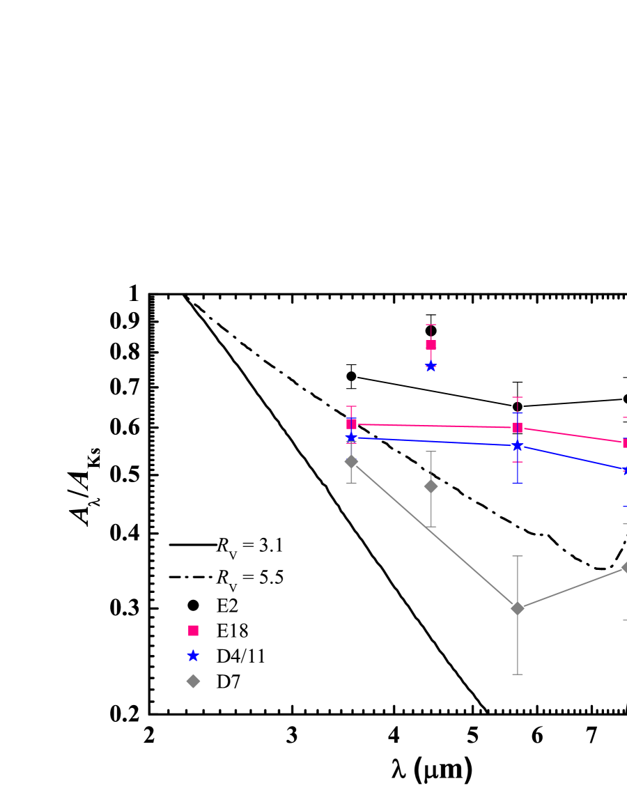
Figure 13: $A_{\lambda}/A_{\rm K_{s}}$ in the four IRAC bands of the four representative regions in the Coalsack nebula Globule 2 spanning a range of ice absorption strengths: D7 – strong ice absorption, D4/D11 and E18 – moderate or weak ice absorption, and E2 – very weak or no ice absorption. For comparison, the WD01 $R_{\rm V}=3.1,5.5$ model extinction curves are also shown.

The results are illustrated in Figure 13. It is apparent that $A_{\lambda}/A_{\rm K_{s}}$ in the IRAC bands increases with the decrease of $\tau_{\rm ice}$. This is consistent with our results for the “Diffuse”, “AV–Large”, “AV–Trans”, “CO–Strong” and “CO–Weak” regions: the mid-IR extinction curve flattens in less dense regions (provided that the dust is small), suggesting that the dust in the Coalsack nebula has not grown sufficiently even in the dense cloud sightline. Smith et al. (2002) found that in the Coalsack nebula, above a threshold of $A_{\rm V}\sim 7.6\,{\rm mag}$, the 3.1$\,{\rm\mu m}$ H₂O absorption optical depth $\tau_{\rm ice}$ correlates with the visual extinction $A_{\rm V}$: $\tau_{\rm ice}\approx 0.059\,\left(A_{\rm V}-7.6\right)$. Such a correlation is also seen in the Taurus dark cloud (a quiescent molecular cloud free from embedded young high mass stars) but with a smaller $A_{\rm V}$ threshold: $\tau_{\rm ice}\approx 0.059\,\left(A_{\rm V}-2.6\right)$ (Whittet et al. 1988b, Smith et al. 1993, Whittet et al. 2001). Smith et al. (2002) argued that there may exist a diffuse component contributing $A_{\rm V}\sim 5\,{\rm mag}$ to the extinction of the dense globules. Therefore, even the total visual extinction $A_{\rm V}$ is large toward a sightline, it may not necessarily be very dense (it might just be a pile-up of a long column of diffuse material). This also explains why the “AV–Large” region has a flatter mid-IR extinction curve than the “AV–Trans” region. This also explains why the dust in the Coalsack nebula has not grown effectively, just like that the ice mantles have not been effectively built up on grains.

We note that IRAC 4.5$\,{\rm\mu m}$ extinction excess is prominent in E2, the sightline with very weak or no ice absorption. On the other hand, although the 4.5$\,{\rm\mu m}$ extinction excess is also seen in D7 – the sightline with strong ice absorption, it is much weaker. No detection of the 4.27$\,{\rm\mu m}$ CO₂ ice feature or the 4.67$\,{\rm\mu m}$ CO ice feature was reported. Therefore, the 4.5$\,{\rm\mu m}$ extinction excess cannot be attributed to CO and CO₂ ices.

The origin of the 4.5$\,{\rm\mu m}$ excess extinction remains unknown. Some red giants have circumstellar envelopes rich in CO gas which absorbs at 4.6$\,{\rm\mu m}$(Bernat, 1981). With red giants as a tracer of the mid-IR extinction, the 4.6$\,{\rm\mu m}$ absorption feature of their CO gas could result in an overestimation of the IRAC 4.5$\,{\rm\mu m}$ extinction. It is worth exploring whether the CO gas absorption of red giants could account for the 4.5$\,{\rm\mu m}$ excess extinction.

6 Summary

Using data from the near-IR 2MASS Survey and the mid-IR Spitzer/GLIPMSE Legacy Program, we have derived the mid-IR extinction curves of five regions in the starless Coalsack nebula, spanning a range of interstellar environments from diffuse through translucent to dense clouds. The (relative) extinction $A_{\lambda}/A_{\rm K_{s}}$ in the four Spitzer/IRAC bands ([3.6], [4.5], [5.8], [8.0]$\,{\rm\mu m}$) are determined using the color-excess method and taking red giants as tracers. It is found that:

1. The mid-IR extinction curve exhibits appreciable regional variations. The extinction ratios $A_{\lambda}/A_{\rm K_{s}}$ in the IRAC bands are higher in diffuse regions than in denser regions. These variations can be explained in terms of dust size effects: the dust in dense regions is larger than that in diffuse regions, provided that the dust is small (i.e., it has not yet grown effectively in the Coalsack nebula).

2. The mean mid-IR extinction curve, with $A_{[3.6]}/A_{\rm K_{s}}\approx 0.519$, $A_{[4.5]}/A_{\rm K_{s}}\approx 0.574$, $A_{[5.8]}/A_{\rm K_{s}}\approx 0.391$, and $A_{[8.0]}/A_{\rm K_{s}}\approx 0.387$, is flat and consistent with previous results for various regions and the WD01 model extinction curve of $R_{\rm V}=5.5$.

3. The extinction in the IRAC 4.5$\,{\rm\mu m}$ band is much higher than that of the other three IRAC bands. It cannot be explained in terms of the 4.27$\,{\rm\mu m}$ absorption band of $\rm CO_{2}$ ice and the 4.67$\,{\rm\mu m}$ absorption band of CO ice. It may be caused by the 4.6$\,{\rm\mu m}$ absorption feature of CO gas in the circumstellar envelopes of some red giants.

4. The mid-IR extinction in the four IRAC bands have also been derived for four regions in the Coalsack Globule 2 which respectively exhibit strong ice absorption, moderate or weak ice absorption, and very weak or no ice absorption. The derived mid-IR extinction curves are all flat, with $A_{\lambda}/A_{\rm K_{s}}$ (in the IRAC bands) increasing with the decrease of the 3.1$\,{\rm\mu m}$ H₂O ice absorption optical depth $\tau_{\rm ice}$.

Figure 4: Antenna temperature $T_{\rm A}$ vs. the CO velocity $V_{\rm LSR}$ along the lines of sight toward the five selected regions in the Coalsack nebula. The name and coordinate of each region are labelled. For the “CO–Strong” region, two diagrams are shown, corresponding to two close regions which have the same galactic longitude but different galactic latitude. The CO data are taken from Nyman et al. (1989).

Table 1: Five regions in the Coalsack nebula selected for the IR extinction studies.

Selected	$l$	$b$	Area	Number of
Region	(deg)	(deg)	Covered	Sources
Diffuse	306.45	-0.85	$18^{\prime}\times 6^{\prime}$	245
AV–Large	300.75	-0.95	$30^{\prime}\times 12^{\prime}$	951
AV–Trans	300.75	-0.35	$30^{\prime}\times 12^{\prime}$	800
CO–Strong	303.40	-0.30	$36^{\prime}\times 24^{\prime}$	2769
CO–Weak	303.38	-0.96	$30^{\prime}\times 10.5^{\prime}$	657

Table 2: The 2MASS and Spitzer/IRAC color excess ratios for the five selected regions and their average values.

Region	$E_{{\rm J}-{\rm H}}/E_{{\rm H}-{\rm K_{s}}}$	$E_{{\rm K_{s}}-[3.6]}/E_{{\rm J}-{\rm K_{s}}}$	$E_{{\rm K_{s}}-[4.5]}/E_{{\rm J}-{\rm K_{s}}}$	$E_{{\rm K_{s}}-[5.8]}/E_{{\rm J}-{\rm K_{s}}}$	$E_{{\rm K_{s}}-[8.0]}/E_{{\rm J}-{\rm K_{s}}}$
Diffuse	1.680$\pm$0.062	0.216$\pm$0.018	0.125$\pm$0.028	0.251$\pm$0.024	0.241$\pm$0.023
AV–Large	1.876$\pm$0.019	0.203$\pm$0.004	0.188$\pm$0.007	0.265$\pm$0.006	0.269$\pm$0.006
AV–Trans	1.908$\pm$0.024	0.226$\pm$0.005	0.203$\pm$0.008	0.283$\pm$0.008	0.283$\pm$0.008
CO–Strong	1.928$\pm$0.009	0.237$\pm$0.002	0.236$\pm$0.003	0.308$\pm$0.003	0.294$\pm$0.003
CO–Weak	1.909$\pm$0.025	0.237$\pm$0.006	0.218$\pm$0.011	0.301$\pm$0.009	0.328$\pm$0.010
Mean	1.860$\pm$0.010	0.224$\pm$0.015	0.194$\pm$0.043	0.282$\pm$0.024	0.283$\pm$0.032

Table 3: IR extinction (relative to the 2MASS ${\rm K_{s}}$ band extinction) of the five selected regions in the Coalsack nebula.

Region	$\alpha$	$A_{\rm J}/A_{\rm K_{s}}$	$A_{[3.6]}/A_{\rm K_{s}}$	$A_{[4.5]}/A_{\rm K_{s}}$	$A_{[5.8]}/A_{\rm K_{s}}$	$A_{[8.0]}/A_{\rm K_{s}}$
Diffuse	1.73$\pm$0.01	2.56$\pm$0.01	0.665$\pm$0.028	0.806$\pm$0.043	0.609$\pm$0.038	0.625$\pm$0.035
AV–Large	2.14$\pm$0.01	3.19$\pm$0.01	0.556$\pm$0.009	0.587$\pm$0.016	0.418$\pm$0.014	0.410$\pm$0.013
AV–Trans	2.20$\pm$0.01	3.28$\pm$0.01	0.481$\pm$0.011	0.534$\pm$0.019	0.351$\pm$0.018	0.351$\pm$0.018
CO–Strong	2.24$\pm$0.01	3.37$\pm$0.01	0.439$\pm$0.004	0.441$\pm$0.008	0.270$\pm$0.007	0.304$\pm$0.007
CO–Weak	2.20$\pm$0.01	3.28$\pm$0.01	0.456$\pm$0.013	0.500$\pm$0.025	0.308$\pm$0.021	0.246$\pm$0.023
Mean	2.10$\pm$0.21	3.14$\pm$0.33	0.519$\pm$0.093	0.574$\pm$0.140	0.391$\pm$0.134	0.387$\pm$0.146

Table 4: Parameters for the four ice bands of H₂O, CO and CO₂ which may contribute to the mid-IR extinction in the Spitzer/IRAC bands.

Band	$\lambda_{j}$	Ice Species	FWHM	Band Strength	Abundance	Enhancement	$f_{\rm ice}$
$j$	($\mu$m)	${\rm X}_{j}$	$\gamma_{j}$ (cm-1)	$A_{j}$ (cm mol-1)	${\rm X}_{j}/{\rm H_{2}O}$	$E_{j}$ ($R_{\rm V}=3.1$)
1	3.05	H2O	335	$2.0\times 10^{-16}$	1	1	0.015
2	4.27	CO2	18	$7.6\times 10^{-17}$	0.21	5	0.015
3	4.67	CO	9.7	$1.1\times 10^{-17}$	0.25	5	0.015
4	6.02	H2O	160	$8.4\times 10^{-16}$	1	1	0.015

Table 5: Four representative lines of sight toward E2, E18, D4/D11, and D7 in the Coalsack Globule 2 which span a range of ice absorption strengths.

Name	Water Ice	$\tau_{\rm ice}$	$l$	$b$	Area	Number of
	Absorption		(deg)	(deg)	Covered	Sources
E2	Very Weak	0.01$\pm$0.03	300.65	-0.835	$4.8^{\prime}\times 4.2^{\prime}$	43
E18	Moderate/Weak	0.07$\pm$0.03	300.76	-0.775	$4.8^{\prime}\times 4.2^{\prime}$	61
D4/D11	Moderate/Weak	0.08$\pm$0.04	300.69	-0.905	$4.8^{\prime}\times 4.2^{\prime}$	50
D7	Strong	0.34$\pm$0.07	300.71	-0.975	$4.8^{\prime}\times 4.2^{\prime}$	46

Table 6: IR extinction (relative to the 2MASS ${\rm K_{s}}$ band extinction) of the regions in the Coalsack Globule 2 which span a range of ice absorption strengths.

Name	Ice Absorption	$\alpha$	$A_{[3.6]}/A_{\rm K_{s}}$	$A_{[4.5]}/A_{\rm K_{s}}$	$A_{[5.8]}/A_{\rm K_{s}}$	$A_{[8.0]}/A_{\rm K_{s}}$
E2	Very Weak	1.72$\pm$0.01	0.730$\pm$0.033	0.869$\pm$0.055	0.650$\pm$0.064	0.670$\pm$0.057
E18	Moderate/Weak	1.91$\pm$0.01	0.608$\pm$0.043	0.824$\pm$0.066	0.600$\pm$0.074	0.566$\pm$0.058
D4/D11	Moderate/Weak	2.14$\pm$0.01	0.577$\pm$0.045	0.759$\pm$0.077	0.560$\pm$0.075	0.510$\pm$0.066
D7	Strong	2.16$\pm$0.01	0.527$\pm$0.042	0.479$\pm$0.069	0.300$\pm$0.067	0.351$\pm$0.064

References

- Allen et al. (2004) Allen, L. E., et al. 2004, ApJS, 154, 363
- Ascenso et al. (2013) Ascenso, J., Lada, C. J., et al. 2013, A&A, 549, 135
- Benjamin et al. (2003) Benjamin, R. A., et al. 2003, PASP, 115, 953
- Bernat (1981) Bernat, A. P. 1981, ApJ, 246, 184
- Bertelli et al. (1994) Bertelli, G., Bressan, A., et al. 1994, A&AS, 106, 275
- Bertelli et al. (1999) Bertoldi, F., Timmermann, R., Rosenthal, D., Dropatz, S., et al. 1999, A&A, 346, 267
- Bessell & Brett (1988) Bessell, M. S., Brett, J. M., 1988, PASP, 100, 1134
- Beuther et al. (2011) Beuther, H., Kainulainen, J., Henning, Th., et al. 2011, A&A, 533, A17
- Bok et al. (1977) Bok, B. J., Sim, M. E., & Hawarden, T. G. 1977, Nature, 266, 145
- Boogert et al. (2011) Boogert, A. C. A., Huard, T. L., Cook, A. M., et al. 2011, ApJ, 729, 92
- Bourke et al. (1995) Bourke, T. L., Hyland, A. R., & Robinson, G. 1995, MNRAS, 276, 1052
- Cambrésy et al. (2011) Cambrésy, L. 1999, A&A, 345, 965
- Cambrésy et al. (2011) Cambrésy, L., Rho, J., Marshall, D. J., & Reach, W. T. 2011, A&A, 527, A141
- Cardelli et al. (1989) Cardelli, J. A.,Glayton, G. C., Mathis, J. S. 1989, ApJ, 345, 245
- Chapman et al. (2009) Chapman, N. L., Mundy, L. G., Lai, S.-P., et al. 2009, ApJ, 690,496
- Chrysostomou et al. (1996) Chrysostomou, A., Hough, J. H., Whittet, D. C. B., et al. 1996, ApJ. Lett. 465, L61
- Churchwell et al. (2009) Churchwell, E., et al. 2009, PASP, 121, 213
- Clark & Porter (2004) Clark J. S., Porter J. M., 2004, A&A, 427, 839
- Cutri et al. (2003) Cutri, R. M., et al. 2003, The IRSA 2MASS All-Sky Point Source Catalog NASA/IPAC Infrared Science Archive (Pasadena, CA: CalTech), http://irsa.ipac.caltech.edu/applications/Gator/
- Draine & Lee (1984) Draine, B. T., Lee, H. M., 1984, ApJ, 285, 89
- Draine (1989) Draine, B. T. 1989, in Infrared Spectroscopy in Astronomy, ed. B. H. Kaldeich (Paris: ESA Publications Division), 93
- Draine (2003) Draine, B. T. 2003, ARA&A, 41, 241
- Dobashi et al. (2005) Dobashi, K., Uehara, H., et al. 2005, PASJ, 57, S1
- Falco et al. (1999) Falco, E. E., Impey, C. D., Kochanek, C. S., et al. 1999, ApJ, 523, 617
- Flaherty et al. (2007) Flaherty, K., Pipher, J., Megeath, S., et al. 2007, ApJ, 663, 1069
- Fritz et al. (2011) Fritz, T. K., Gillessen, S., et al. 2011, ApJ, 737, 73
- Frogel et al. (1978) Frogel J. A., Persson S. E., Aaronson M., & Matthews K., 1978, ApJ, 220, 75
- Gao et al. (2009) Gao, J., Jiang, B. W., Li, A. 2009, ApJ, 707, 89 (GJL09)
- Gao et al. (2013) Gao, J., Jiang, B. W., Li, A., & Xue, M.Y. 2013, ApJ, submitted
- Gerakines et al. (1995) Gerakines, P. A., Schutte, W. A., et al. 1995, A&A, 296, 810
- Gibb et al. (2004) Gibb, E. L., Whittet, D. C. B., et al. 2004, ApJS, 151, 35
- Glass et al. (1999) Glass, I., et al. 1999, MNRAS, 308, 127
- Gómez & Kenyon (2001) Gómez, M., & Kenyon, S. J. 2001, AJ, 121, 974
- Gregorio-Hetem et al. (1988) Gegorio Hetem, J. C., Sanzovo, G. C., et al. 1988, A&AS, 76, 347
- He et al. (1995) He, L., Whittet, D. C. B., Kilkenny, D., & Spencer Jones, J. H. 1995, ApJS, 101, 335
- Indebetouw et al. (2005) Indebetouw, R., et al. 2005, ApJ, 619, 931
- Jiang et al. (2006) Jiang, B. W., Gao, J., Omont, A., Schuller, F., & Simon, G. 2006, A&A, 446, 551
- Jones et al. (1980) Jones, T. J., Hyland, A. R., Robinson, G., et al. 1980, ApJ, 242, 132
- Kainulainen et al. (2009) Kainulainen, J., Beuther, H., Henning, T., & Plume, R. 2009, A&A, 508, L35
- Kato et al. (1999) Kato, S., Mizuno, N., Asayama, S.CI., et al. 1999, PASJ, 51, 883
- Kenyon et al. (1998) Kenyon, S. J., Lada, E. A., & Barsony, M. 1998, AJ, 115, 252
- Li & Draine (2001) Li, A., & Draine, B. T. 2001, ApJ, 554, 778
- Lutz et al. (1996) Lutz, D., et al. 1996, A&A, 315, L269
- Magnani et al. (1985) Magnani, L., Blitz, L., & Mundy, L. 1985, ApJ, 295, 402
- Marengo et al. (2007) Marengo, M., Hora, J. L., Barmby, P., et al. 2007, in ASP Conf. Ser. 378, Why Galaxies Care About AGB Stars: Their Importance as Actors and Probes, ed. F. Kerschbaum, C. Charbonnel, & R. F. Wing (San Francisco CA: ASP), 80
- Marshall et al. (2006) Marshall, D. J., Robin, A. C., Reylé, C., et al. 2006, A&A, 453, 635
- Martin & Whittet (1990) Martin, P. G., Whittet, D. C. B. 1990, ApJ, 357, 113
- Mathis et al. (1977) Mathis, J. S., Rumpl, W., & Nordsieck, K. H. 1977, ApJ, 217, 425
- Mathis (1990) Mathis, J. S. 1990, ARA&A, 28, 37
- McClure (2009) McClure, M. 2009, ApJ, 693, L81
- Moore et al. (2005) Moore, T. J. T., Lumsden, S. L., Ridge, N. A., et al. 2005, MNRAS, 359, 589
- Naoi (2006) Naoi, T., Tamura, M., Nakajima, Y., et al. 2006, ApJ, 640, 373
- Naoi et al. (2007) Naoi, T., Tamura, M., Nagata, T., et al. 2007, ApJ, 658, 1114
- Nishiyama et al. (2009) Nishiyama, S., Tamura, M., Hatano, H., et al. 2009, ApJ, 696, 1407
- Nyman et al. (1989) Nyman, L. A., Bronfman, L., & Thaddeus, P. 1989, A&A, 216, 185
- Nyman (2008) Nyman, L. A. 2008, Handbook of Star Forming Regions, 2
- Racca et al. (2002) Racca, G., Gomez, M., & Kenyon, S. J. 2002, AJ, 124, 2178
- Román-Zúñiga et al. (2007) Román-Zúñiga, C. G., Lada, C. J., Muench, A., & Alves, J. F. 2007, ApJ, 664, 357
- Rosenthal et al. (2000) Rosenthal, D., Bertoldi, F., & Drapatz, S. 2000, A&A, 356, 705
- Rieke & Lebofsky (1985) Rieke, G. H., Lebofsky, M. J. 1985, ApJ, 288, 618
- Skrutskie et al. (2006) Skrutskie, M. F., et al. 2006, AJ, 131, 1163
- Smith et al. (1993) Smith, R. G., Sellgren, K., & Brooke, T. Y. 1993, MNRAS, 263, 749
- Smith et al. (2002) Smith, R. G., Blum, R. D., Quinn, D. E., et al. 2002, MNRAS, 330, 837
- Snow & McCall (2006) Snow, T. P., McCall, B. J. 2006, ARA&A, 44, 367
- Stead & HoareStead (2009) Stead, J. J., & Hoare, M. G. 2009, MNRAS, 400, 731
- Tapia (1973) Tapia, S. 1973, in IAU Symp. 52, Interstellar Dust and Related Topics, ed. J. M. Greenberg & H. C. van de Hulst (Dordrecht: Reidel), 43
- van Dishoeck (1994) van Dishoeck, E. F., 1994, in: The Infrared Cirrus and Diffuse Interstellar Clouds, Cutri, R. & Latters, W.B. (eds.), San Francisco, ASP Conference Series 58, p. 319
- Wainscoat et al. (1992) Wainscoat, R., Cohen, M., Volk, K., et al. 1992, ApJS, 83, 146
- Wang et al. (2004) Wang, J., Hall, P. B., Ge, J., Li, A., & Schneider, D. P. 2004, ApJ, 609, 589
- Weingartner & Draine (2001) Weingartner, J. C., & Draine, B. T. 2001, ApJ, 548, 296
- Whittet (1988a) Whittet, D. C. B. 1988a, Dust in the Universe, ed. M. E. Bailey & D. A. Williams (Cambridge: Cambridge Univ. Press), 25
- Whittet (1988b) Whittet, D. C. B., Bode, M. F., et al. 1988b, MNRAS, 233, 321
- Whittet et al. (2001) Whittet, D. C. B., Gerakines, P. A., Hough, J. H., & Shenoy, S. S. 2001, ApJ, 547, 872
- Whittet (2003) Whittet, D. C. B. 2003, Dust in the Galactic Environment (Bristol: Inst. Phys. Publ.), pp. 66
- Zasowski et al. (2009) Zasowski, G., Majewski, S. R., Indebetouw, R., et al. 2009, ApJ, 707, 510