Joint modelling of ChIP-seq data via a Markov random field model

Abstract: Chromatin ImmunoPrecipitation-sequencing (ChIP-seq) experiments have now become routine in biology for the detection of protein binding sites. In this paper, we present a Markov random field model for the joint analysis of multiple ChIP-seq experiments. The proposed model naturally accounts for spatial dependencies in the data, by assuming first order Markov properties, and for the large proportion of zero counts, by using zero-inflated mixture distributions. In contrast to all other available implementations, the model allows for the joint modelling of multiple experiments, by incorporating key aspects of the experimental design. In particular, the model uses the information about replicates and about the different antibodies used in the experiments. An extensive simulation study shows a lower false non-discovery rate for the proposed method, compared to existing methods, at the same false discovery rate. Finally, we present an analysis on real data for the detection of histone modifications of two chromatin modifiers from eight ChIP-seq experiments, including technical replicates with different IP efficiencies.

1 Introduction

ChIP-sequencing, also known as ChIP-seq, is a well-known biological technique to detect protein-DNA interactions, DNA methylation, and histone modifications in vivo. ChIP-seq combines Chromatin ImmunoPrecipitation (ChIP) with massively parallel DNA sequencing to identify all DNA binding sites of a transcription factor or genomic regions with certain histone modification marks. The final data produced by the experiment provide the number of DNA fragments in the sample aligned to each location of the genome. From this, the aim of the statistical analysis is to distinguish the truly enriched regions along the genome from the background noise. Whereas conventional transcription factors, that bind directly to the DNA, show sharp peaks at the regions of enrichment, chromatin modifiers tend to have much broader regions of enrichment and do not follow a peak-like pattern. The latter cannot be captured by standard peak-calling algorithms and require more sophisticated statistical models. This is the focus of the present paper.

As regions of the genome are either bound by the protein in question or not, it is quite common to analyse such data using a mixture model. Here the observed counts are assumed to come either from a signal or from a background distribution. A number of methods have adopted this approach, with some differences in the distribution chosen for the mixture. Spyrou et al. (2009), in their BayesPeak R package, adopt a Negative Binomial (NB) mixture model, with a NB distribution used both for signal and background. Kuan et al. (2011), in their MOSAiCS package, adopt a more flexible NB mixture model, where an offset is included in the signal distribution and this distribution itself is taken as a mixture of NBs. Spyrou et al. (2009) show evidence that a NB mixture model outperforms a Poisson mixture model, such as the one used by Iseq (Mo, 2012). Qin et al. (2010), in their HPeak implementation, suggest to use a zero-inflated Poisson model for the background and a generalized Poisson distribution for the signal. In this paper we consider a more flexible framework by allowing a zero-inflated Poisson or NB distribution for the background and a Poisson or NB distribution for the signal component.

Another feature of ChIP-seq data on histone modifications is the spatial dependency of counts for neighbouring windows along the genome. This is mainly the result of a common pre-processing step, whereby the genome is divided into bins of some ad-hoc length. It is quite common to consider fixed-width windows, although dynamic approaches have also been considered (Mo, 2012). The sum of counts within each window is subsequently considered for the analysis. As a result of this, true regions of the genome that are bound by the protein in question could be easily found to cross two or more pre-processed bins. This issue has been addressed in the literature with the use of Hidden Markov Models (HMMs) (Spyrou et al., 2009; Mo, 2012; Qin et al., 2010).

With few exceptions, the methods developed so far are limited to the analysis of single experiments, with the optional addition of a control experiment. When technical replicates or biological replicates are available, the standard procedure is to perform the peak calling on each individual data set and then combine the results by retaining the common regions. This process has inherent statistical problems, as pointed out by Bardet et al. (2012) and Bao et al. (2013). Despite the recognition of the need for biological replicates for ChIP-seq analyses (Tuteja et al., 2009) and despite the fact that several normalization methods have been proposed for multiple ChIP-seq experiments (Bardet et al., 2012; Shao et al., 2012), very few methods have been developed that combine technical and biological replicates at the modelling stage. This would allow to properly account for the variability in the data, leading to a more robust detection of enriched and differentially bound regions. Zeng et al. (2013) extend MOSAiCS (Kuan et al., 2011), by developing a mixture model for multiple ChIP-seq datasets: individual models are used to analyse counts for each experiment and a final model is considered to govern the relationship of enrichment among different samples. Bao et al. (2013) build mixture models for multiple experiments, where replicates are modelled jointly by an assumption of a shared latent binding profile. In Bao et al. (2013), we show how such a joint modelling approach leads to a more accurate detection of enriched and differentially bound regions and how it allows to account for the different IP efficiencies of individual ChIP-seq experiments. The latter has probably been the main reason why joint modelling approaches of ChIP-seq data have rarely been considered so far.

In this paper, we combine all the aspects described above into a single model, by proposing a one-dimensional Markov random field model for the analysis of multiple ChIP-seq data. Our model can be viewed as a hidden Markov model where the initial distribution is a stationary distribution. As such, we follow the existing literature on the use of hidden Markov models for ChIP-seq data in order to account for the spatial dependencies in the data (Spyrou et al., 2009; Mo, 2012). In contrast to the existing HMM-based methods, we propose a joint statistical model for ChIP-seq data, under general experimental designs. In particular, we discuss the case of technical and biological replicates as well as the case of different antibodies and/or IP efficiencies associated to each experiment. The remainder of this paper is organized as follows. In Section 2, we describe the Markov random field model and its Bayesian Markov Chain Monte Carlo (MCMC) implementation. In Section 3, we perform a simulation study to compare our method with two existing HMM-based methods, BayesPeak and iSeq, as well as with the joint mixture model of Bao et al. (2013). A real data analysis on eight experiments for the detection of histone modifications of two proteins, CBP and p300, is given in Section 4. In Section 5, we conclude with a brief discussion.

2 Methods

2.1 A joint latent mixture model and its limitations

The data generated by ChIP-sequencing experiments report the number of aligned DNA fragments in the sample for each position along the genome. Due to noise and the size of the genome, it is common to summarise the raw counts by dividing the genome into consecutive windows, or bins. Since the majority of the genome is expected to be not enriched, we would generally expect that some bins are enriched regions, with a lot of tags, and most other bins are not enriched, containing only few tags. This scenario is well suited to a mixture model framework.

Let $M$ be the total number of bins and $Y_{mcar}$ the counts in the $m$th bin, $m=1,2,\cdots,M$, under condition $c$, antibody $a$ and replicate $r$. In the ChIP-seq context, the condition $c$ stands for a particular protein and/or a particular time point, and $r=1,\ldots,R_{ca}$ is the number of replicates for antibody $a$ under condition $c$, with $a=1,\ldots,A$. It is well known how a different level of ChIP efficiency is associated to different antibodies and how different IP efficiencies have been observed also for technical replicates (Bao et al., 2013). The current setup allows to account for these effects in the joint statistical modelling of multiple ChIP-seq experiments, under a variety of common experimental designs. The counts $Y_{mcar}$ are either from a background population (non-enriched region) or a from a signal population (enriched region). Let $X_{mc}$ be the unobserved random variable specifying if the $m$th bin is enriched ($X_{mc}=1$) or non-enriched ($X_{mc}=0$) under condition $c$. Clearly, this latent state does not depend on ChIP efficiencies. As in Bao et al. (2013), we define a joint mixture model for $Y_{mcar}$ as follows:

$$Y_{mcar} \sim p_{c}f(y|\theta^{S}_{car})+(1-p_{c})f(y|\theta^{B}_{car}),$$

where $p_{c}=P(X_{mc}=1)$ is the mixture portion of the signal component and $f(y,\theta^{S}_{car})$ and $f(y,\theta^{B}_{car})$ are the signal and background densities for condition $c$, antibody $a$ and replicate $r$, respectively. Using this model, the regions are detected as enriched or not by controlling the False Discovery Rate (FDR).

Since we divide the genome arbitrarily in fixed-size windows, it is possible that a region in a certain cromatin state crosses two or more bins. As a consequence of this, it is reasonable to assume that the enriched regions have some Markov property. We have checked whether this is the case for ChIP-seq data from a real study, after dividing the genome into 200bp fixed windows. We have detected the enriched regions using the latent mixture model above at a $5\%$ FDR and then calculated the conditional frequencies for each region, given that the previous region is enriched or non enriched. We denote these by $f_{1|1}$ and $f_{1|0}$, respectively. Table 1 shows that these two frequencies are generally not equal. The conditional frequency of a current bin being enriched given that the previous bin is enriched is generally larger than the conditional frequency of a bin being enriched given that the previous bin is not enriched. As a further evidence of Markov properties, Figure 1 plots the bin counts $Y_{m}$ for a region of the genome, for one ChIP-seq experiment. On the right, the plot shows the posterior probability of enrichment, using a latent mixture model. This plot clearly shows regions of consecutive enriched bins.
TABLE 1 and FIGURE 1 ABOUT HERE.

The issue of spatial dependencies in ChIP-seq data is often overcome in the literature by repeating the experiments using some ad-hoc shift of regions, usually taken as half of the original window size. In this paper, we propose a natural extension of the mixture model in (2.1), which accounts for the spatial Markov properties of the data. This is described in the next section.

2.2 A one-dimensional Markov random field model

The number of reads in bin $m$, $Y_{m}$, is either drawn from a signal or a background distribution. To simplify the notation, we will omit the subscripts $c,a,r$ in this section. The first issue is about the choice of the mixture distribution. Together with the general expectation that a large part of the genome is not bound by the protein in question, unmapped genome regions and insufficient sequencing depth, i.e. an insufficient total number of reads, give rise to an excess of zeros in the observed data. This forms part of the background noise and gives us the motivation to use a zero-inflated distribution to model the background. As the data is in forms of counts, it is natural to consider either a Zero-Inflated Poisson (ZIP) or a Zero-Inflated Negative Binomial (ZINB) distribution. That is, conditional on the latent state $X_{m}$,

$$Y_{m}|X_{m}=0\sim{\rm ZIP}(\pi,\lambda_{0})\>{\rm or}\>{\rm ZINB}(\pi,\mu_{0},\phi_{0}),\>\>\>\>Y_{m}|X_{m}=1\sim{\rm Poisson}(\lambda_{1})\>{\rm or}\>{\rm NB}(\mu_{1},\phi_{1}),$$

where the probability density function of the zero-inflated Poisson is given by:

$$ZIP(y|\pi,\lambda)=\left\{\begin{array}[]{lr}(1-\pi)+\pi\exp(-\lambda)&\text{ if }y=0,\\ \\ \displaystyle\frac{\pi\exp(-\lambda)\lambda^{y}}{y!}&\text{ if }y>0.\end{array}\right.$$ (4)

and the probability density function of the zero-inflated negative binomial is given by:

$$ZINB(y|\pi,\mu,\phi)=\left\{\begin{array}[]{lr}(1-\pi)+\pi(\displaystyle\frac{\phi}{\mu+\phi})^{\phi}&\text{ if }y=0,\\ \\ \displaystyle\frac{\Gamma(y+\phi)}{\Gamma(\phi)\Gamma(y+1)}(\frac{\mu}{\mu+\phi})^{y}(\frac{\phi}{\mu+\phi})^{\phi}&\text{ if }y>0.\end{array}\right.$$ (8)

A zero-inflated model can be seen as a mixture model of a zero mass distribution and a Poisson/NB distribution, so it can be interpreted with the use of another latent variable which represents the extra zeros in the background regions that a standard Poisson/NB distribution cannot account for. If we denote this inner latent variable by $Z_{m}$ and $P(Z_{m}=1|X_{m}=0)=\pi$, then conditional on $X_{m}$, we have

$$Y_{m}|X_{m}=0,Z_{m}=0 \sim 1(y=0)$$

$$Y_{m}|X_{m}=0,Z_{m}=1 \sim {\rm Poisson}(\lambda_{0})\>{\rm or}\>{\rm NB}(\mu_{0},\phi_{0}),\>\>Y_{m}|X_{m}=1\sim{\rm Poisson}(\lambda_{1})\>{\rm or}\>{\rm NB}(\mu_{1},\phi_{1}).$$

The latent variable $X_{m}$, representing the binding profile, is assumed to satisfy one dimensional Markov properties, that is,

$$P(X_{m}=i|X_{-m})=P(X_{m}=i|X_{m-1},X_{m+1}),i\in\{0,1\}.$$ (9)

This give the classical factorization of the joint density

$$P(X_{1},X_{2},\ldots,X_{M}) = \pi_{0}(X_{1})\begin{tabular}[]{c}$\scriptstyle{M-1}$\\ $\displaystyle{\prod}$\\ $\scriptstyle{m=1}$\end{tabular}q_{X_{m},X_{m+1}}$$ (13)

in terms of the initial state distribution $\pi_{0}$ and transition probabilities $q_{i,j}=P(X_{m+1}=j|X_{m}=i),i,j\in\{0,1\}$. Unlike the model above, in this paper we use a more natural representation of the joint density of the latent states for a one-dimensional Markov random field model, namely:

$$P(X_{1},X_{2},\ldots,X_{M}) = \frac{\begin{tabular}[]{c}$\scriptstyle{M-1}$\\ $\displaystyle{\prod}$\\ $\scriptstyle{m=1}$\end{tabular}P(X_{m},X_{m+1})}{\begin{tabular}[]{c}$\scriptstyle{M-1}$\\ $\displaystyle{\prod}$\\ $\scriptstyle{m=2}$\end{tabular}P(X_{m})}$$ (20)

where $P(X_{m},X_{m+1})$ is the joint probability of $X_{m}$ and $X_{m+1}$ and $P(X_{m})$ is the marginal probability of $X_{m}$. In particular, we have $P(X_{m})=\displaystyle\sum_{x_{m+1}}P(X_{m},X_{m+1}=x_{m+1})$.

When the $X_{m}$ are binary variables, as in our case, we can further re-write the model (20) as

$$P(X_{1},X_{2},\ldots,X_{M})={\delta_{1}}^{I(X_{1}=1)}{\delta_{0}}^{I(X_{1}=0)}{\Big{(}\frac{\delta_{1,1}}{\delta_{1}}\Big{)}}^{n_{1,1}}{\Big{(}\frac{\delta_{1,0}}{\delta_{1}}\Big{)}}^{n_{1,0}}{\Big{(}\frac{\delta_{0,1}}{\delta_{0}}\Big{)}}^{n_{0,1}}{\Big{(}\frac{\delta_{0,0}}{\delta_{0}}\Big{)}}^{n_{0,0}},$$

where

$$n_{i,j} = \#\{X_{m}=i,X_{m+1}=j\},\>\>\delta_{i,j}=P(X_{m}=i,X_{m+1}=j),i,j\in\{0,1\},m=1,\ldots,M-1$$

$$\delta_{1} = P(X_{m}=1)=\delta_{1,1}+\delta_{1,0},\>\>\>\delta_{0}=P(X_{m}=0)=1-\delta_{1},\>\>\delta_{0,1}=\delta_{1,0}=(1-\delta_{1,1}-\delta_{0,0})/2.$$

One can show that this model satisfies (9), that is the model is a one-dimensional Markov random field model. And if we notice that the transition probabilities satisfy $q_{i,j}=\delta_{i,j}/\delta_{i}$, the model can be further written in terms of the transition probabilities $q_{i,j}$ as following

$$P(X_{1},X_{2},\ldots,X_{M}) = {\Big{(}\frac{q_{0,1}}{q_{0,1}+q_{1,0}}\Big{)}}^{I(X_{1}=1)}{\Big{(}\frac{q_{1,0}}{q_{0,1}+q_{1,0}}\Big{)}}^{I(X_{1}=0)}q_{1,1}^{n_{1,1}}q_{1,0}^{n_{1,0}}q_{0,1}^{n_{0,1}}q_{0,0}^{n_{0,0}}.$$ (21)

The most attractive property of this model is that the initial state distribution under (20) is the stationary distribution. This is different from BayesPeak (Spyrou et al., 2009). Note also that the Ising model of Mo (2012) has one parameter less than the model presented here: this corresponds to assuming that $q_{1,1}+q_{0,1}=1$, which is an unnecessary assumption and it is not normally satisfied by the data.

2.3 Parameter Estimation

To simplify the notation, we define $\tilde{q}_{1}=q_{1,1}$ and $\tilde{q}_{0}=q_{0,1}$. These are the probabilities that the current state of a bin is 1 (enriched) given that the state of the left bin is 1 and 0, respectively. We denote with $R_{c}$ the number of replicates under condition $c$. For simplicity, we drop the subscript $c$ in what follows and we assume that the same antibody is used for all replicates under a particular condition, which is often the case in practice. A similar derivation applies to the more general case as well as to the more specific case of no replicates. Assuming a ZINB-NB mixture model (zero-inflated NB for the background and NB for the signal), we aim to estimate the parameters $\Theta=(\tilde{q}_{0},\tilde{q}_{1},\pi,\mu_{0},\phi_{0},\mu_{1},\phi_{1})$. The joint likelihood of this model given the latent states, X, the inner variables $\textbf{Z}_{1},\ldots,\textbf{Z}_{R}$ and data $\textbf{Y}_{1},\ldots,\textbf{Y}_{R}$, is given by

$$P(\textbf{X},\textbf{Z},\textbf{Y}|\Theta) = P(\textbf{X}|\Theta)P(\textbf{Z}|\textbf{X}=0,\Theta)P(\textbf{Y}|\textbf{X},\textbf{Z},\Theta)$$ (25)

$$\propto {\Big{(}\frac{\tilde{q}_{0}}{\tilde{q}_{0}+1-\tilde{q}_{1}}\Big{)}}^{I(X_{1}=1)}{\Big{(}\frac{1-\tilde{q}_{1}}{\tilde{q}_{0}+1-\tilde{q}_{1}}\Big{)}}^{I(X_{1}=0)}\tilde{q}_{1}^{n_{1,1}}(1-\tilde{q}_{1})^{n_{1,0}}\tilde{q}_{0}^{n_{0,1}}(1-\tilde{q}_{0})^{n_{0,0}}$$

$$\times \begin{tabular}[]{c}$\scriptstyle{{R}}$\\ $\displaystyle{\prod}$\\ $\scriptstyle{r=1}$\end{tabular}\pi_{r}^{\Sigma_{m}I(X_{m}=0,Z_{mr}=1)}\times(1-\pi_{r})^{\Sigma_{m}I(X_{m}=0,Z_{mr}=0)}$$

$$\times \begin{tabular}[]{c}$\scriptstyle{R}$\\ $\displaystyle{\prod}$\\ $\scriptstyle{r=1}$\end{tabular}\begin{tabular}[]{c}$\scriptstyle{M}$\\ $\displaystyle{\prod}$\\ $\scriptstyle{m=1}$\end{tabular}\Big{[}\frac{\Gamma(y_{mr}+\phi_{0r})}{\Gamma(\phi_{0r})\Gamma(y_{mr}+1)}\Big{(}\frac{\mu_{0r}}{\mu_{0r}+\phi_{0r}}\Big{)}^{y_{mr}}\Big{(}\frac{\phi_{0r}}{\mu_{0r}+\phi_{0r}}\Big{)}^{\phi_{0r}}\Big{]}^{I[X_{m}=0,Z_{mr}=1]}$$ (32)

$$\times \begin{tabular}[]{c}$\scriptstyle{R}$\\ $\displaystyle{\prod}$\\ $\scriptstyle{r=1}$\end{tabular}\begin{tabular}[]{c}$\scriptstyle{M}$\\ $\displaystyle{\prod}$\\ $\scriptstyle{m=1}$\end{tabular}\Big{[}\frac{\Gamma(y_{mr}+\phi_{1r})}{\Gamma(\phi_{1r})\Gamma(y_{mr}+1)}\Big{(}\frac{\mu_{1r}}{\mu_{1r}+\phi_{1r}}\Big{)}^{y_{mr}}\Big{(}\frac{\phi_{1r}}{\mu_{1r}+\phi_{1r}}\Big{)}^{\phi_{1r}}\Big{]}^{I[X_{m}=1]}.$$ (39)

Here we assume that technical and biological replicates share the same binding profiles, i.e. the latent states $X$ are common between replicates. This results in the joint probabilities $P(X_{m},X_{m+1})$ in equation (20) being equal for all replicates, and consequently, the transition probabilities $\tilde{q}_{0}$ and $\tilde{q}_{1}$ in equation (21) are also equal across replicates. A similar derivation applies for the ZIP-Poisson mixture model (zero-inflated Poisson for the background and Poisson for the signal) for the estimation of the parameters $\Theta=(\tilde{q}_{0},\tilde{q}_{1},\pi,\lambda_{0},\lambda_{1})$.

We use a Bayesian methodology, in a Metropolis-within-Gibbs procedure, to estimate the model parameters and states. In particular, we use a Direct Gibbs (DG) method to draw the latent state $X$. DG treats each state as a separate parameter term and draws each $X_{m}$, for $m=1,\ldots,M$, from its full conditional distribution

$$P(X_{m}=i|X_{-m},\textbf{Y}_{1},\ldots,\textbf{Y}_{R},\Theta)\propto q_{X_{m-1},i}q_{i,X_{m+1}}\begin{tabular}[]{c}$\scriptstyle{R}$\\ $\displaystyle{\prod}$\\ $\scriptstyle{r=1}$\end{tabular}P_{i}(Y_{mr}|\Theta)$$

where $X_{-m}=\{X_{1},\ldots,X_{m-1},X_{m+1},\ldots,X_{M}\}$, $P_{i}(Y_{mr}|\Theta)=P(Y_{mr}|X_{m}=i,\Theta)$ and the normalising constant is the sum over all possible values of $i$. Given $X_{m}=0$, the inner latent variable $Z_{mr}$ is drawn from its full conditional distribution

$$P(Z_{mr}=i|X_{m}=0,Y_{mr}=y_{mr},\Theta)\propto P(y_{mr}|X_{m}=0,Z_{mr}=i,\Theta)P(Z_{mr}=i|X_{m}=0).$$

We choose Gamma and Beta conjugate priors for the parameters and draw samples from their posterior distributions. More details are given in the supplementary material.

2.4 Assuming the same number of binding sites across conditions

The method above can be used in the presence of technical and biological replicates. Whereas technical and biological replicates share the same binding profile X, different proteins will generally have a different binding profile. Under certain conditions, e.g. when comparing the binding profiles across two conditions or between highly similar transcription factors, we can assume that the total number of binding sites is the same. In Bao et al. (2013), we show how this assumption can be included in a mixture modelling framework. In this paper, we show how the same assumption can be included also in the proposed Markov random field mixture model.

In particular, if $\textbf{X}_{1}$ and $\textbf{X}_{2}$ are the binding profiles of conditions 1 and 2, respectively (e.g. protein 1 and protein 2), we can include in the joint model the a priori biological knowledge that the two conditions have the same number of binding sites, i.e. $P(X_{m1}=1)=P(X_{m2}=1)$ for any region $m$. If the transition probabilities $q$ are the same for the two conditions, then from our stationary random field model (21), the stationary distributions of the two experiments are also the same. However, assuming equal transition probabilities is quite a strong assumption and it is difficult to know this beforehand, unless we are in the presence of technical replicates. If we note that the stationary distribution $P(X=1)=\displaystyle\frac{\tilde{q}_{0}}{\tilde{q}_{0}+1-\tilde{q}_{1}}=\frac{1}{1+(1-\tilde{q}_{1})/\tilde{q}_{0}}$, we can see that if $\displaystyle\frac{1-\tilde{q}_{11}}{\tilde{q}_{01}}=\displaystyle\frac{1-\tilde{q}_{12}}{\tilde{q}_{02}}$ then $P(X_{1}=1)=P(X_{2}=1)$. Here $\tilde{q}_{01}$, $\tilde{q}_{11}$ and $\tilde{q}_{02}$, $\tilde{q}_{12}$ denote the transition probabilities corresponding to the binding profiles $\textbf{X}_{1}$ and $\textbf{X}_{2}$ of the two conditions, respectively. This shows that a weaker constraint in the transition probabilities is necessary to achieve equal probabilities of enrichment.

In general, let $s=\displaystyle\frac{1-\tilde{q}_{1c}}{\tilde{q}_{0c}}$ for protein $c$ and assume that $s$ is common for all proteins $c$, with $c=1,\ldots,C$, that is the different proteins have roughly the same number of binding sites. If $R_{c}$ is the number of replicates for protein $c$, then the joint likelihood given the latent states $\textbf{X}_{1},\ldots,\textbf{X}_{C}$, $\textbf{Z}_{11},\ldots,\textbf{Z}_{1R_{1}},\ldots,\textbf{Z}_{C1},\ldots,\textbf{Z}_{CR_{C}}$, and the data $\textbf{Y}_{11},\ldots,\textbf{Y}_{1R_{1}},\ldots,\textbf{Y}_{C1},\ldots,\textbf{Y}_{CR_{C}}$, is given by:

$$\begin{tabular}[]{c}$\scriptstyle{C}$\\ $\displaystyle{\prod}$\\ $\scriptstyle{c=1}$\end{tabular}{\Big{(}\frac{1}{1+s}\Big{)}}^{I(X_{1c}=1)}{\Big{(}1-\frac{1}{1+s}\Big{)}}^{I(X_{1c}=0)}(1-s\tilde{q}_{0c})^{n^{c}_{1,1}}(s\tilde{q}_{0c})^{n^{c}_{1,0}}\tilde{q}_{0c}^{n^{c}_{0,1}}(1-\tilde{q}_{0c})^{n^{c}_{0,0}}$$ (43)

$$\times \begin{tabular}[]{c}$\scriptstyle{R_{c}}$\\ $\displaystyle{\prod}$\\ $\scriptstyle{r=1}$\end{tabular}\pi_{cr}^{\Sigma_{m}I(X_{mc}=0,Z_{mcr}=1)}\times(1-\pi_{cr})^{\Sigma_{m}I(X_{mc}=0,Z_{mcr}=0)}$$ (47)

$$\times \begin{tabular}[]{c}$\scriptstyle{R_{c}}$\\ $\displaystyle{\prod}$\\ $\scriptstyle{r=1}$\end{tabular}\begin{tabular}[]{c}$\scriptstyle{M}$\\ $\displaystyle{\prod}$\\ $\scriptstyle{m=1}$\end{tabular}\Big{[}\frac{\Gamma(y_{mcr}+\phi_{0cr})}{\Gamma(\phi_{0cr})\Gamma(y_{mcr}+1)}\Big{(}\frac{\mu_{0cr}}{\mu_{0cr}+\phi_{0cr}}\Big{)}^{y_{mcr}}\Big{(}\frac{\phi_{0cr}}{\mu_{0cr}+\phi_{0cr}}\Big{)}^{\phi_{0cr}}\Big{]}^{I[X_{mc}=0,Z_{mcr}=1]}$$ (54)

$$\times \begin{tabular}[]{c}$\scriptstyle{R_{c}}$\\ $\displaystyle{\prod}$\\ $\scriptstyle{r=1}$\end{tabular}\begin{tabular}[]{c}$\scriptstyle{M}$\\ $\displaystyle{\prod}$\\ $\scriptstyle{m=1}$\end{tabular}\Big{[}\frac{\Gamma(y_{mcr}+\phi_{1cr})}{\Gamma(\phi_{1cr})\Gamma(y_{mcr}+1)}\Big{(}\frac{\mu_{1cr}}{\mu_{1cr}+\phi_{1cr}}\Big{)}^{y_{mcr}}\Big{(}\frac{\phi_{1cr}}{\mu_{1cr}+\phi_{1cr}}\Big{)}^{\phi_{1cr}}\Big{]}^{I[X_{mc}=1]}.$$ (61)

This is used in a Metropolis-within-Gibbs procedure similar to the one described in the previous section and with more details provided in the supplementary material.

2.5 Identification of enriched regions and differentially bound regions

In this section, we show how the statistical model described above is used to detect the regions in the genome that are bound by a protein of interest. Let ${\bf X^{(1)}_{c},\ldots,X^{(N)}_{c}}$ be $N$ Gibbs draws of ${\bf X_{c}}$ with ${\bf X^{(k)}_{c}}=(X^{(k)}_{1c},\ldots,X^{(k)}_{Mc})$. ${\bf X_{c}}$ is defined in section 2.1 and denotes the latent binding profile under condition $c$. Under the proposed random field model, a natural estimate of the posterior probability that the $m$th bin is enriched is given by $\hat{P}(X_{mc}=1|{\bf Y})=\begin{tabular}[]{c}$\scriptstyle{N}$\\ $\displaystyle{\Sigma}$\\ $\scriptstyle{k=1}$\end{tabular}I(X^{(k)}_{mc}=1)$ (Scott, 2002). To decide whether a bin is enriched or not, we set a threshold on these probabilities based on the false discovery rate. If $D$ is the number of enriched regions corresponding to a particular cut-off on the posterior probabilities, then the expected false discovery rate for this cut-off is given by $\overline{FDR}=\dfrac{\displaystyle\sum_{\rm m\>enriched}\hat{P}(X_{mc}=0|{\bf Y})}{D}.$

When data are available for more than one protein, the interest is also on finding the regions that are bound only by one of the proteins. Following the idea of Bao et al. (2013), we define a probability of differential binding by

$$P(X_{m1}\neq X_{m2})=P(X_{m1}=0|{\bf Y}_{1})P(X_{m2}=1|{\bf Y}_{2})+P(X_{m1}=1|{\bf Y}_{1})P(X_{m2}=0|{\bf Y}_{2})$$

where $P(X_{mc}=0|{\bf Y}_{c})=P(X_{mc}=0|{\bf Y}_{c1},\ldots,{\bf Y}_{cR_{c}})$ is the posterior probability that the $m$th bin is enriched for protein $c$, estimated by the formula described above and from all the data on protein $c$. In this way, all technical replicates under the same condition are considered in the estimation of the posterior probabilities, returning a more robust set of differentially bound regions.

3 Simulation study

In this section, we perform an extensive simulation study where we compare our method with three competitive methods: iSeq (Mo 2012), BayesPeak (Spyrou et al. 2009) and the mixture model approach of Bao et al. (2013). For a number of different scenarios, we generate the data on $M=10000$ regions and we repeat the simulation for 100 times. We use the Markov Random Field model (MRF) proposed in this paper, iSeq and BayesPeak to estimate the parameters and to identify the enriched regions by controlling the False Discovery Rate (FDR) at 0.05. We then compute the False Non-discovery Rate (FNDR), that is the fraction of all the non-discovered regions that were actually enriched. Finally, we use a t-test to test if the FNDR of our method is significantly less than the FNDR of the two other methods and report the p-values.

In the first simulation study, we compare our method with other HMM-based methods, namely iSeq (Mo 2012) and BayesPeak (Spyrou et al. 2009). We consider four different scenarios. In the first scenario, we simulate data from a mixture model with a ZINB background distribution and a NB signal distribution. We set the parameters of these distributions using the values estimated by a MRF model on two of our real ChIP-seq datasets. We choose the experiments on the basis of their ChIP efficiency. In particular, we consider the case of a not very efficient experiment (CBPT0) and the one of a more efficient experiment (p300T302). In terms of the mixture distribution, the more efficient experiment corresponds to a background and signal distributions that are better separated. Since neither iSeq nor BayesPeak can deal with multiple experiments, we perform these comparisons on single experiments. The results are given in Table 2 (scenario 1). BayesPeak is in general inferior to both iSeq and MRF. Between iSeq and MRF, there is no significant difference for the less efficient experiment, whereas MRF is superior to iSeq for the more efficient experiment. In general, we find that the use of zero-inflated distributions is particularly suited to the case of efficient experiments, where there is combination of a large number of zeros and a relatively large number of high counts. A mixture of Poisson distributions, which is implemented in iSeq, cannot capture this situation very well. We further extend this simulation to scenarios where some assumptions are shared between MRF and iSeq. Firstly, we generate data from a mixture of Poisson distributions and $\tilde{q}_{1}+\tilde{q}_{0}=1$. These are the two main assumptions imposed by the Ising model implemented in iSeq. As before, we simulate parameters for a more efficient and a less efficient experiment. The results are given in Table 2 (scenario 2). In this case, as expected, there is no difference between iSeq and MRF, whereas BayesPeak is still inferior to both. Secondly, we consider the case of a Poisson mixture, as in iSeq, but we relax the assumption of $\tilde{q}_{1}+\tilde{q}_{0}=1$ (Table 2, scenario 3). In both cases, the MRF method is superior to iSeq, although the difference is not so large. Finally, in the fourth scenario, Table 2 (scenario 4), we generated data which satisfies the constraint $\tilde{q}_{1}+\tilde{q}_{0}=1$, but which does not follow a Poisson mixture distribution. In particular, we use a ZINB-NB mixture distribution. This is the case where the MRF method performs much better than either of the two other methods. In general, the results in Table 2 show how iSeq and MRF perform equally well when the data is generated from a Poisson mixture distribution and $\tilde{q}_{1}+\tilde{q}_{0}=1$, but MRF is superior to both iSeq and BayesPeak when either of these two conditions is not satisfied. TABLE 2 ABOUT HERE.

In a second simulation study, we compare the MRF model with our previously developed mixture model for multiple experiments (Bao et al., 2013). For a fairer comparison, we now extend this model to include zero-inflated distributions for the background. In particular, we test the performance of the two methods on data generated with and without Markov properties. Once again we consider the case of a very efficient experiment and the case of a less efficient experiment, and we generate two replicates in each case. The results are reported in Table 3. In the first scenario (scenario 5), the data are generated from a MRF model, using the parameter values estimated from two real datasets. As expected, the MRF model performs better than the mixture model in this case, as it accounts for the Markov dependencies. In the second scenario (scenario 6), we generated data without Markov properties, that is we generated the latent state $X$ simply by using a Bernoulli distribution. In this case, the MRF and mixture model give the same results. TABLE 3 ABOUT HERE.
From both simulation studies, one can conclude that the proposed MRF model performs as well as the other methods under similar conditions, but it outperforms the other models under more general mixture distributions and modelling assumptions.

4 Real data analysis

In this section, we use the new model on real ChIP-seq data on two proteins, p300 and CBP (CREB-binding protein). These are transcriptional activators whose regulatory mechanisms are not fully understood, but are thought to be quite crucial for a number of biological functions. We analyze ChIP-seq data from six experiments, three for CBP and three for p300 (Ramos et al., 2010). For each protein, one experiment is conducted at time point 0 (T0) and two technical replicates are performed after 30 minutes (T301 and T302). We also use CBP and p300 ChIP-seq data from an earlier study (Wang et al., 2009), where CBP and p300 binding was evaluated in resting cells. The data are further described in (Bao et al., 2013), where we also discuss the effect of the different IP efficiencies on the resulting data. This is the case also for the technical replicates, with one replicate having a higher IP efficiency than the other. We divide the whole genome into 200 base pair windows and summarise the raw counts for each window by the number of tags whose first position is in the window. The window length was chosen as the fragment size used in the ChIP-seq experiment. Furthermore, we exclude from the analysis genomic regions that have been found to exhibit anomalous or unstructured read counts from the analysis (http://hgdownload.cse.ucsc.edu/goldenPath/hg18/encodeDCC/wgEncodeMapability/wgEncodeDukeRegionsExcluded.bed6.gz (Hoffman et al., 2012)).

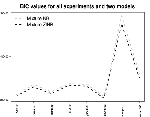
Figure 2: BIC values for mixture of two NB distributions (dashed grey line) and mixture of zero-inflated NB distribution for the background and NB distribution for the signal (dashed black line).

First of all, we have compared the fit of a NB mixture model, where a NB distribution is chosen both for the background and signal, against a ZINB-NB mixture, where a zero-inflated NB is considered for the background and a NB distribution for the signal. In Figure 2, we give the BIC values for the eight experiments, where we do not consider Markov properties. In general, we find that the BIC values are lower for the ZINB-NB mixture than for the NB mixture, suggesting a better fit for the zero-inflated mixture. In the following, we will therefore use zero-inflated distributions, differently to iSeq (Mo, 2012) and BayesPeak (Spyrou et al., 2009), which use Poisson and NB mixtures, respectively. FIGURE 2 ABOUT HERE.

Within the eight data sets that we analyzed, CBPT0, p300T0, WangCBP and Wangp300, are single experiments, i.e. with no replicates. We therefore compare the proposed MRF model with iSeq and BayesPeak on these four experiments. Table 4 gives the number of enriched regions identified by the three methods, respectively. For simplicity we provide the results only for chromosome 21. At the same 5% FDR, MRF can detect more regions than any of the other two methods. The overlap for all three methods is shown in the last row of the table, whereas pairwise comparisons are shown in the Venn diagrams in Figure 3 for two representative experiments (CBPT0 and p300T0). In general, MRF tends to agree more with iSeq than with BayesPeak in the sense that MRF identifies most of regions that also identified by iSeq. This is consistent with what we observed in the simulation study, where we also showed a lower false non-discovery rate for MRF. Furthermore, Figure 3 shows how the overlap between MRF and iSeq and the overlap between MRF and BayesPeak are both much bigger than the overlap between iSeq and BayesPeak. TABLE 4 and FIGURE 3 ABOUT HERE.

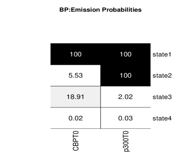
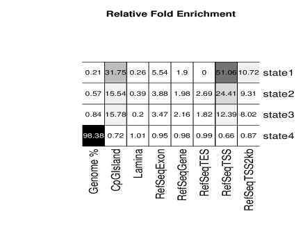
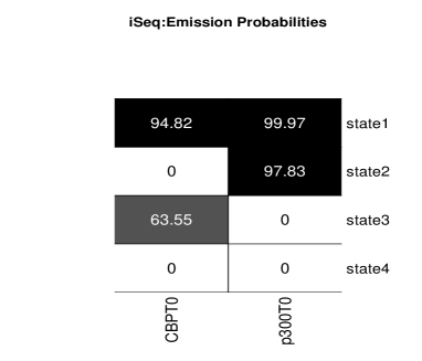
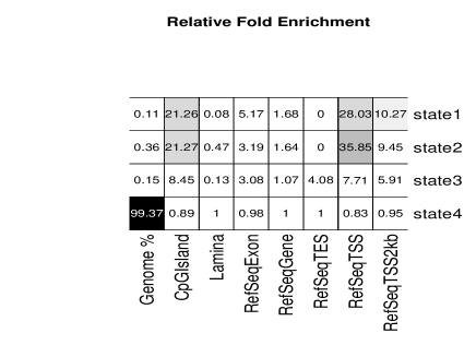
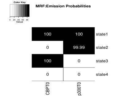
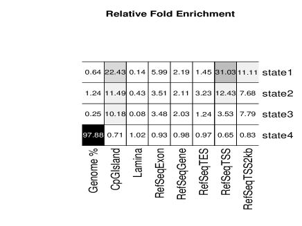
Figure 4: Validation of the enriched bins detected by BayesPeak (BP, top), iSeq (middle) and MRF (bottom) for CBPT0 and p300T0, using ChromHMM with a 4-state hidden Markov model. The left plots show heatmaps of the probabilities (in %) that the detected bins are enriched given each identified chromatin-state. The right plots show the relative percentage of the genome represented by each chromatin state (column 1) and the relative fold enrichment for several types of annotation (columns 2-8).

CBP and p300 both have largely overlapping roles in transcriptional activation. We use ChromHMM (Ernst and Kellis, 2010) to explore whether the regions identified by MRF are likely functional in transcription activation and whether different chromatin features are enriched in the regions identified by the different methods. Figure 4 shows the results of ChromHMM using a 4-state hidden Markov model on the enrichment profile given by the three methods, each at a 5% FDR, for two representative experiments (CBPT0 and p300T0). For each method, the data from the two proteins is jointly modelled by ChromHMM. The left plots give the emission probabilities for the different analyses, that is the probability of the observed enrichment given each of the four possible states. These plots show how, for all analyses, three of the four states explain most of the enrichment pattern in the identified lists. The right plots give the relative fold enrichment for several annotations. These plots show how these three states are represented by a similar enrichment of features for the three methods, mainly CpGisland and RefSeq Transcription Start Sites (RefSeqTSS), suggesting that the additional regions detected by MRF are likely to be genuine binding events. FIGURE 4 ABOUT HERE.

For replicated experiments (CBPT301, CBPT302, p300T301, p300T302), we compare the proposed MRF model for multiple experiments, with our previously developed mixture model (Bao et al., 2013). In both cases, we detect the enriched regions and the differentially bound regions, that is the regions bound only by one of the two proteins, at a 5% FDR. Table 5 reports the results for chromosome 21. The results show that by including the assumption of Markov properties, the number of enriched regions detected is larger than when the Markov property is not considered. This is to be expected since regions with a relatively small number of counts but with neighbouring enriched regions may not be detected by the mixture model but would be detected by the MRF model. Similarly to before, Figure 5 shows the results of ChromHMM using a 4-state hidden Markov model on the enrichment profile given by MRF and the mixture model, each at a 5% FDR. The emission probabilities (left) show how, for all analyses, two of the three states explain most of the enrichment pattern in the identified lists. The relative fold enrichment plots (right) show how these two states seem to be mostly enriched with TSS and CpGIsland features for both methods. Together with the results in Table 5, one can conclude that by taking into account Markov properties while combining replicates, many more regions are found at the same FDR, and that these regions are of the same nature as those found by the mixture model. TABLE 5 and FIGURE 5 ABOUT HERE.

It is expected that p300 and CBP should have roughly the same number of binding sites (Bao et al., 2013). In this case, one can impose this constraint in the model, as discussed in section 2.4. Table 6 reports the number of enriched and differentially bound regions for chromosome 21 under the assumption that the two proteins, CBP and p300, have the same number of binding sites under the same condition (here the time point). In Bao et al. (2013), we show how this approach helps to account for the different IP efficiencies of individual experiments, particularly in cases where there are no technical replicates and therefore it is more difficult to give an accurate estimate for the proportion of binding sites. TABLE 6 ABOUT HERE.

5 Conclusion

In this paper, we propose a one-dimensional Markov random field model for the analysis of ChIP-seq data. Our model can be viewed as a hidden Markov model where the initial distribution is the stationary distribution. As such, we follow the literature on existing HMM-based models, such as BayesPeak (Spyrou et al., 2009) and iSeq (Mo, 2012). Similarly to these models, we capture the spatial dependencies of local bins by an assumption of first-order Markov properties. Differently to these methods, we develop a joint model for multiple ChIP-seq experiments under general experimental designs, such as experiments with replicates and different antibodies. The resulting joint model is expected to lead to a more robust detection of enriched and differentially bound regions. Furthermore, similarly to our previously developed mixture model (Bao et al., 2013), we show how a priori knowledge of the same number of binding sites for different proteins can also be added to the model, in order to better account for the different ChIP efficiencies of individual experiments. Finally, we advocate the use of zero-inflated distributions for the background distribution, as these better account for the large number of zeros in the data.

In an extensive simulation study, we show how the proposed Markov random field model is in general superior to both iSeq and BayesPeak, as it achieves a lower false non-discovery rate at the same false discovery rate. When the data are generated from the same model used by iSeq, i.e. an Ising model with one parameter and a Poisson mixture, the methods perform similarly well, but RFM performs better than iSeq and BayesPeak under more general mixture distributions and model assumptions. Finally, we present an analysis on real data for the detection of histone modifications of two transcriptional activators from eight ChIP-sequencing experiments, including technical replicates with different IP efficiencies.

6 Software

The method is available in the R package enRich, which can be currently downloaded from http://people.brunel.ac.uk/~mastvvv/Rcode/enRich_2.0.tar.gz.

7 Supplementary Material

Supplementary material is available online at http://biostatistics.oxfordjournals.org.

Figure 1: Plots of bin counts $Y_{m}$ versus bin $m$ (left) for bins of size 200bp on a region of chromosome 1 for the p300T302 experiment, and $P(X_{m}=1|Y_{m},{\hat{\theta}})$ versus bin $m$ (right) under mixture of NB model.

Figure 3: Venn diagrams of the number of enriched regions detected by MRF, iSeq and BayesPeak (BP) at the 5% FDR, for the CBPT0 and p300T0 experiments.

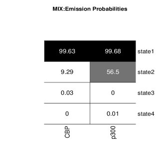
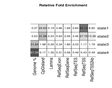
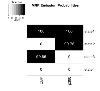
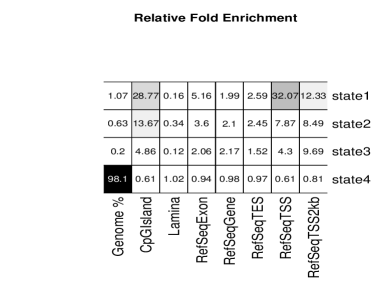
Figure 5: Validation of the enriched bins detected by mixture model (MIX, top) and MRF (bottom) for technical replicates of CBP and p300 at time T30, using a 4-state ChromHMM. The left plots show heatmaps of the probabilities (in %) that the detected bins are enriched given each identified chromatin-state. The right plots show the relative percentage of the genome represented by each chromatin state (column 1) and the relative fold enrichment for several types of annotation (columns 2-8).

Table 1: Conditional frequencies of enrichment given that the previous bin is enriched or not, denoted by $f_{1|1}$ and $f_{1|0}$ respectively. A region is called enriched or not using a latent mixture model at a 5% FDR.

Experiment	$f_{1|1}$	$f_{1|0}$
CBPT0	0.0909	0.0002
CBPT301	0.3004	0.0008
CBPT302	0.4924	0.0017
p300T0	0.3342	0.0021
p300T301	0.4015	0.0020
p300T302	0.5653	0.0027
Wang CBP	0.4129	0.0014
Wang p300	0.2190	0.0005

Table 2: Simulated count data is generated for $M=10000$ regions under four different scenarios. The table reports the average FNDR over 100 iterations, at a controlled FDR of 5%, for MRF, iSeq and BayesPeak. The p-values show whether the MRF model has a significantly lower FNDR.

	Less Efficient Experiment		More Efficient Experiment
	Scenario 1: ZINB-NB mixture with $\tilde{q}_{1}+\tilde{q}_{0}\neq 1$ (as MRF).
	Signal: NB(1.38,2.07)		Signal: NB(6.95,0.89)
	Background: ZINB(0.66, 0.33, 2.01)		Background: ZINB(0.53, 0.36, 0.88)
	$(\tilde{q}_{0},\tilde{q}_{1})$=(0.002,0.940)		$(\tilde{q}_{0},\tilde{q}_{1})$=(0.003,0.866)
	FNDR	p-value	FNDR	p-value
MRF	0.0090	-	0.0020	-
iSeq	0.0086	0.7778	0.0052	$<2.2e-16$
BayesPeak	0.0292	$<2.2e-16$	0.0088	$<2.2e-16$
	Scenario 2: Poisson-Poisson mixture with $\tilde{q}_{1}+\tilde{q}_{0}=1$ (as iSeq).
	Signal: Poisson(1.5)		Signal: Poisson(9.0)
	Background: Poisson(0.5)		Background: Poisson(0.5)
	$\tilde{q}_{1}=1-\tilde{q}_{0}=0.98$		$\tilde{q}_{1}=1-\tilde{q}_{0}=0.98$
	FNDR	p-value	FNDR	p-value
MRF	0.0606	-	3.79e-06	-
iSeq	0.0586	0.7661	1.04e-05	0.1073
BayesPeak	0.4547	$<2.2e-16$	0.2707	$<2.2e-16$
	Scenario 3: Poisson-Poisson mixture with $\tilde{q}_{1}+\tilde{q}_{0}\neq 1$.
	Signal: Poisson(3.0)		Signal: Poisson(6.0)
	Background: Poisson(0.5)		Background: Poisson(0.2)
	$(\tilde{q}_{0},\tilde{q}_{1})=(0.02,0.5)$		$(\tilde{q}_{0},\tilde{q}_{1})=(0.02,0.5)$
	FNDR	p-value	FNDR	p-value
MRF	0.0225	-	0.0011	-
iSeq	0.0287	$<2.2e-16$	0.0016	$1.737e-12$
BayesPeak	0.0299	$<2.2e-16$	0.0200	$<2.2e-16$
	Scenario 4: ZINB-NB mixture with $\tilde{q}_{1}+\tilde{q}_{0}=1$.
	Signal: NB(3.0, 1.0)		Signal: NB(6.0, 1.0)
	Background: ZINB(0.5, 0.5,0.5)		Background: ZINB(0.5, 0.5,0.5)
	$(\tilde{q}_{0},\tilde{q}_{1})=(0.02,0.98)$		$(\tilde{q}_{0},\tilde{q}_{1})=(0.02,0.98)$
	FNDR	p-value	FNDR	p-value
MRF	0.0168	-	0.0039	-
iSeq	0.2903	$<2.2e-16$	0.1874	$<2.2e-16$
BayesPeak	0.4100	$<2.2e-16$	0.4310	$<2.2e-16$

Table 3: Simulated count data are generated for $M=10000$ regions and for two replicates from a ZINB-NB under two different scenarios (with and without Markov property). The table reports the average FNDR over 100 iterations, at a controlled FDR of 5%, for MRF and a mixture model. The p-values show whether the MRF model has a significantly lower FNDR.

	Less Efficient Experiment		More Efficient Experiment
	Scenario 5: multiple experiments and Markov property.
	Rep 1 – Signal: NB(2.738, 1.548)		Rep 1 – Signal: NB(3.797, 1.139)
	Rep 2 – Signal: NB(5.991, 0.957)		Rep 2 – Signal: NB(7.392, 0.955)
	Rep 1 – BG: ZINB(0.634, 0.430, 2.322)		Rep 1 – BG: ZINB(0.656, 0.393, 3.014)
	Rep 2 – BG: ZINB(0.481, 0.477, 1.246)		Rep 2 – BG: ZINB(0.486, 0.395, 1.061)
	$(\tilde{q}_{0},\tilde{q}_{1})=(0.003,0.839)$		$(\tilde{q}_{0},\tilde{q}_{1})=(0.003,0.830)$
	FNDR	p-value	FNDR	p-value
MRF	0.0011	-	0.0008	-
Mixture	0.0072	$<2.2e-16$	0.0057	$<2.2e-16$
	Scenario 6: multiple experiments and no Markov property.
	Rep 1 – Signal: NB(2.738, 1.548)		Rep 1 – Signal: NB(3.797, 1.139)
	Rep 2 – Signal: NB(5.991, 0.957)		Rep 2 – Signal: NB(7.392, 0.955)
	Rep 1 – BG: ZINB(0.634, 0.430, 2.322)		Rep 1 – BG: ZINB(0.656, 0.393, 3.014)
	Rep 2 – BG: ZINB(0.481, 0.477, 1.246)		Rep 2 – BG: ZINB(0.486, 0.395, 1.061)
	$p(X=1)=0.017$		$p(X=1)=0.020$
	FNDR	p-value	FNDR	p-value
MRF	0.0073	-	0.0058	-
Mixture	0.0073	$0.5001$	0.0058	$0.6738$

Table 4: Number of enriched regions identified by MRF, iSeq and BayesPeak for four single experiments.

Method	CBPT0	p300T0	WangCBP	Wangp300
MRF	2073	4393	1443	639
iSeq	488	1115	1126	326
BayesPeak	1102	1834	603	576
overlap	263	799	396	190

Table 5: Number of enriched and differentially bound regions identified by MRF and ZINB-NB mixture model from technical replicates of CBP and p300 at time 30.

	Enriched regions		Differentially bound regions
Method	CBPT30	p300T30	only CBP	only p300
MRF	2977	3970	69	347
Mixture	981	1848	29	395
overlap	971	1823	4	78

Table 6: Number of enriched and differentially regions identified by MRF under the assumption that the two proteins, CBP and p300, have the same number of binding sites at the same time point.

	Enriched regions		Differentially bound regions
	CBP	p300	only CBP	only p300
CBPT0 vs p300T0	1606	3842	23	336
CBPT30 vs p300T30	3146	4123	62	365
WangCBP vs Wangp300	1426	643	376	23

References

- Bao et al. (2013) Bao, Y., V. Vinciotti, E. Wit, and P. ’t Hoen (2013). Accounting for immunoprecipitation efficiencies in the statistical analysis of ChIP-seq data. Under revision.
- Bardet et al. (2012) Bardet, A., Q. He, J. Zeitlinger, and A. Stark (2012). A computational pipeline for comparative ChIP-seq analyses. Nature Protocols 7(1), 45–61.
- Ernst and Kellis (2010) Ernst, J. and M. Kellis (2010). Discovery and characterization of chromatin states for systematic annotation of the human genome. Nature Biotechnology 28(8), 817–825.
- Hoffman et al. (2012) Hoffman, M., J. Ernst, S. Wilder, A. Kundaje, R. Harris, M. Libbrecht, B. Giardine, P. Ellenbogen, J. Bilmes, E. Birney, R. Hardison, I. Dunham, M. Kellis, and W. Noble (2012). Integrative annotation of chromatin elements from ENCODE data. NAR 41(2), 827–841.
- Kuan et al. (2011) Kuan, P., D. Chung, G. Pan, J. Thomson, R. Stewart, and S. Keles (2011). A statistical framework for the analysis of ChIP-Seq data. JASA 106(495), 891–903.
- Mo (2012) Mo, Q. (2012). A fully Bayesian hidden Ising model for ChIP-seq data analysis. Biostatistics 13(1), 113–128.
- Qin et al. (2010) Qin, Z., J. Yu, J. Shen, C. Maher, M. Hu, S. Kalyana-Sundaram, Y. J., and A. Chinnaiyan (2010). HPeak: an hmm-based algorithm for defining read-enriched regions in chip-seq data. BMC Bioinformatics 11(369).
- Ramos et al. (2010) Ramos, Y., M. Hestand, M. Verlaan, E. Krabbendam, Y. Ariyurek, H. van Dam, G. van Ommen, J. den Dunnen, A. Zantema, and P. ’t Hoen (2010). Genome-wide assessment of differential roles for p300 and CBP in transcription regulation. NAR 38(16), 5396–5408.
- Scott (2002) Scott, S. (2002). Bayesian methods for hidden Markov models: Recursive computing in the 21st century. JASA 97(457), 337–351.
- Shao et al. (2012) Shao, Z., Y. Zhang, G. Yuan, S. Orkin, and D. Waxman (2012). MAnorm: a robust model for quantitative comparision of ChIP-Seq data sets. Genome Biology 13(3), R16.
- Spyrou et al. (2009) Spyrou, C., R. Stark, A. Lynch, and S. Tavare (2009). BayesPeak: Bayesian analysis of ChIP-seq data. BMC Bioinformatics 10(1), 299.
- Tuteja et al. (2009) Tuteja, G., P. White, J. Schug, and K. Kaestner (2009). Extracting transcription factor targets from ChIP-Seq data. NAR 37(17), e113.
- Wang et al. (2009) Wang, Z., C. Zang, K. Cui, D. Schones, A. Barski, W. Peng, and K. Zhao (2009). Genome-wide mapping of HATs and HDACs reveals distinct functions in active and inactive genes. Cell 138, 1019–1031.
- Zeng et al. (2013) Zeng, X., R. Sanalkumar, E. Bresnick, H. Li, Q. Chang, and K. S. (2013). jMOSAiCS: Joint analysis of multiple ChIP-seq datasets.