Conditional Stability for Single Interior Measurement

Abstract

An inverse problem to identify unknown coefficients of a partial differential equation by a single interior measurement is considered. The equation considered in this paper is a strongly elliptic second order scalar equation which can have complex coefficients in a bounded domain with $C^{2}$ boundary and single interior measurement means that we know a given solution of the equation in this domain. The equation includes some model equations arising from acoustics, viscoelasticity and hydrology. We assume that the coefficients are piecewise analytic. Our major result is the local Hölder stability estimate for identifying the unknown coefficients. If the unknown coefficients is a complex coefficient in the principal part of the equation, we assumed a condition which we named admissibility assumption for the real part and imaginary part of the difference of the two complex coefficients. This admissibility assumption is automatically satisfied if the complex coefficients are real valued. For identifying either the real coefficient in the principal part or the coefficient of the 0-th order of the equation, the major result implies the global uniqueness for the identification.

1 Introduction

In order to make our description of the background more concise we first introduce two assumptions, and formulate the forward and inverse problems.

Assumption 1: Let $\Omega\subset\mathbb{R}^{n}$ $(2\leq n\in\mathbb{N})$ be a bounded domain with a $C^{2}$ smooth boundary $\partial\Omega$. Also, let $A(x)$ be a strictly positive Hermitian matrix on $\overline{\Omega}$ with entries in $C^{1}(\overline{\Omega})$ and $\gamma\in C^{1}(\overline{\Omega})$ be either a real valued positive or complex valued function with positive real and imaginary parts on $\overline{\Omega}$. Further, let $\rho\in C^{0}(\overline{\Omega})$ be a positive function on $\overline{\Omega}$ if $\gamma$ is a real valued function and complex valued function on $\overline{\Omega}$ with non-positive imaginary part if $\gamma$ is a complex valued function. In addition, if $\gamma$ and $\rho$ have any discontinuities in their derivatives, we assume that they are away from $\partial\Omega$. Let $g=g(x)\in H^{3/2}(\partial\Omega)$ and $\omega^{2}\geq 0$, where $H^{3/2}(\partial\Omega)$ is the Sobolev space of fractional differential order $3/2$ in the $L^{2}(\partial\Omega)$ sense.

Now for given Dirichlet data $g=g(x)$, we consider the following boundary value problem:

$$\left\{\begin{array}[]{ll}L_{\gamma}u:=\nabla\cdot\big{[}\gamma(x)A(x)\nabla u(x)\big{]}+\omega^{2}\rho(x)u(x)=0&\mbox{in }\Omega,\\ u(x)=g(x)&\mbox{on }\partial\Omega.\end{array}\right.$$ (1)

Assumption 2: When $\gamma$ and $\rho$ are real valued function, we assume that $\Omega$ is non-vibrating, that is (1) with $g=0$ only admits a trivial solution.

With the above given conditions in Assumptions 1 and 2 on $\Omega,\,\gamma,\,A,\,\rho,g$ and $\omega^{2}$, it is well known that there exists a unique solution $u=u(x)\in H^{2}(\Omega)$ to (1), where $H^{2}(\Omega)$ denotes the Sobolev space of differential order $2$ in the $L^{2}(\Omega)$ sense.

The Inverse Problem: We consider the following problem. Given the interior measurement $u(x)\,(x\in\Omega)$, the Dirichlet boundary condition $g\not\equiv 0$ on $\partial\Omega$, the coefficients $A,\,\rho$ on $\overline{\Omega}$, identify $\gamma$ in $\Omega$.

In this paper we will mainly consider the above inverse problem whose goal is to identify $\gamma$. However at the end of the paper we will address a somewhat easier alternate inverse problem where we assume all of the conditions above except that $\gamma$ is assumed known and our goal then will be to identify $\rho$. Natural questions, for both of our main inverse problem and the alternate inverse problem, are the uniqueness, stability and reconstruction of $\gamma$ (or $\rho$) from the measured data. Here our main result is a stability result for $\gamma$ given $\rho$ (or $\rho$ given $\gamma$).

There are two major backgrounds for this inverse problems. The one is coming from a newly developed imaging modality called MRE (magnetic resonance elastography) ([8]). It produces movies of shear waves induced by a single frequency excitation. Once a mathematical model of these waves is determined, analysis and mathematical algorithms can be developed, based on the mathematical model. The numerical implementation of the algorithms produces diagnostically useful images with the goal of adding to noninvasive medical diagnostic capabilities. In ([12]), e.g., the advance, through MRE, to produce early diagnosis of liver stiffness and fibrosis is described. MRE is in the general class of hybrid or coupled physics imaging technologies where two physical principles, here MRI and elastic wave propagation are combined to obtain a richer data set from which to obtain diagnostically rich images.

The above boundary value problem with $A$ equal to the identity matrix $I$ and $\operatorname{Im}\rho=0$ is the simplest PDE (partial differential equation) model which is used to describe a component $u$ of a shear wave inside human tissue. In (1), $\omega/(2\pi)$ is the angular frequency of the time harmonic vibration, $\mbox{Re}(e^{i\omega t}g(x))$, applied to a human body where $t$ is time. When $A$ is equal to the identity matrix $I$, and $\rho$ is real the functions $\rho$, $\mbox{Re}\,\gamma$ and $\mbox{Im}\,\gamma$ are the density, storage modulus and loss modulus of human tissue.

The other is coming from hydrology. This corresponds to the case $A=I$, and $\gamma$ is a real valued $C^{1}(\overline{\Omega})$ function and $\omega=0$, then this inverse problem has been studied in hydrology.

Next we discuss some known results. In the two dimensional case Alessandrini ([1]) gave a Hölder stability result for identifying $\gamma$ by analyzing the critical set, $\{x\in\Omega|\nabla u=0\}$ of, $u$, the solution to the forward problem (1). Further, if the zero on the right hand side of the partial differential equation in (1) is replaced by a positive, Hölder continuous function, $f$, on $\overline{\Omega}$, Richter ([10]) gave a Lipschitz stability result, in any dimension, for identifying $\gamma$ by showing the non-degeneracy of $\nabla u\neq 0$ and using the maximum principle. It should be noticed that the assumption, on the positivity of $f$, is a very strong assumption and is only a sufficient condition to guarantee the non-degeneracy of $\nabla u$. This assumption replaces the need to analyze the critical set. A number of other results have been established where the analysis of the critical set for a single data set is avoided by making additional hypotheses. Marching and elliptic algorithms for recovering an unknown real coefficient, $\gamma$, when $\rho$ is real and known in the interior, $A=I$, $u$ is given in the interior, and it is propagating there to one fixed direction which means that derivative of u in this direction does not vanish there are presented in ([13]).

Another method for addressing the problem of recovering $\gamma$, when data sets $u$ can have critical points, is the use of multiple measurements whose input can be controlled. If we can have multiple measurements and control the input, then the reconstruction of $\gamma$ was first given by Nakamura-Jiang-Nagayasu-Cheng ([9]) using complex geometric optic solutions and linking them to the input data by solving a Cauchy problem. In that paper, the regularity assumptions on $\gamma$, $\rho$ are just $\gamma\in C^{2}(\overline{\Omega})$, $\rho\in L^{\infty}(\Omega)$. When it can be assumed that multiple measurements are given, a more systematic analysis, for a wide class of hybrid inverse problems, was recently done by Bal-Uhlmann ([2], [3]). In this work the given mathematical model is linearized and then: (1) a reconstruction scheme for identifying all the coefficients $\gamma,A$ and $\rho$ of the linearized operator $L_{\gamma}$ is presented; and (2) a Lipschitz stability result is given when the regularity assumptions on $\gamma,\,A$ and $\rho$ are just Hölder continuous on $\overline{\Omega}$.

In the paper presented here, we are concerned with extending Alessandrini’s result to the higher dimensional case when $\gamma$ is a complex valued function and $\omega^{2}>0$. Even in the two dimensional case and if $\gamma$ is a real valued function, the cases $\omega=0$ and $\omega^{2}>0$ are quite different. One can see that Alessandrini’s argument breaks down for the case $\omega^{2}>0$. As far as we know, there is not any stability result known for the case where $\gamma$ is complex valued, where $\gamma$ can have discontinuous second derivatives and only one measurement, $u$, as opposed to multiple measurements, is given. We will show local Hölder stability of our inverse problem identifying $\gamma$ for the case $\gamma$ is a complex valued $C^{1}$ function on $\overline{\Omega}$ and piecewise analytic in $\Omega$ by assuming that $\rho$ is continuous on $\overline{\Omega}$ and piecewise analytic in $\Omega$ and $A$ is positive Hermitian and analytic.

This third assumption is given more precisely as follows. We denote by $\mathcal{A}^{(k)}(\Omega)$ (resp. $\mathcal{PA}^{(k)}(\Omega)$) the set of complex valued $C^{k}$ functions on $\overline{\Omega}$ which are analytic (resp. piecewise analytic) in $\Omega$ and now clarify our definition of piecewise analytic and further assumptions on $A,\,\rho,\,\gamma$.

Definition 1.1.

(Piecewise Analytic) A function $f$ is piecewise analytic in $\Omega$ if there exists a compact subset $S$ in $\Omega$ consisting of a finite disjoint union of closed smooth analytic hypersurfaces such that $f$ is analytic in $\Omega\setminus S$ and is locally extendable as an analytic function from one side of $S$ across to the other side. That is, for any $x\in S$, we can find an open neighborhood $V$ of $x$ with $V\setminus S$ consisting of two connected components $V_{1}$ and $V_{2}$ for which $f$ in $V_{1}$ (resp. $V_{2}$) analytically extends to $V$.

Assumption 3: Let $A\in M(n;\,\mathcal{A}^{(1)}(\Omega))$, $\gamma\in\mathcal{PA}^{(1)}(\Omega)$, $\rho\in\mathcal{PA}^{(0)}(\Omega)$ and the locations of the singularities of $\gamma$ and $\rho$ be the same. Here $A\in M(n;\,\mathcal{A}^{(1)}(\Omega))$ means that all the entries of $n\times n$ matrix $A$ belong to $\mathcal{A}^{(1)}(\Omega)$.

With Assumptions 1,2, and 3 it can be shown by using the theories of analytic pseudo-differential operators, the theories for coercive boundary value problems and the fact that when $\gamma$ and $\rho$ are real we assume that we have a nonvibrating problem, that the unique solution $u\in H^{1}(\Omega)$ to (1) belongs to $\mathcal{PA}^{(1)}(\Omega)$. This follows because the interior transmission problem can be transformed to a coercive boundary value problem for a system of equations by introducing the boundary normal coordinates in the neighborhood $V$ of $x\in S$ (see Definition above) so that we can reflect the component $V_{1}\subset V$ to the other side of $S$ where we have the component $V_{2}\subset V$, and then apply the analytic hypo-ellipticity result given in Chapters III and V of [11] to this coercive boundary value problem.

Now let $\sigma>0$ be a sufficiently small constant. Furthermore, we introduce the notion of an admissible pair for functions on $\overline{\Omega}$.

Definition 1.2.

(Admissible Pair) A pair $(\gamma_{1},\,\gamma_{2})$ of functions on $\overline{\Omega}$ is said to be admissible if there exist exceptional angles $\kappa_{1}<\kappa_{2}<\dots<\kappa_{\ell}<\kappa_{\ell+1}=\kappa_{1}+2\pi$ with $\kappa_{k+1}-\kappa_{k}\leq\pi-\sigma$ $(k=1,\dots,\ell)$ such that, for any $k=1,\dots,\ell$,

$${}H_{n-1}\left(\left\{x\in\overline{\Omega}\,:\,(\gamma_{2}-\gamma_{1})(x)\neq 0,\,\,\operatorname{arg}\,(\gamma_{2}-\gamma_{1})(x)\equiv\kappa_{k}\mod 2\pi\right\}\right)=0.$$ (2)

Here $H_{n-1}$ denotes the $(n-1)$-dimensional Hausdorff measure.

Clearly the fact that $\ell\geq 3$ follows from definition. In addition, we make the following remarks.

Remark:
(i) Here we give a sufficient condition in order that $\gamma_{j},\,j\,=\,1,2$ is an admissible pair: Suppose there exists a non-negative constant $\kappa<(\pi-\sigma)/2$ satisfying

$$|\operatorname{Im}\,(\gamma_{2}-\gamma_{1})(x)|\leq\tan(\kappa)\,|\operatorname{Re}\,(\gamma_{2}-\gamma_{1})(x)|\qquad(x\in\overline{\Omega}),$$ (3)

then the pair $(\gamma_{1},\,\gamma_{2})$ becomes admissible. Note also, as a particular case, real valued $(\gamma_{1},\,\gamma_{2})$ are always admissible. Furthermore $\gamma_{1},\gamma_{2}$ are always admissible if $\operatorname{Im}(\gamma_{2}-\gamma_{1})\equiv 0$.
(ii) In addition to the lower bound on $\ell$, given in the definition of Admissible Pair, we can also assume without loosing its generality that $\ell\leq 4$. To see this suppose that $\kappa_{1},\dots,\kappa_{\ell}$ are the exceptional angles of the admissible pair $(\gamma_{1},\,\gamma_{2})$ for which (2) holds. We will show that if $\ell\geq 5$, there exists a $k$ with $\kappa_{k+2}-\kappa_{k}\leq\pi-\sigma$ so that $\kappa_{k+1}$ can be eliminated. Suppose that no such $k$ exists for some $\ell\geq 5$. Then $\kappa_{k+2}-\kappa_{k}>\pi-\sigma$ holds for every $k$ where we set $\kappa_{k+\ell}:=\kappa_{k}+2\pi$ for convenience. Clearly we have

$$2(\kappa_{\ell+1}-\kappa_{1})=\sum_{k=1}^{\ell}(\kappa_{k+2}-\kappa_{k})>\ell(\pi-\sigma)\geq 5(\pi-\sigma),$$

which contradicts the fact $\kappa_{\ell+1}-\kappa_{1}=2\pi$.

In order to state our main result, it is convenient to use the Sobolev space ${W^{q,p}(\Omega)}$ of differential order $q$ in the $L^{p}(\Omega)$ sense with the norm $||\cdot||_{W^{q,p}(\Omega)}$. We also set $||B||_{W^{q,p}(\Omega)}:=\sum_{i,j}||b_{i,j}||_{W^{q,p}(\Omega)}$ for a matrix $B(x)=(b_{i,j}(x))$. We denote by $u_{k}\in H^{2}(\Omega)\,(k=1,2)$ the solutions to the boundary value problem (1) with $\gamma=\gamma_{k},\,g=g_{k}\not\equiv 0\,(k=1,2)$ and $L_{k}=L_{\gamma_{k}}\,(k=1,2)$.

Then, we have our main result.

Theorem 1.3.

(Main Theorem) Let $d>0$ and $\Omega_{d}:=\{x\in\Omega\,:\,\operatorname{dist}(x,\,\mathbb{R}^{n}\setminus\Omega)>d\}$. Let $\gamma_{1},\gamma_{2}$ be an admissible pair and $A,\rho,\gamma_{1},\gamma_{2},\omega^{2}$ satisfy Assumptions 1,2,3, with $||A||_{W^{1,\infty}(\Omega)}\leq\sigma^{-1}$ and $||\gamma_{k}||_{W^{1,\infty}(\Omega)}\leq\sigma^{-1},\,k=1,2$. Then there exist constants $C>0$ and $\alpha\in(0,1)$ depending only on $\Omega$, $d$, $\sigma$, $g_{1}$ and the coefficients of $L_{1}$ such that

$$\|\gamma_{2}-\gamma_{1}\|_{L^{\infty}(\Omega_{d})}\leq C\left(\|\gamma_{2}-\gamma_{1}\|_{L^{\infty}(\partial\Omega)}+\|u_{2}-u_{1}\|_{W^{2,1}(\Omega)}\right)^{\alpha}$$ (4)

for any $g_{2}$ and $\gamma_{2}$ of an admissible pair $(\gamma_{1},\,\gamma_{2})$. Furthermore, if $\Omega$ has an analytic smooth boundary and if $g_{1}$ is analytic in $\partial\Omega$ and all the coefficients of $L_{1}$ are analytic near $\partial\Omega$, then we have the estimate (4) in which $L^{\infty}(\Omega_{d})$ is replaced with $L^{\infty}(\Omega)$.

The succeeding sections are devoted to the proof of the main result and they are organized as follows. We first present a key identity and an associated estimate. Then, we give: (1) statements about a tubular neighborhood of the critical set of the solution, $u_{1}$, to (1), when $\gamma$ is replaced by $\gamma_{1}$; (2) the estimate of the $n$-dimensional Lebesgue measure of the tubular neighborhood; and (3) a lower estimate of $|\nabla u|$ outside this tubular neighborhood. The proofs of these results are given in Appendix. Combining the three sets of estimates we finish proving the main result. Finally we give the stability estimate for the alternate inverse problem which is to identify $\rho$ given $\gamma,A,\omega^{2}$, and $u$.

2 Key identity and an associated estimate

Let $\psi=\gamma_{2}-\gamma_{1}$ and $\nabla_{B}$ denote $B(x)\nabla$ for a matrix $B(x)$. Then, it is straightforward to establish the following key identity.

Lemma 2.1.

(Key Identity) Let Assumptions 1 and 2 be satisfied with $\gamma$ replaced by $\gamma_{k}$ and $g$ replaced by $g_{k},\,k=1,2$. Then, for any $\zeta\in H_{0}^{1}(\Omega)$, that is $\zeta\in H^{1}(\Omega)$ with trace $\zeta\Big{|}_{\partial\Omega}=0$, we have

$$\int_{\Omega}\psi\nabla{}_{A}\,u_{1}\cdot\nabla\zeta=-\int_{\Omega}\gamma_{2}\nabla{}_{A}\,(u_{2}-u_{1})\cdot\nabla\zeta+\omega^{2}\int_{\Omega}\rho(u_{2}-u_{1})\zeta.$$ (5)

Here $x\cdot y$ denotes a sum $\sum_{k=1}^{n}x_{k}y_{k}$ for $x,y\in\mathbb{C}^{n}$.

Based on this key identity, we have the following fundamental estimate associated to the key identity.

Proposition 2.2.

Let Assumptions 1,2, and 3 be satisfied with $\gamma$ replaced by $\gamma_{k}$ and $g$ replaced by $g_{k},\,k=1,2$. Then, there exists a constant $C>0$ depending only on $\Omega$, $\sigma$, $g_{1}$ and the coefficients of $L_{1}$ such that

$$\int_{\Omega}|\psi|\,\nabla{}_{A}\,u_{1}\cdot\overline{\nabla u_{1}}\leq C\left(\|\psi\|_{L^{\infty}(\partial\Omega)}+\|u_{2}-u_{1}\|_{W^{2,1}(\Omega)}\right).$$ (6)

Note that, as $A$ is a positive Hermitian matrix, the term $\nabla{}_{A}\,u_{1}\cdot\overline{\nabla u_{1}}$ takes non-negative real values.

Before we present the proof, taking advantage of our Assumptions 1 and 3, we first present several new sets and functions that we need for the estimate. Consider the map $\iota:\partial\Omega\times\mathbb{R}\to\mathbb{R}^{n}$ of $C^{1}$ class defined by $(y,s)\to y+s\nu(y)$ where $\nu(y)$ is a unit conormal vector of $\partial\Omega$ at $y$ pointing to $\Omega$. Then, as $\partial\Omega$ is compact, there exists an $\epsilon>0$ such that $\iota$ becomes a $C^{1}$ isomorphism between $\partial\Omega\times(-\epsilon,\epsilon)$ and an open neighborhood of $\partial\Omega$. Hence we have a family $\{U_{j}\}_{j\in\mathbb{N}}$ of relatively compact open subsets in $\Omega$ satisfying the conditions below:

1. $\Omega=\cup_{j}U_{j}$ and $U_{j}\subset\subset U_{j+1}\subset\subset\Omega$.

2. $U_{j}$ has a $C^{1}$ smooth boundary.

3. $H_{n-1}(\partial U_{j})\to H_{n-1}(\partial\Omega)$ ($j\to\infty$). We also have $\operatorname{dist}(\partial\Omega,\,\partial U_{j})\to 0$ when $j\to\infty$.

Furthermore, using the definition of subanalytic sets given in Appendix (see also ([4]), we can find a family $\{W_{j}\}_{j\in\mathbb{N}}$ of relatively compact subanalytic open subsets in $\Omega$ with $U_{j}\subset\subset W_{j}\subset\subset\Omega$. One choice for $W_{j}$ can be obtained by dividing $\mathbb{R}^{n}$ into sufficiently small n-dimensional cubes. Then $W_{j}$ can be selected to be a finite union of these cubes where each cube intersects $\overline{U_{j}}$ and where the closure of the finite union is contained in $\Omega$.

Now divide the complex plane, $\mathbb{C}$, into proper sectors

$$\Gamma_{k}:=\{z\in\mathbb{C}\setminus\{0\}\,:\,\kappa_{k}\leq\mbox{arg}\,z\leq\kappa_{k+1}\}\cup\{0\}\qquad(k=1,\dots,\ell).$$ (7)

Set

$$\widehat{\Omega}_{k}:=\{x\in\overline{\Omega}\,:\,\psi(x)\in\Gamma_{k}\},$$ (8)

and let $\theta_{k}(x)$ be the Lipschitz continuous function

$$\theta_{k}(x):=\left\{\begin{array}[]{ll}\operatorname{Re}\,\psi_{k}(x)-c_{k}\operatorname{Im}\,\psi_{k}(x)&\text{if }\operatorname{Im}\,\psi_{k}(x)\geq 0,\\ \\ \operatorname{Re}\,\psi_{k}(x)+c_{k}\operatorname{Im}\,\psi_{k}(x)&\text{if }\operatorname{Im}\,\psi_{k}(x)\leq 0,\end{array}\right.$$ (9)

where $\psi_{k}(x):=\exp(-(\kappa_{k}+\kappa_{k+1})i/2)\psi(x)$ and $c_{k}:=1/\tan((\kappa_{k+1}-\kappa_{k})/2)$. In addition, using the definition of subanalytic functions in Appendix, see also ([4]), $\theta_{k}$ is a subanalytic function on $\overline{W_{j}}$.

Furthermore it follows from the definition of $\theta_{k}(x)$ that we have

1. $\theta_{k}(x)<0$ if and only if $\psi(x)\in\mathbb{C}\setminus\Gamma_{k}$,

2. $\theta_{k}(x)=0$ if and only if $\psi(x)\in\partial\Gamma_{k}$,

3. $\theta_{k}(x)>0$ if and only if $\psi(x)\in\Gamma_{k}^{\circ}$.

Hence, in particular, a point $x$ belongs to $\widehat{\Omega}_{k}$ if and only if $\theta_{k}(x)\geq 0$ holds. We also define, for $h>0$,

$$\theta_{k,h}(x):=h^{-1}([\theta_{k}(x)]^{+}\wedge h),$$ (10)

where $[m]^{+}=\mbox{max}(m,\,0)$, $m\wedge\ell=\mbox{min}(m,\,\ell)$ for $m,\,\ell\in\mathbb{R}$. Then $\theta_{k,h}(x)$ is again a Lipschitz continuous subanalytic function on each $\overline{W}_{j}$ and it satisfies

$$0\leq\theta_{k,h}(x)\leq 1,\,\,\,\operatorname{supp}\theta_{k,h}(x)\subset\widehat{\Omega}_{k},\,\,\,\lim_{h\to 0^{+}}\theta_{k,h}(x)\to\chi_{\{x\in\widehat{\Omega}_{k}\,:\,\theta_{k}(x)\neq 0\}}.$$ (11)

Here $\chi_{A}$ designates the characteristic function of a subset $A$.

Finally, let $\tau_{j,h}$ be a $C^{\infty}$ function in $\Omega$ satisfying $0\leq\tau_{j,h}(x)\leq 1$, $\tau_{j,h}(x)=0$ at $x\in\Omega$ with $\operatorname{dist}(x,\,\mathbb{R}^{n}\setminus U_{j})\leq 2^{-1}h$, $\tau_{j,h}(x)=1$ at $x\in\Omega$ with $\operatorname{dist}(x,\,\mathbb{R}^{n}\setminus U_{j})\geq h$ and $|\nabla\tau_{j,h}(x)|\leq C_{\tau}h^{-1}$ for some $C_{\tau}>0$. Note that, by choosing a suitable $\tau_{j,h}$ for each $j$, we may assume that the constant $C_{\tau}$ is independent of $j$.

Now we are ready to prove Proposition 2.2. In the proof we will make extensive use of the results in Appendix.

Proof.

Set

$$\zeta_{j,k,h}:=\overline{u}_{1}\tau_{j,h}\theta_{k,h}\qquad(k=1,\dots,\ell,\,j\in\mathbb{N}).$$ (12)

As $\zeta_{j,k,h}$ belongs to $H_{0}^{1}(\Omega)$ and $\operatorname{supp}\zeta_{j,k,h}\subset U_{j}$, by taking $\zeta_{j,k,h}$ as $\zeta$ in the key identity, and replacing $\Omega$ by $U_{j}$, we obtain

$$\left|\,\int_{U_{j}}\psi\tau_{j,h}\theta_{k,h}\nabla{}_{A}\,u_{1}\cdot\overline{\nabla u_{1}}\right| \leq\left|\,\int_{U_{j}}\psi\overline{u}_{1}\tau_{j,h}\nabla{}_{A}\,u_{1}\cdot\nabla\theta_{k,h}\right|+\left|\,\int_{U_{j}}\psi\overline{u}_{1}\theta_{k,h}\nabla{}_{A}\,u_{1}\cdot\nabla\tau_{j,h}\right|$$ (13)

$$\quad+\left|\,\int_{U_{j}}\gamma_{2}\nabla{}_{A}\,(u_{2}-u_{1})\cdot\nabla\zeta_{j,k,h}\right|+\omega^{2}\left|\,\int_{U_{j}}\rho(u_{2}-u_{1})\zeta_{j,k,h}\right|.$$

We will compute, when $h\to 0^{+}$, the limit of each of the five terms in (13), or the limit of estimates of each of the five terms.

Case 1: The limit of the term on the left hand side of (13).

It follows from (11) that we have

$$\lim_{h\rightarrow 0^{+}}\int_{U_{j}}\psi\tau_{j,h}\theta_{k,h}\nabla{}_{A}\,u_{1}\cdot\overline{\nabla u_{1}}=\int_{\{x\in\widehat{\Omega}_{k}\cap U_{j}\,:\,\theta_{k}(x)\neq 0\}}\psi\nabla{}_{A}\,u_{1}\cdot\overline{\nabla u_{1}}$$

Set $T:=\left\{x\in\overline{W}_{j}\,:\,\theta_{k}(x)=0,\,\psi(x)\neq 0\right\}$ which is a relatively compact subanalytic subset in $\mathbb{R}^{n}$. Then, by the admissible condition for the pair $(\gamma_{1},\,\gamma_{2})$, we have $\dim_{\mathbb{R}}T<n-1.$ Hence the $n$-dimensional volume of $T$ is zero (see Proposition 6.7 in Appendix) and we can conclude

$$\lim_{h\rightarrow 0^{+}}\int_{U_{j}}\psi\tau_{j,h}\theta_{k,h}\nabla{}_{A}\,u_{1}\cdot\overline{\nabla u_{1}}=\int_{\{x\in\widehat{\Omega}_{k}\cap U_{j}\,:\,\theta_{k}(x)\neq 0\}}\psi\nabla{}_{A}\,u_{1}\cdot\overline{\nabla u_{1}}=\int_{\widehat{\Omega}_{k}\cap U_{j}}\psi\nabla{}_{A}\,u_{1}\cdot\overline{\nabla u_{1}}$$

Case 2: The limit of the first term in the right-hand side of (13).

We will establish that this term tends to zero when $h\to 0^{+}$. To obtain our result we first note that it follows from Proposition 6.7 in Appendix that there exists a constant $M_{\theta_{k}}$ such that, for any $t\in\mathbb{R}$ with finite exceptional ones, we get

$$H_{n-1}(\{x\in U_{j}\,:\,\theta_{k}(x)=t\})\leq H_{n-1}(\{x\in W_{j}\,:\,\theta_{k}(x)=t\})\leq M_{\theta_{k}}.$$

Set

$$U_{j,k,h}:=\{x\in U_{j}\,:\,0<\theta_{k}(x)<h\}.$$

Then, by noticing the fact that $\theta_{k,h}(x)$ is locally constant in $U_{j}\setminus\overline{U_{j,k,h}}$, we have

$$\left|\,\,\int_{U_{j}}\psi\overline{u}_{1}\tau_{j,h}\nabla{}_{A}\,u_{1}\cdot\nabla\theta_{k,h}\right| =\left|\,\,\int_{\overline{U_{j,k,h}}\cap U_{j}}\psi\overline{u}_{1}\tau_{j,h}\nabla{}_{A}\,u_{1}\cdot\nabla\theta_{k,h}\right|$$

$$=\left|\,\int_{U_{j,k,h}}\psi\overline{u}_{1}\tau_{j,h}\nabla{}_{A}\,u_{1}\cdot\nabla\theta_{k,h}\right|.$$

Here the last equality follows from the fact that $\partial U_{j,k,h}\cap U_{j}$ has n-dimensional measure zero. To see this let $W_{j,k,h}:=\{x\in W_{j}\,:\,0<\theta_{k}(x)<h\}$. Then as $W_{j,k,h}$ is a subanalytic subset, we have $\operatorname{dim}_{\mathbb{R}}\partial W_{j,k,h}<n$. Hence the $n$-dimensional volume of $\partial W_{j,k,h}$ is zero. This can be seen, for example, by again utilizing Proposition 6.7 in Appendix. Then the inclusion $\partial U_{j,k,h}\cap U_{j}\subset\partial W_{j,k,h}\cap U_{j}$ yields the result.

Set

$$Z^{0}:=\{x\in W_{j}\,:\,\theta_{k}(x)=0,\,\psi(x)=0\},\,\,Z^{\times}:=\overline{\{x\in W_{j}\,:\,\theta_{k}(x)=0,\,\psi(x)\neq 0\}}$$

and we also set, for $\epsilon>0$,

$$Z_{\epsilon}^{0}:=\{x\in W_{j}\,:\,\operatorname{dist}(x,Z^{0})\leq\epsilon\},\,\,Z_{\epsilon}^{\times}:=\{x\in W_{j}\,:\,\operatorname{dist}(x,Z^{\times})\leq\epsilon\}.$$

Note that, by the admissible pair condition, we have $\operatorname{dim}_{\mathbb{R}}(Z^{\times})<n-1$. In the estimate

$$\left|\,\int_{U_{j,k,h}}\psi\overline{u}_{1}\tau_{j,h}\nabla{}_{A}\,u_{1}\cdot\nabla\theta_{k,h}\right| \leq\left|\,\int_{U_{j,k,h}\cap Z^{0}_{\epsilon}}\psi\overline{u}_{1}\tau_{j,h}\nabla{}_{A}\,u_{1}\cdot\nabla\theta_{k,h}\right|$$

$$\qquad+\left|\,\int_{U_{j,k,h}\setminus Z^{0}_{\epsilon}}\psi\overline{u}_{1}\tau_{j,h}\nabla{}_{A}\,u_{1}\cdot\nabla\theta_{k,h}\right|,$$

by using the co-area formula, we obtain estimates

$$\left|\,\int_{U_{j,h,k}\cap Z^{0}_{\epsilon}}\psi\overline{u}_{1}\tau_{j,h}\nabla{}_{A}\,u_{1}\cdot\nabla\theta_{k,h}\right| \leq\left(\sup_{x\in Z^{0}_{\epsilon}}|\psi(x)|\right)||(\overline{u}_{1}|\nabla{}_{A}\,u_{1}|)||_{L^{\infty}(\Omega)}\dfrac{1}{h}\int_{U_{j,k,h}}|\nabla\theta_{k}|$$ (14)

$$\leq\left(\sup_{x\in Z^{0}_{\epsilon}}|\psi(x)|\right)||(\overline{u}_{1}|\nabla{}_{A}\,u_{1}|)||_{L^{\infty}(\Omega)}M_{\theta_{k}}$$

and

$$\left|\,\int_{U_{j,k,h}\setminus Z^{0}_{\epsilon}}\psi\overline{u}_{1}\tau_{j,h}\nabla{}_{A}\,u_{1}\cdot\nabla\theta_{k,h}\right|\leq 2\sigma^{-1}||(\overline{u}_{1}|\nabla{}_{A}\,u_{1}|)||_{L^{\infty}(\Omega)}\dfrac{1}{h}\int_{U_{j,k,h}\setminus Z^{0}_{\epsilon}}|\nabla\theta_{k}|$$ (15)

$$\quad\leq 2\sigma^{-1}||(\overline{u}_{1}|\nabla{}_{A}\,u_{1}|)||_{L^{\infty}(\Omega)}\left|\left|H_{n-1}\left(\left\{x\in U_{j}\setminus Z^{0}_{\epsilon}\,:\,\theta_{k}(x)=t\right\}\right)\right|\right|_{L^{\infty}(\{t\in\mathbb{R}\,:\,0<t<h\})}.$$

For any $\epsilon^{\prime}>0$, we have $U_{j,k,h}\setminus Z^{0}_{\epsilon}\subset Z^{\times}_{\epsilon^{\prime}}\setminus Z^{0}_{\epsilon}$ if $h>0$ is sufficiently small. Therefore, by the fact that $\operatorname{dim}_{\mathbb{R}}Z^{\times}<n-1$, it follows from the second claim of Proposition 6.7 in Appendix that the right-hand side of (15) tends to zero when $h\to 0^{+}$. Hence we have obtained

$$\overline{\underset{h\to 0^{+}}{\lim}}\left|\,\int_{U_{j}}\psi\overline{u}_{1}\tau_{j,h}\nabla{}_{A}\,u_{1}\cdot\nabla\theta_{k,h}\right|\leq\left(\sup_{x\in Z^{0}_{\epsilon}}|\psi(x)|\right)||(\overline{u}_{1}|\nabla{}_{A}\,u_{1}|)||_{L^{\infty}(\Omega)}M_{\theta_{k}}.$$

Clearly we have $\displaystyle\sup_{x\in Z^{0}_{\epsilon}}|\psi(x)|\to 0$ $(\epsilon\to 0^{+})$, from which

$$\lim_{h\to 0^{+}}\left|\,\int_{U_{j}}\psi\overline{u}_{1}\tau_{j,h}\nabla{}_{A}\,u_{1}\cdot\nabla\theta_{k,h}\right|=0\,\,\,\;\;\;\mbox{immediately follows}.$$

Case 3: The limit of the second term on the right hand side of (13).

Set

$$\overline{U}_{j,h}:=\{x\in\overline{U_{j}}\,:\,\operatorname{dist}(x,\,\mathbb{R}^{n}\setminus U_{j})\leq h\}.$$

We have

$$\left|\,\int_{U_{j}}\psi\overline{u}_{1}\theta_{k,h}\nabla{}_{A}\,u_{1}\cdot\nabla\tau_{j,h}\right| =\left|\,\,\int_{\overline{U}_{j,h}\cap U_{j}}\psi\overline{u}_{1}\theta_{k,h}\nabla{}_{A}\,u_{1}\cdot\nabla\tau_{j,h}\right|$$

$$\leq\left(\sup_{x\in\overline{U}_{j,h}}|\psi(x)|\right)||(\overline{u}_{1}|\nabla{}_{A}\,u_{1}|)||_{L^{\infty}(\Omega)}\dfrac{C_{\tau}}{h}\operatorname{vol}(\overline{U}_{j,h}).$$

As $\partial U_{j}$ is $C^{1}$ smooth, we get $\underset{h\to 0^{+}}{\lim}h^{-1}\operatorname{vol}(\overline{U}_{j,h})=H_{n-1}(\partial U_{j})$. Hence we have

$$\underset{h\to 0^{+}}{\overline{\lim}}\left|\,\int_{U_{j}}\psi\overline{u}_{1}\theta_{k,h}\nabla{}_{A}\,u_{1}\cdot\nabla\tau_{j,h}\right|\leq\left(C_{\tau}H_{n-1}(\partial U_{j})||(\overline{u}_{1}|\nabla{}_{A}\,u_{1}|)||_{L^{\infty}(\Omega)}\right)||\psi||_{L^{\infty}(\partial U_{j})}.$$

Case 4: The limit of the last two terms of (13).

Our Assumptions imply that $u_{2}-u_{1}$ is in $H^{2}(\Omega)=W^{2,2}(\Omega)$. Hence, we have

$$\quad\left|\,\,\int_{U_{j}}\gamma_{2}\nabla{}_{A}\,(u_{2}-u_{1})\cdot\nabla\zeta_{j,k,h}\right|+\omega^{2}\left|\,\,\int_{U_{j}}\rho(u_{2}-u_{1})\zeta_{j,k,h}\right|$$

$$\qquad\qquad=\left|\,\,\int_{U_{j}}\operatorname{div}(\gamma_{2}\nabla_{A}(u_{2}-u_{1}))\zeta_{j,k,h}\right|+\omega^{2}\left|\,\,\int_{U_{j}}\rho(u_{2}-u_{1})\zeta_{j,k,h}\right|$$

$$\qquad\qquad\leq\left(2\sigma^{-2}+\omega^{2}||\rho||_{L^{\infty}(\Omega)}\right)||u_{2}-u_{1}||_{{W^{2,1}}(\Omega)}.$$

The last step: Combining Cases 1-4.

Summing up, we have, for $k=1,\dots,\ell$,

$$\left|\,\,\int_{\widehat{\Omega}_{k}\cap U_{j}}\psi\nabla{}_{A}\,u_{1}\cdot\overline{\nabla u_{1}}\,\,\right|\leq C_{j}\left(||\psi||_{L^{\infty}(\partial U_{j})}+||u_{2}-u_{1}||_{W^{2,1}(\Omega)}\right),$$ (16)

where $C_{j}:=\max\left\{C_{\tau}H_{n-1}(\partial U_{j})||(\overline{u}_{1}|\nabla{}_{A}\,u_{1}|)||_{L^{\infty}(\Omega)},\,\,2\sigma^{-2}+\omega^{2}||\rho||_{L^{\infty}(\Omega)}\right\}.$ Now, by letting $j\to\infty$, we obtain

$$\left|\,\,\int_{\widehat{\Omega}_{k}}\psi\nabla{}_{A}\,u_{1}\cdot\overline{\nabla u_{1}}\,\,\right|\leq C\left(||\psi||_{L^{\infty}(\partial\Omega)}+||u_{2}-u_{1}||_{W^{2,1}(\Omega)}\right)$$ (17)

with

$$C:=\max\left\{C_{\tau}H_{n-1}(\partial\Omega)||(\overline{u}_{1}|\nabla{}_{A}\,u_{1}|)||_{L^{\infty}(\Omega)},\,\,2\sigma^{-2}+\omega^{2}||\rho||_{L^{\infty}(\Omega)}\right\}.$$ (18)

Then, by noticing the fact

$$|\psi(x)|\leq\dfrac{1}{\sin(\sigma/2)}\operatorname{Re}\,\beta_{k}\psi(x)\quad(x\in\widehat{\Omega}_{k})$$ (19)

with $\beta_{k}:=\exp(-(\kappa_{k+1}+\kappa_{k})i/2)$ because of $\psi(x)\in\Gamma_{k}$ for any $x\in\widehat{\Omega}_{k}$, we obtain

$$\int_{\Omega}|\psi|\nabla{}_{A}\,u_{1}\cdot\overline{\nabla u_{1}}\leq\sum_{k=1}^{\ell}\int_{\widehat{\Omega}_{k}}|\psi|\nabla{}_{A}\,u_{1}\cdot\overline{\nabla u_{1}}\leq\dfrac{1}{\sin(\sigma/2)}\sum_{k=1}^{\ell}\operatorname{Re}\int_{\widehat{\Omega}_{k}}\beta_{k}\psi\nabla{}_{A}\,u_{1}\cdot\overline{\nabla u_{1}}$$

$$\quad=\dfrac{1}{\sin(\sigma/2)}\sum_{k=1}^{\ell}\left|\operatorname{Re}\int_{\widehat{\Omega}_{k}}\beta_{k}\psi\nabla{}_{A}\,u_{1}\cdot\overline{\nabla u_{1}}\right|\leq\dfrac{1}{\sin(\sigma/2)}\sum_{k=1}^{\ell}\left|\,\int_{\widehat{\Omega}_{k}}\beta_{k}\psi\nabla{}_{A}\,u_{1}\cdot\overline{\nabla u_{1}}\right|$$

$$\quad=\dfrac{1}{\sin(\sigma/2)}\sum_{k=1}^{\ell}\left|\,\int_{\widehat{\Omega}_{k}}\psi\nabla{}_{A}\,u_{1}\cdot\overline{\nabla u_{1}}\right|\leq\dfrac{4C}{\sin(\sigma/2)}\left(||\psi||_{L^{\infty}(\partial\Omega)}+||u_{2}-u_{1}||_{W^{2,1}(\Omega)}\right).$$

This completes the proof. ∎

3 The Critical set of $u_{1}$

We consider first the case where $\Omega$ has $C^{2}$ boundary $\partial\Omega$. In this case let $V$ and $W$ be relatively compact open subsets in $\Omega$ satisfying

1. $\Omega_{d}\subset V\subset W\subset\subset\Omega$.

2. $V$ has a $C^{1}$ smooth boundary.

3. $W$ is a subanalytic subset in $\mathbb{R}^{n}$.

These $V$ and $W$ can be constructed by using the argument following the statements before the proof of Proposition 2.2.

Lemma 3.1.

(The Tubular Neighborhood of the Critical Set) Let $Z$ be the critical set of $u_{1}$ in $\overline{W}$. That is

$$Z=\{x\in\overline{W}\,:\,\nabla u_{1}(x)=0\}.$$ (20)

Then, there exist a family $U(\eta)\,(0<\eta\leq 1)$ of subanalytic open neighborhoods of $Z$, positive constants $r$ and $C_{j}\,(1\leq j\leq 3)$, where $C_{j}$ is independent of $\eta$ such that

• $\operatorname{vol}(U(\eta))\leq C_{1}\eta\quad\,\,(\eta\in(0,1]).$

• $\operatorname{dist}(x,\,Z)\geq C_{2}\eta\quad\,\,(x\in\mathbb{R}^{n}\setminus U(\eta),\,\eta\in(0,1]).$

• $\nabla{}_{A}\,u_{1}\cdot\overline{\nabla u_{1}}\geq C_{3}\operatorname{dist}(x,\,Z)^{r}\quad\,\,(x\in\overline{V}).$

Proof.

We first note that, as $u_{1}$ is piecewise analytic in an open neighborhood of $\overline{W}$, the function $\nabla{}_{A}\,u_{1}\cdot\overline{\nabla u_{1}}$ is subanalytic on $\overline{W}$ and $Z$ is a compact subanalytic subset in $\mathbb{R}^{n}$. Furthermore, since $g_{1}$ is non-zero, by the unique continuation property of a solution for $L_{1}$, we have $\operatorname{dim}_{\mathbb{R}}Z<n$. Hence, by the two Theorems in Appendix, for every $\eta,\;0<\eta\leq 1$, there exists $U(\eta)$, a subanalytic open neighborhood of $Z$ and positive constants $r$ and $C_{j}\,(1\leq j\leq 3)$ such that

• $\mbox{vol}(U(\eta))\leq C_{1}\eta\quad\,\,(\eta\in(0,1]).$

• $\mbox{dist}(x,\,Z)\geq C_{2}\eta\quad\,\,(x\in\mathbb{R}^{n}\setminus U(\eta),\,\eta\in(0,1]).$

• $\nabla{}_{A}\,u_{1}\cdot\overline{\nabla u_{1}}\geq C_{3}\mbox{dist}(x,\,Z)^{r}\quad\,\,(x\in\overline{V})$.

Hence the proof is complete. ∎

When $\partial\Omega$ is analytic smooth, $g_{1}$ is analytic in $\partial\Omega$ and all the coefficiens of $L_{1}$ are analytic near $\partial\Omega$, $\nabla{}_{A}\,u_{1}\cdot\overline{\nabla u_{1}}$ is a subanalytic function on $\overline{\Omega}$ and the subset $Z=\{x\in\overline{W}\,:\,\nabla u_{1}(x)=0\}$ is compact and subanalytic in ${\mathbb{R}}^{n}$. In this case then the conclusions of the lemma hold in all of $\overline{\Omega}$.

4 The final steps in the proof of the Main Theorem

We will use the estimate in Proposition 2.2 and the properties of the critical set of $u_{1}$, given above, to estimate $\int_{\Omega_{d}}|\psi|$ when $\partial\Omega$ is a $C^{2}$ boundary of $\Omega$ and to estimate $\int_{\Omega}|\psi|$ when $\partial\Omega$ is of $C^{2}$. We begin with the case where $\partial\Omega\in C^{2}$ and let $V$ be as defined in the previous section. In this case, for any $\eta\in(0,1]$, we have

$$\begin{array}[]{ll}\int_{V}|\psi|&\leq\int_{V\cap U(\eta)}|\psi|+\int_{V\setminus U(\eta)}|\psi|\\ \\ &\leq C_{1}\eta\|\psi\|_{L^{\infty}(V)}+(C_{2}^{r}C_{3})^{-1}\eta^{-r}\int_{V}|\psi|\,\nabla{}_{A}\,u_{1}\cdot\overline{\nabla u_{1}}.\end{array}$$ (21)

Then, minimizing (21) with respect to $\eta\in(0,1]$ and possibly making $C_{1}$ larger in order to ensure that $\eta\;\in\;(0,1]$ we have

$$\int_{V}|\psi|\leq C\|\psi\|_{L^{\infty}(V)}^{r/(r+1)}\left(\int_{V}|\psi|\,\nabla{}_{A}\,u_{1}\cdot\overline{\nabla u_{1}}\right)^{1/(r+1)}$$ (22)

for some constant $C>0$ depending only on $g_{1}$, $V$, and the coefficients of $L_{1}$.

As $V$ satisfies the cone condition, by the Gagliardo-Nirenberg inequality, there exists a constant $C^{\prime}{}>0$ depending only on $V$ such that for any $s>n$, we have

$$\|\psi\|_{L^{\infty}(V)}\leq C^{\prime}{}\|\psi\|_{W^{1,s}(V)}^{\theta}\|\psi\|_{L^{1}(V)}^{1-\theta}\leq{C_{\psi}}^{\prime}{}\|\psi\|_{L^{1}(V)}^{\kappa},$$ (23)

where $\theta=n/(n+1-n/s)$, ${C_{\psi}}^{\prime}{}=C^{\prime}{}\|\psi\|_{W^{1,s}(V)}^{\theta}$ and $\kappa=1-\theta$. Combining (22) and (23), we have

$$\|\psi\|_{L^{\infty}(\Omega_{d})}\leq\|\psi\|_{L^{\infty}(V)} \leq C_{\psi}\left(\int_{V}|\psi|\,\nabla{}_{A}\,u_{1}\cdot\overline{\nabla u_{1}}\right)^{\kappa/(r+1)}$$ (24)

$$\qquad\leq C_{\psi}\left(\int_{\Omega}|\psi|\,\nabla{}_{A}\,u_{1}\cdot\overline{\nabla u_{1}}\right)^{\kappa/(r+1)},$$

where $C_{\psi}=C_{\psi}^{\prime}{}\left(C||\psi||^{r/(r+1)}_{L^{\infty}(V)}\right)^{\kappa}$. Therefore the estimate (4) immediately follows from Proposition 2.2.

Finally we show the last assertion of the theorem. Since the solution $u_{1}$ becomes, in this case, piecewise analytic in an open neighborhood of $\overline{\Omega}$ and since $\Omega$ itself is subanalytic, $\nabla{}_{A}\,u_{1}\cdot\overline{\nabla u_{1}}$ is a subanalytic function on $\overline{\Omega}$ and the subset $Z:=\{x\in\overline{\Omega}\,:\,\nabla u_{1}(x)=0\}$ is compact and subanalytic in $\mathbb{R}^{n}$. Hence the same argument in this section can be applied to the case $V=W=\Omega$, and we have obtained the final estimate with $V=\Omega_{d}=\Omega$. In this case the exponent on the right hand side can be left the same or also changed to $(1-\theta)/(1+r\theta)$ with $C_{\psi}=C^{\prime}_{\psi}(C)^{\kappa}$.

5 Local stability for $\rho$ given $\gamma$

In this section we will consider the alternate inverse problem as stated in the introduction. That is we consider the inverse problem of identifying $\rho$, given $\gamma,\;A,\;\omega^{2}$, an interior measurement $u(x)\,(x\in\Omega)$ and the estimates $||\gamma A||_{L^{\infty}(\Omega)}\leq\delta$, $||\rho_{k}||_{W^{1,\infty}(\Omega)}\leq\delta$ $(k=1,2)$ for some constant $\delta>0$. For $k=1,2$, we denote by $u_{k}\in H^{1}(\Omega)$ the solution to (1) with $\rho=\rho_{k}$ and the constant $\omega^{2}>0$. Then as an easy application of the arguments in the previous sections, we have the following theorem.

Theorem 5.1.

(Alternate Inverse Problem) Let Assumptions 1,2, and 3 be satisfied where $\rho$ is replaced by $\rho_{k},\;k=1,2$. Then, there exist constants $C>0$ and $\alpha\in(0,1)$ depending only on $\Omega$, $d$, $\sigma$, $g_{1}$ and the coefficients of $L_{1}$ such that

$$\|\rho_{2}-\rho_{1}\|_{L^{\infty}(\Omega_{d})}\leq C\,\|u_{2}-u_{1}\|_{W^{1,1}(\Omega)}^{\alpha}$$ (25)

for any $g_{2}$ and $\rho_{2}$. Furthermore, if $\Omega$ has an analytic smooth boundary and if $g_{1}$ is analytic in $\partial\Omega$ and $\rho_{1}$, $\gamma A$ are also analytic near $\partial\Omega$, then we have the same estimate in which $L^{\infty}(\Omega_{d})$ is replaced with $L^{\infty}(\Omega)$. Note that in this stability estimate (25), we do not have the term $\|\rho_{2}-\rho_{1}\|_{L^{\infty}(\partial\Omega)}$.

Proof.

We only point out new considerations that need to be taken in account in applying the arguments in the previous sections. The key identity we have to use is as follows. For any $\zeta\in H_{0}^{1}(\Omega)$,

$$\omega^{2}\int_{\Omega}u_{1}(\rho_{2}-\rho_{1})\zeta=\int_{\Omega}\nabla_{\gamma A}(u_{2}-u_{1})\cdot\nabla\zeta-\omega^{2}\int_{\Omega}\rho_{2}(u_{2}-u_{1})\zeta.$$ (26)

Then, by setting $\zeta:=\tau_{j,h}\overline{u_{1}(\rho_{2}-\rho_{1})}$ in the above key identity, the proof follows the same arguments as the proof of our Main Theorem. ∎

6 Appendix

We briefly recall the properties of subanalytic subsets that are needed in our paper. Reference is made to ([4]). Let $X$ and $Y$ be real analytic manifolds. In what follows, all the manifolds are assumed to be countable at infinity.

Definition 6.1.

(A subanalytic subset in $X$) $Z$ is said to be subanalytic at $x\in X$ if there exist an open neighborhood $U$ of $x$, real analytic compact manifolds $Y_{i,j}\,(i=1,2,\,1\leq j\leq N)$ and real analytic maps $\Phi_{i,j}:Y_{i,j}\rightarrow X$ such that

$$Z\cap U=U\cap\cup_{j=1}^{N}(\Phi_{1,j}(Y_{1,j})\setminus\Phi_{2,j}(Y_{2,j})).$$

Furthermore, $Z$ is called a subanalytic subset in $X$ if $Z$ is subanalytic at every point $x$ in $X$.

Let $X$ and $Y$ be real analytic manifolds. The following properties for semi-analytic and subanalytic sets are all found in ([4]) with their proofs.

1. Recall that a subset $Z$ in $X$ is said to be semi-analytic if, for any point $x\in X$, there exists an open neighborhood $V$ of $x$ satisfying

   $$Z\cap V=\underset{i}{\cup}\underset{j}{\cap}\{x\in V\,:\,f_{ij}(x)\,\,*_{ij}\,\,0\}$$

   for a finite number of analytic functions $f_{ij}$ on $V$. Here the binary relation $*_{ij}$ is either $>$ or $=$ for each $i$,$j$.

2. A semi-analytic subset (in particular, an analytic subset) in $X$ is subanalytic in $X$.

3. Let $Z$ be a subset in $X$. Assume that, for any point $x$ in the closure $\overline{Z}$ of $Z$, there exists an open neighborhood $V$ of $x$ for which $Z\cap V$ is subanalytic in $V$. Then $Z$ is subanalytic in $X$.

4. Let $Z$ be a subanalytic subset in $X$. Then its closure, its interior and its complement in $X$ are again subanalytic in $X$.

5. A finite union and a finite intersection of subanalytic subsets in $X$ are subanalytic in $X$.

6. Let $f:X\to Y$ be a proper analytic map, that is, the inverse image of a compact subset is again compact. Then, for any subanalytic subset $Z$ in $X$, the image $f(Z)$ is a subanalytic subset in $Y$.

Definition 6.2.

(Graph of a subanalytic map) Let $A$ be a subset in $X$, and let $f:A\to Y$ be a map. We say that $f$ is a subanalytic map on $A$ if the graph

$$\Gamma(f):=\{(x,y)\in X\times Y\,:\,x\in A,\,y=f(x)\}\subset X\times Y$$

is a subanalytic subset in $X\times Y$. Furthermore, if $Y=\mathbb{R}$, $f$ is said to be a subanalytic function on $A$.

Note that, if $u$ is a complex valued piecewise analytic function in an neighborhood of $\overline{\Omega}$ as defined in the body of this paper , then $\operatorname{Re}u$, $\operatorname{Im}u$ and $|u(x)|$ are subanalytic functions on $\overline{\Omega}$. We assume $X=\mathbb{R}^{n}$ in what follows. We first recall the following well-known result due to Łojasiewicz (see Corollary 6.7 in [4]).

Theorem 6.3 (Łojasiewicz).

Let $f$ be a continuous subanalytic function in an open subanalytic subset $U\subset X={\mathbb{R}}^{n}$. Let $Z$ be the zero set of $f$. For any compact set $K\subset X$, there exist positive constants $C$ and $r$ satisfying

$$|f(x)|\geq C\operatorname{dist}(x,\,Z)^{r}\qquad(x\in U\cap K).$$

For the next definition we recall here that a subset $W$ in $X$ is said to be locally closed if $W$ is a closed subset in an open subset of $X$. Let $Z$ be a closed subanalytic subset in $X$.

Definition 6.4.

(Subanalytic Stratification of a Closed Subanalytic subset of X) We say that a family $\{Z_{\alpha}\}_{\alpha\in\Lambda}$ of locally closed subsets is a subanalytic stratification of $Z$ if the following conditions are satisfied.

1. $Z$ is a disjoint union of $Z_{\alpha}$’s. Each $Z_{\alpha}$ is called a stratum.

2. $Z_{\alpha}$ is a connected subanalytic subset in $X$ and it is analytic smooth at each point in $Z_{\alpha}$.

3. If $Z_{\alpha}\cap\overline{Z}_{\beta}\neq\emptyset$ for $\alpha,\beta\in\Lambda$, then $Z_{\alpha}\subset\overline{Z}_{\beta}$ holds. In particular, we have $Z_{\alpha}\subset\partial Z_{\beta}$ and $\dim_{\mathbb{R}}Z_{\alpha}<\dim_{\mathbb{R}}Z_{\beta}$.

4. The family $\{Z_{\alpha}\}$ is locally finite in $X$, that is, for any compact set $K$ in $X$, only a finite number of strata intersect $K$.

For example, let $X=\mathbb{R}^{2}$ and let us consider a closed triangle $abc$ with its vertexes $a$, $b$ and $c$ as $Z$. Then $Z$ has a subanalytic stratification consisting of 7-strata, the interior of the triangle, open segments $ab$, $bc$, $ca$ and points $a$, $b$, $c$. See Figure 1.

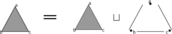
Figure. 1: A subanalytic stratification of a closed triangle $Z$.

Our interest is in $Z\subset\mathbb{R}^{n}$ which is a compact subanalytic set with $\dim_{\mathbb{R}}Z<n$. It follows from Theorem A in [7] that there exists a subanalytic stratification $\{Z_{\alpha}\}_{\alpha\in\Lambda}$ where each stratum $Z_{\alpha}$ is an L-regular s-cell. See 6. Definition in [7] for the definition of an L-regular s-cell. Furthermore, since $Z$ is compact, the subanalytic stratum $\{Z_{\alpha}\}_{\alpha\in\Lambda}$ of $Z$ is locally finite in $X$ implying that the index set $\Lambda$ is finite.

The properties of the L-regular s-cell $Z_{\alpha}$ ($\alpha\in\Lambda$) that we need are that it can be built up from a zero or one dimensional set $B_{1}$, using orthogonal coordinates $(x_{1},...,x_{n})\in\mathbb{R}^{n}$, a positive constant $M$, and where the build up is through ordered pairs $(B_{k},\Phi_{k})$, $(k=1,...,n-1)$, referred to as data, where $B_{k}\subset\mathbb{R}^{k}$ and $\Phi_{k}$ is a set of functions whose details are given below. The stratum, $Z_{\alpha}$, is thus a kind of cylinder cell built up from a lower dimensional cell to a higher dimensional one; see Figure 2.

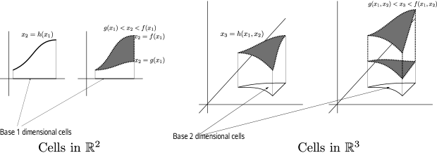
Figure. 2: A cylinder cell built up from a base one.

Properties of the L-regular s-cell $Z_{\alpha}$

1. The set $B_{1}$ is a point or an open interval in $\mathbb{R}^{1}_{x_{1}}$. Each $B_{k}$ is a locally closed subanalytic subset in $\mathbb{R}^{k}_{x_{1},\dots,x_{k}}$ and it is analytic smooth at each point in $B_{k}$.

2. The set $\Phi_{k}$ is a set consisting of one continuous subanalytic function $h_{k}$ on $\overline{B}_{k}$ or two continuous subanalytic functions $f_{k}$ and $g_{k}$ on $\overline{B}_{k}$ with $f_{k}(x^{\prime})>g_{k}(x^{\prime})$ ($x^{\prime}\in B_{k}$). Furthermore, for any $\varphi\in\Phi_{k}$, $\varphi$ is analytic on $B_{k}$ and has the estimate

   $$|d_{B_{k}}\varphi(x^{\prime})|\leq M\qquad(x^{\prime}\in B_{k}).$$ (27)

   Here $d_{B_{k}}\varphi$ denotes the differential 1-form of $\varphi$ on $B_{k}$ and the cotangent bundle of $B_{k}$ is equipped with the metric induced from the standard one in $\mathbb{R}^{k}$.

3. For $k=1,\dots,n-1$, if $\Phi_{k}$ consists of one function, then

   $$B_{k+1}=\{(x^{\prime},x_{k+1})\in\mathbb{R}^{k+1}\,:\,x^{\prime}\in B_{k},\,x_{k+1}=h_{k}(x^{\prime})\},$$

   where $x^{\prime}=(x_{1},\dots,x_{k})$, and otherwise we have

   $$B_{k+1}=\{(x^{\prime},x_{k+1})\in\mathbb{R}^{k+1}\,:\,x^{\prime}\in B_{k},\,g_{k}(x^{\prime})<x_{k+1}<f_{k}(x^{\prime})\}.$$

   Here we set $B_{n}:=Z_{\alpha}$.

Summing up, as Figure 2 shows, the L-regular s-cell $Z_{\alpha}$ is constructed successively from $B_{1}$ to $B_{n}=Z_{\alpha}$ using functions in $\Phi_{1}$, …, $\Phi_{n-1}$. Furthermore $Z_{\alpha}$ itself and each component of $\partial Z_{\alpha}$ are sufficiently flat due to (27).

Our goal is to present a theorem that gives an open covering, whose measure we can estimate, of the zero level set of a subanalytic function. Prior to presenting and proving this theorem we establish that we can extend a function in $\Phi_{k}$ (defined on $\overline{B}_{k}\subset\mathbb{R}^{k}$) to $\mathbb{R}^{k}$ as a subanalytic Lipschitz continuous function. We first establish the following lemma.

Lemma 6.5.

Let $X=\mathbb{R}^{n}$ and $Z$ be a compact subanalytic subset in $X$. Let $\{Z_{\alpha}\}_{\alpha\in\Lambda}$ be a subanalytic stratification of $Z$ with each $Z_{\alpha}$ being an L-regular s-cell. Further, let $\alpha\in\Lambda$ and $\{(B_{k},\Phi_{k})\}_{k=1}^{n-1}$ be the data for $Z_{\alpha}$. Then $\varphi\in\Phi_{k}$ is a Lipschitz continuous function on $\overline{B}_{k}$.

Proof.

If we can show the Lipschitz continuity of $\varphi$ on $B_{k}$, then the claim of the lemma follows from the continuity of $\varphi$ on $\overline{B}_{k}$. Hence it suffices to prove the claim on $B_{k}$. Since $B_{k}$ itself is an L-regular s-cell in $\mathbb{R}^{k}$, by 8. Proposition in [7], there exists a positive constant $C$ for which any points $p$ and $q$ in $B_{k}$ are joined by a smooth curve $\ell$ in $B_{k}$ with

$$\text{the length of $\ell$}\,\leq C|p-q|.$$ (28)

Let $p$ and $q$ be points in $B_{k}$, and let $\ell(s)$ ($0\leq s\leq 1$) be such a curve in $B_{k}$. Then we have

$$|\varphi(p)-\varphi(q)| =\left|\int_{0}^{1}d_{B_{k}}\varphi\left(\frac{d\ell}{ds}(s)\right)ds\right|$$

$$\leq M\int_{0}^{1}\left|\frac{d\ell}{ds}(s)\right|ds=M\times(\text{the length of $\ell$}).$$

Here we identified $\frac{d\ell}{ds}(s)$ with a tangent vector of the manifold $B_{k}$ at $\ell(s)$. Hence the result follows from (28). ∎

Now we construct a family of maps $\rho_{k}:\mathbb{R}^{k}\to\overline{B}_{k}$ ($k=1,2,\dots,n-1$) satisfying the following conditions.

1. $\rho_{k}$ is a subanalytic map on $\mathbb{R}^{k}$ and a Lipschitz continuous map on any compact subset in $\mathbb{R}^{k}$.

2. $\rho_{k}(q)=q$ for $q\in\overline{B}_{k}$.

We construct the family recursively. For $k=1$, we set $\rho(x)=a$ if $B_{1}$ consists of one point $a\in\mathbb{R}$, otherwise we define, for $B_{1}=(a,\,b)\subset\mathbb{R}$ ($a<b$),

$$\rho_{1}(x)=\left\{\begin{aligned} a\qquad&(x<a),\\ x\qquad&(a\leq x\leq b),\\ b\qquad&(b<x).\end{aligned}\right.$$

Clearly the conditions are satisfied for $\rho_{1}$. Suppose that $\rho_{k}$ has been constructed. We first define $\rho^{(1)}_{k+1}:\mathbb{R}^{k+1}\to\overline{B}_{k}\times\mathbb{R}_{x_{k+1}}$ by

$$\rho^{(1)}_{k+1}(x^{\prime},x_{k+1})=(\rho_{k}(x^{\prime}),x_{k+1}),$$

which is subanalytic and Lipschitz continuous by the induction hypothesis.

Now we define $\rho^{(2)}_{k+1}:\overline{B}_{k}\times\mathbb{R}_{x_{k+1}}\to\overline{B}_{k+1}$ in the following way. If $\Phi_{k}$ consists of one function $h_{k}$, we set

$$\rho^{(2)}_{k+1}(x^{\prime},x_{k+1})=(x^{\prime},h_{k}(x^{\prime})).$$

Otherwise we set

$$\rho^{(2)}_{k+1}(x^{\prime},x_{k+1})=\left\{\begin{aligned} (x^{\prime},g_{k}(x^{\prime}))\qquad&(x_{k+1}<g_{k}(x^{\prime})),\\ (x^{\prime},x_{k+1})\qquad&(g_{k}(x^{\prime})\leq x_{k+1}\leq f_{k}(x^{\prime})),\\ (x^{\prime},f_{k}(x^{\prime}))\qquad&(f_{k}(x^{\prime})<x_{k+1}).\end{aligned}\right.$$

Since $h_{k}$ and $f_{k}$, $g_{k}$ are subanalytic and Lipschitz continuous, $\rho^{(2)}_{k+1}$ also becomes a subanalytic and Lipschitz continuous map in both cases. We set $\rho_{k+1}:=\rho^{(2)}_{k+1}\circ\rho^{(1)}_{k+1}$. Then $\rho_{k+1}$ is a subanalytic and Lipschitz continuous map as a composition of maps that have the same properties, and $\rho_{k+1}(q)=q$ for $q\in\overline{B}_{k+1}$ clearly holds by the construction. Hence we have obtained the desired family of maps $\rho_{k}$ $(k=1,\dots,n-1)$.

Let $\varphi\in\Phi_{k}$. Then $\varphi(\rho_{k}(x))$ is a subanalytic and Lipschitz continuous function on $\mathbb{R}^{k}$ and its restriction to $\overline{B}_{k}$ coincides with $\varphi$. Therefore, in what follows, we assume that all the functions belonging to $\Phi_{k}$ are defined in $\mathbb{R}^{k}$ and they are subanalytic and Lipschitz continuous there for any $k=1,2,\dots,n-1$.

It follows from $\operatorname{dim}_{\mathbb{R}}Z_{\alpha}<n$ that there exists $1\leq\kappa\leq n-1$ such that $\Phi_{\kappa}$ consists of only one function $h_{\kappa}$. In fact, otherwise, the $Z_{\alpha}$ becomes an open subset in $X$ which contradicts $\operatorname{dim}_{\mathbb{R}}Z_{\alpha}<n$. Let $\kappa_{\alpha}$ be the largest one of those $\kappa$’s. Then we define the subanalytic open subset $U_{\alpha}(\eta)$ ($\eta>0$) by

$$U_{\alpha}(\eta)=\{x\in\mathbb{R}^{n}\,: h_{\kappa_{\alpha}}(x_{1},\dots,x_{\kappa_{\alpha}})-\eta<x_{\kappa_{\alpha}+1}<h_{\kappa_{\alpha}}(x_{1},\dots,x_{\kappa_{\alpha}})+\eta,$$ (29)

$$\qquad|x_{j}|<R\,\,(j=1,\dots,\kappa_{\alpha},\kappa_{\alpha+2},\dots,n)\}.$$

Clearly $U_{\alpha}(\eta)$ ($\eta>0$) is an open subanalytic subset and it contains $Z_{\alpha}$. For the other $\alpha\in\Lambda$, we can construct a subanalytic open neighborhood $U_{\alpha}(\eta)$ of $Z_{\alpha}$ in the same way.

By setting $U(\eta)=\underset{\alpha\in\Lambda}{\bigcup}U_{\alpha}(\eta)$ with $U_{\alpha}(\eta)$ defined in the above paragraph, we have the following covering theorem.

Theorem 6.6.

Let $Z$ be a compact subanalytic subset in $X$ with $\operatorname{dim}_{\mathbb{R}}Z<n$. Then there exists a family $U(\eta)$ $($$0<\eta\leq 1$$)$ of subanalytic open neighborhoods of $Z$ and positive constants $C_{1}$, $C_{2}$ for which we have the following.

1. $\operatorname{vol}(U(\eta))\leq C_{1}\eta$ for any $\eta\in(0,\,1]$.

2. $\operatorname{dist}(p,\,Z)\geq C_{2}\eta$ for any point $p\in X\setminus U(\eta)$ and any $\eta\in(0,\,1]$.

Proof.

We will establish that $U(\eta)$ has the desired properties described in the statement of the theorem. Since each $U_{\alpha}(\eta)$ is subanalytic open and contains $Z_{\alpha}$, their union $U(\eta)$ becomes a subanalytic open neighborhood of $Z$. The first claim 1. of the theorem is easily seen. In fact, we have

$$\operatorname{vol}(U_{\alpha}(\eta))=\int_{-R}^{R}\dots\int_{h_{\kappa_{\alpha}}-\eta}^{h_{\kappa_{\alpha}}+\eta}\dots\int_{-R}^{R}dx_{1}\dots dx_{n}=2(2R)^{n-1}\eta.$$

Since the number of the strata is finite, the claim follows from this.

We now establish claim 2. of the theorem. Suppose that the claim were false. Then there exists a sequence $\{\eta_{j}\}$ of positive real numbers in $(0,\,1]$ and points $p_{j}\in X\setminus U(\eta_{j})$ satisfying

$$\frac{\operatorname{dist}(p_{j},\,Z)}{\eta_{j}}\to 0\qquad(j\to\infty).$$ (30)

Note that, since $\operatorname{dist}(p_{j},\,Z)\to 0$ ($j\to\infty$) also holds, the sequence $\{p_{j}\}$ is bounded. Hence, by taking a subsequence, we may assume $\eta_{j}\to\eta_{\infty}$ and $p_{j}\to p_{\infty}$ ($j\to\infty$) for some $\eta_{\infty}\in[0,1]$ and $p_{\infty}\in Z$. Suppose $\eta_{\infty}>0$. Then $p_{\infty}$ belongs to both $X\setminus U\left(\dfrac{\eta_{\infty}}{2}\right)$ and $Z$. This contradicts the fact that $U\left(\dfrac{\eta_{\infty}}{2}\right)$ is an open neighborhood of the compact set $Z$. Therefore we assume $\eta_{\infty}=0$, i.e., $\eta_{j}\to 0$ ($j\to\infty$) in what follows.

Let $q_{j}$ be a point in $Z$ with $\operatorname{dist}(p_{j},\,Z)=|p_{j}-q_{j}|$. By taking a subsequence, we may assume $q_{j}\in Z_{\alpha}$ ($j=1,2,\dots$) for some $\alpha$. Let $\pi_{k}:\mathbb{R}^{n}\to\mathbb{R}^{k}$ ($k=1,2,\dots,n$) denote the canonical projection defined by

$$\pi_{k}(x_{1},\dots,x_{n})=(x_{1},\dots,x_{k}).$$

Let $\kappa_{\alpha}$ be the index determined before equation (29). Then we have

$${}|\pi_{\kappa_{\alpha}}(p_{j})-\pi_{\kappa_{\alpha}}(q_{j})|\leq\operatorname{dist}(p_{j},\,Z)$$ (31)

and

$${}|\pi_{\kappa_{\alpha}+1}(p_{j})-\pi_{\kappa_{\alpha}+1}(q_{j})|\leq\operatorname{dist}(p_{j},\,Z).$$ (32)

Note that, since $q_{j}\in Z_{\alpha}$ and $\Phi_{\kappa_{\alpha}}$ consists of only one function $h_{\kappa_{\alpha}}$, it follows from the construction of $Z_{\alpha}$ described above that the relation

$$\pi_{\kappa_{\alpha}+1}(q_{j})=(\pi_{\kappa_{\alpha}}(q_{j}),\,h_{\kappa_{\alpha}}(\pi_{\kappa_{\alpha}}(q_{j})))\in\mathbb{R}^{\kappa_{\alpha}+1}$$

holds.

Set $\tilde{p}_{j}=(\pi_{\kappa_{\alpha}}(p_{j}),\,h_{\kappa_{\alpha}}(\pi_{\kappa_{\alpha}}(p_{j})))\in\mathbb{R}^{\kappa_{\alpha}+1}.$ Then, as $p_{j}\notin U_{\alpha}(\eta_{j})$ and $\operatorname{dist}(p_{j},\,Z_{\alpha})\to 0$ ($j\to\infty$), we have

$${}|\tilde{p}_{j}-\pi_{\kappa_{\alpha}+1}(p_{j})|\geq\eta_{j}$$ (33)

for sufficiently large $j$’s. Since the function $h_{\kappa_{\alpha}}$ is Lipschitz continuous, we also have

$$|h_{\kappa_{\alpha}}(\pi_{\kappa_{\alpha}}(p_{j}))-h_{\kappa_{\alpha}}(\pi_{\kappa_{\alpha}}(q_{j}))| \leq L|\pi_{\kappa_{\alpha}}(p_{j})-\pi_{\kappa_{\alpha}}(q_{j})|$$ (34)

$$\leq L\operatorname{dist}(p_{j},\,Z)$$

for a positive constant $L$. Therefore, by (31) and (34), we obtain

$${}|\tilde{p}_{j}-\pi_{\kappa_{\alpha}+1}(q_{j})|=\left|(\pi_{\kappa_{\alpha}}(p_{j}),\,h_{\kappa_{\alpha}}(\pi_{\kappa_{\alpha}}(p_{j})))-(\pi_{\kappa_{\alpha}}(q_{j}),\,h_{\kappa_{\alpha}}(\pi_{\kappa_{\alpha}}(q_{j})))\right|\leq(1+L)\operatorname{dist}(p_{j},\,Z).$$ (35)

Summing up, by (32), (33) and (35), we get

$$\eta_{j}\leq|\tilde{p}_{j}-\pi_{\kappa_{\alpha}+1}(p_{j})| \leq|\tilde{p}_{j}-\pi_{\kappa_{\alpha}+1}(q_{j})|+|\pi_{\kappa_{\alpha}+1}(q_{j})-\pi_{\kappa_{\alpha}+1}(p_{j})|$$

$$\leq(2+L)\operatorname{dist}(p_{j},\,Z),$$

from which we have

$$1\leq(2+L)\frac{\operatorname{dist}(p_{j},\,Z)}{\eta_{j}}.$$

This contradicts (30) if $j$ tends to $\infty$, and hence, the claim 2. must be true. The proof has been completed. ∎

Proposition 6.7.

Let $\Omega$ be a relatively compact open subanalytic subset in $\mathbb{R}^{n}$ and $f$ a real valued continuous subanalytic function on $\overline{\Omega}$. Suppose that there exists a subanalytic stratification $\{\Omega_{\alpha}\}_{\alpha\in\Lambda}$ of $\overline{\Omega}$ such that $f|_{\Omega_{\alpha}}$ is analytic in $\Omega_{\alpha}$ and analytically extends to an open neighborhood of $\overline{\Omega}_{\alpha}$ for any $\alpha\in\Lambda$ with $\operatorname{dim}_{\mathbb{R}}\Omega_{\alpha}=n$. Then there exists a finite subset $E$ of $\mathbb{R}$ and a positive constant $M_{f}$ satisfying

$$H_{n-1}\left(\left\{x\in\overline{\Omega}\,:\,f(x)=t\right\}\right)\leq M_{f}$$

for any $t\in\mathbb{R}\setminus E$. Furthermore, let $Z$ be a closed subanalytic subset in $\overline{\Omega}$ with $\operatorname{dim}_{\mathbb{R}}Z\leq n-2$. Then

$$\sup_{t\in\mathbb{R}\setminus E}H_{n-1}\left(\left\{x\in\overline{\Omega}\cap Z_{\epsilon}\,:\,f(x)=t\right\}\right)\to 0\qquad(\epsilon\to 0^{+}).$$

Here $Z_{\epsilon}:=\{x\in\overline{\Omega},\,:\,\operatorname{dist}(x,Z)\leq\epsilon\}$.

Remark: If $f$ is $C^{\infty}$, i.e., without subanalyticity, then the claim in the proposition does not hold even if a subset of measure zero is allowed as $E$.

Proof.

For any $t\in\mathbb{R}$, we set $S_{t}:=\{x\in\overline{\Omega}\,:\,f(x)=t\}$. As we have

$$\overline{\Omega}=\underset{\alpha\in\Lambda,\,,\operatorname{dim}_{\mathbb{R}}\Omega_{\alpha}=n}{\cup}\overline{\Omega}_{\alpha}$$

and $\Lambda$ is a finite set, it suffices to show the corresponding claim on $\overline{\Omega}_{\alpha}$ for each $\alpha$ with $\operatorname{dim}_{\mathbb{R}}\Omega_{\alpha}=n$. Hence, in what follows, we assume that $f$ is analytic in $\Omega$ and analytically extendable to an open neighborhood of $\overline{\Omega}$. If $f$ is a constant function $c$ in $\Omega$, then we take $E=\{c\}$, for which the claim clearly holds. Therefore we may assume that $f$ is not constant and, as a result, we have $\operatorname{dim}_{\mathbb{R}}S_{t}<n$ for any $t$.

Set $\overline{\Omega}_{sing}:=\{x\in\overline{\Omega}\,:\,|\nabla f(x)|=0\}$ and $\overline{\Omega}_{reg}:=\overline{\Omega}\setminus\overline{\Omega}_{sing}$. Then $f(\overline{\Omega}_{sing})$ is a subanalytic subset in $\mathbb{R}$ as $f$ is proper on $\overline{\Omega}$ and it is a measure-zero set by Sard’s theorem. Hence $f(\overline{\Omega}_{sing})$ consists of finite points in $\mathbb{R}$ and we take it as $E$.

Let $p_{k}:\mathbb{R}^{n}\to\mathbb{R}^{n-1}$ be the canonical projection by excluding the coordinate $x_{k}$. We set

$$\overline{\Omega}_{k}:=\left\{x\in\overline{\Omega}_{reg}\,:\,|\nabla f(x)-\langle\nabla f(x),\,e_{k}\rangle e_{k}|\leq n|\langle\nabla f(x),\,e_{k}\rangle|\right\},$$

where $e_{k}$ is the unit vector with its $k$-th component being $1$. Note that $\overline{\Omega}_{k}$ is subanalytic in $\mathbb{R}^{n}$ and $\overline{\Omega}_{reg}=\cup_{1\leq k\leq n}\Omega_{k}$ holds. Furthermore we set

$$S_{t,k}:=S_{t}\cap\overline{\Omega}_{k},$$

which is also subanalytic in $\mathbb{R}^{n}$. Then, for any $t\in\mathbb{R}\setminus E$, since $|\nabla f(x)|\neq 0$ on $S_{t}$, we have $S_{t}=\cup_{1\leq k\leq n}S_{t,k}$ and $S_{t,k}$ is an analytic smooth hypersurface in $\overline{\Omega}_{k}$. By these observations it suffices to show $\underset{t\in\mathbb{R}\setminus E}{\max}\,H_{n-1}(S_{t,k})<+\infty$.

Define

$$\ell_{1} :=\underset{x^{\prime}\in p_{k}(\overline{\Omega}_{k})}{\max}\#\left(\overline{\Omega}_{k}\cap p_{k}^{-1}(x^{\prime})\right),$$

$$\ell_{2} :=\underset{x^{\prime}\in p_{k}(\overline{\Omega}_{k})}{\max}\#\left\{x\in\overline{\Omega}\cap p_{k}^{-1}(x^{\prime})\,:\,\dfrac{\partial f}{\partial x_{k}}(x)=0\right\},$$

where $\#A$ denotes the number of the connected components of a set $A$. Note that these numbers certainly exist because the direct images $p_{k\,*}\mathbb{R}_{\overline{\Omega}_{k}}$ and $p_{k\,*}\mathbb{R}_{\{x\in\overline{\Omega}\,:\,f_{x_{k}}(x)=0\}}$ of constructible sheaves $\mathbb{R}_{\overline{\Omega}_{k}}$ and $\mathbb{R}_{\{x\in\overline{\Omega}\,:\,f_{x_{k}}(x)=0\}}$ are again constructible sheaves by Proposition 8.4.8 ([6]) and

$$\dim_{\mathbb{R}}\left(p_{k\,*}\mathbb{R}_{\overline{\Omega}_{k}}\right)_{x^{\prime}} =\#\left(\overline{\Omega}_{k}\cap p_{k}^{-1}(x^{\prime})\right),$$

$$\dim_{\mathbb{R}}\left(p_{k\,*}\mathbb{R}_{\{x\in\overline{\Omega}\,:\,f_{x_{k}}(x)=0\}}\right)_{x^{\prime}} =\#\left\{x\in\overline{\Omega}\cap p_{k}^{-1}(x^{\prime})\,:\,\dfrac{\partial f}{\partial x_{k}}(x)=0\right\},$$

hold for $x^{\prime}\in p_{k}(\overline{\Omega}_{k})$ (see also Chapter VIII in ([6]) for the definition of a constructible sheaf).

As $p_{k}:S_{t,k}\to p_{k}(S_{t,k})$ is a finite map, that is, $p_{k}|_{S_{t,k}}$ is a proper map and $p_{k}^{-1}(x^{\prime})\cap S_{t,k}$ consists of finite points for every $x^{\prime}\in p_{k}(S_{t,k})$, there exists a subanalytic stratification $\{O_{\beta}\}_{\beta\in\Xi}$ of $p_{k}(S_{t,k})$ such that $S_{t,k}\cap p^{-1}_{k}(O_{\beta})$ becomes a finite covering over $O_{\beta}$ for each $\beta$. Note that the stratification consists of a finite number of strata.

Furthermore the number of connected components of $S_{t,k}\cap p^{-1}_{k}(O_{\beta})$ is at most $\ell_{1}+\ell_{2}$, which can be proved as follows: As $O_{\beta}$ is connected, it suffices to show that the number of points $p^{-1}_{k}(x^{\prime})\cap S_{t,k}$ ($x^{\prime}\in O_{\beta}$) is at most $\ell_{1}+\ell_{2}$. Let $L$ be the line $p^{-1}_{k}(x^{\prime})$. We first assume that $L\cap\overline{\Omega}_{k}$ is connected, i.e., $\ell_{1}=1$. Then there exist mutually distinct points $q_{1},\dots,q_{m}$ in $L$ such that, in each open interval $(q_{k},\,q_{k+1})$ of $L$, $f(x)$ is strictly increasing, strictly decreasing or constant. As $S_{t,k}$ intersects $L$ transversally, $S_{t,k}$ never intersects an interval where $f(x)$ is constant. Since the number of intervals in which $f(x)$ is non-constant is at most $\ell_{2}+1$ and since $S_{t,k}$ intersects the closure of such an interval at one point if exists, we conclude that $S_{t,k}\cap L$ consists of at most $\ell_{2}+1=\ell_{1}+\ell_{2}$ points. By applying the same argument to each connected component of $L\cap\overline{\Omega}_{k}$, we can prove the claim for the case $\ell_{1}>1$.

For $\beta$ with $\operatorname{dim}_{\mathbb{R}}O_{\beta}<n-1$, since $p_{k}|_{S_{t,k}}$ is a finite covering over $O_{\beta}$, we have

$$\operatorname{dim}_{\mathbb{R}}(S_{t,k}\cap p^{-1}_{k}(O_{\beta}))<n-1,$$

which implies $H_{n-1}(S_{t,k}\cap p^{-1}_{k}(O_{\beta}))=0$. On the other hand, for $\beta$ with $\operatorname{dim}_{\mathbb{R}}O_{\beta}=n-1$, we have

$$H_{n-1}(S_{t,k}\cap p^{-1}_{k}(O_{\beta}))\leq\sqrt{1+n^{2}}(\ell_{1}+\ell_{2})H_{n-1}(O_{\beta}).$$

Hence we have

$$H_{n-1}(S_{t,k}) \leq\sqrt{1+n^{2}}(\ell_{1}+\ell_{2})\sum_{\beta\in\Xi\,:\,\operatorname{dim}_{\mathbb{R}}O_{\beta}=n-1}H_{n-1}(O_{\beta})$$ (36)

$$\leq\sqrt{1+n^{2}}(\ell_{1}+\ell_{2})H_{n-1}(p_{k}(\overline{\Omega})).$$

This shows the first claim of the proposition.

Finally we show the last claim. Clearly $\dim_{\mathbb{R}}p_{k}(Z)<n-1$ and

$$p_{k}(Z_{\epsilon})\subset\left(p_{k}(Z)\right)_{\epsilon}:=\{y\in\mathbb{R}^{n-1}\,:\,\operatorname{dist}(y,p_{k}(Z))\leq\epsilon\}$$

hold. Hence we have, in $\mathbb{R}^{n-1}$,

$$0\leq H_{n-1}\left(p_{k}(Z_{\epsilon})\right)\leq H_{n-1}\left(\left(p_{k}(Z)\right)_{\epsilon}\right)\to 0,\qquad(\epsilon\to 0^{+})$$

due, for example, to the second Theorem in this Appendix. Then the last claim of the proposition immediately follows from (36). ∎

References

[1]
G. Alessandrini, An identification problem for an elliptic equation in two variables, Ann. Mat. Pura Appl., 145(1986)265-296.
[2]
G. Bal and G. Uhlmann, Reconstructions for some coupled-physics inverse problems, Applied Math. Letters (2012) doi:10.1016/j.aml.2012.03.005
[3]
G. Bal and G. Uhlmann, Reconstruction of coefficients in scalar second-order elliptic equations from knowledge of their solutions (2012), preprint
[4]E. Bierstone and P. D. Milman,
Semianalytic and subanalytic sets,
Inst. Hautes Études Sci. Publ. Math., 67, (1988) 5-42
[5]
L. Evans and R. Gareipy, Measure Theory and Fine Properties of Functions, CRC Press, Boca Raton,1992.
[6] M. Kashiwara and P. Schapira, Sheaves on manifolds,
Grundlehren der mathematischen Wissenschaften. Vol. 292, Sprinter, Berlin, 1990.
[7] K. Kurdyka,
On a subanalytic stratification satisfying a Whitney property with exponent,
Real algebraic geometry (Rennes, 1991),
Lecture Notes in Math. 1524,
Springer, Berlin,
(1992) 316-322.
[8]
R. Muthupillai, D. Lomas, R. Rossman, J. Greenlead, A. Manduca, and R. Ehman, Magnetic resonance elastography by direct visualization of propagating acoustic strain waves, Science, 269 (1995) 1854–1857.
[9]
G. Nakamura, Y. Jiang, S. Nagayasu and J. Cheng, Inversion analysis for magnetic resonance elastography, Appl. Anal., 87(2008)165-179.
[10]
G. Richter, An inverse problem for the steady state diffusion equation, SIAM J. Appl. Math., 41(1981) 210-221.
[11]
F. Treves, Introduction to pseudodifferential and Fourier integral operators. Vol. 1, 2, Plenum Press, New York-London, 1980.
[12]
M. Yin, J. Talwalkar, K. Glaser, and R. Ehman, MR Elastography of the Liver: Observations from a Review of 1,377 Exams,
ISMRM 19th Annual Meeting www.ismrm.org/11/Session39.htm.
[13]
K. Lin, J. McLaughlin, N. Zhang, ”Log-elastographic and non-marching full inversion schemes for shear modulus recovery from single frequency elastographic data”, Inverse Problems, Vol 25(7), July, 2009.