Cosmological Tests Using GRBs, the Star Formation Rate
and Possible Abundance Evolution

Abstract

The principal goal of this paper is to use attempts at reconciling the Swift long gamma-ray bursts (LGRBs) with the star formation history (SFH) to compare the predictions of $\Lambda$CDM with those in the $R_{\rm h}=ct$ Universe. In the context of the former, we confirm that the latest Swift sample of GRBs reveals an increasing evolution in the GRB rate relative to the star formation rate (SFR) at high redshifts. The observed discrepancy between the GRB rate and the SFR may be eliminated by assuming a modest evolution parameterized as $(1+z)^{0.8}$—perhaps indicating a cosmic evolution in metallicity. However, we find a higher metallicity cut of $Z=0.52Z_{\odot}$ than was seen in previous studies, which suggested that LGRBs occur preferentially in metal poor environments, i.e., $Z\sim 0.1-0.3Z_{\odot}$. We use a simple power-law approximation to the high-z ($\ga 3.8$) SFH, i.e., $R_{\rm SF}\propto[(1+z)/4.8]^{\alpha}$, to examine how the high-z SFR may be impacted by a possible abundance evolution in the Swift GRB sample. For an expansion history consistent with $\Lambda$CDM, we find that the Swift redshift and luminosity distributions can be reproduced with reasonable accuracy if $\alpha=-2.41_{-2.09}^{+1.87}$. For the $R_{\rm h}=ct$ Universe, the GRB rate is slightly different from that in $\Lambda$CDM, but also requires an extra evolutionary effect, with a metallicity cut of $Z=0.44Z_{\odot}$. Assuming that the SFR and GRB rate are related via an evolving metallicity, we find that the GRB data constrain the slope of the high-z SFR in $R_{\rm h}=ct$ to be $\alpha=-3.60_{-2.45}^{+2.45}$. Both cosmologies fit the GRB/SFR data rather well. However, in a one-on-one comparison using the Aikake Information Criterion, the best-fit $R_{\rm h}=ct$ model is statistically preferred over the best-fit $\Lambda$CDM model with a relative probability of $\sim 70\;\%$ versus $\sim 30\;\%$.

1 Introduction

Our understanding of the star formation history (SFH) in the Universe continues to be refined with improving measurement techniques and a broader coverage in redshift—now extending out to $z\ga 6$. However, direct star formation rate (SFR) measurements are quite challenging at these high redshifts, particularly towards the faint end of the galaxy luminosity function. Using ultraviolet and far-infrared observations, Hopkins & Beacom (2006) constrained the cosmic SFH out to $z\approx 6$, and found that the SFR rapidly increases at $z\la 1$, remains almost constant in the redshift range $1\la z\la 4$, and then shows a steep decline with slope $\sim-8$ at $z\ga 4$. The sharp drop at $z\ga 4$ may be due to significant dust extinction at such high redshifts. Li (2008) derived the SFR out to $z=7.4$ by adding new ultraviolet measurements and obtained a shallower decay ($\sim-4.46$) in this range. The high-z SFR has also been constrained using observations of color-selected Lyman break galaxies (LBG; Bouwens et al. 2008; Mannucci et al. 2007; Verma et al. 2007) and Ly$\alpha$ Emitters (LAE; Ota et al. 2008). Several of the more prominent SFR determinations are summarized in Figure 1 below. One can see from this plot that, due to the inherent difficulty of making and interpreting these measurements, the various determinations can disagree with each other even after taking the uncertainties into account.

Gamma-ray bursts (GRBs) are the most luminous transient events in the cosmos. Owing to their high luminosity, GRBs can be detected out to the edge of the visible Universe, constituting a powerful tool for probing the cosmic star formation rate from a different perspective, i.e., by studying the death rate of massive stars rather than observing them directly during their lives. Since the successful launch of the Swift satellite, the number of measured GRB redshifts has increased rapidly, and thus a reliable statistical analysis is now possible. The statistical analysis on the GRB redshift distributions have been well investigated (e.g. Shao et al. 2011; Robertson & Ellis 2012; Dado & Dar 2013). It is believed that long bursts (LGRBs) with durations $T_{\rm 90}>2$ s (where $T_{\rm 90}$ is the time over which $90\%$ of the prompt emission was observed; Kouveliotou et al. 1993) are powered by the core collapse of massive stars (e.g., Woosley 1993a; Paczynski 1998; Woosley & Bloom 2006), an idea given strong support by several confirmed associations between LGRBs and supernovae (Stanek et al. 2003; Hjorth et al. 2003; Chornock et al. 2010).

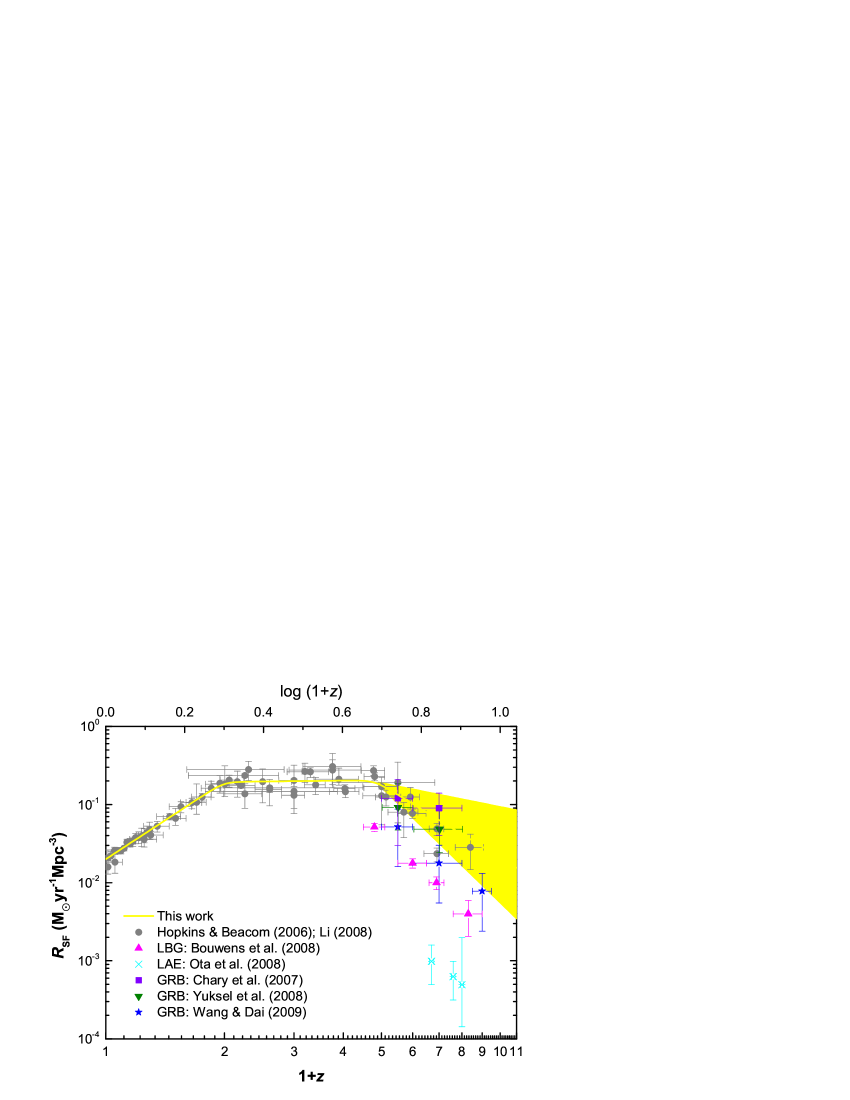
Figure 1: The cosmic star formation rate as a function of redshift. The high-z SFR (shaded band) is constrained by the Swift GRB data, and is characterized by a power-law index $-5.07<\alpha<-1.05$ (see § 4.2). Some observationally-determined SFRs are also shown for comparison.

This scenario—known as the collapsar model—suggests that the cosmic GRB rate should in principle trace the cosmic star formation rate (Totani 1997; Wijers et al. 1998; Blain & Natarajan 2000; Lamb & Reichart 2000; Porciani & Madau 2001; Piran 2004; Zhang & Mészáros 2004; Zhang 2007). However, observations seem to indicate that the rate of LGRBs does not strictly follow the SFR, but instead increases with cosmic redshift faster than the SFR, especially at high-z (Daigne et al. 2006; Le & Dermer 2007; Yüksel & Kistler et al. 2007; Salvaterra & Chincarini 2007; Guetta & Piran 2007; Li 2008; Kistler et al. 2008; Salvaterra et al. 2009, 2012). This has led to the introduction of several possible mechanisms that could produce such an observed enhancement to the GRB rate (Daigne et al. 2006; Guetta & Piran 2007; Le & Dermer 2007; Salvaterra & Chincarini 2007; Kistler et al. 2008, 2009; Li 2008; Salvaterra et al. 2009, 2012; Campisi et al. 2010; Qin et al. 2010; Wanderman & Piran 2010; Cao et al. 2011; Virgili et al. 2011; Robertson & Ellis 2012; Elliott et al. 2012). The idea that appears to have gained some traction is the possibility that the difference between the GRB rate and the SFR is due to an enhanced evolution parameterized as $(1+z)^{\delta}$ (Kistler et al. 2008), which may encompass the effects of cosmic metallicity evolution (Langer & Norman 2006; Li 2008), an evolution in the stellar initial mass function (Xu & Wei 2009; Wang & Dai 2011), and possible selection effects (see, e.g., Coward et al. 2008, 2013; Lu et al. 2012).

Of course, if we knew the mechanism responsible for the difference between the GRB rate and the SFR, we could constrain the high-z SFR very accurately using the GRB data alone. This limitation notwithstanding, GRBs have indeed already been used to estimate the SFR in several instances, including the following representative cases: Chary et al. (2007) estimated a lower limit to the SFR of $0.12\pm 0.09$ and $0.09\pm 0.05$ $M_{\bigodot}$ $\rm yr^{-1}$ $\rm Mpc^{-3}$ at $z=4.5$ and $6$, respectively, using deep observations of three $z\sim 5$ GRBs with the Spitzer Space Telescope; Yüksel et al. (2008) used Swift GRB data to constrain the SFR in the range $z=4-7$ and found that no steep drop exists in the SFR up to at least $z\sim 6.5$; Kistler et al. (2009) constrained the SFR using four years of Swift observations and found that the SFR to $z\ga 8$ was consistent with LBG-based measurements; Wang & Dai (2009) studied the high-z SFR up to $z\sim 8.3$, but found that the SFR at $z\ga 4$ showed a steep decay with a slope of $\sim-5.0$; and Ishida et al. (2011) used the principal component analysis method to measure the high-z SFR from the GRB data and found that the level of star formation activity at $z\approx 4$ could have been already as high as the present-day one ($\approx 0.01$ $M_{\bigodot}$ $\rm yr^{-1}$ $\rm Mpc^{-3}$).

The question of how the GRB redshift distribution is related to the SFH is clearly still not completely answered, but there is an additional important ingredient that has hitherto been ignored in this ongoing discussion—the impact on this relationship from the assumed cosmological expansion itself. Our principal goal in this paper is to update and enlarge the GRB sample using the latest catalog of 254 Swift LGRBs in order to carry out a comparative analysis between $\Lambda$CDM and the $R_{\rm h}=ct$ Universe. We wish to examine the influence on these results due to the background cosmology, and see to what extent the implied abundance evolution depends on the expansion scenario. We will assemble our sample in § 2, and discuss our method of analysis in § 3. A possible mechanism of evolution and the implied high-z SFR are investigated in § 4, together with a direct comparison between the two cosmologies. Our discussion and conclusions are presented in § 5.

2 The Swift GRB observations

Swift has enabled observers to greatly extend the reach of GRB measurements relative to the pre-Swift era, resulting in the creation of a rich data set. To obtain reliable statistics, we consider long bursts detected by Swift up to July, 2013, with accurate redshift measurements and durations exceeding $T_{\rm 90}>2$ s. We calculate the isotropic-equivalent luminosity of a GRB using

$$L_{\rm iso}={E_{\rm iso}(1+z)\over T_{\rm 90}}\;,$$ (1)

where $E_{\rm iso}$ is the rest-frame isotropic equivalent $1-10^{4}$ keV gamma-ray energy. The low-luminosity ($L_{\rm iso}<10^{49}$ erg $\rm s^{-1}$) GRBs are not included in our sample because they may belong to a distinct population (Soderberg et al. 2004; Cobb et al. 2006; Liang et al. 2007; Chapman et al. 2007).

With these criteria, we combine the samples presented in Butler et al. (2007, 2010), Perley et al. (2009), Sakamoto et al. (2011), Greiner et al. (2011), Kr$\ddot{\rm u}$hler et al. (2011), Hjorth et al. (2012), and Perley & Perley (2013). For GRBs where the samples disagree, we choose the most recently measured redshifts. The combined catalog containts 258 GRBs with known redshifts and redshift upper limits, but four GRBs (051002, 051022, 060505, and 071112C) have incomplete fluence or burst duration measurements and are discarded. The remaining 254 long duration GRBs with redshifts or redshift limits serve as our base GRB catalog. Our final sample is listed in Table 1, which includes the following information for each GRB: (1) its name; (2) the redshift $z$; (3) the burst duration $T_{\rm 90}$; and (4) the isotropic-equivalent energy $E_{\rm iso}$. The quantities $T_{\rm 90}$ and $E_{\rm iso}$ of 231 GRBs are directly taken from the catalog of Butler et al. (2007, 2010) and those of 14 others (050412, 050607, 050713A, 060110, 060805A, 060923A, 070521, 071011, 080319A, 080320, 080516, 081109, 081228, and 090904B) are from Robertson & Ellis (2012). The duration $T_{\rm 90}$ of the nine remaining GRBs (050406, 050502B, 051016B, 060602A, 070419B, 080325, 090404, 090417B, and 090709A) are taken from Sakamoto et al. (2011), while their isotropic energy $E_{\rm iso}$ is calculated from the 15 to 150 keV fluences reported by Sakamoto et al. (2011); we correct the observed fluence in a given bandpass to the cosmological rest frame ($1-10^{4}$ keV in this analysis).

Table 1: GRB Catalog.

GRB	z	$T_{90}$	log $E_{\rm iso}^{\Lambda{\rm CDM}}$	log ${E}_{\rm iso}^{R_{\rm h}=ct}$	GRB	z	$T_{90}$	log $E_{\rm iso}^{\Lambda{\rm CDM}}$	log ${E}_{\rm iso}^{R_{\rm h}=ct}$
		(s)	(erg)	(erg)			(s)	(erg)	(erg)
130701A	1.155	4.62 $\pm$ 0.09	$52.32^{+0.07}_{-0.03}$	$52.23\par^{+0.07}_{-0.03}$	080520	1.545	2.97 $\pm$ 0.24	$51.05^{+\par 5.78}_{-0.16}$	$50.96^{+5.78}_{-0.16}$
130612A	2.006	6.64 $\pm$ 1.06	$51.70^{+0.31}_{-0.09}$	$51.62\par^{+0.31}_{-0.09}$	080516	$3.6^{a}$	$5.75^{b}$	$53.08^{+\par 0.22}_{-0.17}$c	$53.04^{+0.22}_{-0.17}$
130610A	2.092	48.45 $\pm$ 2.35	$52.71^{+0.44}_{-0.10}$	$52.63\par^{+0.44}_{-0.10}$	080430	0.767	16.20 $\pm$ 0.78	$51.60^{+\par 0.34}_{-0.09}$	$51.51^{+0.34}_{-0.09}$
130606A	5.913	278.52 $\pm$ 3.54	$53.39^{+0.36}_{-0.08}$	$53.39\par^{+0.36}_{-0.08}$	080413B	1.1	7.04 $\pm$ 0.43	$52.20^{+\par 0.06}_{-0.05}$	$52.10^{+0.06}_{-0.05}$
130604A	1.06	78.07 $\pm$ 9.81	$51.90^{+0.50}_{-0.09}$	$51.81\par^{+0.50}_{-0.09}$	080413A	2.433	46.62 $\pm$ 0.13	$52.97^{+\par 0.30}_{-0.08}$	$52.90^{+0.30}_{-0.08}$
130603B	0.3564	2.20 $\pm$ 0.01	$50.89^{+0.66}_{-0.15}$	$50.83\par^{+0.66}_{-0.15}$	080411	1.03	58.29 $\pm$ 0.46	$53.38^{+\par 0.17}_{-0.08}$	$53.28^{+0.17}_{-0.08}$
130514A	3.6	220.32 $\pm$ 5.60	$53.60^{+0.12}_{-0.05}$	$53.55\par^{+0.12}_{-0.05}$	080330	1.51	66.10 $\pm$ 0.98	$51.63^{+\par 0.99}_{-0.06}$	$51.54^{+0.99}_{-0.06}$
130511A	1.3033	4.95 $\pm$ 0.82	$51.24^{+0.70}_{-0.14}$	$51.14\par^{+0.70}_{-0.14}$	080325	$1.78^{d}$	$162.82^{e}$	$53.12^{+\par 0.04}_{-0.04}$f	$53.03^{+0.04}_{-0.04}$
130505A	2.27	292.81 $\pm$ 33.84	$54.31^{+0.45}_{-0.23}$	$54.23\par^{+0.45}_{-0.23}$	080320	$7^{g}$	$13.80^{b}$	$53.53^{+\par 0.58}_{-0.07}$c	$53.56^{+0.58}_{-0.07}$
130427B	2.78	7.04 $\pm$ 0.26	$52.50^{+0.39}_{-0.09}$	$52.44\par^{+0.39}_{-0.09}$	080319C	1.95	32.88 $\pm$ 3.27	$52.80^{+\par 0.37}_{-0.09}$	$52.72^{+0.37}_{-0.09}$
130427A	0.3399	324.70 $\pm$ 2.50	$53.66^{+0.19}_{-0.11}$	$53.60\par^{+0.19}_{-0.11}$	080319B	0.937	147.32 $\pm$ 2.50	$54.58^{+\par 0.26}_{-0.17}$	$54.49^{+0.26}_{-0.17}$
130420A	1.297	114.84 $\pm$ 4.84	$52.72^{+0.07}_{-0.05}$	$52.63\par^{+0.07}_{-0.05}$	080319A	$2.2^{g}$	$43.60^{b}$	$53.47^{+\par 0.38}_{-0.06}$c	$53.39^{+0.38}_{-0.06}$
130418A	1.217	97.92 $\pm$ 2.26	$51.77^{+0.14}_{-0.08}$	$51.68\par^{+0.14}_{-0.08}$	080310	2.4266	361.92 $\pm$ 3.75	$52.78^{+\par 0.78}_{-0.07}$	$52.71^{+0.78}_{-0.07}$
130408A	3.758	5.64 $\pm$ 0.31	$53.08^{+0.55}_{-0.13}$	$53.04\par^{+0.55}_{-0.13}$	080210	2.641	43.89 $\pm$ 4.36	$52.72^{+\par 0.39}_{-0.08}$	$52.65^{+0.39}_{-0.08}$
130215A	0.597	89.05 $\pm$ 8.39	$51.89^{+0.31}_{-0.07}$	$51.81\par^{+0.31}_{-0.07}$	080207	2.0858	310.98 $\pm$ 9.34	$53.05^{+\par 0.23}_{-0.07}$	$52.96^{+0.23}_{-0.07}$
130131B	2.539	4.74 $\pm$ 0.21	$52.23^{+0.03}_{-0.03}$	$52.16\par^{+0.03}_{-0.03}$	080129	4.349	45.60 $\pm$ 3.00	$52.90^{+\par 0.42}_{-0.20}$	$52.87^{+0.42}_{-0.19}$
121229A	2.707	26.64 $\pm$ 2.15	$51.85^{+0.95}_{-0.10}$	$51.79\par^{+0.95}_{-0.10}$	071227	0.383	2.20 $\pm$ 0.16	$50.45^{+\par 0.60}_{-0.22}$	$50.39^{+0.60}_{-0.22}$
121211A	1.023	184.14 $\pm$ 2.31	$51.80^{+0.65}_{-0.09}$	$51.70\par^{+0.65}_{-0.09}$	071122	1.14	79.20 $\pm$ 4.88	$51.55^{+\par 0.64}_{-0.14}$	$51.46^{+0.64}_{-0.14}$
121201A	3.385	39.04 $\pm$ 2.93	$52.39^{+0.38}_{-0.08}$	$52.34\par^{+0.38}_{-0.08}$	071117	1.331	6.48 $\pm$ 0.76	$52.29^{+\par 0.18}_{-0.07}$	$52.20^{+0.18}_{-0.07}$
121128A	2.2	25.65 $\pm$ 5.47	$52.98^{+0.10}_{-0.07}$	$52.91\par^{+0.10}_{-0.07}$	071031	2.692	187.18 $\pm$ 7.12	$52.61^{+\par 0.45}_{-0.07}$	$52.54^{+0.45}_{-0.07}$
121027A	1.77	69.30 $\pm$ 1.90	$52.39^{+0.11}_{-0.09}$	$52.31\par^{+0.11}_{-0.09}$	071021	2.145	204.96 $\pm$ 17.95	$53.00^{+\par 0.43}_{-0.14}$	$52.92^{+0.43}_{-0.14}$
121024A	2.298	12.46 $\pm$ 0.39	$52.40^{+0.38}_{-0.16}$	$52.32\par^{+0.38}_{-0.16}$	071020	2.145	4.40 $\pm$ 0.27	$53.00^{+\par 0.43}_{-0.14}$	$52.92^{+0.43}_{-0.14}$
120922A	3.1	179.54 $\pm$ 6.27	$53.28^{+0.21}_{-0.04}$	$53.22\par^{+0.21}_{-0.04}$	071011	$5^{g}$	$80.90^{b}$	$54.37^{+\par 0.34}_{-0.19}$c	$54.36^{+0.34}_{-0.19}$
120909A	3.93	617.70 $\pm$ 30.95	$53.68^{+0.48}_{-0.09}$	$53.64\par^{+0.48}_{-0.09}$	071010B	0.947	34.68 $\pm$ 1.02	$52.26^{+\par 0.09}_{-0.03}$	$52.16^{+0.09}_{-0.03}$
120907A	0.97	6.27 $\pm$ 0.28	$51.29^{+0.40}_{-0.05}$	$51.20\par^{+0.40}_{-0.05}$	071010A	0.98	22.40 $\pm$ 1.70	$51.13^{+\par 0.81}_{-0.07}$	$51.04^{+0.81}_{-0.07}$
120815A	2.358	9.68 $\pm$ 1.21	$52.01^{+0.90}_{-0.09}$	$51.94\par^{+0.90}_{-0.09}$	071003	1.605	148.32 $\pm$ 0.68	$53.27^{+\par 0.35}_{-0.15}$	$53.17^{+0.35}_{-0.15}$
120811C	2.671	25.20 $\pm$ 1.26	$52.88^{+0.02}_{-0.10}$	$52.81\par^{+0.02}_{-0.10}$	070810A	2.17	7.68 $\pm$ 0.41	$51.97^{+\par 0.13}_{-0.05}$	$51.89^{+0.13}_{-0.05}$
120802A	3.796	50.16 $\pm$ 1.52	$52.83^{+0.09}_{-0.07}$	$52.79\par^{+0.09}_{-0.07}$	070802	2.45	14.72 $\pm$ 0.61	$51.71^{+\par 0.46}_{-0.08}$	$51.63^{+0.46}_{-0.08}$
120729A	0.8	78.65 $\pm$ 6.50	$51.86^{+0.40}_{-0.08}$	$51.77\par^{+0.40}_{-0.08}$	070721B	3.626	330.66 $\pm$ 6.28	$53.51^{+\par 0.32}_{-0.19}$	$53.47^{+0.32}_{-0.19}$
120724A	1.48	49.17 $\pm$ 4.33	$51.78^{+0.65}_{-0.10}$	$51.68\par^{+0.65}_{-0.10}$	070714B	0.92	64.18 $\pm$ 1.60	$51.50^{+\par 0.60}_{-0.15}$	$51.41^{+0.60}_{-0.15}$
120722A	0.9586	37.31 $\pm$ 2.46	$51.68^{+0.71}_{-0.03}$	$51.59\par^{+0.71}_{-0.03}$	070612A	0.617	254.74 $\pm$ 3.63	$52.30^{+\par 0.40}_{-0.09}$	$52.22^{+0.40}_{-0.09}$
120712A	4.1745	18.46 $\pm$ 1.08	$52.97^{+0.19}_{-0.07}$	$52.94\par^{+0.19}_{-0.07}$	070611	2.04	11.31 $\pm$ 0.45	$51.72^{+\par 0.30}_{-0.10}$	$51.64^{+0.30}_{-0.10}$
120404A	2.876	40.50 $\pm$ 1.49	$52.65^{+0.30}_{-0.08}$	$52.58\par^{+0.30}_{-0.08}$	070529	2.4996	112.21 $\pm$ 2.94	$52.98^{+\par 0.40}_{-0.16}$	$52.91^{+0.40}_{-0.16}$
120327A	2.813	71.20 $\pm$ 2.33	$53.00^{+0.17}_{-0.05}$	$52.93\par^{+0.17}_{-0.05}$	070521	$1.35^{h}$	$38.60^{b}$	$53.40^{+\par 0.38}_{-0.15}$c	$53.31^{+0.38}_{-0.15}$
120326A	1.798	72.72 $\pm$ 3.08	$52.49^{+0.07}_{-0.03}$	$52.40\par^{+0.07}_{-0.03}$	070518	1.16	5.34 $\pm$ 0.19	$50.94^{+\par 0.75}_{-0.06}$	$50.85^{+0.75}_{-0.06}$
120119A	1.728	70.40 $\pm$ 4.32	$53.33^{+0.08}_{-0.04}$	$53.24\par^{+0.08}_{-0.04}$	070508	0.82	21.20 $\pm$ 0.25	$52.90^{+\par 0.09}_{-0.06}$	$52.81^{+0.09}_{-0.06}$
120118B	2.943	30.78 $\pm$ 2.85	$52.81^{+0.55}_{-0.04}$	$52.75\par^{+0.55}_{-0.04}$	070506	2.31	3.55 $\pm$ 0.17	$51.42^{+\par 0.28}_{-0.09}$	$51.35^{+0.28}_{-0.09}$
111229A	1.3805	2.79 $\pm$ 0.25	$50.97^{+0.72}_{-0.06}$	$50.88\par^{+0.72}_{-0.06}$	070419B	$1.9591^{i}$	$238.14^{e}$	$53.38^{+\par 0.01}_{-0.01}$f	$53.29^{+0.01}_{-0.01}$
111228A	0.714	101.40 $\pm$ 1.31	$52.56^{+0.11}_{-0.10}$	$52.48\par^{+0.11}_{-0.10}$	070419A	0.97	161.25 $\pm$ 8.87	$51.39^{+\par 0.42}_{-0.09}$	$51.29^{+0.42}_{-0.09}$
111123A	3.1516	235.20 $\pm$ 6.58	$53.39^{+0.15}_{-0.07}$	$53.34\par^{+0.15}_{-0.07}$	070411	2.954	108.56 $\pm$ 3.62	$53.02^{+\par 0.34}_{-0.08}$	$52.96^{+0.34}_{-0.08}$
111209A	0.677	4.64 $\pm$ 0.33	$51.18^{+0.77}_{-0.17}$	$51.09\par^{+0.77}_{-0.17}$	070318	0.836	51.00 $\pm$ 2.32	$51.98^{+\par 0.41}_{-0.10}$	$51.89^{+0.41}_{-0.10}$
111107A	2.893	31.59 $\pm$ 2.44	$52.52^{+0.44}_{-0.11}$	$52.46\par^{+0.44}_{-0.11}$	070306	1.497	261.36 $\pm$ 6.65	$52.80^{+\par 0.39}_{-0.08}$	$52.71^{+0.39}_{-0.08}$
111008A	4.9898	75.66 $\pm$ 2.25	$53.69^{+0.34}_{-0.06}$	$53.68\par^{+0.34}_{-0.06}$	070208	1.165	52.48 $\pm$ 0.85	$51.47^{+\par 0.34}_{-0.13}$	$51.37^{+0.34}_{-0.13}$
110818A	3.36	77.28 $\pm$ 5.61	$53.16^{+0.40}_{-0.07}$	$53.11\par^{+0.40}_{-0.07}$	070129	2.3384	92.15 $\pm$ 2.24	$52.49^{+\par 0.11}_{-0.09}$	$52.41^{+0.11}_{-0.09}$
110808A	1.348	39.38 $\pm$ 3.44	$51.45^{+0.91}_{-0.09}$	$51.36\par^{+0.91}_{-0.09}$	070110	2.352	47.70 $\pm$ 1.54	$52.45^{+\par 0.30}_{-0.08}$	$52.38^{+0.30}_{-0.08}$
110801A	1.858	400.40 $\pm$ 1.99	$52.80^{+0.19}_{-0.09}$	$52.72\par^{+0.19}_{-0.09}$	070103	2.6208	10.92 $\pm$ 0.14	$51.70^{+\par 0.47}_{-0.09}$	$51.63^{+0.47}_{-0.09}$
110731A	2.83	46.56 $\pm$ 7.14	$53.56^{+0.32}_{-0.14}$	$53.50\par^{+0.32}_{-0.14}$	061222B	3.355	42.00 $\pm$ 2.15	$52.92^{+\par 0.39}_{-0.08}$	$52.87^{+0.39}_{-0.08}$
110715A	0.82	13.15 $\pm$ 1.40	$52.48^{+0.04}_{-0.03}$	$52.39\par^{+0.04}_{-0.03}$	061222A	2.088	81.65 $\pm$ 4.24	$53.32^{+\par 0.25}_{-0.07}$	$53.24^{+0.25}_{-0.07}$
110503A	1.613	9.31 $\pm$ 0.64	$53.07^{+0.16}_{-0.08}$	$52.98\par^{+0.16}_{-0.08}$	061126	1.159	26.78 $\pm$ 0.46	$52.89^{+\par 0.39}_{-0.14}$	$52.80^{+0.39}_{-0.14}$
110422A	1.77	26.73 $\pm$ 0.29	$53.65^{+0.03}_{-0.02}$	$53.57\par^{+0.03}_{-0.02}$	061121	1.314	83.00 $\pm$ 12.50	$53.30^{+\par 0.24}_{-0.11}$	$53.20^{+0.24}_{-0.11}$
110213A	1.46	43.12 $\pm$ 3.47	$52.72^{+0.26}_{-0.08}$	$52.62\par^{+0.26}_{-0.08}$	061110B	3.44	32.39 $\pm$ 0.45	$53.12^{+\par 0.37}_{-0.26}$	$53.07^{+0.37}_{-0.26}$
110205A	2.22	277.02 $\pm$ 4.67	$53.48^{+0.10}_{-0.04}$	$53.41\par^{+0.10}_{-0.04}$	061110A	0.757	47.04 $\pm$ 1.80	$51.46^{+\par 0.43}_{-0.09}$	$51.38^{+0.43}_{-0.09}$
110128A	2.339	17.10 $\pm$ 0.70	$52.36^{+0.49}_{-0.22}$	$52.28\par^{+0.49}_{-0.22}$	061021	0.3463	12.06 $\pm$ 0.32	$51.40^{+\par 0.38}_{-0.15}$	$51.34^{+0.38}_{-0.15}$
101225A	0.847	63.00 $\pm$ 6.97	$51.43^{+0.64}_{-0.33}$	$51.34\par^{+0.64}_{-0.33}$	061007	1.261	74.90 $\pm$ 0.51	$54.17^{+\par 0.33}_{-0.17}$	$54.08^{+0.33}_{-0.17}$
101219B	0.55	41.80 $\pm$ 1.45	$51.47^{+0.52}_{-0.08}$	$51.39\par^{+0.52}_{-0.08}$	060927	5.4636	23.03 $\pm$ 0.26	$52.95^{+\par 0.10}_{-0.06}$	$52.95^{+0.10}_{-0.06}$
101213A	0.414	175.68 $\pm$ 15.30	$51.85^{+0.32}_{-0.17}$	$51.78\par^{+0.32}_{-0.17}$	060926	3.2	7.05 $\pm$ 0.39	$51.95^{+\par 1.13}_{-0.08}$	$51.90^{+1.13}_{-0.08}$
100906A	1.727	116.85 $\pm$ 0.69	$53.14^{+0.21}_{-0.07}$	$53.05\par^{+0.21}_{-0.07}$	060923A	$4^{g}$	$51.50^{b}$	$53.30^{+\par 0.20}_{-0.10}$c	$53.27^{+0.20}_{-0.10}$
100901A	1.408	459.19 $\pm$ 10.66	$52.26^{+0.57}_{-0.12}$	$52.17\par^{+0.57}_{-0.12}$	060912A	0.937	5.92 $\pm$ 0.35	$51.92^{+\par 0.26}_{-0.12}$	$51.83^{+0.26}_{-0.12}$
100816A	0.8049	2.50 $\pm$ 0.22	$51.75^{+0.15}_{-0.06}$	$51.66\par^{+0.15}_{-0.06}$	060908	1.8836	18.48 $\pm$ 0.17	$52.61^{+\par 0.18}_{-0.07}$	$52.53^{+0.18}_{-0.07}$
100814A	1.44	176.96 $\pm$ 3.61	$52.79^{+0.16}_{-0.05}$	$52.70\par^{+0.16}_{-0.05}$	060906	3.686	72.96 $\pm$ 9.41	$53.11^{+\par 0.43}_{-0.04}$	$53.07^{+0.43}_{-0.04}$
100728B	2.106	11.52 $\pm$ 0.78	$52.39^{+0.33}_{-0.07}$	$52.31\par^{+0.33}_{-0.07}$	060904B	0.703	171.04 $\pm$ 2.29	$51.49^{+\par 0.28}_{-0.09}$	$51.40^{+0.28}_{-0.09}$
100728A	1.567	222.00 $\pm$ 6.89	$53.82^{+0.14}_{-0.08}$	$53.73\par^{+0.14}_{-0.08}$	060814	0.84	159.16 $\pm$ 4.08	$52.95^{+\par 0.03}_{-0.18}$	$52.86^{+0.03}_{-0.18}$
100621A	0.542	66.33 $\pm$ 1.27	$52.46^{+0.05}_{-0.03}$	$52.38\par^{+0.05}_{-0.03}$	060805A	$3.8^{g}$	$4.93^{b}$	$52.26^{+\par 0.65}_{-0.12}$c	$52.22^{+0.65}_{-0.12}$
100615A	1.398	43.46 $\pm$ 1.30	$52.62^{+0.08}_{-0.05}$	$52.53\par^{+0.08}_{-0.05}$	060729	0.54	119.14 $\pm$ 1.40	$51.49^{+\par 0.33}_{-0.08}$	$51.41^{+0.33}_{-0.08}$
100513A	4.772	65.10 $\pm$ 4.39	$52.92^{+0.37}_{-0.08}$	$52.90\par^{+0.37}_{-0.08}$	060719	1.532	57.00 $\pm$ 0.84	$52.16^{+\par 0.55}_{-0.03}$	$52.07^{+0.55}_{-0.03}$
100425A	1.755	43.56 $\pm$ 1.03	$51.81^{+0.73}_{-0.12}$	$51.72\par^{+0.73}_{-0.12}$	060714	2.711	118.72 $\pm$ 1.87	$52.90^{+\par 0.42}_{-0.05}$	$52.83^{+0.42}_{-0.05}$
100424A	2.465	110.25 $\pm$ 5.30	$52.50^{+0.30}_{-0.08}$	$52.42\par^{+0.30}_{-0.08}$	060708	1.92	7.50 $\pm$ 0.45	$51.78^{+\par 0.20}_{-0.07}$	$51.70^{+0.20}_{-0.07}$
100418A	0.624	9.63 $\pm$ 0.81	$50.73^{+0.77}_{-0.04}$	$50.65\par^{+0.77}_{-0.04}$	060707	3.425	75.14 $\pm$ 2.46	$52.80^{+\par 0.14}_{-0.07}$	$52.75^{+0.14}_{-0.07}$
100316B	1.18	4.30 $\pm$ 0.34	$51.08^{+0.86}_{-0.03}$	$50.99\par^{+0.86}_{-0.03}$	060614	0.125	108.80 $\pm$ 0.86	$51.40^{+\par 0.07}_{-0.08}$	$51.37^{+0.07}_{-0.08}$
100302A	4.813	31.72 $\pm$ 3.11	$52.36^{+0.72}_{-0.04}$	$52.35\par^{+0.72}_{-0.04}$	060607A	3.082	102.55 $\pm$ 3.35	$52.97^{+\par 0.32}_{-0.08}$	$52.91^{+0.32}_{-0.08}$
100219A	4.667	31.05 $\pm$ 2.84	$52.46^{+0.55}_{-0.13}$	$52.44\par^{+0.55}_{-0.13}$	060605	3.78	18.54 $\pm$ 1.16	$52.34^{+\par 0.53}_{-0.10}$	$52.30^{+0.53}_{-0.10}$
091208B	1.063	15.21 $\pm$ 1.31	$52.16^{+0.17}_{-0.07}$	$52.06\par^{+0.17}_{-0.07}$	060604	2.1357	39.90 $\pm$ 0.70	$51.73^{+\par 0.96}_{-0.10}$	$51.65^{+0.96}_{-0.10}$
091127	0.49	9.57 $\pm$ 0.56	$52.16^{+0.31}_{-0.02}$	$52.09\par^{+0.31}_{-0.02}$	060602A	$0.787^{i}$	$74.68^{e}$	$51.98^{+\par 0.04}_{-0.04}$f	$51.89^{+0.04}_{-0.04}$
091109A	3.076	49.68 $\pm$ 4.60	$53.13^{+0.31}_{-0.22}$	$53.08\par^{+0.31}_{-0.22}$	060526	3.221	295.55 $\pm$ 4.01	$52.73^{+\par 0.47}_{-0.03}$	$52.68^{+0.47}_{-0.03}$
091029	2.752	39.96 $\pm$ 1.28	$52.91^{+0.06}_{-0.07}$	$52.85\par^{+0.06}_{-0.07}$	060522	5.11	74.10 $\pm$ 2.30	$52.87^{+\par 0.40}_{-0.08}$	$52.86^{+0.40}_{-0.08}$
091024	1.092	114.73 $\pm$ 4.95	$52.80^{+0.37}_{-0.15}$	$52.70\par^{+0.37}_{-0.15}$	060512	0.4428	8.37 $\pm$ 0.36	$50.31^{+\par 0.65}_{-0.09}$	$50.24^{+0.65}_{-0.09}$
091020	1.71	39.00 $\pm$ 1.07	$52.67^{+0.30}_{-0.08}$	$52.58\par^{+0.30}_{-0.08}$	060510B	4.9	229.89 $\pm$ 2.77	$53.37^{+\par 0.19}_{-0.08}$	$53.36^{+0.19}_{-0.08}$
091018	0.971	4.44 $\pm$ 0.15	$51.82^{+0.10}_{-0.05}$	$51.72\par^{+0.10}_{-0.05}$	060502A	1.51	30.24 $\pm$ 4.18	$52.47^{+\par 0.39}_{-0.10}$	$52.38^{+0.39}_{-0.10}$
090927	1.37	18.36 $\pm$ 1.33	$51.35^{+0.71}_{-0.07}$	$51.26\par^{+0.71}_{-0.07}$	060428B	0.348	20.46 $\pm$ 0.62	$50.31^{+\par 0.28}_{-0.10}$	$50.25^{+0.28}_{-0.10}$
090926B	1.24	126.36 $\pm$ 5.21	$52.56^{+0.06}_{-0.03}$	$52.47\par^{+0.06}_{-0.03}$	060418	1.489	103.24 $\pm$ 10.33	$52.93^{+\par 0.28}_{-0.06}$	$52.84^{+0.28}_{-0.06}$
090904B	$5^{j}$	$64.00^{b}$	$53.54^{+0.18}_{-0.18}$c	$53.53\par^{+0.18}_{-0.18}$	060306	3.5	60.96 $\pm$ 0.80	$52.88^{+\par 0.15}_{-0.06}$	$52.84^{+0.15}_{-0.06}$
090814A	0.696	113.16 $\pm$ 12.99	$51.39^{+0.24}_{-0.08}$	$51.30\par^{+0.24}_{-0.08}$	060223A	4.41	8.40 $\pm$ 0.28	$52.50^{+\par 0.17}_{-0.07}$	$52.48^{+0.17}_{-0.07}$
090812	2.452	99.76 $\pm$ 15.30	$53.32^{+0.38}_{-0.12}$	$53.25\par^{+0.38}_{-0.12}$	060210	3.91	369.94 $\pm$ 20.65	$53.63^{+\par 0.36}_{-0.08}$	$53.59^{+0.36}_{-0.08}$
090809	2.737	192.92 $\pm$ 5.24	$52.16^{+0.74}_{-0.13}$	$52.09\par^{+0.74}_{-0.13}$	060206	4.045	6.06 $\pm$ 0.16	$52.63^{+\par 0.12}_{-0.07}$	$52.60^{+0.12}_{-0.07}$
090726	2.71	51.03 $\pm$ 0.97	$52.27^{+0.49}_{-0.10}$	$52.21\par^{+0.49}_{-0.10}$	060202	0.783	205.92 $\pm$ 2.52	$51.83^{+\par 0.41}_{-0.07}$	$51.74^{+0.41}_{-0.07}$
090715B	3	267.54 $\pm$ 4.54	$53.39^{+0.28}_{-0.09}$	$53.33\par^{+0.28}_{-0.09}$	060124	2.296	8.16 $\pm$ 0.19	$51.84^{+\par 0.44}_{-0.10}$	$51.76^{+0.44}_{-0.10}$
090709A	$1.8^{d}$	$88.73^{e}$	$52.61^{+0.05}_{-0.05}$f	$52.52\par^{+0.05}_{-0.05}$	060116	6.6	36.00 $\pm$ 1.21	$53.30^{+\par 0.38}_{-0.12}$	$53.32^{+0.38}_{-0.12}$
090618	0.54	115.20 $\pm$ 0.43	$53.17^{+0.04}_{-0.03}$	$53.10\par^{+0.04}_{-0.03}$	060115	3.53	109.89 $\pm$ 1.14	$52.79^{+\par 0.17}_{-0.07}$	$52.75^{+0.17}_{-0.07}$
090529	2.625	79.79 $\pm$ 3.52	$52.41^{+0.24}_{-0.09}$	$52.34\par^{+0.24}_{-0.09}$	060110	$5^{g}$	$21.10^{b}$	$53.92^{+\par 0.35}_{-0.08}$c	$53.91^{+0.35}_{-0.08}$
090519	3.85	81.77 $\pm$ 6.00	$53.18^{+0.38}_{-0.24}$	$53.14\par^{+0.38}_{-0.24}$	060108	2.03	15.28 $\pm$ 1.10	$51.78^{+\par 0.62}_{-0.06}$	$51.70^{+0.62}_{-0.06}$
090516	4.109	228.48 $\pm$ 9.45	$53.73^{+0.38}_{-0.10}$	$53.69\par^{+0.38}_{-0.10}$	051227	0.714	4.30 $\pm$ 0.19	$50.90^{+\par 0.57}_{-0.23}$	$50.81^{+0.57}_{-0.23}$
090429B	9.4	5.80 $\pm$ 0.29	$52.74^{+0.13}_{-0.07}$	$52.81\par^{+0.13}_{-0.07}$	051117B	0.481	10.45 $\pm$ 0.25	$50.23^{+\par 0.56}_{-0.11}$	$50.16^{+0.56}_{-0.11}$
090424	0.544	50.28 $\pm$ 0.53	$52.43^{+0.06}_{-0.05}$	$52.36\par^{+0.06}_{-0.05}$	051111	1.55	50.96 $\pm$ 2.45	$52.70^{+\par 0.33}_{-0.09}$	$52.61^{+0.33}_{-0.09}$
090423	8.26	12.36 $\pm$ 0.59	$52.93^{+0.09}_{-0.07}$	$52.98\par^{+0.09}_{-0.07}$	051109A	2.346	4.90 $\pm$ 0.30	$52.35^{+\par 0.49}_{-0.08}$	$52.28^{+0.49}_{-0.08}$
090418	1.608	57.97 $\pm$ 0.85	$52.95^{+0.31}_{-0.15}$	$52.86\par^{+0.31}_{-0.15}$	051016B	$0.9364^{i}$	$4.02^{e}$	$51.15^{+\par 0.06}_{-0.06}$f	$51.06^{+0.06}_{-0.06}$
090417B	$0.345^{d}$	$282.49^{e}$	$51.41^{+0.03}_{-0.03}$f	$51.35\par^{+0.03}_{-0.03}$	051006	1.059	26.46 $\pm$ 0.53	$52.02^{+\par 0.34}_{-0.20}$	$51.93^{+0.34}_{-0.20}$
090407	1.4485	147.52 $\pm$ 1.02	$51.71^{+0.74}_{-0.14}$	$51.62\par^{+0.74}_{-0.14}$	051001	2.4296	55.90 $\pm$ 1.63	$52.38^{+\par 0.07}_{-0.11}$	$52.31^{+0.07}_{-0.11}$
090404	$3^{d}$	$82.01^{e}$	$53.30^{+0.02}_{-0.02}$f	$53.24\par^{+0.02}_{-0.02}$	050922C	2.198	4.56 $\pm$ 0.12	$52.60^{+\par 0.30}_{-0.08}$	$52.52^{+0.30}_{-0.08}$
090313	3.375	90.24 $\pm$ 6.75	$52.67^{+0.67}_{-0.05}$	$52.62\par^{+0.67}_{-0.05}$	050915A	2.5273	21.39 $\pm$ 0.59	$52.26^{+\par 0.52}_{-0.12}$	$52.19^{+0.52}_{-0.12}$
090205	4.6497	10.68 $\pm$ 0.69	$52.09^{+0.59}_{-0.09}$	$52.07\par^{+0.59}_{-0.09}$	050908	3.35	10.80 $\pm$ 0.64	$52.11^{+\par 0.26}_{-0.09}$	$52.06^{+0.26}_{-0.09}$
090113	1.7493	8.80 $\pm$ 0.13	$52.01^{+0.48}_{-0.08}$	$51.92\par^{+0.48}_{-0.08}$	050904	6.29	197.20 $\pm$ 2.26	$54.13^{+\par 0.22}_{-0.13}$	$54.15^{+0.22}_{-0.13}$
090102	1.547	30.69 $\pm$ 1.21	$53.15^{+0.31}_{-0.17}$	$53.06\par^{+0.31}_{-0.17}$	050826	0.297	34.44 $\pm$ 1.87	$50.53^{+\par 0.52}_{-0.24}$	$50.48^{+0.52}_{-0.24}$
081228	$3.4^{a}$	$3.00^{b}$	$52.57^{+0.19}_{-0.15}$c	$52.52\par^{+0.19}_{-0.15}$	050824	0.83	37.95 $\pm$ 4.02	$51.19^{+\par 2.47}_{-0.12}$	$51.10^{+2.47}_{-0.12}$
081222	2.77	33.48 $\pm$ 1.44	$53.18^{+0.10}_{-0.05}$	$53.12\par^{+0.10}_{-0.05}$	050822	1.434	104.88 $\pm$ 2.63	$52.37^{+\par 0.64}_{-0.03}$	$52.28^{+0.64}_{-0.03}$
081221	2.26	34.23 $\pm$ 0.64	$53.53^{+0.04}_{-0.03}$	$53.45\par^{+0.04}_{-0.03}$	050820A	2.6147	239.68 $\pm$ 0.37	$53.40^{+\par 0.34}_{-0.20}$	$53.33^{+0.34}_{-0.20}$
081203A	2.1	254.28 $\pm$ 26.94	$53.24^{+0.34}_{-0.10}$	$53.16\par^{+0.34}_{-0.10}$	050819	2.5043	46.80 $\pm$ 4.85	$52.00^{+\par 0.92}_{-0.11}$	$51.93^{+0.92}_{-0.11}$
081121	2.512	19.38 $\pm$ 0.96	$53.21^{+0.40}_{-0.11}$	$53.14\par^{+0.40}_{-0.11}$	050814	5.3	27.54 $\pm$ 1.71	$52.73^{+\par 0.21}_{-0.09}$	$52.72^{+0.21}_{-0.09}$
081118	2.58	66.55 $\pm$ 5.08	$52.46^{+0.68}_{-0.06}$	$52.39\par^{+0.68}_{-0.06}$	050803	0.422	88.20 $\pm$ 1.35	$51.40^{+\par 0.44}_{-0.15}$	$51.33^{+0.44}_{-0.15}$
081109	$0.98^{k}$	$221.00^{b}$	$52.61^{+0.28}_{-0.23}$c	$52.52\par^{+0.28}_{-0.23}$	050802	1.71	14.25 $\pm$ 0.60	$52.27^{+\par 0.35}_{-0.08}$	$52.18^{+0.35}_{-0.08}$
081029	3.8479	169.10 $\pm$ 8.55	$53.17^{+0.25}_{-0.20}$	$53.14\par^{+0.25}_{-0.20}$	050801	1.56	5.88 $\pm$ 0.20	$51.31^{+\par 0.63}_{-0.06}$	$51.22^{+0.63}_{-0.06}$
081028	3.038	275.59 $\pm$ 9.68	$53.07^{+0.12}_{-0.08}$	$53.01\par^{+0.12}_{-0.08}$	050730	3.969	60.48 $\pm$ 2.26	$52.92^{+\par 0.42}_{-0.12}$	$52.88^{+0.42}_{-0.12}$
081008	1.9685	199.32 $\pm$ 11.52	$52.82^{+0.21}_{-0.08}$	$52.74\par^{+0.21}_{-0.08}$	050724	0.258	2.50 $\pm$ 0.04	$49.96^{+\par 0.49}_{-0.08}$	$49.92^{+0.49}_{-0.08}$
081007	0.5295	5.55 $\pm$ 0.26	$50.87^{+0.28}_{-0.09}$	$50.79\par^{+0.28}_{-0.09}$	050713A	$3.6^{g}$	$94.90^{b}$	$54.19^{+\par 0.37}_{-0.13}$c	$54.15^{+0.37}_{-0.13}$
080928	1.692	284.90 $\pm$ 12.16	$52.46^{+0.38}_{-0.08}$	$52.37\par^{+0.38}_{-0.08}$	050607	$4^{g}$	$48.00^{b}$	$53.09^{+\par 0.38}_{-0.05}$c	$53.06^{+0.38}_{-0.05}$
080916A	0.689	62.53 $\pm$ 3.24	$51.92^{+0.11}_{-0.05}$	$51.84\par^{+0.11}_{-0.05}$	050603	2.821	9.80 $\pm$ 0.39	$53.63^{+\par 0.40}_{-0.15}$	$53.56^{+0.40}_{-0.15}$
080913	6.7	8.19 $\pm$ 0.26	$52.85^{+0.41}_{-0.09}$	$52.87\par^{+0.41}_{-0.09}$	050525	0.606	9.10 $\pm$ 0.04	$52.32^{+\par 0.02}_{-0.02}$	$52.24^{+0.02}_{-0.02}$
080905B	2.374	103.97 $\pm$ 4.68	$52.55^{+0.39}_{-0.08}$	$52.47\par^{+0.39}_{-0.08}$	050505	4.27	60.20 $\pm$ 1.35	$53.21^{+\par 0.38}_{-0.10}$	$53.18^{+0.38}_{-0.10}$
080810	3.35	453.15 $\pm$ 5.09	$53.56^{+0.27}_{-0.19}$	$53.50\par^{+0.27}_{-0.19}$	050502B	$5.2^{i}$	$16.62^{e}$	$52.82^{+\par 0.04}_{-0.04}$f	$52.81^{+0.04}_{-0.04}$
080805	1.505	111.84 $\pm$ 9.11	$52.62^{+0.22}_{-0.17}$	$52.53\par^{+0.22}_{-0.17}$	050416A	0.6535	2.91 $\pm$ 0.18	$51.00^{+\par 0.19}_{-0.09}$	$50.92^{+0.19}_{-0.09}$
080804	2.2	61.74 $\pm$ 8.81	$53.21^{+0.45}_{-0.18}$	$53.13\par^{+0.45}_{-0.18}$	050412	$4.5^{g}$	$26.50^{b}$	$54.00^{+\par 0.79}_{-0.26}$c	$53.98^{+0.79}_{-0.26}$
080721	2.602	29.92 $\pm$ 2.29	$54.06^{+0.42}_{-0.20}$	$53.99\par^{+0.42}_{-0.20}$	050406	$2.7^{i}$	$4.79^{e}$	$51.56^{+\par 0.09}_{-0.09}$f	$51.49^{+0.09}_{-0.09}$
080710	0.845	139.05 $\pm$ 10.01	$51.91^{+0.46}_{-0.23}$	$51.82\par^{+0.46}_{-0.23}$	050401	2.9	34.41 $\pm$ 0.34	$53.52^{+\par 0.35}_{-0.09}$	$53.46^{+0.35}_{-0.09}$
080707	1.23	30.25 $\pm$ 0.43	$51.55^{+0.52}_{-0.07}$	$51.45\par^{+0.52}_{-0.07}$	050319	3.24	153.55 $\pm$ 2.20	$52.67^{+\par 0.62}_{-0.05}$	$52.62^{+0.62}_{-0.05}$
080607	3.036	83.66 $\pm$ 0.83	$54.46^{+0.20}_{-0.14}$	$54.40\par^{+0.20}_{-0.14}$	050318	1.44	30.96 $\pm$ 0.09	$52.08^{+\par 0.08}_{-0.09}$	$51.98^{+0.08}_{-0.09}$
080605	1.6398	19.57 $\pm$ 0.32	$53.33^{+0.19}_{-0.08}$	$53.24\par^{+0.19}_{-0.08}$	050315	1.949	94.60 $\pm$ 1.66	$52.77^{+\par 0.48}_{-0.01}$	$52.68^{+0.48}_{-0.01}$
080604	1.416	125.28 $\pm$ 5.37	$51.86^{+0.46}_{-0.09}$	$51.77\par^{+0.46}_{-0.09}$	050223	0.5915	17.38 $\pm$ 0.60	$50.87^{+\par 0.29}_{-0.08}$	$50.79^{+0.29}_{-0.08}$
080603B	2.69	59.50 $\pm$ 0.51	$52.80^{+0.07}_{-0.07}$	$52.74\par^{+0.07}_{-0.07}$	050126	1.29	28.71 $\pm$ 1.91	$51.90^{+\par 0.58}_{-0.12}$	$51.81^{+0.58}_{-0.12}$

^aRedshift from Greiner et al. (2011). ^b$T_{90}$ taken from Robertson & Ellis (2012). ^c$E_{\rm iso}$ taken from Robertson & Ellis (2012). ^dRedshift from Perley & Perley (2013). ^e$T_{90}$ taken from Sakamoto et al. (2011). ^f$E_{\rm iso}$ calculated from the fluence provided by Sakamoto et al. (2011). ^gDark GRB redshift limit from Perley et al. (2009). ^hRedshift from Perley et al. (2009). ⁱRedshift from Hjorth et al. (2012). ^jDark GRB redshift limit from Greiner et al. (2011). ^kRedshift from Kr$\ddot{\rm u}$hler et al. (2011).

Since we will use the cumulative redshift distribution $N(<z)$ of this sample as the basis for our analysis, it is important to consider its uncertainties. Redshift measurements are strongly biased towards optically bright afterglows, and are more easily made when the afterglow is not obscured by dust (see, e.g., Greiner et al. 2011). The phenomenon of so-called dark GRBs with suppressed optical counterparts could influence whether the observed $N(<z)$ is representative of that for all long-duration GRBs. Perley et al. (2009) have considered this important issue by attempting to constrain the redshift distribution of dark GRBs through deep searches that successfully located faint optical and near-infrared counterparts. The Perley et al. (2009) work provides us with one redshift and nine redshift upper limits for a subsample of dark GRBs in our catalog. Greiner et al. (2011) and Kr$\ddot{\rm u}$hler et al. (2011) have pursued this effort in parallel and have provided three additional redshifts and one redshift upper limit for dark GRBs in our catalog. Via host galaxy measurements, Hjorth et al. (2012) and Perley & Perley (2013) have also provided nine additional redshifts for dark GRBs that we have added to our catalog. We assume that the subsamples of dark GRBs with redshift upper limits presented by Perley et al. (2009), Greiner et al. (2011), and Kr$\ddot{\rm u}$hler et al. (2011) are representative of that class, and therefore optionally incorporate those limits to characterize the effects of possible incompleteness of the Swift sample with firm redshift determinations.

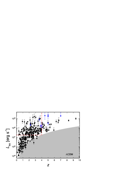
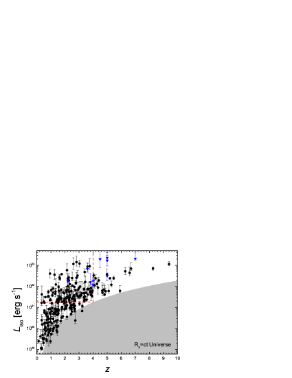
Figure 2: The luminosity-redshift distribution of 254 Swift GRBs in $\Lambda$CDM (left panel) and $R_{\rm h}=ct$ (right panel). The blue dots represent the bursts with redshift upper limits. The shaded regions represent the luminosity threshold adopted in our calculations (see text and equation 18).

Our final sample includes 254 GRBs, whose luminosity-redshift distribution is shown in Figure 2. A determination of $E_{\rm iso}$ requires the assumption of a particular cosmological model. In this figure, we show the resulting distributions for both $\Lambda$CDM (left panel) and $R_{\rm h}=ct$ (right panel). As presented in the various sources used to compile our catalog, quantities such as $E_{\rm iso}$ are estimated assuming a $\Lambda$CDM cosmology. Here, we must therefore recalibrate them for use in $R_{\rm h}=ct$. The differences between these two models are summarized in Melia (2012a,2013a,2013b), Melia & Shevchuk (2012), Melia & Maier (2013), and Wei et al. (2013). The luminosity distance in $\Lambda$CDM is given by the expression

$$D_{L}^{\Lambda{\rm CDM}}(z)={c\over H_{0}}{(1+z)\over\sqrt{\mid\Omega_{k}\mid}}\;sinn\left\{\mid\Omega_{k}\mid^{1/2}\times\int_{0}^{z}{dz\over\sqrt{(1+z)^{2}(1+\Omega_{m}z)-z(2+z)\Omega_{\Lambda}}}\right\}\;,$$ (2)

where $c$ is the speed of light, and $H_{0}$ is the Hubble constant at the present time. In this equation, $\Omega_{m}\equiv\rho_{m}/\rho_{c}$ is the energy density of matter written in terms of today’s critical density, $\rho_{c}\equiv 3c^{2}H_{0}^{2}/8\pi G$. Also, $\Omega_{\Lambda}$ is the similarly defined density of dark energy, and $\Omega_{k}$ represents the spatial curvature of the Universe—appearing as a term proportional to the spatial curvature constant $k$ in the Friedmann equation. In addition, $sinn$ is $\sinh$ when $\Omega_{k}>0$ and $\sin$ when $\Omega_{k}<0$. For a flat Universe with $\Omega_{k}=0$, this equation simplifies to the form $(1+z)c/H_{0}$ times the integral.

In the $R_{\rm h}=ct$ Universe, the luminosity distance is given by the much simpler expression

$$D_{L}^{R_{\rm h}=ct}=\frac{c}{H_{0}}(1+z)\ln(1+z)\;.$$ (3)

The factor $c/H_{0}$ is in fact the gravitational horizon $R_{\rm h}(t_{0})$ at the present time, so we may also write the luminosity distance as

$$D_{L}^{R_{\rm h}=ct}=R_{\rm h}(t_{0})(1+z)\ln(1+z)\;.$$ (4)

We have found the equivalent isotropic energy in the $R_{\rm h}=ct$ Universe using the expression

$${E}_{\rm iso}^{R_{\rm h}=ct}=E_{\rm iso}^{\Lambda{\rm CDM}}\times\left({D^{R_{\rm h}=ct}_{L}\over D^{\Lambda{\rm CDM}}_{L}}\right)^{2}\;,$$ (5)

where $E_{\rm iso}^{\Lambda{\rm CDM}}$ is the previously published value.

3 The Model

The observed rate of GRBs per unit time at redshifts $\in(z,z+dz)$ with luminosity $\in(L,L+dL)$ is given by

$$\frac{dN}{dt\,dz\,dL}=\frac{\dot{\rho}_{\rm GRB}(z)}{1+z}\frac{\Delta\Omega}{4\pi}\frac{dV_{\rm com}(z)}{dz}\,\Phi(L)\;,$$ (6)

where $\dot{\rho}_{\rm GRB}(z)$ is the co-moving rate density of GRBs, $\Phi(L)$ is the beaming-convolved luminosity function (LF), the factor $(1+z)^{-1}$ accounts for the cosmological time dilation and $\Delta\Omega=1.4$ sr is the solid angle covered on the sky by Swift (Salvaterra & Chincarini 2007). The co-moving volume is calculated using

$$\frac{dV_{\rm com}}{dz}=4\pi D_{\rm com}^{2}\frac{dD_{\rm com}}{dz}.$$ (7)

In the standard ($\Lambda$CDM) model, the co-moving luminosity distance is given as

$$D_{\rm com}^{\rm\Lambda CDM}(z)\equiv\frac{c}{H_{0}}\int_{0}^{z}\frac{dz^{\prime}}{\sqrt{\Omega_{\rm m}(1+z^{\prime})^{3}+\Omega_{\Lambda}}}\;,$$ (8)

where we now adopt concordance values of the cosmological parameters: $H_{0}=70$ km $\rm s^{-1}$ $\rm Mpc^{-1}$, $\Omega_{\rm m}=0.3$, and $\Omega_{\Lambda}=0.7$, and assume a spatially flat expansion. In the $R_{\rm h}=ct$ Universe, the co-moving luminosity distance is given by the much simpler expression

$$D_{\rm com}^{R_{\rm h}=ct}(z)=\frac{c}{H_{0}}\ln(1+z)$$ (9)

which, as we have noted previously, has only one free parameter—the Hubble constant $H_{0}$. For the sake of consistency, we will adopt the standard $H_{0}=70$ km $\rm s^{-1}$ $\rm Mpc^{-1}$ throughout this analysis.

As discussed above, we assume that the GRB rate density is related to the cosmic SFR density $R_{\rm SF}(z)$ and a possible evolution effect $f(z)$, given as

$$\dot{\rho}_{\rm GRB}(z)=k_{\rm GRB}R_{\rm SF}(z)f(z)\;,$$ (10)

where $k_{\rm GRB}$ is the GRB formation efficiency to be determined from the observations.

Because of the faintness of sub-luminous galaxies at high redshifts, as well as the uncertainty of the dust extinction (in terms of the amount of dust as well as the dust attenuation law), it is difficult to observe LBG’s at high redshifts. Consequently, the LBG samples are incomplete, and the star formation history at $z\ga 4$ is not well constrained by the data. For relatively low redshifts ($z\la 4$), the star formation rate density $R_{\rm SF}$ has been fitted with a piecewise power law (Hopkins & Beacom 2006; Li 2008), which in $\Lambda$CDM (with the concordance, WMAP parameters) may be written

$$\log_{10}R_{\rm SF}^{\rm\Lambda CDM}(z)=a+b\log_{10}(1+z)\;,$$ (11)

where

$$(a,b)=\left\{\begin{array}[]{ll}(-1.70,3.30),~{}~{}~{}~{}~{}~{}~{}~{}~{}~{}~{}z<0.993\\ (-0.727,0.0549),~{}~{}~{}~{}~{}0.993<z<3.8,\\ \end{array}\right.$$ (12)

and $R_{\rm SF}$ is in units of $\rm M_{\bigodot}$ $\rm yr^{-1}$ $\rm Mpc^{-3}$. To convert from one cosmology to another, our procedure is as follows: the co-moving volume is proportional to the co-moving distance cubed, $V_{\rm com}\propto D_{\rm com}^{3}$, and the co-moving volume between redshifts $z-\Delta z$ and $z+\Delta z$ is $V_{\rm com}(z,\Delta z)\propto D_{\rm com}^{3}(z+\Delta z)-D_{\rm com}^{3}(z-\Delta z)$. Since the luminosity is proportional to the co-moving distance squared, $L\propto D_{\rm com}^{2}$, the SFR density for a given redshift range is (Hopkins 2004)

$$R_{\rm SF}(z)\propto\frac{L(z)}{V_{\rm com}(z,\Delta z)}\propto\frac{D_{\rm com}^{2}(z)}{D_{\rm com}^{3}(z+\Delta z)-D_{\rm com}^{3}(z-\Delta z)}.$$ (13)

Thus, the SFR in the redshift range $z=0-3.8$ for the $R_{\rm h}=ct$ Universe becomes

$$\log R_{\rm SF}^{R_{\rm h}=ct}(z)=a+b\log(1+z)\;,$$ (14)

where

$$(a,b)=\left\{\begin{array}[]{ll}(-1.70,3.52),~{}~{}~{}~{}~{}~{}~{}~{}~{}~{}~{}z<0.993\\ (-0.507,-0.46),~{}~{}~{}~{}~{}0.993<z<3.8.\\ \end{array}\right.$$ (15)

For the GRB luminosity function (LF) $\Phi(L)$, several models have been adopted in the literature: a single power law with an exponential cut-off at low luminosity (exponential LF), a broken power law, and a Schechter function. Here, we use the exponential LF

$$\Phi(L)\propto\left(\frac{L}{L_{\star}}\right)^{-a_{\rm L}}\exp\left(-\frac{L_{\star}}{L}\right)\;,$$ (16)

where $a_{\rm L}$ is the power-law index and $L_{\star}$ is the cutoff luminosity. The normalization constant of the LF is calculated assuming a minimum luminosity $L_{\rm min}=10^{49}$ erg s^-1. The LF will be taken to be non-evolving in this paper.

Finally, when considering an instrument having a flux threshold, the expected number of GRBs with luminosity $L_{\rm iso}>L_{\rm lim}$ and redshift $z\in(z_{1},z_{2})$ during an observational period T should be

$$\begin{split}N=\frac{\Delta\Omega\;T}{4\pi}\int_{z_{1}}^{z_{2}}\frac{\dot{\rho}_{\rm GRB}(z)}{1+z}\frac{dV_{\rm com}(z)}{dz}\;dz\int_{\rm max[L_{\rm min},L_{\rm lim}(z)]}^{\infty}\Phi(L)\;dL\;.\end{split}$$ (17)

The luminosity threshold appearing in equation (17) may be approximated using a bolometric energy flux limit $F_{\rm lim}=1.2\times 10^{-8}$ erg $\rm cm^{-2}$ $\rm s^{-1}$ (Li 2008), for which

$$L_{\rm lim}=4\pi D_{\rm L}^{2}F_{\rm lim}\;,$$ (18)

where $D_{\rm L}$ is the luminosity distance to the burst (either $D_{\rm L}^{\Lambda{\rm CDM}}$ or $D_{\rm L}^{R_{\rm h}=ct}$, as the case may be).

4 A Comparative Analysis of $\Lambda$CDM and The $R_{\rm h}=ct$ Universe

4.1 A possible evolutionary effect

The Swift/BAT trigger is quite complex. Its algorithm has two modes: the count rate trigger and the image trigger (Fenimore et al. 2003; Sakamoto et al. 2008, 2011). Rate triggers are measured on different timescales (4 ms to 64 s), with a single or several backgrounds. Image triggers are found by summing images over various timescales and searching for uncataloged sources. So the sensitivity of the BAT is very difficult to parametrize exactly (Band 2006). Moreover, although the rate density $R_{\rm SF}(z)$ is now reasonably well measured from $z=0$ to $4$, it is not well constrained at $z\ga 4$. To avoid the complications that would arise from the use of a detailed treatment of the Swift threshold and the star formation rate at high-z, we will adopt a model-independent approach by selecting only GRBs with $L_{\rm iso}\geq L_{\rm lim}$ and $z<4$, as Kistler et al. (2008) did in their treatment. The cut in luminosity is chosen to be equal to the threshold at the highest redshift of the sample, i.e., $L_{\rm lim}\approx 1.8\times 10^{51}$ erg $\rm s^{-1}$. The cuts in luminosity and redshift minimize selection effects in the GRB data. With these conditions, our final tally of GRBs is 118 for $\Lambda$CDM and 111 in $R_{\rm h}=ct$. These data are delimited by the red dashed lines in Figure 2.

Now, since $L_{\rm lim}$ is constant, the integral of the LF in equation (17) can be treated as a constant coefficient, no matter what the specific form of $\Phi(L)$ happens to be. That is, we may write

$$\begin{split}N(<z)\propto\int_{0}^{z}R_{\rm SF}(z)\frac{f(z)}{1+z}\frac{dV_{\rm com}}{dz}\;dz\;.\end{split}$$ (19)

Figure 3 shows the cumulative redshift distribution of observed GRBs (steps), normalized over the redshift range $0<z<4$. The gray-shaded region shows how the distribution shifts in the limiting cases of all dark GRBs occurring at $z=0$ or the upper redshift limits determined by Perley et al. (2009), Greiner et al. (2011), and Kr$\ddot{\rm u}$hler et al. (2011). In the left panel of this figure, we assume the $\Lambda$CDM cosmology, and compare the observed GRB cumulative redshift distribution with three types of redshift evolution, characterized through the function $f(z)$. If this function is constant (dotted red line), the expectation from the SFR alone (i.e., the non-evolution case) is incompatible with the observations. If we parameterize the possible evolution effect as $f(z)\propto(1+z)^{\delta}$, we find that the $\chi^{2}$ statistic is minimized for $\delta=0.8$, which is consistent with that of Robertson & Ellis (2012) and Wang (2013). The weak redshift evolution ($\delta=0.8$) can reproduce the observed cumulative GRB rate density best (dashed green line). At the $2\sigma$ confidence level, the value of $\delta$ lies in the range $0.07<\delta<1.53$. In the limiting case where all the dark GRBs are local, the power-law index is constrained to be $-0.56<\delta<0.98$ at the $2\sigma$ confidence level. The peak probability occurs for $\delta=0.21$. Instead, if all the dark GRBs are at their maximum possible redshift, the power-law index moves to $0.19<\delta<1.67$ ($2\sigma$) with a peak near $\delta\approx 0.93$. Clearly, the additional uncertainty arising from the inclusion of dark GRBs is an important consideration. If dark GRBs occur at their maximum allowed redshifts, the distribution is more heavily weighted towards higher values of $z$ and would therefore indicate a stronger redshift dependence of the relationship between the GRB rate and the SFR. We will discuss the third type of evolution shortly.

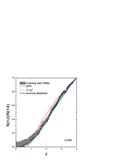
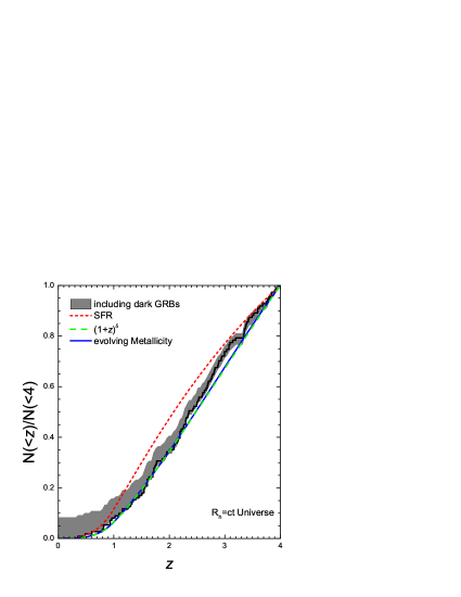
Figure 3: Left: Cumulative distribution of 118 Swift GRBs with $z<4$ and $L_{\rm iso}>1.8\times 10^{51}$ erg $s^{-1}$, assuming the standard ($\Lambda$CDM) model. The black steps and the gray area indicate the cumulative distribution of GRBs with firm reshifts and the uncertainty owing to dark GRBs. Three fitting results using equation (19) are also shown: the red dotted line corresponds to the SFR on its own (i.e., $f(z)$ is constant), the pink dashed line corresponds to $f(z)\propto(1+z)^{\delta}$, with $\delta=0.80$, and the blue solid line corresponds to $f(z)\propto\Theta(\epsilon,z)$, with $\epsilon=0.52$. Right: Same as the left panel, but for 111 Swift GRBs and with $\delta=1.03$ and $\epsilon=0.44$ in the $R_{h}=ct$ Universe.

The collapsar model predicts that long bursts should occur preferentially in metal poor environments. From a theoretical standpoint, this is not surprising since lower metallicity leads to weaker stellar winds and hence less angular momentum loss, resulting in the retention of rapidly rotating cores in stars at the time of their explosion, as implied by simulations of the collapsar model for GRBs (e.g., Woosley 1993b; MacFayden & Woosley 1999; Yoon & Langer 2005). It has therefore been suggested that the observationally required evolution may be due mainly to the cosmic evolution in metallicity.

According to Langer & Norman (2006), the fractional mass density belonging to metallicity below $Z=\epsilon Z_{\odot}$ (where $Z_{\odot}$ is the solar metal abundance, and $\epsilon$ is determined by the metallicity threshold for the production of GRBs) at a given redshift z can be calculated using $\Theta(\epsilon,z)=\hat{\Gamma}(\kappa+2,\epsilon^{\beta}10^{0.15\beta z})/\Gamma(\kappa+2)$, where $\kappa=-1.16$ is the power-law index in the Schechter distribution function of galaxy stellar masses (Panter et al. 2004), $\beta=2$ is the slope of the linear bisector fit to the galaxy stellar mass-metallicity relation (Savaglio 2006), and $\hat{\Gamma}(a,x)$ and $\Gamma(x)$ are the incomplete and complete Gamma functions, respectively. To test this interpretation of the anomalous evolution, we parameterize the evolution function as $f(z)\propto\Theta(\epsilon,z)$, and show the result of an evolving metallicity as a blue line in the left panel of Figure 3. This theoretical curve agrees very well with the observations. The best fit to the observations yields $\epsilon=0.52$. At the $2\sigma$ confidence level, the value of $\epsilon$ lies in the range $0.19<\epsilon<0.85$. A comparison between this curve and that obtained with $f(z)=(1+z)^{0.8}$ shows that the differences between these two fits is not very significant. Therefore, we confirm that the anomalous evolution in $\Lambda$CDM may be due to an evolving metallicity. However, in contrast to previous studies that suggest a metallicity cut of $Z_{\rm th}\la 0.3Z_{\odot}$ (Woosley & Heger 2006; Langer & Norman 2006; Salvaterra & Chincarini 2007; Li 2008; Campisi et al. 2010; Salvaterra et al. 2012), we find that only the higher metallicity cut $Z_{\rm th}=0.52Z_{\odot}$ is consistent with the data, in agreement with the conclusions of Hao & Yuan (2013). It is worth mentioning that the higher metallicity cut is also more consistent with recent studies of the long GRB host galaxies (Graham et al. 2009; Levesque et al. 2010a,b; Michalowski et al. 2012).

The right panel of Figure 3 shows the cumulative redshift distribution of 111 Swift GRBs with $L_{\rm lim}=1.8\times 10^{51}$ erg $\rm s^{-1}$ and $z<4$ in the $R_{\rm h}=ct$ Universe. The result of our fitting from the SFR alone (i.e., with a constant $f[z]$) is shown as a dotted red line, which again is incompatible with the observations. An additional evolutionary effect, parametrized as $f(z)\propto(1+z)^{1.03}$ is required (dashed green line). At the $2\sigma$ confidence level, the value of $\delta$ lies in the range $0.32<\delta<1.71$. If the dark GRB sample with redshift limits is assumed to be local ($z\approx 0$), the $2\sigma$ interval is $-0.38<\delta<1.12$ with a peak near $\delta=0.37$. Instead, if all dark GRBs are at their maximum possible redshift, the power-law index moves to $0.43<\delta<1.87$ ($2\sigma$) with a peak near $\delta\approx 1.15$. Clearly, if dark GRBs occur at their maximum allowed redshifts, the distribution is more heavily weighted toward higher redshifts and the extra redshift evolution effect still exists in the $R_{\rm h}=ct$ Universe. If we instead designate the evolutionary effect as $f(z)\propto\Theta(\epsilon,z)$, the evolving metallicity agrees very well with the observations (blue line). The best fit to the observations yields $\epsilon=0.44\pm 0.28(2\sigma)$. Clearly, the evolutionary effect in both the $\Lambda$CDM and the $R_{\rm h}=ct$ cosmologies can be accounted for with a metallicity cutoff at $Z_{\rm th}$ ($0.52Z_{\odot}$ for the former and $0.44Z_{\odot}$ for the latter).

In the next section, we will consider the implications of these findings for the star-formation history, assuming that GRBs trace both star formation and a possible evolutionary effect. We will adopt the best fitting values $\delta=0.80$ or $\epsilon=0.52$ for a reasonable description of the evolutionary effect in $\Lambda$CDM, and $\delta=1.03$ or $\epsilon=0.44$ in the $R_{\rm h}=ct$ Universe.

4.2 Constraints on the high-z star formation history in $\Lambda$CDM and the $R_{\rm h}=ct$ Universe

The SFR is well measured at low-z now. For high-z ($z\ga 4$), a decrease to the SFR was seemingly implied by the work of Hopkins & Beacom (2006), which was confirmed by observations of LBGs and GRBs. Nonetheless, given the poor coverage of these remote regions, the SFR trends towards high-z are still rather ambiguous. For this reason, previous studies have included all possibilities: one in which the star-formation history continues to plateau, or in which it drops off, or even increases with increasing redshift (see, e.g., Daigne et al. 2006). In our analysis, we will introduce a free parameter $\alpha$ to parameterize the high-z history as a power law at redshifts $z\geq 3.8$:

$$R_{\rm SF}(z)=\left\{\begin{array}[]{ll}0.20\left(\frac{1+z}{4.8}\right)^{\alpha},~{}~{}~{}~{}~{}{\rm for~{}~{}~{}\Lambda CDM}\\ 0.15\left(\frac{1+z}{4.8}\right)^{\alpha},~{}~{}~{}~{}~{}{\rm for~{}~{}~{}R_{\rm h}=ct},\\ \end{array}\right.$$ (20)

and we will attempt to constrain this index $\alpha$ using the GRB observations. The normalization constant in this expression is set by the requirement that $R_{\rm SF}$ be continuous across $z=3.8$.

We optimize the values of each model’s free parameters, including the index $\alpha$ of high-z SFR, the GRB formation efficiency $k_{\rm GRB}$, and the GRB LF, by minimizing the $\chi^{2}$ statistic jointly fitting the observed redshift distribution and luminosity distribution of bursts in our sample with firm measurements of their redshift. The observed number of GRBs in each redshift bin $z\in(z_{1},z_{2})$ is given by equation (17), while, the observed number of events in each luminosity bin $L_{\rm iso}\in(L_{\rm 1},L_{\rm 2})$ is given by

$$\begin{split}N_{(L_{1},L_{2})}=\frac{\Delta\Omega\;T}{4\pi}\int_{L_{1}}^{L_{2}}\Phi(L)\;dL\int_{0}^{z_{\rm max}(L)}\frac{\dot{\rho}_{\rm GRB}(z)}{1+z}\frac{dV_{\rm com}(z)}{dz}\,dz\;,\end{split}$$ (21)

where $T\sim 8.6$ yr is the observational period, and $z_{\rm max}(L_{\rm iso})$ is the maximum redshift out to which a GRB of luminosity $L_{\rm iso}$ can be detected; this is obtained by solving the equation $L_{\rm lim}(z)=L_{\rm iso}$ for each assumed cosmology.

Table 2: Best-fitting Results in Different Cosmological Models.

Model	$\alpha$	$k_{\rm GRB}$	$L_{\star}$	$a_{L}$	$\chi^{2}$	AIC
		($10^{-9}$ $M_{\odot}^{-1}$)	($10^{49}$ erg $\rm s^{-1}$)
		$\Lambda$CDM
No evol	$-2.48_{-1.46}^{+1.45}$	$6.21_{-0.88}^{+0.36}$	$1.03_{-0.39}^{+0.39}$	$1.41_{-0.04}^{+0.03}$	66.5	74.5
Density evol ($\delta=0.80$)	$-3.06_{-2.01}^{+2.01}$	$4.39_{-1.12}^{+0.67}$	$0.46_{-0.48}^{+0.48}$	$1.51_{-0.07}^{+0.08}$	55.4	63.4
Metallicity evol ($\epsilon=0.52$)	$-2.41_{-2.09}^{+1.87}$	$13.3_{-2.6}^{+3.1}$	$1.19_{-0.29}^{+0.29}$	$1.51_{-0.05}^{+0.09}$	56.0	64.0
		$R_{\rm h}=ct$
No evol	$-3.27_{-1.39}^{+1.44}$	$7.22_{-1.05}^{+0.33}$	$1.11_{-0.68}^{+0.68}$	$1.40_{-0.04}^{+0.03}$	67.4	75.4
Density evol ($\delta=1.03$)	$-4.47_{-2.34}^{+2.30}$	$3.77_{-1.01}^{+0.49}$	$1.06_{-0.66}^{+0.66}$	$1.54_{-0.05}^{+0.11}$	58.6	66.6
Metallicity evol ($\epsilon=0.44$)	$-3.60_{-2.45}^{+2.45}$	$19.5_{-4.4}^{+4.2}$	$1.11_{-0.26}^{+0.34}$	$1.50_{-0.02}^{+0.14}$	54.3	62.3

^Notes.The total number of data points in the fit is 42, including 33 points for the redshift distribution and 9 points for the luminosity distribution.

We report the best-fit parameters together with their $1\sigma$ confidence level for different models in Table 2. In the last two columns, we give the total $\chi^{2}$ value (i.e., the sum of the $\chi^{2}$ values obtained from the fit of the redshift and luminosity distributions) and the Akaike information criterion (AIC) score, respectively. For each fitted model, the AIC is given by ${\rm AIC}=\chi^{2}+2k$, where $k$ is the number of free parameters. If there are three models for the data, $\mathcal{M}_{1}$, $\mathcal{M}_{2}$, and $\mathcal{M}_{3}$, and they have been separately fitted, the one with the least resulting AIC is the one favored by this criterion. A more quantitative ranking of models can be computed as follows. If ${\rm AIC}_{\alpha}$ comes from model $\mathcal{M}_{\alpha}$, the unnormalized confidence in $\mathcal{M}_{\alpha}$ is given by the “Akaike weight” $\exp(-{\rm AIC}_{\alpha}/2)$. Informally, in a three-way comparison, the relative probability that $\mathcal{M}_{\alpha}$ is statistically preferred is

$${\cal L}(\mathcal{M}_{\alpha})=\frac{\exp(-{\rm AIC}_{\alpha}/2)}{\exp(-{\rm AIC}_{1}/2)+\exp(-{\rm AIC}_{2}/2)+\exp(-{\rm AIC}_{3}/2)}\;.$$ (22)

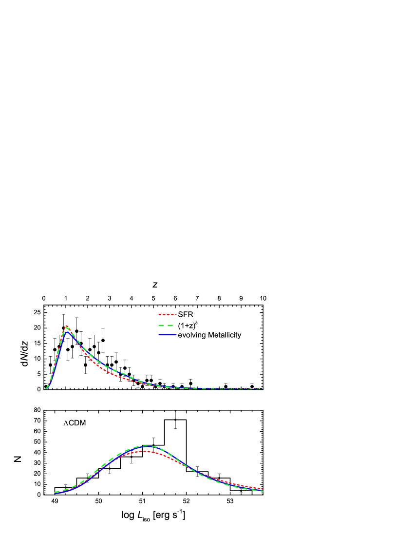
Figure 4: Distributions in $z$ and $L$ of 244 Swift GRBs with firm redshift measurements in the $\Lambda$CDM cosmology (the solid points and steps, with the number of GRBs in each bin indicated by a dark point with Poisson error bars). The dotted lines (red) show the expected distribution for the case of no evolution. The results of density and metallicity evolution models are shown with green dashed lines and blue solid lines, respectively.

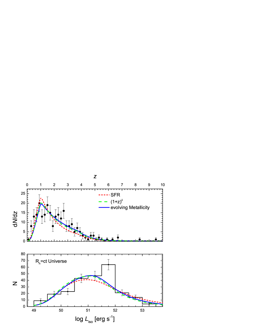
Figure 5: Same as Figure 4, but for the $R_{\rm h}=ct$ Universe.

4.2.1 No-Evolution Model

This model is for the GRB rate that purely follows the SFR. Figure 4 shows the $z$ and $L$ distributions of 244 Swift GRBS in the $\Lambda$CDM cosmology. If the function $f(z)$ is constant (dotted red line), the expectation from the SFR alone (i.e., the non-evolution case) does not provide a good representation of the observed $z$ and $L$ distributions of our sample. In particular, the rate of GRBs at high-z is under-predicted and the fit of the $L$ distribution is not as good as those of the density evolution model or metallicity threshold model, more fully described below. This is confirmed by a more detailed statistical analysis. Indeed, on the basis of the AIC model selection criterion, we can discard this model as having a likelihood of only $\sim 0.2\;\%$ of being correct compared to the other two $\Lambda$CDM models.

Figure 5 shows the redshift and luminosity distributions of 244 Swift GRBS in the $R_{\rm h}=ct$ Universe. The results of our fitting from the SFR alone (i.e., with a constant $f[z]$) are indicated with dotted red lines, which again are incompatible with the observations. On the basis of the AIC model selection criterion, we can discard the no-evolution model as having a likelihood of only $\sim 0.1\;\%$ of being correct compared to the other two $R_{\rm h}=ct$ models.

4.2.2 Density Evolution Model

This model assumes that the GRB rate follows the SFR in conjunction with an additional evolution characterized by $(1+z)^{\delta}$. In $\Lambda$CDM, we find that $\delta=0.80$ reproduces the observed $z$ and $L$ distributions (green dashed lines in Figure 4) quite well. In this model, the slope of the high-z SFR is characterized by an index $\alpha=-3.06_{-2.01}^{+2.01}$. The range of high-z SFH’s with $\alpha\in(-5.07,-1.05)$ is marked with a shaded band in figure 1, in comparison with the available data. It is interesting to note that Wang (2013) derived a similar slope ($\alpha=-3.0$) for the high-z SFR. Wu et al. (2012) showed that the GRB formation rate in $\Lambda$CDM decreases with a power index of $\sim-3.8$ for $z\ga 4$, in good agreement with the SFR we derive here at the $1\sigma$ confidence level. Using the AIC model selection criterion, we find that among the $\Lambda$CDM models, this one is statistically preferred with a relative probability $\sim 57.3\;\%$.

In the $R_{\rm h}=ct$ Universe, we simultaneously fit the observed $z$ and $L$ distributions of Swift GRBs using $\dot{\rho}_{\rm GRB}(z)=k_{\rm GRB}R_{\rm SFR}(z)(1+z)^{\delta}$, together with the piecewise smooth $R_{\rm SFR}(z)$ concatenated from equations (14) and (20); the best fit corresponds to $\delta=1.03$. We find that a high-z SFR with slope $\alpha=-4.47_{-2.34}^{+2.30}$ is required to reproduce both the observed $z$ and $L$ distributions (green dashed lines in figure 5). Again using the AIC model selection criterion, we find that this model is somewhat disfavored statistically compared to the other two $R_{\rm h}=ct$ models, with a relative probability of $\sim 10.4\;\%$.

4.2.3 Metallicity Evolution Model

This model assumes that the GRB rate is proportional to the star formation history with an additional evolution in cosmic metallicity (i.e., $f[z]\propto\Theta[\epsilon,z]$). For $\Lambda$CDM, we find that a high-$z$ SFR with index $\alpha=-2.41_{-2.09}^{+1.87}$ and a metallicity evolution parameter $\epsilon=0.52$ fits the data best (blue solid lines in Figure 4). The $\chi_{\rm dof}^{2}$ for this fit is $56.0/42=1.33$. In general, fitting the observations with this model produces better consistency than the non-evolution model. According to the AIC, the metallicity evolution model in $\Lambda$CDM is slightly disfavored compared to the more general density evolution model, but the differences are statistically insignificant ($\sim 42.5\;\%$ for the former versus $\sim 57.3\;\%$ for the latter). We conclude that in the context of $\Lambda$CDM, the required density evolution may be due to an evolving metallicity.

In the context of the $R_{\rm h}=ct$ Universe, the best fit is produced with a high-$z$ SFR with index $\alpha=-3.60_{-2.45}^{+2.45}$ and a metallicity evolution with $\epsilon=0.44$. The $\chi_{\rm dof}^{2}$ for this fit is $54.3/42=1.29$. This model is represented by the blue solid lines in figure 5. The AIC shows that the likelihood of this model being correct is $\sim 89.5\;\%$ compared to the other two $R_{\rm h}=ct$ models examined above. Unlike the situation with $\Lambda$CDM, here there is a clear indication that abundance evolution is required to account for the SFR/GRB data.

5 Discussion and Conclusions

We have used the cumulative redshift distribution of the latest sample of Swift GRBs above a fixed luminosity limit, together with the star formation history over the interval $z\in(0,4)$, to compare the predictions of $\Lambda$CDM and the $R{\rm h}=ct$ Universe. With $\Lambda$CDM as the background spacetime, earlier work had already demonstrated that in this cosmology the SFR underproduces the GRB rate density at high redshifts. It has been suggested that this effect can be understood if a modest evolution, parameterized as $f(z)=(1+z)^{0.80}$, is included; we have confirmed in both $\Lambda$CDM and $R_{\rm h}=ct$ that this factor may be readily explained as an evolution in metallicity. However, we have also found that a comparison with the observational data shows that a relatively high metallicity cut ($Z=0.52Z_{\odot}$ in $\Lambda$CDM and $Z=0.44Z_{\odot}$ in $R_{\rm h}=ct$) is required, in contrast to previous work that suggested LGRBs occur preferentially in low metallicity environments, i.e., $Z\sim 0.1-0.3Z_{\odot}$.

For both cosmologies, we have shown that if these results are correct, then by assuming that such trends continue beyond $z\simeq 4$, the adoption of a simple power-law approximation for the high-z ($\ga 3.8$) SFR , i.e., $R_{\rm SF}\propto[(1+z)/4.8]^{\alpha}$, we may also constrain the slope $\alpha$ using the GRB data. We have found for $\Lambda$CDM that the SFR at $z\ga 3.8$ shows a decay with slope $\alpha=-2.41_{-2.09}^{+1.87}$. And using a simple relationship between the GRB rate density and the SFR, including an evolution in metallicity, we have demonstrated that the $z$ and $L$ distributions of 244 Swift GRBs can be well fitted by our updated SFH, using a threshold in the metallicity for GRB production.

The best fit for the redshift distribution of the Swift GRBs in the $R_{\rm h}=ct$ Universe requires a slightly different rate than that in $\Lambda$CDM, though still with an additional evolutionary effect, which could be a high metallicity cut of $Z=0.44Z_{\odot}$. Assuming that the GRB rate is related to the SFR with this evolving metallicity, we have found that in the $R_{\rm h}=ct$ Universe the slope of the high-z SFR would be $\alpha=-3.60_{-2.45}^{+2.45}$.

The principal goal of this work has been to directly compare the predictions of $\Lambda$CDM and $R_{\rm h}=ct$ and their ability to account for the GRB/SFR observations. Aside from the issue of whether or not the GRB-redshift distribution is consistent with the SFR in either model, we have also examined which of these two cosmologies fits the data better, and is therefore statistically preferred by the Aikake Information Criterion in a one-on-one comparison.

To keep the complexity of this problem manageable, we have chosen to find the best fits to the data by optimizing four free parameters ($\alpha$, $k_{\rm GRB}$, $L_{\star}$ and $a_{L}$), though the models themselves were held fixed by the concordance values of $H_{0}$, $\Omega_{m}$, $\Omega_{\Lambda}$ and the dark-energy equation-of-state in the case of $\Lambda$CDM, and the same value of $H_{0}$ for $R_{\rm h}=ct$. The two models produce very similar profiles in the distance-redshift relationship (Melia 2012a; Wei et al. 2013), so it is not very surprising to see that both can account quite well for the observed SFR-GRB rate correlation.

However, the AIC does not favor these models equally. From Table 2, we find that a direct comparison between the best $\Lambda$CDM fit (entry 2 in this table) and the best $R_{\rm h}=ct$ fit (entry 6) favors the latter with a relative probability $\sim 63.4\;\%$ versus $\sim 36.6\;\%$ for the standard model. If we further assume that the required evolutionary effect is indeed due to changes in metallicity, so that we now compare entries 3 and 6 in Table 2, then the AIC favors $R_{\rm h}=ct$ with a relative probability $\sim 70.0\;\%$ versus $\sim 30.0\;\%$ for $\Lambda$CDM. However, if the required evolutinary effect is simply due to density and not changes in metallicity (entries 2 and 5), the AIC favors $\Lambda$CDM with a relative probability of $\sim 83.2\;\%$ versus $\sim 16.8\;\%$ for $R_{\rm h}=ct$.

The statistical significance of these likelihoods has been investigated theoretically, e.g., by Yanagihara & Ohmoto (2005). Its variability has also been studied empirically; for example, by repeatedly comparing $\Lambda$CDM to other cosmological models on the basis of data sets generated by a bootstrap method (Tan & Biswas 2012). It is known that the AIC is increasingly accurate when the number of data points is large, but it is felt that in all cases, the magnitude of the difference $\Delta=\allowbreak{\rm AIC}_{2}-\nobreak{\rm AIC}_{1}$ should provide a numerical assessment of the evidence that model 1 is to be preferred over model 2. A rule of thumb that has been used in the literature is that if $\Delta\la 3$, it is mildly strong; and if $\Delta\ga 5$, it is quite strong.

Therefore, our conclusion from the comparative study we have reported here is that—based on the currently available GRB/SFR observations—the $R_{\rm h}=ct$ Universe is mildly favored over $\Lambda$CDM in a one-on-one comparison if the required evolution is due to changes in metallicity (for which $\Delta\approx 1.7$). However, $\Lambda$CDM is mildly favored over $R_{\rm h}=ct$ (with $\Delta\approx 3.2$) if instead the evolution is with density.

The prevailing view at the moment seems to be that changes in metallicity are responsible for the required evolution so, in this context, the GRB/SFR data tend to be more consistent with the predictions of $R_{\rm h}=ct$ than those of the concordance model. Note that the likelihood estimates we have made here were based on the use of priors for $\Lambda$CDM. Were we to optimize $H_{0}$ along with the other four parameters (for both models), and $\Omega_{m}$, $\Omega_{\Lambda}$ and the dark-energy equation of state for $\Lambda$CDM, we could certainly lower their $\chi^{2}$ for the best fits, but the AIC strongly penalizes models with many free parameters. The $\chi^{2}$ values listed for $\Lambda$CDM in Table 2 would need to decrease by at least 6 in order to compensate for the increase due to the factor $2k$ in the expression ${\rm AIC}=\chi^{2}+2k$. This seems unlikely since the fits using the concordance model are already rather good.

Refinements in future measurements of the GRB rate and SFR may show that the currently believed explanation for their differences (i.e., an evolution in metallicity) is incorrect. In that case, a reassessment of these comparisons may produce different results. As of now, however, it appears that the SFR underproduces the observed GRB rate unless some additional evolution were present to broaden their disparity with increasing redshift. We have found that such an evolution is consistent with a relatively high metallicity cutoff for the LGRBs.

References

- Band (2006) Band D. L., 2006, ApJ, 644, 378
- Blain & Natarajan (2000) Blain A. W., Natarajan P., 2000, MNRAS, 312, L35
- Bouwens et al. (2008) Bouwens R. J., Illingworth G. D., Franx M., Ford H., 2008, ApJ, 686, 230
- Butler, Bloom, & Poznanski (2010) Butler N. R., Bloom J. S., Poznanski D., 2010, ApJ, 711, 495
- Butler et al. (2007) Butler N. R., Kocevski D., Bloom J. S., Curtis J. L., 2007, ApJ, 671, 656
- Campisi, Li, & Jakobsson (2010) Campisi M. A., Li L.-X., Jakobsson P., 2010, MNRAS, 407, 1972
- Cao et al. (2011) Cao X.-F., Yu Y.-W., Cheng K. S., Zheng X.-P., 2011, MNRAS, 416, 2174
- Chapman et al. (2007) Chapman R., Tanvir N. R., Priddey R. S., Levan A. J., 2007, MNRAS, 382, L21
- Chary, Berger, & Cowie (2007) Chary R., Berger E., Cowie L., 2007, ApJ, 671, 272
- Chornock et al. (2010) Chornock R., et al., 2010, arXiv, arXiv:1004.2262
- Cobb et al. (2006) Cobb B. E., Bailyn C. D., van Dokkum P. G., Natarajan P., 2006, ApJ, 645, L113
- Coward et al. (2008) Coward D. M., Guetta D., Burman R. R., Imerito A., 2008, MNRAS, 386, 111
- Coward et al. (2013) Coward D. M., Howell E. J., Branchesi M., Stratta G., Guetta D., Gendre B., Macpherson D., 2013, MNRAS, 432, 2141
- Dado & Dar (2013) Dado S., Dar A., 2013, arXiv, arXiv:1307.5556
- Daigne, Rossi, & Mochkovitch (2006) Daigne F., Rossi E. M., Mochkovitch R., 2006, MNRAS, 372, 1034
- Elliott et al. (2012) Elliott J., Greiner J., Khochfar S., Schady P., Johnson J. L., Rau A., 2012, A&A, 539, A113
- Fenimore et al. (2003) Fenimore E. E., Palmer D., Galassi M., Tavenner T., Barthelmy S., Gehrels N., Parsons A., Tueller J., 2003, AIPC, 662, 491
- Graham et al. (2009) Graham J. F., Fruchter A. S., Kewley L. J., Levesque E. M., Levan A. J., Tanvir N. R., Reichart D. E., Nysewander M., 2009, AIPC, 1133, 269
- Greiner et al. (2011) Greiner J., et al., 2011, A&A, 526, A30
- Guetta & Piran (2007) Guetta D., Piran T., 2007, JCAP, 7, 3
- Hao & Yuan (2013) Hao J.-M., Yuan Y.-F., 2013, ApJ, 772, 42
- Hjorth et al. (2012) Hjorth J., et al., 2012, ApJ, 756, 187
- Hjorth et al. (2003) Hjorth J., et al., 2003, Natur, 423, 847
- Hopkins (2004) Hopkins A. M., 2004, ApJ, 615, 209
- Hopkins & Beacom (2006) Hopkins A. M., Beacom J. F., 2006, ApJ, 651, 142
- Ishida, de Souza, & Ferrara (2011) Ishida E. E. O., de Souza R. S., Ferrara A., 2011, MNRAS, 418, 500
- Kistler et al. (2009) Kistler M. D., Yüksel H., Beacom J. F., Hopkins A. M., Wyithe J. S. B., 2009, ApJ, 705, L104
- Kistler et al. (2008) Kistler M. D., Yüksel H., Beacom J. F., Stanek K. Z., 2008, ApJ, 673, L119
- Kouveliotou et al. (1993) Kouveliotou C., Meegan C. A., Fishman G. J., Bhat N. P., Briggs M. S., Koshut T. M., Paciesas W. S., Pendleton G. N., 1993, ApJ, 413, L101
- Krühler et al. (2011) Krühler T., et al., 2011, A&A, 534, A108
- Lamb & Reichart (2000) Lamb D. Q., Reichart D. E., 2000, ApJ, 536, 1
- Langer & Norman (2006) Langer N., Norman C. A., 2006, ApJ, 638, L63
- Le & Dermer (2007) Le T., Dermer C. D., 2007, ApJ, 661, 394
- Levesque et al. (2010) Levesque E. M., Kewley L. J., Berger E., Zahid H. J., 2010a, AJ, 140, 1557
- Levesque et al. (2010) Levesque E. M., Kewley L. J., Graham J. F., Fruchter A. S., 2010b, ApJ, 712, L26
- Li (2008) Li L.-X., 2008, MNRAS, 388, 1487
- Liang et al. (2007) Liang E., Zhang B., Virgili F., Dai Z. G., 2007, ApJ, 662, 1111
- Lu et al. (2012) Lu R.-J., Wei J.-J., Qin S.-F., Liang E.-W., 2012, ApJ, 745, 168
- MacFadyen & Woosley (1999) MacFadyen A. I., Woosley S. E., 1999, ApJ, 524, 262
- Mannucci et al. (2007) Mannucci F., Buttery H., Maiolino R., Marconi A., Pozzetti L., 2007, A&A, 461, 423
- Melia (2012) Melia F., 2012a, AJ, 144, 110
- Melia (2012) Melia F., 2012b, arXiv, arXiv:1205.2713
- Melia (2013) Melia F., 2013a, ApJ, 764, 72
- Melia (2013) Melia F., 2013b, A&A, 553, 76
- Melia & Shevchuk (2012) Melia F., Shevchuk A. S. H., 2012, MNRAS, 419, 2579
- Melia (2013) Melia F., 2013, ApJ, 764, 72
- Melia & Maier (2013) Melia, F. & Maier, R. S. 2013, MNRAS, 432, 2669
- Michałowski et al. (2012) Michałowski M. J., et al., 2012, ApJ, 755, 85
- Ota et al. (2008) Ota K., et al., 2008, ApJ, 677, 12
- Paczynski (1998) Paczynski B., 1998, ApJ, 494, L45
- Panter, Heavens, & Jimenez (2004) Panter B., Heavens A. F., Jimenez R., 2004, MNRAS, 355, 764
- Perley et al. (2009) Perley D. A., et al., 2009, AJ, 138, 1690
- Perley & Perley (2013) Perley D. A., Perley R. A., 2013, ApJ, 778, 172
- Piran (2004) Piran T., 2004, RvMP, 76, 1143
- Porciani & Madau (2001) Porciani C., Madau P., 2001, ApJ, 548, 522
- Qin et al. (2010) Qin S.-F., Liang E.-W., Lu R.-J., Wei J.-Y., Zhang S.-N., 2010, MNRAS, 406, 558
- Robertson & Ellis (2012) Robertson B. E., Ellis R. S., 2012, ApJ, 744, 95
- Sakamoto et al. (2008) Sakamoto T., et al., 2008, ApJS, 175, 179
- Sakamoto et al. (2011) Sakamoto T., et al., 2011, ApJS, 195, 2
- Salvaterra et al. (2012) Salvaterra R., et al., 2012, ApJ, 749, 68
- Salvaterra & Chincarini (2007) Salvaterra R., Chincarini G., 2007, ApJ, 656, L49
- Salvaterra et al. (2009) Salvaterra R., Guidorzi C., Campana S., Chincarini G., Tagliaferri G., 2009, MNRAS, 396, 299
- Savaglio (2006) Savaglio S., 2006, NJPh, 8, 195
- Shao et al. (2011) Shao L., Dai Z.-G., Fan Y.-Z., Zhang F.-W., Jin Z.-P., Wei D.-M., 2011, ApJ, 738, 19
- Soderberg et al. (2004) Soderberg A. M., et al., 2004, Natur, 430, 648
- Stanek et al. (2003) Stanek K. Z., et al., 2003, ApJ, 591, L17
- Tan & Biswas (2012) Tan, M. Y. J. & Biswas, R. 2012, MNRAS, 419, 3292
- Totani (1997) Totani T., 1997, ApJ, 486, L71
- Verma et al. (2007) Verma A., Lehnert M. D., Förster Schreiber N. M., Bremer M. N., Douglas L., 2007, MNRAS, 377, 1024
- Virgili et al. (2011) Virgili F. J., Zhang B., Nagamine K., Choi J.-H., 2011, MNRAS, 417, 3025
- Wanderman & Piran (2010) Wanderman D., Piran T., 2010, MNRAS, 406, 1944
- Wang (2013) Wang F. Y., 2013, A&A, 556, A90
- Wang & Dai (2011) Wang F. Y., Dai Z. G., 2011, ApJ, 727, L34
- Wang & Dai (2009) Wang F. Y., Dai Z. G., 2009, MNRAS, 400, L10
- Wei, Wu, & Melia (2013) Wei J.-J., Wu X.-F., Melia F., 2013, ApJ, 772, 43
- Wijers et al. (1998) Wijers R. A. M. J., Bloom J. S., Bagla J. S., Natarajan P., 1998, MNRAS, 294, L13
- Woosley (1993) Woosley S. E., 1993a, AAS, 25, 894
- Woosley (1993) Woosley S. E., 1993b, ApJ, 405, 273
- Woosley & Bloom (2006) Woosley S. E., Bloom J. S., 2006, ARA&A, 44, 507
- Woosley & Heger (2006) Woosley S. E., Heger A., 2006, ApJ, 637, 914
- Wu et al. (2012) Wu S.-W., Xu D., Zhang F.-W., Wei D.-M., 2012, MNRAS, 423, 2627
- Xu & Wei (2009) Xu C.-y., Wei D.-m., 2009, ChA&A, 33, 151
- Yanagihara et al. (2005) Yanagihara, H. & Ohmoto, C. 2005, J. Statist. Plann. Inference, 133, 417
- Yüksel & Kistler (2007) Yüksel H., Kistler M. D., 2007, PhRvD, 75, 083004
- Yüksel et al. (2008) Yüksel H., Kistler M. D., Beacom J. F., Hopkins A. M., 2008, ApJ, 683, L5
- Yoon & Langer (2005) Yoon S.-C., Langer N., 2005, A&A, 443, 643
- Zhang (2007) Zhang B., 2007, ChJAA, 7, 1
- Zhang & Mészáros (2004) Zhang B., Mészáros P., 2004, IJMPA, 19, 2385