Results of the Swift Monitoring Campaign of the X-ray Binary 4U 1957+11: Constraints on Binary Parameters

Abstract

We present new results of uniform spectral analysis of Swift/XRT observations of the X-ray binary system 4U 1957+11. This includes 26 observations of the source made between MJD 54282–55890 (2007 July 01 – 2011 November 25). All 26 spectra are predominantly thermal, and can be modeled well with emission from an accretion disk around a black hole. We analyze all 26 spectra jointly using traditional $\chi^{2}$ fitting as well as Markov Chain Monte Carlo simulations. The results from both methods agree, and constrains on model parameters like inclination, column density, and black hole spin. These results indicate that the X-ray emitting inner accretion disk is inclined to our line-of-sight by $77.6^{+1.5}_{-2.2}$ degrees. Additionally, the other constraints we obtain on parameters like the column density and black hole spin are consistent with previous X-ray observations. Distances less than 5 kpc are unlikely and not only ruled out based on our analysis but also from other independent observations. Based on model-derived bolometric luminosities, we require the source distance to be $>$10 kpc if the black hole’s mass is $>$10 M_⊙. If the hole’s mass is $<$10 M_⊙, then the distance could be in the range of 5–10 kpc.

1. Introduction

4U 1957+11 is a bright, persistent X-ray source with soft X-ray (2–12 keV) flux levels between 20–70 milli-Crab since its discovery in 1973 (Giacconi et al., 1974). Yet surprisingly little is known about this binary system. While the lack of X-ray eclipses in this system suggests that the orbital inclination is likely less than 85°, modeling the optical modulation gives only a weak constraint of $\sim 20\arcdeg<i<70\arcdeg$ (Mason et al., 2012). Neither the distance to the system nor the accretor’s mass is well known. However, examining the equivalent width of the Ne ix 13.45Å line created in the ISM, Nowak et al. (2008) and Yao et al. (2008) have suggested a minimum distance of 5 kpc. In the absence of any dynamical mass measurement, analysis of X-ray/optical data from the source at various points of time have suggested that it could either be a neutron star (Yaqoob et al., 1993; Singh et al., 1994; Ricci et al., 1995; Robinson et al., 2012) or a black hole (Wijnands et al., 2002; Nowak et al., 2008, 2012). The morphology of the optical light curve of 4U 1957+11 varies with time. However observations densely sampled in time reveals a modulation with 9.33 hour period, which is usually thought to be the orbital period of this system (Thorstensen, 1987; Bayless et al., 2011; Mason et al., 2012).

The column density (N_H) in the direction of 4U 1957+11 is quite small (1–2$\times$$10^{21}$ atoms cm^-2), providing a clear view of the disk. Furthermore, the high-resolution grating data obtained by Chandra and XMM-Newton, and analyzed by Nowak et al. (2008), show only absorption lines due to the ISM and no lines intrinsic to the source.

Nowak et al. (2008) have analyzed the entire set of Rossi X-ray Timing Explorer (RXTE) observations, as well as Chandra and XMM-Newton observations of this source. More recently Nowak et al. (2012) have also presented their analysis of Suzaku data of this source. The predominantly soft spectrum and very low fractional variability (Nowak & Wilms, 1999; Wijnands et al., 2002; Nowak et al., 2008) are characteristic of 4U 1957+11 being in a canonical soft state. Recent radio non-detection of 4U 1957+11 with an upper limit of of 11.4 $\mu$Jy/beam using the Jansky Very Large Array (JVLA) at 5–7 GHz by Russell et al. (2011) is also consistent with the prevalent wisdom, a.k.a. the jet–disk paradigm, where jet production is strongly quenched in sources that are in a soft state.

Recent works critically examining the X-ray spectral and timing properties using Chandra, XMM-Newton, and RXTE (Nowak et al., 2008, 2012) have suggested that the system harbors a black hole, and that it may be the fastest spinning hole known so far. In this work we assume that the accretor is a BH and test the validity of this assumption under a wide range of plausible parameter space.

We present the details of the Swift observations and data analysis in §2. We then discuss spectral modeling in §3, starting with simple, phenomenological accretion disk plus power law models in §3.1 and then moving towards more physically motivated disk models in §3.2. Joint analysis of all the observations using traditional $\chi^{2}$ fitting technique is presented in §3.3 and that using Markov Chain Monte Carlo (MCMC) simulations is presented in §3.4. Finally, our conclusions are summarized in §4.

2. Swift monitoring campaign of 4U 1957+11

As part of the Swift observatory’s (Gehrels et al., 2004) Guest Observing program number 7100116, 4U 1957+11 was observed 21 times between MJD 55700–55890 (2011 May 19 –2011 November 25). Prior to this monitoring campaign 4U 1957+11 was also observed 5 times with Swift. With an average flux of $\sim 1.5\times 10^{-9}$ erg/s/cm², the source is quite bright in the X-ray telescope’s bandpass (XRT, Burrows et al. 2005). Thereofre these observations were carried out in windowed timing (WT) mode to avoid pileup. The observation logs are presented in Table 1.

The data extraction and reduction were performed using the Heasoft software (v6.12) developed and maintained by NASA’s High Energy Astrophysics Science Archive Research Center (HEASARC). We followed the extraction steps outlined in Reynolds & Miller (2013). The raw data were reprocessed using the xrtpipeline command to ensure that the latest instrument calibrations and responses were used. Since data were collected in WT mode, events were extracted from a rectangular region containing the source. Neighboring source-free regions were used to extract background spectra. The xrtexpomap task was used to generate exposure maps which were then applied to the extracted data. While we used the response matrices (RMF) supplied with the latest calibration database, custom ancillary response function (ARF) files for every observation were created using xrtmkarf task. As per the Swift XRT CALDB Release Note a systematic error of 3% was added to the spectra using the set_sys_err_frac command in ISIS.

3. Modeling the XRT spectra

3.1. Phenomenological accretion disk plus power law models

In the simplest case we model the spectra with the standardly used multi-temperature thermal accretion disk (diskbb in XSPEC; Mitsuda et al., 1984) plus a power law component (powerlaw in XSPEC), modified by photoelectric absorption (phabs in XSPEC) due to atoms present in the intervening interstellar medium (ISM). We used the Anders & Grevesse (1989) abundance table and Balucinska-Church & McCammon (1992) photoelectric absorption cross-sections (with a new He cross-section based on Yan et al. (1998)) to compute the photoelectric absorption spectra. The results of this spectral decomposition are shown in Figs. 1–2, and summarized in Table 1. The fit parameters we obtain are quite similar to the numbers obtained previously by Nowak & Wilms (1999),Wijnands et al. (2002), and Nowak et al. (2008) during their analysis of the RXTE data of this source. The spectra are predominantly thermal. In fact, for the observation on MJD 55525 which was the last of a batch of pointings between MJD 55516–55525, the disk plus power law decomposition fails to find any nonthermal contribution.

3.2. Thin, thermal, relativistic accretion disk models around a Kerr black hole

The remarkable combination of low column density and absence of narrow spectral features led Nowak et al. (2008) to conclude “4U 1957+11 may be the cleanest disk spectrum with which to study modern disk atmosphere models”. We therefore used a second set of models where the observed emission in the Swift bandpass (and given the limited spectral resolution of the CCD chip) was entirely attributed to a thermal accretion disk. As in the case of the phenomenological model described above, we assumed that the intrinsic spectrum was modified by photoelectric absorption (phabs) along the way. For the accretion disk we used the kerrbb model by Li et al. (2005) which models a thin, steady state, general relativistic accretion disk around a Kerr black hole. While we encourage the reader to refer to the original work for the details of the model, we give a brief summary of the relevant model parameters here to provide a context.

The model normalization was set to unity because the disk’s inclination ($i$), the black hole’s mass (M_BH), and the source distance ($d$) were frozen during the analysis. The flags to switch effects of self-irradiation and limb-darkening were turned on for all the fits. The ratio of the disk power produced by torque at the disk’s inner boundary to the disk power arising from accretion ($\eta$) was set to 0 which corresponds to a standard Keplerian disk with zero torque at the inner boundary. The above parameters were fixed for all fits.

The black hole’s dimensionless spin parameter ($a^{*}$) was determined from the fits. Similarly the mass accretion rate of the disk ($\dot{m}$), and the spectral hardening factor $h_{d}$=$T_{col}/T_{eff}$ were also determined via fitting. Here $T_{col}$ is the color temperature inferred from the spectra and $T_{eff}$ is the effective temperature. As discussed in greater detail in Shimura & Takahara (1995), the spectral hardening factor essentially parametrizes the uncertainties in our understanding of the disk atmosphere. Previous works on other sources (e.g., see, Li et al. (2005), Shafee et al. (2006), McClintock et al. (2006)) prefer $h_{d}\sim 1.7$ (though also see Reynolds & Miller, 2013; Salvesen et al., 2013, for fits to data where a higher $h_{d}$ is preferred).

3.3. Traditional $\chi^{2}$ fitting

For traditional $\chi^{2}$ fitting we chose multiple {M_BH, $d$, $i$} triplets spanning a wide range of masses (5, 10, and 15 M_⊙), distances (5, 10, 15, and 20 kpc), and inclinations (55°, 65°, 75°, and 85°). Thus a total of 48 {M_BH, $d$, $i$} triplets were explored. Inclinations lower than 55° result in fits that are progressively worse fits, and therefore not considered. The absence of X-ray eclipses put an upper limit of 85° on the inclination. Similarly, examining the equivalent width of the Ne ix 13.45Å line created in the ISM, Nowak et al. (2008) and Yao et al. (2008) have estimated a minimum distance of 5 kpc to this source. While fitting any of these triplets, the values of M_BH, $d$, and $i$ were also kept constant. Thus the only free disk parameters in our modeling are $a^{*}$, $h_{d}$, and $\dot{m}$.

However, the values of these free parameters are not completely unconstrained: it is extremely unlikely that $a^{*}$ changed appreciably over the $\sim$year timescale of the observations. Therefore for our joint fits (see details below) the value of $a^{*}$ was tied to be the same across all observations. In other words, the best-fit value of $a^{*}$ was determined from the data, but this value was required to be the same for all observations. As in the case of $a^{*}$, it is again extremely unlikely that the column density of the intervening material changed over a timescale of years. Therefore the column density of hydrogen (N_H in phabs) was also tied to be the same in all observations. Thus the only disk parameters that were free from observation to observation were $\dot{m}$ and $h_{d}$.

For every {M_BH, $d$, $i$} triplet we performed a joint fit to all 26 Swift observations. This implies that for every fit there were 54 free parameters whose best-fit values were determined by fitting (one value of $\dot{m}$ and one value of $h_{d}$ for every observation $\Rightarrow$ 52 parameters, plus one value each of N_H and $a^{*}$). We rebinned the spectra such that every bin had a signal-to-noise (S/N) ratio of at least 4.5, and used good data in the 0.5–10 keV energy range where calibration of Swift/XRT’s CCD is best known. After rebinning and energy filtering, a total of 14,876 spectral bins (from all 26 observations) were used for joint spectral fitting. Therefore the number of degrees of freedom ($\nu$) while jointly fitting all the observations for a given {M_BH, $d$, $i$} triplet is $\nu$=14,822.

Traditional $\chi^{2}$ minimization was carried out using the ISIS software package (v1.6.2-18 Houck & Denicola, 2000). ISIS not only loads the entire library of models included in the XSPEC (Arnaud, 1996) package, but also allows parallelized fitting and distributed computation of single-parameter confidence limits in a cluster environment (see, e.g., Noble et al., 2006; Maitra et al., 2009, for details). Further speedup is gained by using model caching methods in ISIS so that computationally expensive models are not recomputed unless needed.

We used the galaxy cluster at the University of Michigan to carry out fitting and distributed computation of single-parameter confidence limits. Using the parallelization scheme outlined above, we determined the best-fitting parameter values as well as their confidence intervals. Our confidence intervals correspond to $\Delta\chi^{2}$= 2.71 for a given parameter (for normal distribution this would imply a single parameter confidence limit of 90%).

3.3.1 Results of $\chi^{2}$ fitting

Given the plethora of model fits (48 {M_BH, $d$, $i$} triplets, and 26 spectra for each triplet $\Rightarrow$ 1248 spectral fits), we include only a sample of fit results in this paper (see, e.g., Fig. 3). The complete set of results including (a) best-fit model parameters for every {M_BH, $d$, $i$} triplet, (b) best-fit spectral models for every observation showing the data, model, and residuals, and (c) time variation of $\dot{m}$ and $h_{d}$ for every {M_BH, $d$, $i$} triplet, are available online.

For easy exploration of the results we have created heat maps that show the changes in fit statistics as well as best-fit parameters for the different {M_BH, $d$, $i$} triplets. Fig. 4 shows the heat maps based on best-fit reduced-$\chi^{2}$ values. Each {M_BH, $d$, $i$} triplet is represented by a square whose color is indicative of the best-fit reduced-$\chi^{2}$ obtained by simultaneously fitting all 26 observations. Note that an inclination of $\sim$75° is statistically preferred irrespective of the black hole’s mass.

Since we assume a standard Keplerian disk with zero torque at the inner boundary, the total disk luminosity for the models is given by $L=\epsilon\dot{m}c^{2}$. Here $\epsilon$ is the radiation efficiency of the disk around the accretor and depends on the spin (see, e.g. Figure 4 of Li et al. 2005). This allows us to calculate the fractional Eddington luminosity from the model fits. Since the kerrbb model takes into account relativistic effects like Doppler beaming, deflection of light under strong gravity (and the resulting “returning radiation”), and gravitational redshift, as well as incorporating additional physics such as limb-darkening and self-irradiation of the disk, this estimation of $L/L_{\rm Edd}$ is significantly better than simply estimating it from the observed flux. Thus, e.g. in Fig. 3 (and also online), we show not only the time-variation of $h_{d}$ and $\dot{m}$ for a sample of {M_BH, $d$, $i$} triplets, but also the corresponding values of $L/L_{\rm Edd}$. As discussed in greater detail in §4, the $L/L_{\rm Edd}$ ratio is also helpful in constraining the ranges of the black hole and binary parameters since we expect BH binaries in soft state to have $L/L_{\rm Edd}$ greater than a few percent typically.

In Figs. 5–7 we present heat maps of the relevant fit parameters, viz. $a^{*}$, $h_{d}$, $L/L_{\rm Edd}$, and N_H, for M_BH=5, 10 and 15M_⊙ respectively. At lower masses we find that the best-fit $a^{*}$ dramatically changes from maximal retrograde spin at lower inclinations (55° and 65°) to maximal prograde spin at higher inclinations (75° and 85°). This rapid flip is seen for all assumed distances (i.e. between 5–20 kpc). Intermediate spins are however obtained for higher black hole masses if the inclination is low.

As discussed in the previous section, $h_{d}$ was allowed to vary between the observations. Therefore for every {M_BH, $d$, $i$} triplet we have 26 best-fit values of $h_{d}$. But as Fig. 3 (and similar figures for other fits available online) show, the variation in $h_{d}$ between observations is quite small and the average value is a good indicator of the spectral hardening for a given triplet. We show the variation of average $h_{d}$ in the top-right panels of Figs. 5–7. The color scheme of the $h_{d}$ heat maps is such that generally acceptable $h_{d}$ values ($\sim$1.5–2.5) would be green in color. Progressively higher (and probably physically implausible) values are denoted by orange and then red. Irrespective of M_BH, we find that fits assuming lower inclinations result in very large $h_{d}$, making them less likely. For higher inclinations, we find that the region of ‘acceptable’ $h_{d}$ values move progressively from 5–10 kpc for 5M_⊙ to higher distances for higher black hole masses.

In the bottom-left panel of Figs. 5–7 we show heat maps based on average values of Eddington fraction. As Fig. 3 shows, the variations in $L/L_{\rm Edd}$ from observation to observation is larger than the variations in $h_{d}$, but still less than a factor of $\sim$2. On the other hand, the average value itself changes by $\sim$3 orders of magnitude across the {M_BH, $d$, $i$} parameter space we have explored. Therefore these heat maps show the general ballpark regime where the $L/L_{\rm Edd}$ values lie for any given {M_BH, $d$, $i$} triplet. As discussed in §4, this helps in constraining the ranges of the parameter space. While these heat maps show values of $L/L_{\rm Edd}$ estimated by the kerrbb model, Fig. 8 shows the expected range in $L/L_{\rm Edd}$ if the X-ray emission is isotropic. To create these maps we have simply assumed that the X-ray flux from the source was $F_{x}$=1.5$\times$10^-9 erg s^-1 cm^-2 (the average flux level in our observations). Then for a given {M_BH, $d$, $i$} triplet the $L/L_{\rm Edd}$ is given by

$$L/L_{\rm Edd}=9.5\times 10^{5}\frac{F_{x}d_{kpc}^{2}}{(M_{\rm BH}/M_{\odot})/cos(i)}.$$ (1)

In the bottom-right panel of Figs. 5–7 we show the heat maps based on values of N_H that we obtain from our fits to the different {M_BH, $d$, $i$} triplets. These figures show that lower inclinations prefer higher columns. Also there are some hints of decreasing column with increasing distance. The range of N_H we obtain is consistent with independent observations made with Chandra and XMM-Newton (Nowak et al., 2008).

3.4. Markov Chain Monte Carlo Simulations

While the traditional $\chi^{2}$ fitting method narrowed down the region of the parameter space with statistically better fits, the parameter space itself was sampled quite coarsely (only at discrete {M_BH, $d$, $i$} triplets). This is because the $\chi^{2}$ fitting technique becomes extremely computationally expensive for problems such as ours that involve a large number of free parameters. We therefore used MCMC simulations to estimate the best parameter values, the errors in these parameters, and to study correlations between different parameters. As we will see below, the MCMC validates the results from traditional $\chi^{2}$ fitting, and that these two techniques converge towards the same results further strengthens our conclusions.

We used an in-house ISIS script that implements affine-invariant ensemble sampler for MCMC proposed by Goodman & Weare (2010), in a manner similar to the emcee python package developed by Foreman-Mackey et al. (2013). The key advantages of the Goodman-Weare algorithm over the commonly used Metropolis-Hastings algorithm are that the Goodman-Weare algorithm does not require a choice of proposal distribution, and also the Goodman-Weare algorithm can be easily parallelized in a cluster computing environment. We used all the 24 CPU cores of one compute node of the zephyr cluster at Wheaton College to carry out the MCMC computations.

The starting point for the MCMC is the best-fit solution obtained using conventional $\chi^{2}$ fitting for the {M_BH, $d$, $i$}={10, 10, 75°} triplet. An ensemble of model parameter sets, called walkers, are then started in a small ball around the best-fit solution. For our data set we started with 10 walkers per free parameter. In addition to the 54 free parameters already described above in the section on $\chi^{2}$ fitting, we also allowed the mass of the accretor, distance to the system, and the inclination to vary in the MCMC simulations. Thus the total number of walkers in our simulations were 540. The MCMC simulations explored the following parameter ranges: $i\Rightarrow[5\arcdeg,85\arcdeg]$, $\dot{m}\Rightarrow[10^{-4},20]\times 10^{18}$ $g/s$, $a^{*}\Rightarrow[-1,0.9999]$, $M_{\rm BH}\Rightarrow[2,35]$ $M_{\odot}$, $d\Rightarrow[3,30]$ kpc, $h_{d}\Rightarrow[1,10]$, and $N_{\rm H}\Rightarrow[0.01,1.0]\times 10^{22}$ cm^-2.

3.4.1 Results of MCMC simulations

It required about 27,000 steps for the ensemble of walkers in the simulation to attain equillibrium. Data generated during the initial stages were excluded from final analysis. Here we present results from a chain of 5,757,000 elements after rejecting data from the initial burn-in period.

Fig. 11 shows the probability density functions for the column density, inclination, and spin parameter. The marginalized 1D histograms along the diagonal clearly show a peaked distribution for N_H and $i$. The constraint on the inclination is the most stringent constraint on the inclination of the inner accretion disk for this system so far. The constraint on column density is consistent with that measured previously from high-resolution X-ray grating observations from Chandra and XMM-Newton (Nowak et al., 2008). Also, the MCMC derived spin parameter is consistent with a maximally spinning prograde black hole, and we only obtain a lower limit on the value of the spin parameter. The minimum-$\chi^{2}$ model from the MCMC simulations has a $\chi^{2}$ value of 15197.9. The residuals for all 26 observations for this model are shown in Figs. 9–10. Tables 2 and 3 list the minimum-$\chi^{2}$ model values and 90% confidence intervals for the global (i.e. N_H, $i$, $a^{*}$) and local (i.e. $\dot{m}$_disk and $h_{d}$ for each observation) model parameters based on the MCMC simulations. As in the case of $\chi^{2}$ fitting, no constraint could be obtained for the accretor’s mass or the distance to the system.

The off-diagonal contour plots in Fig. 11 show the correlation between different model parameters. The correlation between these parameters can be qualitatively explained via the following line of reasoning: the more face on the disk is, the more we see its inner regions $\Rightarrow$ the spectrum will be more strongly affected by gravitational redshift and appear softer $\Rightarrow$ the more N_H we need to keep the same spectrum, or the more spin to boost it up to slightly higher temperature.

Overall, the MCMC results are completely consistent with the $\chi^{2}$ fitting results (but the MCMC technique, being better suited to address problems with large number of free parameters than $\chi^{2}$ fitting, gives more precise results). The convergence of the two techniques give additional confidence not only about the implementation of the techniques but also our the conclusions.

4. Discussion and Conclusions

We have presented uniform spectral analysis of all X-ray data of 4U 1957+11 taken by Swift’s XRT, where we analyze the data using traditional $\chi^{2}$ fitting technique as well as using MCMC simulations. While present computational resources make it prohibitively expensive to explore a finer grid of the parameter space using traditional $\chi^{2}$ technique, the MCMC simulations validate the trends suggested by $\chi^{2}$ fitting and allow us to explore the parameters much more precisely and also study the correlation between various model parameters.

Both techniques point toward a relatively high-inclination of the inner accretion disk. The $\chi^{2}$ fitting, which could be done only on a coarse grid of {M_BH, $d$, $i$} triplets due to computational limits, prefers an inclination of $\sim$75°. Not only are the $\chi^{2}$ values smallest at $i$$\sim$75° (among the grid points separated by 10° in inclination), but the spectral hardening factor also lies in an ‘acceptable’ range ($\sim$1.5–2.5) for $i$$\sim$75°.

The MCMC simulations, which prefer $i$=$77.6^{+1.5}_{-2.2}$ degrees, put the most stringent constraint on the inclination of the X-ray emitting disk so far. This is consistent with the previous upper limit of $\sim$85° based on the absence of any X-ray eclipse. This inclination can also be considered marginally consistent with the optical results where Mason et al. (2012) and Bayless et al. (2011) concluded that the orbital inclination was “nearly unconstrained with permitted inclinations of $\sim$20°$<i<$70°”. We would however like to point out that the inclination we measure in this work is that of the very innermost parts of the accretion disk, closest to that of the black hole. Since the spin very high, we expect that this inclination is also what the black hole’s spin axis makes to our line of sight due to Bardeen-Petterson (1975) effect. If the direction of the black hole’s spin angular momentum vector is different from that of the angular momentum vector of the binary orbit (which is measured from optical observations), that could explain any discrepancy between the inclination measured in X-rays and optical.

The MCMC simulations point to a spectral hardening factor ranging between 1.9–2.1 for the minimum $\chi^{2}$ model. While this value is somewhat higher than the generally accepted value of $\sim$1.7, recent works, e.g. by Reynolds & Miller (2013) and Salvesen et al. (2013), have reported sources where a higher $h_{d}$ was required by the data. Additionally we note from the $\chi^{2}$ analysis that this ‘acceptable’ range of $h_{d}$ moves from low distances for low M_BH to high distances for high M_BH (see. e.g the heat maps in Figs. 5–7). When an independent measurement of either the accretor’s mass or the system distance is available in the future, the above correlation can be used to put a weak constraint on the other.

The fact that two extreme values of spin (maximal prograde for higher inclination and maximal retrograde for lower inclinations) are prefered in the traditional $\chi^{2}$ treatment points to a degeneracy in the fit-parameters. Retrograde spin moves the ISCO outward, and thus drops the temperature, but that is made up for by the high color-correction factor. Fewer photons (per unit area) are emitted by a disk with an intrinsically lower $kT$, but the total photon count-rate is compensated by the larger emitting area of a disk with larger inner radius. But in this case, the spectra clearly have high characterisic $kT$ photons because increasing the emitting area alone is not sufficient to obtain good fits; hence the need for a large color-correction factor. This degeneracy is handled much better in MCMC simulations where even though we searched the full range of possible spins, the near maximal prograde spin is strongly favored over other scenarios, as seen in Fig. 11 and Table 2.

The MCMC solutions indicate a maximally spinning black hole, with a 90% confidence lower limit of 0.98. Even this lower limit is extremely close to the canonical maximum value of $a^{*}$=0.998 calculated by Thorne (1974) for a geometrically thin, radiatively efficient accretion disk. Other configurations however may allow higher $a^{*}$. For example, black holes that harbor a thick, partially pressure supported disk envisioned by Abramowicz et al. (1978) might have $a^{*}$$>$0.998. Sadowski et al. (2011) have argued that the impact of captured disk radiation by the black hole is neglgible at high accretion rates, which can also push $a^{*}$ beyond 0.998. See §1.1 of Sadowski et al. (2011) for a summary of works by various authors on the question of maximum spin of black holes. Since 4U 1957+11 persistently accretes in soft state, it is likely that it accretes at a significant fration of the Eddington rate. Although absence of strong disk winds may disfavor an $\sim$Eddington or super-Eddington scenario. Thus while extremely high spins are not physically implausible, we note that deviations of the real accretion disk from the theoretical model we used, and/or some calibration uncertainty may also lead to high-spin solutions. Given that 4U 1957+11 has been observed using multiple X-ray missions and recent data from all of these point to high spin (see, e.g., Nowak et al., 2008, 2012), calibration related errors are likely small.

The Swift X-ray spectra of 4U 1957+11 are strongly dominated by thermal photons indicating that the source is in a soft state. Most other X-ray observations, e.g. as presented in Nowak & Wilms (1999), Wijnands et al. (2002), Nowak et al. (2008), Nowak et al. (2012) also suggest that the source is predominantly in a soft state. Furthermore, low variability in the Fourier power spectra of the source (Wijnands et al., 2002; Nowak et al., 2008) and very low upper limits on any radio emission (Russell et al., 2011) also point towards a persistent soft state for this source. It is known that the luminosity of X-ray binaries in soft state are typically $\gtrsim$few percent of their Eddington luminosity (Maccarone, 2003). In Figs. 5–7 the soft state $L/L_{\rm Edd}$ range is encompassed by yellow, green, and bluish colors.

While we expect $L/L_{\rm Edd}$ for 4U 1957+11 to be greater than a few percent, it is unlikely that $L/L_{\rm Edd}$$\sim$1. This is because luminosities close to Eddington would drive strong winds that are not seen in this system. Based on the heat maps of $L/L_{\rm Edd}$, smaller distances ($\sim$5 kpc) are not favored because the best-fit luminosities are too low. Also, higher accretor masses would require higher distances for the luminosity to be in the comfort zone for a soft state X-ray binary. Independent observations of the strength of the ISM absorption lines in the direction of 4U 1957+11 (Nowak et al., 2008; Yao et al., 2008) also require the distance to be greater than 5 kpc.

Our modeling of the Swift data does not constrain the masses of the binary components, and we have assumed that the accretor is a black hole based on its X-ray spectral and temporal properties. On the other hand, Bayless et al. (2011) (also see Mason et al., 2012) have recently proposed a neutron star accretor for this system based on modeling the optical light curve. A thin, axisymmetric, uneclipsed disk produces a constant flux in their models, and the optical modulation is assumed to be entirely due to X-ray heating of the donor star. Given the lack of eclipses in the optical light curve, their models do not constrain the orbital inclination or mass ratio very strongly. The models weakly prefer a mass ratio in the range of 0.025–0.3. Since neutron stars are less massive than black holes, they therefore suggest a neutron star accretor. However, the true structure of the disk may be more complicated. In cases of Accretion Disk Corona, optical orbital variability is associated with the disk. E.g., the disk-rim is raised where the incoming accretion stream interacts with the disk. Partial optical eclipses may introduce further orbital modulation. Additional observational evidence for the disk’s optical variability comes from studies of the long-term correlation between the optical and X-ray light curves by (Russell et al., 2010) whose results favor a disk origin (either via viscous or X-ray reprocessing) for the optical light.

To summarize, the main conclisions of our joint analyses of the Swift observations are as follows:
(1) The simulations suggest that the orbital inclination of the X-ray emitting inner accretion disk is $77.6^{+1.5}_{-2.2}$ degrees.
(2) The average column density towards the source, including extrinsic (i.e. the ISM, and constant in time) and intrinsic (within the binary, presumably from a disk-wind, and potentially time-variable) column to be $1.22^{+0.03}_{-0.06}\times 10^{21}\;{\rm cm}^{-2}$ for the observations we have analyzed.
(3) The black hole spin is prograde and near maximal. Our MCMC simulations indicate a 90% confidence lower limit on the value of $a^{*}$ to be 0.98.
(4) The system is located at a distance of $>$5 kpc, and possibly farther than 10 kpc if M_BH$>$10M_⊙.

In addition to the new constraint on the inclination, the results presented here (based on data obtained using a modest observatory like Swift), are consistent with, and strengthen the previous constraints that were made not only using X-rays but also optical. While presenting new observations of this source, these results demonstrate the capabilities of long-term monitoring campaigns to provide new insights and constrain accretion physics using the Swift mission.

Table 1Observation log and fits using phenomenological diskbb+power law model (assuming N_H=1.5$\times$10²¹ cm^-2).

ObsID	Swift observation start	XRT exp.	kTdbb;in	Ndbb	$\Gamma$	Npl	$\chi^{2}/\nu$
	MJD	time (s)	(keV)
00030959001	54282.549901 (2007-07-01 13:08:01)	3917	$1.45_{-0.03}^{+0.02}$	$9.20_{-0.5}^{+0.5}$	$1.9_{-0.1}^{+0.2}$	$0.029_{-0.004}^{+0.004}$	698.0/597
00030959002	55516.216502 (2010-11-16 05:08:01)	1699	$1.47_{-0.05}^{+0.04}$	$11.7_{-0.9}^{+1.2}$	$1.9_{-0.4}^{+0.8}$	$0.015_{-0.008}^{+0.008}$	528.6/480
00030959003	55519.025153 (2010-11-19 00:31:01)	1610	$1.44_{-0.05}^{+0.05}$	$11.3_{-1.0}^{+1.3}$	$1.6_{-0.2}^{+0.3}$	$0.020_{-0.006}^{+0.006}$	583.1/524
00030959004	55522.903886 (2010-11-22 21:37:01)	1649	$1.39_{-0.03}^{+0.02}$	$12.5_{-0.8}^{+0.9}$	$2.2_{-0.5}^{+0.9}$	$0.011_{-0.006}^{+0.006}$	551.8/499
00030959005	55525.578465 (2010-11-25 13:48:01)	1624	$1.44_{-0.04}^{+0.02}$	$11.1_{-0.4}^{+1.0}$	$0.5_{-0.5}^{-0.5}$	$0.000_{-0.000}^{+0.003}$	564.0/498
00091070001	55700.488761 (2011-05-19 11:40:01)	3118	$1.55_{-0.02}^{+0.02}$	$11.1_{-0.5}^{+0.5}$	$2.1_{-0.2}^{+0.2}$	$0.026_{-0.005}^{+0.006}$	746.8/627
00091070002	55710.053303 (2011-05-29 01:13:01)	3199	$1.39_{-0.03}^{+0.03}$	$14.4_{-1.0}^{+1.2}$	$1.5_{-0.1}^{+0.2}$	$0.025_{-0.004}^{+0.004}$	666.2/611
00091070003	55720.095701 (2011-06-08 02:14:01)	2759	$1.51_{-0.04}^{+0.04}$	$13.3_{-0.9}^{+1.2}$	$1.4_{-0.3}^{+0.3}$	$0.013_{-0.005}^{+0.005}$	625.7/618
00091070004	55730.049886 (2011-06-18 01:08:01)	2654	$1.60_{-0.03}^{+0.02}$	$11.7_{-0.5}^{+0.6}$	$1.8_{-0.4}^{+0.7}$	$0.008_{-0.005}^{+0.005}$	688.7/626
00091070005	55740.427032 (2011-06-28 10:12:01)	3278	$1.59_{-0.03}^{+0.03}$	$11.5_{-0.6}^{+0.7}$	$1.7_{-0.1}^{+0.1}$	$0.044_{-0.006}^{+0.006}$	812.4/662
00091070006	55750.513072 (2011-07-08 12:15:01)	3029	$1.59_{-0.03}^{+0.02}$	$11.7_{-0.6}^{+0.6}$	$2.0_{-0.2}^{+0.3}$	$0.026_{-0.007}^{+0.007}$	672.7/611
00091070007	55760.682514 (2011-07-18 16:19:01)	1819	$1.54_{-0.02}^{+0.02}$	$12.0_{-0.8}^{+0.9}$	$2.4_{-0.3}^{+0.4}$	$0.028_{-0.008}^{+0.009}$	690.3/561
00091070008	55763.040674 (2011-07-21 00:55:01)	1624	$1.47_{-0.04}^{+0.03}$	$12.2_{-0.8}^{+1.0}$	$1.8_{-0.2}^{+0.3}$	$0.026_{-0.007}^{+0.007}$	609.0/547
00091070009	55770.593621 (2011-07-28 14:11:01)	3149	$1.44_{-0.03}^{+0.02}$	$12.5_{-0.7}^{+0.8}$	$1.7_{-0.2}^{+0.3}$	$0.013_{-0.004}^{+0.004}$	714.1/599
00091070010	55780.356819 (2011-08-07 08:30:01)	3149	$1.57_{-0.03}^{+0.02}$	$13.0_{-0.6}^{+0.7}$	$1.7_{-0.2}^{+0.2}$	$0.027_{-0.006}^{+0.006}$	785.4/650
00091070011	55791.394460 (2011-08-18 09:24:01)	3224	$1.64_{-0.03}^{+0.02}$	$13.5_{-0.6}^{+0.6}$	$1.9_{-0.3}^{+0.5}$	$0.020_{-0.007}^{+0.008}$	759.6/651
00091070012	55800.357926 (2011-08-27 08:32:01)	3100	$1.63_{-0.02}^{+0.02}$	$10.9_{-0.5}^{+0.5}$	$2.2_{-0.2}^{+0.3}$	$0.021_{-0.005}^{+0.006}$	741.0/646
00091070013	55810.184187 (2011-09-06 04:22:01)	2458	$1.46_{-0.03}^{+0.02}$	$13.4_{-0.7}^{+0.7}$	$2.0_{-0.2}^{+0.3}$	$0.026_{-0.006}^{+0.006}$	657.5/584
00091070014	55820.417581 (2011-09-16 09:58:00)	3069	$1.47_{-0.02}^{+0.02}$	$11.8_{-0.5}^{+0.6}$	$2.1_{-0.1}^{+0.2}$	$0.033_{-0.005}^{+0.005}$	757.0/603
00091070015	55830.191125 (2011-09-26 04:32:01)	3279	$1.45_{-0.02}^{+0.02}$	$12.3_{-0.6}^{+0.6}$	$1.9_{-0.2}^{+0.2}$	$0.026_{-0.005}^{+0.005}$	867.6/606
00091070016	55840.227257 (2011-10-06 05:23:01)	3168	$1.54_{-0.02}^{+0.02}$	$12.2_{-0.5}^{+0.6}$	$2.3_{-0.2}^{+0.3}$	$0.025_{-0.006}^{+0.005}$	843.7/632
00091070017	55850.390926 (2011-10-16 09:19:01)	3189	$1.42_{-0.03}^{+0.02}$	$14.3_{-0.7}^{+0.8}$	$1.8_{-0.1}^{+0.2}$	$0.026_{-0.005}^{+0.005}$	895.8/611
00091070018	55860.365026 (2011-10-26 08:42:01)	2834	$1.52_{-0.02}^{+0.02}$	$12.8_{-0.6}^{+0.6}$	$2.3_{-0.2}^{+0.3}$	$0.022_{-0.005}^{+0.006}$	802.7/616
00091070019	55870.124516 (2011-11-05 02:56:01)	3209	$1.56_{-0.03}^{+0.02}$	$11.3_{-0.5}^{+0.6}$	$1.8_{-0.2}^{+0.2}$	$0.027_{-0.006}^{+0.005}$	810.9/638
00091070020	55880.144007 (2011-11-15 03:23:01)	3069	$1.51_{-0.02}^{+0.02}$	$13.2_{-0.6}^{+0.6}$	$2.0_{-0.2}^{+0.3}$	$0.017_{-0.005}^{+0.005}$	757.9/613
00091070021	55890.318844 (2011-11-25 07:35:00)	3172	$1.39_{-0.02}^{+0.02}$	$13.2_{-0.7}^{+0.7}$	$2.0_{-0.2}^{+0.3}$	$0.018_{-0.005}^{+0.005}$	645.6/554

Table 2Global spectral parameters, i.e. parameters that were not allowed to change between observations, from MCMC simulations.

Parameter	Minimum $\chi^{2}$ model	90% confidence interval
$i$ (°)	77.6	(75.4, 79.1)
NH (1021 cm-2)	1.22	(1.16, 1.25)
$a^{*}$	—	$>0.98$

Table 3Local spectral parameters, i.e. parameters that changed from one observation to another, from MCMC simulations. The values of $\dot{m}$_disk are in units of 10¹⁸ $g/s$.

ObsID	$\dot{m}$disk for min. $\chi^{2}$ model	90% confidence interval for $\dot{m}$disk	$h_{d}$ for min. $\chi^{2}$ model	90% confidence interval for $h_{d}$
00030959001	0.93	(0.85, 3.48)	1.98	(1.62, 3.86)
00030959002	1.11	(1.01, 4.22)	2.00	(1.66, 3.92)
00030959003	0.98	(0.98, 4.04)	2.01	(1.68, 3.98)
00030959004	0.92	(0.84, 3.46)	1.96	(1.61, 3.85)
00030959005	0.84	(0.84, 3.41)	2.07	(1.71, 4.08)
00091070001	1.31	(1.19, 4.94)	1.96	(1.61, 3.81)
00091070002	1.17	(1.07, 4.41)	1.92	(1.64, 3.73)
00091070003	1.31	(1.31, 5.31)	1.98	(1.69, 3.89)
00091070004	1.38	(1.38, 5.58)	2.02	(1.71, 3.96)
00091070005	1.64	(1.49, 6.21)	1.95	(1.59, 3.79)
00091070006	1.52	(1.38, 5.74)	1.96	(1.62, 3.83)
00091070007	1.35	(1.23, 5.11)	1.89	(1.56, 3.69)
00091070008	1.22	(1.11, 4.59)	1.95	(1.61, 3.77)
00091070009	1.08	(0.99, 4.10)	1.96	(1.63, 3.86)
00091070010	1.64	(1.50, 6.24)	1.93	(1.58, 3.74)
00091070011	1.92	(1.75, 7.28)	1.92	(1.64, 3.75)
00091070012	1.53	(1.39, 5.78)	2.00	(1.70, 3.89)
00091070013	1.26	(1.15, 4.75)	1.88	(1.55, 3.66)
00091070014	1.15	(1.05, 4.27)	1.89	(1.56, 3.70)
00091070015	1.03	(1.03, 4.19)	1.92	(1.63, 3.72)
00091070016	1.38	(1.26, 5.21)	1.92	(1.58, 3.75)
00091070017	1.23	(1.13, 4.67)	1.86	(1.54, 3.65)
00091070018	1.37	(1.25, 5.13)	1.90	(1.63, 3.70)
00091070019	1.28	(1.28, 5.18)	1.97	(1.61, 3.82)
00091070020	1.38	(1.26, 5.22)	1.92	(1.58, 3.75)
00091070021	1.01	(0.93, 3.76)	1.89	(1.57, 3.70)

Figure 1.— Top panels: Best fit temperatures at the inner edge of the disk ($kT_{\rm dbb;in}$), and disk normalizations ($N_{\rm dbb}$) for the diskbb+powerlaw models.
Bottom panels: Best fit photon indices ($\Gamma$) and normalizations of the power law ($N_{\rm pl}$) for the same diskbb+powerlaw models.

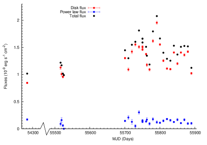
Figure 2.— Unabsorbed fluxes from the best-fit phenomenological diskbb+powerlaw models.

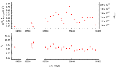
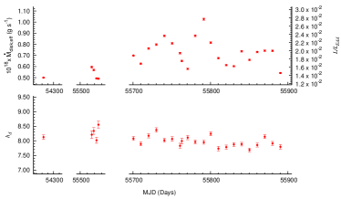
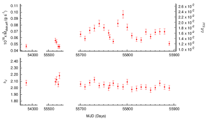
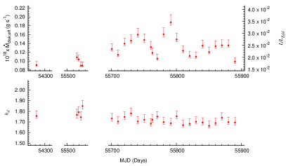
Figure 3.— Best-fit values assuming $M$=10M_⊙, $D$=10 kpc, and $i$=55°(top-left), 65°(top-right), 75°(bottom-left), and 85°(bottom-right). The top subpanel of each triplet shows the variation of $\dot{m}$ and Eddington fraction ($L/L_{\rm Edd}$) with time, and the bottom subpanel shows the variation of spectral hardening factor ($h_{d}$). The best-fit $h_{d}$ values for $i$=55° and 65° are clearly unphysical. The full set of figures showing the best-fit values as well as fitted and residual spectra for every observation for all the {M_BH, $d$, $i$} triplets explored in this paper can be seen online.

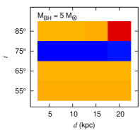
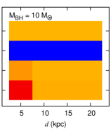
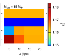
Figure 4.— Heat maps based on best-fit reduced-$\chi^{2}$ values. Each {M_BH, $d$, $i$} triplet is represented by a square whose color is indicative of the best-fit reduced-$\chi^{2}$ obtained by simultaneously fitting all 26 observations. The left, middle and right panels are for $M=5,10,15$M_⊙ respectively. Note that an inclination of $\sim$75° is preferred irrespective of the black hole’s assumed mass.

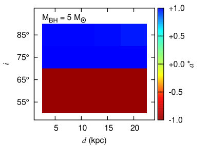
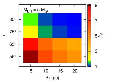
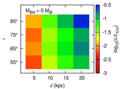
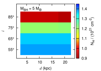
Figure 5.— Heat maps based on values of best-fit parameters, assuming M_BH=5M_⊙. The top-left, top-right, bottom-left, and bottom-right panels are for $a^{*}$, $h_{d}$, $L/L_{\rm Edd}$, and N_H respectively. For the top-left ($a^{*}$) and bottom-right (N_H) panels each {M_BH, $d$, $i$} triplet is represented by a square whose color is indicative of the best-fit parameter value obtained by simultaneously fitting all 26 observations. For the top-right ($h_{d}$) and bottom-left ($L/L_{\rm Edd}$) panels each {M_BH, $d$, $i$} triplet is represented by a square whose color is indicative of the average of 26 best-fit values obtained by simultaneously fitting all 26 observations. Note the following:
$a^{*}$ – The best-fit value of the spin parameter rapidly changes between lower inclinations (55°, 65°) and higher inclinations (75°, 85°). See text, especially §4, for details.
$h_{d}$ – Values of $h_{d}$ in the range of $\sim$1.5-2.5 are physically plausible, and indicated by green and yellow color. Low inclination models ($i=55\arcdeg,65\arcdeg$) are strongly disfavored because of the unphysically high values of $h_{d}$. For higher inclinations, the regions of ‘acceptable’ $h_{d}$ values move progressively from 5–10 kpc for $\sim$5M_⊙to higher distances for higher accretor masses.
$L/L_{\rm Edd}$ – The typical $L/L_{\rm Edd}$ luminosity range spanned by X-ray binaries in soft state is encompassed by yellow, green, and bluish colors in our color scheme for this figure. Luminosities close to Eddington would drive strong winds that are not seen in this system. Therefore high $L/L_{\rm Edd}$ are unlikely. Smaller distances ($\sim$5 kpc) are not favored by any choices of the mass because the best-fit luminosities are too low. Higher accretor masses would require higher distances for the luminosity to be in the comfort zone for a soft state X-ray binary.
N_H – Lower inclinations prefer higher columns. The range of N_H values is consistent with independent observations made with other instruments.

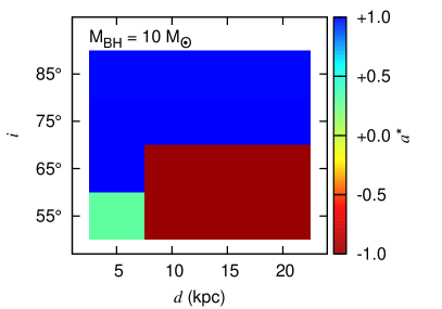
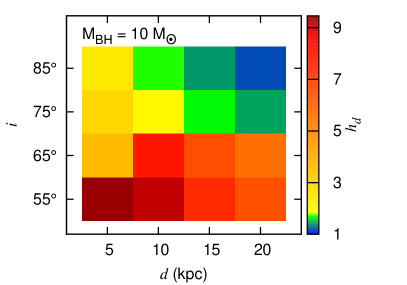
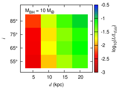
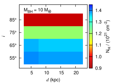
Figure 6.— Same as Fig. 5, but for M_BH=10M_⊙.

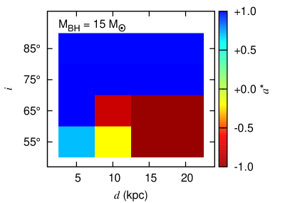
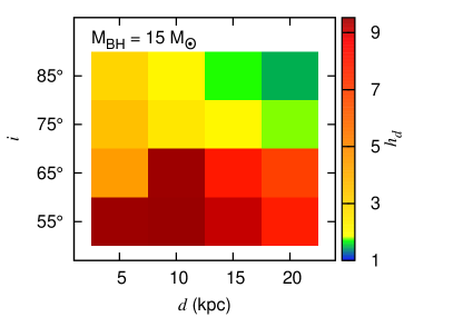
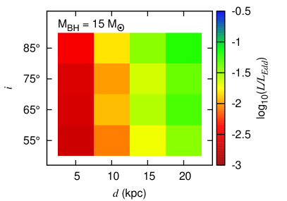
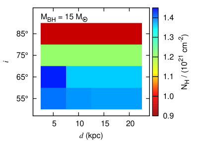
Figure 7.— Same as Fig. 5, but for M_BH=15M_⊙.

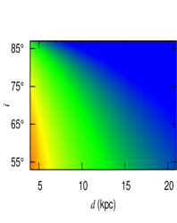
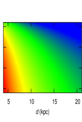
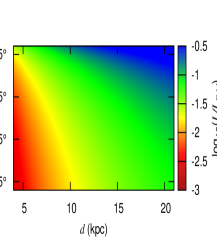
Figure 8.— Heat maps based on computing $L/L_{\rm Edd}$ assuming an isotropic source flux of 1.5$\times$10^-9 erg s^-1 cm^-2. The left, middle and right panels are for $M$ = 5, 10, and 15M_⊙ respectively.

Figure 9.— Residuals to the MCMC model with minimum $\chi^{2}$for the first 24 observations. The MJD of the observation is indicated in the top-right of every plot.

Figure 10.— Residuals to the MCMC model with minimum $\chi^{2}$for the last two observations. The MJD of the observation is indicated in the top-right of every plot.

	NH	$i$	$a^{*}$
NH
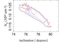
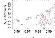
$i$
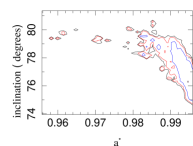
$a^{*}$

Figure 11.— MCMC results from a chain of 5,757,000 elements after rejecting data from the initial burn-in period. The marginalized 1D histograms along the diagonal panels clearly show a single-peaked distribution for N_H and $i$. On the other hand we can only obtain a lower limit on the spin parameter. The off-diagonal contour plots show the correlation between N_H, $i$, and $a^{*}$. For the contour plots, the blue, red, and black colors correspond to 68%, 90%, and 95% confidence contours.

References

- Abramowicz et al. (1978) Abramowicz, M., Jaroszynski, M., & Sikora, M. 1978, A&A, 63, 221
- Anders & Grevesse (1989) Anders, E., & Grevesse, N. 1989, Geochim. Cosmochim. Acta, 53, 197
- Arnaud (1996) Arnaud, K. A. 1996, Astronomical Data Analysis Software and Systems V, 101, 17
- Balucinska-Church & McCammon (1992) Balucinska-Church, M., & McCammon, D. 1992, ApJ, 400, 699
- Bardeen & Petterson (1975) Bardeen, J. M., & Petterson, J. A. 1975, ApJ, 195, L65
- Bayless et al. (2011) Bayless, A., Robinson, E., Mason, P., & Robertson, P. 2011, ApJ, 730, 43
- Burrows et al. (2005) Burrows D.N. et al., 2005, SSRev, 120, 165
- Davis et al. (2005) Davis, S. W., Blaes, O. M., Hubeny, I., & Turner, N. J. 2005, ApJ, 621, 372
- Foreman-Mackey et al. (2013) Foreman-Mackey D. et al., 2013, PASP, 125, 306
- Gehrels et al. (2004) Gehrels N. et al., 2004, ApJ, 611, 1005
- Giacconi et al. (1974) Giacconi, R., Murray, S., Gursky, H., Kellogg, E., Schreier, E., Matilsky, T., Koch, D., & Tananbaum, H. 1974, ApJS, 27, 37
- Goodman & Weare (2010) Goodman, J., & Weare, J. 2010, Commun. Appl. Math. Comput. Sci., 5, 65
- Houck & Denicola (2000) Houck, J. C., & Denicola, L. A. 2000, in ASP Conf. Ser. 216: Astronomical Data Analysis Software and Systems IX, Vol. 9, 591
- Li et al. (2005) Li, L.-X., Zimmerman, E. R., Narayan, R., & McClintock, J. E. 2005, ApJS, 157, 335
- Maccarone (2003) Maccarone, T. J., 2003, A&A, 409, 697
- Maitra et al. (2009) Maitra, D., Markoff, S., Brocksopp, C., et al. 2009, MNRAS, 398, 1638
- Mason et al. (2012) Mason, P. A., Robinson, E. L., Bayless, A. J., & Hakala, P. J. 2012, AJ, 144, 108
- McClintock et al. (2006) McClintock, J. E., Shafee, R., Narayan, R., et al. 2006, ApJ, 652, 518
- Misner et al. (1973) Misner, C. W., Thorne, K. S., & Wheeler, J. A. 1973, Gravitation (San Francisco, CA: Freeman)
- Mitsuda et al. (1984) Mitsuda, K., Inoue, H., Koyama, K., et al. 1984, PASJ, 36, 741
- Noble et al. (2006) Noble, M. S., Houck, J. C., Davis, J. E., Young, A., & Nowak, M. 2006, Astronomical Data Analysis Software and Systems XV, 351, 481
- Nowak et al. (2008) Nowak, M. A., Juett, A., Homan, J., et al. 2008, ApJ, 689, 1199
- Nowak et al. (2012) Nowak, M. A., Wilms, J., Pottschmidt, K., et al. 2012, ApJ, 744, 107
- Nowak & Wilms (1999) Nowak, M. A., & Wilms, J. 1999, ApJ, 522, 476
- Reynolds & Miller (2013) Reynolds, M., & Miller, J. 2013, ApJ, 769, 16
- Ricci et al. (1995) Ricci, D. and Israel, G. L. and Stella, L. 1995, A&A, 299, 731
- Robinson et al. (2012) Robinson, E. L., Bayless, A. J., Mason, P. A., & Robertson, P. 2012, American Astronomical Society Meeting Abstracts, 219, #153.13
- Russell et al. (2010) Russell, D., Lewis, F., Roche, P., Clark, J.S. Breedt, E., & Fender, R. 2010, MNRAS, 402, 2671
- Russell et al. (2011) Russell, D. M., Miller-Jones, J. C. A., Maccarone, T. J., et al. 2011, ApJ, 739, L19
- Sadowski et al. (2011) Sa̧dowski, A., Bursa, M., Abramowicz, M., et al. 2011, A&A, 532, 41
- Salvesen et al. (2013) Salvesen, G., Miller, J. M., Reis, R. C., & Begelman, M. C. 2013, MNRAS, 431, 3510
- Shafee et al. (2006) Shafee, R., McClintock, J. E., Narayan, R., et al. 2006, ApJ, 636, L113
- Shimura & Takahara (1995) Shimura, T., & Takahara, F. 1995, ApJ, 445, 780
- Singh et al. (1994) Singh, K. P., Apparao, K. M. V. & Kraft, R. P. 1994, ApJ, 421, 753
- Thorne (1974) Thorne, K. S., 1977, ApJ, 191, 507
- Thorstensen (1987) Thorstensen, J. R., 1987, ApJ, 312, 739
- Wijnands et al. (2002) Wijnands, R., Miller, J., & van der Klis, M. 2002, MNRAS, 331, 60
- Yan et al. (1998) Yan, M., Sadeghpour, H. R., & Dalgarno, A. 1998, ApJ, 496, 1044
- Yao et al. (2008) Yao, Y., Nowak, M. A., Wang, Q. D., Schulz, N. S., & Canizares, C. R. 2008, ApJ, 672, L21
- Yaqoob et al. (1993) Yaqoob, T., Ebisawa, K., & Mitsuda, K. 1993, MNRAS, 264, 411