Blind Calibration in Compressed Sensing using Message Passing Algorithms

Abstract

Compressed sensing (CS) is a concept that allows to acquire compressible signals with a small number of measurements. As such it is very attractive for hardware implementations. Therefore, correct calibration of the hardware is a central issue. In this paper we study the so-called blind calibration, i.e. when the training signals that are available to perform the calibration are sparse but unknown. We extend the approximate message passing (AMP) algorithm used in CS to the case of blind calibration. In the calibration-AMP, both the gains on the sensors and the elements of the signals are treated as unknowns. Our algorithm is also applicable to settings in which the sensors distort the measurements in other ways than multiplication by a gain, unlike previously suggested blind calibration algorithms based on convex relaxations. We study numerically the phase diagram of the blind calibration problem, and show that even in cases where convex relaxation is possible, our algorithm requires a smaller number of measurements and/or signals in order to perform well.

1 Introduction

The problem of acquiring an $N$-dimensional signal ${\bf x}$ through $M$ linear measurements, ${\bf y}=F{\bf x}$, arises in many contexts. The Compressed Sensing (CS) approach [1, 2] exploits the fact that, in many cases of interest, the signal is $K$-sparse (in an appropriate known basis), meaning that only $K=\rho N$ out of the $N$ components are non-zero. Compressed sensing theory shows that a $K$-sparse $N$-dimensional signal can be reconstructed from far less than $N$ linear measurements [1, 2], thus saving acquisition time, cost or increasing the resolution. In the most common setting, the linear $M\times N$ map $F$ is considered to be known.

Nowadays, the concept of compressed sensing is very attractive for hardware implementations. However, one of the main issues when building hardware revolves around calibration. Usually the sensors introduce a distortion (or decalibration) to the measurements in the form of some unknown gains. Calibration is about how to determine the transfer function between the measurements and the readings from the sensor. In some applications dealing with distributed sensors or radars for instance, the location or intrinsic parameters of the sensors are not exactly known [3, 4]. Similar distortion can be found in applications with microphone arrays [5]. The need for calibration has been emphasized in a number of other works, see e.g. [6, 7, 8]. One common way of dealing with calibration (apart from ignoring it or considering it as measurement noise) is supervised calibration when some known training signals ${\bf x}_{l}$, $l=1,\dots,P$ and the corresponding observations ${\bf y}_{l}$ are used to estimate the distortion parameters.

In the present work we are interested in blind (unsupervised) calibration, in which known training signals are not available, and one can only use unknown (but sparse) signals. If such calibration is computationally possible, then it might be simpler to do than the supervised calibration in practice .

1.1 Setting

We state the problem of blind calibration in the following way. First we introduce an unknown distortion parameter (we will also use equivalently the term decalibration parameter or gain) $d_{\mu}$ for each of the sensors, $\mu=1,\dots,M$. Note that $d_{\mu}$ can also represent a vector of several parameters. We consider that the signal is linearly projected by a known $M\times N$ measurement matrix $F$ and only then distorted according to some known transfer function $h$. This transfer function can be probabilistic (noisy), non-linear, etc. Each sensor $\mu$ then provides the following distorted and noisy reading (measure) $y_{\mu}=h(z_{\mu l},d_{\mu},w_{\mu})$ where $z_{\mu}=\sum_{i=1}^{N}F_{\mu i}x_{i}$ is the linear projection of the signal on the $\mu$th row of the measurement matrix $F$. For the measurement noise $w_{\mu}$, one usually one considers an iid Gaussian noise with variance $\Delta$ added to $z_{\mu}$.

In order to perform the blind calibration, we need to measure several statistically diverse signals. Given a set of $N$-dimensional $K$-sparse signals ${\bf x}_{l}$ with $l=1,\cdots,P$, for each of the signals we consider $M$ sensor readings

$$y_{\mu l}=h(z_{\mu l},d_{\mu},w_{\mu l})\,,\quad{\rm where}\quad z_{\mu l}=\sum_{i=1}^{N}F_{\mu i}x_{il}\,,$$ (1)

where $d_{\mu}$ are the signal-independent distortion parameters, $w_{\mu l}$ is a signal-dependent measurement noise, and $h$ is an arbitrary known function of these variables with standard regularity requirements. Given the $M\times P$ measurements $y_{\mu l}$ and a perfect knowledge of the matrix $F$, we want to infer both the $P$ different signals $\{{\bf x}_{1},\cdots{\bf x}_{P}\}$ and the $M$ distortion parameters $d_{\mu}$, $\mu=1,\cdots M$.

1.2 Relation to previous work

As far as we know, the problem of blind calibration was first studied in the context of compressed sensing in [9] where the distortions were considered as multiplicative, i.e. the transfer function was

$$h(z_{\mu l},d_{\mu},w_{\mu l})=\frac{1}{d_{\mu}}(z_{\mu l}+w_{\mu l})\,.$$ (2)

A subsequent work [10] considers a more general case when the distortion parameters are $d_{\mu}=(g_{\mu},\theta_{\mu})$, and the transfer function $h(z_{\mu l},d_{\mu},w_{\mu l})=e^{i\theta_{\mu}}(z_{\mu l}+w_{\mu l})/g_{\mu}$. Both [9] and [10] applied convex optimization based algorithms to the blind calibration problem and their approach seems to be limited to the above special cases of transfer functions. Our approach is able to deal with a general transfer function $h$, and moreover for the product-transfer-function (2) it outperforms the algorithm of [9].

The most commonly used algorithm for signal reconstruction in compressed sensing is the $\ell_{1}$ minimization of [1]. In compressed sensing without noise and for measurement matrices with iid Gaussian elements, the $\ell_{1}$ minimization algorithm leads to exact reconstruction as long as the measurement rate $\alpha=M/N>\alpha_{\rm DT}$ in the limit of large signal dimension, where $\alpha_{\rm DT}$ is a well known phase transition of Donoho and Tanner [11]. The blind calibration algorithm of [9, 10] also directly uses $\ell_{1}$ minimization for reconstruction.

In the last couple of years, the theory of compressed sensing witnessed a large progress thanks to the development of message passing algorithms based on the standard loopy Belief Propagation (BP) and their analysis [12, 13, 14, 15, 16]. In the context of compressed sensing, the canonical loopy BP is difficult to implement because its messages would be probability distributions over a continuous support. At the same time in problems such as compressed sensing, Gaussian or quadratic approximation of BP still contains the information necessary for a successful reconstruction of the signal. Such approximations of loopy BP originated in works on CDMA multiuser detection [17, 18]. In compressed sensing the Gaussian approximation of BP is known as the approximate message passing (AMP) [12, 13], and it was used to prove that with properly designed measurement matrices $F$ the signal can be reconstructed for measurement rate as low as $\alpha=\rho$ asymptotically, thus closing the gap between the Donoho-Tanner transition and the information theoretical lower bound [15, 16]. Even without particular design of the measurement matrices the AMP algorithm outperforms the $\ell_{1}$-minimization for a large class of signals. Importantly for the present work, [14] generalized the AMP algorithm to deal with a wider range of input and output functions. For some of those, generalizations of the $\ell_{1}$-minimization based approach are not convex anymore, and hence they do not have the advantage of provable computational tractability anymore.

The following two works have considered blind calibration related problems with the use if AMP-like algorithms. In [19] the authors use AMP combined with expectation maximization to calibrate gains that act on the signal components rather than on the measurement components as we consider here. In [20] the authors study the case when every element of the measurement matrix $F$ has to be calibrated, in contrast to the row-constant gains considered in this paper. The setting of [20] is much closer to the dictionary learning problem and is much more demanding, both computationally and in terms of the number of different signals necessary for successful calibration.

1.3 Contributions

In this work we extend the generalized approximate message passing (GAMP) algorithm of [14] to the problem of blind calibration with a general transfer function $h$, eq. (1). We denote it as the calibration-AMP or C-AMP algorithm. The C-AMP uses $P>1$ unknown sparse signals to learn both the different signals ${\bf x}_{l}$, $l=1,\dots,P$, and the distortion parameters $d_{\mu}$, $\mu=1,\dots,M$, of the sensors. We hence overcome the limitations of the blind calibration algorithm presented in [9, 10] to the class of settings for which the calibration can be written as a convex optimization problem.

In the second part of this paper we analyze the performance of C-AMP for the product transfer function (2) used in [9] and demonstrate its scalability and better performance with respect to their $\ell_{1}$-based approach. In the numerical study we observe a sharp phase transition generalizing the phase transition seen for AMP in compressed sensing [21]. Note that for the blind calibration problem to be solvable, we need the amount of information contained in the sensor readings, $PM$, to be at least as large as the size of the vector of distortion parameters $M$, plus the number of the non-zero components of all the signals, $KP$. Defining $\rho=K/N$ and $\alpha=M/N$, this leads to $\alpha P\geq\rho P+\alpha$. If we fix the number of signals $P$ we have a well defined line in the $(\rho,\alpha)$-plane given by

$$\alpha\geq\frac{P}{P-1}\rho\equiv\alpha_{\rm min}\,,$$ (3)

below which exact calibration cannot be possible. We will compare the empirically observed phase transition to this theoretical bound as well as to the phase transition that would have been observed in the pure compressed sensing, i.e. if we knew the distortion parameters.

2 The Calibration-AMP algorithm

The approximate message passing algorithm is based on a Bayesian probabilistic formulation of the reconstruction problem. Denoting $P_{X}(x_{il})$ the assumed empirical distribution of the components of the signal, $P_{W}(w_{\mu l})$ the assumed probability distribution of the components of the noise, and $P_{D}(d_{\mu})$ the assumed empirical distribution of the distortion parameters, the Bayes formula yields

$$P({\bf x},{\bf d}|{\bf F},{\bf y})=\frac{1}{Z}\prod_{i,l=1}^{N,P}P_{X}(x_{il})\,\prod_{\mu=1}^{M}P_{D}(d_{\mu})\prod_{l,\mu=1}^{P,M}\int\,dw_{\mu l}P_{W}(w_{\mu l})\delta\left[y_{\mu l}-h\left(z_{\mu l},d_{\mu},w_{\mu l}\right)\right]\,,$$ (4)

where $Z$ is a normalization constant and $z_{\mu l}=\sum_{i}F_{\mu i}x_{il}$. We denote the marginals of the signal components $\nu^{x}_{il}(x_{il})=\int\prod_{\mu}{\rm d}d_{\mu}\prod_{jn\neq il}dx_{jn}\,P({\bf x},{\bf d}|{\bf F},{\bf y})$ and those of the distortion parameters $\nu^{x}_{il}(x_{il})=\int\prod_{\mu}{\rm d}d_{\mu}\prod_{jn\neq il}dx_{jn}\,P({\bf x},{\bf d}|{\bf F},{\bf y})$. The estimators $x^{*}_{il}$ that minimizes the expected mean-squared error (MSE) of the signals and the estimator $d^{*}_{\mu}$ of the distortion parameters are the averages w.r.t. the marginal distributions, namely $x^{*}_{il}=\int{\rm d}x_{il}\,x_{il}\,\nu^{x}_{il}(x_{il})$ and $d^{*}_{\mu}=\int{\rm d}d_{\mu}\,d_{\mu}\,\nu^{d}_{\mu}(d_{\mu})$. An exact computation of these estimates is not tractable in any known way so we use instead a belief-propagation based approximation that has proven to be fast and efficient in the compressed sensing problem [12, 13, 14].

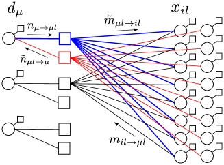
Figure 1: Graphical model representing the blind calibration problem. Here the dimensionality of the signal is $N\!=\!8$, the number of sensors is $M\!=\!3$, and the number of signals used for calibration $P\!=\!2$. The variable nodes $x_{il}$ and $d_{\mu}$ are depicted as circles, the factor nodes as squares.

Given the factor graph representation of the calibration problem in Fig. 1, the canonical belief propagation equations for the probability measure (4) are written in terms of $NPM$ messages $\tilde{m}_{\mu l\rightarrow il}(x_{il})$, and $m_{il\rightarrow\mu l}(x_{il})$ representing probability distributions on the signal component $x_{il}$, and $PM$ messages $n_{\mu\rightarrow\mu l}$ and $\tilde{n}_{\mu l\rightarrow\mu}$ representing probability distributions on the distortion parameter $d_{\mu}$. Following the lines of [12, 13, 14, 15], with the use of the central limit theorem, a Gaussian approximation, and neglecting terms that go to zero as $N\rightarrow\infty$, the BP equations can be closed using only the means $a_{il\rightarrow\mu l}=\int{\rm d}x_{il}\,m_{il\rightarrow\mu l}(x_{il})\,x_{il}$ and variances $v_{il\rightarrow\mu l}=\int{\rm d}x_{il}\,m_{il\rightarrow\mu l}(x_{il})\,x^{2}_{il}-a^{2}_{il\rightarrow\mu l}$ of the above messages $m_{il\rightarrow\mu l}$ and the means $k_{\mu\rightarrow\mu l}=\int{\rm d}d_{\mu}\,n_{\mu\rightarrow\mu l}(d_{\mu})\,d_{\mu}$ and variances $l_{\mu\rightarrow\mu l}=\int{\rm d}d_{\mu}\,n_{\mu\rightarrow\mu l}(d_{\mu})\,d^{2}_{\mu}-k^{2}_{\mu\rightarrow\mu l}$ of the above messages $n_{\mu\rightarrow\mu l}$. Moreover, again neglecting only terms that go to zero as $N\rightarrow\infty$, we can write closed equations on quantities that correspond to the variables and factors nodes, instead of messages running between variables and factor nodes. For this we introduce $\omega_{\mu l}=\sum_{i}F_{\mu i}a_{il\rightarrow\mu l}$ and $V_{\mu l}=\sum_{i}F^{2}_{\mu i}v_{il\rightarrow\mu l}$. The derivation of the C-AMP algorithm goes very much along the lines of [12, 13, 14, 15]. To summarize the resulting algorithm we define the “generating function” $G$ as

$$G(y_{\mu\cdot},\omega_{\mu\cdot},V_{\mu\cdot},\theta)=\ln\left[\int{\rm d}d\,P_{D}(d)\,\prod_{n=1}^{P}\tilde{G}(y_{\mu n},d,\omega_{\mu n},V_{\mu n})\,e^{\theta d}\right]\,,$$ (5)

where

$$\tilde{G}(y,d,\omega,v)=\int{\rm d}z\,{\rm d}w\,P_{W}(w)\,\delta[h(z,d,w)-y]\,e^{-\frac{1}{2}\frac{(z-\omega)^{2}}{v}}\,,$$ (6)

where $\mu\cdot$ indicates a dependence on all the variables labeled $\mu n$ with $n=1,\cdots,P$, and $\delta(\cdot)$ is the Dirac delta function. Similarly as Rangan in [14], we define $P$ output functions as

$$g^{l}_{\mathrm{out}}(y_{\mu\cdot},\omega_{\mu\cdot},V_{\mu\cdot})=\frac{\partial}{\partial\omega_{\mu l}}G(y_{\mu\cdot},\omega_{\mu\cdot},V_{\mu\cdot},\theta=0)\,.$$ (7)

Note that each of the output functions depend on all the $P$ different signals. We also define the following input functions

$$f^{x}_{a}(\Sigma^{2},R)=[x]_{X}\,,\quad\quad f^{x}_{c}(\Sigma^{2},R)=[x^{2}]_{X}-[x]_{X}^{2}\,,$$ (8)

where $[\dots]_{X}$ indicates expectation w.r.t. the measure

$${\cal M}_{X}(x,\Sigma^{2},R)=\frac{1}{Z(\Sigma^{2},R)}P_{X}(x)\,\,e^{-\frac{(x-R)^{2}}{2\Sigma^{2}}}\,.$$ (9)

Given the above definitions, the iterative calibration-AMP algorithm reads as follows

$$V^{t+1}_{\mu l} = \sum_{i}F_{\mu i}^{2}\,v^{t}_{il}\,,$$ (10)

$$e^{t+1}_{\mu l} = g^{l}_{\mathrm{out}}(y_{\mu\cdot},\omega^{t}_{\mu\cdot},V^{t+1}_{\mu\cdot})\,,$$ (11)

$$h^{t+1}_{\mu l} = -\frac{\partial}{\partial\omega_{\mu l}}g^{l}_{\mathrm{out}}(y_{\mu\cdot},\omega^{t}_{\mu\cdot},V^{t+1}_{\mu\cdot})\,,$$ (12)

$$\omega^{t+1}_{\mu l} = \sum_{i}F_{\mu i}a^{t}_{il}-V^{t+1}_{\mu l}\,e^{t+1}_{\mu l}\,,$$ (13)

$$(\Sigma^{t+1}_{il})^{2}=\left[\sum_{\mu}F_{\mu i}^{2}\,h^{t+1}_{\mu l}\right]^{-1}\,,~{} ~{}~{}~{}R^{t+1}_{il}=a_{il}+\left[\sum_{\mu}F_{\mu i}\,e^{t+1}_{\mu l}\right](\Sigma^{t+1}_{il})^{2}\,,$$ (14)

$$a^{t+1}_{il}=f^{x}_{a}((\Sigma^{t+1}_{il})^{2},R^{t+1}_{il})\,,~{} ~{}~{}~{}v^{t+1}_{il}=f^{x}_{c}((\Sigma^{t+1}_{il})^{2},R^{t+1}_{il})\,,$$ (15)

we initialize $\omega_{\mu l}^{t=0}=y_{\mu l}$, $a^{t=0}_{il}$ and $v_{il}^{t=0}$ as the mean and variance of the assumed distribution $P_{X}(\cdot)$, and iterate these equations until convergence. At every time-step the quantity $a_{il}$ is the estimate for the signal element $x_{il}$, and $v_{il}$ is the approximate error of this estimate. The estimate and its error for the distortion parameter $d_{\mu}$ can be computed as

$$k^{t+1}_{\mu} = \frac{\partial}{\partial\theta}G(y^{t+1}_{\mu\cdot},\omega^{t+1}_{\mu\cdot},V^{t+1}_{\mu\cdot},\theta)\Big{|}_{\theta=0}\,,$$ (16)

$$l^{t+1}_{\mu} = \frac{\partial^{2}}{\partial\theta^{2}}G(y^{t+1}_{\mu\cdot},\omega^{t+1}_{\mu\cdot},V^{t+1}_{\mu\cdot},\theta)\Big{|}_{\theta=0}\,.$$ (17)

By setting $P_{D}(d_{\mu})=\delta(d_{\mu}-d_{\mu}^{\rm true})$, and simplifying eq. (5), readers familiar with the work of Rangan [14] will recognize the GAMP algorithm in eqs. (10-15). Note that for a general transfer function $h$ the generating function $G$ (5) has to be evaluated numerically. The overall running time of the C-AMP algorithm is comparable to the one of GAMP [14], it is hence very scalable.

2.1 C-AMP for the product transfer function

In the numerical section of this paper we will focus on a specific case of the transfer function $h(z_{\mu l},d_{\mu},w_{\mu l})$, defined in eq. (2). We consider the measurement noise $w_{\mu l}$ to be Gaussian of zero mean and variance $\Delta$. This transfer function was considered in the work of [9] and we will hence be able to compare the performance of C-AMP directly to the convex optimization investigated in [9]. For the product transfer function eq. (2) most integrals requiring a numerical computation in the general case are expressed analytically and C-AMP becomes (together with eqs. (10) and (13-15):

$$e^{t+1}_{\mu l} = \frac{k^{t}_{\mu}y_{\mu l}-\omega^{t}_{\mu l}}{V^{t+1}_{\mu l}+\Delta}\,,$$ (18)

$$h^{t+1}_{\mu l} = \frac{1}{V^{t+1}_{\mu l}+\Delta}-\frac{l^{t}_{\mu}y_{\mu l}^{2}}{(V^{t+1}_{\mu l}+\Delta)^{2}}\,,$$ (19)

$$k^{t+1}_{\mu} = f^{d}_{a}((C^{t+1}_{\mu})^{2},T^{t+1}_{\mu})\,,$$ (20)

$$l^{t+1}_{\mu} = f^{d}_{c}((C^{t+1}_{\mu})^{2},T^{t+1}_{\mu})\,,$$ (21)

$$(C^{t+1}_{\mu})^{2} = \left[\sum_{n}\frac{y_{\mu n}^{2}}{V^{t+1}_{\mu n}+\Delta}\right]^{-1}\,,$$ (22)

$$T^{t+1}_{\mu} = (C^{t+1}_{\mu})^{2}\,\sum_{n}\frac{y_{\mu n}\omega^{t+1}_{\mu n}}{V^{t+1}_{\mu n}+\Delta}\,.$$ (23)

where we have introduced

$$f^{d}_{a}(C^{2},T)=[d]_{D}\,,\quad\quad f^{d}_{c}(C^{2},T)=[d^{2}]_{D}-[d]_{D}^{2}\,,$$ (24)

with $[\dots]_{D}$ indicating the expectation w.r.t. the measure

$${\cal M}_{D}(d,C^{2},T)=\frac{1}{Z(C^{2},T)}P_{D}(d)|d|^{P}\,\,e^{-\frac{(d-T)^{2}}{2C^{2}}}\,.$$ (25)

3 Experimental results

Our simulations were performed using a MATLAB implementation of the C-AMP algorithm presented in the previous section, that is available online. We focused on the noiseless case $\Delta=0$ for which, when there is no distortion of the output, exact reconstruction of the signal is possible. We tested the algorithm on randomly generated Gauss-Bernoulli signals with density of non-zero elements $\rho$, their distribution being a Gaussian one with zero mean and unit variance. For the present experiments the algorithm is using this information via a matching distribution $P_{X}(x_{il})$. The situation when $P_{X}$ mismatches the true signal distribution was discussed for AMP for compressed sensing in [21].

The distortion parameters $d_{\mu}$ were generated from a uniform distribution centered at $d=1$ having variance $\sigma^{2}$. This ensures that, as $\sigma^{2}\rightarrow 0$, the results of standard compressed sensing are recovered, while the distortions are more and more serious as $\sigma^{2}$ is growing. For numerical stability purposes, the variance of the assumed distribution of the distortions used in the update functions of C-AMP was taken to be slightly larger than the variance used to create the actual distortion parameters. For the same reasons, we have also added a small noise $\Delta=10^{-17}$ and used a damping factor in the iterations in order to avoid oscillatory behavior. In this noiseless case we iterate the C-AMP equations until the following quantity ${\rm crit}=\frac{1}{MP}\sum_{\mu l}\left(k_{\mu}y_{\mu l}-\sum_{i}F_{\mu i}a_{il}\right)^{2}$ becomes smaller than the numerical precision of implementation (in case of perfect recovery), around $10^{-16}$, or until that quantity does not decrease any more over 100 iterations (when a fixed point is reached, but the reconstruction is not perfect).

Success or failure of the reconstruction is usually determined by looking at the mean squared error (MSE) between the true signal $\bf x_{l}^{0}$ and the reconstructed ones $\bf a_{l}$. In the noiseless setting the product transfer function $h$ leads to a scaling invariance: if $\bf x_{l}^{0}$ and $\bf d^{0}$ are the true signals and the true distortion parameters, multiplying both by the same non-zero real number $s$ leads to another possible solution of the system. Therefore, a better measure of success is the cross-correlation between real and recovered signal (used in [10]) or a corrected version of the MSE, defined by:

$${\rm MSE}^{\rm corr}=\frac{1}{NP}\sum_{il}\left(x_{il}^{0}-\hat{s}a_{il}\right)^{2}\,,\quad{\rm where}\quad\hat{s}=\frac{1}{M}\sum_{\mu}\frac{d^{0}_{\mu}}{k_{\mu}}$$ (26)

is an estimation of the scaling factor $s$. Slight deviations between empirical and theoretical means due to the finite size of $M$ and $N$ lead to important differences between ${\rm MSE}$ and ${\rm MSE}^{\rm corr}$, only the latter going truly to zero for finite $N$ and $M$.

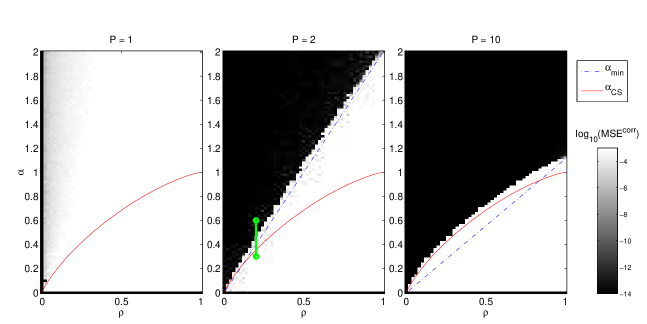
Figure 2: Phase diagrams for different numbers $P$ of calibrating signals: The measurement rate $\alpha=M/N$ is plotted against the density of the signal $\rho=K/N$. The plotted value is the decimal logarithm of the corrected mean squared error (26) achieved for one randomly chosen instance. White indicates failure of the reconstruction, while black represents perfect reconstruction (i.e. a MSE of the order of the numerical precision). In this figure the distortion variance is $\sigma^{2}=0.01$ and $N=1000$. While for $P\!=\!1$ reconstruction is never possible, for $P\!>\!1$, there is a phase transition very close to the lower bound defined by $\alpha_{\rm min}$ in equation (3) or to the phase transition line of the pure compressed sensing problem $\alpha_{\rm CS}$. Note that while this diagram is usually plotted only for $\alpha\leq 1$ for compressed sensing, the part $\alpha>1$ displays pertinent information in blind calibration.

Fig. 2 shows the empirical phase diagrams in the $\alpha$-$\rho$ plane we obtained from the C-AMP algorithm for different number of signals $P$. For $P=1$ the reconstruction is never exact, whereas for any $P>1$, there is a sharp phase transition taking place with a jump in ${\rm MSE}^{\rm corr}$ of ten orders of magnitude. As $P$ increases, the phase of exact reconstruction gets bigger and tends to the one observed in Bayesian compressed sensing when no distortion of the output is present [15]. Remarkably, for small values of the density $\rho$, the position of the C-AMP phase transition is very close to the compressed sensing one already for $P=2$ and C-AMP performs almost as well as in the absence of distortion.

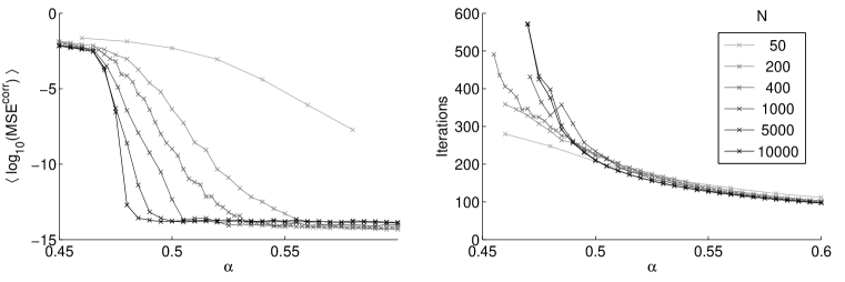
Figure 3: Left: C-AMP phase transition as the system size $N$ grows. The curves are obtained by averaging $\log_{10}({\rm MSE}^{\rm corr})$ over $100$ samples, reflecting the probability of correct reconstruction in the region close to the phase transition, where it is not guaranteed. Parameters are: $\rho=0.2$, $P=2$, $\sigma^{2}=0.0251$. For higher values of $N$, the phase transition becomes sharper. Right: Mean number of iterations necessary for reconstruction, when the true signal is successfully recovered. Far from the phase transition, increasing $N$ does not increase visibly the number of iterations for these system sizes, showing that our algorithm works in linear time. The number of needed iterations increases drastically as one approaches the phase transition.

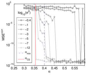
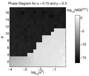
Figure 4: Left: Position of the phase transition in $\alpha$ for different distortion variances $\sigma^{2}$. The left vertical line represents the position of the compressed sensing phase transition, the right one is the counting bound eq. (3). With growing distortion, larger measurement rates become necessary for perfect calibration and reconstruction. Intermediary values of ${\rm MSE}^{\rm corr}$ are obtained in a region where perfect calibration is not possible, but distortions are small enough for the uncalibrated AMP to make only small mistakes. The parameters are those of Fig. 2, and $\alpha$ takes values on the green segment plotted on the $P=2$ diagram. Right: Phase diagram as the variance of the distortions $\sigma^{2}$ and the number of signals $P$ vary, for $\rho=0.5$, $\alpha=0.75$ and $N=1000$.

Fig. 3 shows the behavior near the phase transition, giving insights about the influence of the system size and the number of iterations needed for precise calibration and reconstruction. In Fig. 4, we show the jump in the MSE on a single instance as the measurement rate $\alpha$ decreases. The right part is the phase diagram in the $\sigma^{2}$-$P$ plane.

In [9, 10], a calibration algorithm using $\ell_{1}$-minimization have been proposed. While in that case, no assumption on the distribution of the signals and of the the gains is needed, for most practical cases it is expected to be less performant than the C-AMP if these distributions are known or reasonably approximated. We implemented the algorithm of [9] with MATLAB using the CVX package [22]. Due to longer running times, experiments were made using a smaller system size $N=100$. We also remind at this point that whereas the C-AMP algorithm works for a generic transfer function (1), the $\ell_{1}$-minimization based calibration is restricted to the transfer functions considered by [9, 10]. Fig. 5 shows a comparison of the performances of the two algorithms in the $\alpha$-$\rho$ phase diagrams. The C-AMP clearly outperforms the $\ell_{1}$-minimization in the sense that the region in which calibration is possible is much larger.

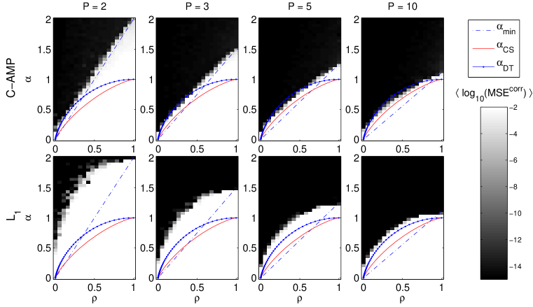
Figure 5: Comparison of the empirical phase diagrams obtained with the C-AMP algorithm proposed here (top) and the $\ell_{1}$-minimization algorithm of [9] (bottom) averaged over several random samples; white indicates failure, black indicates success. The area where reconstruction is possible is consistently much larger for C-AMP than for $\ell_{1}$-minimization. The plotted lines are the phase transitions for the pure compressed sensing problem with the AMP algorithm ($\alpha_{CS}$, in red, from [21]), and with $\ell_{1}$-minimization (the Donoho-Tanner transition $\alpha_{\rm DT}$, in blue, from [11]). The line $\alpha_{\rm min}$ is the lower counting bound from eq. (3). The advantage of C-AMP over $\ell_{1}$-minimization is clear. Note that in both cases, the region close to the transition is blurred due to finite system size, hence a region of grey pixels (again, the effect is more prononced for the $\ell_{1}$ algorithm).

4 Conclusion

We have presented the C-AMP algorithm for blind calibration in compressed sensing, a problem where the outputs of the measurements are distorted by some unknown gains on the sensors, eq. (1). The C-AMP algorithm allows to jointly infer sparse signals and the distortion parameters of each sensor even with a very small number of signals and is computationally comparable to the GAMP algorithm [14]. Another advantage w.r.t. previous works is that the C-AMP algorithm works for generic transfer function between the measurements and the readings from the sensor, not only those that permit a convex formulation of the inference problem as in [9, 10]. In the numerical analysis, we focussed on the case of the product transfer function (2) studied in [9]. Our results show that, for the chosen parameters, calibration is possible with a very small number of different sparse signals $P$ (i.e. $P=2$ or $P=3$), even very close to the absolute minimum of measurements required by a counting bound (3). Comparison with the $\ell_{1}$-minimizing algorithm clearly shows lower requirements on the measurement rate $\alpha$ and on the number of signals $P$ for C-AMP. The C-AMP algorithm for blind calibration is scalable and simple to implement. The efficiency of blind (unsupervised) calibration for compressed sensing shows that the knowledge of the training signals is not necessary. We expect C-AMP to become useful in practical compressed sensing implementations.

Asymptotic analysis of the C-AMP algorithm can be done using the state evolution approach [12]. In the present case of blind calibration, however, the resulting equations include a $P$-uple integration that is numerically demanding and has hence been postponed to future work. Future work also includes the study of the robustness to the mismatch between assumed and true distribution of signal elements and distortion parameters, as well as the expectation-maximization based learning of the various parameters. Finally, the use of spatially coupled measurement matrices [15, 16] could further improve the performance of the algorithm and make the phase transition coincide with the information-theoretical counting bound (3).

References

- [1] E. J. Candès and T. Tao. Decoding by linear programming. IEEE Trans. Inform. Theory, 51:4203, 2005.
- [2] D. L. Donoho. Compressed sensing. IEEE Trans. Inform. Theory, 52:1289, 2006.
- [3] B. C. Ng and C. M. S. See. Sensor-array calibration using a maximum-likelihood approach. IEEE Transactions on Antennas and Propagation, 44(6):827–835, 1996.
- [4] Z. Yang, C. Zhang, and L. Xie. Robustly stable signal recovery in compressed sensing with structured matrix perturbation. IEEE Transactions on Signal Processing, 60(9):4658–4671, 2012.
- [5] R. Mignot, L. Daudet, and F. Ollivier. Compressed sensing for acoustic response reconstruction: Interpolation of the early part. In IEEE Workshop on Applications of Signal Processing to Audio and Acoustics (WASPAA), pages 225–228, 2011.
- [6] T. Ragheb, J. N Laska, H. Nejati, S. Kirolos, R. G Baraniuk, and Y. Massoud. A prototype hardware for random demodulation based compressive analog-to-digital conversion. In 51st Midwest Symposium on Circuits and Systems (MWSCAS), pages 37–40. IEEE, 2008.
- [7] J. A Tropp, J. N. Laska, M. F. Duarte, J. K Romberg, and R. G. Baraniuk. Beyond nyquist: Efficient sampling of sparse bandlimited signals. IEEE Trans. Inform. Theory, 56(1):520–544, 2010.
- [8] P. J. Pankiewicz, T. Arildsen, and T. Larsen. Model-based calibration of filter imperfections in the random demodulator for compressive sensing. arXiv:1303.6135, 2013.
- [9] R. Gribonval, G. Chardon, and L. Daudet. Blind calibration for compressed sensing by convex optimization. In IEEE International Conference on Acoustics, Speech and Signal Processing (ICASSP), pages 2713 – 2716, 2012.
- [10] C. Bilen, G. Puy, R. Gribonval, and L. Daudet. Blind sensor calibration in sparse recovery using convex optimization. In 10th Int. Conf. on Sampling Theory and Applications, 2013.
- [11] D. L. Donoho and J. Tanner. Sparse nonnegative solution of underdetermined linear equations by linear programming. Proc. Natl. Acad. Sci., 102(27):9446–9451, 2005.
- [12] D. L. Donoho, A. Maleki, and A. Montanari. Message-passing algorithms for compressed sensing. Proc. Natl. Acad. Sci., 106(45):18914–18919, 2009.
- [13] D.L. Donoho, A. Maleki, and A. Montanari. Message passing algorithms for compressed sensing: I. motivation and construction. In IEEE Information Theory Workshop (ITW), pages 1 –5, 2010.
- [14] S. Rangan. Generalized approximate message passing for estimation with random linear mixing. In Proc. of the IEEE Int. Symp. on Inform. Theory (ISIT), pages 2168 –2172, 2011.
- [15] F. Krzakala, M. Mézard, F. Sausset, Y.F. Sun, and L. Zdeborová. Statistical physics-based reconstruction in compressed sensing. Phys. Rev. X, 2:021005, 2012.
- [16] D. L. Donoho, A. Javanmard, and A. Montanari. Information-theoretically optimal compressed sensing via spatial coupling and approximate message passing. In Proc. of the IEEE Int. Symposium on Information Theory (ISIT), pages 1231–1235, 2012.
- [17] J. Boutros and G. Caire. Iterative multiuser joint decoding: Unified framework and asymptotic analysis. IEEE Trans. Inform. Theory, 48(7):1772–1793, 2002.
- [18] Y. Kabashima. A cdma multiuser detection algorithm on the basis of belief propagation. J. Phys. A: Math. and Gen., 36(43):11111, 2003.
- [19] U. S. Kamilov, A. Bourquard, E. Bostan, and M. Unser. Autocalibrated signal reconstruction from linear measurements using adaptive gamp. online preprint, 2013.
- [20] F. Krzakala, M. Mézard, and L. Zdeborová. Phase diagram and approximate message passing for blind calibration and dictionary learning. arXiv:1301.5898, 2013.
- [21] F. Krzakala, M. Mézard, F. Sausset, Y.F. Sun, and L. Zdeborová. Probabilistic reconstruction in compressed sensing: Algorithms, phase diagrams, and threshold achieving matrices. J. Stat. Mech., P08009, 2012.
- [22] M. Grant and S. Boyd. CVX: Matlab software for disciplined convex programming, version 2.0 beta. http://cvxr.com/cvx, 2012.