Micro- and macroturbulence predictions from CO5BOLD 3D stellar atmospheres

Abstract

We present an overview of the current status of our efforts to derive the microturbulence and macroturbulence parameters ($\xi_{\rm mic}$ and $\xi_{\rm mac}$) from the CIFIST grid of CO5BOLD 3D model atmospheres as a function of the basic stellar parameters $T\rm_{eff}$, $\log g$, and [M/H]. The latest results for the Sun and Procyon show that the derived microturbulence parameter depends significantly on the numerical resolution of the underlying 3D simulation, confirming that ‘low-resolution’ models tend to underestimate the true value of $\xi_{\rm mic}$. Extending the investigation to $12$ further simulations with different $T\rm_{eff}$, $\log g$, and [M/H], we obtain a first impression of the predicted trend of $\xi_{\rm mic}$ over the Hertzsprung-Russell diagram: in agreement with empirical evidence, microturbulence increases towards higher effective temperature and lower gravity. The metallicity dependence of $\xi_{\rm mic}$ must be interpreted with care, since it also reflects the deviation between the 1D and 3D photospheric temperature stratifications that increases systematically towards lower [M/H].

1 Introduction

In the context of classical spectrum analysis based on 1D model atmospheres, the auxiliary parameters micro- and macroturbulence ($\xi_{\rm mic}$ and $\xi_{\rm mac}$) play an important role. One of the great advantages of 3D hydrodynamical model atmospheres is their physically consistent thermal structure and velocity field, properly taking into account the effect of convective flows, overshoot, and waves. Based on first principles without free parameters, 3D stellar atmosphere models can be used to derive $\xi_{\rm mic}$ and $\xi_{\rm mac}$ from their hydrodynamical velocity fields. Even if these classical turbulence parameters are not relevant when using 3D model atmospheres for spectroscopic work, their knowledge can be useful. On the one hand, such results can be compared with empirical data obtained from classical 1D studies to check the validity of the 3D models. On the other hand, the predictions of the 3D models can be used to fix $\xi_{\rm mic}$ and $\xi_{\rm mac}$ in 1D spectroscopic work when an empirical determination of these parameters is not possible, due to a lack of microturbulence-sensitive lines (e.g. in low-resolution spectra of very metal-poor stars), or due to the ambiguity between macroturbulence and rotational line broadening.

In the following, we review the different methods we have used so far to derive the parameters $\xi_{\rm mic}$ (and subsequently $\xi_{\rm mac}$) from our 3D model atmospheres, and give an update of the relevant results. Our investigations are mainly focused on the Sun ($T\rm_{eff}$=5780 K, $\log g$=4.44, [M/H]=0) and Procyon ($T\rm_{eff}$=6500 K, $\log g$=4.0, [M/H]=0), where we have also studied the influence of the spatial resolution of the 3D numerical simulations on the derived turbulence parameters. Based on $12$ further simulations with different $T\rm_{eff}$, $\log g$, and [M/H], we finally report first preliminary results of an investigation in progress aiming at the prediction of the variation of $\xi_{\rm mic}$ over the Hertzsprung-Russell diagram (HRD). All 3D model atmospheres used for this investigation are taken from the CIFIST 3D model atmosphere grid (Ludwig et al., 2009) computed with CO5BOLD (Freytag et al., 2012).

2 Derivation of $\xi_{\rm mic}$ and $\xi_{\rm mac}$ from 3D model atmospheres

The different methods we have used to derive the turbulence parameters $\xi_{\rm mic}$ and $\xi_{\rm mac}$ from 3D hydrodynamical model atmospheres have been introduced by Steffen et al. (2009). We give a brief summary of the relevant points here.

2.1 Microturbulence

For simplicity, and in line with common practice, all methods assume that the small-scale photospheric velocity field may be described by an isotropic Gaussian probability distribution of the line-of-sight velocity, $P(v)$ $\sim$ $\exp(-v^{2}/\xi_{\rm mic}^{2})$, characterized by a single, depth-independent parameter, $\xi_{\rm mic}$. Basically, the value of $\xi_{\rm mic}$ is inferred from its effect on the equivalent width ($W$) of synthetic spectral lines, not from its influence on the shape of the line profiles.

Method 1 (M1) relies only on the 3D model, and yields a value of $\xi_{\rm mic}$ for any individual spectral line, thus allowing to map $\xi_{\rm mic}$ as a function of line strength $W$ and/or excitation potential $E_{i}$ for arbitrary ions. In principle, this method can also be employed to map a possible depth-dependence of $\xi_{\rm mic}$ in the hydrodynamical model by selecting lines forming at different atmospheric heights.

Given the spectral line parameters, the line profile is computed from the 3D model with different velocity fields: (i) using the original 3D hydrodynamical velocity field, and (ii) replacing the 3D hydrodynamical velocity field by an isotropic, depth-independent microturbulence, like in classical 1D spectrum synthesis, but retaining the full 3D thermodynamic structure. The microturbulence associated with the considered spectral line, $\xi_{\rm mic}^{\rm\,M1}$, is defined by the requirement: $W_{\rm 3D}($$v_{\rm\,hydro}$$)=W_{\rm 3D}(\,$$\xi_{\rm mic}^{\rm\,M1}$$)$, where $W_{\rm 3D}($$v_{\rm\,hydro}$$)$ and $W_{\rm 3D}(\,$$\xi_{\rm mic}^{\rm\,M1}$$)$ are the equivalent widths obtained in steps (i) and (ii), respectively. The procedure works well even for lines as weak as $W\approx 10$ mÅ.

Method 1 is considered the most powerful and flexible procedure to extract the ‘true’ microturbulence parameter from a 3D numerical convection simulation, because it measures only the effect of the non-thermal velocity field on the line formation, excluding the additional influence of thermodynamic fluctuations. However, it is also the computationally most expensive method, and cannot be applied to the analysis of observed stellar spectra.

Method 2a/b (M2a/b) In this method, $\xi_{\rm mic}$ is not derived for a single spectral line, but for a given ion with fixed excitation potential $E_{i}$. The concept relies on a set of fictitious spectral lines generated from a curve-of-growth, i.e. all lines share the same atomic parameters except for the oscillator strength ($\log gf$), which controls the line strength. The microturbulence parameter is then defined with the help of a suitable 1D reference model atmosphere.

Given any set of fictitious spectral lines, we first compute for each line $i$ the equivalent width from the 3D model, $W_{\rm 3D}\,(\log gf_{i})$. Next we compute for each of the lines a 2-dimensional curve-of-growth from the adopted 1D reference model, $W_{\rm 1D}\,(\log gf_{i}+\Delta\log\epsilon,\,\xi_{\rm mic})$, where $\Delta\log\epsilon$ and $\xi_{\rm mic}$ are the independent variables. For fixed $\xi_{\rm mic}$  the 1D-3D abundance difference $\Delta\log\epsilon_{i}(\,\xi_{\rm mic})$ is now defined by the condition $W_{\rm 3D}\,(\log gf_{i})=W_{\rm 1D}\,(\log gf_{i}+\Delta\log\epsilon_{i},\,\xi_{\rm mic})$. For each line, $\Delta\log\epsilon_{i}(\,\xi_{\rm mic})$ thus indicates the difference between the abundance derived from the 1D model by fitting the equivalent of the 3D line, and the true abundance assumed in the 3D spectrum synthesis. In general, this difference varies from line to line in a systematic way.

In M2a, we compute $\beta($$\xi_{\rm mic}$$)$, the slope of the linear regression to the data set $\{W_{{\rm 3D},\,i},\;\Delta\log\epsilon_{i}(\,$$\xi_{\rm mic}$$)\}$, and define $\xi_{\rm mic}^{\rm\,M2a}$ by the usual condition that the abundance (correction) must not show any systematic trend with line strength, i.e. $\beta($$\xi_{\rm mic}^{\rm\,M2a}$$)=0$. Alternatively, in M2b, we consider $\sigma($$\xi_{\rm mic}$$)$, the standard deviation of the data set $\{\Delta\log\epsilon_{i}\}$. In this case, the microturbulence is defined by the requirement that it minimizes the standard deviation, $\sigma(\,$$\xi_{\rm mic}^{\rm\,M2b}$$)$ = $\min$. M2a and M2b would give exactly the same microturbulence if $\partial\,(\Delta\log\epsilon_{i})\,/\,\partial\xi_{\rm mic}=-\alpha\,W_{{\rm 3D},\,i}$, with $\alpha$ independent of line $i$, which is often a good approximation.

Method 3a/b (M3a/b) is a generalization of Method 2a/b. Instead of utilizing a set of fictitious lines lying on a single curve-of-growth, M3 works with a sample of real spectral lines, selected to cover a sufficient range in line strength, with an unavoidable variation in excitation potential and wavelength. Again, the 1D-3D abundance correction $\Delta\log\epsilon_{i}($$\xi_{\rm mic}$$)$ is computed from the preferred 1D model, and the value of $\xi_{\rm mic}$ is adjusted to minimize the difference in $\Delta\log\epsilon_{i}$ between weak and strong lines (M3a: zero slope for $\xi_{\rm mic}^{\rm\,M3a}$), or to minimize the overall dispersion of $\Delta\log\epsilon_{i}$ (M3b: minimum standard deviation for $\xi_{\rm mic}^{\rm\,M3b}$). Method 3a corresponds to the classical definition of $\xi_{\rm mic}$, applied to synthetic spectra.

Note that all 3 methods have the advantage that errors in $\log gf$ cancel out. Only Method 3 can also be applied to observed stellar spectra; in this case the relative precision of the $\log gf$ values is crucial. Obviously, the results depend on the selected spectral lines, and, for Methods 2 and 3, on the choice of the 1D reference model atmosphere.

Method 4 (M4) In principle, it should be possible to derive $\xi_{\rm mic}$ (and also $\xi_{\rm mac}$) directly from evaluating the 3D hydrodynamical velocity field without resorting to synthetic spectral lines. A possible concept for such a procedure is described in the Appendix.

2.2 Macroturbulence

We assume that the large-scale photospheric velocity field may be characterized by a single macroturbulence parameter, $\xi_{\rm mac}$, and that macroturbulence can be described by an isotropic Gaussian probability distribution of the line-of-sight velocity, $P(v)$ $\sim$ $\exp(-v^{2}/\xi_{\rm mac}^{2})$. As for the microturbulence, the value of $\xi_{\rm mac}$ is determined from the comparison of 1D and 3D synthetic spectral line profiles. While microturbulence affects the process of line formation and changes both the width and the strength of a spectral line, the effect of macroturbulence can be described by a subsequent convolution of the emergent line profile with the Gaussian macroturbulence profile, a simple operation that preserves the equivalent width of the spectral line.

The value of $\xi_{\rm mac}$ can thus only be determined after the microturbulence parameter $\xi_{\rm mic}$ has been derived by any of the methods described above. Irrespective of the method used to derive $\xi_{\rm mic}$, the macroturbulence parameter is determined on a line-by-line basis. Specifically, the macroturbulence associated with any given spectral line is defined by minimizing the mean square difference ($\chi^{2}$) between the original 3D line profile $F_{{\rm 3D},\,i}(\lambda)$, computed with the full hydrodynamical velocity field, and the line profile obtained from the reference model atmosphere, $F_{{\rm ref},\,i}(\lambda,\Delta\log\epsilon_{i},\,$$\xi_{\rm mic}$$,\,$$\xi_{\rm mac}$$)$. The latter line profile is computed with $\Delta\log\epsilon_{i}$ and $\xi_{\rm mic}$ fixed to the values derived in the previous step, ensuring that the two line profiles being compared have the same equivalent width. The remaining free parameter $\xi_{\rm mac}$ is adjusted such that $\chi^{2}$ is minimized. We use the IDL procedure MPFIT (Markwardt, 2009) to find the solution $\xi^{\,\ast}_{\rm mac}$ that gives the best fit to the original 3D profile.

Table 1: 3D model atmospheres used in this study. Columns (7) and (8) refer to the number of opacity bins and the turbulent viscosity used in the hydrodynamical simulations. Column (9) gives the type of external reference atmosphere used for the microturbulence determination with methods M2 and M3.

3D Model	$T\rm_{eff}$	$\log g$	[M/H]	grid cells	Volume	opacity	$\nu_{\rm turb}$	1D
	[K]	[cgs]			[Mm3]	bins		ref.
Sun:
sun59std	$5774$	$4.44$	$0.0$	$140^{2}\times 150$	$5.6^{2}\times 2.3$	$12$	high	HM
sun59x16	$5764$	$4.44$	$0.0$	$400^{2}\times 300$	$5.6^{2}\times 2.3$	$12$	high	HM
Procyon:
t65g40mm00std	$6484$	$4.00$	$0.0$	$140^{2}\times 150$	$29.0^{2}\times 28.9$	$5$	high	LHD05
t65g40mm00x8a	$6474$	$4.00$	$0.0$	$280^{2}\times 300$	$29.0^{2}\times 28.9$	$5$	high	LHD05
t65g40mm00x8b	$6473$	$4.00$	$0.0$	$280^{2}\times 300$	$29.0^{2}\times 28.9$	$5$	low	LHD05
Main sequence:
t45g45mm00n01	$4509$	$4.50$	$0.0$	$140^{2}\times 141$	$4.8^{2}\times 2.0$	$5$	high	LHD05
t50g45mm00n04	$4982$	$4.50$	$0.0$	$140^{2}\times 141$	$4.9^{2}\times 2.5$	$5$	high	LHD05
t55g45mm00n01	$5488$	$4.50$	$0.0$	$140^{2}\times 150$	$5.9^{2}\times 3.5$	$5$	high	LHD05
t59g45mm00n01	$5865$	$4.50$	$0.0$	$140^{2}\times 150$	$6.0^{2}\times 3.8$	$5$	high	LHD05
t63g45mm00n01	$6233$	$4.50$	$0.0$	$140^{2}\times 150$	$7.0^{2}\times 4.0$	$5$	high	LHD05
t65g45mm00n01	$6456$	$4.50$	$0.0$	$140^{2}\times 150$	$8.4^{2}\times 4.0$	$5$	high	LHD05
Subgiants:
t46g32mm00n01	$4582$	$3.20$	$0.0$	$200^{2}\times 140$	$110^{2}\times 35.2$	$5$	high	LHD05
t50g35mm00n01	$4923$	$3.50$	$0.0$	$140^{2}\times 150$	$59.7^{2}\times 29.9$	$5$	high	LHD05
t55g35mm00n01	$5432$	$3.50$	$0.0$	$140^{2}\times 150$	$49.0^{2}\times 35.3$	$5$	high	LHD05
t59g35mm00n01	$5884$	$3.50$	$0.0$	$140^{2}\times 150$	$89.0^{2}\times 38.2$	$5$	high	LHD05
Giants:
t45g25mm00n01	$4477$	$2.50$	$0.0$	$140^{2}\times 150$	$851^{2}\times 292$	$5$	high	LHD05
t50g25mm00n01	$4968$	$2.50$	$0.0$	$160^{2}\times 200$	$573^{2}\times 243$	$5$	high	LHD10
Metal-poor sun:
t57g44mm20n03	$5734$	$4.44$	$-2.0$	$140^{2}\times 150$	$5.5^{2}\times 2.3$	$12$	high	LHD10
Leo star:
t59g40mm40n02	$5850$	$4.00$	$-4.0$	$200^{2}\times 200$	$26.0^{2}\times 12.5$	$11$	high	LHD05

Notes: HM: Holweger-Müller empirical model atmosphere (Holweger & Müller, 1974); LHD05/10: 1D mixing-length model ($\alpha_{\rm MLT}=0.5/1.0$) with same stellar parameters and opacity scheme as 3D model.

Figure 1: Determination of the microturbulence parameter $\xi_{\rm mic}$ for two different solar models (sun59std and sun59x16) according to methods M1 and M2, using $5$ sets of $6$ fictitious iron lines each (see legend) at $\lambda\,550$ nm. The left part of each panel shows the results of M1, where $\xi_{\rm mic}$(sun59x16) is derived from individual lines (upper set of curves). The difference $\xi_{\rm mic}$(sun59x16) - $\xi_{\rm mic}$(sun59std) is indicated by the lower set of curves. The right part of each panel displays the results of M2, where symbols indicate the $\xi_{\rm mic}$ values derived from sets of lines with constant excitation potential. For each model, $\xi_{\rm mic}$ has been evaluated with M2a and M2b (sun59x16: left columns, sun59std: right columns), using two different 1D reference atmospheres ($\langle$3D$\rangle$: smaller symbols, HM: larger symbols). Upper and lower panel refer to the disk-center and full-disk spectrum, respectively.

Figure 2: Microturbulence parameter $\xi_{\rm mic}$ derived from high-resolution solar model sun59x16 according to method M1. The results are the same as shown in in Figs. 1 and 3 (flux spectra, lower panels), but are here plotted over the line’s height of formation. The latter is defined as the Rosseland optical depth that divides the line forming region in two equal parts, each contributing half of the line’s equivalent width.

3 Results for the Sun and Procyon

3.1 $\xi_{\rm mic}$ for the Sun

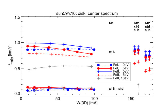
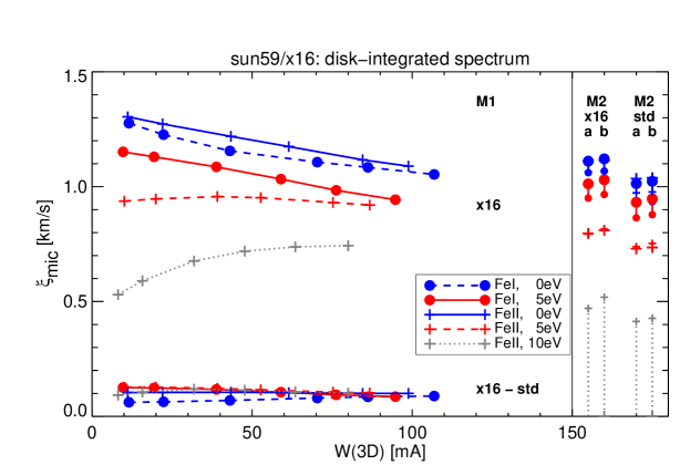
Figure 1 shows the determination of the microturbulence parameter from two different 3D model atmospheres of the Sun (see Tab. 1), according to methods M1 and M2. We considered $5$ sets of fictitious iron lines: Fe i with $E_{i}$=$0$ and $5$ eV, Fe ii with $E_{i}$=$0$, $5$, and $10$ eV. The $6$ lines of each set lie on a curve-of-growth with constant $E_{i}$, while $\log gf$ is varied to control the line strength such that it falls in the range $5$ mÅ $\la W_{\rm 3D}\la 100$ mÅ. We assume that all lines have the same wavelength, $\lambda=550$ nm.

3.1.1 Method 1

Obviously, the derived value of $\xi_{\rm mic}$ depends on the type and strength of the considered spectral line. M1 clearly reveals that high-excitation lines tend to ‘feel’ a lower microturbulence than low-excitation lines. At first sight, this is an unexpected result, because the high-excitation lines tend to form in the deeper photosphere where the velocity amplitudes are larger. At the same time, however, the vertical extent of the line forming region becomes narrower with increasing excitation potential, and thus the velocity variation probed by the spectral line decreases. Apparently, the latter effect dominates and leads to a reduced microturbulence broadening.

The dependence of $\xi_{\rm mic}$ on equivalent width $W$ is non-trivial. The results obtained from the evaluation of the disk-center spectrum indicate a rather weak dependence on line strength (Fig. 1, upper panel), while the disk-integrated spectrum exhibits a more pronounced $\xi_{\rm mic}$($W$) dependence, the slope of which is a function of excitation potential (Fig. 1, lower panel).

A very general result is that, for a given set of lines, the microturbulence derived from the disk-integrated (flux) spectra is systematically higher than that obtained from the disk-center (intensity) spectra, in agreement with observational evidence (e.g. Holweger et al., 1978). However, the ratio between $\xi_{\rm mic}$(flux) and $\xi_{\rm mic}$(intensity) depends again on the line properties, ranging from $\approx 1.5$ for weak low-excitation Fe i lines to $\la 1.1$ for weak high-excitation Fe ii lines.

Finally, we have to point out that the predicted microturbulence values depend slightly on the numerical resolution of the 3D model atmospheres used for the calculation of the synthetic line profiles. Increasing the spatial resolution by a factor of $2$ in the vertical direction, and by a factor $\sqrt{8}$ in each of the horizontal directions (decreasing $\Delta x$ =$\,\Delta y$ from $40$ to $14$ km, and $\Delta z$ from $15$ to $7.5$ km), leads to an increase of $\xi_{\rm mic}$ by roughly $0.1$ km/s for all type of lines. It remains unclear which numerical resolutions is needed to obtain fully converged microturbulence results. A minimum requirement is, of course, that the spacing of the hydrodynamical grid must be much smaller than the vertical extent of the line forming region.

Figure 3: Same as Fig. 1, but for one set of 15 real Fe i lines with $504$ nm $<\lambda<698$ nm, $1.5$ eV $<E_{i}<4.6$ eV (dots), and one set of 15 real Fe ii lines with $457$ nm $<\lambda<772$ nm, $2.8$ eV $<E_{i}<3.9$ eV (plus signs).

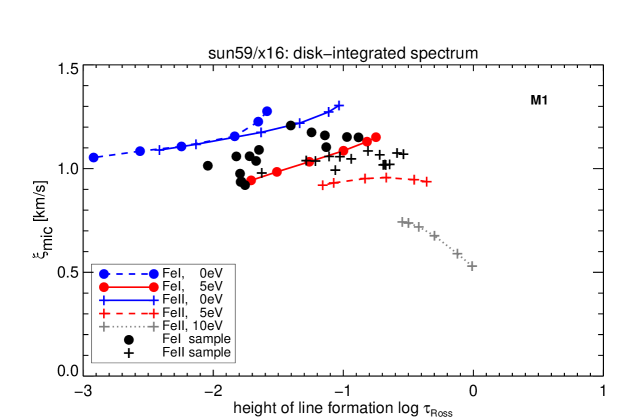
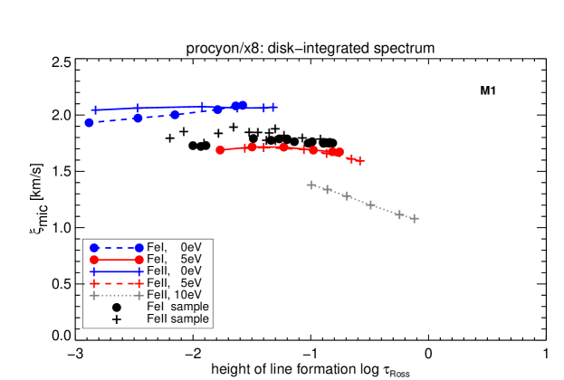
The fact that the derived microturbulence parameter depends on the considered ion, excitation potential, and line strength, shows that a constant microturbulence is not fully appropriate for representing the 3D hydrodynamical velocity field. In Fig. 2 we have plotted the microturbulence results (from disk-integrated spectra only) as a function of the line’s height of formation, to see whether the concept of a depth-dependent microturbulence might yield a more consistent picture. It is clear that $\xi_{\rm mic}$ is not simply a function of optical depth; it depends also on other properties of the line, in particular on the vertical extent of the line formation region. For this reason, a depth-dependent microturbulence model seems not very appealing.

Figure 4: Determination of the microturbulence parameter $\xi_{\rm mic}$ for two different Procyon models (t65g40mm00std and t65g40mm00x8b) from disk-integrated synthetic (flux) spectra according to methods M1, M2, and M3. Upper panel: $\xi_{\rm mic}$ obtained from $5$ sets of $6$ fictitious iron lines each (see legend) at $\lambda\,550$ nm. Lower panel: $\xi_{\rm mic}$ obtained from two sets of real lines ($18$ Fe i and $14$ Fe ii lines, respectively). The left part of each panel shows the results of M1, where $\xi_{\rm mic}$(t65g40mm00x8b) is shown together with the difference $\xi_{\rm mic}$(t65g40mm00x8b) - $\xi_{\rm mic}$(t65g40mm00std). The right part of the upper panel displays the results of M2 for both Procyon models, in the same representation as in Fig. 1 (smaller symbols: $\langle$3D$\rangle$, larger symbols: LHD). Similarly, the results obtained with M3 are shown in the right part of the lower panel.

Figure 5: Microturbulence parameter $\xi_{\rm mic}$ derived from high-resolution Procyon model t65g40mm00x8b according to method M1. The results are the same as shown in in Fig. 4, but are here plotted over the line’s height of formation (cf. Fig. 2).

3.1.2 Method 2

In general, M2a and M2b produce very similar results for a given 1D reference atmosphere (see Fig. 1, right sub-panels). This means that the ‘zero slope’ and the ‘minimum dispersion’ conditions are satisfied almost simultaneously, which is not surprising in the present case of a homogeneous sample of lines with identical $\lambda$ and $E_{i}$. However, we have no simple explanation for the fact that M2b always yields a slightly higher $\xi_{\rm mic}$ than M2a. For the 1D reference atmosphere, we have used the averaged 3D model, $\langle$3D$\rangle$, and the Holweger-Müller atmosphere (Holweger & Müller, 1974), HM. The difference $|\,$$\xi_{\rm mic}$($\langle$3D$\rangle$) - $\xi_{\rm mic}$(HM)$\,|$ derived with M2ab is significant but small ($\la 0.1$ km/s).

For Fe i, the microturbulence derived from M2 agrees closely with the minimum $\xi_{\rm mic}$ values obtained from M1 for the respective set of lines, i.e. with $\xi_{\rm mic}$ obtained from M1 for the stronger lines. This is also true for the low-excitation Fe ii lines ($E_{i}=0$ eV). However, M2 gives significantly lower values of $\xi_{\rm mic}$ than M1 for the high-excitation Fe ii lines. This is particularly clear for Fe ii, $E_{i}$=$10$ eV, at disk center: While M1 gives $\xi_{\rm mic}$ $\approx 0.55$ km/s, consistently for weak and strong lines, M2b gives $\xi_{\rm mic}$($\langle$3D$\rangle$) = $0.20$ km/s, and a negative $\xi_{\rm mic}$(HM); M2a fails to find a positive solution for $\xi_{\rm mic}$ with any of the 1D reference atmospheres. In other words, M2a requires a negative microturbulence in both of the 1D reference atmospheres to obtain a uniform abundance from the Fe ii, $E_{i}=10$ eV lines of different strength. This behavior is explained by deviations between the 1D and 3D thermal structures that lead to line strength dependent abundance corrections, which can only be compensated by a negative value of $\xi_{\rm mic}$. Note that this bias is not present in M1, which relies on a comparison of two models with identical thermal structure.

Adopting the microturbulence parameter obtained from Fe i lines of intermediate excitation potential ensures that the abundance derived from these lines will not depend systematically on line strength. With this choice of $\xi_{\rm mic}$, however, the high-excitation Fe ii lines will show a systematic line strength dependence, in the sense that stronger lines indicate lower abundances.

Finally, we note that M2 shows the same dependence on the numerical resolution of the 3D model atmospheres as M1.

3.1.3 Method 3

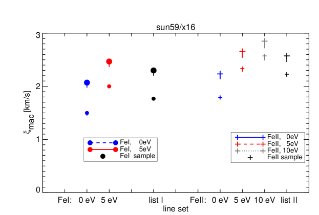
In addition to the fictitious lines discussed above, we have also employed two samples of real iron lines. Sample 1 comprises $15$ Fe i lines in the wavelength range $504$ nm $<\lambda<698$ nm, with excitation potential $1.5$ eV $<E_{i}<4.6$ eV, sample 2 consists of $15$ Fe ii lines with $457$ nm $<\lambda<772$ nm, $2.8$ eV $<E_{i}<3.9$ eV (see Caffau et al., 2011, Table. 2). As expected, the microturbulence determined from these lines with M1 fall within the results obtained from the fictitious lines (see Fig. 3). The wavelength dependence of $\xi_{\rm mic}$ is of minor importance in the considered wavelength range.

For both the Fe i and the Fe ii sample, the results of M3b and M1 are in reasonable agreement. Also, M3a and M3b give very similar answers in the case of the Fe ii sample. For the Fe i sample, however, M3a indicates a much lower $\xi_{\rm mic}$ value than M3b (see Fig. 3, right sub-panels). Obviously, M3a is more susceptible to the detailed properties of an inhomogeneous sample of spectral lines. In particular, the resulting $\xi_{\rm mic}$ can easily be biased by a correlation between excitation potential and line strength. For this reason, we prefer in general M3b over M3a.

Like M1 and M2, we find that also M3 indicates systematically higher $\xi_{\rm mic}$ values, by about $0.1$ km/s, for the high-resolution 3D model atmosphere of the Sun (sun59x16).

3.2 $\xi_{\rm mic}$ for Procyon

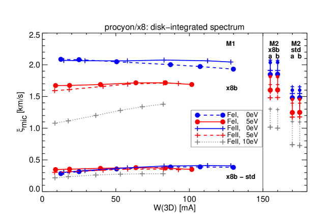
Figure 4 shows the determination of the microturbulence parameter from two different 3D model atmospheres representative of Procyon (t65g40mm00std and t65g40mm00x8b; see Tab. 1), according to methods M1, M2, and M3 applied to the disk-integrated synthetic flux spectra. We considered the same $5$ sets of fictitious iron lines as for the Sun, but with rescaled $\log gf$-values to adjust the line strengths such that they fall in the range between $5$ and $150$ mÅ ($\lambda=550$ nm).

  

Figure 6: Summary of macroturbulence determinations for the Sun (upper) and Procyon (lower) based on Method 1. Each symbol marks the average $\xi_{\rm mac}$ value obtained with the high-resolution 3D model from the same set of lines that was used for the derivation of $\xi_{\rm mic}$, as indicted in the legend and on the abscissa: two sets of fictitious and one sample of real Fe i lines (filled dots) and three sets of fictitious and one sample of real Fe ii lines (plus signs). Vertical lines connect each symbol to the corresponding result obtained with the standard (lower resolution) 3D model atmosphere. Smaller and larger symbols refer to disk-center and full-disk synthetic spectra, respectively.

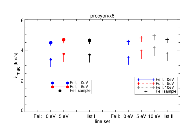
Method 1 shows a clear dependence of $\xi_{\rm mic}$ on excitation potential, in the sense that high-excitation lines indicate a significantly lower microturbulence than low-excitation lines. This is in agreement with the results obtained for the Sun, and seems to indicate that $\xi_{\rm mic}$ increases with height. At the same time, the microturbulence derived with M1 for given $E_{i}$ is essentially independent of line strength (except of the extreme case of the Fe ii lines with $E_{i}$=$10$ eV). This result appears to contradict the picture of a height-dependent microturbulence. Figure 5 illustrates the complex situation, which obviously cannot be described by a simple depth-dependence of $\xi_{\rm mic}$.

The results of method 2 are fully consistent with those of M1. This is not surprising in view of the fact that $\xi_{\rm mic}$ derived with M1 is almost independent of line strength for a given set of lines with constant $E_{i}$. As before, M2a and M2b agree closely. The choice of the 1D reference atmosphere has a significant influence on the resulting $\xi_{\rm mic}$: using the LHD model instead of the averaged $\langle$3D$\rangle$ model reduces the microturbulence by about $0.2$ km/s.

In the context of Method 3, we have used one sample of $18$ real Fe i lines in the wavelength range $506$ nm $<\lambda<562$ nm, with excitation potential $4.2$ eV $<E_{i}<4.5$ eV, and one sample of $14$ Fe ii lines with $449$ nm $<\lambda<646$ nm, $2.8$ eV $<E_{i}<3.9$ eV. These two sets of lines have only $2$ Fe ii lines in common with the samples of real iron lines used for the solar case. Since the range of $\lambda$ and $E_{i}$ is rather narrow, the microturbulence determined from these lines with M3 is consistent with the very uniform results obtained with M1 (see Fig. 4). M3a and M3b give essentially the same answer. Again, the $\xi_{\rm mic}$ values obtained with the LHD model are lower than those obtained with the $\langle$3D$\rangle$ model.

As for the solar case, we note that the predicted microturbulence values depend clearly on the numerical resolution of the 3D model atmospheres used for the calculation of the synthetic line profiles. Increasing the spatial resolution by a factor of $2$ in each of the three spatial directions, keeping everything else unchanged (t65g40mm00std $\rightarrow$ t65g40mm00x8a), leads to an increase of $\xi_{\rm mic}$ by roughly $0.2$ km/s for all type of lines. Reducing in addition the explicit turbulent viscosity in the hydrodynamical simulations by a factor $2$ (t65g40mm00x8a $\rightarrow$ t65g40mm00x8b) has a distinct impact as well, further increasing the spectroscopic microturbulence by $\approx$$0.15$ km/s. While it is clear that the ‘standard’ Procyon model (t65g40mm00std) underestimates $\xi_{\rm mic}$ significantly (more severely than the standard solar model underestimates the solar $\xi_{\rm mic}$) it remains unclear which microturbulence would be obtained in the limiting case of infinite numerical resolution.

Table 2: Empirical values of $\xi_{\rm mic}$ and $\xi_{\rm mac}$ from the literature, compared with the theoretical results derived in this work from different 3D CO5BOLD model atmospheres for the Sun and Procyon (average of results from Fe i, $E_{i}$ $=$  $0$ and $5$ eV, obtained with Method 2ab).

Atmosphere /	$\xi_{\rm mic}$ [km/s]		$\xi_{\rm mac}$ [km/s]		$v_{\rm turb}=\sqrt{(\xi_{\rm mic}^{2}+\xi_{\rm mac}^{2})/2}$  [km/s]
Model	disk-center	full-disk	disk-center	full-disk	disk-center	full-disk
Sun, observed${}^{\,a}$	$1.00\pm 0.15$	$1.35\pm 0.15$	$1.63\pm 0.15$	$1.90\pm 0.15$	$1.35\pm 0.10$	$1.65\pm 0.10$
3D solar models:
sun59std	$0.70\pm 0.05$	$0.95\pm 0.10$	$1.75\pm 0.25$	$2.20\pm 0.20$	$1.35\pm 0.20$	$1.70\pm 0.15$
sun59x16	$0.80\pm 0.05$	$1.05\pm 0.10$	$1.75\pm 0.25$	$2.30\pm 0.20$	$1.40\pm 0.20$	$1.80\pm 0.15$
Procyon, observed${}^{\,b}$	—	$2.10\pm 0.30$	—	$4.20\pm 0.50$	—	$3.30\pm 0.30$
3D Procyon models:
t65g40mm00std	$0.95\pm 0.15$	$1.40\pm 0.20$	$3.10\pm 0.25$	$4.40\pm 0.10$	$2.30\pm 0.20$	$3.30\pm 0.10$
t65g40mm00x8b	$1.45\pm 0.20$	$1.85\pm 0.25$	$3.60\pm 0.25$	$4.60\pm 0.10$	$2.75\pm 0.20$	$3.50\pm 0.10$

Notes: a: Holweger et al. (1978), full-disk values interpolated: $\xi^{2}$(full-disk)=$\xi^{2}$(disk-center)/2 + $\xi^{2}$(limb)/2;
b: Steffen (1985)

3.3 $\xi_{\rm mac}$ for the Sun and Procyon

We have derived the macroturbulence parameter $\xi_{\rm mac}$ from the 3D hydrodynamical model atmospheres using M1, as described in Sect. 2.2. The results for the Sun and Procyon are summarized in Fig. 6. Ignoring the Fe ii, $E_{i}$=$10$ eV lines, we find for the high-resolution solar model: $\xi_{\rm mac}$ = $1.9\pm 0.4$ km/s (disk-center) and $\xi_{\rm mac}$ = $2.4\pm 0.3$  km/s (integrated disk), respectively. The standard (lower resolution) solar model gives only slightly lower values. For Procyon, we find a macroturbulence that is roughly twice as large as for the Sun. The high-resolution model gives: $\xi_{\rm mac}$ = $3.7\pm 0.3$ km/s (disk-center) and $\xi_{\rm mac}$ = $4.7\pm 0.2$  km/s (integrated disk), respectively. The disk-center (integrated-disk) values are lower by $0.5$ km/s ($0.3$ km/s) when the standard 3D Procyon model with lower spatial resolution and higher viscosity is used to derive $\xi_{\rm mac}$.

3.4 Comparison with observation

In Table 2, we compare empirical micro- and macroturbulence determinations from the literature with the theoretical predictions of our hydrodynamical model atmospheres for the Sun and Procyon presented in this work. Somewhat arbitrarily, we consider here only the theoretical results obtained with Method 2ab from the fictitious Fe i lines.

The present investigation confirms the previous preliminary analysis by Steffen et al. (2009) (their Table 1), suggesting that the theoretical predictions of $\xi_{\rm mic}$ fall significantly below the classical empirical estimates, for both solar intensity and flux spectra, and even more clearly for Procyon. The high-resolution models (sun59x16 and t65g40mm00x8b) come closer to the empirical $\xi_{\rm mic}$ values, but still appear to be too low.

One has to keep in mind, however, that the empirical microturbulence was not determined in exactly the same way as in the theoretical approach. For a more reliable quantification of the low-$\xi_{\rm mic}$ problem, we shall derive the empirical microturbulence from observed spectra with Method 3, with exactly the same set of spectral lines (with well known $\log gf$ values) as adopted for the derivation of the theoretical $\xi_{\rm mic}$ values from the synthetic 3D spectra.

The macroturbulence values derived from the CO5BOLD models are somewhat larger than deduced from observations, such that the total non-thermal rms velocity $v_{\rm turb}$ (columns (6) and (7) of Tab. 2), and hence the total line broadening, appears to be very similar in simulations and observations. But even this quantity is not entirely independent of the numerical resolution of the 3D model atmospheres.

4 $\xi_{\rm mic}$ across the HRD

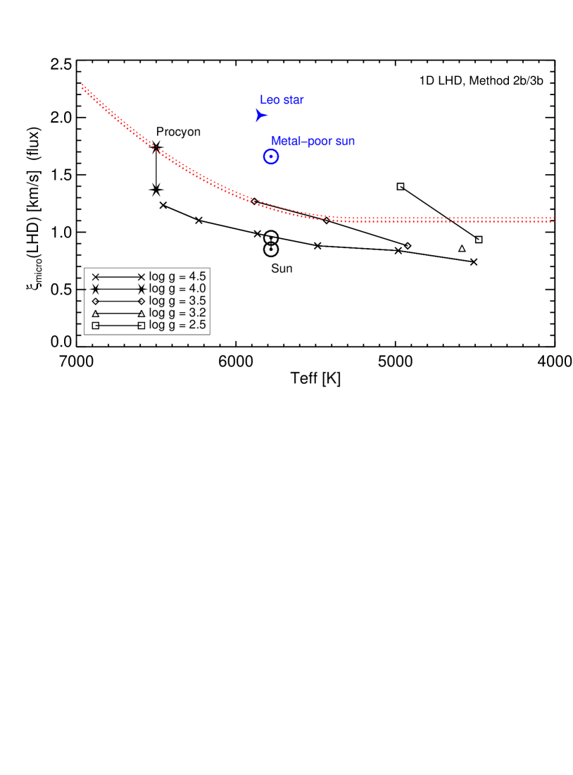
In addition to the Sun and Procyon, further 3D hydrodynamical model atmospheres, taken from the CIFIST 3D model atmosphere grid (Ludwig et al., 2009) and listed in Table 1, have been analyzed to get a first idea of how the predicted microturbulence varies across the Hertzsprung-Russell diagram. The results are given in Table 3 and Fig. 7. For the $12$ models representing the Main Sequence, Subgiants, and Giants, we have obtained $\xi_{\rm mic}$ from a list for $26$ real Fe i lines with $E_{i}>1.6$ eV, evaluated with M3b. For reference, we have added the Sun, Procyon, and the two metal-poor models from a different set of calculations, where we have instead used a set of $5$ fictitious Fe i lines with $E_{i}=3.0$ eV ($\lambda\,550$ nm) to derive $\xi_{\rm mic}$ according to M2b. In all cases, we have analyzed the disk-averaged flux spectra of the 3D model in comparison with two different 1D atmospheres, namely the LHD model with the same stellar parameters as the 3D model, and the average $\langle$3D$\rangle$ model.

Figure 7: Variation of the microturbulence parameter $\xi_{\rm mic}$ with $T\rm_{eff}$, $\log g$, and [M/H], as derived from the disk-integrated synthetic (flux) spectra of a number of 3D model atmospheres and the corresponding 1D LHD models (see Table 3 for more details). Different symbols indicate Main Sequence (crosses), Subgiants (diamonds), and Giants (squares). The two dotted curves represent an empirical microturbulence parameterization for main sequence stars (see text; lower and upper curve: $\log g$=4.5 and 4.0, respectively).

Table 3: Microturbulence derived from the disk-integrated (flux) spectra of a number of 3D model atmospheres probing a limited region of solar-like stars in the HRD.

3D Model	Meth.	$\xi_{\rm mic}$	$\alpha_{\rm MLT}$
		[km/s ]
Sun:
sun59std	M2b	0.85  (0.94)	0.5
sun59x16	M2b	0.95  (1.03)	0.5
Procyon:
t65g40mm00std	M2b	1.37  (1.53)	0.5
t65g40mm00x8b	M2b	1.74  (1.94)	0.5
Main sequence:
t45g45mm00n01	M3b	0.74  (0.48)	0.5
t50g45mm00n04	M3b	0.84  (0.65)	0.5
t55g45mm00n01	M3b	0.88  (0.80)	0.5
t59g45mm00n01	M3b	0.99  (0.97)	0.5
t63g45mm00n01	M3b	1.10  (1.14)	0.5
t65g45mm00n01	M3b	1.24  (1.26)	0.5
Subgiants:
t46g32mm00n01	M3b	0.86  (0.80)	0.5
t50g35mm00n01	M3b	0.88  (0.85)	0.5
t55g35mm00n01	M3b	1.10  (1.20)	0.5
t59g35mm00n01	M3b	1.27  (1.42)	0.5
Giants:
t45g25mm00n01	M3b	0.93  (0.93)	0.5
t50g25mm00n01	M3b	1.40  (1.51)	1.0
Metal-poor sun:
t57g44mm20n03	M2b	1.66  (0.82)	1.0
Leo star:
t59g40mm40n02	M2b	2.02  (0.98)	0.5

Notes: $\alpha_{\rm MLT}$ is the mixing length parameter used for the calculation of the 1D LHD reference model. Results obtained with Method 2b and 3b were obtained with a set of 5 fictitious Fe i lines ($E_{i}$=$3$ eV, $\lambda\,550$ nm) and a set of 26 real Fe i lines ($E_{i}>1.6$ eV), respectively. Numbers in parenthesis refer to the results obtained when replacing the LHD model with the $\langle$3D$\rangle$ model.

Figure 7 shows that the predicted $\xi_{\rm mic}$ increases systematically towards higher $T\rm_{eff}$ and lower $\log g$. This trend is in agreement with empirical evidence. However, we note that quantitatively the $\xi_{\rm mic}$ values predicted from the standard (low resolution, high viscosity) 3D model atmospheres are lower, by roughly $0.3$ km/s, than those obtained from the empirical relation recommended by the Gaia-ESO consortium. For main sequence and subgiants, this relation is given by

$$\xi_{\rm mic} = 1.15+2\,10^{-4}\,X+3.95\,10^{-7}\,X^{2}$$ (1)

$$- 0.13\,Y+0.13\,Y^{2}\quad\mathrm{[km/s]}\,,$$

with $X\equiv\max\{-250,T_{\rm eff}-5500\}$, $Y\equiv\log g-4$. It is indicated for $\log g$=4.5 and 4.0 by the (red) dotted lines in Fig. 7. The high-resolution Sun (sun59x16) lies clearly below this empirical relation, while the high-resolution Procyon model (t65g40mm00x8b) agrees closely.

Curiously, the two metal-poor models indicate an anomalously high microturbulence. This is, however, not a sign of increased turbulence in metal-poor stellar atmospheres. As evident from Table 3, this anomaly vanishes when doing the microturbulence determination with the $\langle$3D$\rangle$ model as the 1D reference. We conclude that the high microturbulence obtained with the LHD model is related to the fact that the temperature structures of LHD and $\langle$3D$\rangle$ model deviate strongly, in the sense that the $\langle$3D$\rangle$ model is much cooler in the upper photosphere. As a consequence, matching the 3D equivalent width of a low-excitation iron line with the LHD model requires a much higher iron abundance for strong lines than for weak lines, unless this mismatch is compensated by a high microturbulence. Observationally, this high-$\xi_{\rm mic}$ effect can probably not be verified due to the absence of sufficiently strong iron lines.

5 Discussion and conclusions

We have applied different methods to extract the parameters $\xi_{\rm mic}$ and $\xi_{\rm mac}$ from synthetic spectra based on 3D hydrodynamical atmospheres of a number of solar-type stars. We find that the different methods give consistent results. However, the derived turbulence parameters depend systematically on the properties of the selected spectral lines. It is thus not obvious how to assign a unique value of $\xi_{\rm mic}$ to a given stellar atmosphere.

For the Sun and Procyon, we have also demonstrated that the numerical viscosity and spatial resolution of the 3D model atmospheres still has a significant influence of the resulting micro- and macroturbulence, in the sense that the high-resolution models imply somewhat higher turbulence values. A preliminary comparison of the $\xi_{\rm mic}$ values predicted from the 3D simulations with the results of empirical studies found in the literature reveals that the theoretical predictions are systematically too low (see Table 2). The additional models included in the present study confirm this conclusion: a similar microturbulence discrepancy is seen for all solar-type main sequence stars (Fig. 7).

These findings suggests that the velocity field provided by the standard 3D hydrodynamical models is less ‘turbulent’ than it is in reality. While this conclusion seems to be in conflict with the claims by Asplund et al. (2000), it is confirmed by Allende Prieto et al. (2002), who find from their 3D Procyon model a systematic increase of the iron abundance with line strength, both for Fe i and Fe ii lines (see their Fig. 17). This translates to a microturbulence deficiency of about $0.3$ km/s, and implies a systematic overestimation of 3D abundances from stronger lines.

Our present results indicate that the discrepancy between theoretical and empirical $\xi_{\rm mic}$ is reduced, but not completely removed, when the latest 3D high-resolution model atmospheres are utilized. For a more reliable quantification of the remaining gap, we shall not rely on literature values of $\xi_{\rm mic}$, but instead intend to derive the empirical microturbulence from observed spectra with Method 3, in exactly the same way and with the same set of spectral lines (with well known $\log gf$ values) as adopted for the derivation of the theoretical $\xi_{\rm mic}$ values from the synthetic 3D spectra.

Further investigations are necessary to map the microturbulence problem across the Hertzsprung-Russell diagram, and to find an appropriate recipe to make the best use of the 3D models. A new generation of high-resolution, low viscosity 3D model atmospheres is certainly welcome in this respect. But it might still be necessary to introduce some (resolution-dependent) 3D microturbulence component in addition to the large-scale hydrodynamical velocity field of the 3D simulations, just for the purpose of an accurate representation of the non-thermal Doppler broadening of stronger spectral lines. Conceivably, the required small-scale velocity enhancement can be predicted by an appropriate turbulence model.

Appendix A Direct derivation of $\xi_{\rm mic}$ and $\xi_{\rm mac}$ from the hydrodynamical velocity field

A possible approach to deriving the disk-center ($\mu=1$) values of $\xi_{\rm mic}$ and $\xi_{\rm mac}$ directly from the 3D hydrodynamical velocity field is as follows:

First, a weighting function $w(\tau)$ is defined on a standard optical depth scale, e.g. $\tau=\tau_{\rm Ross}$, describing the contribution of the different photospheric layers to the formation of a typical line. Presumably, the weighting function is closely related to the line depression contribution function. It is normalized as

$$\int_{0}^{\infty}w(\tau)\;\mathrm{d}\tau=1\,.$$ (2)

Next, we compute the depth-weighted first and second moments of the vertical velocity $u_{z}$ at each horizontal position $(x,y)$ for all selected snapshots $t$:

$$\overline{u_{z}}(x,y,t)=\int_{0}^{\infty}u_{z}(x,y,\tau,t)\,w(\tau)\;\mathrm{d}\tau\,,$$ (3)

and

$$\overline{u_{z}^{2}}(x,y,t)=\int_{0}^{\infty}u_{z}^{2}(x,y,\tau,t)\,w(\tau)\;\mathrm{d}\tau\,.$$ (4)

The macroturbulence parameter is then computed as the variance of the local line shift $\overline{u_{z}}(x,y,t)$ over the stellar surface,

$$\xi_{\rm mac}^{2}=2\,\left(\,\left\langle\overline{u_{z}}^{2}(x,y,t)\right\rangle\,-\left\langle\overline{u_{z}}(x,y,t)\right\rangle^{2}\,\right)\,,$$ (5)

and the microturbulence parameter as the ($x,y,t$)-average of the local line-of-sight velocity dispersion,

$$\xi_{\rm mic}^{2}=2\,\left(\,\left\langle\overline{u_{z}^{2}}(x,y,t)\right\rangle\,-\left\langle\overline{u_{z}}^{2}(x,y,t)\right\rangle\,\right)\,,$$ (6)

where $\langle.\rangle$ denotes horizontal averaging over $(x,y)$ and temporal averaging over $t$. The total turbulent velocity is then

$$v_{\rm turb}^{2} = \left(\xi_{\rm mic}^{2}+\xi_{\rm mac}^{2}\right)/2$$ (7)

$$= \,\left\langle\overline{u_{z}^{2}}(x,y,t)\right\rangle\,-\left\langle\overline{u_{z}}(x,y,t)\right\rangle^{2}\,.$$

Taking into account the horizontal components of the hydrodynamical velocity field, $u_{x}$ and $u_{y}$, the procedure can be generalized to evaluate $\xi_{\rm mic}$ and $\xi_{\rm mac}$ values also for the disk-averaged spectrum:

$$\xi_{\rm mac}^{2} = \frac{1}{2}\,\left(\,\left\langle\overline{u_{x}}^{2}(x,y,t)\right\rangle\,-\left\langle\overline{u_{x}}(x,y,t)\right\rangle^{2}\,\right)$$ (8)

$$+ \frac{1}{2}\,\left(\,\left\langle\overline{u_{y}}^{2}(x,y,t)\right\rangle\,-\left\langle\overline{u_{y}}(x,y,t)\right\rangle^{2}\,\right)$$

$$+ \left(\,\left\langle\overline{u_{z}}^{2}(x,y,t)\right\rangle\,-\left\langle\overline{u_{z}}(x,y,t)\right\rangle^{2}\,\right)\,,$$

$$\xi_{\rm mic}^{2} = \frac{1}{2}\,\left(\,\left\langle\overline{u_{x}^{2}}(x,y,t)\right\rangle\,-\left\langle\overline{u_{x}}^{2}(x,y,t)\right\rangle\,\right)$$ (9)

$$+ \frac{1}{2}\,\left(\,\left\langle\overline{u_{y}^{2}}(x,y,t)\right\rangle\,-\left\langle\overline{u_{y}}^{2}(x,y,t)\right\rangle\,\right)$$

$$+ \left(\,\left\langle\overline{u_{z}^{2}}(x,y,t)\right\rangle\,-\left\langle\overline{u_{z}}^{2}(x,y,t)\right\rangle\,\right)\,,$$

$$v_{\rm turb}^{2} = \frac{1}{4}\,\left(\,\left\langle\overline{u_{x}^{2}}(x,y,t)\right\rangle\,-\left\langle\overline{u_{x}}(x,y,t)\right\rangle^{2}\,\right)$$ (10)

$$+ \frac{1}{4}\,\left(\,\left\langle\overline{u_{y}^{2}}(x,y,t)\right\rangle\,-\left\langle\overline{u_{y}}(x,y,t)\right\rangle^{2}\,\right)$$

$$+ \frac{1}{2}\,\left(\,\left\langle\overline{u_{z}^{2}}(x,y,t)\right\rangle\,-\left\langle\overline{u_{z}}(x,y,t)\right\rangle^{2}\,\right)\,.$$

First experiments have shown that the $\xi_{\rm mic}$ and $\xi_{\rm mac}$ values obtained with this method fall in the same range as those derived with the spectroscopic approach. However, the results depend sensitively on the choice of the weighting function $w$. Further thoughts are necessary to work out an appropriate definition of $w$. It might turn out that $w$ does not depend on optical depth only.