Electronic Raman scattering from orbital nematic fluctuations

Abstract

We compute Raman scattering intensities via the lowest-order coupling to the bosonic propagator associated with orbital nematic fluctuations in a minimal model for iron pnictides. The model consists of two bands on a square lattice exhibiting four Fermi pockets and a transition from the normal to a nematic state. It is shown that the orbital fluctuations produce in the $B_{1g}$ channel strong quasi-elastic light scattering around the nematic critical temperature $T_{n}$, both above and below $T_{n}$. This holds for the $A_{1g}$ symmetry only below $T_{n}$ whereas no low-energy scattering from orbital fluctuations is found in the $B_{2g}$ symmetry. Due to the nematic distortion the electron pocket at the $X$-point may disappear at low temperatures. Such a Lifshitz transition causes in the $B_{2g}$ spectrum a large upward shift of spectral weight in the high energy region whereas no effect is seen in the other symmetries.

I Introduction

Electronic nematic states are electronic analogues of nematic liquid crystals, which break only the orientational symmetry, but retain the other symmetries of the system. Electronic nematicity is discussed in a number of correlated electron systems such as quantum spin systems, K. Penc and A. M. Läuchli (2011) two-dimensional electron gases, M. P. Lilly, K. B. Cooper, J. P. Eisenstein, L. N. Pfeiffer, and K. W. West (1999); R. R. Du, D. C. Tsui, H. L. Stormer, L. N. Pfeiffer, K. W. Baldwin, K. W. West (1999) cuprate superconductors, Kivelson et al. (2003); M. Vojta (2009) bilayer ruthenates, A. P. Mackenzie, J. A. N. Bruin, R. A. Borzi, A. W. Rost, and S. A. Grigera (2012) and iron pnictides. I. R. Fisher, L. Degiorgi, and Z. X. Shen (2011) Depending on electronic degrees of freedom responsible for nematic order, we may distinguish between three kinds of nematicity. i) The charge nematicity which is obtained either by partial melting of charge stripes Kivelson et al. (1998) or by a Pomeranchuk instability, yam ; Halboth and Metzner (2000) ii) the spin nematicity which is driven by frustration between magnetic interactions, A. F. Andreev and I. A. Grishchuk (1984) and iii) the orbital nematicity due to orbital order caused, for example, by a spontaneous occupation difference between $d_{yz}$ and $d_{zx}$ orbitals in $d$-electron systems. S. Raghu, A. Paramekanti, E-.A. Kim, R. A. Borzi, S. A. Grigera, A. P. Mackenzie, and S. A. Kivelson (2009); W.-C. Lee and C. Wu (2009)

In iron pnictides, electronic nematicity is associated with the tetragonal-orthorhombic structural phase transition. I. R. Fisher, L. Degiorgi, and Z. X. Shen (2011) The structural transition is believed to be driven primarily by coupling to the electronic system. In fact, electronic resistivity exhibits a pronounced anisotropy by applying a uniaxial strain to the system. Moreover, angle-resolved photoemission spectroscopy I. R. Fisher, L. Degiorgi, and Z. X. Shen (2011); Y. Zhang, C. He, Z. R. Ye, J. Jiang, F. Chen, M. Xu, Q. Q. Ge, B. P. Xie, J. Wei, M. Aeschlimann, X. Y. Cui, M. Shi, J. P. Hu, and D. L. Feng (2011) revealed directly a sizable energy difference of $d_{yz}$ and $d_{zx}$ orbitals, indicating the importance of orbital nematicity. F. Krüger, S. Kumar, J. Zaanen, and J. van den Brink (2009); C.-C. Lee, W.-G. Yin, and W. Ku (2009); W. Lv, J. Wu, and P. Phillips (2009); Y. Yanagi, Y. Yamakawa, N. Adachi, and Y. Ōno (2010); H. Kontani, T. Saito, and S. Onari (2011) Since the structural transition occurs slightly above a spin-density-wave (SDW) phase, spin nematicity is also discussed as a plausible scenario C. Fang, H. Yao, W.-F. Tsai, J. Hu, and S. A. Kivelson (2008); C. Xu, Y. Qi, and S. Sachdev (2008); R. Fernandes and J. Schmalian (2012).

Quite recently a nematic instability was observed also in magnetic torque measurements, S. Kasahara, H. J. Shi, K. Hashimoto, S. Tonegawa, Y. Mizukami, T. Shibauchi, K. Sugimoto, T. Fukuda, T. Terashima, A. H. Nevidomskyy, and Y. Matsuda (2012) which are very sensitive to the breaking of a fourfold symmetry. The observed critical temperature is much higher than the onset temperature of the SDW phase and extends to regions far away from the SDW phase. It seems therefore reasonable to associate such a nematic instability to orbital nematicity. S. Kasahara, H. J. Shi, K. Hashimoto, S. Tonegawa, Y. Mizukami, T. Shibauchi, K. Sugimoto, T. Fukuda, T. Terashima, A. H. Nevidomskyy, and Y. Matsuda (2012)

Measurements of the anisotropy of the resistivity and magnetic torque provide only indirect evidence of electronic nematicity. In the case of charge nematicity, it was shown theoretically Yamase and Zeyher (2011) that the Raman spectroscopy in the $B_{1g}$ channel in a tetragonal system measures directly the charge nematic correlation function. Since the nematic instability does not break translational symmetry and thus is characterized by momentum zero, it is natural to believe that the Raman spectroscopy can become a suitable method to detect also orbital nematicity.

In the present paper, we provide a microscopic understanding of Raman scattering by orbital nematic fluctuations. In Sec. 2 we introduce a minimal two-band model for iron pnictides, which exhibits an orbital nematic instability at low temperatures and four Fermi pockets. The Raman scattering intensity is then computed in the lowest-order of the bosonic propagator associated with nematic fluctuations. Numerical results both in the normal and nematic states and their interpretation are presented in Sec. 3. The effect of Coulomb screening is also studied. Our conclusions then follow in Sec. 4.

II model and formalism

II.1 Nematic transition in a minimal two-band model

Our model Hamiltonian has the form $H=H_{0}+H_{1}$ where the interaction part $H_{1}$ is given by

$$H_{1}=\frac{g}{2}\sum_{i}n_{i-}n_{i-}.$$ (1)

The difference density operator $n_{i-}$ is defined by $n_{i-}=n_{i1}-n_{i2}$ with the density operator $n_{i\alpha}=\sum_{\sigma}c^{\dagger}_{i\alpha\sigma}c_{i\alpha\sigma}$. $i$ and $\sigma$ are site and spin indices, respectively, and $\alpha=1,2$ is a band index. $g$ is a coupling constant which is considered as a parameter in our model. An expression for $H_{0}$ suitable for pnictides is S. Raghu, X.-L. Qi, C.-X. Liu, D. J. Scalapino, and S.-C. Zhang (2008); Zi-Jian Yao, Jian-Xin Li, and Z. D Wang (2009)

$$H_{0}=\sum_{{\bf k},\sigma,\alpha,\beta}\epsilon^{\alpha\beta}_{\bf k}c^{\dagger}_{{\bf k}\alpha\sigma}c_{{\bf k}\beta\sigma},$$ (2)

with

$$\epsilon^{11}_{\bf k}=-2t_{1}\cos k_{x}-2t_{2}\cos k_{y}-4t_{3}\cos k_{x}\cos k_{y},$$ (3)

$$\epsilon^{22}_{\bf k}=-2t_{2}\cos k_{x}-2t_{1}\cos k_{y}-4t_{3}\cos k_{x}\cos k_{y},$$ (4)

$$\epsilon^{12}_{\bf k}=-4t_{4}\sin k_{x}\sin k_{y}.$$ (5)

Reasonable values for the hopping amplitudes are Zi-Jian Yao, Jian-Xin Li, and Z. D Wang (2009) $t=-t_{1},t_{2}/t=1.5,t_{3}/t=-1.2,t_{4}/t=-0.95$, which we will also use in our calculations. The band indices $\alpha=1$ and $2$ originate mainly from the $d_{zx}$ and $d_{yz}$ orbitals, respectively. In the following energies are always given in units of $t$.

Taking $H_{1}$ into account the Green’s function matrix in band space is given in mean-field approximation by

$$\hat{G}({\bf k},\omega)={\begin{pmatrix}\omega+i\delta-\xi_{{\bf k}1}&-\epsilon^{12}_{\bf k}\\ -\epsilon^{12}_{\bf k}&\omega+i\delta-\xi_{{\bf k}2}\end{pmatrix}}^{-1}$$ (6)

with

$$\xi_{{\bf k}1}=\epsilon^{11}_{\bf k}-\mu+gn_{-},$$ (7)

$$\xi_{{\bf k}2}=\epsilon^{22}_{\bf k}-\mu-gn_{-},$$ (8)

and $n_{-}=\langle n_{i-}\rangle$. $\langle...\rangle$ denotes the expectation value, $\mu$ is the chemical potential, and $\delta$ an infinitesimally small positive quantity. Carrying out the inversion in Eq. (6), rearranging terms and using Pauli matrixes $\hat{\tau}_{1},\hat{\tau}_{2},\hat{\tau}_{3}$ as well as the $2\times 2$ unit matrix $\hat{\tau}_{0}$ we find

$$\hat{G}({\bf k},\omega)=g_{0}\hat{\tau}_{0}+g_{1}\hat{\tau}_{1}+g_{2}\hat{\tau}_{3},$$ (9)

$$g_{0}=\frac{1}{2}\left(\frac{1}{\omega-\lambda^{+}_{\bf k}+i\delta}+\frac{1}{\omega-\lambda^{-}_{\bf k}+i\delta}\right),$$ (10)

$$g_{1}=\frac{1}{2}\frac{\epsilon^{12}_{\bf k}}{E_{\bf k}}\left(\frac{1}{\omega-\lambda^{+}_{\bf k}+i\delta}-\frac{1}{\omega-\lambda^{-}_{\bf k}+i\delta}\right),$$ (11)

$$g_{3}=\frac{1}{2}\frac{\xi^{-}_{\bf k}}{E_{\bf k}}\left(\frac{1}{\omega-\lambda^{+}_{\bf k}+i\delta}-\frac{1}{\omega-\lambda^{-}_{\bf k}+i\delta}\right).$$ (12)

Here we used the abbreviations

$$\lambda^{\pm}_{\bf k}=\xi^{+}_{\bf k}\pm E_{\bf k},$$ (13)

$$\xi^{\pm}_{\bf k}=\frac{1}{2}(\xi_{{\bf k}1}\pm\xi_{{\bf k}2}),$$ (14)

$$E_{\bf k}=\sqrt{(\xi^{-}_{\bf k})^{2}+(\epsilon^{12}_{\bf k})^{2}}.$$ (15)

$n_{-}$ satisfies the following nonlinear equation,

$$n_{-}=\frac{2}{N}\sum_{\bf k}\frac{\xi^{-}_{\bf k}}{E_{\bf k}}\left[f(\lambda^{+}_{\bf k})-f(\lambda^{-}_{\bf k})\right].$$ (16)

Figure 1: (Color online) Dispersion of the two bands along symmetry directions in the normal (upper panel) and nematic (middle panel) state. The Fermi energy corresponds to zero. The bottom panel shows the nematic order parameter $n_{-}$ as a function of temperature $T$. Left and right insets depict the Fermi lines in the nematic state at low temperatures and in the normal state, respectively.

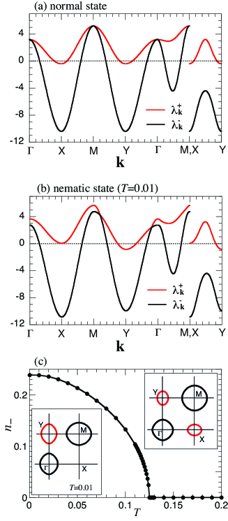
The dispersion of the two bands in the normal state is shown in the upper panel in Fig. 1. The special $\bf k$-points are $\Gamma=(0,0)$, $X=(\pi,0)$, $M=(\pi,\pi)$, and $Y=(0,\pi)$, and the dispersion is drawn along the lines passing through these points. The band $\lambda^{+}_{{\bf k}}(\lambda^{-}_{{\bf k}})$ crosses the Fermi energy around $X$ and $Y$ ($\Gamma$ and $M$) points. Consequently, the Fermi lines form two electron pockets at $X$ and $Y$ and two hole pockets at $\Gamma$ and $M$, as shown in the right inset of the bottom panel. At lower temperature our model exhibits for negative values of $g$ a nematic phase transition, i.e., a line which separates states where $n_{-}$ is zero from those where it is nonzero. The solid line in Fig. 1(c) depicts the temperature dependence of the order parameter $n_{-}$. In the nematic phase, where $n_{-}\neq 0$, the point group is reduced from $C_{4v}$ to $C_{2v}$. As a result the pockets at the $X$ and $Y$ points are no longer related by symmetry. The electron pocket at the $X$ point shrinks while that at the $Y$ point expands. When $n_{-}$ becomes sufficiently large a Lifshitz transition can occur at low temperatures where the pocket at the $X$ point vanishes. This is illustrated in Fig. 1(b) and in the left inset of Fig. 1(c).

II.2 Raman scattering intensity

The Raman scattering intensity $S^{\gamma}(\omega)$ is given by

$$S^{\gamma}(\omega)=-\frac{1}{\pi}[1+b(\omega)]{\rm Im}\chi^{\gamma}(\omega)\,,$$ (17)

where $b(\omega)$ is the Bose function $(e^{\beta\omega}-1)^{-1}$ and $\beta^{-1}=T$ the temperature. $\chi^{\gamma}(\omega)$ is the retarded Green’s function

$$\chi^{\gamma}(\omega)=-\frac{i}{N}\int_{0}^{\infty}dte^{i(\omega+i{\delta})t}\langle[\rho^{\gamma}(t),\rho^{\gamma}(0)]\rangle,$$ (18)

where $N$ is the number of lattice sites, $[\cdot,\cdot]$ the commutator, and $\rho^{\gamma}(t)$ the operator

$$\rho^{\gamma}=\sum_{{\bf k},\sigma,\alpha,\beta}\gamma_{\alpha\beta}({\bf k})c^{\dagger}_{{\bf k}\alpha\sigma}c_{{\bf k}\beta\sigma}$$ (19)

in the Heisenberg picture. $\gamma_{\alpha\beta}({\bf k})$ is the Raman vertex in the effective mass approximation given by

$$\gamma_{\alpha\beta}({\bf k})=\sum_{r,s}e_{r}^{i}\frac{\partial^{2}\epsilon^{\alpha\beta}_{\bf k}}{\partial k_{r}\partial k_{s}}e^{f}_{s}.$$ (20)

${\bf e}^{i}$ and ${\bf e}^{f}$ are the polarization vectors of the incident and scattered light, respectively.

The underlying point group $C_{4v}$ gives rise to three independent cross sections corresponding to the representations $B_{1g},B_{2g}$, and $A_{1g}$. The $B_{1g}$ contribution is obtained by taking the polarization vectors ${\bf e}^{i}=\frac{1}{\sqrt{2}}(1,1)$ and ${\bf e}^{f}=\frac{1}{\sqrt{2}}(1,-1)$ which yields

$$\gamma_{\alpha\beta}^{B_{1g}}({\bf k})=\frac{1}{2}\left(\frac{\partial^{2}\epsilon^{\alpha\beta}_{\bf k}}{\partial k_{x}^{2}}-\frac{\partial^{2}\epsilon^{\alpha\beta}_{\bf k}}{\partial k_{y}^{2}}\right).$$ (21)

It is convenient to consider $\gamma^{B_{1g}}_{\alpha\beta}$ as a matrix in band space $\hat{\gamma}^{B_{1g}}$ and to express the dependence on $\alpha$ and $\beta$ in terms of Pauli matrices $\hat{\tau}_{1},\hat{\tau}_{2},\hat{\tau}_{3}$. Inserting the explicit expressions for $\epsilon^{\alpha\beta}_{\bf k}$ we obtain

$$\hat{\gamma}^{B_{1g}}={\gamma}^{B_{1g}}_{0}\hat{\tau}_{0}+{\gamma}^{B_{1g}}_{3}\hat{\tau}_{3},$$ (22)

with

$${\gamma}^{B_{1g}}_{0}=\frac{t_{1}+t_{2}}{2}(\cos k_{x}-\cos k_{y}),$$ (23)

$${\gamma}^{B_{1g}}_{3}=\frac{t_{1}-t_{2}}{2}(\cos k_{x}+\cos k_{y}).$$ (24)

In a similar way the $B_{2g}$ contribution to the Raman vertex is obtained by taking ${\bf e}^{i}=(1,0)$ and ${\bf e}^{f}=(0,1)$:

$$\hat{\gamma}^{B_{2g}}={\gamma}^{B_{2g}}_{0}\hat{\tau}_{0}+{\gamma}^{B_{2g}}_{1}\hat{\tau}_{1},$$ (25)

$${\gamma}^{B_{2g}}_{0}=-4t_{3}\sin k_{x}\sin k_{y},$$ (26)

$${\gamma}^{B_{2g}}_{1}=-4t_{4}\cos k_{x}\cos k_{y}.$$ (27)

For the polarization vectors ${\bf e}^{i}={\bf e}^{f}=\frac{1}{\sqrt{2}}(1,1)$, both $A_{1g}$ and $B_{2g}$ channels contribute to the Raman intensity. Subtracting the latter the $A_{1g}$ contribution becomes

$$\hat{\gamma}^{A_{1g}}={\gamma}^{A_{1g}}_{0}\hat{\tau}_{0}+{\gamma}^{A_{1g}}_{1}\hat{\tau}_{1}+{\gamma}^{A_{1g}}_{3}\hat{\tau}_{3},$$ (28)

$${\gamma}^{A_{1g}}_{0}=\frac{t_{1}+t_{2}}{2}(\cos k_{x}+\cos k_{y})+4t_{3}\cos k_{x}\cos k_{y},$$ (29)

$${\gamma}^{A_{1g}}_{1}=4t_{4}\sin k_{x}\sin k_{y},$$ (30)

$${\gamma}^{A_{1g}}_{3}=\frac{t_{1}-t_{2}}{2}(\cos k_{x}-\cos k_{y}).$$ (31)

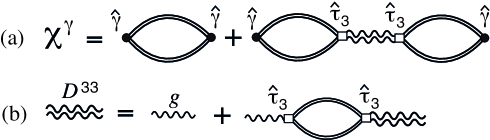
Using the random phase approximation $\chi^{\gamma}(\omega)$ is given by the bubble diagrams depicted in Fig. 2. The label $\hat{\gamma}$ stands for one of the three Raman vertices $\hat{\gamma}^{B_{1g}}$, $\hat{\gamma}^{B_{2g}}$ or $\hat{\gamma}^{A_{1g}}$. The vertex $\hat{\tau_{3}}$ originates from the interaction $H_{1}$. The solid and wavy lines denote the electron Green’s function and the interaction $g$, respectively. The double wavy line represents the propagator $D^{33}$ for orbital fluctuations. Figures 2(a) and 2(b) are equivalent to the following equations,

$$\chi^{\gamma}(\omega)=\Pi^{\gamma\gamma}(\omega)+\Pi^{\gamma 3}(\omega)D^{33}(\omega)\Pi^{3\gamma}(\omega),$$ (32)

$$D^{33}(\omega)=\frac{g}{1-g\Pi^{33}(\omega)}.$$ (33)

Here $\Pi^{\gamma 3}$ ($\Pi^{33}$) denotes a bare bubble with the vertices $\hat{\gamma}$ and $\hat{\tau_{3}}$ ($\hat{\tau_{3}}$ and $\hat{\tau_{3}}$).

Figure 2: Diagrams for the Raman susceptibility $\chi^{\gamma}$ and the propagator $D^{33}$ for orbital fluctuations. $\hat{\gamma}$ denotes Raman vertices and $\hat{\tau_{3}}$ a vertex coming from the interaction $H_{1}$.

Let us calculate $\Pi^{\alpha\gamma}(\omega)$ for general vertices

$$\hat{\alpha}_{\bf k}=\alpha_{0}\hat{\tau}_{0}+\alpha_{1}\hat{\tau}_{1}+\alpha_{3}\hat{\tau}_{3},$$ (34)

$$\hat{\gamma}_{\bf k}=\gamma_{0}\hat{\tau}_{0}+\gamma_{1}\hat{\tau}_{1}+\gamma_{3}\hat{\tau}_{3}\,.$$ (35)

Performing the internal frequency sum by means of the spectral function

$$\hat{A}({\bf k},\omega)=-\frac{1}{\pi}{\rm Im}\hat{G}({\bf k},\omega),$$ (36)

and carrying out an analytic continuation we obtain for the imaginary part of $\Pi^{\alpha\gamma}(\omega)$,

$${\rm Im}\Pi^{\alpha\gamma}(\omega)=\frac{2\pi}{N}\sum_{\bf k}\int d\epsilon{\rm Tr}\left[\hat{\alpha}_{\bf k}\hat{A}({\bf k},\epsilon)\hat{\gamma}_{\bf k}\hat{A}({\bf k},\epsilon+\omega)\right]\left[f(\epsilon+\omega)-f(\epsilon)\right],$$ (37)

where $f$ is the Fermi function. Writing

$$\hat{A}({\bf k},\omega)=A_{0}\hat{\tau}_{0}+A_{1}\hat{\tau}_{1}+A_{3}\hat{\tau}_{3},$$ (38)

we obtain from Eqs. (9)-(12) the following expressions for the coefficients,

$$A_{0}=\frac{1}{2\pi}\left[\frac{\delta}{(\omega-\lambda_{\bf k}^{+})^{2}+\delta^{2}}+\frac{\delta}{(\omega-\lambda_{\bf k}^{-})^{2}+\delta^{2}}\right],$$ (39)

$$A_{1}=\frac{1}{2\pi}\frac{\epsilon_{\bf k}^{12}}{E_{\bf k}}\left[\frac{\delta}{(\omega-\lambda_{\bf k}^{+})^{2}+\delta^{2}}-\frac{\delta}{(\omega-\lambda_{\bf k}^{-})^{2}+\delta^{2}}\right],$$ (40)

$$A_{3}=\frac{1}{2\pi}\frac{\xi^{-}_{\bf k}}{E_{\bf k}}\left[\frac{\delta}{(\omega-\lambda_{\bf k}^{+})^{2}+\delta^{2}}-\frac{\delta}{(\omega-\lambda_{\bf k}^{-})^{2}+\delta^{2}}\right].$$ (41)

Carrying out the ${\rm Tr}$ in Eq. (37) the imaginary part of the considered bubble can be written as

$${\rm Im}\Pi^{\alpha\gamma}(\omega)=\frac{4\pi}{N}\sum_{\bf k}\int d\epsilon({\bf G}^{\alpha}\cdot{\bf G}^{\gamma\prime})\left[f(\epsilon+\omega)-f(\epsilon)\right],$$ (42)

where the scalar product of two four-dimensional vectors ${\bf G}^{\alpha}$ and ${\bf G}^{\gamma\prime}$ appears. The components of these vectors are given by

$$G^{\alpha}_{0}=\alpha_{0}A_{0}+\alpha_{1}A_{1}+\alpha_{3}A_{3},$$ (43)

$$G^{\alpha}_{1}=\alpha_{0}A_{1}+\alpha_{1}A_{0},$$ (44)

$$G^{\alpha}_{2}=-i\alpha_{1}A_{3}+i\alpha_{3}A_{1},$$ (45)

$$G^{\alpha}_{3}=\alpha_{0}A_{3}+\alpha_{3}A_{0},$$ (46)

and

$$G^{\gamma\prime}_{0}=\gamma_{0}A_{0}^{\prime}+\gamma_{1}A_{1}^{\prime}+\gamma_{3}A_{3}^{\prime},$$ (47)

$$G^{\gamma\prime}_{1}=\gamma_{0}A_{1}^{\prime}+\gamma_{1}A_{0}^{\prime},$$ (48)

$$G^{\gamma\prime}_{2}=-i\gamma_{1}A_{3}^{\prime}+i\gamma_{3}A_{1}^{\prime},$$ (49)

$$G^{\gamma\prime}_{3}=\gamma_{0}A_{3}^{\prime}+\gamma_{3}A_{0}^{\prime}.$$ (50)

$A_{i}^{\prime}({\bf k},\omega)$ is defined by $A_{i}({\bf k},\omega+\epsilon)$. All the susceptibilities $\Pi$ occurring in Eqs. (32) and (33) can be obtained from the general expression Eq. (42) as special cases. Explicit expressions are given in the appendix. The calculation of the various susceptibilities in the Raman scattering intensity $S^{\gamma}(\omega)$ [Eq. (17)] has thus been reduced to one frequency and one two-dimensional momentum integration which have to be carried out numerically. The corresponding real parts can be obtained by a Kramers-Kronig transformation.

III Results

We first present a general symmetry argument which shows that orbital nematic fluctuations couple in the normal state only to the $B_{1g}$ channel and in the nematic state to both $B_{1g}$ and $A_{1g}$ channels. We then present numerical results for the Raman spectra by computing the diagrams shown in Fig. 2. The most interesting effect due to orbital nematic fluctuations is the appearance of a central mode in some of the Raman spectra. We will show that its main properties can be understood from analytic considerations. We will also study the effect of Coulomb screening on our obtained results.

III.1 Selection rules

As seen in Fig. 2(a), orbital nematic fluctuations couple to the Raman susceptibility via a bubble diagram with vertices $\hat{\gamma}$ and $\hat{\tau}_{3}$. This diagram determines our selection rules for nematic fluctuations.

In the normal state the symmetry group of our system is $C_{4v}$. To see how the band basis transforms under its group elements, we consider each term on the right-hand side of Eq. (28). In the first term it is clear that both $\gamma_{0}^{A_{1g}}$ and $\hat{\tau}_{0}$ have $A_{1g}$ symmetry. In the second term $\gamma_{1}^{A_{1g}}$ has $B_{2g}$ symmetry whereas the product of $\gamma_{1}^{A_{1g}}$ and $\hat{\tau}_{1}$ should transform as $A_{1g}$, which means that $\hat{\tau}_{1}$ has $B_{2g}$ symmetry. In the third term, $\gamma_{3}^{A_{1g}}$ has $B_{1g}$ symmetry and thus $\hat{\tau}_{3}$ should also have $B_{1g}$ symmetry so that their product transforms as $A_{1g}$. Since $\hat{\tau}_{3}$ has $B_{1g}$ symmetry, the bubble with vertices $\hat{\gamma}$ and $\hat{\tau}_{3}$ is finite for $\hat{\gamma}^{B_{1g}}$ and vanishes otherwise. This leads to our selection rule that orbital nematic fluctuations can be observed in the normal state only in the $B_{1g}$ channel.

In the nematic phase the point group is reduced to $C_{2v}$. $A_{1g}$ and $B_{1g}$ denote then the same representation. Hence not only the bubble with $\hat{\gamma}^{B_{1g}}$ and $\hat{\tau}_{3}$ but also that with $\hat{\gamma}^{A_{1g}}$ and $\hat{\tau}_{3}$ can be nonzero. That is, in the nematic state orbital nematic fluctuations can be observed in both $B_{1g}$ and $A_{1g}$ channels but not in the $B_{2g}$ channel.

The obtained selection rules can also be verified by computing $\Pi^{\gamma 3}(\omega)$ directly. In the Appendix we indeed find in this way that $\Pi^{A_{1g}3}$ is zero in the normal state and that $\Pi^{B_{2g}3}$ is zero both in the normal and nematic states.

III.2 Raman spectra

We compute numerically the Raman susceptibilities Eq. (32) [see also Fig. 2] using the chemical potential $\mu=0.6$ and the coupling strength $g=-1.907$ as representative values. They lie in a region of the phase diagram where the normal state at high temperatures transforms at a transition temperature $T_{n}=0.125$ into a homogenous nematic state at low temperatures [see Fig. 1(c)]. In the following calculations we choose finite values for $\delta$ instead of taking the limit $\delta\rightarrow 0$ in Eqs. (10)-(12) and (39)-(41). This means that we replace $\delta$-functions in the spectral function by Lorentzians with width $\delta$, which corresponds to the introduction of a phenomenological self-energy. Such a procedure is necessary because intraband contributions to the Raman scattering intensity can be taken properly into account only in the presence of self-energies. We have obtained qualitatively the same results for $\delta=0.05$, $0.1$, and $0.2$, and thus will present only the results for $\delta=0.1$.

III.2.1 B_1g Raman scattering

Figure 3: (Color online) Panel (a) and (c): Im$\chi^{B_{1g}}(\omega)$ for temperatures below and above $T_{n}$, respectively. Panel (b) and (d): $S^{B_{1g}}(\omega)$ for the same temperatures.

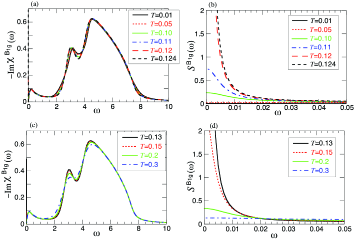
The left panels in Fig. 3 show Im$\chi^{B_{1g}}(\omega)$ for various temperatures below and above the transition temperature $T_{n}$, respectively, over a large energy interval of the order of the band width. In such a representation no distinct temperature dependence is visible even if the system enters the nematic phase. According to Eq. (32) the Raman susceptibility $\chi^{B_{1g}}$ consists of two terms. The first one is the bare susceptibility $\Pi^{B_{1g}{B_{1g}}}$ which is rather independent of temperature and dominates in the energy interval of the figures. The main peak at about $4.5t$ arises from interband transitions near the points $(\pi/4,\pi/4)$ and $(3\pi/4,3\pi/4)$ in agreement with the band structure shown in Figs. 1(a) and 1(b). The effect of the second term in Eq. (32) is only moderate and generates a second peak at about $3t$. This means that in a good approximation the curves in the left panels of Fig. 3 represent at temperatures well below or above $T_{n}$ the first term in Eq. (32).

The second term in Eq. (32), however, plays a very important role near $T_{n}$ where orbital nematic fluctuations substantially develop and become critical. As a result a central peak emerges in a very small frequency interval around $\omega=0$. In the right panels of Fig. 3 we plot the scattering intensity $S^{B_{1g}}(\omega)$ [Eq. (17)], not the imaginary part of the Raman susceptibility, to depict the spectrum in the very low energy region. We see that with decreasing temperature a central peak starts to develop below $T=0.3$, with a peak height at $\omega=0$ which diverges at $T=T_{n}$. Entering the nematic phase the central peak is suppressed and completely vanishes below $T\approx 0.05$. For temperatures far away from $T_{n}$ the total intensity is given approximately by the first term in Eq. (32) and is small and practically constant at very low energies.

III.2.2 A_1g Raman scattering

Figure 4: (Color online) Panel (a) and (c): Im$\chi^{A_{1g}}(\omega)$ for temperatures below and above $T_{n}$, respectively. Panel (b) and (d): $S^{A_{1g}}(\omega)$ for the same temperatures.

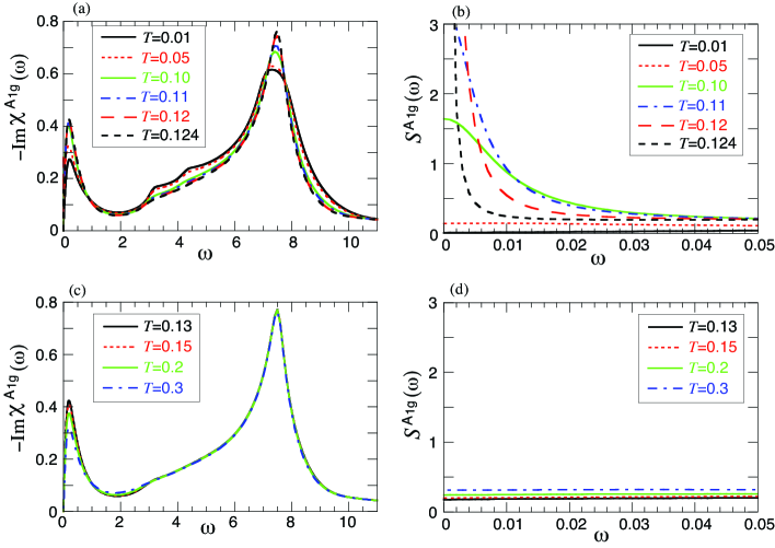
Figures 4(a) and 4(c) show ${\rm Im}\chi^{A1g}(\omega)$ on a large energy scale for temperatures below and above $T_{n}$, respectively. On this energy scale the temperature dependence of the spectra is quite weak. Since $\Pi^{A_{1g}3}=0$ for $T>T_{n}$ (see Sec. III A) the curves in Fig. 4(c) represent only the imaginary part of $\Pi^{A_{1g}A_{1g}}(\omega)$. They exhibit two well pronounced peaks. The main peak at $\omega\approx 7.5t$ arises from interband transitions near the ${\bf k}$-points $(\pi/4,3\pi/4)$ and $(3\pi/4,\pi/4)$ and the other peak at low energy is due to intraband transition. The curves in Fig. 4(a) include both terms in Eq. (32). However, the contribution from the second term is minor in the energy interval considered in the figure and the curves describe essentially $\Pi^{A_{1g}A_{1g}}(\omega)$.

Figures 4(b) and 4(d) show the $A_{1g}$ Raman intensity in a very small frequency interval near $\omega=0$. In these plots the low-frequency behavior of the $A_{1g}$ Raman scattering becomes visible which cannot be seen in the left panels because of their large energy scales. For $T>T_{n}$ the second term in Eq. (32) vanishes and there are no contributions from orbital nematic fluctuations even close to $T_{n}$. As a result the intensity is constant and very small at low frequencies. For $T<T_{n}$, on the other hand, orbital nematic fluctuations contribute substantially to the low-energy spectrum via the second term in Eq. (32) and lead to a large central peak when $T$ approaches $T_{n}$ from below.

III.2.3 B_2g Raman scattering and Lifshitz transition

Figure 5: (Color online) Panel (a) and (c): Im$\chi^{B_{2g}}(\omega)$ for temperatures below and above $T_{n}$, respectively. Panel (b) and (d): $S^{B_{2g}}(\omega)$ for the same temperatures.

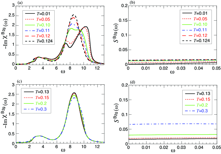
As we have discussed in Sec. III A orbital nematic fluctuations do not couple to the $B_{2g}$ component of Raman scattering which implies that the $B_{2g}$ spectrum is described only by $\Pi^{B_{2g}B_{2g}}(\omega)$, namely, by the first term in Eq. (32). As a result the Raman intensity at low frequencies becomes constant for all temperatures as shown in Figs. 5(b) and 5(d), similar as for the $A_{1g}$ symmetry at temperatures above $T_{n}$ [Fig. 4(d)]. The overall increase in the intensity with increasing temperature in Fig. 5(d), especially for the $T=0.3$ curve, is simply a result of the Bose factor in Eq. (17).

Figures 5(a) and 5(c) show the $B_{2g}$ Raman susceptibility on a large energy scale of the order of the band width. For $T>T_{n}$ practically no temperature dependence is visible and there is a peak around $8.5t$. The peak height is by a factor of 3-4 higher compared to the high-energy peak of the other symmetries [Figs. 3(a), 3(c), 4(a), 4(c)]. With decreasing temperature and entering the nematic phase [Fig. 5(a)] the peak shifts to higher energies. This is a manifestation of a Lifshitz transition. To understand the origin for this behavior we first note that the peak originates from interband transitions which are largest at the $X$ and $Y$ points because of the momentum dependence of the numerator in Eq. (64). In the normal state no interband transitions are possible at these points since both bands $\lambda_{{\bf k}}^{\pm}$ are located below the Fermi energy [Fig. 1(a)]. Instead, the dominant interband transitions occur a little away from the $X$ and $Y$ points where the upper band lies above and the lower band below the Fermi energy. Considering the phase space in the neighborhood of the $X$ point and the momentum dependence of the form factor in Eq. (64), the peak forms near $8.5t$ in the normal state. However, with decreasing temperature below $T_{n}$ the order parameter increases and the upper band at the $X$ point moves above the chemical potential which removes the pocket. Consequently strong transitions of about $10t$ are allowed near the $X$ point at low temperatures, which yields a peak around $10t$. As a result Fig. 5(a) exhibits a large shift of spectral weight towards higher energies at low temperatures. For the other symmetries the interband contribution to Raman scattering becomes zero at the $X$-point because of the momentum dependence of the form factor, which can be seen directly from Eqs. (60), (62), (63), (65). This explains why the Lifshitz transition due to the vanishing pocket at the $X$-point can only be seen in the $B_{2g}$ symmetry.

III.3 Properties of the central peak

Figure 6: (Color online) (a) Black, red, and dashed lines denote the intraband, interband and total contribution to ${\rm Im}\Pi^{33}(\omega)$, respectively. (b) Im$\Pi^{33}(\omega)$ for several temperatures.

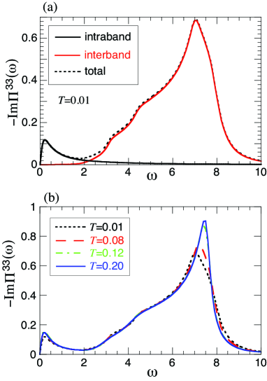
The central peak originates from the coupling to the nematic fluctuations described by Eq. (33). Hence the bare susceptibility for nematic fluctuations, $\Pi^{33}(\omega)$, is an important ingredient in our calculation. Its explicit expression Eq. (59) shows that it may be split into two different contributions, namely, an intraband contribution due to $A_{--}$ and $A_{++}$ and an interband contribution due to $A_{-+}$ and $A_{+-}$. The black and red lines in the upper panel in Fig. 6 show these two contributions for the imaginary part of $\Pi^{33}(\omega)$, the dashed line represents the total ${\rm Im}\Pi^{33}(\omega)$. The figure indicates that intra- and interband contributions are well separated in frequency: the first one is confined to low frequencies, increases first linearly in the frequency, passes through a maximum near $\omega\approx 2\delta$ and then decays rapidly with increasing frequency. On the other hand, the interband contribution is very small at small frequencies, rises with increasing frequency and shows a sharp maximum near $\omega\approx 7t$ due to strong transitions between the two bands near the point ${\bf k}=(\pi/2,\pi/2)$, see the band structure shown in Fig. 1(a). The interband contribution extends over a large frequency region comparable to the total band width. The lower panel in Fig. 6 shows ${\rm Im}\Pi^{33}(\omega)$ for several choices of temperatures. It depends in general only weakly on temperature and this holds both for the intra- and the interband contributions.

The second term in Eq. (32) exhibits a pole which describes in the static limit a nematic phase transition with a transition temperature $T_{n}$ determined by

$$1-g{\rm Re}\Pi^{33}(0)=0.$$ (51)

It is easy to show that $T_{n}$ coincides with the largest temperature where Eq. (16) has a non-vanishing solution for $n_{-}$, which is the usual definition of the transition temperature. Since the central peak emerges near $T=T_{n}$ and $\omega=0$, we take $T-T_{n}$ and $\omega$ as small quantities. Since $\Pi^{33}(\omega)$ depends only weakly on $T$ one may put in the expression

$${\rm Im}D^{33}(\omega)\approx g^{2}\frac{{\rm Im}\Pi^{33}(\omega)}{\left[1-g{\rm Re}\Pi^{33}(\omega)\right]^{2}+\left[g{\rm Im}\Pi^{33}(\omega)\right]^{2}}$$ (52)

everywhere $T=T_{n}$ except in the first term in the denominator. Writing

$${\rm Im}\Pi^{33}(\omega)\approx\alpha\omega$$ (53)

for small frequencies we obtain

$${\rm Im}D^{33}(\omega)\approx\frac{\omega/\alpha}{m^{2}(\omega)+\omega^{2}},$$ (54)

with

$$m^{2}(\omega)=\alpha^{-2}\left[{\rm Re}\Pi^{33}(0;T_{n})-{\rm Re}\Pi^{33}(\omega;T)\right]^{2},$$ (55)

where we denote the temperature dependence explicitly as a second argument in $\Pi^{33}$.

Putting in numbers one realizes that $m(0)$ is very small compared to one for the parameter range considered by us. One reason for this is that Re$\Pi^{33}$ depends only weakly on temperature which makes the numerator of $m^{2}(\omega)$ small. As a result the second term in Eq. (32) represents a low-energy contribution to the Raman susceptibility. Going over to the Raman scattering intensity Eq. (17) and taking the classical limit for the Bose function, $(1+b(\omega))/\pi\rightarrow T/(\pi\omega)$, we obtain approximately for the low-energy Raman response,

$$S^{\gamma}(\omega)\rightarrow-\frac{\left[{\rm Re}\Pi^{\gamma 3}(0;T_{n})\right]^{2}}{\pi\alpha}\cdot\frac{T_{n}}{m^{2}(\omega)+\omega^{2}}.$$ (56)

Neglecting the $\omega$-dependence of $m^{2}(\omega)$ the Raman intensity consists at low frequencies of a central peak of a Lorentzian shape with width $m(0)$; its peak height $S^{\gamma}(0)$ is proportional to $1/[\alpha m^{2}(0)]$. The area under the central peak thus becomes proportional to $1/(\alpha|m(0)|)=1/|{\rm Re}\Pi^{33}(0;T_{n})-{\rm Re}\Pi^{33}(0;T)|$. These results mean that in the limit $T\rightarrow T_{n}$ the width of the central peak vanishes as $|T-T_{n}|$ and that the peak height and the integrated spectral weight of the central peak diverge as $|T-T_{n}|^{-2}$ and $|T-T_{n}|^{-1}$, respectively.

The asymptotic formula Eq. (56) contains the parameter $\alpha$ which was introduced in Eq. (53). $\alpha$ is determined by intraband scattering processes [Fig. 6(a)] which owe their existence to a finite value of $\delta$ in Eqs. (10)-(12) and (39)-(41). In fact, in the limit $\delta\rightarrow 0$ $\alpha$ diverges and the width of the central peak vanishes even for $T\neq T_{n}$. However, the integrated spectral weight of the central peak is proportional to $1/|{\rm Re}\Pi^{33}(0;T_{n})-{\rm Re}\Pi^{33}(0;T)|$ and thus independent of $\alpha$. Moreover, it is in general rather large because ${\rm Re}\Pi^{33}$ depends only weakly on temperature. Because of the rather weak $\delta$ dependence of Re$\Pi^{\gamma 3}(0;T_{n})$, we thus find the remarkable result that the emergence of the central peak and its spectral weight are essentially independent of the damping $\delta$.

The above analysis assumes tacitly that the linear approximation for ${\rm Im}\Pi^{33}(\omega)$ [Eq. (53)] is valid over the region where the central peak is substantially different from zero. The maximum of ${\rm Im}\Pi^{33}$ lies near $2\delta$ and is rather independent of $\delta$. Thus the linear approximation holds well in the interval $[0,2\delta]$ and we have according to Fig. 6 $\alpha\sim-0.1/\delta$. Our analysis therefore requires that $m(0)\ll 2\delta$ or that $|{\rm Re}\Pi^{33}(0,T_{n})-{\rm Re}\Pi^{33}(0,T)|\ll 0.2$, which is well fulfilled close to $T_{n}$.

III.4 Coulomb screening

It is known that the long-range Coulomb interaction may strongly screen the first diagram in Fig. 2(a) in the $A_{1g}$ channel.M. V. Klein and S. B. Dierker (1984); H. Monien and A. Zawadowski (1990); Devereaux and Hackl (2007) This screening effect was discussed for iron pnictides in the superconducting state and different conclusions have been obtained: In Refs. G. R. Boyd, T. P. Devereaux, P. J. Hirschfeld, V. Mishra, and D. J. Scalapino, 2009 and I. I. Mazin, T. P. Devereaux, J. G. Analytis, J.-H. Chu, I. R. Fisher, B. Muschler and R. Hackl, 2010 screeening was found to be important whereas in Ref. A. V. Chubukov, I. Eremin, and M. M. Korshunov, 2009 it was shown that it vanishes under plausible assumptions. In the present section we study Coulomb screening in the normal and nematic state. The corresponding diagram is given by the second diagram in Fig. 2(a) by replacing $\hat{\tau}_{3}$ by $\hat{\tau}_{0}$ and the coupling constant $g$ by the bare Coulomb potential $V({\bf q})$ where $\bf q$ is the momentum of the incident photon. Taking the limit ${\bf q}\rightarrow 0$ the additional contribution due to Coulomb screening is given by

$$-\Pi^{\gamma 0}(\omega)\frac{1}{\Pi^{00}(\omega)}\Pi^{0\gamma}(\omega)\,.$$ (57)

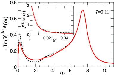
The explicit calculation of Eq. (57) shows that the bubbles in this expression contain only intraband scattering processes and thus may become relevant only at low energy, similar as in the case of Fig. 6(a). Figure 7 shows for a representative case $A_{1g}$ spectra with (solid line) and without (dashed line) Coulomb screening. As expected the two curves are very similar or practical identical at energies larger than about $t$ whereas the height of the low-energy maximum near $0.2t$ is noticeably reduced by screening. The inset in Fig. 7 exhibits the scattering intensity $S^{A_{1g}}(\omega)$ on a very low energy scale. In this range $S^{A_{1g}}$ is mainly determined by the second term in Eq. (32) which is unaffected by Coulomb screening. This implies that the presence and the spectral form of the central mode is insensitive to Coulomb screening. The term in Eq. (57) enters $S^{A_{1g}}$ in the inset of Fig. 7 only via a hardly visible reduction of the constant background. In the normal state $\Pi^{\gamma 0}(\omega)$ is zero for $\gamma=B_{1g}$ and $B_{2g}$ so that these channels are unaffected by the Coulomb interaction in this case. On the other hand, $\Pi^{\gamma 0}(\omega)$ is nonzero for $\gamma=B_{1g}$ in the nematic state (see Sec. III A). However, we find that the resulting changes in Fig. 3 would be invisibly small. We also have considered corrections of the nematic fluctuations due to the Coulomb interaction, i.e., where the propagator $D^{33}(\omega)$ in Eq. (33) contains contributions from $\Pi^{00}(\omega)$ due to the non-vanishing $\Pi^{30}(\omega)$ in the nematic state. We found that these effects are very small and do not change substantially the presented results in the nematic state.

Figure 7: (Color online) Comparison of the $A_{1g}$ spectra with (solid line) and without (dashed line) Coulomb screening. The dashed line is identical with the curve for $T=0.11$ in Fig. 4.

IV Conclusions

Our analysis shows that low-energy orbital fluctuations near the nematic transition temperature $T_{n}$ can produce a central peak in the Raman intensity $S^{\gamma}(\omega)$. Depending on the symmetry this central peak may appear both above and below $T_{n}$ as in the case of the $B_{1g}$ spectrum, only below $T_{n}$ as for the $A_{1g}$ or not at all as for the $B_{2g}$ spectrum. The area under the central peak diverges as $|T-T_{n}|^{-1}$ and the peak width becomes narrower as $|T-T_{n}|$. While our theory contains the damping $\delta$ of the electrons, we have found that the integrated spectral weight of the central peak does not depend essentially on $\delta$. The predicted selection rules and properties of the central peak may be helpful to detect orbital fluctuations in Raman spectra.

After the present work was completed we became aware of recent Raman scattering experiments in Ba(Fe_1-xCo_x)₂As₂ near the SDW phase.gal The authors found a strong enhancement of the scattering intensity at low energies around the tetragonal-orthorhombic structural phase transition in the $B_{1g}$ channel. Their data are consistent with our results [see Figs. 3(b) and 3(d)], indicating that orbital nematic fluctuations become strong near the structural phase transition. It would be interesting to perform also Raman scattering measurements in the $B_{2g}$ and $A_{1g}$ channels in the small temperature region bounded by the structural phase transition and the SDW phase. The energy range where the enhancement of low-energy spectral weight was observed is, however, much wider than in our theoretical spectra Figs. 3(b) and 3(d), if we assume $t\sim 150$ meV. This quantitative difference cannot be resolved by invoking a larger damping constant $\delta$ in our model. It could mean that more realistic self-energies must be included in the calculations.

Quite recently magnetic torque measurements revealed the breaking of the fourfold symmetry far away from the SDW instability. As an explanation the occurrence of an orbital nematic instability was discussed. S. Kasahara, H. J. Shi, K. Hashimoto, S. Tonegawa, Y. Mizukami, T. Shibauchi, K. Sugimoto, T. Fukuda, T. Terashima, A. H. Nevidomskyy, and Y. Matsuda (2012) It is highly desirable to perform Raman scattering measurements around the nematic critical temperatures measured by the magnetic torque experiments and to confirm the presence of nematic fluctuations.

Raman scattering in the high energy region involves mainly individual particle-hole excitations. At low temperatures the nematic distortion may become large enough to induce a Lifshitz transition where the Fermi pocket at the $X$- or the $Y$-point disappears. As a result particle-hole excitations at the $X$-point are allowed to occur. The resulting upward shift of spectral weight in the Raman intensity should be observable at high frequencies in the $B_{2g}$, but not in the $A_{1g}$ or $B_{1g}$ Raman spectra.

Appendix

A general formula for the bare susceptibilities has been given in Eq. (42). By suitably specifying the components of the general vertices in Eqs. (34) and (35) one finds for each susceptibility a more explicit expression by computing the dot product of the four-dimensional vectors ${\bf G}$ in Eq. (42). It is convenient to introduce the abbreviations

$$A_{\sigma\sigma^{\prime}}=\frac{\delta}{(\epsilon+\omega-\lambda_{\bf k}^{\sigma})^{2}+\delta^{2}}\cdot\frac{\delta}{(\epsilon-\lambda_{\bf k}^{\sigma^{\prime}})^{2}+\delta^{2}},$$ (58)

for $\sigma=\pm,\sigma^{\prime}=\pm$. The arguments $\epsilon,\omega,{\bf k}$ have been dropped for simplicity. We obtain,

$${\rm Im}\Pi^{33}(\omega)=\frac{2}{\pi N}\sum_{\bf k}\int d\epsilon\left[f(\epsilon+\omega)-f(\epsilon)\right]$$

$$\hskip 56.9055pt\times\left[\frac{(\xi_{\bf k}^{-})^{2}}{E_{\bf k}^{2}}(A_{++}+A_{--})+\frac{(\epsilon_{\bf k}^{12})^{2}}{E_{\bf k}^{2}}(A_{+-}+A_{-+})\right];$$ (59)

$${\rm Im}\Pi^{B_{1g}3}(\omega)=\frac{2}{\pi N}\sum_{\bf k}\int d\epsilon\left[f(\epsilon+\omega)-f(\epsilon)\right]$$

$$\hskip 56.9055pt\times\left\{\left[\gamma_{0}^{B_{1g}}\frac{\xi_{\bf k}^{-}}{E_{\bf k}}+\gamma_{3}^{B_{1g}}\frac{(\xi_{\bf k}^{-})^{2}}{E_{\bf k}^{2}}\right]A_{++}+\gamma_{3}^{B_{1g}}\frac{(\epsilon_{\bf k}^{12})^{2}}{E_{\bf k}^{2}}(A_{+-}+A_{-+})\right.$$

$$\hskip 199.16928pt+\left.\left[-\gamma_{0}^{B_{1g}}\frac{\xi_{\bf k}^{-}}{E_{\bf k}}+\gamma_{3}^{B_{1g}}\frac{(\xi_{\bf k}^{-})^{2}}{E_{\bf k}^{2}}\right]A_{--}\right\};$$ (60)

$${\rm Im}\Pi^{B_{2g}3}(\omega)=\frac{2}{\pi N}\sum_{\bf k}\int d\epsilon\left[f(\epsilon+\omega)-f(\epsilon)\right]$$

$$\hskip 56.9055pt\times\left[\left(\gamma_{0}^{B_{2g}}\frac{\xi_{\bf k}^{-}}{E_{\bf k}}+\gamma_{1}^{B_{2g}}\frac{\epsilon_{\bf k}^{12}\xi_{\bf k}^{-}}{E_{\bf k}^{2}}\right)A_{++}-\gamma_{1}^{B_{2g}}\frac{\epsilon_{\bf k}^{12}\xi_{\bf k}^{-}}{E_{\bf k}^{2}}(A_{+-}+A_{-+})\right.$$

$$\hskip 199.16928pt+\left.\left(-\gamma_{0}^{B_{2g}}\frac{\xi_{\bf k}^{-}}{E_{\bf k}}+\gamma_{1}^{B_{2g}}\frac{\epsilon_{\bf k}^{12}\xi_{\bf k}^{-}}{E_{\bf k}^{2}}\right)A_{--}\right];$$ (61)

this susceptibility vanishes both in the normal and in the nematic state because the integrand contains a form factor $\sin k_{x}\sin k_{y}$ (see also Sec. III A for a symmetry-based argument);

$${\rm Im}\Pi^{A_{1g}3}(\omega)=\frac{2}{\pi N}\sum_{\bf k}\int d\epsilon\left[f(\epsilon+\omega)-f(\epsilon)\right]$$

$$\hskip 56.9055pt\times\left\{\left[\gamma_{0}^{A_{1g}}\frac{\xi_{\bf k}^{-}}{E_{\bf k}}+\gamma_{1}^{A_{1g}}\frac{\epsilon_{\bf k}^{12}\xi_{\bf k}^{-}}{E_{\bf k}^{2}}+\gamma_{3}^{A_{1g}}\frac{(\xi_{\bf k}^{-})^{2}}{E_{\bf k}^{2}}\right]A_{++}\right.$$

$$\hskip 99.58464pt+\left[-\gamma_{1}^{A_{1g}}\frac{\epsilon_{\bf k}^{12}\xi_{\bf k}^{-}}{E_{\bf k}^{2}}+\gamma_{3}^{A_{1g}}\frac{(\epsilon_{\bf k}^{12})^{2}}{E_{\bf k}^{2}}\right](A_{+-}+A_{-+})$$

$$\hskip 142.26378pt+\left.\left[-\gamma_{0}^{A_{1g}}\frac{\xi_{\bf k}^{-}}{E_{\bf k}}+\gamma_{1}^{A_{1g}}\frac{\epsilon_{\bf k}^{12}\xi_{\bf k}^{-}}{E_{\bf k}^{2}}+\gamma_{3}^{A_{1g}}\frac{(\xi_{\bf k}^{-})^{2}}{E_{\bf k}^{2}}\right]A_{--}\right\};$$ (62)

this susceptibility is zero if $n_{-}$ is zero, i.e., in the normal state because the integrand contains a form factor $\cos k_{x}-\cos k_{y}$ (see also Sec. III A); $\Pi^{3\gamma}$ becomes equal to $\Pi^{\gamma 3}$;

$${\rm Im}\Pi^{B_{1g}B_{1g}}(\omega)=\frac{2}{\pi N}\sum_{\bf k}\int d\epsilon\left[f(\epsilon+\omega)-f(\epsilon)\right]$$

$$\hskip 56.9055pt\times\left[\left(\gamma_{0}^{B_{1g}}+\gamma_{3}^{B_{1g}}\frac{\xi_{\bf k}^{-}}{E_{\bf k}}\right)^{2}A_{++}+\left(\gamma_{3}^{B_{1g}}\frac{\epsilon_{\bf k}^{12}}{E_{\bf k}}\right)^{2}(A_{+-}+A_{-+})\right.$$

$$\hskip 199.16928pt+\left.\left(\gamma_{0}^{B_{1g}}-\gamma_{3}^{B_{1g}}\frac{\xi_{\bf k}^{-}}{E_{\bf k}}\right)^{2}A_{--}\right];$$ (63)

$${\rm Im}\Pi^{B_{2g}B_{2g}}(\omega)=\frac{2}{\pi N}\sum_{\bf k}\int d\epsilon\left[f(\epsilon+\omega)-f(\epsilon)\right]$$

$$\hskip 56.9055pt\times\left[\left(\gamma_{0}^{B_{2g}}+\gamma_{1}^{B_{2g}}\frac{\epsilon_{\bf k}^{12}}{E_{\bf k}}\right)^{2}A_{++}+\left(\gamma_{1}^{B_{2g}}\frac{\xi_{\bf k}^{-}}{E_{\bf k}}\right)^{2}(A_{+-}+A_{-+})\right.$$

$$\hskip 199.16928pt+\left.\left(\gamma_{0}^{B_{2g}}-\gamma_{1}^{B_{2g}}\frac{\epsilon_{\bf k}^{12}}{E_{\bf k}}\right)^{2}A_{--}\right];$$ (64)

$${\rm Im}\Pi^{A_{1g}A_{1g}}(\omega)=\frac{2}{\pi N}\sum_{\bf k}\int d\epsilon\left[f(\epsilon+\omega)-f(\epsilon)\right]$$

$$\hskip 28.45274pt\times\left\{\left[\left(\gamma_{0}^{A_{1g}}+\gamma_{3}^{A_{1g}}\frac{\xi_{\bf k}^{-}}{E_{\bf k}}\right)^{2}+\left(\gamma_{0}^{A_{1g}}+\gamma_{1}^{A_{1g}}\frac{\epsilon_{\bf k}^{12}}{E_{\bf k}}\right)^{2}+2\gamma_{1}^{A_{1g}}\gamma_{3}^{A_{1g}}\frac{\epsilon_{\bf k}^{12}\xi_{\bf k}^{-}}{E_{\bf k}^{2}}-\left(\gamma_{0}^{A_{1g}}\right)^{2}\right]A_{++}\right.$$

$$\hskip 36.98857pt+\left.\left[\left(\gamma_{0}^{A_{1g}}-\gamma_{3}^{A_{1g}}\frac{\xi_{\bf k}^{-}}{E_{\bf k}}\right)^{2}+\left(\gamma_{0}^{A_{1g}}-\gamma_{1}^{A_{1g}}\frac{\epsilon_{\bf k}^{12}}{E_{\bf k}}\right)^{2}+2\gamma_{1}^{A_{1g}}\gamma_{3}^{A_{1g}}\frac{\epsilon_{\bf k}^{12}\xi_{\bf k}^{-}}{E_{\bf k}^{2}}-\left(\gamma_{0}^{A_{1g}}\right)^{2}\right]A_{--}\right.$$

$$\hskip 199.16928pt+\left.\left(\gamma_{1}^{A_{1g}}\frac{\xi_{\bf k}^{-}}{E_{\bf k}}-\gamma_{3}^{A_{1g}}\frac{\epsilon_{\bf k}^{12}}{E_{\bf k}}\right)^{2}(A_{+-}+A_{-+})\right\}.$$ (65)