Flexoelectricity from density-functional perturbation theory

Abstract

We derive the complete flexoelectric tensor, including electronic and lattice-mediated effects, of an arbitrary insulator in terms of the microscopic linear response of the crystal to atomic displacements. The basic ingredient, which can be readily calculated from first principles in the framework of density-functional perturbation theory, is the quantum-mechanical probability current response to a long-wavelength acoustic phonon. Its second-order Taylor expansion in the wavevector ${\bf q}$ around the $\Gamma$ (${\bf q}=0$) point in the Brillouin zone naturally yields the flexoelectric tensor. At order one in ${\bf q}$ we recover Martin’s theory of piezoelectricity [R. M. Martin, Phys. Rev. B 5, 1607 (1972)], thus providing an alternative derivation thereof. To put our derivations on firm theoretical grounds, we perform a thorough analysis of the nonanalytic behavior of the dynamical matrix and other response functions in a vicinity of $\Gamma$. Based on this analysis, we find that there is an ambiguity in the specification of the “zero macroscopic field” condition in the flexoelectric case; such arbitrariness can be related to an analytic band-structure term, in close analogy to the theory of deformation potentials. As a byproduct, we derive a rigorous generalization of the Cochran-Cowley formula [W. Cochran and R. A. Cowley, J. Phys. Chem. Solids ${\bf 23}$, 447 (1962)] to higher orders in ${\bf q}$. This can be of great utility in building reliable atomistic models of electromechanical phenomena, as well as for improving the accuracy of the calculation of phonon dispersion curves. Finally, we discuss the physical interpretation of the various contributions to the flexoelectric response, either in the static or dynamic regime, and we relate our findings to earlier theoretical works on the subject.

I Introduction

Flexoelectricity, the electric polarization linearly induced by an inhomogeneous deformation, Kogan (1964) has become a popular topic in material science during the past few years Cross (2006); Zubko et al. (2007); Lee et al. (2011); Catalan et al. (2011); Lu et al. (2012); Nguyen et al. (2013); Zubko et al. (2013). The interest is motivated by the universality of the flexoelectric effect, which, unlike piezoelectricity, is present in insulators of any symmetry and composition (including simple solids such as crystalline Si and NaCl).  While flexoelectricity is not a new discovery (the effect was predicted by Kogan in 1964 Kogan (1964); the bending of a parallel-plate capacitor induced by an applied voltage was experimentally demonstrated in 1968 by Bursian et al. Bursian and Zaikovskii (1968)), it has traditionally been regarded as a very weak effect, hardly detectable in macroscopic samples. Only in the past few years research has taken off on this front, thanks to the breathtaking progress in the design and control of nanoscale structures. From an application point of view, reducing the size of the active elements is crucial to obtaining a sufficiently large response: The uniform strain gradient that can be sustained by a sample before material failure is inversely proportional to its lateral dimensions. Ironically, in the context of perovskite thin films, strain gradients (e.g. occurring during epitaxial growth) have long been regarded as harmful to the operation of ferroelectric memories, Catalan et al. (2005); Dawber et al. (2005) and only later explored as a potentially useful functional property. Several recent experimental breakthroughs Zubko et al. (2007); Catalan et al. (2011); Lu et al. (2012) have convincingly demonstrated that the effect can indeed be giant Lee et al. (2011) in thin films, large enough to rotate Catalan et al. (2011) and/or switch Lu et al. (2012) ferroelectric domains, or to replace conventional piezoelectric materials Fousek et al. (1999); Zhu et al. (2006) in sensors and transducers.

At the level of the theory, advances have been comparatively slow. For a long time, the main reference in the field was the seminal work by Tagantsev Tagantsev (1986), which focused on lattice-mediated responses only, and from a phenomenological perspective. Maranganti and Sharma Maranganti and Sharma (2009) have later applied the method of Ref. Tagantsev, 1986 to the calculation of the flexoelectric coefficients in selected materials. Unfortunately, a considerable spread emerged between the predictions of different microscopic models, hence the need for a more fundamental treatment. It has taken many years before a full first-principles calculation of the flexoelectric coefficients was attempted Hong et al. (2010). More recently Resta Resta (2010), and Hong and Vanderbilt Hong and Vanderbilt (2011) have established the basis for a general formulation of the problem in the context of electronic-structure density functional theory, but a unified approach, encompassing both electronic and lattice-mediated effects, has not emerged yet. Note that most theoretical treatments to date have defined the flexoelectric tensors starting from the real-space moments of localized response functions (either atomic forces induced on neighboring atoms Tagantsev (1986) or multipolar expansions of the charge response to atomic displacements Resta (2010)). This is a drawback in the context of electronic-structure calculations, where working with periodic functions would be preferable, as it would eliminate the need for expensive supercell geometries.

Given the incomplete state of the theory, there are pressing questions coming from the experiments that are still unresolved to date. First, whether the flexoelectric tensor is a well-defined bulk property has been a matter of debate for several years; Resta (2010); Tagantsev (1986) consequently, it is currently unclear if it is at all possible to separate the surface and bulk contributions in a typical experiment. Next, it has been pointed out Zubko et al. (2007) that static measurements alone leave the flexoelectric tensor undetermined – in order to solve for all the independent components one needs to combine static with dynamic data. Is it, however, physically justified to “mix” the two? What do we get as a result, a static or a dynamic quantity? Finally, of particular importance in the area of perovskite oxides (which are by far the best studied and most promising materials for flexoelectric applications) is the interplay of inhomogeneous deformations with the main order parameters (either ferroelectric polarization or antiferrodistortive tilts of the oxygen octahedral network). This has been the subject of several studies in the context of phenomenological Morozovska et al. (2012a, b) and effective Hamiltonian Ponomareva et al. (2012) approaches, but a systematic way to calculate the coupling coefficients (to be used as an input to the higher-level simulations) is still missing.

In a broader context, it worth noting that the interest of flexoelectricity is by no means limited to perovskites: For example, curvature-induced effects are of outstanding relevance in the physics of two-dimensional nanostructures Ortix et al. (2011) such as $sp^{2}$-bonded crystals (e.g. graphene Kalinin and Meunier (2008) or boron nitride Naumov et al. (2009)). Also, the electrostatic potential induced by deformation fields is a known concern in the performance of optoelectronic quantum-well devices, Lew Yan Voon and Willatzen (2011) especially in the promising area of foldable inorganic light-emitting diodes. Park et al. (2010) The theory of absolute deformation potentials, Van de Walle (1989) intimately related to flexoelectricity, Resta et al. (1990); Resta (2010) is an invaluable tool in the band-gap engineering of these (and other) semiconductor-based systems. Rationalizing these diverse and technologically important phenomena into a unified theory would be, of course, highly desirable from a modeling perspective.

Here we show how to consistently address the above issues by using density functional perturbation theory Baroni et al. (2001) (DFPT) as a methodological framework. By taking the long-wavelength limit of acoustic phonons, we derive the electromechanical tensors (both piezoelectric and flexoelectric) in terms of standard lattice-periodic response functions, which can be readily calculated by means of publicly available first-principles codes. We demonstrate the consistency of our formalism by rederiving already established results, such as Martin’s theory Martin (1972) of piezoelectricity and existing theories Tagantsev (1986); Resta (2010); Hong and Vanderbilt (2011) of flexoelectricity. To substantiate our arguments, we carefully study the nonanalyticities, due to the long-range character of the electrostatic interactions, that plague the electronic response functions in the long-wave regime. In particular, we devise a rigorous strategy to dealing with this issue by suppressing the macroscopic (${\bf G}=0$) component of the self-consistent electrostatic potential in the linear response calculations. We find, however, that such a procedure is not unique – there is an inherent ambiguity in the specification of the “zero macroscopic field” condition in the flexoelectric case, which can be traced back to the choice of an arbitrary reference energy in the periodic crystal. We rationalize such ambiguity by establishing a formal link between the present theory of flexoelectricity and the preexisting theory of absolute deformation potentials. Resta et al. (1990) In addition to providing a solid formal basis to our derivations, our treatment of macroscopic electrostatics also yields a rigorous generalization of the Cochran-Cowley formula to higher orders in ${\bf q}$, which can be of great utility in future lattice-dynamical studies. Finally, based on our findings, (i) we derive an exact sum rule, relating the flexoelectric coefficients to the macroscopic elastic tensor; (ii) we use such a sum rule to demonstrate that the same definition of the flexoelectric tensor is equally well suited to describing static or dynamic phenomena; (iii) we discuss the physical interpretation of the various physical contributions to the flexoelectric tensor, relating them to earlier first-principles Resta et al. (1990) and phenomenological Morozovska et al. (2012a, b) studies.

This work is structured as follows. In Section II we introduce some useful basic concepts of continuum mechanics, and the general strategy that we use to attack the flexoelectric problem. In Section III we introduce the formalism of density-functional perturbation theory, and the basic ingredients that will be used in the remainder of this work. In Section IV we proceed to performing the long-wave analysis of an acoustic phonon, deriving the piezoelectric and flexoelectric response tensors in terms of the basic ingredients defined above. In Section V we discuss several important properties of the electronic response functions (polarization and charge density), and use them to draw a formal connection to Martin’s theory of piezoelectricity, Martin (1972) and to earlier theories Hong and Vanderbilt (2011); Resta (2010); Tagantsev (1986) of flexoelectricity. In Section VI we study the nonanalytic properties of the aforementioned response functions, obtaining (among other results) a higher-order generalization of the lattice-dynamical theory of Pick, Cohen and Martin. Pick et al. (1970) Finally, Section VII is devoted to discussing the physical implications of the derived formulas, while in Section VIII we briefly summarize our main results and conclusions.

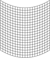
$\eta_{1,11}$	$\eta_{2,11}$
$\varepsilon_{11,1}$	$\varepsilon_{12,1}=\varepsilon_{21,1}$
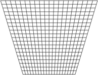
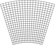
$\eta_{1,12}=\eta_{1,21}$	$\varepsilon_{11,2}$

Figure 1: Individual components of the strain gradient tensor in a square two-dimensional lattice. The “longitudinal” ($\varepsilon_{1,11}$), “shear” ($\varepsilon_{12,1}$) and “transverse” (or “bending”, $\varepsilon_{11,2}$) components are linearly independent; a fourth pattern of less obvious physical interpretation ($\eta_{1,12}$) is a combination of $\varepsilon_{12,1}$ and $\varepsilon_{11,2}$. Direction 1 corresponds to the horizontal axis, 2 to the vertical; the polarization vector is oriented along 2.

II Preliminaries

II.1 Strain and strain gradients

In continuum mechanics, a deformation can be expressed as a three-dimensional (3D) vector function, $u_{\alpha}({\bf r})$, describing the displacement of a material point from its reference position at ${\bf r}$ to its current location ${\bf r}^{\prime}$,

$$r_{\alpha}^{\prime}({\bf r})=r_{\alpha}+u_{\alpha}({\bf r}),$$

The deformation gradient is defined as the gradient of $u_{\alpha}$ taken in the reference configuration,

$$\tilde{\varepsilon}_{\alpha\beta}({\bf r})=u_{\alpha,\beta}({\bf r})=\frac{\partial u_{\alpha}({\bf r})}{\partial r_{\beta}}.$$ (1)

$\tilde{\varepsilon}_{\alpha\beta}({\bf r})$ is often indicated in the literature as “unsymmetrized strain tensor”, as it generally contains a proper strain plus a rotation. By symmetrizing its indices one can remove the rotational component, thus obtaining the symmetrized strain tensor,

$$\varepsilon_{\alpha\beta}=\frac{1}{2}\left(u_{\alpha,\beta}+u_{\beta,\alpha}\right).$$

$\varepsilon_{\alpha\beta}$ is a convenient measure of local strain, as it only depends on relative displacements of two adjacent material points, and not on their absolute translation or rotation with respect to some reference configuration.

In this work we shall be primarily concerned with the effects of a spatially inhomogeneous strain. The third-rank strain gradient tensor can be defined in two different ways, both important for the derivations that follow. The first (type-I) form consists in the gradient of the unsymmetrized strain,

$$\eta_{\alpha,\beta\gamma}({\bf r})=\frac{\partial\tilde{\varepsilon}_{\alpha\beta}({\bf r})}{\partial r_{\gamma}}=\frac{\partial^{2}u_{\alpha}({\bf r})}{\partial r_{\beta}\partial r_{\gamma}}.$$ (2)

Note that $\eta_{\alpha,\beta\gamma}$, manifestly invariant upon $\beta\leftrightarrow\gamma$ exchange, corresponds to the $\nu_{\alpha\beta\gamma}$ tensor of Ref. Hong and Vanderbilt, 2011, and to the symbol $\partial\epsilon_{\alpha\beta}/\partial r_{\gamma}$ of Ref. Tagantsev, 1986. Alternatively, the strain gradient tensor can be defined (type-II) as the gradient of the symmetric strain, $\varepsilon_{\alpha\beta}$,

$$\varepsilon_{\alpha\beta,\gamma}({\bf r})=\frac{\partial\varepsilon_{\alpha\beta}({\bf r})}{\partial r_{\gamma}},$$

invariant upon $\alpha\leftrightarrow\beta$ exchange. It is straightforward to verify that the two tensors contain exactly the same number of independent entries, and that a one-to-one relationship can be established to express the former as a function of the latter and viceversa. For example,

$$\eta_{\alpha,\beta\gamma}=\varepsilon_{\alpha\beta,\gamma}+\varepsilon_{\gamma\alpha,\beta}-\varepsilon_{\beta\gamma,\alpha}.$$ (3)

In Fig. 1 we illustrate the three independent components of the $\eta_{\alpha,\beta\gamma}$ and $\varepsilon_{\alpha\beta,\gamma}$ tensors on a square two-dimensional (2D) lattice, evidencing analogies and differences. It is clear from the figure that the longitudinal and shear components are elementary objects in both type-I and type-II forms. The main difference between the two representations concerns the third independent component, which assumes the form of a flat displacement pattern in the type-I form, and has the more intuitive interpretation of a pure bending (one can show that $\varepsilon_{11,2}=1/R$, where $R$ is the curvature radius) in the type-II form; the latter will be indicated as transverse strain gradient henceforth. In fact, these three components of the strain gradient tensor are, by symmetry, the only types of independent perturbations in a cubic material, and are therefore very important in the context of flexoelectricity.

II.2 Long-wavelength acoustic phonons

A macroscopic strain gradient breaks the translational symmetry of the crystal lattice. For this reason, the response to such a perturbation cannot be straightforwardly represented in periodic boundary conditions. This makes the theoretical study of flexoelectricity more challenging than other forms of electromechanical couplings, e.g. piezoelectricity. To circumvent this difficulty, we shall base our analysis on the study of long-wavelength acoustic phonons. These perturbations, while generally incommensurate with the crystal lattice, can be conveniently described Baroni et al. (2001), in terms of functions that are lattice-periodic, and therefore are formally and computationally very advantageous.

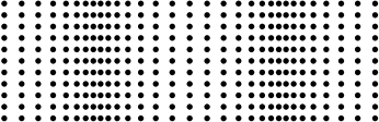
Figure 2: Displacement fields in longitudinal (top) and transversal (bottom) sound waves.

The direct relationship between an acoustic phonon and a mechanical deformation is clear from Fig. 2: in the longitudinal and transversal waves one can visually identify regions of negative and positive strain gradients, respectively of the longitudinal and shear type. Mathematically, this observation can be formalized by writing (at the lowest order in the wavevector ${\bf q}$) an acoustic phonon as a homogeneous displacement of every material point of the type

$$u_{\beta}({\bf r},t)=U_{\beta}\,e^{i{\bf q}\cdot{\bf r}-i\omega t},$$

where $U_{\beta}$ is the displacement amplitude and $\omega$ the frequency. Consider now the microscopic polarization currents (these are due to the displacements of the charged particles, electron and nuclei, from their equilibrium positions) induced by the phonon at the linear-response level, 

$$\tilde{P}_{\alpha}({\bf r},t)=U_{\beta}\tilde{P}^{\bf q}_{\alpha\beta}({\bf r})\,e^{i{\bf q}\cdot{\bf r}-i\omega t}.$$

Assuming for the moment that $\tilde{P}^{\bf q}$ is an analytic function of ${\bf q}$ at the $\Gamma$ point, in a neighborhood of $\Gamma$ (i.e. in the long-wavelength regime) we can replace it with its second-order Taylor expansion,

$$\tilde{P}^{\bf q}_{\alpha\beta}\simeq\tilde{P}^{(0)}_{\alpha\beta}-iq_{\gamma}\tilde{P}^{(1,\gamma)}_{\alpha\beta}-\frac{q_{\gamma}q_{\lambda}}{2}\tilde{P}^{(2,\gamma\lambda)}_{\alpha\beta}.$$ (4)

Now, by applying Eq. (1) and Eq. (2), we can compute the local deformation gradient and strain gradient that are associated with the acoustic phonon,

$$\tilde{\varepsilon}_{\beta\gamma}({\bf r},t) = \frac{\partial u_{\beta}}{\partial r_{\gamma}}=iU_{\beta}q_{\gamma}\,e^{i{\bf q}\cdot{\bf r}-i\omega t},$$ (5)

$$\eta_{\beta,\gamma\lambda}({\bf r},t) = \frac{\partial^{2}u_{\beta}}{\partial r_{\gamma}\partial r_{\lambda}}=-U_{\beta}q_{\gamma}q_{\lambda}\,e^{i{\bf q}\cdot{\bf r}-i\omega t}.$$ (6)

A comparison of Eqs. (4), (5) and (6) suggests that the polarization response to a uniform strain (piezoelectricity) and to a strain-gradient (flexoelectricity) are, respectively, related to the first- and second-order Taylor expansion in powers of ${\bf q}$ of the polarization field produced by a sound wave. The latter can be computed by working with lattice-periodic functions only, implying that all the theoretical and computational weaponry developed so far within periodic boundary conditions (e.g. Bloch theorem, plane wave basis set, pseudopotentials, etc.) can be proficiently applied to the flexoelectric problem. This is precisely the approach that we shall take in the remainder of this work.

While this appears conceptually simple, there are a number of important issues that need to be addressed before one can establish the formal link between the electrical properties of sound waves and the macroscopic electromechanical tensors. First of all, it is not clear a priori whether the above strategy is even applicable. Long-wavelength phonons are generally accompanied by macroscopic electric fields. This is a substantial complication from the operational point of view: the longitudinal character of the electrostatic screening causes a nonanalytic behavior of most response functions (e.g. the atomic eigendisplacements and the electronic polarization, see Section VI for a detailed discussion) in a vicinity of $\Gamma$, thwarting their expansion in powers of ${\bf q}$. Whether (and how) these nonanalyticities can be tamed will need to be assessed prior to starting the actual derivations. Second, phonon eigenmodes also contain, in addition to genuine macroscopic deformations, translations and rotations of a given crystal cell with respect to its reference configuration at rest. It will be therefore necessary to show that such rototranslations do not contribute to the macroscopic electrical response. Third, a phonon is inherently a dynamic perturbation, and whether the effects derived for a sound wave are equally applicable to a static deformation will need to be carefully demonstrated. In the following Sections we shall first introduce the basic ingredients that we need in order to derive the total polarization response, Eq. (4); next, we shall proceed to the formal derivation of the electromechanical tensors, and to their validation in relation to the aforementioned sources of concern.

III Density-functional perturbation theory

This Section will provide a brief introduction to the DFPT formalism. This is mainly aimed at specifying the general context of our derivations, as well as at pointing out the key modifications to the standard approach Baroni et al. (2001) that are necessary in the context of this work. In particular, we shall put the emphasis on the following three technical points: the treatment of the macroscopic fields; the definition of the microscopic polarization response; the practical calculation of the relevant response functions by means of publicly available codes.

III.1 Linear response to monochromatic perturbations

Our starting point is an insulating crystal, whose equilibrium configuration is described by the three primitive translation vectors, ${\bf a}_{1,2,3}$, and by a basis of $N$ atoms located at positions $\bm{\tau}_{\kappa}$ ($\kappa=1,\ldots,N$) within the primitive unit cell. Within density-functional theory, the electronic ground state can be written in terms of the self-consistent (SCF) Kohn-Sham equation,

$$\hat{H}_{\bf k}|\phi_{n{\bf k}}\rangle=\epsilon_{n{\bf k}}|\phi_{n{\bf k}}\rangle,$$

where $\hat{H}_{\bf k}$ is the SCF Hamiltonian at the point ${\bf k}$ in the Brillouin zone, and $|\phi_{n{\bf k}}\rangle$ and $\epsilon_{n{\bf k}}$ are respectively the ground-state Bloch orbitals and eigenvalues. In full generality, the Hamiltonian

$$\hat{H}_{\bf k}=\hat{T}_{\bf k}+\hat{V}^{\rm ext}_{\bf k}+\hat{V}^{\rm Hxc}$$

contains a single-particle kinetic energy operator, $\hat{T}_{\bf k}$, the external potential of the nuclei, $\hat{V}^{\rm ext}_{\bf k}$ and the Hartree and exchange and correlation potential, the latter depending self-consistently on the electronic charge density $\rho^{\rm el}$,

$$\rho^{\rm el}({\bf r})=-s\frac{\Omega}{(2\pi)^{3}}\sum_{n}\int_{\rm BZ}d^{3}k\,\phi^{*}_{n{\bf k}}({\bf r})\phi_{n{\bf k}}({\bf r}).$$ (7)

($s$ is the occupation of the orbital, equal to 2 if spin pairing is assumed.) The total charge density, $\rho({\bf r})=\rho^{\rm el}({\bf r})+\rho^{\rm ion}({\bf r})$, includes the contribution of the nuclear point charges,

$$\rho^{\rm ion}({\bf r})=\sum_{l\kappa}Z_{\kappa}\delta({\bf r-R}_{l\kappa}),$$ (8)

where $Z_{\kappa}$ is the bare pseudopotential charge (or the atomic number in the case of an all-electron description), and $\delta({\bf r-R}_{l\kappa})$ is a Dirac delta function. [Note that ${\bf R}_{l\kappa}={\bf R}_{l}+\bm{\tau}_{\kappa}$ is the equilibrium (unperturbed) atomic position in the crystal, and $l$ is a cell index.]

Consider now a monochromatic perturbation, where the atoms in the sublattice $\kappa$ undergo a small displacement along $\beta$ of the type

$$u_{\kappa\beta}^{l}=\lambda e^{i{\bf q}\cdot{\bf R}_{l\kappa}}.$$ (9)

The linear response of the crystal to such a perturbation can be readily computed in the framework of density-functional perturbation theory Baroni et al. (2001), by solving the following Sternheimer equation,

$$\left(\hat{H}_{\bf k+q}+\alpha\hat{P}_{\bf k+q}-\epsilon_{n{\bf k}}\right) |\Delta\phi^{{\bf q},\kappa\beta}_{n{\bf k}}\rangle=$$

$$-\hat{Q}_{\bf k+q}\,\Delta\hat{V}^{{\rm SCF},\kappa\beta}_{\bf k+q,k} |\phi_{n{\bf k}}\rangle.$$ (10)

Here $|\Delta\phi^{{\bf q},\kappa\beta}_{n{\bf k}}\rangle$ are the desired first-order wavefunctions, $\hat{P}_{\bf k}=\sum_{n}|\phi_{n{\bf k}}\rangle\langle\phi_{n{\bf k}}|$ and $\hat{Q}_{\bf k}=\hat{1}-\hat{P}_{\bf k}$ are the projection operators on the valence and conduction subspaces, and $\Delta\hat{V}^{{\rm SCF},\kappa\beta}_{\bf k+q,k}$ is the sum of the external perturbing potential (due to the atomic displacements) and the linear variation in the Hxc potential due to the rearrangement of the electron cloud. The arbitrary parameter $\alpha$ guarantees orthogonality between $|\phi_{n{\bf k+q}}\rangle$ and $|\Delta\phi^{{\bf q},\kappa\beta}_{n{\bf k}}\rangle$ and is otherwise irrelevant. Note that Eq. (10) involves lattice-periodic functions only, and thus provides a convenient route to accessing the relevant response functions at an arbitrary wavevector ${\bf q}$.

In the context of the present work, we need to focus on three basic response functions, all of which are linear in the perturbation amplitude $\lambda$. (To avoid overburdening the notation, from now on we shall omit the “$\Delta$” prefix whenever the linearity of a given response function with respect to $\lambda$ is obvious from the context.) The first quantity is the variation of the total charge density,

$$\frac{d\rho({\bf r})}{d\lambda}=\rho_{\kappa\beta}^{\bf q}({\bf r})e^{i{\bf q\cdot r}}.$$

Similar to $\rho({\bf r})$, the cell-periodic function $\rho_{\kappa\beta}^{\bf q}({\bf r})=\rho_{\kappa\beta}^{{\rm el},{\bf q}}({\bf r})+\rho_{\kappa\beta}^{{\rm ion},{\bf q}}({\bf r})$ can be also decomposed into an electronic and a (trivial) ionic contribution,

$$\rho_{\kappa\beta}^{{\rm el},{\bf q}}({\bf r})= -2s\frac{\Omega}{(2\pi)^{3}}\sum_{n}\int_{\rm BZ}d^{3}k\,\phi^{*}_{n{\bf k}}({\bf r})\,\Delta\phi^{{\bf q},\kappa\beta}_{n{\bf k}}({\bf r})$$

$$\rho_{\kappa\beta}^{{\rm ion},{\bf q}}({\bf r})= Z_{\kappa}\sum_{l}\left[-\frac{\partial\delta({\bf r-R}_{l\kappa})}{\partial r_{\beta}}-iq_{\beta}\delta({\bf r-R}_{l\kappa})\right],$$

where $\Delta\phi^{{\bf q},\kappa\beta}_{n{\bf k}}$ is the solution of Eq. (10).

The second quantity is the microscopic polarization response, defined as the current density, ${\bf j}({\bf r},t)$, that is linearly induced when the perturbation is adiabatically switched on via a time-dependent parameter $\lambda$,

$$\lambda\rightarrow\lambda(t),\qquad j_{\alpha}({\bf r},t)=\frac{dP_{\alpha}({\bf r})}{d\lambda}\dot{\lambda}(t).$$

The variation of $P_{\alpha}({\bf r})$ can also be written as a cell-periodic part multiplied by a phase,

$$\frac{dP_{\alpha}({\bf r})}{d\lambda}=P_{\alpha\,\kappa\beta}^{\bf q}({\bf r})e^{i{\bf q\cdot r}},$$

and decomposed into an electronic and ionic part, $P_{\alpha\,\kappa\beta}^{\bf q}=P_{\alpha\,\kappa\beta}^{{\rm el},{\bf q}}+P_{\alpha\,\kappa\beta}^{{\rm ion},{\bf q}}$. The ionic contribution has again a simple expression,

$$P_{\alpha\,\kappa\beta}^{{\rm ion},{\bf q}}({\bf r})=Z_{\kappa}\delta_{\alpha\beta}\sum_{l}\delta({\bf r-R}_{l\kappa}),$$ (11)

independent of ${\bf q}$. It is easy to verify that

$$\nabla\cdot\left({\bf P}_{\kappa\beta}^{{\rm ion},{\bf q}}e^{i{\bf q\cdot r}}\right)=-\rho^{{\rm ion},{\bf q}}e^{i{\bf q\cdot r}}.$$

The electronic contribution, $P_{\alpha\,\kappa\beta}^{{\rm el},{\bf q}}$, is a new quantity that is not part of currently available DFPT implementations. Further details on how it can be calculated in practice are provided in Section III.4.

The third and last basic response function that we shall consider in this work is the force induced on the atom $l\kappa^{\prime}$ along $\alpha$, $df^{l}_{\kappa^{\prime}\alpha}/d\lambda$, whose cell-periodic part is the ${\bf q}$-space force constant matrix, $\Phi$,

$$\frac{df^{l}_{\kappa^{\prime}\alpha}}{d\lambda}=-\Phi_{\kappa^{\prime}\alpha\,\kappa\beta}^{\bf q}e^{i{\bf q}\cdot{\bf R}_{l\kappa^{\prime}}}.$$ (12)

This is, of course, a central quantity in DFPT, and can be readily computed following the prescriptions of Refs. Baroni et al., 2001, Gonze, 1997 and Gonze and Lee, 1997. (With respect to the procedure described in these works, note that there is an important subtlety related to the phase of the perturbing potentials and response functions, which we shall discuss in Section III.3.1.)

III.2 Taylor expansion in a vicinity of $\Gamma$

As we shall see in Section IV, in order to obtain the long-wave limit of the polarization response to a phonon, Eq. (4), one needs to evaluate a number of intermediate quantities. These are the lowest terms of the Taylor expansion (in ${\bf q}$ space) of the fundamental response functions $\Phi^{\bf q}$, $\rho^{\bf q}$ and ${\bf P}^{\bf q}$ introduced earlier in this Section. Unfortunately, these functions are plagued by a nonanalytic behavior at $\Gamma$, which implies that their direct Taylor expansion is not feasible. The nonanaliticity is related to the macroscopic electric fields that occur in response to the perturbation. To clarify this point, it is useful to write the induced electric field as

$$\frac{d\mathcal{E}_{\alpha}({\bf r})}{d\lambda}=\mathcal{E}_{\alpha\,\kappa\beta}^{\bf q}({\bf r})\,e^{i{\bf q\cdot r}}.$$

After expanding the cell-periodic part, $\mathcal{E}_{\alpha\,\kappa\beta}^{\bf q}({\bf r})$ into its reciprocal-space coefficients (indexed by the reciprocal-lattice vectors ${\bf G}$), it becomes apparent that the ${\bf G}=0$ term (indicated by a wide bar symbol),

$$\overline{\mathcal{E}}_{\alpha,\kappa\beta}^{\bf q}=\frac{1}{\Omega}\int_{\rm cell}\mathcal{E}_{\alpha,\kappa\beta}^{\bf q}({\bf r})\,d^{3}r,$$

which is purely longitudinal, is problematic for ${\bf q}\rightarrow 0$. In fact, one can show (a rigorous derivation is provided in Section VI.2) that, at order zero in ${\bf q}$, $\overline{\mathcal{E}}_{\alpha,\kappa\beta}^{\bf q}$ is a direction-dependent constant,

$$\overline{\mathcal{E}}_{\alpha,\kappa\beta}^{{\bf q}\rightarrow 0}\sim-\frac{4\pi}{\Omega}\,\hat{q}_{\alpha}\frac{(\hat{\bf q}\cdot{\bf Z}_{\kappa})_{\beta}}{\hat{\bf q}\cdot\bm{\epsilon}\cdot\hat{\bf q}},$$ (13)

where $\bm{\epsilon}$ is the macroscopic dielectric tensor, $Z^{*}_{\kappa,\alpha\beta}$ is the Born dynamical charge tensor, and $\hat{\bf q}={\bf q}/q$. Such a nonanalytic behavior of $\overline{\mathcal{E}}_{\alpha,\kappa\beta}^{{\bf q}\rightarrow 0}$ propagates to the charge, polarization and lattice responses, thwarting their Taylor expansion at $\Gamma$.

We shall circumvent this difficulty by removing the macroscopic electrostatic component (corresponding to the ${\bf G}=0$ vector of the reciprocal lattice) from the self-consistent electrostatic potential. This prescription has the effect of screening the longitudinal fields associated with the long-wavelength phonon. Therefore, it corresponds to adopting short-circuit electrical boundary conditions in the calculation of the response functions, which is indeed the standard convention in the definition of the electromechanical coupling coefficients. This way, we have solved two problems at once: i) all the response functions become analytic at $\Gamma$ and their polynomial expansion is, in principle, well defined at any order in ${\bf q}$; ii) we have specified once and for all that the response functions are calculated with a macroscopic electric field kept constant and equal to zero, i.e. in short circuit. A formal demonstration of these claims, based on the dielectric matrix approach, Pick et al. (1970) is provided in Section VI.

By using the aforementioned precautions, it is now formally possible to perform the Tayor expansion of the charge density response (we shall assume from now on that repeated indices are implicitly summed over),

$$\rho_{\kappa\beta}^{\bf q}({\bf r})\simeq\rho_{\kappa\beta}^{(0)}({\bf r})-iq_{\gamma}\rho_{\kappa\beta}^{(1,\gamma)}({\bf r})-\frac{q_{\gamma}q_{\lambda}}{2}\rho_{\kappa\beta}^{(2,\gamma\lambda)}({\bf r}),$$ (14)

the microscopic polarization,

$$P_{\alpha,\kappa\beta}^{\bf q}({\bf r})\simeq P_{\alpha,\kappa\beta}^{(0)}({\bf r})-iq_{\gamma}P_{\alpha,\kappa\beta}^{(1,\gamma)}({\bf r})-\frac{q_{\gamma}q_{\lambda}}{2}P_{\alpha,\kappa\beta}^{(2,\gamma\lambda)}({\bf r}),$$ (15)

and the force-constant matrix,

$$\Phi_{\kappa\alpha,\kappa^{\prime}\beta}^{\bf q}\simeq\Phi^{(0)}_{\kappa\alpha,\kappa^{\prime}\beta}-iq_{\gamma}\Phi^{(1,\gamma)}_{\kappa\alpha,\kappa^{\prime}\beta}-\frac{q_{\gamma}q_{\lambda}}{2}\Phi^{(2,\gamma\lambda)}_{\kappa\alpha,\kappa^{\prime}\beta}.$$ (16)

Note the choice of the prefactors, which is motivated by the relationship to the localized real-space representation (see Section V). In practice, at an arbitrary order and for a given response function $g^{\bf q}_{\kappa\beta}({\bf r})$, we define

$$g^{(n,\gamma_{1}\ldots\gamma_{n})}_{\kappa\beta}({\bf r})=i^{n}\,\frac{\partial^{n}g^{{\bf q}}_{\kappa\beta}({\bf r})}{\partial q_{\gamma_{1}}\ldots\partial q_{\gamma_{n}}}\Big{|}_{{\bf q}=0}.$$ (17)

This prescription also guarantees that the functions $g^{(n,\gamma_{1}\ldots\gamma_{n})}_{\kappa\beta}({\bf r})$ are always real.

III.3 Practical considerations

III.3.1 Phase factors

Our definition of the elementary monochromatic perturbations, Eq. (9), differs from that used by Gonze Gonze (1997) and Gonze and Lee Gonze and Lee (1997) (GL),

$$u_{\kappa\beta}^{{\rm GL},l}=\lambda e^{i{\bf q}\cdot{\bf R}_{l}},$$

by a sublattice-dependent (but cell-independent) phase factor,

$$u_{\kappa\beta}^{l}=u_{\kappa\beta}^{{\rm GL},l}\,e^{i{\bf q}\cdot\bm{\tau}_{\kappa}}.$$

Such a modification is irrelevant in the calculation of phonon dispersion curves, but is crucial in the context of the long-wave expansion performed here. In fact, it guarantees that the acoustic phonon eigenmodes do not depend on the (arbitrary) assignment of each basis atom to a given cell in the crystal, and therefore we regard it as a very natural choice on general physical grounds.

From the point of view of practical calculations, it should be kept in mind that all the response functions discussed in this work generally differ from the quantities that are computed within the publicly available implementations of DFPT. Given that the modification consists in a trivial phase, however, it is easy to write the correspondence between the response functions defined by GL and those considered here. For example, concerning the charge density response, we have (by using the linearity of the response functions in the perturbation)

$$\rho^{\bf q}_{\kappa\beta}({\bf r})=\rho^{{\rm GL},{\bf q}}_{\kappa\beta}({\bf r})\,e^{i{\bf q}\cdot\bm{\tau}_{\kappa}}.$$

In the case of the force-constant matrix, there is an additional phase factor coming from the factorization Eq. (12), which leads to the following correspondence,

$$\Phi_{\kappa\alpha\,\kappa^{\prime}\beta}^{\bf q}=\widetilde{C}^{\rm GL}_{\kappa\alpha\,\kappa^{\prime}\beta}({\bf q})\,e^{i{\bf q}\cdot(\bm{\tau}_{\kappa^{\prime}}-\bm{\tau}_{\kappa})}.$$

Of course, the real-space force constants (i.e. the second derivative of the total energy with respect to the displacements of individual atoms) must be consistent with the definition given by GL,

$$\Phi_{\kappa\alpha\,\kappa^{\prime}\beta}^{l}=C^{\rm GL}_{\kappa\alpha\,\kappa^{\prime}\beta}(0,l).$$

Therefore, our modification essentially concerns the definition of the Fourier transform that is used to move between direct and reciprocal space. Here we have [compare with Eq. (10) of Ref. Gonze and Lee, 1997]

$$\Phi_{\kappa\alpha\,\kappa^{\prime}\beta}^{\bf q}=\sum_{l}\Phi_{\kappa\alpha\,\kappa^{\prime}\beta}^{l}e^{i{\bf q}\cdot({\bf R}_{l}+\bm{\tau}_{\kappa^{\prime}}-\bm{\tau}_{\kappa})}.$$

III.3.2 Differentiation in ${\bf q}$-space

To calculate the Taylor expansion of the response functions one can follow two different routes. Ideally, it would be desirable to take the analytical gradients of the Sternheimer equation, Eq. (10), in ${\bf q}$-space and solve directly for the perturbed wavefunctions at a given order in ${\bf q}$,

$$|\phi^{\bf q}_{n{\bf k}}\rangle\simeq|\phi^{(0)}_{n{\bf k}}\rangle-iq_{\gamma}|\phi^{(1,\gamma)}_{n{\bf k}}\rangle-\frac{q_{\gamma}q_{\lambda}}{2}|\phi^{(2,\gamma\lambda)}_{n{\bf k}}\rangle.$$

(The dependence on the sublattice index $\kappa$ and the displacement direction $\beta$ has been kept implicit to avoid overburdening the notation.) Then the response functions could be simply calculated from the orbitals at the desired order in ${\bf q}$ by exploiting the linearity of the respective Taylor expansions. For example, the charge density at linear order in ${\bf q}$ would read

$$\rho_{\kappa\beta}^{(1,\gamma)}({\bf r})= -2f\frac{\Omega}{(2\pi)^{3}}\sum_{n}\int_{\rm BZ}d^{3}k\,\phi^{*}_{n{\bf k}}({\bf r})\,\phi^{(1,\gamma)}_{n{\bf k}}({\bf r})$$

$$+Z_{\kappa}\delta_{\beta\gamma}\sum_{l}\delta({\bf r-R}_{l\kappa}).$$ (18)

We have not implemented the analytic long-wave expansion of the Sternheimer equation here. (The explicit derivation is under way and will be the subject of a future communication.) Instead we propose, for the time being, to extract the needed Taylor-expanded response functions by using a finite-difference approach in ${\bf q}$-space.  This has the advantage of allowing the calculation of the flexoelectric tensor in arbitrary solids by means of the existing implementations of DFPT. In practice, it suffices to discretize Eq. (17) (replace $g$ with the desired response function), by using an appropriate grid of ${\bf q}$ points surrounding $\Gamma$. This procedure is good for performing the long-wave analysis of the charge density and the force-constant matrix, as both quantities are fully implemented in publicly available codes. The calculation of the polarization response deserves a separate comment, as currently available implementations of DFPT provide access only to the macroscopic (cell-averaged) part, and not to the full microscopic current density. In the following Section we shall outline a viable procedure to access the latter quantity.

III.4 Microscopic polarization response

To derive the electronic contribution to the microscopic polarization response, we shall work in reciprocal space, and write $P^{{\rm el},{\bf q}}_{\alpha,\kappa\beta}$ in terms of its Fourier coefficients (we shall omit the superscript “el” in the remainder of this section, as the absence of the ionic contribution is obvious from the context),

$$P^{{\bf q}}_{\alpha,\kappa\beta}({\bf G})=\frac{1}{\Omega}\int_{\rm cell}d^{3}rP^{{\bf q}}_{\alpha,\kappa\beta}({\bf r})e^{-i{\bf G\cdot r}}.$$ (19)

We seek an (unknown) operator $\hat{P}_{\alpha,{\bf q+G}}$ such that

$$P^{\bf q}_{\alpha,\kappa\beta}({\bf G})=2\frac{s\Omega}{(2\pi)^{3}}\sum_{n}\int_{\rm BZ}d^{3}k\,\langle\psi_{n{\bf k}}|\hat{P}_{\alpha,{\bf q+G}}|\Delta\psi^{{\bf q},\kappa\beta}_{n{\bf k}}\rangle,$$ (20)

where $\psi_{n{\bf k}}({\bf r})=\phi_{n{\bf k}}({\bf r})e^{i{\bf k\cdot r}}$ and $\Delta\psi^{{\bf q},\kappa\beta}_{n{\bf k}}({\bf r})=\Delta\phi^{{\bf q},\kappa\beta}_{n{\bf k}}({\bf r})e^{i{\bf(k+q)\cdot r}}$. (Strictly speaking, only the ${\bf G}=0$ component of the polarization response, corresponding to $\overline{P}^{\bf q}_{\alpha,\kappa\beta}$, is sufficient for the scopes of the present work; we keep the ${\bf G}$-dependence for the sake of generality.) It is convenient to simplify the notation, and write

$$P^{\bf q}_{\alpha,\kappa\beta}({\bf G})=2\sum_{v}\langle\psi_{v}|\hat{P}_{\alpha,{\bf q+G}}|\Delta\psi_{v}^{{\bf q},\kappa\beta}\rangle.$$ (21)

where the index $v$ runs over valence (occupied) wavefunctions. As the first-order wavefunctions belong, by construction, to the conduction manifold, one can insert a projector $\hat{Q}=\sum_{c}|\psi_{c}\rangle\langle\psi_{c}|$,

$$P^{\bf q}_{\alpha,\kappa\beta}({\bf G})=2\sum_{v,c}\langle\psi_{v}|\hat{P}_{\alpha,{\bf q+G}}|\psi_{c}\rangle\langle\psi_{c}|\Delta\psi_{v}^{{\bf q},\kappa\beta}\rangle,$$

where $c$ runs over the unoccupied orbitals. Since both $|\psi_{c}\rangle$ and $|\psi_{v}\rangle$ are eigenstates of the unperturbed Hamiltonian, $\hat{H}$, one can readily write

$$P^{\bf q}_{\alpha,\kappa\beta}({\bf G})=2\sum_{v,c}\frac{\langle\psi_{v}|\left[\hat{P}_{\alpha,{\bf q+G}},\hat{H}\right]|\psi_{c}\rangle}{\epsilon_{c}-\epsilon_{v}}\langle\psi_{c}|\Delta\psi_{v}^{{\bf q},\kappa\beta}\rangle.$$ (22)

Now, assuming that $\hat{P}_{\alpha,{\bf q+G}}$ does not depend explicitly on time we have, from Ehrenfest theorem,

$$\frac{d}{dt}\langle\hat{A}\rangle=-i\langle[\hat{A},\hat{H}]\rangle,$$ (23)

where $\langle\hat{O}\rangle$ stands for the expectation value of the operator $\hat{O}$. Since in a nonmagnetic insulator ${\bf j}({\bf r},t)=d{\bf P}({\bf r},t)/dt$, it follows that the commutator in Eq. (22) must correspond to the current density operator,

$$\hat{j}_{\alpha,{\bf q+G}}=-i\left[\hat{P}_{\alpha,{\bf q+G}},\hat{H}\right].$$ (24)

Hence, we have

$$P^{\bf q}_{\alpha,\kappa\beta}({\bf G})=-2i\sum_{v}\langle\tilde{\psi}^{\alpha,{\bf q+G}}_{v}|\Delta\psi_{v}^{{\bf q},\kappa\beta}\rangle,$$ (25)

where

$$|\tilde{\psi}^{\alpha,{\bf q+G}}_{v}\rangle=-\sum_{c}|\psi_{c}\rangle\frac{\langle\psi_{c}|\hat{j}_{\alpha,{\bf q+G}}|\psi_{v}\rangle}{\epsilon_{c}-\epsilon_{v}}.$$ (26)

are the first-order orbitals induced by $\hat{j}_{\alpha,{\bf q+G}}$ as a perturbing operator. These can be conveniently obtained by solving the nonselfconsistent Sternheimer equation,

$$(\hat{H}-\epsilon_{v})\,|\tilde{\psi}^{\alpha,{\bf q+G}}_{v}\rangle=-\hat{Q}\,\hat{j}_{\alpha,{\bf q+G}}\,|\psi_{v}\rangle.$$ (27)

This result allows us to calculate the cross-gap matrix elements of the unknown microscopic polarization operator, $\hat{P}_{\alpha,{\bf q+G}}$, by means of the more familiar current density operator. The probability current is a fundamental quantum-mechanical observable, and implementing it in an existing DFPT code should not present major conceptual obstacles; such a task will be the topic of a future communication. In this context, it is worth mentioning the work of Umari, Dal Corso and Resta Umari et al. (2001), where the microscopic polarization response to a uniform electric field perturbation was derived and computed; the authors used an approach that is closely related to the one presented here.

IV Long-wave analysis

In the following, we shall use the long-wave method Born and Huang (1954) to derive the electromechanical response (either piezoelectric or flexoelectric) of the crystal in terms of the elementary ingredients introduced above. We shall first focus on the atomic displacements induced by a “short-circuited” (in the sense specified in the previous Section) acoustic phonon, and later compute the polarization field associated with the deformation.

IV.1 Internal strains

Consider the real-space atomic equation of motion,

$$m_{\kappa}\ddot{u}_{\kappa\alpha}^{0}(t)=-\Phi^{l}_{\kappa\alpha\kappa^{\prime}\beta}u_{\kappa^{\prime}\beta}^{l}(t),$$

where $u$ are the displacements, $\Phi$ is the real-space force-constant matrix and $m_{\kappa}$ is the mass of the specie $\kappa$. ($l$ indexes the lattice cell where the atom $\kappa^{\prime}$ is located; the atom $\kappa$ is located at the $l=0$ cell; $\alpha$ and $\beta$ refer to Cartesian directions.) We seek solutions of the type

$$u_{\kappa\beta}^{l}(t)=U_{\kappa\beta}^{\bf q}e^{i{\bf q}\cdot{\bf R}_{l\kappa}-i\omega t},$$

These are given by the eigenvalue problem

$$m_{\kappa}\omega^{2}U_{\kappa\alpha}^{\bf q}=\Phi_{\kappa\alpha\,\kappa^{\prime}\beta}^{\bf q}U_{\kappa^{\prime}\beta}^{\bf q}.$$ (28)

We solve Eq. (28) perturbatively Tagantsev (1986); Born and Huang (1954) in a vicinity of ${\bf q}=0$ by writing the wavevector as Born and Huang (1954) $\epsilon{\bf q}$, where $\epsilon$ is a dimensionless perturbation parameter. For an acoustic branch, $\omega$ and $U_{\kappa\alpha}^{\bf q}$ can be expanded as follows, Born and Huang (1954)

$$\omega(\epsilon{\bf q}) =\epsilon\omega^{(1,{\bf q})}+\epsilon^{2}\omega^{(2,{\bf q})}+\ldots,$$ (29)

$$U^{\bf\epsilon{\bf q}}_{\kappa\alpha} =U^{(0,{\bf q})}_{\kappa\alpha}+i\epsilon U^{(1,{\bf q})}_{\kappa\alpha}+\epsilon^{2}U^{(2,{\bf q})}_{\kappa\alpha}+\ldots.$$ (30)

(The expansion of $\omega$ starts with the linear term, as for acoustic waves the frequency approaches zero as $\epsilon{\bf q}\rightarrow 0$.) We shall now proceed to calculating the induced displacements by plugging Eq. (29), Eq. (30) and the Taylor expansion of the force-constant matrix, Eq. (16), into Eq. (28), and by grouping the different terms according to their perturbative order.

At order zero in $\epsilon$ we have

$$\Phi^{(0)}_{\kappa\alpha,\kappa^{\prime}\beta}U^{(0,{\bf q})}_{\kappa\beta}=0\quad\rightarrow\quad U^{(0)}_{\kappa\beta}=U_{\beta},$$ (31)

i.e. the phonon eigenvector must be independent of $\kappa$. In fact, the matrix $\Phi^{(0)}$ is the zone-center dynamical matrix of the crystal, and has three zero-frequency eigenmodes corresponding to the rigid translations of the whole lattice along each Cartesian direction. This means that Eq. (31) is identically verified by any real-space vector ${\bf U}$.

At first order in $\epsilon$ we have

$$\Phi^{(0)}_{\kappa\alpha,\kappa^{\prime}\beta}U^{(1,{\bf q})}_{\kappa^{\prime}\beta}-U_{\beta}q_{\lambda}\sum_{\kappa^{\prime}}\Phi^{(1,\lambda)}_{\kappa\alpha,\kappa^{\prime}\beta}=0.$$ (32)

Solvability requires that

$$\sum_{\kappa\kappa^{\prime}}\Phi^{(1,\lambda)}_{\kappa\alpha,\kappa^{\prime}\beta}=0$$

be identically satisfied for any $\alpha,\beta$, which is indeed the case Born and Huang (1954). The explicit solution can be written as

$$U^{(1,{\bf q})}_{\kappa\alpha} = \Gamma^{\kappa}_{\alpha\beta\gamma}U_{\beta}q_{\gamma},$$ (33)

$$\Gamma^{\kappa}_{\alpha\beta\gamma} = \widetilde{\Phi}^{(0)}_{\kappa\alpha,\kappa^{\prime}\lambda}\Lambda^{\kappa^{\prime}}_{\lambda\beta\gamma}$$ (34)

Here we have introduced $\widetilde{\Phi}^{(0)}_{\kappa\alpha\,\kappa^{\prime}\beta}$ as the pseudoinverse Wu et al. (2005) of the singular matrix $\Phi^{(0)}_{\kappa\alpha\,\kappa^{\prime}\beta}$ (the zero eigenvalues of $\bm{\Phi}$, corresponding to rigid translations, are mapped into zero eigenvalues of $\widetilde{\bm{\Phi}}$, while the nonsingular remainder of the matrix is inverted), and

$$\Lambda^{\kappa}_{\alpha\beta\gamma}=\sum_{\kappa^{\prime}}\Phi^{(1,\gamma)}_{\kappa\alpha\,\kappa^{\prime}\beta},$$ (35)

is the piezoelectric force-response tensor (following the notation of Ref. Wu et al., 2005). $\Lambda^{\kappa}_{\alpha\beta\gamma}$ describes the force induced on the sublattice $\kappa$ along $\alpha$ when the crystal undergoes a homogeneous strain deformation,  $\varepsilon_{\beta\gamma}$, and is symmetric with respect to $\beta\leftrightarrow\gamma$ exchange. Born and Huang (1954) The internal-strain tensor Martin (1972), $\Gamma^{\kappa}_{\alpha\beta\gamma}$, describes the atomic relaxations induced by $\varepsilon_{\beta\gamma}$, and inherits the $\beta\leftrightarrow\gamma$ invariance from $\Lambda$. Note that $\Gamma^{\kappa}_{\alpha\beta\gamma}$ is specified only modulo an arbitrary $\kappa$-independent (but possibly $\alpha\beta\gamma$-dependent) constant, which physically corresponds to a rigid shift of the whole lattice.

At second order in $\epsilon$ we obtain

$$\Phi^{(0)}_{\kappa\alpha\,\kappa^{\prime\prime}\mu}U^{(2,{\bf q})}_{\kappa^{\prime\prime}\mu} = m_{\kappa}[\omega^{(1,{\bf q})}]^{2}U_{\alpha}-q_{\gamma}q_{\lambda}T^{\kappa}_{\alpha\beta,\gamma\lambda}U_{\beta},$$ (36)

where $m_{\kappa}$ are atomic masses, and we have introduced the type-I flexoelectric force-response tensor ${\bf T}$ as follows,

$$T^{\kappa}_{\alpha\beta,\gamma\lambda}=\left[\alpha\beta,\gamma\delta\right]^{\kappa}+\frac{1}{2}\Big{[}\left(\alpha\gamma,\beta\lambda\right)^{\kappa}+\left(\alpha\lambda,\beta\gamma\right)^{\kappa}\Big{]}.$$ (37)

The square brackets and round brackets are defined (in loose analogy with the notation of Ref. Born and Huang, 1954) as

$$\left[\alpha\beta,\gamma\delta\right]^{\kappa} = -\frac{1}{2}\sum_{\kappa^{\prime}}\Phi^{(2,\gamma\delta)}_{\alpha\kappa\,\beta\kappa^{\prime}},$$ (38)

$$\left(\alpha\lambda,\beta\gamma\right)^{\kappa} = \Phi^{(1,\lambda)}_{\kappa\alpha\,\kappa^{\prime}\rho}\Gamma^{\kappa^{\prime}}_{\rho\beta\gamma}.$$ (39)

$\left[\alpha\beta,\gamma\delta\right]^{\kappa}$ describes the force induced along $\alpha$ on a given atomic sublattice $\kappa$ by a “frozen-ion” (in the sense specified in Ref. Hong and Vanderbilt, 2011) strain gradient $\eta_{\beta,\gamma\delta}$ (in type-I form). $\left(\alpha\lambda,\beta\gamma\right)^{\kappa}$ describes the additional force produced by the atomic relaxations that are first-order in $\epsilon$ and is, therefore, only relevant to crystals that have one or more free Wyckoff parameters. Note that the round bracket is a type-II object (i.e. it relates the force along $\alpha$ to the type-II strain gradient component $\varepsilon_{\beta\gamma,\lambda}$), hence the symmetrization in Eq. 37 (the ${\bf T}$ tensor is a type-I object).

The linear problem, Eq. (36), admits solution if and only if the following condition on $\omega^{(1,{\bf q})}$ is satisfied Born and Huang (1954); Tagantsev (1986),

$$\left(M[\omega^{(1,{\bf q})}]^{2}\delta_{\alpha\beta}-q_{\gamma}q_{\lambda}T_{\alpha\beta,\gamma\lambda}\right)U_{\beta}=0,$$ (40)

where $M=\sum_{\kappa}m_{\kappa}$ is the total mass of the primitive cell, and $T_{\alpha\beta,\gamma\lambda}=\sum_{\kappa}T^{\kappa}_{\alpha\beta,\gamma\lambda}.$ We shall see in Section IV.3 that the quantity $T_{\alpha\beta,\gamma\lambda}/\Omega$ can be considered a “type-I” representation of the macroscopic elastic tensor, $\bm{\mathcal{C}}$.  One will then easily recognize Eq. (40) as the sound wave equation. Born and Huang (1954) Its solutions depend only on $\bm{\mathcal{C}}$, on the mass density $M/\Omega$ and on the propagation direction $\hat{\bf q}={\bf q}/q$, and are therefore characterized by a linear dispersion relation along any given $\hat{\bf q}$. By combining Eq. (40) with Eq. (36), we readily obtain

$$U^{(2,{\bf q})}_{\kappa\alpha} = -U_{\beta}q_{\gamma}q_{\lambda}N^{\kappa}_{\alpha\beta\gamma\lambda},$$ (41)

$$N^{\kappa}_{\alpha\beta\gamma\lambda} = \widetilde{\Phi}^{(0)}_{\kappa\alpha\kappa^{\prime}\rho}\hat{T}^{\kappa^{\prime}}_{\rho\beta,\gamma\lambda},$$ (42)

where $N^{\kappa}_{\alpha\beta\gamma\lambda}$ is the type-I flexoelectric internal-strain tensor, and we have also introduced the mass-compensated force-response tensor,

$$\hat{T}^{\kappa}_{\alpha\beta,\gamma\lambda} = T^{\kappa}_{\alpha\beta,\gamma\lambda}-\frac{m_{\kappa}}{M}T_{\alpha\beta,\gamma\lambda}.$$ (43)

Note that the sum over $\kappa$ of the $\hat{\bf T}$ tensor identically vanishes by construction; this is a necessary condition for the linear problem Eq. (42) to be solvable, proving that our derivations are internally consistent.

In summary, the lattice response to a (short-circuited) long-wavelength acoustic phonon can be written as

$$U_{\kappa\alpha}^{\bf q}=U_{\beta}\left[\delta_{\alpha\beta}+iq_{\gamma}\Gamma^{\kappa}_{\alpha\beta\gamma}-q_{\gamma}q_{\lambda}N^{\kappa}_{\alpha\beta\gamma\lambda}\right]+\mathcal{O}(q^{3}),$$ (44)

where $\Gamma^{\kappa}_{\alpha\beta\gamma}$ and $N^{\kappa}_{\alpha\beta\gamma\lambda}$ are the desired internal-strain tensors.

Before closing this part, it is useful to briefly comment on the relationship between our derivation and Tagantsev’s. Our approach accurately follows the formalism of Ref. Tagantsev, 1986, except for the procedure to extract the relevant physical quantities from the force constants of the crystal.  Tagantsev wrote the moments of the force constant matrix as lattice sums in real space, whose convergence is not guaranteed unless a specific prescription for dealing with macroscopic electrostatics is formulated. A heuristic treatment of the macroscopic fields might be possible in atomistic models, where the charge response to individual atomic displacements is trivially simple. In the present quantum-mechanical context, the problem is complicated by the presence of higher-order multipolar interactions Resta (2010); Hong and Vanderbilt (2011), whose impact on lattice dynamics might be cumbersome to keep track of. Here we solve this issue by working in ${\bf q}$ space, where a rigorous strategy to suppress the problematic electric fields in the long-wavelength limit is easy to implement once and for all, and does not require any special effort.

IV.2 Macroscopic flexoelectric coefficients in type-I form

In order to write the total polarization response to the long-wavelength phonon (and hence to an arbitrary mechanical deformation), we need to combine the eigendisplacements derived in the previous section with the small-${\bf q}$ expansion of the induced polarization, Eq. (15). As in this work we are only concerned with the macroscopic response, we shall work on the cell-averaged counterparts of the polarization-response functions, which we indicate by an overline symbol,

$$\overline{P}^{(n,\gamma_{1},\ldots,\gamma_{n})}_{\alpha,\kappa\beta}=\frac{1}{\Omega}\int_{\rm cell}d^{3}r\,P^{(n,\gamma_{1},\ldots,\gamma_{n})}_{\alpha,\kappa\beta}({\bf r}).$$ (45)

By construction, the zero-order term is proportional to the Born effective charge tensor of the specie $\kappa$,

$$\Omega\overline{P}^{(0)}_{\alpha\,\kappa\beta}=Z^{*}_{\kappa,\alpha\beta}.$$ (46)

It follows that, due to the acoustic sum rule Pick et al. (1970), the sum over $\kappa$ of the $\overline{P}^{(0)}$ tensor identically vanishes. Thus, the contribution of the rigid translation to the macroscopic $\overline{\bf P}$ vanishes as well (as anticipated above), leaving us with the terms that are linear and quadratic in ${\bf q}$,

$$\overline{P}_{\alpha}({\bf r},t)=\left(iU_{\beta}q_{\gamma}e_{\alpha\beta\gamma}-U_{\beta}q_{\gamma}q_{\lambda}\mu^{\rm I}_{\alpha\beta,\gamma\lambda}\right)\,e^{i{\bf q}\cdot{\bf r}-i\omega t},$$ (47)

where the relaxed-ion response tensors are given by

$$e_{\alpha\beta\gamma} = \bar{e}_{\alpha\beta\gamma}+\frac{1}{\Omega}Z^{*}_{\kappa,\alpha\rho}\Gamma^{\kappa}_{\rho\beta\lambda},$$ (48)

$$\mu^{\rm I}_{\alpha\beta,\gamma\lambda} = \bar{\mu}^{\rm I}_{\alpha\beta,\gamma\lambda}-\frac{1}{2}\left(\Gamma^{\kappa}_{\rho\beta\gamma}P_{\alpha,\kappa\rho}^{(1,\lambda)}+\Gamma^{\kappa}_{\rho\beta\lambda}P_{\alpha,\kappa\rho}^{(1,\gamma)}\right)+$$ (49)

$$+\frac{1}{\Omega}Z^{*}_{\kappa,\alpha\rho}N^{\kappa}_{\rho\beta\gamma\lambda}$$

In the above expressions we have used the bar symbol to indicate, following the notation of Ref. Wu et al., 2005, the frozen-ion counterparts of the tensors,

$$\bar{e}_{\alpha\beta\gamma} = -\sum_{\kappa}\overline{P}_{\alpha,\kappa\beta}^{(1,\gamma)},$$ (50)

$$\bar{\mu}^{\rm I}_{\alpha\beta,\gamma\lambda} = \frac{1}{2}\sum_{\kappa}\overline{P}_{\alpha,\kappa\beta}^{(2,\gamma\lambda)}.$$ (51)

The tensors $e$ and $\bar{e}$ correspond to the well-known relaxed-ion and frozen-ion piezoelectric coefficients, and are both symmetric with respect to $\beta\leftrightarrow\gamma$ exchange. (This property of the latter tensor, as well as its relationship to Martin’s theory of piezoelectricity Martin (1972), will be rigorously demonstrated in Sections V.3 and V.4, respectively.) Hence, the unsymmetrized stress tensor, $\tilde{\varepsilon}_{\beta\gamma}({\bf r},t)=iU_{\beta}q_{\gamma}e^{i{\bf q}\cdot{\bf r}-i\omega t}$, can be replaced with its symmetric counterpart in Eq. (47), leading to an expression that is fully invariant with respect to either translations or rotations of the original reference,

$$\overline{P}_{\alpha}({\bf r},t)=\varepsilon_{\beta\gamma}({\bf r},t)\,e_{\alpha\beta\gamma}+\eta_{\beta,\gamma\lambda}({\bf r},t)\,\mu^{\rm I}_{\alpha\beta,\gamma\lambda}.$$ (52)

This formula, which is a central result of this work, allows us to identify $\mu^{\rm I}$ and $\bar{\mu}^{\rm I}$ with the sought-after relaxed-ion and frozen-ion flexoelectric tensors, respectively, i.e.

$$\mu^{\rm I}_{\alpha\beta,\gamma\lambda}=\frac{\partial\overline{P}_{\alpha}}{\partial\eta_{\beta,\gamma\lambda}}$$ (53)

The superscript I indicates that $\mu^{\rm I}$ and $\bar{\mu}^{\rm I}$ are “type-I” objects, i.e. they describe the response to a type-I strain gradient tensor $\eta_{\beta,\gamma\lambda}$. One can, of course, write the flexoelectric tensor, $\mu$, in type-II form – we shall do this explicitly hereafter, as such a conversion is important for later derivations (and, in particular, for tracing the important link to elasticity that we anticipated in Section IV.1).

IV.3 Type-II form and “elastic sum rule”

From the definition of the type-II strain gradient tensor, $\varepsilon_{\beta\gamma,\lambda}$, it follows that

$$\mu^{\rm II}_{\alpha\lambda,\beta\gamma}=\frac{\partial\overline{P}_{\alpha}}{\partial\varepsilon_{\beta\gamma,\lambda}},$$ (54)

where the type-II flexoelectric tensor is related to $\bm{\mu}^{\rm I}$ via a cyclic permutation of the last three indices,

$$\mu^{\rm II}_{\alpha\lambda,\beta\gamma}=\mu^{\rm I}_{\alpha\beta,\gamma\lambda}+\mu^{\rm I}_{\alpha\gamma,\lambda\beta}-\mu^{\rm I}_{\alpha\lambda,\beta\gamma}.$$ (55)

Note that $\mu^{\rm II}_{\alpha\lambda,\beta\gamma}$ is invariant upon exchange of the last two indices, consistent with the analogous symmetry of the type-II strain gradient tensor. By combining Eq. (55) with Eq. (49) we have

$$\mu^{\rm II}_{\alpha\lambda,\beta\gamma}=\bar{\mu}^{\rm II}_{\alpha\lambda,\beta\gamma}-\overline{P}_{\alpha,\kappa\rho}^{(1,\lambda)}\Gamma^{\kappa}_{\rho\beta\gamma}+\frac{1}{\Omega}Z^{*}_{\kappa,\alpha\rho}L^{\kappa}_{\rho\lambda,\beta\gamma}$$ (56)

The tensor $\bar{\mu}^{\rm II}$ is defined from $\bar{\mu}^{\rm I}$ via the symmetrization Eq. (55). The internal-strain tensor $L^{\kappa}$ follows from $N^{\kappa}$ via an analogous operation on the indices $\beta\gamma\lambda$, which can be ultimately traced back to a redefinition of the force-response tensor,

$$L^{\kappa}_{\rho\lambda,\beta\gamma} = \widetilde{\Phi}^{(0)}_{\kappa\rho\kappa^{\prime}\alpha}\hat{C}^{\kappa^{\prime}}_{\alpha\lambda,\beta\gamma},$$ (57)

$$\hat{C}^{\kappa}_{\alpha\lambda,\beta\gamma} = \hat{T}^{\kappa}_{\alpha\beta,\gamma\lambda}+\hat{T}^{\kappa}_{\alpha\gamma,\lambda\beta}-\hat{T}^{\kappa}_{\alpha\lambda,\beta\gamma}.$$ (58)

In turn, the tensor $\hat{C}^{\kappa}_{\alpha\lambda,\beta\gamma}$ can be written explicitly in terms of the type-II flexoelectric force-response tensor,

$$C^{\kappa}_{\alpha\lambda,\beta\gamma}=[\alpha\beta,\gamma\lambda]^{\kappa}+[\alpha\gamma,\lambda\beta]^{\kappa}-[\alpha\lambda,\beta\gamma]^{\kappa}+(\alpha\lambda,\beta\gamma)^{\kappa},$$ (59)

after separating the mass-dependent part,

$$\hat{C}^{\kappa}_{\alpha\lambda,\beta\gamma} = C^{\kappa}_{\alpha\lambda,\beta\gamma}-\frac{m_{\kappa}}{M}\Omega\mathcal{C}_{\alpha\lambda,\beta\gamma}.$$ (60)

Under the assumption that the crystal at rest is free of stresses (see Section 28 of Ref. Born and Huang, 1954),

$$\mathcal{C}_{\alpha\lambda,\beta\gamma}=\frac{1}{\Omega}\sum_{\kappa}C^{\kappa}_{\alpha\lambda,\beta\gamma}$$ (61)

is the macroscopic elastic tensor calculated in short-circuit boundary conditions (zero macroscopic electric field). This is another key result of this work, which we shall indicate as “elastic sum rule” henceforth. 

The detailed proof that Eq. (61) indeed is the elastic tensor can be found in the Born and Huang (BH) book. Born and Huang (1954) In fact, our choice of notation for some intermediate lattice-dynamical quantities was motivated by their direct relationship to the $[\alpha\beta,\gamma\lambda]$ and $(\alpha\beta,\gamma\lambda)$ of BH,

$$[\alpha\beta,\gamma\lambda]^{\rm BH} = \frac{1}{\Omega}\sum_{\kappa}[\alpha\beta,\gamma\lambda]^{\kappa},$$

$$(\alpha\beta,\gamma\lambda)^{\rm BH} = \frac{1}{\Omega}\sum_{\kappa}(\alpha\beta,\gamma\lambda)^{\kappa}.$$

By combining these definitions with Eq. (59) and Eq. (61) we recover the BH formula for the elastic tensor [Eq. (27.26) therein],

$$\mathcal{C}_{\alpha\lambda,\beta\gamma}=[\alpha\beta,\gamma\lambda]+[\alpha\gamma,\lambda\beta]-[\alpha\lambda,\beta\gamma]+(\alpha\lambda,\beta\gamma).$$

As mentioned in Section IV.1, the square brackets have to do with the frozen-ion deformation of the lattice, and are the only contribution in high-symmetry crystals, while the round brackets have to do with the internal degrees of freedom that respond to a uniform strain in lower-symmetry crystals. To further illustrate the implications of these statements in the context of elasticity, it is useful to write $C^{\kappa}_{\alpha\lambda,\beta\gamma}=\bar{C}^{\kappa}_{\alpha\lambda,\beta\gamma}+(\alpha\lambda,\beta\gamma)^{\kappa}$, where we have introduced the auxiliary quantity

$$\bar{C}^{\kappa}_{\alpha\lambda,\beta\gamma}=[\alpha\beta,\gamma\lambda]^{\kappa}+[\alpha\gamma,\lambda\beta]^{\kappa}-[\alpha\lambda,\beta\gamma]^{\kappa}.$$ (62)

The bar symbol was motivated by the direct relationship between $\bar{C}^{\kappa}_{\alpha\lambda,\beta\gamma}$ and the frozen-ion elastic tensor Wu et al. (2005), $\bar{\mathcal{C}}_{\alpha\lambda,\beta\gamma}$,

$$\sum_{\kappa}\bar{C}^{\kappa}_{\alpha\lambda,\beta\gamma}=\Omega\bar{\mathcal{C}}_{\alpha\lambda,\beta\gamma}.$$ (63)

Thus, the quantity $(\alpha\lambda,\beta\gamma)$ is simply the additional contribution to the elastic tensor, $\mathcal{C}_{\alpha\lambda,\beta\gamma}=\bar{\mathcal{C}}_{\alpha\lambda,\beta\gamma}+(\alpha\lambda,\beta\gamma)$, that is associated with the relaxation of the internal degrees of freedom of the cell.

In a hand-waving way, one can say that the type-II flexoelectric force-response tensor is a “sublattice-resolved” version of the macroscopic elastic coefficients. This statement can be substantiated by invoking a general result of continuum mechanics, relating the divergence of the stress field to the net force, $f_{\alpha}$, acting on a volume, $\Omega$, of the material,

$$f_{\alpha}=\int_{\Omega}d^{3}r\,\nabla_{\beta}\sigma_{\alpha\beta}({\bf r}),$$ (64)

Recall the definition of the stress tensor in a linear material,

$$\sigma_{\alpha\beta}({\bf r})=\mathcal{C}_{\alpha\beta\gamma\lambda}\varepsilon_{\gamma\lambda}({\bf r}).$$ (65)

Assuming a bulk crystal, the elastic tensor is independent of position; therefore, for a unit cell of the crystal we immediately have

$$\sum_{\kappa}f^{\kappa}_{\alpha}=\Omega\mathcal{C}_{\alpha\beta\gamma\lambda}\varepsilon_{\gamma\lambda,\beta}({\bf r}).$$ (66)

This conclusively proves our claim: the macroscopic elastic tensor can be interpreted as a net force acting on the primitive cell in response to a strain gradient. This must correspond to the basis sum of the force induced on individual atoms (again in response a strain gradient), which is nothing but the flexoelectric force-response tensor, ${\bf C}$.

IV.4 Dynamic and static flexoelectricity

It is apparent from the above derivations that the flexoelectric internal-strain tensors (either type-I, ${\bf N}$, or type-II, ${\bf L}$) directly depend on the atomic masses via $\hat{\bf T}$ or $\hat{\bf C}$ [Eq. (43)]. This poses a conceptual problem, as many experiments involve an external load that is statically applied to a sample. If the flexoelectric tensor is an intrinsically dynamic quantity, as one would conclude based on its mass dependence, is there a hope that our theory might be able to interpret such data? Tagantsev Tagantsev (1986) argued that one must consider two distinct versions of the flexoelectric tensor, a static and a dynamic one. In the following we shall discuss this point in detail, in light of the results presented so far.

To start with, it is useful to analyze the physical origin of the aforementioned mass dependence in the dynamical context of a long-wavelength acoustic phonon. Suppose that the perturbed crystal is characterized by a macroscopic strain gradient $\varepsilon_{\beta\gamma,\lambda}({\bf r},t)$ at a given position ${\bf r}$ and time $t$. According to Eq. (66), the unit cell at (${\bf r}$, $t$) feels a net force that depends on $\varepsilon_{\beta\gamma,\lambda}$, on the macroscopic elastic tensor of the material and on its mass density. Such force produces, in turn, an acceleration ${\bf a}$ equal to

$$a_{\alpha}=\frac{\Omega\mathcal{C}_{\alpha\lambda,\beta\gamma}}{M}\varepsilon_{\beta\gamma,\lambda}.$$

Then, in the moving frame of such material point, each individual atom must experience, in addition to the force induced by the strain gradient in the laboratory frame, a fictitious force equal to $-m_{\kappa}a_{\alpha}$,

$$\tilde{f}^{\kappa}_{\alpha}=-m_{\kappa}\frac{\Omega\mathcal{C}_{\alpha\lambda,\beta\gamma}}{M}\varepsilon_{\beta\gamma,\lambda}.$$

Such fictitious force indeed coincides with the mass-dependent contribution to the compensated flexoelectric tensor, $\hat{C}^{\kappa}_{\alpha\lambda,\beta\gamma}$. The fact that the sublattice sum of $\hat{C}^{\kappa}_{\alpha\lambda,\beta\gamma}$ vanishes identically is consistent with the obvious fact that, in its own accelerated frame, the material point does not move by definition, so the total force acting on it must vanish.

The above arguments clearly establish the dynamical nature of the flexoelectric internal-strain tensor that we derived in Section IV.1. Nevertheless, it is straightforward to show that the same tensor (${\bf L}$ or ${\bf N}$) is equally valid to describing the static response of the system to a uniform gravitational field. This can be demonstrated, for example, by assuming that an external force, proportional to the mass $m_{\kappa}$, is applied to every atom of the crystal, and by performing the explicit derivation all over again. Alternatively, and more simply, one could invoke the equivalence principle of general relativity: the fictitious forces occurring in the accelerated frame described above must be analogous to those occurring in an inertial frame under the action of a gravitational field.

Assuming a static regime and that the effects of gravitation are neglibly small on the experimentally relevant scale, the following condition for mechanical equilibrium must hold at every point in the sample,

$$\sum_{\beta\gamma\lambda}\mathcal{C}_{\alpha\lambda,\beta\gamma}\,\varepsilon_{\beta\gamma,\lambda}({\bf r})=0.$$ (67)

Eq. (67) implies that an individual component of the strain gradient tensor, $\varepsilon_{\beta\gamma,\lambda}$ cannot be sustained statically at any point in a material unless $\mathcal{C}_{\alpha\lambda,\beta\gamma}=0$ for all $\alpha$. Thus, in a static deformation field two (or more) inequivalent strain gradient components generally coexist, in such a way that their respective net force mutually cancels. Let’s see the consequences of this observation on the flexoelectric response. The lattice-mediated contribution (note that the other contributions to $\Delta\overline{\bf P}$ are independent of masses and therefore not a concern here) to the flexoelectric polarization is

$$\Delta\overline{P}^{\rm latt}_{\alpha}=\frac{Z^{*}_{\kappa,\alpha\rho}}{2\Omega}\widetilde{\Phi}^{(0)}_{\kappa\rho\kappa^{\prime}\chi}\left(C^{\kappa^{\prime}}_{\chi\lambda,\beta\gamma}-\frac{\Omega m_{\kappa}}{M}\mathcal{C}_{\chi\lambda,\beta\gamma}\right)\varepsilon_{\beta\gamma,\lambda}.$$

By summing up all the components of $\varepsilon_{\beta\gamma,\lambda}$ and by imposing the equilibrium condition Eq. (67), the mass-dependent part disappears, and we have

$$\Delta\overline{P}^{\rm latt}_{\alpha}=\frac{1}{2\Omega}Z^{*}_{\kappa,\alpha\rho}\widetilde{\Phi}^{(0)}_{\kappa\rho\kappa^{\prime}\chi}C^{\kappa^{\prime}}_{\chi\lambda,\beta\gamma}\varepsilon_{\beta\gamma,\lambda}({\bf r}).$$ (68)

This expression depends, as it should, only on static properties of the material, i.e. the interatomic force constants and the linear response of the electron cloud to a displacement of the nuclei. This result resolves the paradox that we formulated at the beginning of this subsection, and provides us with the conforting proof that our theory is indeed applicable to both static and dynamic phenomena alike. In particular, the above derivations confirm that the flexoelectric tensor is a genuine dynamical quantity, but is readily applicable to static regimes, as the troublesome mass dependence disappears in such cases.

There is, therefore, no need to seek the definition of a distinct “static” tensor Tagantsev (1986), and in fact such a quest would be thwarted by the inherent indeterminacy of the problem. Suppose we have found some definition of the (lattice-mediated) tensor that reproduces the results of static measurements, and call it $\mu^{\rm II,a}_{\alpha\lambda,\beta\gamma}$. It is straightforward to see that any of the infinite variants of $\bm{\mu}^{\rm II,a}$ that can be obtained by writing

$$\mu^{\rm II,b}_{\alpha\lambda,\beta\gamma}=\mu^{\rm II,a}_{\alpha\lambda,\beta\gamma}+Z^{*}_{\kappa,\alpha\rho}\widetilde{\Phi}^{(0)}_{\kappa\rho\kappa^{\prime}\chi}\lambda_{\kappa^{\prime}}\mathcal{C}_{\chi\lambda,\beta\gamma},$$

where $\lambda_{\kappa^{\prime}}$ is a set of completely arbitrary values (apart that their sum over $\kappa^{\prime}$ must vanish), describes the static behavior of the material equally well. [Experimentally this fact translates in the formal impossibility (already pointed out in Ref. Zubko et al., 2007) of measuring the individual components of the flexoelectric tensor by static means, even by combining the results of a vast number of geometries and configurations.] Of these infinite variants it suffices, of course, to choose one – few will disagree on the mass-compensated $\bm{\mu}$ being the most sensible choice, as it is good for both static and dynamic phenomena.

As an academic excercise, it is interesting to briefly comment on other conceivable ways (not necessarily realistic) of compensating the net flexoelectric force on the unit cell, which might make sense in the context of a computational or Gedanken- experiment. This can be done by treating the masses $m_{\kappa}$ in Eq. (60) as free parameters, and by setting them by hand to some arbitrary value. Interestingly, one can show that by setting all masses to the same value we would recover Tagantsev’s definition of the “static” flexoelectric tensor (whose appellation as static appears therefore questionable). In turn, by setting all masses to zero except one single atom (say, A) in the basis, we would allow only atoms A to feel inertia, while the other species would be, at any given time, fully relaxed in the deformation field generated by the A sublattice. This is reminiscent of the computational strategy used by Hong et al. Hong et al. (2010), of “freezing in” the displacements of one sublattice while letting the others relax. We stress that these “alternative” definition of the flexoelectric tensor do not correspond to any physically measurable quantity, and therefore their use appears of little interest, except as a conceptual aid to check the internal consistency of the theory.

V The electronic response functions

The scope of this Section is to derive a number of useful properties of the electronic response functions, i.e. the charge density and polarization. We shall focus on their mutual relationship, on their symmetry properties, and on their representation in terms of localized functions.

V.1 Charge versus polarization response

By using the fundamental relationship

$$\nabla\cdot{\bf P}({\bf r})=-\rho({\bf r})$$

one can verify that (recall the ${\bf q}$-dependent phase factor in both $\rho$ and ${\bf P}$; in the following equations we omit the dependence on ${\bf r}$ and use $\partial/\partial r_{\alpha}\rightarrow\partial_{\alpha}$ in order to lighten the notation)

$$\rho_{\kappa\beta}^{(0)} = -\partial_{\alpha}P_{\alpha,\kappa\beta}^{(0)},$$

$$\rho_{\kappa\beta}^{(1,\gamma)} = P_{\gamma,\kappa\beta}^{(0)}-\partial_{\alpha}P_{\alpha,\kappa\beta}^{(1,\gamma)},$$

$$\rho_{\beta}^{(2,\gamma_{1}\gamma_{2})} = P_{\gamma_{1},\kappa\beta}^{(1,\gamma_{2})}+P_{\gamma_{2},\kappa\beta}^{(1,\gamma_{1})}-\partial_{\alpha}P_{\alpha,\kappa\beta}^{(2,\gamma_{1}\gamma_{2})},$$

$$\rho_{\kappa\beta}^{(3,\gamma_{1}\gamma_{2}\gamma_{3})} = P_{\gamma_{1},\kappa\beta}^{(2,\gamma_{2}\gamma_{3})}+P_{\gamma_{2},\kappa\beta}^{(2,\gamma_{3}\gamma_{1})}+P_{\gamma_{3},\kappa\beta}^{(2,\gamma_{1}\gamma_{2})}$$

$$-\partial_{\alpha}P_{\alpha,\kappa\beta}^{(3,\gamma_{1}\gamma_{2}\gamma_{3})},$$

$$\ldots$$

where the rule to extend this to an arbitrary order is self-explanatory. It is interesting to look at the cell averages of the above expressions, as these are immediately relevant for the calculation of the macroscopic electromechanical coefficients. The cell average of the divergence of a periodic function is zero, and therefore we have

$$\overline{\rho}_{\kappa\beta}^{(0)} =0,$$ (69a)

$$\overline{\rho}_{\kappa\beta}^{(1,\gamma)} =\overline{P}_{\gamma,\kappa\beta}^{(0)},$$ (69b)

$$\overline{\rho}_{\kappa\beta}^{(2,\gamma_{1}\gamma_{2})} =\overline{P}_{\gamma_{1},\kappa\beta}^{(1,\gamma_{2})}+\overline{P}_{\gamma_{2},\kappa\beta}^{(1,\gamma_{1})},$$ (69c)

$$\overline{\rho}_{\kappa\beta}^{(3,\gamma_{1}\gamma_{2}\gamma_{3})} =\overline{P}_{\gamma_{1},\kappa\beta}^{(2,\gamma_{2}\gamma_{3})}+\overline{P}_{\gamma_{2},\kappa\beta}^{(2,\gamma_{3}\gamma_{1})}+\overline{P}_{\gamma_{3},\kappa\beta}^{(2,\gamma_{1}\gamma_{2})}.$$ (69d)

As a first observation, note that the average of the induced charge upon rigid displacement of the sublattice $\kappa$ must be zero, to preserve neutrality. Second, it is clear that the electronic polarization-response tensor at the order $n-1$ contains sufficient information (in general more than necessary) to fully determine the charge-response tensor at the order $n$. In the $n=1$ case such a relationship is one-to-one – both $\overline{\rho}^{(1)}$ and $\overline{P}^{(0)}$ tensors correspond to the Born effective charge tensor (apart from a trivial factor of volume). The relationship at $n=2,3$ will be clarified in the following subsections.

V.2 Extended and localized representations

Several authors (starting from Martin Martin (1972)) have based their treatment of electromechanical effects on the charge-density response to the displacement of an isolated atom, rather than to extended collective modes as we have done so far in this work. In the following we shall establish the rigorous link between these two perspectives on the same problem, thus putting our own approach on firmer theoretical grounds. To that end, we need to move to a localized representation of the response functions at a given order in ${\bf q}$. In close analogy to the theory of Wannier functions Marzari and Vanderbilt (1997); Stengel and Spaldin (2006); Marzari et al. (2012), we can achieve this via a Fourier transform in ${\bf q}$-space. For example, in the case of the charge density we have

$$f_{\kappa\beta}({\bf r}-{\bf R}_{l\kappa})=\frac{\Omega}{(2\pi)^{3}}\int_{\rm BZ}d^{3}q\,\rho_{\kappa\beta}^{\bf q}({\bf r})e^{-i{\bf q}\cdot({\bf R}_{l\kappa}-{\bf r})},$$ (70)

where $f_{\kappa\beta}({\bf r})$ is (analogously to Ref. Martin, 1972) the response to the displacement of an isolated atom at the lattice site ${\bf R}_{l\kappa}$. Since we are considering a periodic bulk crystal, of course $f_{\kappa\beta}$ is independent of the cell index $l$. Similarly, for the polarization we can readily extract the $\alpha$ component of the polarization field, $\mathcal{P}_{\alpha,\kappa\beta}$, induced by a small displacement of the atom $l\kappa$ along $\beta$,

$$\bm{\mathcal{P}}_{\kappa\beta}({\bf r}-{\bf R}_{l\kappa})=\frac{\Omega}{(2\pi)^{3}}\int_{\rm BZ}d^{3}q\,{\bf P}_{\kappa\beta}^{\bf q}({\bf r})e^{-i{\bf q}\cdot({\bf R}_{l\kappa}-{\bf r})}.$$ (71)

Before proceeding any further, however, we need to stop for a moment and make a parenthetical digression. In fact, the forthcoming derivations will heavily rely on the decay properties of the $\bm{\mathcal{P}}$ and $f$ functions in real space. Such decay is fast enough only if the dependence of the extended response functions, ${\bf P}^{\bf q}$ and $\rho^{\bf q}$, on ${\bf q}$ is analytic across the full Brillouin zone, which brings us back to macroscopic electrostatics.

Recall that in Section III we discussed a procedure to “cure” the nonanalytic behavior of the electric fields near $\Gamma$, by simply removing the ${\bf G}=0$ term from the self-consistent electrostatic potential. Such a prescription is, however, well-defined only in the context of a Taylor expansion around $\Gamma$, and is therefore unsuitable to the present purposes – the above Fourier transforms are integrals over the full Brillouin zone. To have a truly localized representation of the charge-density (and polarization) response to the displacement of an isolated atom, we need to devise a strategy that ensures: (i) the analyticity of ${\bf P}^{\bf q}$ and $\rho^{\bf q}$ over all reciprocal space, and (ii) their periodicity in ${\bf q}$, i.e. $\rho^{\bf q+G}({\bf r})e^{i{\bf G\cdot r}}=\rho^{\bf q}({\bf r})$. Clearly, the “${\bf G}\neq 0$” prescription cannot satisfy both requirements, hence the need for an alternative approach.

To address this issue, we shall follow the strategy proposed by Martin Martin (1972) of assuming that a very low-density gas of mobile carriers is superimposed to the insulating crystal lattice. As demonstrated in Section VI.5, this assumption modifies the Coulomb kernel as follows,

$$\frac{4\pi}{q^{2}}\rightarrow\frac{4\pi}{q^{2}+k_{\rm TF}^{2}},$$ (72)

where $k_{\rm TF}$ is the inverse of the Thomas-Fermi screening length. As the Coulomb kernel is now analytic over all reciprocal space, we can now safely include the ${\bf G}=0$ component of the electrostatic potential, and therefore fullfill both (i) and (ii). Of course, the response functions that result from the former (“${\bf G}\neq 0$”) and the latter (“Thomas-Fermi” or “TF”) procedures generally differ (and further depend on $k_{\rm TF}$ in the latter case). One can show (see Section VI.5), however, that the lowest orders in their Taylor expansion around $\Gamma$ –and this includes all quantities that enter the piezoelectric and flexoelectric tensor– are unsensitive to whether one uses “${\bf G}\neq 0$” or “TF”.

Based on this result, we shall implicitly assume from now on that all response functions are defined within the “TF” model, and proceed to deriving the relationship between the ${\bf q}$-expansion of their extended representation ($\rho^{\bf q}$ and ${\bf P}^{\bf q}$) and the real-space moments of their localized representation ($f$ and $\bm{\mathcal{P}}$). For both physical quantities, the converse Fourier transforms can be written as

$$\rho_{\kappa\beta}^{\bf q}({\bf r}) = \sum_{l}f_{\kappa\beta}({\bf r}-{\bf R}_{l\kappa})e^{i{\bf q}\cdot({\bf R}_{l\kappa}-{\bf r})}$$ (73)

$$\bm{\mathcal{P}}_{\kappa\beta}^{\bf q}({\bf r}) = \sum_{l}{\bf P}_{\kappa\beta}({\bf r}-{\bf R}_{l\kappa})e^{i{\bf q}\cdot({\bf R}_{l\kappa}-{\bf r})}$$ (74)

By differentiating Eq. (73) in $q$-space, we readily obtain

$$\rho_{\kappa\beta}^{(0)}({\bf r}) =\sum_{l}f_{\kappa\beta}({\bf r-R}_{l\kappa}),$$ (75a)

$$\rho_{\kappa\beta}^{(1,\gamma)}({\bf r}) =\sum_{l}f_{\kappa\beta}({\bf r-R}_{l\kappa})(r-R_{l\kappa})_{\gamma},$$ (75b)

$$\rho_{\kappa\beta}^{(2,\gamma\lambda)}({\bf r}) =\sum_{l}f_{\kappa\beta}({\bf r-R}_{l\kappa})(r-R_{l\kappa})_{\gamma}(r-R_{l\kappa})_{\lambda}.\quad$$ (75c)

Analogous formulas link the extended $P^{(0,1,2)}$ to the localized $\mathcal{P}$. (These are simply obtained by replacing $\rho\rightarrow P_{\alpha}$ and $f\rightarrow\mathcal{P}_{\alpha}$ in the above expressions.) It is useful to introduce the moments of the localized functions, by means of the following integrals over all space,

$$Q^{(n,\gamma_{1}\ldots\gamma_{n})}_{\kappa\beta} = \int d^{3}r\,f_{\kappa\beta}({\bf r})r_{\gamma_{1}}\ldots r_{\gamma_{n}},$$ (76)

$$J^{(n,\gamma_{1}\ldots\gamma_{n})}_{\alpha,\kappa\beta} = \int d^{3}r\,\mathcal{P}_{\alpha,\kappa\beta}({\bf r})r_{\gamma_{1}}\ldots r_{\gamma_{n}}.$$ (77)

$Q^{(0)}_{\kappa\beta}$ vanishes because of charge neutrality, while $Q^{(n=1,2,3)}$ are, respectively, the dipolar ($n=1$), quadrupolar Martin (1972) ($n=2$) and octupolar Resta (2010); Hong and Vanderbilt (2011) ($n=3$) moments of the induced charge distribution $f$. Following Eqs. (75a), (75b) and (75c), such moments are trivially related to the cell-average of the extended functions that we have used throughout this work,

$$Q^{(n,\gamma_{1}\ldots\gamma_{n})}_{\kappa\beta} = \Omega\overline{\rho}^{(n,\gamma_{1}\ldots\gamma_{n})}_{\kappa\beta},$$ (78)

$$J^{(n,\gamma_{1}\ldots\gamma_{n})}_{\alpha,\kappa\beta} = \Omega\overline{P}^{(n,\gamma_{1}\ldots\gamma_{n})}_{\alpha,\kappa\beta}.$$ (79)

Later in this Section we shall use these results to demonstrate the consistency of the present theory with earlier works on the subject. Before doing that, we need to demonstrate a number of key symmetry properties of the response functions, which we shall discuss in the following.

V.3 Symmetry properties

The symmetry properties of the charge response were established by Martin Martin (1972); we shall translate his results to our notation, and later extend these ideas to the polarization response. We shall be concerned with the basis sums of the electronic response functions,

$$\rho_{\beta}^{(n,\ldots)}({\bf r}) = \sum_{\kappa}\rho_{\kappa\beta}^{(n,\ldots)}({\bf r}),$$ (80)

$$P_{\alpha\beta}^{(n,\ldots)}({\bf r}) = \sum_{\kappa}P_{\alpha,\kappa\beta}^{(n,\ldots)}({\bf r}),$$ (81)

which are relevant for the frozen-ion contribution to the electromechanical tensors. Translation invariance requires Martin (1972) that

$$\rho_{\beta}^{(0)}({\bf r})=-\frac{\partial\rho({\bf r})}{\partial r_{\beta}},$$ (82)

where $\rho({\bf r})$ is the ground-state charge density of the crystal at rest. The polarization counterpart of this property reads

$$P_{\alpha\beta}^{(0)}({\bf r})=\delta_{\alpha\beta}\rho({\bf r}).$$ (83)

The physics behind Eq. (83) is clear: upon rigid translation of the crystal, the induced current density must be proportional to the charge density at ${\bf r}$, and directed along the translation direction (i.e. the electron cloud must undergo the same rigid shift as the nuclei).

Rotation invariance states that the electronic charge density must accompany a rigid rotation of the atomic lattice. This leads Martin (1972) immediately to the invariance of $\rho_{\beta}^{(1,\gamma)}$ with respect to $\beta\leftrightarrow\gamma$ exchange,

$$\rho_{\beta}^{(1,\gamma)}({\bf r})=\rho_{\gamma}^{(1,\beta)}({\bf r}).$$ (84)

[This result follows from Eq. (18c) of Ref. Martin, 1972, by using Eq. (81), (75a) and (75b).] In the context of the polarization, the same invariance property holds,

$$P_{\alpha\beta}^{(1,\gamma)}({\bf r})=P_{\alpha\gamma}^{(1,\beta)}({\bf r}).$$ (85)

To see this, describe the rotation with a displacement ${\bf u}$ of a point ${\bf r}$ in the crystal as

$$u_{\alpha}=\epsilon^{\alpha\beta\gamma}\hat{\theta}_{\beta}r_{\gamma},$$ (86)

where $\hat{\bm{\theta}}$ is an axial vector and $\epsilon^{\alpha\beta\gamma}$ is the antisymmetric Levi-Civita symbol. We impose as above that the charge density transforms the same way as the atomic lattice,

$$\sum_{l\kappa}\sum_{\beta\gamma\lambda}\epsilon^{\beta\gamma\lambda}\mathcal{P}_{\alpha,\kappa\beta}({\bf r-R}_{l\kappa})\hat{\theta}_{\gamma}({\bf R}_{l\kappa})_{\lambda}=$$

$$=\sum_{\gamma\lambda}\epsilon^{\alpha\gamma\lambda}\rho({\bf r})\hat{\theta}_{\gamma}r_{\lambda},$$ (87)

where we have written the sums over the Cartesian indices explicitly for clarity. By using Eq. (83) we can write

$$\rho({\bf r})=\sum_{\beta}P_{\alpha\beta}^{(0)}({\bf r})=\sum_{l\kappa\beta}\mathcal{P}_{\alpha,\kappa\beta}({\bf r-R}_{l\kappa}).$$

This leads immediately to

$$\sum_{l\kappa}\sum_{\beta\gamma\lambda}\epsilon^{\beta\gamma\lambda}\hat{\theta}_{\gamma}P_{\alpha\beta}^{(1,\lambda)}({\bf r})=0,$$ (88)

which must be satisfied for any $\hat{\bm{\theta}}$, thus completing the proof. We have accumulated enough results now to compare our theory to earlier treatments of the electromechanical problem, respectively piezoelectricity and flexoelectricity.

V.4 Martin’s theory of piezoelectricity

Based on the theory developed in this work, we can write the polarization response to a deformation (to first order in ${\bf q}$, which includes the relevant terms for piezoelectricity) as

$$\overline{P}_{\alpha}({\bf r}) = \varepsilon_{\beta\gamma}({\bf r})\,\left[\overline{P}^{(0)}_{\alpha,\kappa\rho}\Gamma^{\kappa}_{\rho\beta\gamma}-\overline{P}^{(1,\gamma)}_{\alpha\beta}\right].$$ (89)

As before, $\overline{P}^{(0)}_{\alpha,\kappa\beta}=Z^{*}_{\kappa,\alpha\beta}/\Omega$ is the Born effective charge tensor divided by the volume. Concerning $\overline{P}^{(1,\gamma)}_{\alpha\beta}$, recall the relationship between the polarization and the charge response functions, Eq. (69c),

$$\overline{P}^{(1,\gamma)}_{\alpha\beta}+\overline{P}^{(1,\alpha)}_{\gamma\beta}=\overline{\rho}^{(2,\alpha\gamma)}_{\beta}.$$ (90)

Next, observe that $\overline{P}^{(1,\gamma)}_{\alpha\beta}$ is symmetric with respect to $\gamma\leftrightarrow\beta$, while $\overline{\rho}^{(2,\alpha\gamma)}_{\beta}$ is symmetric with respect to $\gamma\leftrightarrow\alpha$. This means that the two tensors have the same number of independent entries (eighteen); hence, the above relationship can be readily inverted to yield the polarization tensor components as a unique function of the charge response tensor,

$$\overline{P}^{(1,\gamma)}_{\alpha\beta}=\frac{1}{2\Omega}\left[Q^{(2,\alpha\gamma)}_{\beta}+Q^{(2,\gamma\beta)}_{\alpha}-Q^{(2,\alpha\beta)}_{\gamma}\right],$$ (91)

where we have expressed the latter in terms of the induced quadrupolar moments. By inserting Eq. (91) into Eq. (89) we recover Eq. (26) of Ref. Martin, 1972.

The same result could be deduced, via a somewhat clumsier algebra, from the total charge density response to a deformation. At first order in ${\bf q}$ the net induced charge is zero; therefore, we need to push our expansion to the second order in ${\bf q}$, i.e. to the strain-gradient term

$$\overline{\rho}({\bf r}) = \eta_{\beta,\gamma\lambda}({\bf r})\,\Big{[}\overline{\rho}^{(2,\gamma\lambda)}_{\beta}-$$ (92)

$$-\frac{1}{2}\Gamma^{\kappa}_{\rho\beta\gamma}\overline{\rho}_{\kappa\rho}^{(1,\lambda)}-\frac{1}{2}\Gamma^{\kappa}_{\rho\beta\lambda}\overline{\rho}_{\kappa\rho}^{(1,\gamma)}\Big{]}$$

[This equation was obtained by replacing the polarization response tensors in Eq. (49) with the corresponding charge density tensors, and by eliminating the vanishing terms.] By rewriting the same expression in terms of the type-II strain gradient tensor, $\varepsilon_{\beta\gamma,\lambda}$, we readily obtain

$$\overline{\rho}({\bf r})=\varepsilon_{\beta\gamma,\lambda}({\bf r})\,\Big{[}\overline{P}^{(1,\gamma)}_{\lambda\beta}-\frac{Z^{*}_{\kappa,\lambda\rho}}{\Omega}\Gamma^{\kappa}_{\rho\beta\gamma}\Big{]}.$$ (93)

[We have used Eq. (91) and $\Omega\overline{\rho}_{\kappa\rho}^{(1,\lambda)}=Z^{*}_{\kappa,\lambda\rho}$.] This is very similar to Eq. (89), except that here we have the charge instead of the polarization, the type-II strain gradient instead of the strain tensor, and a minus sign. To demonstrate that Eq. (89) and (93) are, in fact, equivalent one just needs to write Eq. (89) in a macroscopic strain gradient,

$$\overline{P}_{\alpha}({\bf r})=\varepsilon_{\beta\gamma,\lambda}(r_{\lambda}e_{\alpha\beta\gamma}+\mu^{\rm II}_{\alpha\lambda,\beta\gamma}),$$ (94)

where $e_{\alpha\beta\gamma}$ is the piezoelectric tensor, and the flexoelectric contribution is included for completeness. By applying $\nabla\cdot{\bf P}=-\rho$ one readily recovers Eq. (93), thus completing the proof.

This derivation tells us that, in order to extract the piezoelectric tensor, one can look indifferently at the polarization induced by a strain or at the net charge associated with a strain gradient. In the latter case, the purely electronic (frozen-ion) contribution is written in terms of the quadrupolar response tensor, consistent with Martin’s arguments. Interestingly, our derivation also shows that the peculiar symmetrization of the quadrupolar tensor indices, Eq. (91), which was inferred by Martin via symmetry arguments, is intimately related to the analogous relationship, Eq. (3), between the type-I and type-II strain gradient tensors. In particular, the tensor $Q^{(2,\gamma\lambda)}_{\beta}/(2\Omega)$ describes the macroscopic charge density response to a frozen-ion strain gradient of type I, $\eta_{\beta,\gamma\lambda}$; this can be recast into type-II form via the symmetrization Eq. (91), yielding the frozen-ion piezoelectric tensor.

As a closing remark, note that the present theory is consistent with the definition of the frozen-ion piezoelectric coefficient proposed by Hong and Vanderbilt Hong and Vanderbilt (2011). In our notation, Eq. (13) of Ref. Hong and Vanderbilt, 2011 reads

$$\bar{e}_{\alpha,\beta\gamma}=-\frac{1}{\Omega}J^{(1,\gamma)}_{\alpha\beta}=-\overline{P}^{(1,\gamma)}_{\alpha\beta}.$$ (95)

V.5 Earlier treatments of the flexoelectric problem

We shall discuss the literature works that are most relevant to the present theory, and that have most directly contributed to its conceptual foundation. The connection to Tagantsev’s theory Tagantsev (1986) of the lattice-mediated response has been extensively discussed in Section IV. There we have pointed out the crucial necessity for an adequate treatment of the nonanalyticities due to the long-range electrostatic forces, which we implemented by suppressing the ${\bf G}=0$ term in the self-consistent electrostatic potential. Interestingly, by using the “screened” Coulomb kernel described in Section V we can draw an even closer link to Ref. Tagantsev, 1986, i.e. express the $\Phi^{(0,1,2)}$ matrices that we used in this work in terms of the moments of the real-space force constants. Define, following the prescriptions of Section III, the real-space force constant matrix as a Fourier transform of the reciprocal-space one,

$$\Phi_{\kappa\alpha,\kappa^{\prime}\beta}^{l}=\frac{\Omega}{(2\pi)^{3}}\int_{\rm BZ}d^{3}q\,\Phi_{\kappa\alpha,\kappa^{\prime}\beta}^{\bf q}e^{-i{\bf q}\cdot({\bf R}_{l}+\bm{\tau}_{\kappa^{\prime}}-\bm{\tau}_{\kappa})}.$$ (96)

(Note the phase factor dependent on the relative sublattice positions, $\bm{\tau}_{\kappa^{\prime}}-\bm{\tau}_{\kappa}$; see Section III for an explanation.) Thanks to the screening of the long-range Coulomb forces, the real-space $\Phi$ decays exponentially as a function of the interatomic distance, ${\bf R}_{l}+\bm{\tau}_{\kappa^{\prime}}-\bm{\tau}_{\kappa}$. This means that the moments of $\Phi^{l}$ are well defined up to any order. Consider now the converse transform,

$$\Phi_{\kappa\alpha,\kappa^{\prime}\beta}^{\bf q}=\sum_{l}\Phi_{\kappa\alpha,\kappa^{\prime}\beta}^{l}e^{i{\bf q}\cdot({\bf R}_{l}+\bm{\tau}_{\kappa^{\prime}}-\bm{\tau}_{\kappa})}.$$ (97)

By differentiating with respect to the components of ${\bf q}$ we readily obtain the desired link between the small-${\bf q}$ Taylor expansion of $\Phi^{\bf q}$ and the moments of $\Phi^{l}$.

We shall now focus more specifically on the theory of the electronic flexoelectric response that was proposed by Resta Resta (2010) (RR) and Hong and Vanderbilt Hong and Vanderbilt (2011) (HV). RR demonstrated that the (purely electronic) longitudinal flexoelectric response in elemental crystals (this statement was later generalized to all insulating crystals by HV) is uniquely determined by the basis sum of the induced octupolar moments, $Q^{(3,\alpha\gamma\lambda)}_{\beta}$ in our notation. To see this, recall our result for the flexoelectric polarization in a “frozen-ion” sound wave under fixed-$\mathcal{E}$ electrical boundary conditions (short-circuit, SC),

$$\overline{P}^{\rm SC}_{\alpha}({\bf r})=-\frac{U_{\beta}q_{\gamma}q_{\lambda}}{2}\,\overline{P}^{(2,\gamma\lambda)}_{\alpha\beta}e^{i{\bf q\cdot r}},$$ (98)

Now assume that the wave is purely longitudinal ($U_{\beta}=U\hat{q}_{\beta}$), and consider the longitudinal component of the dielectrically screened (i.e. we assume a phonon propagating in an ideal insulator, in absence of mobile carriers) polarization by projecting it over $\hat{\bf q}$,

$$\overline{P}_{\hat{\bf q}}({\bf r})=-\frac{Uq^{2}}{2\,\hat{\bf q}\cdot\bm{\epsilon}\cdot\hat{\bf q}}\hat{q}_{\alpha}\hat{q}_{\beta}\hat{q}_{\gamma}\hat{q}_{\lambda}\,\overline{P}^{(2,\gamma\lambda)}_{\alpha\beta}e^{i{\bf q\cdot r}},$$ (99)

where we have inserted a factor of $\hat{\bf q}\cdot\bm{\epsilon}\cdot\hat{\bf q}$ ($\bm{\epsilon}$ is the high-frequency dielectric tensor) to account for the fixed-$D$ electrical boundary conditions that characterize a long-wave phonon along the propagating direction. Note that the amplitude of the longitudinal strain gradient tensor along ${\bf q}$ is $\eta_{\hat{\bf q}}=-Uq^{2}e^{i{\bf q\cdot r}}$; also, we use $\overline{P}^{(2)}=J^{(2)}/\Omega$ and Eq. (69d),

$$J^{(2,\gamma\lambda)}_{\alpha\beta}+J^{(2,\alpha\gamma)}_{\lambda\beta}+J^{(2,\lambda\alpha)}_{\gamma\beta}=Q^{(3,\alpha\gamma\lambda)}_{\beta}.$$ (100)

After a cyclic permutation of the indices we readily obtain

$$\frac{\partial\overline{P}_{\hat{\bf q}}({\bf r})}{\partial\eta_{\hat{\bf q}}}=\frac{1}{6\Omega}\frac{\hat{q}_{\alpha}\hat{q}_{\beta}\hat{q}_{\gamma}\hat{q}_{\lambda}Q^{(3,\alpha\gamma\lambda)}_{\beta}}{\hat{\bf q}\cdot\bm{\epsilon}\cdot\hat{\bf q}},$$ (101)

where the numerator of the fraction is the longitudinal component of the octupolar tensor along $\hat{\bf q}$, consistent with RR and HV. (The dielectric screening factor $\hat{\bf q}\cdot\bm{\epsilon}\cdot\hat{\bf q}$ is implicit in the multipolar moments defined by HV and RR, see Section VI.4 for a detailed derivation.)

Unlike the piezoelectric case, Eq. (100) cannot be inverted to express the $J^{(2)}$ tensor as a function of $Q^{(3)}$ – the octupolar charge response contains enough information to describe the (purely electronic) longitudinal flexoelectric effect, but additional data, contained in $J^{(2)}$, is necessary to describe the transversal response Hong and Vanderbilt (2011). To address the latter, HV proposed to write [Eq. (13) therein, expressed in our notation]

$$\bar{\mu}^{\rm I}_{\alpha\beta,\gamma\lambda}=\frac{1}{2\Omega}J^{(2,\gamma\lambda)}_{\alpha\beta}.$$ (102)

This formula is, again, fully consistent with the results derived here.

VI Nonanalytic behavior of the response functions at $\Gamma$

In several part of this work we have stressed that the long-range electrostatic interactions are responsible for a nonanalytic behavior of the response functions at the $\Gamma$ point of the Brillouin zone. We have also argued that, for a correct derivation of the electromechanical coupling tensors, these macroscopic fields need to be suppressed, either by removing the ${\bf G}=0$ term in the self-consistent electrostatic potential (Section IV) or by appropriately screening the Coulomb kernel by means of a low-density gas of mobile charges (Section V). In this Section we shall provide a formal justification for these two apparently dissimilar prescriptions, and show that they are indeed equivalent in the context of the piezoelectric or flexoelectric response of a generic insulator. We shall also clarify the physical nature of the aforementioned nonanalyticity, and its impact on the main response functions considered in this work, the charge density and the interatomic force-constant matrix.

That the force-constant matrix is nonanalytic at $\Gamma$ has been well known since the early days of lattice-dynamics theory Born and Huang (1954). Macroscopic electric fields have a dramatic impact on the propagation of optical phonons in a neigborhood of the zone center, as they are responsible for the frequency splitting between longitudinal and transverse modes (Lyddane-Sachs-Teller relationship Lyddane et al. (1941), LST henceforth). Cochran and Cowley Cochran and Cowley (1962) showed, based on phenomenological arguments, that the LST relationship holds in a generic crystalline insulator. Later, the microscopic expressions for the interatomic force constants (together with the Cochran-Cowley formula) were rigorously derived, based on a fundamental quantum-mechanical framework, by Pick, Cohen and Martin. Pick et al. (1970) More recently the LST relationship was revisited by Resta Resta (2011) in the context of magnetoelectric materials, where both electric and magnetic fields were found to be important in the long-wavelength limit.

Unfortunately, all the aforementioned works have limited their analysis to the nonanalyticities of the force-constant matrix at the lowest (zero) order in the phonon wavevector ${\bf q}$. This is by far the most important term in the context of lattice dynamics, but it is insufficient to the scopes of the present study, where an expansion of the response functions up to (and including) order $\mathcal{O}(q^{2})$ is needed to access the relevant electromechanical tensors. In the following we shall address this point by extending the Cochran-Cowley formula to $\mathcal{O}(q^{2})$, showing that the quadrupolar and octupolar moments of the charge response enter naturally as higher-order counterparts of the dynamical Born charge tensors. In particular, they mediate long-range interatomic force constants that decay as $r^{-4}$ and $r^{-5}$, respectively, as one would expect for classical dipole-quadrupole and dipole-octupole / quadrupole-quadrupole terms. Interestingly, we also find an additional $r^{-5}$ term, of less obvious physical interpretation, that is related to the ${\bf q}$-dispersion of the macroscopic dielectric tensor.

VI.1 The dielectric matrix approach

We shall frame the following discussions with an exact all-electron description of the periodic solid in mind. This means that the nuclei are described by $\delta$ functions, each carrying a positive charge that corresponds to its atomic number. All the physical properties of relevance to the present work can then be expressed in terms of the dielectric matrix (or the closely related polarizability matrix), which describes the response of the screened electrostatic potential to an external perturbation. The fundamental law relating the total (screened) potential $V$ to the external perturbing potential $V^{\rm ext}$ and the induced potential $V^{\rm ind}$ (related to the rearrangement of the electron cloud that follows the perturbation) is, in full generality,

$$V({\bf r})=V^{\rm ext}({\bf r})+V^{\rm ind}({\bf r}).$$ (103)

It is most practical to exploit the periodicity of the system and work in reciprocal space, where the above relationship reads

$$V_{\bf G}({\bf q})=V^{\rm ext}_{\bf G}({\bf q})+V^{\rm ind}_{\bf G}({\bf q}).$$ (104)

(We assume a monochromatic external perturbation of wavevector ${\bf q}$, and we expand all quantities on the usual reciprocal-lattice grid, indexed by ${\bf G}$.) The induced potential $V^{\rm ind}$ is due to the electrostatic perturbation produced by the induced charge,

$$V^{\rm ind}_{\bf G}({\bf q})=\frac{4\pi}{|{\bf q+G}|^{2}}\rho^{\rm ind}_{\bf G}({\bf q}).$$ (105)

In turn, the induced charge can be written in terms of the total (screened) potential $V$ by introducing the polarizability matrix

$$\rho^{\rm ind}_{\bf G}({\bf q})=\sum_{{\bf G}^{\prime}}\Pi_{\bf GG^{\prime}}({\bf q})V_{\bf G^{\prime}}({\bf q}).$$ (106)

[Note that the matrix $\Pi_{\bf GG^{\prime}}({\bf q})$ defined by Eq. (106) corresponds to the symbol $\pi({\bf q+G,q+G^{\prime}})$ of Ref. Pick et al., 1970.] By combining the above, Eq. (104) can be written as

$$\sum_{\bf G^{\prime}}\epsilon({\bf q+G,q+G^{\prime}})V_{\bf G^{\prime}}({\bf q})=V^{\rm ext}_{\bf G}({\bf q}),$$ (107)

where $\epsilon$ is the static dielectric matrix, Pick et al. (1970)

$$\epsilon({\bf q+G,q+G^{\prime}})=\delta_{\rm GG^{\prime}}-\frac{4\pi}{|{\bf q+G}|^{2}}\Pi_{\bf GG^{\prime}}({\bf q}).$$ (108)

In the context of the present work, we find it convenient to study the potential response to an external charge perturbation (e.g. produced by the displacement of a nucleus from its equilibrium lattice position), rather than a to potential,

$$\sum_{\bf G^{\prime}}\Xi_{\bf GG^{\prime}}({\bf q})V_{\bf G^{\prime}}({\bf q})=\rho^{\rm ext}_{\bf G}({\bf q}),$$ (109)

where we have introduced a new matrix

$$\Xi_{\bf GG^{\prime}}({\bf q})=\frac{|{\bf q+G}|^{2}}{4\pi}\delta_{\rm GG^{\prime}}-\Pi_{\bf GG^{\prime}}({\bf q}).$$ (110)

$\Xi$ is related to the dielectric matrix, Eq. (108) by $\Xi=K\epsilon$, where $K_{\bf GG^{\prime}}({\bf q})=\delta_{\bf GG^{\prime}}{|{\bf q+G}|^{2}}/{4\pi}$ is diagonal. The matrix $\Xi_{\bf GG^{\prime}}({\bf q})$ is Hermitian and analytic at all ${\bf q}$, since $\Pi$ enjoys both properties. Pick et al. (1970)

To obtain the electrostatic potential response to $\rho^{\rm ext}$ it suffices to invert $\Xi$,

$$V_{\bf G}({\bf q})=\sum_{\bf G^{\prime}}\Xi^{-1}_{\bf GG^{\prime}}({\bf q})\,\rho^{\rm ext}_{\bf G^{\prime}}({\bf q}).$$ (111)

Since $\Xi=K\epsilon$, one immediately has the following relationship,

$$\Xi^{-1}_{\bf GG^{\prime}}({\bf q})=\epsilon^{-1}({\bf q+G,q+G^{\prime}})\frac{4\pi}{|{\bf q+G^{\prime}}|^{2}}.$$ (112)

where $\epsilon^{-1}$ is the inverse dielectric matrix. (Most literature works have used $\epsilon^{-1}$ as the fundamental dielectric function; hereafter we shall instead work with the closely related quantity $\Xi^{-1}$.) Note that, unlike $\Xi$, $\Xi^{-1}$ is generally nonanalytic in ${\bf q}$. To see this, it is instrumental to divide the two matrices into four blocks,

$$\Xi=\left(\begin{array}[]{c c}A&B\\ B^{*}&C\end{array}\right),\qquad\Xi^{-1}=\left(\begin{array}[]{c c}P&Q\\ Q^{*}&S\end{array}\right).$$ (113)

The “heads”, $A$ and $P$, are $1\times 1$ matrices, corresponding to the ${\bf G=G^{\prime}=}0$ elements; the “wings” $B$ and $Q$ are one-dimensional vectors, while $C$ and $S$ are square Hermitian matrices. It is easy to show that

$$Q_{i} = -P\,(B\cdot C^{-1})_{i}$$ (114)

$$P = (A-B\cdot C^{-1}\cdot B^{*})^{-1}$$ (115)

$$S_{ij} = C^{-1}_{ij}+(C^{-1}\cdot B^{*})_{i}\,P\,(B\cdot C^{-1})_{j},$$ (116)

where the indices $i$ and $j$ stand for reciprocal lattice vectors excluding ${\bf G}=0$. From the above relationships, it is manifest that all the elements in the $\Xi^{-1}$ matrix display a nonanalytic behavior. This is due to the quantity $P({\bf q})$, which constitutes the head of the matrix, and also appears in $Q_{i}$ and $S_{ij}$. It can be shown that, for a generic insulator, $P({\bf q})$ diverges as $\sim q^{-2}$ in a vicinity of $\Gamma$. Indeed, at the leading order one has Pick et al. (1970)

$$A({\bf q}) \sim {\bf q}\cdot\mathcal{A}\cdot{\bf q},$$ (117)

$$B_{i}({\bf q}) \sim {\bf q}\cdot\mathcal{B}_{i},$$ (118)

where $\mathcal{A}$ and $\mathcal{B}_{i}$ are, respectively, a $3\times 3$ tensor and 3-vectors, both independent of ${\bf q}$. (The matrix elements of $C({\bf q})$, on the other hand, tend to a finite constant.) The $\mathcal{O}(q^{-2})$ divergence of $P({\bf q})$ then follows from Eq. (115).

VI.2 Application to the phonon problem

The $\Xi^{-1}$ matrix is a fundamental property of a crystalline solid within the adiabatic approximation. To appreciate the physical meaning of this quantity, consider the “bare” charge perturbation induced by a collective displacement of the sublattice $\kappa$ along the Cartesian direction $\alpha$,

$$\rho^{\rm ext}_{\kappa\alpha{\bf G}}({\bf q})=-\frac{iZ_{\kappa}}{\Omega}(q_{\alpha}+G_{\alpha})e^{-i{\bf G}\cdot\bm{\tau}_{\kappa}},$$ (119)

where we have made the dependence on $\kappa$ and $\alpha$ explicit. (The above formula describes the nucleus as a $\delta$-function of charge $Z_{\kappa}$, consistent with the exact all-electron treatment that is assumed in this Section.) The induced charge response to such a perturbation reads

$$\tilde{\rho}^{\rm ind}_{\kappa\alpha{\bf G}}({\bf q})=\Pi_{\bf G\cdot}({\bf q})\cdot\Xi^{-1}({\bf q})\cdot\rho^{\rm ext}_{\kappa\alpha}({\bf q}).$$ (120)

where the scalar products indicate summation over repeated reciprocal lattice indices (${\bf G^{\prime}}$, ${\bf G^{\prime\prime}}$, etc.). The force-constant matrix has also a simple expression in terms of $\Xi^{-1}$,

$$\tilde{\Phi}_{\kappa\alpha,\kappa^{\prime}\beta}^{\bf q}=\Omega\,\left[\rho^{\rm ext}_{\kappa\alpha}({\bf q})\right]^{*}\cdot\Xi^{-1}({\bf q})\cdot\rho^{\rm ext}_{\kappa^{\prime}\beta}({\bf q})$$ (121)

The tilde sign emphasizes that the response functions of Eq. (120) and Eq. (121) are inclusive of the macroscopic fields. These should be, therefore, distinguished from the closely related quantities, $\rho^{\bf q}$ and $\Phi^{\bf q}$, which have been introduced in the early sections of this work. In fact, the latter were defined by prescribing that the macroscopic ${\bf G}=0$ term in the electrostatics should be switched off, while we didn’t take such a precaution in the derivation of $\tilde{\rho}^{\rm ind}$ and $\tilde{\Phi}$.

To make the link with $\rho^{\bf q}$ and $\Phi^{\bf q}$, we proceed to solving again the Poisson equation, Eq. (109), this time by imposing that the ${\bf G}=0$ component of the screened potential vanishes,

$$\Xi_{\bf GG^{\prime}}({\bf q})\tilde{V}_{\bf G^{\prime}}({\bf q}) = \rho^{\rm ext}_{\bf G}({\bf q}),\qquad{\bf G,G^{\prime}}\neq 0$$ (122)

$$\tilde{V}_{{\bf G}}({\bf q}) = 0\qquad\qquad\qquad{\bf G}=0.$$ (123)

We obtain analogous expressions for the density- and force-response functions,

$$\tilde{\rho}^{\rm ind}_{\bf G}({\bf q}) = \Pi_{\bf G\cdot}({\bf q})\cdot C^{-1}({\bf q})\cdot\rho^{\rm ext}({\bf q}),$$ (124)

$$\Phi_{\kappa\alpha,\kappa^{\prime}\beta}^{{\bf q}} = \Omega\,\left[\rho^{\rm ext}_{\kappa\alpha}({\bf q})\right]^{*}\cdot C^{-1}({\bf q})\cdot\rho^{\rm ext}_{\kappa^{\prime}\beta}({\bf q}).$$ (125)

(Note that the scalar products now run over the ${\bf G}\neq 0$ components, consistent with the array dimensions of $C^{-1}$.) $\Phi_{\kappa\alpha,\kappa^{\prime}\beta}^{{\bf q}}$ coincides with the force-constant matrix (indicated by the same symbol) that we have used in the remainder of this work, and whose Taylor expansion yields the electromechanical internal-strain tensors. On the other hand, the total density response, inclusive of the external perturbing function,

$$\rho^{\bf q}_{\kappa\alpha}({\bf G})=\rho^{\rm ext}_{\kappa\alpha{\bf G}}({\bf q})+\rho^{\rm ind}_{\kappa\alpha{\bf G}}({\bf q}).$$ (126)

corresponds to the function $\rho_{\kappa\beta}^{\bf q}({\bf G})$ [the Fourier transform of $\rho_{\kappa\beta}^{\bf q}({\bf r})$] that we have extensively used in the previous Sections. The above derivations provide the rigorous proof that both functions are indeed analytic, and thus their expansions in powers of ${\bf q}$ is formally justified.

So what is it, physically, that causes the nonanaliticity of the “full” (tilded) response functions? The answer is well known, and lies in the long-ranged character of the electrostatic interactions; this makes the behavior of the macroscopic fields (by “macroscopic” here we really mean the ${\bf G}=0$ component) nonanalytic in a vicinity of $\Gamma$. To see this, it is useful to calculate the macroscopic electrostatic potential resulting from the macroscopic induced charge, $\overline{\rho}^{\bf q}_{\kappa\alpha}=\rho^{\bf q}_{\kappa\alpha}({\bf G}=0)$,

$$\overline{V}^{\bf q}_{\kappa\alpha}=\Xi^{-1}_{00}({\bf q})\overline{\rho}^{\bf q}_{\kappa\alpha}.$$ (127)

We can express this more conveniently as

$$\overline{\bm{\mathcal{E}}}^{\bf q}_{\kappa\alpha}=-i\,4\pi{\bf q}\,\frac{\overline{\rho}^{\bf q}_{\kappa\alpha}}{\xi({\bf q})},$$ (128)

where we have used the fact that the electric field is minus the gradient of the potential, and we have replaced $\Xi^{-1}_{00}({\bf q})$ with a new symbol,

$$\xi({\bf q})=\frac{1}{4\pi P({\bf q})}=\frac{1}{4\pi\Xi^{-1}_{00}({\bf q})}=\frac{q^{2}}{\epsilon^{-1}({\bf q,q})}.$$ (129)

$\xi({\bf q})$ is an analytic function of ${\bf q}$ [this property is obvious from the expression of $P$ given in Eq. (115)]. However, the fact that $\xi({\bf q})$ appears at the denominator in Eq. (128) makes the macroscopic electric field strongly nonanalytic at $\Gamma$. To see this, it is helpful to replace both the numerator and the denominator with the leading order term in their respective ${\bf q}$-expansion,

$$\Omega\overline{\rho}^{\bf q}_{\kappa\alpha} \sim -iq_{\beta}Z^{*}_{\kappa,\alpha\beta},$$ (130)

$$\xi({\bf q}) \sim q_{\alpha}\epsilon_{\alpha\beta}q_{\beta},$$ (131)

where $Z^{*}_{\kappa,\alpha\beta}$ is the Born dynamical charge tensor (the star here does not indicate complex conjugation; this is the commonly used notation to distinguish the Born tensor from the bare nuclear charge $Z_{\kappa}$), and $\epsilon_{\alpha\beta}$ is the macroscopic high-frequency dielectric tensor. One readily obtains

$$\overline{\bm{\mathcal{E}}}^{{\bf q}\rightarrow 0}_{\kappa\alpha}=-\frac{4\pi}{\Omega}{\bf q}\,\frac{({\bf q}\cdot{\bf Z}^{*}_{\kappa})_{\alpha}}{{\bf q}\cdot\bm{\epsilon}\cdot{\bf q}},$$ (132)

i.e. for small values of $q$ the macroscopic field tends to a direction-dependent constant, and is therefore discontinuous at $\Gamma$. Such a nonanalytic behavior propagates to both the charge density and force-constant response functions, causing them to be nonanalytic as well.

VI.3 Higher-order generalization of the Cochran-Cowley formula

It is interesting to work out the example of the force-constant matrix explicitly, to make contact with the existing knowledge on its nonanalytic behavior near $\Gamma$. To that end, consider the function

$$\Phi_{\kappa\alpha,\kappa^{\prime}\beta}^{{\bf q},{\rm NA}}=\Omega\,\left[\overline{\rho}^{\bf q}_{\kappa\alpha}\right]^{*}P({\bf q})\,\overline{\rho}^{\bf q}_{\kappa^{\prime}\beta},$$ (133)

where the NA superscript indicates that this quantity is nonanalytic in ${\bf q}$, because of the factor of $P({\bf q})$. It is a straightforward excercise to show that

$$\tilde{\Phi}_{\kappa\alpha,\kappa^{\prime}\beta}^{\bf q}=\Phi_{\kappa\alpha,\kappa^{\prime}\beta}^{{\bf q}}+\Phi_{\kappa\alpha,\kappa^{\prime}\beta}^{{\bf q},{\rm NA}}.$$ (134)

Such a partition of the force-constant matrix into an analytic and a nonanalytic part corresponds precisely to that of Ref. Pick et al., 1970. [$\Phi_{\kappa\alpha,\kappa^{\prime}\beta}^{{\bf q}}$ and $\Phi_{\kappa\alpha,\kappa^{\prime}\beta}^{{\bf q},{\rm NA}}$ are, respectively, $\bar{C}_{\kappa\kappa^{\prime}}^{\alpha\beta}({\bf q},1)$ and $\bar{C}_{\kappa\kappa^{\prime}}^{\alpha\beta}({\bf q},2)$ of Ref. Pick et al., 1970.] Thus, our prescription of removing the ${\bf G}=0$ in the self-consistent electrostatic potential naturally yields the analytic part of the force-constant matrix as defined by Pick, Cohen and Martin Pick et al. (1970). The remainder, $\Phi_{\kappa\alpha,\kappa^{\prime}\beta}^{{\bf q},{\rm NA}}$, can be expressed more conveniently as

$$\Phi_{\kappa\alpha,\kappa^{\prime}\beta}^{{\bf q},{\rm NA}}=4\pi\Omega\frac{\left[\overline{\rho}^{\bf q}_{\kappa\alpha}\right]^{*}\,\overline{\rho}^{\bf q}_{\kappa^{\prime}\beta}}{\xi({\bf q})},$$ (135)

Thus, similarly to the case of the electric field, the nonanalytic part of the force-constant matrix can be written, in full generality, as the ratio of two analytic functions of ${\bf q}$, either of which can be expanded in a Taylor series. We shall now push the Taylor expansion to higher orders in $q$, including all terms that are potentially relevant in the present theory of the flexoelectric response,

$$\Omega\overline{\rho}^{\bf q}_{\kappa\alpha}\sim \,-iq_{\beta}Q^{(1,\beta)}_{\kappa\alpha}-\frac{q_{\beta}q_{\gamma}}{2}Q^{(2,\beta\gamma)}_{\kappa\alpha}$$

$$+i\frac{q_{\beta}q_{\gamma}q_{\lambda}}{6}Q^{(3,\beta\gamma\lambda)}_{\kappa\alpha}+\mathcal{O}(q^{4}),$$ (136)

$$\xi({\bf q})\sim \,q_{\alpha}q_{\beta}\epsilon_{\alpha\beta}+q_{\alpha}q_{\beta}q_{\gamma}q_{\lambda}\epsilon^{(4)}_{\alpha\beta\gamma\lambda}+\mathcal{O}(q^{6}),$$ (137)

where $Q^{(1,\beta)}_{\kappa\alpha}=Z^{*}_{\kappa,\alpha\beta}$ is again the Born dynamical charge tensor. [In order to lighten the notation, we shall use the following conventions henceforth,

$$({\bf q\,q\cdot Q}^{*}_{\kappa})_{\alpha} =q_{\beta}q_{\gamma}Q^{(2,\beta\gamma)}_{\kappa\alpha}$$

$$({\bf q\,q\,q\cdot O}^{*}_{\kappa})_{\alpha} =q_{\beta}q_{\gamma}q_{\lambda}Q^{(3,\beta\gamma\lambda)}_{\kappa\alpha},$$

$$({\bf q\,q}\cdot\bm{\epsilon}^{(4)}\cdot{\bf q\,q}) =q_{\alpha}q_{\beta}q_{\gamma}q_{\lambda}\epsilon^{(4)}_{\alpha\beta\gamma\lambda},$$

where the dynamic quadrupoles and octupoles are indicated as $Q^{*}$ and $O^{*}$, respectively, in analogy with the dynamic dipoles $Z^{*}$.] Note the absence of the zero-th order term in the expansion of $\overline{\rho}^{\bf q}$ (because of the requirement of charge neutrality) and the absence of the odd terms in the expansion of $\xi({\bf q})$ (because of the requirement of time-reversal symmetry – we assume that we are dealing with a nonmagnetic insulator). At the leading order, we recover the usual Cochran-Cowley formula,

$$\Phi_{\kappa\alpha,\kappa^{\prime}\beta}^{{\bf q},{\rm DD}}=\frac{4\pi}{\Omega}\frac{({\bf q\cdot Z}^{*}_{\kappa})_{\alpha}({\bf q\cdot Z}^{*}_{\kappa^{\prime}})_{\beta}}{{\bf q}\cdot\bm{\epsilon}\cdot{\bf q}},$$ (138)

which invloves the well-known dipole-dipole (DD) interactions. This term produces a long-ranged contribution to the real-space interatomic force constants (IFC) that decays as $1/d^{3}$ (with the interatomic distance $d$). Gonze and Lee (1997) The next order in the expansion,

$$\Phi_{\kappa\alpha,\kappa^{\prime}\beta}^{{\bf q},{\rm DQ}} = -i\frac{4\pi}{2\Omega}\frac{({\bf q\cdot Z}^{*}_{\kappa})_{\alpha}({\bf q\,q\cdot Q}^{*}_{\kappa^{\prime}})_{\beta}}{{\bf q}\cdot\bm{\epsilon}\cdot{\bf q}}$$ (139)

$$+i\frac{4\pi}{2\Omega}\frac{({\bf q\,q\cdot Q}^{*}_{\kappa})_{\alpha}({\bf q\cdot Z}^{*}_{\kappa^{\prime}})_{\beta}}{{\bf q}\cdot\bm{\epsilon}\cdot{\bf q}},$$

contains dipole-quadrupole (DQ) interaction terms. It is easy to show that this contribution plays an important role in piezoelectric materials, where it is responsible for the boundary-dependent macroscopic electric fields that arise upon deformation. Its contribution to the IFC decays as $1/d^{4}$. Finally, we have three contributions, all at the same order in $q$. First, the dipole-octupole (DO) term,

$$\Phi_{\kappa\alpha,\kappa^{\prime}\beta}^{{\bf q},{\rm DO}} = -\frac{4\pi}{6\Omega}\frac{({\bf q\cdot Z}^{*}_{\kappa})_{\alpha}({\bf q\,q\,q\cdot O}^{*}_{\kappa^{\prime}})_{\beta}}{{\bf q}\cdot\bm{\epsilon}\cdot{\bf q}}$$ (140)

$$-\frac{4\pi}{6\Omega}\frac{({\bf q\,q\,q\cdot O}^{*}_{\kappa})_{\alpha}({\bf q\cdot Z}^{*}_{\kappa^{\prime}})_{\beta}}{{\bf q}\cdot\bm{\epsilon}\cdot{\bf q}},$$

which can be related to the purely electronic flexoelectric response (and, in particular, to the macroscopic electric fields generated by the latter under open-circuit boundary conditions). The second is a quadrupole-quadrupole interaction,

$$\Phi_{\kappa\alpha,\kappa^{\prime}\beta}^{{\bf q},{\rm QQ}}=\frac{4\pi}{4\Omega}\frac{({\bf q\,q\cdot Q}^{*}_{\kappa})_{\alpha}({\bf q\,q\cdot Q}^{*}_{\kappa^{\prime}})_{\beta}}{{\bf q}\cdot\bm{\epsilon}\cdot{\bf q}},$$ (141)

which has an impact [via the square brackets Eq. (38)] on the elastic coefficients (and hence on sound velocity) in piezoelectric materials. The third term, of less obvious physical interpretation, is due to the $q$-dispersion of the macroscopic dielectric tensor, and reads

$$\Phi_{\kappa\alpha,\kappa^{\prime}\beta}^{{\bf q},{\rm D\epsilon D}}=-\frac{4\pi}{\Omega}\frac{({\bf q\cdot Z}^{*}_{\kappa})_{\alpha}\,({\bf q\,q}\cdot\bm{\epsilon}^{(4)}\cdot{\bf q\,q})\,({\bf q\cdot Z}^{*}_{\kappa^{\prime}})_{\beta}}{({\bf q}\cdot\bm{\epsilon}\cdot{\bf q})^{2}},$$ (142)

Note that, in spite of being $\mathcal{O}(q^{2})$, this term is irrelevant for both flexoelectricity and elasticity, as it vanishes upon summation over one (or both) of the sublattice indices [as required, e.g. in Eq. ((38))]. In summary, we have

$$\Phi_{\kappa\alpha,\kappa^{\prime}\beta}^{{\bf q},{\rm NA}} = \Phi_{\kappa\alpha,\kappa^{\prime}\beta}^{{\bf q},{\rm DD}}+\Phi_{\kappa\alpha,\kappa^{\prime}\beta}^{{\bf q},{\rm DQ}}+\Phi_{\kappa\alpha,\kappa^{\prime}\beta}^{{\bf q},{\rm DO}}+$$ (143)

$$\Phi_{\kappa\alpha,\kappa^{\prime}\beta}^{{\bf q},{\rm QQ}}+\Phi_{\kappa\alpha,\kappa^{\prime}\beta}^{{\bf q},{\rm D\epsilon D}}+\mathcal{O}(q^{3}).$$

The DD and DQ terms are nonanalytic at zero-th and first-order in $q$, respectively; DO, QQ and ${\rm D\epsilon D}$ are all nonanalytic at the order $q^{2}$. This formula describes the long-range electrostatic interactions in an arbitrary insulator up to the order $1/d^{5}$ (included), and constitutes therefore a higher-order generalization of the well-known Cochran-Cowley formula (DD only, valid up to $1/d^{3}$).

This completes our discussion of the nonanalytic behavior of $\Phi$ in a vicinity of the $\Gamma$ point. Apart from the direct interest to the study of electromechanical phenomena, explicitly incorporating these terms in lattice-dynamical studies may be instrumental to achieving an accurate sampling of the phonon dispersion curves (especially at small $q$), while keeping the computational workload to a moderate level. This might be done, for example, by using Ewald summation techniques similar to those discussed in Ref. Gonze and Lee, 1997.

VI.4 Longitudinal versus transversal charge response

Hong and Vanderbilt Hong and Vanderbilt (2011, 2013), building on the work of Resta Resta (2010) based their treatment of the flexoelectric problem on the dipolar, quadrupolar and octupolar response to atomic displacements, in close analogy to the approach taken here. However, at difference with the present work, Refs. Hong and Vanderbilt, 2011 and Hong and Vanderbilt, 2013 defined the charge response functions under longitudinal (fixed electric displacement) boundary conditions. In order to trace a closer link to their approach, we shall briefly discuss here the relationship between the transversal (fixed electric field) quantities defined here and the longitudinal ones.

The charge response in longitudinal boundary conditions (which are the physically correct ones for the description of a phonon perturbation in an insulating crystal) can be simply written by applying Gauss’s law to the nonanalytic macroscopic electric field,

$$\tilde{\rho}^{\bf q}_{\kappa\beta}=\frac{i{\bf q}\cdot\overline{\bm{\mathcal{E}}}_{\kappa\beta}^{\bf q}}{4\pi}.$$ (144)

By using the formula for the electric field given in Eq. (128), and by replacing the numerator and denominator with their Taylor expansion in ${\bf q}$, we have

$$\tilde{\rho}^{\bf q}_{\kappa\beta}\sim\frac{q^{2}}{\Omega}\frac{-i({\bf q\cdot Z}^{*}_{\kappa})_{\beta}-\frac{({\bf q\,q\cdot Q}^{*}_{\kappa})_{\beta}}{2}+i\frac{({\bf q\,q\,q\cdot O}^{*}_{\kappa^{\prime}})_{\beta}}{6}}{{\bf q}\cdot\bm{\epsilon}\cdot{\bf q}+({\bf q\,q}\cdot\bm{\epsilon}^{(4)}\cdot{\bf q\,q})}.$$ (145)

This expression can be conveniently written, for a given direction $\hat{\bf q}={\bf q}/q$, as

$$\tilde{\rho}^{\bf q}_{\kappa\beta}\sim-iq\tilde{\rho}^{(1,\hat{\bf q})}_{\kappa\beta}-\frac{q^{2}}{2}\tilde{\rho}^{(2,\hat{\bf q})}_{\kappa\beta}+i\frac{q^{3}}{6}\tilde{\rho}^{(3,\hat{\bf q})}_{\kappa\beta},$$ (146)

where $\tilde{\rho}^{(n,\hat{\bf q})}_{\kappa\beta}$ are direction-dependent constants. Their explicit formulas are

$$\Omega\tilde{\rho}^{(1,\hat{\bf q})}_{\kappa\beta} =\frac{(\hat{\bf q}\cdot{\bf Z}^{*}_{\kappa})_{\beta}}{\hat{\bf q}\cdot\bm{\epsilon}\cdot\hat{\bf q}},$$ (147)

$$\Omega\tilde{\rho}^{(2,\hat{\bf q})}_{\kappa\beta} =\frac{(\hat{\bf q}\,\hat{\bf q}\cdot{\bf Q}^{*}_{\kappa})_{\beta}}{\hat{\bf q}\cdot\bm{\epsilon}\cdot\hat{\bf q}},$$ (148)

$$\Omega\tilde{\rho}^{(3,\hat{\bf q})}_{\kappa\beta} =\frac{(\hat{\bf q}\,\hat{\bf q}\,\hat{\bf q}\cdot{\bf O}^{*}_{\kappa})_{\beta}}{\hat{\bf q}\cdot\bm{\epsilon}\cdot\hat{\bf q}}+\frac{(\hat{\bf q}\,\hat{\bf q}\cdot\bm{\epsilon}^{(4)}\cdot\hat{\bf q}\,\hat{\bf q})(\hat{\bf q}\cdot{\bf Z}^{*}_{\kappa})_{\beta}}{(\hat{\bf q}\cdot\bm{\epsilon}\cdot\hat{\bf q})^{2}}.$$ (149)

Note that the last equation simplifies upon summation over the sublattice index $\kappa$, as required by the formula for the flexoelectric tensor,

$$\Omega\sum_{\kappa}\tilde{\rho}^{(3,\hat{\bf q})}_{\kappa\beta}=\frac{(\hat{\bf q}\,\hat{\bf q}\,\hat{\bf q}\cdot\sum_{\kappa}{\bf O}^{*}_{\kappa})_{\beta}}{\hat{\bf q}\cdot\bm{\epsilon}\cdot\hat{\bf q}}.$$ (150)

Thus, the two sets of quantities (longitudinal and transversal) are trivially related by a factor of $\hat{\bf q}\cdot\bm{\epsilon}\cdot\hat{\bf q}$, which describes the macroscopic dielectric screening along the direction $\hat{\bf q}$.

VI.5 Thomas-Fermi screening of the macroscopic electric fields

In the previous Sections we have formally justified our prescription of suppressing the ${\bf G}=0$ component of the electrostatic potential when calculating the basic response functions that enter the flexoelectric tensor. Such a prescription is, however, well defined only in the context of a Taylor expansion in ${\bf q}$ around $\Gamma$; it is, therefore, inappropriate to calculating the localized representation of the response functions, introduced in Section V. In order to achieve a truly localized real-space representation of the charge density and polarization response to the displacement of an isolated atom, we shall follow the strategy of Martin Martin (1972), and suppose that the problematic macroscopic fields are “short-circuited” by a very low density of mobile carriers superimposed to the insulating crystal. We shall demonstrate that, concerning the piezoelectric and flexoelectric properties of an arbitrary insulating crystal, the two procedures lead to the same result.

The Poisson problem of Eq. (109) in presence of mobile charges can be rewritten as

$$\nabla^{2}V({\bf r})=-4\pi\left[\rho^{\rm ext}({\bf r})+\rho^{\rm ind}({\bf r})+\rho^{\rm free}({\bf r})\right],$$ (151)

where $V$ is the doubly-screened (i.e. both by $\rho^{\rm ind}$ and $\rho^{\rm free}$) potential, $\rho^{\rm ext}$ and $\rho^{\rm ind}$ have been defined in the previous Section, and $\rho^{\rm free}$ refers to the metallic carriers. Within the Thomas-Fermi approximation, the carrier density is related to the potential by

$$\rho^{\rm free}({\bf r})=-\frac{k_{0}^{2}V({\bf r})}{4\pi},$$ (152)

where $k_{0}$ is the Thomas-Fermi screening wavevector. In reciprocal space, the external perturbing charge and the doubly-screened potential are then related by a linear problem in the same form as Eq. (109),

$$\bar{\Xi}_{\bf GG^{\prime}}({\bf q})V_{\bf G^{\prime}}({\bf q})=\rho^{\rm ext}_{\bf G}({\bf q}),$$ (153)

but with a modified $\Xi$ matrix,

$$\bar{\Xi}_{\bf GG^{\prime}}({\bf q})=\frac{|{\bf q+G}|^{2}+k_{\rm TF}^{2}}{4\pi}\delta_{\rm GG^{\prime}}-\Pi_{\bf GG^{\prime}}({\bf q}).$$ (154)

We shall choose a value of $k_{\rm TF}$ that is much smaller than any reciprocal-space vector ${\bf G}$ (except $\Gamma$), in order not to modify the electronic ground state of the unperturbed system. (This corresponds to choosing a Thomas-Fermi screening length, $\lambda_{\rm TF}=1/k_{\rm TF}$, much larger than any of the three primitive translation vectors in real space, i.e. a very low-density gas of carriers.) We shall now proceed to deriving the charge density and force response functions by following the same steps as in the previous Section. First, note that $\Xi$ and $\bar{\Xi}$ are essentially identical except for their head,

$$\bar{\Xi}_{00}({\bf q})=\Xi_{00}({\bf q})+\frac{k_{0}^{2}}{4\pi},$$ (155)

due to the assumption of small $k_{\rm TF}$. Therefore, if we suppress the ${\bf G}=0$ term as we did earlier, we obtain the same response functions at any ${\bf q}$. The full response functions in presence of the Thomas-Fermi gas include a contribution from the macroscopic fields, which we shall evaluate in the following. After a few steps of straightforward algebra, we obtain

$$\overline{\bm{\mathcal{E}}}^{\bf q}_{\kappa\alpha}=\frac{-i\,4\pi{\bf q}\,\overline{\rho}^{\bf q}_{\kappa\alpha}}{\bar{\xi}({\bf q})}\simeq-\frac{4\pi}{\Omega}{\bf q}\,\frac{({\bf q}\cdot{\bf Z}^{*}_{\kappa})_{\alpha}}{k_{\rm TF}^{2}+{\bf q}\cdot\bm{\epsilon}\cdot{\bf q}},$$ (156)

where $\bar{\xi}$ relates to $\xi$ as $\bar{\Xi}_{00}$ relates to $\Xi_{00}$. The macroscopic electric field is now manifestly analytic in ${\bf q}$, consistent with the metallic screening mediated by the carrier gas. At the lowest orders in ${\bf q}$ we have

$$\overline{\mathcal{E}}^{{\bf q}=0}_{\alpha,\kappa\beta} =0$$ (157)

$$\frac{\partial\overline{\mathcal{E}}^{\bf q}_{\alpha,\kappa\beta}}{\partial q_{\gamma}}\Big{|}_{{\bf q}=0} =0$$ (158)

$$\frac{\partial^{2}\overline{\mathcal{E}}^{\bf q}_{\alpha,\kappa\beta}}{\partial q_{\gamma}\partial q_{\lambda}}\Big{|}_{{\bf q}=0} =-\frac{4\pi}{\Omega k_{\rm TF}^{2}}\left(\delta_{\alpha\gamma}Z_{\kappa,\lambda\beta}+\delta_{\alpha\lambda}Z_{\kappa,\gamma\beta}\right).$$ (159)

Note that the macroscopic electric field vanishes at $\mathcal{O}(q^{0})$ and $\mathcal{O}(q^{1})$. This implies that, in presence of the screening carriers, inclusion of the ${\bf G}=0$ component of the electrostatic potential has no influence on the polarization and charge density response functions up to first order in ${\bf q}$. In other words, $P^{(0,1)}_{\alpha,\kappa\beta}({\bf r})$ and $\rho^{(0,1)}_{\kappa\beta}({\bf r})$ are well defined. [In the context of the present discussion, we indicate a response function as well defined if it enjoys the following property: By calculating it with the “${\bf G}\neq 0$” prescription (i.e. without metallic carriers, but by removing by hand the ${\bf G}=0$ component from the self-consistent electrostatic potential) one obtains the same result as in a “TF” calculation (i.e. with the ${\bf G}=0$ electrostatic term included, but with the long-range fields suppressed by the metallic carriers in the ${\bf q}\rightarrow 0$ limit). Of course, a well defined response function is also independent of the value of $k_{\rm TF}$.] Furthermore, since an electric field induces a net polarization but not a net charge (at the same order in $q$), also the cell-average of the $\mathcal{O}(q^{2})$ density, $\overline{\rho}^{(2)}_{\kappa\beta}$ is well defined. This is consistent with the claims of Ref. Martin, 1972, that the dipolar and quadrupolar real-space moments of the induced charge density upon atomic displacement are independent of $k_{\rm TF}$. (Note that the aforementioned real-space moments coincide with $\Omega\overline{\rho}^{(1,\gamma)}_{\kappa\beta}$ and $\Omega\overline{\rho}^{(2,\gamma\lambda)}_{\kappa\beta}$, respectively.) Therefore, the definition of the electronic response functions that are relevant for the piezoelectric case is unambiguous and poses no particular problem.

In the context of flexoelectricity, the fact that there is a nonzero $k_{\rm TF}$-dependent field at second order in $q$ might appear troublesome at first sight, as the flexoelectric polarization is precisely a $\mathcal{O}(q^{2})$ effect. Indeed, the $\mathcal{O}(q^{2})$ response functions $\rho^{(2)}_{\kappa\beta}({\bf r})$ and $P^{(2)}_{\alpha,\kappa\beta}({\bf r})$ are both affected by such $k_{\rm TF}$-dependent field. (As we mentioned above, only the cell average of $\rho^{(2)}$ is well defined; note that the cell average of $P^{(2)}$ is not.) Recall, however, that to calculate the flexoelectric tensor one never needs the individual (i.e. $\kappa$-resolved) $P^{(2)}_{\alpha,\kappa\beta}$ functions – only their sublattice sum is relevant. Since the macroscopic electric field, Eq. (159), is proportional to the Born charge tensor, it is clear that its contribution vanishes (because of the acoustic sum rule) once the $\mathcal{O}(q^{2})$ response functions are summed over $\kappa$. Therefore, the functions

$$\rho^{(2,\gamma\delta)}_{\beta}({\bf r}) =\sum_{\kappa}\rho^{(2,\gamma\delta)}_{\kappa\beta}({\bf r}),$$ (160)

$$P^{(2,\gamma\delta)}_{\alpha\beta}({\bf r}) =\sum_{\kappa}P^{(2,\gamma\delta)}_{\alpha,\kappa\beta}({\bf r}),$$ (161)

are both well defined, and so is the total dynamical octupole tensor,

$$Q^{(3,\gamma\delta\lambda)}_{\beta}=\Omega\sum_{\kappa}\bar{\rho}^{(3,\gamma\delta\lambda)}_{\kappa\beta}.$$ (162)

This conclusively proves that, when performing a long-wave expansion of the electronic response functions, one can work indifferently with the “${\bf G}\neq 0$” and the “TF” prescription – the calculated piezoelectric and flexoelectric tensors are identical. As there is no ambiguity, we readily identify the latter as “fixed-$\mathcal{E}$” Hong and Vanderbilt (2013) electromechanical coefficients, where the electric field $\mathcal{E}$ is assumed to be minus the gradient of the macroscopic electrostatic potential.

VI.6 The reference potential issue

In the discussion of the Thomas-Fermi screening model we have made an implicit assumption about the quantum-mechanical nature of the screening carriers, by writing the density of mobile charges, Eq. (152), as a function of the mean electrostatic potential. This choice is not unique and needs to be properly justified, as the calculated values of the flexoelectric tensor components might depend on it. In this Section we shall briefly elaborate on this important point, and show that there is indeed an ambiguity in the specification of the electrical boundary conditions in the case of a strain-gradient deformation. Such ambiguity relates to a physical fact: the breakdown of translational periodicity that is inherent to flexoelectric phenomena makes the notion of “macroscopic electric field” a bit more delicate than, e.g. in the piezoelectric case. As we shall see in the following, in presence of a strain-gradient deformation the force acting on a charged particle depends on the nature of such particle, and not only on its charge. Hence, the condition of “zero macroscopic electric field” depends on which type of test particle we choose as a probe to define the field.

Eq. (152) refers to a free-electron parabolic band, whose lower edge locally coincides with the (slowly varying) macroscopic electrostatic potential of the crystal. This does not appear very realistic in the general case of a lightly doped insulator or semiconductor. The carriers (e.g. electron or holes) typically occupy well-defined energy levels in the band structure of the solid, rather than responding solely to electrostatic forces. This implies that, in general, it would be more appropriate to replace the macroscopic electrostatic potential $V({\bf r})$ in Eq. (152) with the energy level of the relevant band feature, e.g. the conduction band minimum, $V_{\rm CBM}({\bf r})$ in the case of intrinsic electron-like carriers. Under such a modified screening regime, the carriers will no longer enforce a flat electrostatic potential during a mechanical deformation, but rather a flat $V_{\rm CBM}({\bf r})$ (following up on the above example). Of course, this is not a concern in the piezoelectric case, where the bands always remain parallel since the periodicity of the lattice is preserved in the deformed state. This is, however, an issue in the flexoelectric case, where a strain gradient inevitably produces a gradient in the relative position of the band energies, via the so-called relative deformation potentials. Therefore, we inevitably obtain a different flexoelectric tensor, depending on what band feature we use as a reference for the macroscopic field.

It is important to emphasize that the ambiguity described here is not an artifact of the Thomas-Fermi screening model, but a physical fact. To prove this, it is useful to translate the same arguments in the context of the “${\bf G}\neq 0$” prescription, which we have established in this work as a simpler practical alternative to the “TF” screening model. At the mathematical level, there is no fundamental reason to suppress the ${\bf G}=0$ electrostatic term altogether. Strictly speaking, only the nonanaliticity associated with it needs to be removed. We are therefore free to replace such ${\bf G}=0$ component of the electrostatic potential with an arbitrary analytic function of ${\bf q}$ that respects the symmetry of the lattice. Evidently, different choices of such a function will lead to different definitions of the flexoelectric tensor. Since the relative deformation potentials are analytic Resta et al. (1990), we can relate such a freedom to a band-structure term, which describes the arbitrariness in the choice of the reference energy discussed above.

VII Physical interpretation

The goal of this section is to elaborate on the implications of the results derived in this work, and to describe the microscopic mechanisms that contribute to the macroscopic flexoelectric response depending on crystal symmetry. We shall exclusively focus on type-II tensors from now on, as they lend themselves to a more intuitive physical interpretation in all cases. The linear flexoelectric response to a type-II strain gradient is

$$\overline{P}_{\alpha}=\mu^{\rm II}_{\alpha\lambda,\beta\gamma}\varepsilon_{\beta\gamma,\lambda},$$ (163)

where the total flexoelectric tensor, symmetric in $\beta\gamma$, can be written, in full generality, as

$$\mu^{\rm II}_{\alpha\lambda,\beta\gamma}=\bar{\mu}^{\rm II}_{\alpha\lambda,\beta\gamma}+\mu^{\rm II,mix}_{\alpha\lambda,\beta\gamma}+\mu^{\rm II,latt}_{\alpha\lambda,\beta\gamma}.$$ (164)

$\bar{\mu}^{\rm II}_{\alpha\lambda,\beta\gamma}$ is the purely electronic (frozen-ion) response, which is active in all insulators Resta (2010); Hong and Vanderbilt (2011), regardless of symmetry or composition. This term was discussed at length in Ref. Resta, 2010 and Ref. Hong and Vanderbilt, 2011, and we won’t comment on it any further here. $\mu^{\rm II,latt}_{\alpha\lambda,\beta\gamma}$ is the lattice-mediated contribution, analogous to the “dynamical” flexoelectric tensor discussed by Tagantsev Tagantsev (1986), but expressed here in type-II form. $\mu^{\rm II,mix}_{\alpha\lambda,\beta\gamma}$ is the remainder, which is neither purely electronic in origin, neither lattice-mediated in the usual sense; we shall refer to it as “mixed” term henceforth. In the following we shall discuss the explicit expressions of these latter two terms in the context of the theory developed so far, starting with the more intuitive lattice-mediated part.

VII.1 Lattice-mediated contribution

Based on the results of Section IV, the lattice-mediated flexoelectric tensor is

$$\mu^{\rm II,latt}_{\alpha\lambda,\beta\gamma}=\frac{Z^{*}_{\kappa,\alpha\rho}}{\Omega}\widetilde{\Phi}^{(0)}_{\kappa\rho\kappa^{\prime}\chi}\hat{C}^{\kappa^{\prime}}_{\chi\lambda,\beta\gamma}.$$ (165)

Recall that $Z^{*}_{\kappa,\alpha\rho}$ is the Born effective charge tensor of specie $\kappa$, symmetric in the Cartesian indices $\alpha\rho$, and the mass-compensated force-response tensor $\hat{C}^{\kappa^{\prime}}_{\chi\lambda,\beta\gamma}$ consists of three parts,

$$\hat{C}^{\kappa}_{\alpha\lambda,\beta\gamma}=\bar{C}^{\kappa}_{\alpha\lambda,\beta\gamma}+(\alpha\lambda,\beta\gamma)^{\kappa}-\frac{\Omega m_{\kappa}}{M}\mathcal{C}_{\alpha\lambda,\beta\gamma},$$ (166)

The mass-dependent contribution [third term on the right-hand side of Eq. (166)] is trivially proportional to the elastic tensor, $\mathcal{C}_{\alpha\lambda,\beta\gamma}$, and therefore uninteresting from the point of view of a microscopic analysis (see Section IV for details on the physical implications of this term).

The contribution that depends on $\bar{C}^{\kappa}_{\alpha\lambda,\beta\gamma}$ is present on all compound crystals where the Born effective charges do not vanish, including simple rocksalt insulators such as MgO or NaCl. The interpretation of this term is fairly simple. Consider, for example, a rocksalt crystal with a longitudinal strain gradient along the (100) axis. Each atomic plane will “see” a broken symmetry environment, with the two nearest neighboring planes located at slightly different distances. This, in turn, will produce (via the interatomic force constants) inequivalent longitudinal displacements of the two sublattices, and hence a macroscopic polarization oriented along (100).

The contribution depending on the round bracket can be readily understood by recalling the explicit expression of the latter,

$$(\alpha\lambda,\beta\gamma)^{\kappa}=\Phi^{(1,\lambda)}_{\kappa\alpha,\kappa^{\prime}\rho}\Gamma^{\kappa^{\prime}}_{\rho\beta\gamma}.$$ (167)

This contribution is nonzero only in compound crystals where $\Gamma^{\kappa^{\prime}}_{\rho\beta\gamma}\neq 0$, i.e. (at least partially) ionic materials that undergo internal cell relaxations under a uniform applied strain. (We shall exclude piezoelectric crystals for the time being, and restrict the analysis to cases where such internal relaxations are nonpolar in character.) Important members of this category are all centrosymmetric perovskite oxides that are characterized by antiferrodistortive (AFD) tilts of the oxygen octahedral network, e.g. SrTiO₃. In these materials the local amplitude of the AFD order parameter linearly depends on strain, an effect that is known in the literature as “rotostriction” Morozovska et al. (2012a, b). A strain gradient can thus produce a gradient in the AFD order parameter, which in turn couples to the zone-center optical modes and generates a polarization. Eq. (167) describes such a coupling in terms of the interatomic force constants of the crystal. Note that this mechanism was first proposed in the context of phenomenological theories Morozovska et al. (2012a, b) to explain the puzzling behavior Zubko et al. (2007) of the flexoelectric response of SrTiO₃ below its AFD transition temperature (105 K).

VII.2 “Mixed” contribution

The mixed response involves the first moment of the polarization response to atomic displacements and the internal-strain response tensor $\Gamma^{\kappa}_{\rho\beta\gamma}$,

$$\mu^{\rm II,mix}_{\alpha\lambda,\beta\gamma}=-P_{\alpha,\kappa\rho}^{(1,\lambda)}\Gamma^{\kappa}_{\rho\beta\gamma}.$$ (168)

This term is nonzero only in crystals that display internal relaxations under uniform strain, analogously to the lattice-mediated contribution depending on the round brackets. On the other hand, unlike the latter term, $\mu^{\rm II,mix}_{\alpha\lambda,\beta\gamma}$ does not involve the Born effective charges, and therefore can be (in principle) present even in covalent crystals. In fact, in diamond-structure semiconductors such as Si or Ge $\mu^{\rm II,mix}_{\alpha\lambda,\beta\gamma}$ was already predicted and calculated from first-principles Resta et al. (1990) in the framework of the theory of absolute deformation potentials (which can be regarded as a precursor to the present theory of flexoelectricity). The effect, governed by the quadrupolar charge-density response to the Raman-active optical mode of the diamond lattice (the latter responds linearly to a shear strain), was found to be important in both Si and Ge, giving a contribution that largely dominates the (purely electronic) octupolar response Resta et al. (1990).

VII.3 Piezoelectric materials

Piezoelectrically active crystals deserve a separate discussion: As we shall see in the following, they present an ambiguity in the definition of the flexoelectric tensor. To see why this is the case, we rewrite $\mu^{\rm II}_{\alpha\lambda,\beta\gamma}$ by grouping the individual contributions in a slightly different way,

$$\mu^{\rm II}_{\alpha\lambda,\beta\gamma}=\tilde{\mu}^{\rm II}_{\alpha\lambda,\beta\gamma}+e^{\kappa}_{\alpha\lambda\rho}\Gamma^{\kappa}_{\rho\beta\gamma},$$ (169)

where in $\tilde{\mu}^{\rm II}_{\alpha\lambda,\beta\gamma}$ we have collected all contributions that do not depend on $\Gamma^{\kappa}_{\rho\beta\gamma}$, and

$$e^{\kappa}_{\alpha\lambda\rho}=\frac{Z^{*}_{\kappa^{\prime},\alpha\zeta}}{\Omega}\tilde{\Phi}^{(0)}_{\kappa^{\prime}\zeta,\kappa^{\prime\prime}\chi}\Phi^{(1,\lambda)}_{\kappa^{\prime\prime}\chi,\kappa\rho}-P_{\alpha,\kappa\rho}^{(1,\lambda)}.$$ (170)

The notation $e^{\kappa}_{\alpha\lambda\rho}$ is motivated by the relationship

$$e_{\alpha\lambda\rho}=\sum_{\kappa}e^{\kappa}_{\alpha\lambda\rho},$$ (171)

i.e. $e^{\kappa}_{\alpha\lambda\rho}$ can be thought as a “sublattice-resolved piezoelectric coefficient”. Now, recall the translational arbitrariness in the definition of the internal-strain response tensor: $\Gamma^{\kappa}_{\rho\beta\gamma}$ is specified only modulo a $\kappa$-independent constant. In nonpiezoelectric crystals such arbitrariness is harmless, as the basis sum of the $e^{\kappa}_{\alpha\lambda\rho}$ tensors vanishes. Here, on the other hand, we have a clear ambiguity,

$$\Delta\mu^{\rm II}_{\alpha\lambda,\beta\gamma}=e_{\alpha\lambda\rho}\,\Delta\Gamma_{\rho\beta\gamma},$$ (172)

where $\Delta\Gamma_{\rho\beta\gamma}$, of the dimension of a length, reflects the aforementioned arbitrariness.

In a hand-waving way, one can relate this ambiguity to the difficulty of calculating the dipole moment of a charged object – the answer depends on the choice of the origin. Indeed, as we have argued in Section V.4, strain gradients may generate a net charge in a piezoelectric material, and the polarization is (loosely speaking) a dipole moment per unit volume. It can be verified that, in presence of a noncentrosymmetric $\Gamma^{\kappa}_{\rho\beta\gamma}$ and a strain gradient, the precise point in the crystal where the local strain vanishes is not well defined, hence the origin dependence and the ambiguity in the definition of $\mu^{\rm II}_{\alpha\lambda,\beta\gamma}$.

VII.4 Dependence on the static dielectric constant

It has been pointed out, both in the context of experiments Cross (2006) and phenomenological models Tagantsev (1986) that the flexoelectric coefficients should be roughly proportional to the static dielectric constant of the material. In the following we shall briefly comment on this statement in light of the formalism presented here. To this end, it is useful to express the matrix $\widetilde{\Phi}^{(0)}$ as

$$\widetilde{\Phi}^{(0)}_{\kappa\alpha\kappa^{\prime}\beta}=\frac{1}{\sqrt{m_{\kappa}}}\sum_{n}{}^{\prime}\,\,\frac{\xi^{n}_{\kappa\alpha}\,\xi^{n}_{\kappa^{\prime}\beta}}{\omega_{n}^{2}}\frac{1}{\sqrt{m_{\kappa^{\prime}}}},$$ (173)

where $\xi^{n}$ and $\omega^{2}_{n}$ are the eigenvectors and eigenvalues of the zone-center dynamical matrix,

$$D^{(0)}_{\kappa\alpha\kappa^{\prime}\beta}=\frac{1}{\sqrt{m_{\kappa}m_{\kappa^{\prime}}}}\Phi^{(0)}_{\kappa\alpha\kappa^{\prime}\beta}=\sum_{n}\xi^{n}_{\kappa\alpha}\,\omega_{n}^{2}\,\xi^{n}_{\kappa^{\prime}\beta}.$$

[Note the primed sum in Eq. (173), indicating that the zero-frequency rigid translations are excluded.] Using Eq. (173) we can rewrite the lattice-mediated flexoelectric tensor as

$$\mu^{\rm II,latt}_{\alpha\lambda,\beta\gamma}=\frac{1}{\Omega M_{0}}\sum_{n}{}^{\prime}\,\,\frac{Z^{*}_{\alpha n}\,\hat{C}_{n\lambda,\beta\gamma}}{\omega^{2}_{n}},$$ (174)

where we have introduced the dynamical charge associated to the $n$-th mode Antons et al. (2005) ($M_{0}$ is an arbitrary mass constant),

$$Z^{*}_{\alpha n}=\sum_{\kappa\rho}Z^{*}_{\kappa,\alpha\rho}\sqrt{\frac{M_{0}}{m_{\kappa}}}\xi^{n}_{\kappa\rho},$$

and the projection of the flexoelectric force-response tensor on the $n$-th mode eigenvector,

$$\hat{C}_{n\lambda,\beta\gamma}=\sum_{\kappa\rho}\xi^{n}_{\kappa\rho}\sqrt{\frac{M_{0}}{m_{\kappa}}}\hat{C}^{\kappa}_{\rho\lambda,\beta\gamma}.$$

$\hat{C}_{n\lambda,\beta\gamma}$ describes the coupling between the strain gradient and the individual zone-center optical modes; it can be thought, therefore, as a “geometric field” pushing the polar phonons out of their centrosymmetric equilibrium configuration in presence of an inhomogeneous deformation. The inverse frequency squared, acts, as usual, as a restoring force, while $Z^{*}_{\alpha n}$ describe the polar activity of the phonon mode. This implies that materials with dielectrically “soft” optical modes are most likely to produce a large response, consistent with the experimental observations Cross (2006) and the conclusions of earlier phenomenological models. Tagantsev (1986)

VII.5 Relationship to the theory of deformation potentials

In Section VI.6 we have shown that there is an ambiguity in the definition of the flexoelectric tensor, which can be traced back to the choice of an arbitrary reference energy when imposing short-circuit electrical boundary conditions. To make these considerations more quantitative, suppose that we choose a single-particle eigenvalue, $\epsilon_{n{\bf k}}$ ($n$ is a band index and ${\bf k}$ is the crystal momentum; assume that the eigenvalue is nondegenerate), as a reference for the flat-band condition. Then, the new flexoelectric tensor acquires an additional contribution (compared to the “standard” definition, based on the average electrostatic potential $\overline{V}$) that can be readily written in terms of bulk material properties,

$$\Delta\mu^{\rm II}_{\alpha\lambda,\beta\gamma}=\chi^{\rm st}_{\alpha\lambda}\frac{\partial V_{n{\bf k}}}{\partial\varepsilon_{\beta\gamma}},$$ (175)

where $V_{n{\bf k}}=\epsilon_{n{\bf k}}/e+\overline{V}$ is the relative potential of $\epsilon_{n{\bf k}}$ with respect to $\overline{V}$ (the quantity $\partial V_{n{\bf k}}/\partial\varepsilon_{\beta\gamma}$ is known as relative deformation potential), and

$$\chi^{\rm st}_{\alpha\lambda}=\frac{\epsilon^{\rm st}_{\alpha\lambda}-\delta_{\alpha\lambda}}{4\pi}$$

is the static dielectric susceptibility of the material. The physics behind Eq. (175) is easily understood: The relative deformation potential induces an additional electric field, which is directed along $\lambda$ (i.e. where the macroscopic strain undergoes a linear variation). This electric field, in turn, induces a polarization via $\chi^{\rm st}_{\alpha\lambda}$.

Such an arbitrariness in $\bm{\mu}$ might seem disturbing at first sight, as it threatens the very interpretation of the flexoelectric tensor as a well-defined bulk property. We shall see in the following that there is no such danger, and that the arbitrariness always cancels out when $\bm{\mu}$ is applied to real physical problems. Consider the case of a slab that is centrosymmetric at rest, and suppose to bend it; we have a macroscopic strain gradient that increases linearly along the direction perpendicular to the slab surfaces. On general physical grounds, the total dipole moment induced by the deformation must be a well-defined physical observable. How do we reconcile this fact with the aforementioned arbitrariness in the bulk $\bm{\mu}$-tensor? Answers to this question must be looked for at the surface – the only feature in the system which is neither bulk or vacuum. Hong and Vanderbilt Hong and Vanderbilt (2011) indeed observed that there are surface-specific contributions to the flexoelectric polarization of the slab, and that these consist in the derivative of the surface work function with respect to a uniform strain, $\partial\phi/\partial\varepsilon_{\beta\gamma}$. The key point here is that the surface work function, $\phi$, suffers from the same ambiguity as the flexoelectric tensor: to define a surface potential offset one needs to choose a reference energy inside the material. It is easy then to verify that the arbitrariness exactly cancels out when calculating the total dipole moment of the bent slab. (Note that, in a uniform strain gradient, the contribution of the slab surface to the total dipole moment scales proportionally to the slab thickness. Hong and Vanderbilt (2011)) The message is that any attempt at quantitatively comparing the calculated bulk $\bm{\mu}$-tensor with experimental measurements is necessarily thwarted by the inherent arbitrariness of the former; such ambiguity disappears only when the surface-specific part is accounted for.

As the present work is exclusively concerned with macroscopic bulk effects, we will not pursue the discussion of surface-related issues any further here. Instead, in the remainder of this Section we shall discuss a genuine bulk phenomenon where the above arbitrariness is potentially worrisome, i.e. the flexoelectric response induced by a sound wave. Obviously, in an acoustic phonon there are no surfaces: the bulk flexoelectric tensor (possibly combined with other bulk properties) must give a complete description of the electrical response at order $\mathcal{O}(q^{2})$. Furthermore, such description must be unambiguous: the charge density and lattice response to a phonon is uniquely determined by a set of well-defined quantum numbers. It is, therefore, necessary to prove that the arbitrariness $\Delta\bm{\mu}$ causes no harm in this respect.

Consider a long-wave acoustic phonon of wavevector ${\bf q}$. The strain-gradient tensor is given by $\eta^{\bf q}_{\beta,\gamma\delta}=-U_{\beta}q_{\gamma}q_{\delta}$, where $U_{\beta}$ is an eigenvector of the sound-wave equation, Eq. (40). The macroscopic polarization associated to such a strain gradient would be, in short-circuit boundary conditions,

$$P^{\rm SC}_{\alpha}=\mu^{\rm II}_{\alpha\lambda,\beta\gamma}\varepsilon^{\bf q}_{\beta\gamma,\lambda},$$ (176)

where $\varepsilon^{\bf q}_{\beta\gamma,\lambda}$ is related to $\eta^{\bf q}_{\beta,\gamma\delta}$ via Eq. (3). In an acoustic phonon, however, the electrical boundary conditions (EBC) differ from the short-circuit (SC) fixed-$\mathcal{E}$ EBC that are implicit in Eq. (176), in that a zero electric displacement field, $D$, is enforced along the propagation direction, $\hat{\bf q}={\bf q}/q$. Then, the total polarization reads

$$P_{\alpha}=P^{\rm SC}_{\alpha}+\chi^{\rm st}_{\alpha\lambda}\mathcal{E}_{\lambda},$$ (177)

where $\mathcal{E}_{\lambda}$ is the longitudinal electric field that arises from the open-circuit, or fixed-$D$, EBC,

$$\bm{\mathcal{E}}=-4\pi\,\hat{\bf q}\frac{\hat{\bf q}\cdot{\bf P}^{\rm SC}}{\hat{\bf q}\cdot\bm{\epsilon}^{\rm st}\cdot\hat{\bf q}}.$$ (178)

It follows by combining Eq. (177) and Eq. (178) that the longitudinal component of the total polarization reads

$$\hat{\bf q}\cdot{\bf P}=\frac{\hat{\bf q}\cdot{\bf P}^{\rm SC}}{\hat{\bf q}\cdot\bm{\epsilon}^{\rm st}\cdot\hat{\bf q}},$$ (179)

confirming that the longitudinal component of the displacement field ${\bf D}=\bm{\mathcal{E}}+4\pi{\bf P}$ indeed vanishes. [Note that in general, for an anisotropic dielectric, the open-circuit electric field in Eq. (177) induces components of ${\bf P}$ that are also directed perpendicular to the propagation direction; this observation is important for what follows.]

What happens now if we choose a different reference for the definition of the flexoelectric tensor? The induced short-circuit polarization acquires a term due to $\Delta\mu^{\rm II}_{\alpha\lambda,\beta\gamma}$, as defined in Eq. (175). Along the longitudinal direction, $\hat{\bf q}$, it is easy to verify that the only consequence of $\Delta\bm{\mu}^{\rm II}$ is a redefinition of the macroscopic electric field,

$$\mathcal{E}^{n{\bf k}}_{\lambda}=\mathcal{E}_{\lambda}-\frac{\partial V_{n{\bf k}}}{\partial\varepsilon_{\beta\gamma}}\varepsilon^{\bf q}_{\beta\gamma,\lambda}.$$ (180)

This result can be interpreted as follows. The acoustic phonon perturbation breaks the periodicity of the lattice along the propagation direction. Therefore, along $\hat{\bf q}$ one no longer expects the band energies (or other references such as the average electrostatic potential) to be parallel to each other. Instead, their relative position varies along $\hat{\bf q}$, proportionally to the local strain, via the band-structure term $\partial V_{n{\bf k}}/\partial\varepsilon_{\beta\gamma}$. Nevertheless, the absolute variation of each individual band, $\mathcal{E}^{n{\bf k}}_{\lambda}$, is a well-defined bulk property, and is exactly given by the electrostatic contribution $\mathcal{E}_{\lambda}$ plus the corresponding band-structure part, according to Eq. (180). Thus, we formally identify the quantity $\mathcal{E}^{n{\bf k}}_{\lambda}$ as an absolute deformation potential Resta et al. (1990) (ADP), hereby extending the scopes of the ADP theory to a general nonpiezoelectric crystal lattice, including ionic solids (the latter were excluded from the analysis of Ref. Resta et al., 1990).

The only remaining task in this Section is to prove that the polarization along the direction normal to ${\bf q}$ is unaffected by the arbitrariness $\Delta\bm{\mu}$. Along the direction normal to the propagation direction (which we shall indicate as a vector $\hat{\bf w}$ such that $\hat{\bf w}\cdot\hat{\bf w}=1$ and $\hat{\bf w}\cdot\hat{\bf q}=0$), the short-circuit polarization acquires a term due to $\Delta\bm{\mu}^{\rm II}$,

$$\hat{\bf w}\cdot\Delta{\bf P}^{\rm SC}=\hat{w}_{\alpha}\chi^{\rm st}_{\alpha\lambda}\frac{\partial V_{n{\bf k}}}{\partial\varepsilon_{\beta\gamma}}\varepsilon^{\bf q}_{\beta\gamma,\lambda}.$$ (181)

Upon inspection of Eq. (180) it is straightforward to verify that the additional contribution to the open-circuit field, $\mathcal{E}^{n{\bf k}}_{\lambda}-\mathcal{E}_{\lambda}$, produces a polarization [via Eq. (177)] that exactly cancels $\hat{\bf w}\cdot\Delta{\bf P}^{\rm SC}$. This demonstrates that $\hat{\bf w}\cdot{\bf P}$, unlike $\hat{\bf w}\cdot{\bf P}^{\rm SC}$, is well defined and independent of the arbitrary reference used to define the flexoelectric tensor, concluding our proof.

VIII Conclusions

We have performed a rigorous derivation of the full flexoelectric tensor in an arbitrary crystalline insulator. Based on this result, we have discussed a number of topics relevant for the physics of the flexoelectric effect, in particular concerning the electrical boundary conditions, the relationship between the static and dynamic response, and the microscopic mechanisms that may be at play in a variety of materials classes.

We expect this work to open several exciting avenues for future research. From the materials design point of view, the first priority is to apply the present method to perform first-principles calculations of real materials, and understand what mechanisms are most promising for delivering a large response. (At the time of writing, we are aware of an independent work Hong and Vanderbilt (2013) where the full flexoelectric properties of several cubic materials were calculated from first principles, by means of methodologies that are similar to those developed here.) On the methodological front, it will be interesting to work out the analytic derivation of the Sternheimer equation in the long-wave limit, and hence avoid the finite-difference derivation of the response quantities. Also, achieving a first-principles implementation of the quantum-mechanical current density operator would be desirable, in order to access the full microscopic polarization response functions. Preliminary work along these directions is under way.

References

- Kogan (1964) S. M. Kogan, Sov. Phys. Solid State 5, 2069 (1964).
- Zubko et al. (2013) P. Zubko, G. Catalan, and A. K. Tagantsev, Annu. Rev. Mater. Res. 43, in press (2013).
- Cross (2006) L. E. Cross, J. Mater. Sci. 41, 53 (2006).
- Zubko et al. (2007) P. Zubko, G. Catalan, A. Buckley, P. R. L. Welche, and J. F. Scott, Phys. Rev. Lett. 99, 167601 (2007).
- Catalan et al. (2011) G. Catalan, A. Lubk, A. H. G. Vlooswijk, E. Snoeck, C. Magen, A. Janssens, G. Rispens, G. Rijnders, D. H. A. Blank, and B. Noheda, Nature Materials 10, 963 (2011).
- Lu et al. (2012) H. Lu, C.-W. Bark, D. E. de los Ojos, J. Alcala, C. B. Eom, G. Catalan, and A. Gruverman, Science 336, 59 (2012).
- Lee et al. (2011) D. Lee, A. Yoon, S. Y. Jang, J.-G. Yoon, J.-S. Chung, M. Kim, J. F. Scott, and T. W. Noh, Phys. Rev. Lett. 107, 057602 (2011).
- Nguyen et al. (2013) T. D. Nguyen, S. Mao, Y.-W. Yeh, P. K. Purohit, and M. C. McAlpine, Advanced Materials 25, 946 (2013).
- Bursian and Zaikovskii (1968) E. V. Bursian and O. I. Zaikovskii, Sov. Phys. Solid State 10, 1121 (1968).
- Dawber et al. (2005) M. Dawber, K. M. Rabe, and J. F. Scott, Rev. Mod. Phys. 77, 1083 (2005).
- Catalan et al. (2005) G. Catalan, B. Noheda, J. McAneney, L. J. Sinnamon, and J. M. Gregg, Phys. Rev. B 72, 020102 (2005).
- Fousek et al. (1999) J. Fousek, L. E. Cross, and D. B. Litvin, Mater. Lett. 39, 287 (1999).
- Zhu et al. (2006) W. Zhu, J. Y. Fu, N. Li, and L. E. Cross, Appl. Phys. Lett. 89, 192904 (2006).
- Tagantsev (1986) A. K. Tagantsev, Phys. Rev. B 34, 5883 (1986).
- Maranganti and Sharma (2009) R. Maranganti and P. Sharma, Phys. Rev. B 80, 054109 (2009).
- Hong et al. (2010) J. Hong, G. Catalan, J. F. Scott, and E. Artacho, J. Phys.: Condens. Matter 22, 112201 (2010).
- Resta (2010) R. Resta, Phys. Rev. Lett. 105, 127601 (2010).
- Hong and Vanderbilt (2011) J. Hong and D. Vanderbilt, Phys. Rev. B 84, 180101(R) (2011).
- Morozovska et al. (2012a) A. N. Morozovska, E. A. Eliseev, S. V. Kalinin, L. Q. Chen, and V. Gopalan, Appl. Phys. Lett. 100, 142902 (2012a).
- Morozovska et al. (2012b) A. N. Morozovska, E. A. Eliseev, M. D. Glinchuk, L.-Q. Chen, and V. Gopalan, Phys. Rev. B 85, 094107 (2012b).
- Ponomareva et al. (2012) I. Ponomareva, A. K. Tagantsev, and L. Bellaiche, Phys. Rev. B 85, 104101 (2012).
- Ortix et al. (2011) C. Ortix, S. Kiravittaya, O. G. Schmidt, and J. van den Brink, Phys. Rev. B 84, 045438 (2011).
- Kalinin and Meunier (2008) S. V. Kalinin and V. Meunier, Phys. Rev. B 77, 033403 (2008).
- Naumov et al. (2009) I. Naumov, A. M. Bratkovsky, and V. Ranjan, Phys. Rev. Lett. 102, 217601 (2009).
- Lew Yan Voon and Willatzen (2011) L. C. Lew Yan Voon and M. Willatzen, J. Appl. Phys. 109, 031101 (2011).
- Park et al. (2010) S.-I. Park, A.-P. Le, J. Wu, Y. Huang, X. Li, and J. A. Rogers, Advanced Materials 22, 3062 (2010).
- Van de Walle (1989) C. G. Van de Walle, Phys. Rev. B 39, 1871 (1989).
- Resta et al. (1990) R. Resta, L. Colombo, and S. Baroni, Phys. Rev. B 41, 12358 (1990).
- Baroni et al. (2001) S. Baroni, S. de Gironcoli, and A. D. Corso, Rev. Mod. Phys. 73, 515 (2001).
- Martin (1972) R. M. Martin, Phys. Rev. B 5, 1607 (1972).
- Hong and Vanderbilt (2013) J. Hong and D. Vanderbilt, arXiv:1307.0132 (2013).
- Pick et al. (1970) R. M. Pick, M. H. Cohen, and R. M. Martin, Phys. Rev. B 1, 910 (1970).
- Gonze (1997) X. Gonze, Phys. Rev. B 55, 10337 (1997).
- Gonze and Lee (1997) X. Gonze and C. Lee, Phys. Rev. B 55, 10355 (1997).
- Umari et al. (2001) P. Umari, A. D. Corso, and R. Resta, AIP Conference Proceedings 582, 107 (2001).
- Born and Huang (1954) M. Born and K. Huang, Dynamical Theory of Crystal Lattices (Oxford University Press, Oxford, 1954).
- Wu et al. (2005) X. Wu, D. Vanderbilt, and D. R. Hamann, Phys. Rev. B 72, 035105 (2005).
- Marzari and Vanderbilt (1997) N. Marzari and D. Vanderbilt, Phys. Rev. B 56, 12847 (1997).
- Stengel and Spaldin (2006) M. Stengel and N. A. Spaldin, Phys. Rev. B 73, 075121 (2006).
- Marzari et al. (2012) N. Marzari, A. A. Mostofi, J. R. Yates, I. Souza, and D. Vanderbilt, Rev. Mod. Phys. 84, 1419 (2012).
- Lyddane et al. (1941) R. H. Lyddane, R. G. Sachs, and E. Teller, Phys. Rev. 59, 673 (1941).
- Cochran and Cowley (1962) W. Cochran and R. Cowley, Journal of Physics and Chemistry of Solids 23, 447 (1962).
- Resta (2011) R. Resta, Phys. Rev. B 84, 214428 (2011).
- Antons et al. (2005) A. Antons, J. B. Neaton, K. M. Rabe, and D. Vanderbilt, Phys. Rev. B 71, 024102 (2005).