The optimal hyperball packings related to the smallest compact arithmetic 5-orbifolds

Abstract

The smallest three hyperbolic compact arithmetic 5-orbifolds can be derived from two compact Coxeter polytops which are combinatorially simplicial prisms (or complete orthoschemes of degree $d=1$) in the five dimensional hyperbolic space $\mathbf{H}^{5}$ (see [2] and [4]). The corresponding hyperbolic tilings are generated by reflections through their delimiting hyperplanes those involve the study of the relating densest hyperball (hypersphere) packings with congruent hyperballs.

The analogous problem was discussed in [13] and [14] in the hyperbolic spaces $\mathbf{H}^{n}$ $(n=3,4)$. In this paper we extend this procedure to determine the optimal hyperball packings to the above 5-dimensional prism tilings. We compute their metric data and the densities of their optimal hyperball packings, moreover, we formulate a conjecture for the candidate of the densest hyperball packings in the 5-dimensional hyperbolic space $\mathbf{H}^{5}$.

1 Introduction

Let in the 5-dimensional hyperbolic space be the group of isometries $Isom(\mathbf{H}^{5})$ and its orientationpreserving subgroup is denoted by $Isom^{+}(\mathbf{H}^{5})$. In [2] the lattice of smallest covolume among cocompact arithmetic lattices of $Isom^{+}(\mathbf{H}^{5})$ was determined.

In [4] the second and third values in the volume spectrum of compact orientable arithmetic hyperbolic 5-orbifolds are determined and has proved the following

Theorem 1.1 (Emery-Kellerhals)

The lattices $\Gamma^{\prime}_{0}$, $\Gamma^{\prime}_{1}$, $\Gamma^{\prime}_{2}$ (ordered by increasing covolume) are the three cocompact arithmetic lattices in $Isom^{+}(\mathbf{H}^{5})$ of minimal covolume. They are unique, in the sense that any cocompact arithmetic lattice in $Isom^{+}(\mathbf{H}^{5})$ of covolume smaller than or equal to $\Gamma^{\prime}_{2}$ is conjugate in $Isom(\mathbf{H}^{5})$ to one of the $\Gamma^{\prime}_{i}$ $(i=0,1,2)$.

The above lattices $\Gamma^{\prime}_{0}$, $\Gamma^{\prime}_{1}$, $\Gamma^{\prime}_{2}$ can be derived by compact Coxeter polytopes $\mathcal{S}_{i}$ $(i=0,1,2)$ in $\mathbf{H}^{5}$ that are characterized by the Coxeter symbols $[5,3,3,3,3]$, $[5,3,3,3,3^{1,1}]$ $[5,3,3,3,4]$ and Coxeter diagrams as follows:

Figure 1:

The Coxeter group generated by the reflections through the hyperplanes delimiting $\mathcal{S}_{i}$ $(i=0,1,2)$ denoted by $\Delta_{i}$. The next theorem has been proved in [4]:

Theorem 1.2 (Emery-Kellerhals)

For $i=0,1,2$ let $\Delta^{+}_{i}$ be the lattice $\Delta_{i}\cap Isom^{+}(\mathbf{H}^{5})$, which is of index two in $\Delta_{i}$. Then $\Delta^{+}_{i}$ is conjugate to $\Gamma^{\prime}_{i}$ in $Isom(\mathbf{H}^{5})$. In particular, $\Delta_{0}$ realizes the smallest covolume among the cocompact arithmetic lattices in $Isom(\mathbf{H}^{5})$.

The polytops $\mathcal{S}_{0}$ and $\mathcal{S}_{2}$ are complete Coxeter orthoschemes of degree $d=1$ (see next Section) that were classified by Im Hof in [5] and [6]. Moreover, the polytop $\mathcal{S}_{1}$ can be derived by the reflection of $\mathcal{S}_{0}$ in its facet $[5,3,3,3]$.

In the hyperbolic space $\mathbf{H}^{n}$ $(n\geq 3)$ a regular prism is the convex hull of two congruent $(n-1)$ dimensional regular polyhedra in ultraparallel hyperplanes, (i.e. $(n-1)$-planes), related by ,,translation” along the line joining their centres that is the common perpendicular of the two hyperplanes. Each vertex of such a tiling is either proper point or every vertex lies on the absolute quadric of $\mathbf{H}^{n}$, in this case the prism tiling is called fully asymptotic. Thus the prism is a polyhedron having at each vertex one $(n-1)$-dimensional regular polytop and some $(n-1)$-dimensional prisms, meeting at this vertex.
From the definitions of the regular prism tilings and the complete orthoschemes of degree $d=1$ (see next Section) follows that a prism tiling exists in the $n$-dimensional hyperbolic space $\mathbf{H}^{n},\ \ n\geq 3$ if and only if exists an appropriate complete Coxeter orthoscheme of degree $d=1$. The formulas for the hyperbolic covolumes of the considered 5-dimensional Coxeter tilings are determined in [4] (see also the formula (4.3)) therefore, it is possible to compute the covolumes of the regular prisms and the densities of the corresponding hyperball packings.
In [13] and [14] we have studied the regular prism tilings and their optimal hyperball packings in $\mathbf{H}^{n}$ $(n=3,4)$.
In this paper we extend the in former papers developed method to 5-dimensional hyperbolic space and construct to each above described interesting Coxeter tiling a regular prism tiling in the 5-dimensional hyperbolic space, study the corresponding optimal hyperball packings, moreover, we determine their metric data and their densities (see Table 1-2). In the hyperbolic plane $\mathbf{H}^{2}$ the universal upper bound of the hypercycle packing density is $\frac{3}{\pi}$ determined by I. Vermes in [17] and recently, (to the author’s best knowledge) the candidates for the densest hyperball (hypersphere) packings in the $3$ and $4$-dimensional hyperbolic space $\mathbf{H}^{n}$ $n\geq 3,4$ are derived by the regular prism tilings which are studied in papers [13], [14] and in the present paper.

Table 1   $n$ $\mathrm{Coxeter\leavevmode\nobreak\ symbol}$ $\mathrm{The\leavevmode\nobreak\ known\leavevmode\nobreak\ maximal\leavevmode\nobreak\ density}$   $3$ $[7,3,3]$ $\approx 0.82251367$   $4$ $[3,5,3,3]$ $\approx 0.57680322$   $5$ $[5,3,3,3,3]$ $\approx 0.50514481$

2 The projective model and
the complete orthoschemes

We use for $\mathbf{H}^{n}$ the projective model in the Lorentz space $\mathbf{E}^{1,n}$ of signature $(1,n)$, i.e. $\mathbf{E}^{1,n}$ denotes the real vector space $\mathbf{V}^{n+1}$ equipped with the bilinear form of signature $(1,n)$

$$\langle\leavevmode\nobreak\ \mathbf{x},\leavevmode\nobreak\ \mathbf{y}\rangle=-x^{0}y^{0}+x^{1}y^{1}+\dots+x^{n}y^{n}$$ (2.1)

where the non-zero vectors

$$\mathbf{x}=(x^{0},x^{1},\dots,x^{n})\in\mathbf{V}^{n+1}\ \ \text{and}\ \ \mathbf{y}=(y^{0},y^{1},\dots,y^{n})\in\mathbf{V}^{n+1},$$

are determined up to real factors, for representing points of $\mathcal{P}^{n}(\mathbf{R})$. Then $\mathbf{H}^{n}$ can be interpreted as the interior of the quadric

$$Q=\{[\mathbf{x}]\in\mathcal{P}^{n}|\langle\leavevmode\nobreak\ \mathbf{x},\leavevmode\nobreak\ \mathbf{x}\rangle=0\}=:\partial\mathbf{H}^{n}$$ (2.2)

in the real projective space $\mathcal{P}^{n}(\mathbf{V}^{n+1},\mbox{\boldmath$V$}\!_{n+1})$.

The points of the boundary $\partial\mathbf{H}^{n}$ in $\mathcal{P}^{n}$ are called points at infinity of $\mathbf{H}^{n}$, the points lying outside $\partial\mathbf{H}^{n}$ are said to be outer points of $\mathbf{H}^{n}$ relative to $Q$. Let $P([\mathbf{x}])\in\mathcal{P}^{n}$, a point $[\mathbf{y}]\in\mathcal{P}^{n}$ is said to be conjugate to $[\mathbf{x}]$ relative to $Q$ if $\langle\leavevmode\nobreak\ \mathbf{x},\leavevmode\nobreak\ \mathbf{y}\rangle=0$ holds. The set of all points which are conjugate to $P([\mathbf{x}])$ form a projective (polar) hyperplane

$$pol(P):=\{[\mathbf{y}]\in\mathcal{P}^{n}|\langle\leavevmode\nobreak\ \mathbf{x},\leavevmode\nobreak\ \mathbf{y}\rangle=0\}.$$ (2.3)

Thus the quadric $Q$ (by the symmetric bilinear form or scalar product in (2.1)) induces a bijection (linear polarity $\mathbf{V}^{n+1}\rightarrow\mbox{\boldmath$V$}\!_{n+1})$) from the points of $\mathcal{P}^{n}$ onto its hyperplanes.

The point $X[\mathbb{x}]$ and the hyperplane $\alpha[\mbox{\boldmath$a$}]$ are called incident if $\mathbb{x}\mbox{\boldmath$a$}=0$ i.e. the value of the linear form $a$ on the vector $\mathbb{x}$ is equal to zero ($\mathbb{x}\in\mathbb{V^{n+1}}\setminus\{\mathbf{0}\},\ \mbox{\boldmath$a$}\in\mbox{\boldmath$V$}_{n+1}\setminus\{\mbox{\boldmath$0$}\}$). The straight lines of $\mathcal{P}^{n}$ are characterized by 2-subspaces of $\mathbb{V^{n+1}}\ \text{or by $n-1$-spaces of}\ \mbox{\boldmath$V$}\!_{n+1}$, i.e. by 2 points or dually by $n-1$ hyperplane, respectively [12].

Let $P\subset\mathbf{H}^{n}$denote a convex polytope bounded by finitely many hyperplanes $H^{i}$, which are characterized by unit normal vectors $\mbox{\boldmath$b$}^{i}\in\mbox{\boldmath$V$}\!_{n+1}$ directed inwards with respect to $P$:

$$H^{i}:=\{\mathbf{x}\in\mathbf{H}^{n}|\langle\leavevmode\nobreak\ \mathbf{x},\leavevmode\nobreak\ \mbox{\boldmath$b$}^{i}\rangle=0\}\ \ \text{with}\ \ \langle\mbox{\boldmath$b$}^{i},\mbox{\boldmath$b$}^{i}\rangle=1.$$ (2.4)

We always assume that $P$ is acute-angled and of finite volume.

The Gram matrix $G(P):=(\langle\mbox{\boldmath$b$}^{i},\mbox{\boldmath$b$}^{j}\rangle)\leavevmode\nobreak\ {i,j\in\{0,1,2\dots n\}}$ of the normal vectors $\mbox{\boldmath$b$}^{i}$ associated to $P$ is an indecomposable symmetric matrix of signature $(1,n)$ with entries $\langle\mbox{\boldmath$b$}^{i},\mbox{\boldmath$b$}^{i}\rangle=1$ and $\langle\mbox{\boldmath$b$}^{i},\mbox{\boldmath$b$}^{j}\rangle\leq 0$ for $i\neq j$, having the following geometrical meaning

$$\langle\mbox{\boldmath$b$}^{i},\mbox{\boldmath$b$}^{j}\rangle=\left\{\begin{aligned} &0&&\text{if}\leavevmode\nobreak\ H^{i}\perp H^{j},\\ &-\cos{\alpha^{ij}}&&\text{if}\leavevmode\nobreak\ H^{i},H^{j}\leavevmode\nobreak\ \text{intersect \ on $P$ \ at \ angle}\ \alpha^{ij},\\ &-1&&\text{if}\leavevmode\nobreak\ \ H^{i},H^{j}\leavevmode\nobreak\ \text{are parallel},\\ &-\cosh{l^{ij}}&&\text{if}\leavevmode\nobreak\ H^{i},H^{j}\leavevmode\nobreak\ \text{admit a common perpendicular of length}\ l^{ij}.\end{aligned}\right.$$

A scheme $\varSigma$ is a weighted graph whose nodes $n_{i},\leavevmode\nobreak\ n_{j}$ are joined by an edge with positive weight $\sigma^{ij}$ or are not joined at all; the last fact will be indicated by $\sigma^{ij}=0$. The number $\left|\varSigma\right|$ of nodes is called the order of $\varSigma$. To every scheme of order $m$ corresponds a symmetry matrix $M(\varSigma)=(b^{ij})$ of order $m$ with $b^{ii}=1$ in the diagonal and non-positive entries $b^{ij}=-\sigma^{ij}\leq 0,\ i\neq j$, of it. The scheme $\varSigma(P)$ of an acute angled polytope $P$ is the scheme whose matrix $M(\varSigma)$ coincides with the Gram matrix $G(P)$.

Definition 2.1

An orthoscheme $\mathcal{S}$ in $\mathbf{H}^{n}$ $(2\leq n\in\mathbf{N})$ is a simplex bounded by $n+1$ hyperplanes $H^{0},\dots,H^{n}$ such that (see [8, 1])

$$H^{i}\bot H^{j},\ \text{for}\ j\neq i-1,i,i+1.$$

Remark 2.1

This definition will be equivalent with the Definition 2.2:

Definition 2.2

A simplex $\mathcal{S}$ in $\mathbf{H}^{n}$ is a orthoscheme iff the $n+1$ vertices of $\mathcal{S}$ can be labelled by $A_{0},A_{1},\dots,A_{n}$ in such a way that

$$\text{span}(A_{0},\dots,A_{i})\perp\text{span}(A_{i},\dots,A_{n})\ \ \text{for}\ \ 0<i<n-1.$$

Here we indicated the subspaces spanned by the corresponding vertices.

The orthoschemes of degree $d$ in $\mathbf{H}^{n}$ are bounded by $n+d+1$ hyperplanes $H^{0},H^{1},\dots,H^{n+d}$ such that $H^{i}\perp H^{j}$ for $j\neq i-1,\leavevmode\nobreak\ i,\leavevmode\nobreak\ i+1$, where, for $d=2$, indices are taken modulo $n+3$. For a usual orthoscheme we denote the $(n+1)$-hyperface opposite to the vertex $A_{i}$ by $H^{i}$ $(0\leq i\leq n)$. An orthoscheme $\mathcal{S}$ has $n$ dihedral angles which are not right angles. Let $\alpha^{ij}$ denote the dihedral angle of $\mathcal{S}$ between the faces $H^{i}$ and $H^{j}$. Then we have

$$\alpha^{ij}=\frac{\pi}{2},\ \ \text{if}\ \ 0\leq i<j-1\leq n.$$

The $n$ remaining dihedral angles $\alpha^{i,i+1},\ (0\leq i\leq n-1)$ are called the essential angles of $\mathcal{S}$. Geometrically, complete orthoschemes of degree $d$ can be described as follows:

1. For $d=0$, they coincide with the class of classical orthoschemes introduced by Schläfli (see Definitions 2.1 and 2.3). The initial and final vertices, $A_{0}$ and $A_{n}$ of the orthogonal edge-path $A_{i}A_{i+1},\leavevmode\nobreak\ i=0,\dots,n-1$, are called principal vertices of the orthoscheme (see Definition 2.3).

2. A complete orthoscheme of degree $d=1$ can be interpreted as an orthoscheme with one outer principal vertex, say $A_{n}$, which is truncated by its polar plane $pol(A_{n})$ (see Fig. 2-3). In this case the orthoscheme is called simply truncated with outer vertex $A_{n}$.

3. A complete orthoscheme of degree $d=2$ can be interpreted as an orthoscheme with two outer principal vertices, $A_{0},\leavevmode\nobreak\ A_{n}$, which is truncated by its polar hyperplanes $pol(A_{0})$ and $pol(A_{n})$. In this case the orthoscheme is called doubly truncated. (In this case we distinguish two different types of orthoschemes but I will not enter into the details (see [7], [8]).)

For the schemes of complete Coxeter orthoschemes $\mathcal{S}\subset\mathbf{H}^{n}$ we adopt the usual conventions and use them sometimes even in the Coxeter case: If two nodes are related by the weight $\cos{\frac{\pi}{p}}$ then they are joined by a ($p-2$)-fold line for $p=3,\leavevmode\nobreak\ 4$ and by a single line marked $p$ for $p\geq 5$. In the hyperbolic case if two bounding hyperplanes of $S$ are parallel, then the corresponding nodes are joined by a line marked $\infty$. If they are divergent then their nodes are joined by a dotted line.

The principal minor matrix $(c^{ij})$ of $G(\mathcal{S})$ is the so called Coxeter-Schläfli matrix of the orthoschem $S$ with parameters $p,\leavevmode\nobreak\ q,\leavevmode\nobreak\ r,\leavevmode\nobreak\ s,\leavevmode\nobreak\ t$:

$$(c^{ij}):=\begin{pmatrix}1&-\cos{\frac{\pi}{p}}&0&0&0&0\\ -\cos{\frac{\pi}{p}}&1&-\cos{\frac{\pi}{q}}&0&0&0\\ 0&-\cos{\frac{\pi}{q}}&1&-\cos{\frac{\pi}{r}}&0&0\\ 0&0&-\cos{\frac{\pi}{r}}&1&-\cos{\frac{\pi}{s}}&0\\ 0&0&0&-\cos{\frac{\pi}{s}}&1&-\cos{\frac{\pi}{t}}\\ 0&0&0&0&-\cos{\frac{\pi}{t}}&1\\ \end{pmatrix}.$$

Figure 2: Complete orthoscheme of degree $d=1$

3 Regular prism tilings and their optimal hyperball packings in $\mathbf{H}^{5}$

3.1 The structure of the 5-dimensional regular prism tilings

In hyperbolic space $\mathbf{H}^{n}$ $(n\geq 3)$ a regular prism is the convex hull of two congruent $(n-1)$ dimensional regular polyhedra in ultraparallel hyperplanes, (i.e. $(n-1)$-planes), related by ,,translation” along the line joining their centres that is the common perpendicular of the two hyperplanes. The two regular 4-faces of a regular prism are called cover-polytops, and its other 4-dimensional facets are called side-prisms.

In this section we consider the 5-dimensional regular prism tilings $\mathcal{T}_{i}$ $(i=0,2)$ derived by Coxeter tilings $[5,3,3,3,3]$ and $[5,3,3,3,4]$. (From the Coxeter tiling $[5,3,3,3,3^{1,1}]$ generated regular prism tiling is congruent to that derived by $[5,3,3,3,3]$.)

Fig. 3 shows a part of our 5-prism where $A_{4}$ is the centre of a cover-polyhedron, $A_{3}$ is the centre of a 3-face of the cover polyhedron, $A_{2}$ is the midpoint of its $2$-face, $A_{1}$ is a midpoint of an edge of this face, and $A_{0}$ is one vertex (end) of that edge.

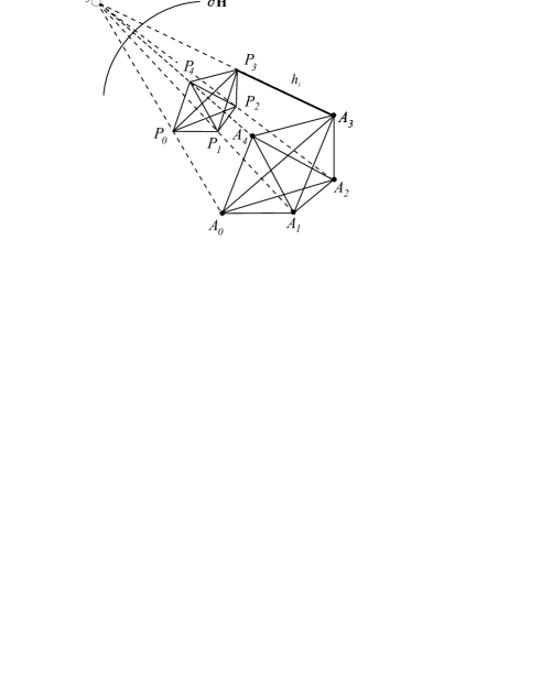
Figure 3:

Let $B_{0},\leavevmode\nobreak\ B_{1},\leavevmode\nobreak\ B_{2},\leavevmode\nobreak\ B_{3},B_{4}$ be the corresponding points of the other cover-polytop of the regular 5-prism. The midpoints of the edges which do not lie in the cover-polytops form a hyperplane denoted by $\pi$. The foot points $P_{i}\leavevmode\nobreak\ (i\in\{0,1,2,3,4\})$ of the perpendiculars dropped from the points $A_{i}$ on the plane $\pi$ form in both cases the same characteristic (or fundamental) simplex $\mathcal{S_{\pi}}$ with Coxeter-Schläfli symbol $[5,3,3,3]$ (see Fig. 3).

Remark 3.1

In $\mathbf{H}^{3}$ (see [13]) the corresponding prisms are called regular $p$-gonal prisms $(p\geq 3)$ in which the regular polyhedra (the cover-faces) are regular $p$-gons, and the side-faces are rectangles. Fig. 4 shows a part of such a prism where $A_{2}$ is the centre of a regular $p$-gonal face, $A_{1}$ is a midpoint of a side of this face, and $A_{0}$ is one vertex (end) of that side. Let $B_{0},\leavevmode\nobreak\ B_{1},\leavevmode\nobreak\ B_{2}$ be the corresponding points of the other $p$-gonal face of the prism.

Analogously to the 3-dimensional case, it can be seen that $\mathcal{S}_{i}=A_{0}A_{1}A_{2}A_{3}$ $A_{4}A_{5}$ $P_{0}P_{1}P_{2}P_{3}P_{4}P_{5}$ $(i=0,2)$ is an complete orthoscheme with degree $d=1$ where $A_{5}$ is an outer vertex of $\mathbf{H}^{5}$ and the points $P_{0},P_{1},P_{2},P_{3},P_{4}$ lie in its polar hyperplane $\pi$ (see Fig. 3). The corresponding regular prism $\mathcal{P}_{i}$ can be derived by reflections in facets of $\mathcal{S}_{i}$ containing the point $A_{3}$.

We consider the images of $\mathcal{P}_{i}$ under reflections in its side facets (side prisms). The union of these 5-dimensional regular prisms (having the common $\pi$ hyperplane) forms an infinite polyhedron denoted by $\mathcal{F}_{i}$.

From the definitions of the prism tilings and the complete orthoschemes of degree $d=1$ follows that a regular prism tiling exists in the $n$-dimensional hyperbolic space $\mathbf{H}^{n},\ \ n\geq 3$ if and only if exists a complete Coxeter orthoscheme of degree $d=1$ with two divergent faces.

The complete Coxeter orthoschemes were classified by Im Hof [5] and [6] by generalizing the method of Coxeter and Böhm appropriately. He showed that they exist only for dimensions $\leq 9$.

On the other hand, if a 5-dimensional regular prism tiling $[p,q,r,s,t]$ exists, then it has to satisfy the following two requirements:

1. The orthogonal projection of the cover-polytop on the hyperbolic hyperplane $\pi$ is a regular Coxeter honeycomb with proper vertices and centres. Using the classical notation of the tesselations, these honeycombs are given by their Coxeter-Schläfli symbols $[p,q,r,s]$.

2. The vertex figures about a vertex of such a prism tiling has to form a 5-dimensional regular polyhedron.

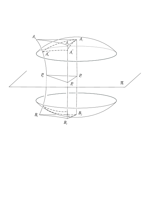
Figure 4:

3.2 The volumes of the orthoschemes

A plane orthoscheme is a right-angled triangle, whose area formula can be expressed by the well known defect formula. For three-dimensional spherical orthoschemes, L. Schläfli about 1850 was able to find the volume differentials depending on differential of the not fixed 3 dihedral angles. Already in 1836, N. I. Lobachevsky found a volume formula for three-dimensional hyperbolic orthoschemes $\mathcal{S}$ [1].

The integration method for orthoschemes of dimension three was generalized by Böhm in 1962 [1] to spaces of constant nonvanishing curvature of arbitrary dimension.

R. Kellerhals in [7] derived a volume formula in the 3 dimensional hyperbolic space for the complete orthoschemes of degree $d,\leavevmode\nobreak\ (d=0,\leavevmode\nobreak\ 1,\leavevmode\nobreak\ 2)$ and she explicitly determined in [8] the volumes of all complete hyperbolic orthoschemes in even dimension ($n\geq 4$), moreover, she in [10] developed a procedure to determine the volumes of 5-dimensionalal hyperbolic orthschemes.

The volumes of the complete orthoschemes $\mathcal{S}_{i}$ $(i=0,2)$ of $d=1$ can be computed by volume differential formula of L.  Schläfli with the the following formula (see [4]):

$$Vol_{5}(\mathcal{S}_{i})=\frac{1}{4}\int_{\alpha_{i}}^{\frac{2\pi}{5}}{Vol_{3}([5,3,\beta(t)])dt+\frac{\zeta(3)}{3200}}$$ (3.1)

with a compact tetrahedron $[5,3,\beta(t)]$ whose angle parameter $0<\beta(t)<\frac{\pi}{2}$ is given by

$$\beta({t})=\arctan{\sqrt{2-\cot^{2}{t}}}.$$

Then, the volume of the 3-dimensional orthoscheme face $[5,3,\beta(t)]$ as given by Lobachevsky’s formula:

$$\begin{gathered}Vol_{3}([5,3,\beta(t)])=\frac{1}{4}\{\mathcal{L}_{2}\big{(}\frac{\pi}{5}+\theta(t)\big{)}-\mathcal{L}_{2}\big{(}\frac{\pi}{5}-\theta(t)\big{)}-\mathcal{L}_{2}\big{(}\frac{\pi}{6}+\theta(t)\big{)}+\\ \mathcal{L}_{2}\big{(}\frac{\pi}{6}-\theta(t)\big{)}+\mathcal{L}_{2}\big{(}\beta(t)+\theta(t)\big{)}-\mathcal{L}_{2}\big{(}\beta(t)-\theta(t)\big{)}+2\mathcal{L}_{2}\big{(}\frac{\pi}{2}-\theta(t)\big{)}\end{gathered}$$ (3.2)

where

$$\mathcal{L}(\omega)=-\int_{0}^{\omega}{\log|2\sin{t}|dt},\ \omega\in\mathbf{R},$$

is the Lobachevsky’s function and

$$\theta(t)=\arctan\frac{\sqrt{1-4\sin^{2}\frac{\pi}{5}\sin^{2}{\beta(t)}}}{2\cos\frac{\pi}{5}\cos\beta(t)}.$$

3.3 The optimal hyperball packing

The equidistance surface (or hypersphere) is a quadratic surface at a constant distance from a plane in both halfspaces. The infinite body of the hypersphere is called hyperball.

The 5-dimensional hypersphere with distance $h$ to a hyperplane $\pi$ is denoted by $\mathcal{H}^{h}$. The volume of a bounded hyperball piece $\mathcal{H}^{h}(\mathcal{A})$ delimited by the 4-polytop $\mathcal{A}\subset\pi$, $\mathcal{H}^{h}$ and some to $\pi$ orthogonal hyperplanes derived by the facets of $\mathcal{A}$ can be determined by the formula (3.3) that follows by the generalization of the classical method of J. Bolyai:

$$Vol({\mathcal{H}}^{h}(\mathcal{A}))=\frac{1}{16}Vol(\mathcal{A})k\Big{(}\frac{1}{2}\sinh\frac{4h}{k}+4\sinh\frac{2h}{k}\Big{)}+\frac{3hVol(\mathcal{A})}{8},$$ (3.3)

where the volume of the hyperbolic 4-polytop $\mathcal{A}$ lying in the plane $\pi$ is $Vol(\mathcal{A})$. The constant $k=\sqrt{\frac{-1}{K}}$ is the natural length unit in $\mathbf{H}^{n}$. $K$ will be the constant negative sectional curvature.

We are looking for the optimal hyperball $\mathcal{H}^{h_{i}}_{opt}$ inscribed in $\mathcal{T}_{i}$ with maximal height.

The optimal hypersphere $\mathcal{H}_{opt}^{h_{i}}$ touches the cover-faces of the regular 5-prisms containing by $\mathcal{F}_{i}$. Therefore, the optimal distance from the 4-midplane $\pi$ will be $h_{i}=P_{4}A_{4}$ (Fig. 3).

We consider one from the former defined 5-dimensional regular prism tilings $\mathcal{T}_{i}$ $(i=0,2)$ and the infinite polyhedron $\mathcal{F}_{i}$ derived from that (the union of 5-dimensional regular prisms having the common hyperplane $\pi$). $\mathcal{F}_{i}$ and its images under reflections in its ”cover facets” fill the hyperbolic space $\mathbf{H}^{5}$ without overlap thus we obtain by the above images of $\mathcal{H}_{opt}^{h_{i}}$ a locally optimal hyperball packing to the tiling $\mathcal{T}_{i}$ $(i=0,2)$.

The points $P_{4}({\mathbf{p}}_{4})$ and $A_{4}({\mathbf{a}}_{4})$ are proper points of the hyperbolic 5-space and $P_{4}$ lies on the polar hyperplane $pol(A_{5})$ of the outer point $A_{5}$ thus

$$\begin{gathered}\mathbf{p}_{4}=c\cdot\mathbf{a}_{5}+\mathbf{a}_{4}\in\mbox{\boldmath$a$}^{5}\Leftrightarrow c\cdot\mathbf{a}_{5}\mbox{\boldmath$a$}^{5}+\mathbf{a}_{4}\mbox{\boldmath$a$}^{5}=0\Leftrightarrow c=-\frac{\mathbf{a}_{4}\mbox{\boldmath$a$}^{5}}{\mathbf{a}_{5}\mbox{\boldmath$a$}^{5}}\Leftrightarrow\\ \mathbf{p}_{4}\sim-\frac{\mathbf{a}_{4}\mbox{\boldmath$a$}^{5}}{\mathbf{a}_{5}\mbox{\boldmath$a$}^{5}}\mathbf{a}_{5}+\mathbf{a}_{4}\sim\mathbf{a}_{4}(\mathbf{a}_{5}\mbox{\boldmath$a$}^{5})-\mathbf{a}_{5}(\mathbf{a}_{4}\mbox{\boldmath$a$}^{5})=\mathbf{a}_{4}h_{55}-\mathbf{a}_{5}h_{45},\end{gathered}$$ (3.4)

where $h_{ij}$ is the inverse of the Coxeter-Schläfli matrix $c^{ij}$ (see (2.5)) of the orthoscheme $\mathcal{S}_{i}$. The hyperbolic distance $h_{i}$ can be calculated by the following formula [11]:

$$\begin{gathered}\cosh{P_{4}A_{4}}=\cosh{h_{i}}=\frac{-\langle{\mathbf{p}}_{4},{\mathbf{a}}_{4}\rangle}{\sqrt{\langle{\mathbf{p}}_{4},{\mathbf{p}}_{4}\rangle\langle{\mathbf{a}}_{4},{\mathbf{a}}_{4}\rangle}}=\\ =\frac{h_{45}^{2}-h_{44}h_{55}}{\sqrt{h_{44}\langle\mathbf{p}_{4},\mathbf{p}_{4}\rangle}}=\sqrt{\frac{h_{44}\leavevmode\nobreak\ h_{55}-h_{45}^{2}}{h_{44}\leavevmode\nobreak\ h_{55}}}.\end{gathered}$$

The volume of the polyhedron $\mathcal{S}_{i}$ is denoted by $Vol_{5}(\mathcal{S}_{i})$ (see Section 2).

For the density of the packing it is sufficient to relate the volume of the optimal hyperball piece to that of its containing polyhedron $\mathcal{S}_{i}$ (see Fig. 3) because the tiling can be constructed of such polyhedron. This polytope and its images in $\mathcal{F}_{i}$ divide the $\mathcal{H}^{h_{i}}$ into congruent pieces whose volume is denoted by $Vol({\mathcal{H}_{opt}^{h_{i}}})$. We illustrate in the 3-dimensional case such a hyperball piece $A_{2}A_{0}^{\prime}A_{1}^{\prime}P_{0}P_{1}P_{2}$ in Fig. 4.

The density of the optimal hyperball packing to the prism tiling $\mathcal{T}_{i}$ $(i=0,2)$ is defined by the following formula:

Definition 3.1

$$\delta^{opt}(\mathcal{T}_{i}):=\frac{Vol(\mathcal{H}_{opt}^{h_{i}})}{Vol_{5}({\mathcal{S}_{i}})}.$$ (3.6)

$\delta^{opt}(\mathcal{T}_{i})$ can be determined by the formulas (3.1), (3.2), (3.3) and (3.5) using, that the volume $Vol(\mathcal{A})=Vol(\mathcal{S}_{\pi})$ (see (3.3)) of the 4-dimensional polytope $\mathcal{S}_{\pi}$ with Coxeter symbol $[5,3,3,3]$ in both cases is

$$Vol(\mathcal{S}_{\pi})=\frac{\pi^{2}}{10800}\approx 0.00091385.$$

Finally we get the following results:

Table 1   $\varSigma_{53333}$ $\varSigma_{53334}$   $Vol(S_{i})$ $\approx 0.00076730$ $\approx 0.00198469$   $h_{i}$ $\approx 0.38359861$ $\approx 0.53063753$   $Vol(\mathcal{H}^{h_{i}}_{opt})$ $\approx 0.00038760$ $\approx 0.00059001$   $\delta^{opt}$ $\approx 0.50514481$ $\approx 0.29727979$

Remark 3.2

The optimal density of the Coxeter tiling $\mathcal{T}_{1}$ with Coxeter symbol $[5,3,3,3,3^{1,1}]$ is equal to $\delta^{opt}(\mathcal{T}_{0})\approx 0.50514481$.

The next conjecture for the optimal hyperball packings can be formulated.

Conjecture 3.1

The above described optimal hyperball packings to Coxeter tilings $[5,3,3,3,3]$ and $[5,3,3,3,3^{1,1}]$ provide the densest hyperball packings in the 5-dimensional hyperbolic space $\mathbf{H}^{5}$.

Remark 3.3

Regular hyperbolic honeycombs exist only up to 5 dimensions [3]. Therefore regular prism tilings can exist up to 6 dimensions. From the definitions of the prism tilings and the complete orthoschemes of degree $d=1$ it follows that prism tilings exist in the $n$-dimensional hyperbolic space $\mathbb{H}^{n},\ \ n\geq 3$ if and only if there exist complete Coxeter orthoschemes of degree $d=1$ with two divergent faces. From the paper [6] it follows that in the 5-dimensional hyperbolic space there is a further type and in the 6-dimensional hyperbolic space there is no such a Coxeter orthoschem.

Jenő Szirmai,   Budapest University of Technology and
Economics, Institute of Mathematics, Department of Geometry
H-1521 Budapest, Hungary
Email:   szirmai@math.bme.hu,  www.math.bme.hu /$\sim$szirmai

References

- [1] Böhm,J.-Hertel,E. Polyedergeometrie in -dimensionalen Räumen konstanter Krümmung, Birkhäuser, Basel (1981).
- [2] Belolipetsky, M.-Emery, V. On volumes of arithmetic quotients of , odd, Proc. Lond. Math. Soc., (to appear), preprint arXiv:1001.4670.
- [3] Coxeter, H. S. M. Regular honeycombs in hyperbolic space, Proceedings of the international Congress of Mathematicians, Amsterdam, (1954) III , 155–169.
- [4] Emery, V.-Kellerhals, R. The three smallest compact arithmetic hyperbolic 5-orbifolds, Algebr. Geom. Topol., (2013) 13 , 817–829.
- [5] Im Hof, H.-C. A class of hyperbolic Coxeter groups, Expo. Math., (1985) 3 , 179–186.
- [6] Im Hof, H.-C. Napier cycles and hyperbolic Coxeter groups, Bull. Soc. Math. Belgique, (1990) 42 , 523–545.
- [7] Kellerhals, R. On the volume of hyperbolic polyhedra, Math. Ann., (1989) 245 , 541–569.
- [8] Kellerhals, R. The Dilogarithm and Volumes of Hyperbolic Polytopes, AMS Mathematical Surveys and Monographs, (1991) 37, 301–336.
- [9] Kellerhals, R. Ball packings in spaces of constant curvature and the simplicial density function, Journal für reine und angewandte Mathematik, (1998) 494 , 189–203.
- [10] Kellerhals, R. Volumes of hyperbolic 5-orthoschemes and the trilogarithm, Comment. Math. Helv., (1992) 67 , 648–663.
- [11] Molnár, E. Projective metrics and hyperbolic volume, Annales Univ. Sci. Sect. Math., (1989) 4/1, 127–157.
- [12] Molnár, E. The projective interpretation of the eight 3-dimensional homogeneous geometries, Beitr. Algebra Geom., (1997) 38/2, 261–288.
- [13] Szirmai, J. The -gonal prism tilings and their optimal hypersphere packings in the hyperbolic 3-space, Acta Math. Hungar. (2006) 111 (1-2), 65–76.
- [14] Szirmai, J. The regular prism tilings and their optimal hyperball packings in the hyperbolic -space, Publ. Math. Debrecen (2006) 69 (1-2), 195–207.
- [15] Vermes, I. Über die Parkettierungsmöglichkeit des dreidimensionalen hyperbolischen Raumes durch kongruente Polyeder, Studia Sci. Math. Hungar. (1972) 7, 267–278.
- [16] Vermes, I. Bemerkungen zum Parkettierungsproblem des hyperbolischen Raumes, Period. Math. Hungar. (1973) 4, 107–115.
- [17] Vermes, I. Ausfüllungen der hyperbolischen Ebene durch kongruente Hyperzykelbereiche, Raumes, Period. Math. Hungar. (1979) 10/4, 217–229.