Melting behavior and different bound states in three stranded DNA models

Abstract

Thermal denaturation of DNA is often studied with coarse-grained models in which native sequential base pairing is mimicked by the existence of attractive interactions only between monomers at the same position along strands (Poland and Scheraga models). Within this framework, the existence of a three strand DNA bound state in conditions where a duplex DNA would be in the denaturated state was recently predicted from a study of three directed polymer models on simplified hierarchical lattices ($d>2$) and in $1+1$ dimensions. Such phenomenon which is similar to the Efimov effect in nuclear physics was named Efimov-DNA. In this paper we study the melting of the three-stranded DNA on a Sierpinski gasket of dimensions $d<2$ by assigning extra weight factors to fork openings and closings, to induce a two-strand DNA melting. In such a context we can find again the existence of the Efimov-DNA-like state but quite surprisingly we discover also the presence of a different phase, to be called a mixed state, where the strands are pair-wise bound but without three chain contacts. Whereas the Efimov DNA turns out to be a crossover near melting, the mixed phase is a thermodynamic phase.

I INTRODUCTION

A loosely bound state of a triple stranded DNA when no two are bound was recently found with a theoretical approach and named Efimov-DNA efidna ; zeros ; tanlim . It occurs at and above the melting point of a double stranded DNA (dsDNA) melt ; unzip1 ; unzip2 ; unzip3 ; kapri , and is reminiscent of the Efimov effect in quantum mechanics efimov1 ; efimov2 . In fact, the sequential base pairing of a DNA opens up a path to make a formal connection between a quantum problem and the DNA thermodynamics, with thermal fluctuations playing the role of quantum fluctuations. Owing to this quantum analogy, an Efimov-DNA could be an affordable system in the domain of classical biology for studying aspects of the quantum Efimov physics. In this paper we widen the scope of the Efimov physics by establishing the presence of the effect in certain classes of low-dimensional DNA models by staying purely in the classical domain of statistical mechanics. We also show that the same cause that produces the Efimov-like effect in DNA can lead to a new phase in triple-stranded DNA, a phase we call a mixed phase.

In 1970, a novel phenomena in quantum mechanics, the Efimov effect efimov1 ; efimov2 , was discovered, which resembled the by-then-forgotten Thomas effect of 1930’s thomas . Three nucleons with a critical short range pair potential become bound due to an emergence of a long range interaction. The result was a tower of an infinite number of bound states right at the critical threshold of the two-body binding. As one moves away from the critical point the number of bound states decreases and vanishes at a particular strength. This three-body bound state has a size much larger than the range of the short range pair potential. Such a loose three-body bound state is named as the quantum Efimov state.

The paths of particles in quantum mechanics (QM), in the path integral formalism, are analogous to Gaussian polymers under an imaginary time transformation; the time of quantum mechanics maps on to the contour length of the polymers. In QM, along the paths of two interacting particles, the interactions are strictly at the same time only. This maps nicely onto the sequential base pairing of a dsDNA. The excursions of the quantum particles in the classically forbidden region because of quantum fluctuations correspond to the bubbles on a DNA generated by thermal fluctuations. The infinite time limit in QM corresponds to an infinitely long DNA, a necessity for a phase transition. For the case of base pairing as the only form of mutual interaction, the melting is equivalent to the unbinding transition of a pair of particles in quantum mechanics when the bound state energy approaches zero by tuning the potential. This basic connection prompts the similarities between the Efimov problem in QM and a tsDNA.

Triple-stranded DNA (tsDNA) is well-known in biology rich57 ; buske . The base sequence of a double stranded DNA (dsDNA) allows a third strand to bind via the Hoogsteen or the reverse Hoogsteen pairing to form a triple helix frank95 ; radha . There are evidences, from NMR, of Hoogsteen pairing formed dynamically (1% of time) even in a normal DNA JACS2012 . The triplex helix can also be formed with DNA-RNA Roberts and DNA-peptide nucleic acid (PNA), whose uncharged peptide backbone helps in the stabilization of the triplet structure Nielsen ; ray00 ; sun96 ; Betts . A triple helix formation controls the gene expression, which may be of use in antibiotics antibio , and therapeutic applications like targeting a specific sequence in gene therapy therapy1 ; therapy2 ; helen . All of these involve tightly bound states of a size determined by the hydrogen bond length. The Efimov-DNA however is not a tight bound state like these triple helices and one does not need any special pairing for its formation.

The nature of dsDNA melting depends on many factors and could either be an all-or-none process or be mediated by the formation of bubbles along the chain. Bubble formations increase the entropy of the bound state. The melting takes place when the gain in entropy by strand unbinding outweighs the energy gain of the bound state. At or close to the duplex melting, if a double stranded DNA allows bubbles of any length, a third strand of DNA can pair with the strands of the bubble. This process, known in biology as the strand exchange mechanism, would lead to a bound state of the three together. The possibility of a long-range attraction, an important aspect of the Efimov effect, has been argued by a polymeric scaling analysis in Ref. efidna . The existence of a three-strand bound state has further been verified by real space renormalization group (RG) on hierarchical lattices of dimensions $d>2$, transfer matrix calculations in real space in $1+1$ dimensions, and by an RG limit cycle for polymer models in continuum in $3$ dimensions efidna ; zeros ; tanlim .

Figure 1: Schematic diagram showing the predicted phases as temperature $T$ is varied. While the Efimov-DNA is not a phase, mixed phase is predicted to be a thermodynamic phase. A triplex DNA crosses over to the Efimov-DNA before melting at $T_{t}$, while in the case of a mixed phase, there will be a two-step melting, a triplex-to-mixed transition at $T_{t}$, and a mixed-to-denatured DNA transition at $T_{c}$.

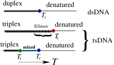
The triplex formed by the pairwise attraction of bases has a melting point higher than the duplex melting temperature. As already mentioned, the Efimov-DNA occurs in the region between the melting point of dsDNA and tsDNA. This is an exotic state mainly because of the special role played by the third strand, but thermodynamically it is not a distinct phase. It is a continuation of the low temperature triplex bound state. This raises an interesting issue whether the Efimov like state mediated by the third strand of DNA can be stabilized as a thermodynamic phase, distinct from the triplex and the denatured state. This mixed phase, alluded to at the beginning, is a bound state where, in any stretch of length, one strand remains unbound with two others paired; it should share a boundary with the denatured DNA on the high temperature side and a boundary with the triplex state on the low temperature side. We establish in this paper that such a mixed phase does occur if the bubble formation on the DNA is controlled suitably. The major consequence of this intermediate mixed phase is that a tsDNA would undergo two phase transitions, triplex$\leftrightarrow$mixed$\leftrightarrow$denatured, as opposed to a simple melting. See Fig. reffig:newx. This is one of the important results of this paper.

It may now be asked, what it is that is responsible for the Efimov effect. For a broader perspective, it helps to define the DNA melting problem in any dimension, like in many other polymer problems. On one hand, the standard quantum mechanical results and the polymeric scaling argument indicate the importance of large scale fluctuations in bubbles to produce an effective inverse square law attraction efimov1 ; efidna . On the other hand, the models of DNA on hierarchical lattices ($d>2$), which do not have any metric, also show the Efimov-DNA. It is then tempting to hypothesize that the Efimov effect of three being bound but no two, is a consequence of a phase transition through its associated non-analytic behaviour. If true, this would broaden the range of situations where the Efimov effect could be seen. Admittedly, it is difficult to establish the hypothesis in the quantum domain but it can be done in the DNA context. For example, in lower dimensions ($d\leq 2$), the bubble entropy is not enough to cause a melting, so that DNA would remain bound at all temperatures for any arbitrarily weak short-range attraction comment . However, for a DNA in a lower dimension $d\leq 2$, a phase transition can be triggered by adding extra factors. These extra factors are either local constraints in bubble opening (e.g. crossing) or the hard core repulsion or some cooperativity weight factors ($\sigma$) for each bubble formed in the model between the DNA strands. A test of the hypothesis would then be to show the existence of an Efimov-DNA in such low dimensional models with phase transitions.

In this paper we aim to verify the robustness of such a finding and to reach such a purpose we want to investigate the effects of variation of the $\sigma$ parameter. Hence it is worthwhile to consider a model in a lower dimensional lattice which is amenable to exact treatments and where $\sigma$ the cooperative parameter can be easily tuned. This lattice turns out to be the Sierpinski gasket, the common regular fractal which have been widely used in studying different statistical models, for instance the Ising model, the directed or the self avoiding polymer model, the Potts model, the sandpile model, the ice-type vertex models, models of polymers under a force dhar ; sgflavio ; yash ; critpheno ; knez ; elez ; ice . It is remarkable that very often the results obtained on Sierpinski gasket or on other hierarchical lattices turn out to be true in the real world, for instance, the collapse transition ($\theta$) point for linear polymer dharvan ; OSST91 or, as we will show later in the paper, the correct order (first) of the denaturation transition of double-stranded DNA.

II Outline

This paper is organized as follows. In Sec. III, our model on a Sierpinski gasket is introduced. In Secs. IV and V two- and three-polymer problems on a fractal lattice are introduced. The exact recursion relations of the partition functions for both the crossing and the noncrossing cases are written and the method of calculations is discussed. The two-chain phase diagrams are discussed. With various interactions and the crossing or the noncrossing conditions three different models of the three-chain system are introduced. Results obtained from the exact recursion relations are discussed in Secs. VI and VII.

III model

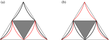
A Sierpinski gasket is a fractal lattice obtained after an infinite iteration from a single equilateral triangular lattice. This particular lattice is drawn on the two dimensional ($d=2$) plane. Taking out the middle piece of a triangle yields three smaller triangles and, by repeating this for every allowed triangle, the fractal lattice is formed recursively; see Fig. 2. The dimension for an infinite lattice is

$$d=\frac{\ln N_{n}}{\ln L_{n}}=\frac{\ln 3}{\ln 2}\approx 1.58,$$ (1)

where $N_{n}$ is the number of the surviving triangles and $L_{n}$ is the number of bonds of the lattice along any one side of the lattice at the $n$th generation.

Figure 2: Recursive construction of the Sierpinski gasket.

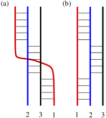
In order to mimic the Poland-Scheraga PS66 DNA-like models in which monomers in different strands interact only if their position along the chain is the same (complementary bases), we consider directed polymers on a Sierpinski gasket which are restricted to occupy only the nonhorizontal bonds as shown in Fig. 3. In such a way, each time two different strands occupy the same bond, it is automatically guaranteed that they share the same chemical distance from the origin. Still, there can be two different classes of models differing in the restrictions on the crossing of the two strands. Two configurations with a bubble are shown for generation $n=1$ in Figs. 3(a) and 3(b). If we allow crossing, the strands can exchange and both Figs. 3(a) and 3(b) are allowed. In the noncrossing case, only (a) is allowed. The crossing among the polymers increases the number of configurations, resulting in more entropic contributions compared to the noncrossing case.

Figure 3: A polymer is not allowed on any horizontal bond. In the figure, two possible configurations of two polymers (black (dark) and red (light)) are shown ($b_{n}$ and $g_{n}$ type from Fig. 4). The crossing case allows both while only (a) is allowed for the noncrossing case.

In this approach the sequence of bases is not explicitly considered since the model is coarse grained in character. In this respect each monomer is not to be thought of as a single base, but as a group of bases (block). Consequently a mismatch between corresponding blocks has to be very disfavored with respect to a correct matching.

We can consider two or three different polymers. The following weights are assigned to them:

• Fugacity $z$ for each bond,

• Boltzmann factor $y_{ij}=e^{\beta\epsilon_{ij}}$, when a single bond is shared by the two polymers $i$ and $j$ with binding energy $\epsilon_{ij}$, and $y_{ijk}=e^{\beta\epsilon_{ijk}}$ when a single bond is shared by the three polymers with the binding energy $\epsilon_{ijk}$. Here $\beta$ represents the inverse temperature $T$, $\beta=1/k_{\rm B}T$, where $k_{\rm B}$ is the Boltzmann constant.

• $\sigma_{ij}$ for the two-chain and $\sigma_{ijk}$ for the three-chain bubble opening or closure.

The weight of a walk of a single chain of length $N$ is $z^{N}$, where $N$ is the number of bonds. Usually dhar ; OSST91 ; dharsingh one can consider $z$ as an extra variable, the fugacity for the length of the polymers in a grand-canonical ensemble, but here we will set it to $1$, as is discussed below. We use $z$ when a direct computation of the free energy is required.

There are two special values of $\sigma$; $\sigma=1$ implies that no weight is given for bubble opening or closure, and $\sigma=0$ implies no bubble formation, i. e., a model without any bubble (fork model). In biological contexts the co-operativity factors $\sigma$’s depend, for example, on the chain length, the ionic strength, the stacking potential, etc. ionic . Most of the studies have reported the value of cooperativity factor in the range $10^{-4}$–$10^{-5}$ with the loop nucleation free energy as $\sim-k_{B}T\ln\sigma\sim 10k_{B}T$. We shall take the cooperativity factor as a controlling parameter, not necessarily restricted to small values.

To study the melting of DNA on a fractal lattice, we need to define the partition functions for the two- and the three-chain systems as shown in Fig. 4. We choose $z=1$ to be in the canonical ensemble. The standard way to study the polymers on a fractal lattice is to find out the fixed point of $z$ by an RG procedure as proposed by Dhar dhar . This corresponds to the grand canonical ensemble, where the fixed point of $z$ gives the free energy. We know that the choice of ensemble does not matter, as long as we work with the large lengths of the polymers. In our approach we calculate the free energies of different possible phases in the canonical ensemble, look for the most favorable one, and obtain the phase diagram directly from the free energies. Since all the polymers are of same length ($N=2^{n+1}\to\infty$) and traverse the whole lattice, we may set $z=1$.

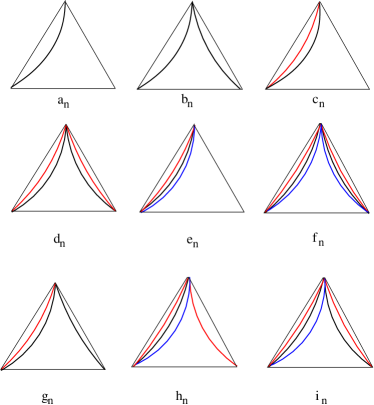
Different possible polymer configurations are shown in Fig. 4. The corresponding partition functions $a_{n}$, $b_{n}$, $c_{n}$, $d_{n}$, $e_{n}$, $f_{n}$, $g_{n}$, $h_{n}$, $i_{n}$ are defined at the $n$th generation and their corresponding recursion relations can be easily computed for successive generations. An example of the procedure to obtain the recursion relation is given in Appendix A. The initial conditions (the partition functions at the first stage of iteration) are dictated from the physical properties of the studied model.

Figure 4: The partition functions for two and three strands irrespective of crossing conditions of the chains.

IV Two stranded DNA on the Gasket

In order to explain our strategy and to fix some preliminary results let us first consider the melting of a double stranded DNA. The partition functions of a single chain and a double chain for the $n$th generation are given by $b_{n}$ and $d_{n}$ respectively. However, to do the sum over all configurations, one needs the sub-partition functions, $a_{n},c_{n}$ and $g_{n}$ as one sees from Fig. 3 and Appendix A. The crossing and the noncrossing cases are discussed separately below.

IV.1 With crossing

We first consider a two-chain system where the walks can cross each other. Here $y$ is the weight at the bond for sharing it by the two polymers. The two-chain bubble opening or closure is associated with the weight $\sigma$ at the vertex. Five partition functions are necessary and using the label used in Fig. 4 their values for the $(n+1)$th generation are given by (see Appendix A)

$$a_{n+1} =a_{n}^{2},$$ (2a)

$$b_{n+1} =b_{n}^{2}+a_{n}^{2}b_{n},$$ (2b)

$$c_{n+1} =c_{n}^{2},$$ (2c)

$$d_{n+1} =d_{n}^{2}+2g_{n}^{2}b_{n}+c_{n}^{2}d_{n},$$ (2d)

$$g_{n+1} =a_{n}g_{n}(b_{n}+c_{n}).$$ (2e)

The Boltzmann factors and other weights are defined on the bonds and the sites. They are therefore specified for the smallest triangle, i.e., at the zeroth generation. Those specifications act as the initial conditions for the recursion relations. The initial conditions are taken as

$$a_{0}=1,~{}b_{0}=1,~{}c_{0}=y,~{}d_{0}=y^{2},~{}g_{0}=y\sigma.$$ (3)

These values follow from Fig. 4 by counting the shared bonds and bubble opening or closing. For $c_{0}$ and $g_{0}$ there is only one bond with two strands on it and hence they require a Boltzmann factor $y$. On the other hand, $d_{n}$ has two shared bonds, thereby requiring a factor $y^{2}$. A configuration like $g_{n}$ is required to open or close a bubble. Hence $g_{n}$ involves an additional $\sigma$ for the junction point.

By iterating the equations it turns out that the leading terms are coming from the generating function $b_{n}$ (single chain) and $d_{n}$ (two chains). It is then convenient to look at the ratio

$$r_{1}=\frac{d_{n+1}}{b_{n+1}^{2}}.$$ (4)

Figure 5: The two-chain phase diagram for $\sigma$ vs $y$. (a) The polymers can cross each other, (b) the noncrossing case. For both the cases, the two-chain melting is at $y_{c}(0)=1.264...$ for $\sigma=0$. Here and elsewhere, $y=1$ ($y=\infty$) corresponds to infinite (zero) temperature.

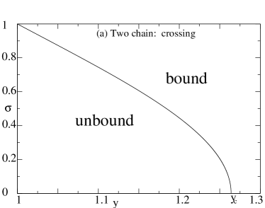
This ratio compares the two-chain bound state free energy with the free energy when the two strands are in the denatured state. By monitoring the divergence or the convergence of $r_{1}$, for given values of $\sigma$ and $y$, one can easily and quickly pinpoint the denaturation transition and obtain the phase diagram in the $y$-$\sigma$ plane. The phase diagram is shown in Fig. 5. The transition is from the unbound to the bound state of the two-stranded DNA at $y=y_{c}(\sigma)$.

For $\sigma=0$, there are no bubbles. In this situation, the bound state partition function for the $n$th generation consists of two factors, the Boltzmann factor and the number of configurations of the bound pair $b_{n}$, i.e.

$$d_{n}=b_{n}\;y^{N},\quad N=2^{n+1},$$ (5)

while the partition function of the unbound state is $b_{n}^{2}$. The continuity of the free energy at the transition point ($r_{1}=1$) then gives the transition point as

$$\ln y_{c}(0) = \lim_{n\to\infty}\frac{1}{2^{n+1}}\ \ln b_{n},$$

$${\rm or,}\quad y_{c}(0) = 1.2640847353....$$ (6)

This value corresponds to the temperature at which the binding energy per bond $\epsilon$ is equal to the entropic free energy ($Ts$) of a single chain, viz.,

$$T_{c}=\epsilon/s,\quad{\rm with}\ s=\lim_{n\to\infty}(1/N)\ln b_{n}.$$ (7)

IV.2 No crossing

If the crossing between the two strands DNA is not allowed, the recursion relations are same as the crossing case except for $d_{n}$, which in this case is

$$d_{n+1}=d_{n}^{2}+g_{n}^{2}b_{n}+c_{n}^{2}d_{n}.$$ (8)

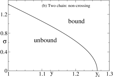
The initial conditions are still given by Eq. (3). A similar comparison method [Eq. (4)] is used here as in the two-chain crossing case. We obtain the phase diagram in the $y$-$\sigma$ plane as shown in Fig. 5(b). For $\sigma=0$ the two-chain melting is at $y_{c}(0)=1.264...$, which is the same as in the crossing case. There is a difference between the crossing and the noncrossing melting curve for $\sigma\neq 0$. In fact, the two curves can be mapped onto one another by rescaling $\sigma$ by $1/\sqrt{2}$ in the crossing case; indeed, the consequent rescaling of $g_{n}$ necessary to keep the initial condition in the form of (3) allows us to change Eq. (8) into Eq. (2d). In particular it can be noticed that for $\sigma=1$ the melting transition occurs at a finite temperature only for the noncrossing model. For the crossing case, $y_{c}(\sigma=1)=1$, but for the noncrossing case $y_{c}(\sigma=\sqrt{2})=1$.

It is important to notice that for both the considered models (with crossing and no crossing) and for any $\sigma$ , the first derivative of the free energy is discontinuous at the thermal transition (see Fig. 11). Therefore, despite its simplicity, our model predicts a first order transition for DNA denaturation as observed experimentally Kafri .

V Three strands

When we consider the three-chain system, several cases are possible. With the crossing and the noncrossing conditions and the choices of the interacting and the noninteracting pairs, we classify different models. Among the many possible varieties we will discuss only three of them, TS1, TS2, and TS3 since they exhibit the full range of critical behaviours we explored. The models are the following:

1. Model TS1: This is the noncrossing case with a weight for two-chain bubble opening or closure of all pairs. The weight is penalizing bubbles for $\sigma<1$ but favoring for $\sigma>1$. There is no contact energy between chains $1$ and $3$. These two chains are nevertheless coupled with each other through the $\sigma$ weight, only when all the three strands are bound together. As a consequence, the opening or closure in the triplex state is weighted twice (it involves two pairs) with respect to the duplex state.

2. Model TS2: This is the crossing case with the three-chain repulsion, so that the overall energy of the triplex state is the same as for the duplex state. Similar to TS1, the weight for a two-chain bubble opening or closure is present for all pairs, so that the opening or the closure in the triplex state is weighted twice with respect to the duplex state.

3. Model TS3: This is the crossing case with the three-chain repulsion and a weight for both the two- (for all pairs) and the three-chain bubble opening or closure. The weight for the three-chain bubbles counters that for two-chain ones, so that both the overall energy and the weight for the opening or closure are the same in the triplex and in the duplex state.

V.1 Model TS1: Noncrossing

In this case walks can not cross each other. We assign a weight Boltzmann factor $y$ for each interaction between chains 1 and 2, and 2 and 3 i. e., $y_{12}=y_{23}=y$, but no interaction between chains 1 and 3, i. e., $y_{31}=1$. The weight $\sigma$ is assigned for each bubble opening between all pairs, i. e., $\sigma_{12}=\sigma_{23}=\sigma_{31}=\sigma$. When all chains are together we consider a weight $y^{2}$ and such a situation can also be described if we take $y_{12}=y_{23}=y_{31}=y$ and $y_{ijk}=1/y$. If $y>1$, $y_{ijk}$ is repulsive in nature. The two definitions of the contact energies are equivalent only because of the noncrossing constraint.

Figure 6: Model TS1: The three-chain phase diagram in the $y$–$\sigma$ plane for model TS1. The bound, the unbound, the Efimov, and the mixed states are shown. The solid line is the two-chain melting curve and is valid for the three chain case in the region $y>y_{E}=1.07526...$ but not in the region $y<y_{E}$. The dashed-dotted (green) line is the boundary for the mixed phase while the dashed line is the melting line for the Efimov-DNA.

The recursion relations for the partition functions for this model are given by

$$a_{n+1} =a_{n}^{2},$$ (9a)

$$b_{n+1} =b_{n}^{2}+a_{n}^{2}b_{n},$$ (9b)

$$c_{n+1} =c_{n}^{2},$$ (9c)

$$d_{n+1} =d_{n}^{2}+g_{n}^{2}b_{n}+c_{n}^{2}d_{n},$$ (9d)

$$e_{n+1} =e_{n}^{2},$$ (9e)

$$f_{n+1} =f_{n}^{2}+e_{n}^{2}f_{n}+h_{n}^{2}d_{n}+i_{n}^{2}b_{n},$$ (9f)

$$g_{n+1} =a_{n}g_{n}(b_{n}+c_{n}),$$ (9g)

$$h_{n+1} =h_{n}(a_{n}e_{n}+b_{n}c_{n}),$$ (9h)

$$i_{n+1} =i_{n}(c_{n}e_{n}+d_{n}a_{n})+g_{n}^{2}h_{n},$$ (9i)

with initial conditions:

$$a_{0}=1,b_{0}=1,c_{0}=y,d_{0}=y^{2},e_{0}=y^{2},f_{0}=y^{4},$$

$$g_{0}=y\sigma,h_{0}=y^{2}\sigma^{2},i_{0}=y^{3}\sigma^{2}.$$ (10)

The powers of $y$ follow from Fig. 4 by counting the pairs sharing the bonds. For the $\sigma$ factors, we note that both $h_{0}$ and $i_{0}$ correspond to a single chain breaking off from a triplet, thereby producing two “bubbles” with the remaining two. Hence $\sigma^{2}$ for both these partition functions. For example, in $i_{0}$, one bond with three chains has three pairs requiring $y^{3}$ but with an additional factor $y_{123}=1/y$ for the three chain interaction, while the other bond has only one pair requiring a factor $y$. This gives $y^{3}$ with $\sigma^{2}$ for opening or closing of two bubbles.

We look at the divergence or convergence of the ratios

$$r_{2} = \frac{f_{n+1}}{b_{n+1}^{3}},$$ (11)

$$r_{3} = \frac{f_{n+1}}{b_{n+1}d_{n+1}},$$ (12)

for given $\sigma$ and $y$. The idea behind the choice of the above ratios is to compare the three-chain free energy with the free energy when three chains are free [$r_{2}$ in Eq. (11)], or when one chain remains isolated with the other two forming a duplex [$r_{3}$ in Eq. (12)].

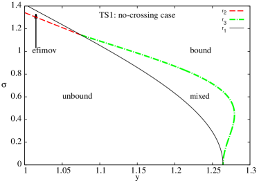
By looking at the divergence or convergence of the ratios $r_{2}$ and $r_{3}$ for different values of $y,~{}\sigma$ and comparing these values with the two-chain melting curve, different phases can be identified (see Fig. 6). In this model we obtain two different phases, an Efimov and a mixed phase. However the Efimov phase is not a distinct phase. It is just an effect on three chains, where no two are bound but three are bound. On the other hand, in a mixed phase, the strands are pair-wise bound but no three-chain contact. The possible types of the mixed phase are shown schematically in Fig. 7. In Fig. 6, within the range $y=1$ to $y<1.07526$ for $\sigma>1.14458$ the Efimov region is obtained and the region is enclosed between the line for $r_{2}$ and the two-chain melting curve. The mixed phase is enclosed between the line for $r_{3}$ and the two-chain melting curve for $y>1.07526$ and $\sigma<1.14458$. Unlike the Efimov DNA, the mixed phase undergoes a phase transition to a state of three-chain bound state.

Figure 7: Schematic diagram of a mixed phase of three polymers of two possible configurations. At each monomer position, two are bound but the third monomer is free along the length of the chains. (a) Polymer chains can cross each other. (b) Polymer chains can not cross each other and no interaction between chains 1 and 3.

V.2 Model TS2: With crossing

We now extend the study to a slightly different model with the following characteristics:

• Walks can cross each other.

• $y_{12}=y_{23}=y_{31}=y,~{}y_{123}=\frac{1}{y}$.

• $\sigma_{12}=\sigma_{23}=\sigma_{31}=\sigma,~{}\sigma_{123}=1$.

In this model all chains are having equal pair interaction. There is a three-chain repulsive interaction. A weight is given for the two-chain bubble opening or closure for all pairs. With crossing, there will be extra weights for configurations involving bubble opening due to the exchange of strands. Therefore, configurations involving $g_{n},h_{n}$, and $i_{n}$ would have additional combinatorial factors compared to model TS1 (Eqs. (9a)-(9i)). The recursion relations for the ${(n+1)}$th generation partition functions are given by

$$a_{n+1} =a_{n}^{2},$$ (13a)

$$b_{n+1} =b_{n}^{2}+a_{n}^{2}b_{n},$$ (13b)

$$c_{n+1} =c_{n}^{2},$$ (13c)

$$d_{n+1} =d_{n}^{2}+2g_{n}^{2}b_{n}+c_{n}^{2}d_{n},$$ (13d)

$$e_{n+1} =e_{n}^{2}$$ (13e)

$$f_{n+1} =f_{n}^{2}+e_{n}^{2}f_{n}+3h_{n}^{2}d_{n}+3i_{n}^{2}b_{n},$$ (13f)

$$g_{n+1} =a_{n}g_{n}(b_{n}+c_{n}),$$ (13g)

$$h_{n+1} =h_{n}(a_{n}e_{n}+b_{n}c_{n}),$$ (13h)

$$i_{n+1} =i_{n}(c_{n}e_{n}+d_{n}a_{n})+2g_{n}^{2}h_{n},$$ (13i)

with the initial conditions

$$a_{0}=1,b_{0}=1,c_{0}=y,d_{0}=y^{2},e_{0}=y^{2},f_{0}=y^{4},$$

$$g_{0}=y\sigma,h_{0}=y^{2}\sigma^{2},i_{0}=y^{3}\sigma^{2}.$$ (14)

Figure 8: Model TS2: The three-chain phase diagram in the $y$-$\sigma$ plane. The unbound, the bound, and the mixed phases are shown. The solid line is the two-chain melting curve which is present in the three-chain case. There is no Efimov-DNA. The dash-dotted (green) line is the boundary for the mixed phase.

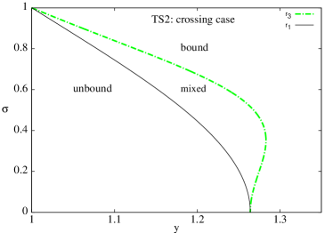
Following the same procedure of comparison of free energies, the phase diagram is obtained in the $y$-$\sigma$ plane, as shown in Fig. 8. With the given initial conditions this model exhibits the mixed phase. One sees two transitions: At low temperature we have a three-chain bound state that goes into the mixed state (green dash-dotted line in Fig. 8) and the mixed state melts into free chains (black solid line in Fig. 8). This latter transition coincides with the two-chain melting curve.

V.3 Model TS3: With crossing

Here three chains have repulsive interaction as in TS2, but we consider a different generalization that favours three-chain bubbles.

• Walks can cross each other.

• $y_{12}=y_{23}=y_{31}=y,~{}y_{123}=\frac{1}{y}$.

• $\sigma_{12}=\sigma_{23}=\sigma_{31}=\sigma,~{}\sigma_{123}=\frac{1}{\sigma}$.

Here $\sigma<1$ and therefore $\sigma_{123}>1$. Two-chain bubbles are penalized by $\sigma$ but $\sigma_{123}$ favours three-chain bubbles.

Figure 9: Model TS3: the three-chain phase diagram in the $y$-$\sigma$ plane. The unbound, the bound, and the Efimov states are shown. The dark (black) line representing the two-chain melting curve, is not present in the three-chain case. There is no mixed phase.

However the recursion relations are same as for TS2 given by Eqs. (13a)-(13i). The initial conditions are

$$a_{0}=1,b_{0}=1,c_{0}=y,d_{0}=y^{2},e_{0}=y^{2},$$

$$f_{0}=y^{4},g_{0}=y\sigma,h_{0}=y^{2}\sigma,i_{0}=y^{3}\sigma.$$ (15)

Following the same procedure of comparison of free energies, the Efimov state is obtained and is shown in Fig. 9.

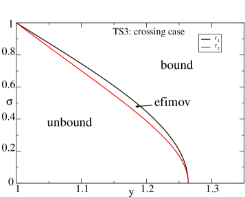
VI Energy diagram

The first order nature of the phase transitions can be determined from the behaviour of the average energy. For that we first validate, with a direct calculation of the free energy, the identifications of the phases done in the previous sections.

Figure 10: The fixed point values (circles) of grand canonical $z$ are compared with the canonical partition function $Q_{\rm tot}^{1/3N}$ (solid line). The values of the mixed phase partition function $(b_{n}d_{n})^{1/3N}$, are shown by the dash-dotted (green) line. Here $N=2^{26}$ is the length of each polymer.

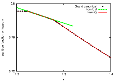
In the grand canonical approach, we determine its fixed point value of fugacity $z$ (See Sec. III), for given values of $y$ and $\sigma$. These are shown in Fig. 10. Based on the idea of the various phases, the total partition functions $Z_{\rm tot}$ and $Q_{\rm tot}$ for the two-chain and the three chain cases in the fixed length ensemble can be written as

$$Z_{\rm tot} = b_{n+1}^{2}+d_{n+1},$$ (16)

$$Q_{\rm tot} = f_{n+1}+b_{n+1}^{3}+2d_{n+1}b_{n+1},$$ (17)

in terms of the subpartition functions $b_{n+1}$, $d_{n+1}$, and $f_{n+1}$. A comparison of the grand canonical partition function $z$ and the canonical one $Q_{\rm tot}^{1/3N}$ for polymers of length $N=2^{n+1}$ with $n=25$, is shown in Fig. 10. The figure also shows the partition function for the mixed phase $[b_{n}d_{n}]^{1/3N}$ vs $y$. Armed with this agreement, the average energy calculation can be simplified. The total average energies of the two-chain system ($E_{\rm tot}$) and the three-chain system (${\cal E}_{\rm tot}$) can be written as

$$E_{\rm tot} = \frac{d_{n}E_{d_{n}}}{Z_{tot}},$$ (18)

$${\cal E}_{\rm tot} = \frac{f_{n}E_{f_{n}}+2b_{n}d_{n}E_{d_{n}}}{Q_{\rm tot}}$$ (19)

where $E_{d_{n}}$ and $E_{f_{n}}$ are the energies corresponding to the partition functions $f_{n}$ and $d_{n}$, all of which can be computed iteratively. The recursion relations for the energies for model TS1 are given in Appendix B.

The three-chain average energy per bond, $\langle E\rangle={\cal E}_{\rm tot}/N$, is shown for model TS1 in Fig. 11. Fig. 11(a) is for $\sigma=1.25$. The three-chain average energy (marked as 1) is compared to the two-chain average energy (marked as 2). This shows the nonzero three-chain average energy, even though the duplex average energy is zero.

Figure 11: Plot of the average energy per bond with $y$, for Model TS1. Here $\epsilon=1$. The vertical lines are to show the discontinuity in the energy curves. The three-chain average energy (marked as 1) is compared to the two-chain average energy (marked as 2). (a) For $\sigma=1.25$. (b) For $\sigma=0.5$. The first order transition for the two chain model is consistent with experimental findings.

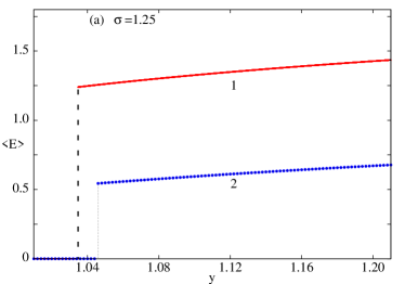
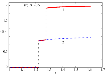
Fig. 11(b) is for $\sigma=0.5$. The three-chain average energy (marked as 1) is compared to the two-chain average energy (marked as 2). The transition from the unbound to the mixed state is at the same temperature as the two-chain case, i. e., at $y_{c}(\sigma)$. The transition from the mixed state to the bound state occurs for $y>y_{c}(\sigma)$ (lower temperature).

The average energy curve in Fig. 11(a) marked as 1 shows only one jump, where as in Fig. 11(b) the average energy curve marked as 1 shows two jumps. In the latter case the two transitions are from the unbound to the mixed state and from the mixed to the three-chain bound state.

VII Discussion

All the models and results are given below for easy reference. A large class of models can be defined distinguished by the nature of interactions and the cooperativity factors. Many of the models are not discussed in details in this paper but the results are stated in Table. 1.

We discuss briefly model TSnull, because it is a reference model that allows us to understand the origin of the three-body effects, either Efimov or the mixed state, in the other models. In model TSnull, instead, the duplex and the triplex melting curves superpose exactly and no special three-body effect is present. That is due to chains $1$ and $3$ being uncoupled, so that the three-chain behaviour is dictated by the independent behaviour of the chain pairs $12$ and $13$.

Any model feature that effectively couples chains $1$ and $3$ causes the presence of cooperative three-body effects. The coupling can be induced by conditions on the contact energies $y(>1)$’s, on the weights $\sigma$’s for bubble opening and closure, or by the presence of the noncrossing constraint. Depending on the combination of those conditions, a few models, like TS2, show the mixed state while the others, like TS3, show the Efimov-like state. But for model TS1 we get both of the states though in different regimes of $\sigma$ and $y$.

If we compare models TS2 and TS3, in both of them the overall energy of the triplex state is the same as for the duplex state due to the repulsive nature of the three-chain interaction ($y_{123}>1$), but there is a bias in TS2 penalizing the bubble opening or closure in the triplex state. This biasing seems to favor the mixed state in TS2, by entropically destabilizing the triplex state. On the other hand, the conditions on the $\sigma$’s used in TS3 remove this bias and leave an effective coupling between chains $1$ and $3$ that seems to favour the Efimov state by entropically stabilizing the triplex state. Intriguingly, the Efimov state is stabilized through the same mechanism in model TS4 as well, even in the absence of the energetic coupling between chains $1$ and $3$ that is present in both models TS2 and TS3.

The presence of the noncrossing constraint further complicates things. Its effect on a two-chain system is equivalent to a rescaling of $\sigma$ by a $1/\sqrt{2}$ factor in the presence of crossing, thus causing the entropic destabilization of the duplex state. In a three-chain system a different rescaling by a $1/\sqrt{3}$ factor would be needed to obtain Eq. (9f) from the corresponding Eq. (13f) in the presence of crossing. As a consequence, the simultaneous presence of two-chain and three-chain bubbles does not allow to establish any simple mapping between the noncrossing model and a $\sigma$-rescaled crossing model. Yet, one can argue on this basis that the noncrossing constraint induces an entropic destabilization stronger for the triplex state than for the duplex. In fact, in model TS5 the coupling between chains $1$ and $3$ is due only to the noncrossing constraint, and the mixed phase emerges, consistent with the above observation.

Finally, in model TS1 a further coupling is caused by the choice of the $\sigma$’s weights that either penalizes (for $\sigma<1$) or favours (for $\sigma>1$) the bubble opening or closure in the triplex state. As a result, the mixed and the Efimov states coexist in the same phase diagram, with the Efimov state being present in the $\sigma>1.14458$ part of the phase diagram.

For $\sigma=0$ all the models are like the Y-fork model and come out to be the same, and $y_{c}(0)=1.2640847353...$ denotes the melting for both the two- and the three-chain systems.

All the models that we considered show first order phase transitions, with discontinuities in the average energy. This is an effect due to the fractal lattice since similar DNA models defined through directed polymers on the Euclidean lattice show second order melting transitions when $\sigma>0$ unzip2 . Only for the Y-fork model the melting transition is first-order on the Euclidean lattice as well.

VIII Conclusion

Working on regular fractal lattices has the advantage of allowing for exact solutions. Consequently, even very tiny and elusive effects, as those observed in this paper, can be highlighted without the doubts that can affect numerical simulations on Euclidean lattices. For these reasons, we believe our results are very intriguing and deserve attention by experimentalists.

In particular we have shown that, when an extra weight $\sigma$ for the two- and the three-chain bubble opening and closure is introduced the Efimov-DNA, a loosely bound three-chain state where no two are bound, occurs even in $d<2$. What is remarkable is the emergence of a new state, to be called a mixed state, where locally any two are bound keeping the third-strand always free but in a global view no one is completely free. The intermediate phase evolves as a separate phase whereas the Efimov state is a crossover.

The cooperativity factor $\sigma$ acts as a control parameter for the bubbles on DNA. We see that for both Efimov-DNA and the mixed phase, the existence of bubbles is a necessity. There is no such effect at $\sigma=0$, despite a duplex melting transition. Since there is no distance defined on the fractal lattices, the results of the paper do not necessarily require any induced long range interaction. Our results for a large varieties of models rather imply that a necessary mathematical condition for both the phenomena is the bubble induced thermodynamic phase transition.

Why DNA? The native interaction involving base pairs at the same monomer position on the two strands is very special to DNA. The effects we are modeling depend crucially on this feature, even though the strands can be taken as ordinary polymers. For ordinary polymers, monomers interact irrespective of their locations on the chain SMB2013 which vitiates the quantum - polymer mapping, and the models used here. Fractal surfaces are routinely generated in the laboratory but we are not aware of any attempt of adsorption of DNA or any other polymers on such fractal objects. The closest we are aware of is DNA adsorbed on a surface. E.g. a double stranded DNA on a lipid bilayer is known to behave like a two-dimensional self-avoiding random polymer maier1999 . We feel that such systems of DNA in low dimensions might show some signature of the “mixed phase”. We tend to believe that DNA adsorbed on a surface is the most natural choice for seeing the mixed phase predicted in this paper.

The existence of a bound state involving two otherwise denaturated strands of DNA due to the presence of a third strand (the Efimov state) or the opening of a double for the presence of a third strand, might have important implications for biological processes. Many biological processes involve three strands, especially strand exchange. Whether the emergent structures resemble the phases obtained in this paper remains a matter of speculation. We expect our results will stimulate further theoretical calculations in higher dimensions and new experiments to look for signatures of the proposed mechanisms.

Model	Parameters	Parameters	Results
TS1 (Noncrossing)	$y_{12}=y_{23}=y,y_{31}=1$	$\sigma_{ij}=\sigma$, $\sigma_{123}=1$	Efimov, Mixed
TS2 (Crossing)	$y_{ij}=y,y_{123}=1/y$	$\sigma_{ij}=\sigma,\sigma_{123}=1$	Mixed
TS3 (Crossing)	$y_{ij}=y,y_{123}=1/y$	$\sigma_{ij}=\sigma,\sigma_{123}=1/\sigma$	Efimov
TS4 (Crossing)	$y_{12}=y_{23}=y,y_{31}=1$	$\sigma_{ij}=\sigma$, $\sigma_{123}=1/\sigma$	Efimov
TS5 (Noncrossing)	$y_{12}=y_{23}=y,y_{31}=1$	$\sigma_{ij}=\sigma$, $\sigma_{123}=1/\sigma$	Mixed
TSnull (crossing)	$y_{12}=y_{23}=y,y_{31}=1$	$\sigma_{12}=\sigma_{23}=\sigma,\sigma_{31}=1,\sigma_{123}=1$	Nothing

Table 1: The results obtained for the three-chain models. The subscripts label the chains, $i,j=1,2,3$. The models are distinguished by the conditions satisfied by the parameters. The new phases obtained are also flashed in this table. Models TS4 and TSnull require a different set of recursion relations, that use 14 generating functions, as shown in Appendix C.

Appendix A Diagrams for recursion relation

In this appendix we show how to generate the recursion relations for $d_{n}$ for the noncrossing case as an example. The sub-partition function for $n+1$ can be expressed in terms of the various partition functions of the $n$th generation as shown in Fig. 12. For the crossing case, one would need a factor of 2 for two possibilities of the bubble in Fig. 3.

Figure 12: Diagrams showing Eq. (8). A combinatorial factor 2 is needed for the second diagram on the right hand side for Eq. (2d), as explained in Fig. 3.

Appendix B Recursion relations for energies

For model TS1, one may associate an energy for each of the sub-partition functions. These energies obey the following recursion relations:

$$E_{c_{n+1}} = 2E_{c_{n}}$$ (20)

$$E_{d_{n+1}} = \frac{1}{d_{n+1}}\left[2d_{n}^{2}E_{d_{n}}+c_{n}^{2}d_{n}E_{d_{n}}+2c_{n}^{2}d_{n}E_{c_{n}}+2g_{n}^{2}b_{n}E_{g_{n}}\right]$$ (21)

$$E_{e_{n+1}} = 2E_{e_{n}}$$ (22)

$$E_{f_{n+1}} = \frac{1}{f_{n+1}}\left[2f_{n}^{2}E_{f_{n}}+e_{n}^{2}f_{n}E_{f_{n}}+2e_{n}^{2}f_{n}E_{e_{n}}+h_{n}^{2}d_{n}E_{d_{n}}+2d_{n}h_{n}^{2}E_{h_{n}}+2b_{n}i_{n}^{2}E_{i_{n}}\right]$$ (23)

$$E_{g_{n+1}} = \frac{1}{g_{n+1}}\left[(b_{n}+c_{n})a_{n}g_{n}E_{g_{n}}+g_{n}a_{n}c_{n}E_{c_{n}}\right]$$ (24)

$$E_{h_{n+1}} = \frac{1}{h_{n+1}}\left[h_{n}E_{h_{n}}(a_{n}e_{n}+b_{n}c_{n})+h_{n}(a_{n}e_{n}E_{e_{n}}+b_{n}c_{n}E_{c_{n}}\right]$$ (25)

$$E_{i_{n+1}} = \frac{1}{i_{n+1}}\left[i_{n}E_{i_{n}}(c_{n}e_{n}+d_{n}a_{n})+i_{n}(c_{n}e_{n}E_{c_{n}}+c_{n}e_{n}E_{e_{n}}+d_{n}a_{n}E_{d_{n}})+g_{n}^{2}h_{n}E_{h_{n}}+2g_{n}^{2}h_{n}E_{g_{n}}\right]$$ (26)

These are used to calculate the energies in Sec. VI.

Appendix C Recursion relations for TS4 and TSnull models

In this appendix we show the recursion relations used for TS4 and TSnull models. In both cases we need to use an expanded set of 14 generating functions, because the conditions on the $y$’s and $\sigma$’s parameters cause the chain pair $13$ to have different properties with respect to the two other pairs $12$ and $23$. Therefore, the two chain generating functions $c_{n}$, $d_{n}$, $g_{n}$ and the two three-chain bubble opening/closure generating functions $h_{n}$, $i_{n}$ needs to be considered twice. Note that if the noncrossing constraint is present, conditions such as $y_{12}=y_{23}=y,y_{31}=1$ are equivalent to $y_{ij}=y,y_{123}=1/y$ and there is no need for an extended set of generating functions.

$$a_{n+1} = a_{n}^{2},$$ (27)

$$b_{n+1} = b_{n}^{2}+a_{n}^{2}b_{n},$$ (28)

$$c_{12,n+1} = c_{12,n}^{2},$$ (29)

$$c_{13,n+1} = c_{13,n}^{2},$$ (30)

$$d_{12,n+1} = d_{12,n}^{2}+2g_{12,n}^{2}b_{n}+c_{12,n}^{2}d_{12,n},$$ (31)

$$d_{13,n+1} = d_{13,n}^{2}+2g_{13,n}^{2}b_{n}+c_{13,n}^{2}d_{13,n},$$ (32)

$$e_{n+1} = e_{n}^{2}$$ (33)

$$f_{n+1} = f_{n}^{2}+e_{n}^{2}f_{n}+2h_{12,n}^{2}d_{12,n}+h_{13,n}^{2}d_{13,n}+2i_{12,n}^{2}b_{n}+i_{13,n}^{2}b_{n},$$ (34)

$$g_{12,n+1} = a_{n}g_{12,n}(b_{n}+c_{12,n}),$$ (35)

$$g_{13,n+1} = a_{n}g_{13,n}(b_{n}+c_{13,n}),$$ (36)

$$h_{12,n+1} = h_{12,n}(a_{n}e_{n}+b_{n}c_{12,n}),$$ (37)

$$h_{13,n+1} = h_{13,n}(a_{n}e_{n}+b_{n}c_{13,n}),$$ (38)

$$i_{12,n+1} = i_{12,n}(c_{12,n}e_{n}+d_{12,n}a_{n})+g_{12,n}^{2}h_{12,n}+g_{12,n}g_{13,n}h_{13,n},$$ (39)

$$i_{13,n+1} = i_{13,n}(c_{13,n}e_{n}+d_{13,n}a_{n})+2g_{12,n}g_{13,n}h_{12,n}.$$ (40)

References

- (1) J. Maji, S. M. Bhattacharjee, F. Seno, and A. Trovato, New J. Phys. 12 (2010) 083057.
- (2) J. Maji and S. M. Bhattacharjee, Phys. Rev. E 86, 041147 (2012).
- (3) T. Pal, P. Sadhukhan, and S. M. Bhattacharjee, Phys. Rev. Lett. 110, 028105 (2012).
- (4) The complete breaking of the base pairing hydrogen bonds of a dsDNA is called the melting of DNA. It is also known as the unbinding transition, or the denaturation transition. These names will be used interchangeably. The two free strands in the “molten” state are also called denatured DNA. The force induced opening is called unzipping of DNA unzip1 ; unzip2 ; unzip3 ; kapri .
- (5) S. M. Bhattacharjee, J. Phys. A 33, L423 (2000).
- (6) D. Marenduzzo, A. Trovato and A. Maritan, Phys. Rev. E 64, 031901 (2001).
- (7) D. Marenduzzo, S. M. Bhattacharjee, A. Maritan, E. Orlandini, and F. Seno, Phys. Rev. Lett. 88, 028102 (2001).
- (8) R. Kapri, S. M. Bhattacharjee, and F. Seno, Phys. Rev. Lett. 93, 248102 (2004)
- (9) V. Efimov, Phys. Lett. B 33,563 (1970).
- (10) V. Efimov, Sov. J. Nucl. Phys. 12, 589, 1971.
- (11) L. Thomas, Phys. Rev. 47, 903 (1935).
- (12) G. Felsenfeld, D. R. Davies, and A. Rich, J. Am. Chem. Soc. 79, 2023 (1957).
- (13) F. A. Buske, J. S. Mattick, and T. L. Bailey, RNA Biology 8, 427(2011).
- (14) M. D. Frank-Kamenetskii, S. M. Mirkin, Annu Rev Biochem. 64, 65 (1995).
- (15) I. Radhakrishnan and D. J. patel, Biochem. 33, 11405 (1994).
- (16) E. N. Nikolova , F. L. Gottardo, and H. M. Al-Hashimi, J. Am. Chem. Soc. 134 3667 (2012).
- (17) R.W. Roberts and D.M. Crothers, Science 258, 1463 (1992)
- (18) P. E. Nielsen, Annu. Rev. Biophys. Biomol. Struct. 24, 167 (1995); Sci. Am. 99, 64 (2008).
- (19) A. Ray and B. Nordén, FASEB J. 14, 1041 (2000).
- (20) J. Sun, T. Garestier, and C. Hélène, Curr. Op. in Str. Bio. 6, 327 (1996).
- (21) L. Betts, J.A. Losey, J.M. Veal, and S.R. Jordan, Science 270 5243 (1995)
- (22) D. P. Arya, R.L. Coffee, and L. Xue, Bioorg. Med. Chem. Lett. 14 4643 (2004).
- (23) M. Duca, P. Vekhopp, K. Oussedik, L. Halby, and P. B. Arimondo, Nucl. Acids Res. 36, 5123 (2008).
- (24) A. Jain, G. Wang, and K. M. Vasquez, Biochimie 90 1117 (2008).
- (25) N. T. Thoung and C. Hélène, Angew. Chem. Int. Ed. 32, 666 (1993).
- (26) This is similar to the quantum mechanics result of at least one bound state in any attractive short range potential for , while in higher dimensions the potential has to attain a critical strength to form a bound state.
- (27) D. Dhar, J. Math. Phys. 19, 1 (1978).
- (28) M. Di Stasio, F. Seno, and A. L. Stella, J. Phys. A: Math. Gen. 25, 3891 (1992).
- (29) S. Kumar and Y. Singh, J. Stat. Phys. 89, 981 (1997).
- (30) Y. Gefen, B.B. Mandelbrot, and A. Aharony, Phys. Rev. Lett. 45, 855 (1980).
- (31) M. Knezevic and J. Vannimenus, Phys. Rev. Lett. 56, 1591 (1986).
- (32) S. Elezovic-Hadzic and I. Zivic, J. Stat. Mech. Theo. and Exp., Article Number: P02045 (2013)
- (33) S. C. Chang, L. C. Chen, and H. Y. Lee, Physica A, 392, 1776 (2013)
- (34) D. Dhar and J. Vannimenus, Jour de Physique 19 (1986).
- (35) D. Poland and H.A. Scheraga, J. Chem. Phys. 85, 1456 (1966)
- (36) D. Dhar and Y. Singh, in Statistics of Linear Polymers in Disordered Media, edited by B. K. Chakraborty (Elsevier, Amsterdam, 2005)
- (37) E. Orlandini, F. Seno, A. L. Stella, and M. C. Tesi, Phys. Rev. Lett. 68, 488 (1992).
- (38) S.A. Kozyavkin, S.M. Mirkin, and B.R. Amirikian, J Biomol. Struct. Dyn. 5, 119 (1987).
- (39) See, for instance, discussion in Y. Kafri, D. Mukamel, L. Peliti, Phys. Rev. Lett. 85, 4988 (2000).
- (40) See, e.g., S.M. Bhattacharjee, A. Giacometti, and A. Maritan, J. Phys.: Condens. Matter 25, 503101 (2013).
- (41) B. Maier and J. Rädler, Phys. Rev. Lett. 82, 1911 (1999).