The spin-polarized $\nu=0$ state of graphene: a spin superconductor

Abstract

We study the spin-polarized $\nu=0$ Landau-level state of graphene. Due to the electron-hole attractive interaction, electrons and holes can bound into pairs. These pairs can then condense into a spin-triplet superfluid ground state: a spin superconductor state. In this state, a gap opens up in the edge bands as well as in the bulk bands, thus it is a charge insulator, but it can carry the spin current without dissipation. These results can well explain the insulating behavior of the spin-polarized $\nu=0$ state in the recent experiments.

I Introduction

In a magnetic field, monolayer and bilayer graphenes display unconventional Landau-level (LL) spectrum, where the zeroth LL locates the charge neutrality point and has equal electron and hole compositions.ref1 ; ref2 ; ref3 The zeroth LL is fourfold degenerate in monolayer graphene owing to the spin and valley degeneracies, and it is eightfold degenerate in bilayer one due to the additional orbit (or layer) degeneracy. While under a high magnetic field, electron-electron (e-e) interaction can lift the LL degeneracy,ref2 ; ref3 ; ref6 ; ref7 ; ref8 ; ref9 ; ref10 ; ref11 ; ref12 ; ref13 ; ref14 ; ref15 leading to broken symmetry quantum Hall states and manifesting further integer Hall plateaus outside the normal sequence, which have been experimentally observed.ref16 ; ref17 ; ref18 ; ref19 ; ref20 ; ref21 ; ref22 ; ref23 ; ref24 ; ref25 ; ref26 ; ref27 ; ref28 ; ref29 ; ref30

Recently, the splitting of the zeroth LL has attracted considerable theoretical and experimental interest.ref6 ; ref7 ; ref8 ; ref9 ; ref10 ; ref11 ; ref12 ; ref13 ; ref14 ; ref15 ; ref16 ; ref17 ; ref18 ; ref19 ; ref20 ; ref21 ; ref22 ; ref23 ; ref24 ; ref25 ; ref26 ; ref27 ; ref28 ; ref29 ; ref30 ; ref31 ; ref32 ; ref33 ; ref34 ; ref35 ; ref36 A bulk gap opening around the energy $E=0$ is found and a zero Hall conductance plateau at the filling factor $\nu=0$ has been observed. Both the spin-polarized and valley-polarized $\nu=0$ states are suggested. At $\nu=0$, although the Hall conductance shows a plateau, the longitudinal resistance experimentally exhibits an insulating behavior,ref16 ; ref17 ; ref18 ; ref19 ; ref20 ; ref21 ; ref22 ; ref23 ; ref24 ; ref25 ; ref26 ; ref27 ; ref28 ; ref29 ; ref30 which is very different with the zero longitudinal resistance in the conventional quantum Hall effect.

In the valley-polarized $\nu=0$ state, the valley splitting is larger than the spin splitting and it is a spin singlet state. Now not only $\nu=0$, but also the spin-up and spin-down filling factors $\nu_{\uparrow}=\nu_{\downarrow}=0$.ref36 In this case, the system is without an edge state as shown in Fig.1(a), so it is insulating for both bulk and edge states, which is consistent with the experiment results.

On the other hand, when the spin splitting is larger than the valley splitting, the system is in the spin-polarized $\nu=0$ state.ref7 ; ref31 Now, however, $\nu_{\uparrow}$ and $\nu_{\downarrow}$ are not equal to zero although $\nu=\nu_{\uparrow}+\nu_{\downarrow}=0$. A $+$ valley spin-up ($+\uparrow$) LL is occupied by electron and a $-$ valley spin-down ($-\downarrow$) LL is occupied by hole, leading to a pair of counter-propagating edge states [see Fig.1(b)] that can carry both spin and charge currents.ref31 ; ref32 ; ref33 ; ref34 ; ref35 ; ref36 Some theoretical works have predicted the spin Hall effect in this case.ref34 ; ref35 Particularly, due to the presence of the edge states, the longitudinal resistance is $(|\nu_{\uparrow}|+|\nu_{\downarrow}|)e^{2}/h$ and the system should not show an insulating behavior, although a bulk gap exists. However, experiment works have clearly exhibited an insulating behavior and the longitudinal resistance increases quickly with decreasing temperature regardless whether it is a monolayer or bilayer graphene.ref17 ; ref20 ; ref21 ; ref27 ; ref28 ; ref30 This is very different from the theoretical prediction and seems to indicate the disappearance of the edge states. Some studies mention that the possible reason for this discrepancy is that the counter-propagating edge states are destroyed by disorders.ref27 ; ref32 ; ref33 ; ref35 ; ref36 But the sizes of the experimental samples are only a few micrometers, too short to destroy the edge states by localizing the edge electrons. Furthermore, the disorder effect can not explain strong increase of the longitudinal resistance at low temperature. In short, this discrepancy is still lack of a reasonable explanation.

In this paper, the spin-polarized $\nu=0$ state in graphene under a strong magnetic field is investigated. By considering the unavoidable electron-hole (e-h) attractive interaction, we find that electrons at $+\uparrow$ LL and holes at $-\downarrow$ LL can form spin-triplet e-h pairs. This e-h pair gas can condense at low temperature, leading to the transition to a spin superconductor phase (spin-triplet exciton condensation state)ref37 associated with the opening of an energy gap for the edge states. Thus, the system exhibits an insulating behavior, consistent with experimental observations.ref17 ; ref20 ; ref21 ; ref27 ; ref28 ; ref30

The remainder of this paper is organized as follows. In Sec. II, we introduce the Hamiltonian in the tight-binding representation and derive the formula of the spin-superconductor order parameter. The results are discussed in Sec. III. Finally, the conclusion is presented in Sec. IV.

II Model and formulation

Let us consider a graphene nanoribbon in a magnetic field. In the tight-binding representation, its Hamiltonian is $\mathcal{H}=\mathcal{H}_{0}+\mathcal{H}_{I}$, where

$$\mathcal{H}_{0} = \sum\limits_{{\bf i},\sigma}(\epsilon_{\bf i}-\sigma M)a^{\dagger}_{{\bf i}\sigma}a_{{\bf i}\sigma}+\sum\limits_{{\bf i},{\bf i}^{\prime},\sigma}t_{{\bf i}{\bf i}^{\prime}}e^{i\phi_{{\bf i}{\bf i}^{\prime}}}a^{\dagger}_{{\bf i}\sigma}a_{{\bf i}^{\prime}\sigma}+H.c.$$

$$\mathcal{H}_{I} = \sum\limits_{{\bf i},{\bf i}^{\prime},\sigma,\sigma^{\prime}({\bf i}\sigma\not={\bf i}^{\prime}\sigma^{\prime})}U_{{\bf i}{\bf i}^{\prime}}a^{\dagger}_{{\bf i}\sigma}a_{{\bf i}\sigma}a^{\dagger}_{{\bf i}^{\prime}\sigma^{\prime}}a_{{\bf i}^{\prime}\sigma^{\prime}},$$ (1)

represent the free part and the e-e Coulomb interaction part of the Hamiltonians, respectively. Here $a^{\dagger}_{{\bf i}\sigma}$ ($a_{{\bf i}\sigma}$) is the electron creation (annihilation) operator at sites ${\bf i}$ with spin $\sigma$. $\epsilon_{\bf i}$ is the on-site energy, and $M$ is spin splitting energy which origins from both the Zeeman effect and the spin polarization induced by the e-e interaction. The second term in $\mathcal{H}_{0}$ represents the hopping between the site ${\bf i}$ and ${\bf i}^{\prime}$. Because of the presence of a magnetic field $B$, a phase $\phi_{{\bf i}{\bf i}^{\prime}}=\int_{{\bf i}}^{{\bf i}^{\prime}}{\bf A}\bullet d{\bf l}/\phi_{0}$ ($\phi_{0}=\hbar/e$) is attached in the hopping element $t_{{\bf i}{\bf i}^{\prime}}$.ref38 $\mathcal{H}_{I}$ is the e-e interaction and $U_{{\bf i}{\bf i}^{\prime}}$ is the interaction strength. This Hamiltonian $\mathcal{H}$ can describe both monolayer and bilayer graphene ribbons with arbitrary edge chirality. Considering the ribbon periodicity, the site indices ${\bf i}$ can be represented as ${\bf i}=(n,j)$ with the slice cell indices $n$ and the atomic indices $j$ in a cell ($j=1,2,\ldots,N$ and $N$ is the total atom number in a cell). Then the Hamiltonian can be rewritten as:

$$\mathcal{H}_{0} = \sum\limits_{n,\sigma}\vec{a}^{\dagger}_{n\sigma}({\bf H}_{0}-\sigma M)\vec{a}_{n\sigma}+\sum\limits_{n,\sigma}\vec{a}^{\dagger}_{n\sigma}{\bf H}_{1}\vec{a}_{n-1\sigma}+H.c.$$

$$\mathcal{H}_{I} = \sum\limits_{n,n^{\prime},\sigma,\sigma^{\prime}}\vec{n}^{\dagger}_{n\sigma}{\bf U}_{n-n^{\prime}}\vec{n}_{n^{\prime}\sigma^{\prime}},$$ (2)

where $\vec{a}_{n\sigma}=(a_{n1},a_{n2},\ldots,a_{nN})^{T}$ and $\vec{n}_{n\sigma}=(a^{\dagger}_{n1}a_{n1},a^{\dagger}_{n2}a_{n2},\ldots,a^{\dagger}_{nN}a_{nN})^{T}$. ${\bf H}_{0}$, ${\bf H}_{1}$, and ${\bf U}_{n-n^{\prime}}$ are the intra-cell Hamiltonian, hopping term between two nearest-neighbor cells, and the e-e interaction. By taking the Fourier transformation $\vec{a}_{n\sigma}=\frac{1}{\sqrt{L}}\sum_{k}e^{inak}\vec{a}_{k\sigma}$ with the nanoribbon length $La$ and the cell length $a$, the Hamiltonian $\mathcal{H}$ can be written as: $\mathcal{H}_{0}=\sum_{k,\sigma}\vec{a}^{\dagger}_{k\sigma}({\bf H}_{k}-\sigma M)\vec{a}_{k\sigma}$ with ${\bf H}_{k}={\bf H}_{0}+{\bf H}^{\dagger}_{1}e^{iak}+{\bf H}_{1}e^{-iak}$, and

$$\mathcal{H}_{I}=\sum\limits_{\sigma,\sigma^{\prime},k,k^{\prime},q}\vec{a}^{\dagger}_{k-q\sigma}\vec{a}_{k\sigma}{\bf U}_{k-k^{\prime}}\vec{a}^{\dagger}_{k^{\prime}+q\sigma^{\prime}}\vec{a}_{k^{\prime}\sigma}$$ (3)

with ${\bf U}_{k}=\frac{1}{L}\sum_{n}e^{inak}{\bf U}_{n}$. In fact, ${\bf H}_{k}$ is the momentum-space Hamiltonian of the free system. Assuming that the eigen-wavefunctions and eigenvalues of ${\bf H}_{k}$ are $\vec{\Psi}^{(j)}_{k}$ and $\epsilon^{(j)}_{k}$: ${\bf H}_{k}\vec{\Psi}^{(j)}_{k}=\epsilon^{(j)}_{k}\vec{\Psi}^{(j)}_{k}$, we have ${\bf\mathcal{U}}_{k}^{\dagger}{\bf H}_{k}{\bf\mathcal{U}}_{k}={\bf\epsilon}_{k}$ with ${\bf\mathcal{U}}_{k}=(\vec{\Psi}^{(1)}_{k},\vec{\Psi}^{(2)}_{k},\ldots,\vec{\Psi}^{(N)}_{k})$ and ${\bf\epsilon}_{k}=diag(\epsilon^{(1)}_{k},\epsilon^{(2)}_{k},\ldots,\epsilon^{(N)}_{k})$. By taking a unitary transformation: $\vec{a}_{k\sigma}={\bf\mathcal{U}}_{k}\vec{b}_{k\sigma}$, $\mathcal{H}_{0}$ changes into $\mathcal{H}_{0}=\sum_{k\sigma}\vec{b}^{\dagger}_{k\sigma}({\bf\epsilon}_{k}-\sigma M)\vec{b}_{k\sigma}$.

Let us assume that the eigenvalues $\epsilon^{(j)}_{k}$ have been arranged according of their values from small to large and Fermi level $E_{F}$ is set at zero. The two nearest bands to $E_{F}$ are the spin-up $1+N/2$-th band and spin-down $N/2$-th band. Due to the presence of a magnetic field and the spin splitting energy $M$, the system consists of LLs and is spin-polarized. The spin-up $1+N/2$-th (spin-down $N/2$-th) band is denoted as $+\uparrow$ ($-\downarrow$) LL with its energy $\epsilon^{(1+N/2)}_{k}-M$ below ($\epsilon^{(N/2)}_{k}+M$ above) $E_{F}$, its carrier being electron-like (hole-like), and its band bending upward (downward) as shown in Fig.1(b). Now the system is at the spin-polarized $\nu=0$ state, in which a bulk gap $2M$ appears but two edge states cross at $E_{F}$. In the following, we focus on these two low-energy bands, and show that the e-e interaction $\mathcal{H}_{I}$ will create an energy gap for the edge states. Let us introduce the electron and hole annihilation operators: $b_{k\uparrow e}=b_{k\uparrow,1+N/2}$ and $b_{k\uparrow h}=b^{\dagger}_{k\downarrow,N/2}$. Then the free Hamiltonian $\mathcal{H}_{0}$ reduces to:

$$\mathcal{H}_{0}=\sum\limits_{k}[b^{\dagger}_{k\uparrow e}(\epsilon_{ke}-M)b_{k\uparrow e}+b^{\dagger}_{k\uparrow h}(\epsilon_{kh}-M)b_{k\uparrow h}]$$

with $\epsilon_{ke}=\epsilon^{(1+N/2)}_{k}$ and $\epsilon_{kh}=-\epsilon^{(N/2)}_{k}$.

As for $\mathcal{H}_{I}$, we take the following steps: 1) only the terms whose momenta satisfy $k=k^{\prime}+q$ in Eq.(3) are kept since the zero momentum e-h pairs are energetically more favorable; 2) we take the aforementioned unitary transformation and the e-h transformation; 3) we focus on the two low-energy bands; and 4) we assume that $U_{{\bf i}{\bf i}^{\prime}}=U_{c}$ while ${\bf i}={\bf i}^{\prime}$ and $U_{{\bf i}{\bf i}^{\prime}}=0$ otherwise, since the on-site e-e interaction is the dominant one. Then the interaction part $\mathcal{H}_{I}$ reduces to:

$$\mathcal{H}_{I}=-\sum\limits_{k,k^{\prime}}U_{kk^{\prime}}b^{\dagger}_{k^{\prime}\uparrow e}b^{\dagger}_{k^{\prime}\uparrow h}b_{k\uparrow h}b_{k\uparrow e},$$ (4)

where

$$U_{kk^{\prime}}=\frac{1}{L}\sum_{j}\mathcal{U}_{k^{\prime},jN/2}^{*}\mathcal{U}_{k,jN/2}U_{c}\mathcal{U}_{k,j1+N/2}^{*}\mathcal{U}_{k^{\prime},j1+N/2}$$

.

While at equilibrium, the spin-up electrons (holes) occupy the $+\uparrow$ ($-\downarrow$) LL and its edge state up to the energy $E=E_{F}=0$. This is a spin-polarized $\nu=0$ state and has $U(1)$ symmetry around $\sigma_{z}$-axis. Notice that the interaction $\mathcal{H}_{I}$ in Eq.(4) between an electron and a hole is attractive. This attractive interaction will not cause the e-h recombination, due to both the spin splitting and the hole band ($-\downarrow$ LL) is above the electron band ($+\uparrow$ LL).ref37 However, it can lead to a different instability of the spin-polarized $\nu=0$ state at low temperature, namely the electrons and holes can form e-h pairs which can then condense to a spin-triplet superfluid state.ref37 ; ref39 Notice here the spin splitting (or spin polarization) is a key factor for stable e-h pairs. Under the mean-field approximation, $\mathcal{H}_{I}$ changes into:

$$\mathcal{H}_{I}=\sum\limits_{k}\left[\Delta_{k}b^{\dagger}_{k\uparrow e}b^{\dagger}_{k\uparrow h}+\Delta_{k}^{*}b_{k\uparrow h}b_{k\uparrow e}\right],$$ (5)

where $\Delta_{k}\equiv-\sum_{k^{\prime}}U_{kk^{\prime}}\langle b_{k^{\prime}\uparrow h}b_{k^{\prime}\uparrow e}\rangle$ is the e-h pair condensation order parameter. So we have the total Hamiltonian $\mathcal{H}=\mathcal{H}_{0}+\mathcal{H}_{I}$:

$$\mathcal{H}=\sum\limits_{k}\left(\begin{array}[]{l}b^{\dagger}_{k\uparrow e},b_{k\uparrow h}\end{array}\right)\left(\begin{array}[]{ll}\epsilon_{ke}-M&\Delta_{k}\\ \Delta_{k}^{*}&M-\epsilon_{kh}\end{array}\right)\left(\begin{array}[]{l}b_{k\uparrow e}\\ b^{\dagger}_{k\uparrow h}\end{array}\right).$$ (6)

Now a gap $|\Delta_{k}|$ opens up in the edge bands [e.g. see Fig.1(c) and (d)], and it needs an energy $2|\Delta_{k}|$ to break up an e-h pair. So the e-h pair condensed state is stabler than the spin-polarized $\nu=0$ state and it is the ground state of the system at low temperature. Since the spins of the electrons and the holes are both up, the e-h pair is spin triplet but charge neutral. The condensed superfluid state is a spin superconductor while it is a charge insulator.ref37 ; ref40 It carrys spin current dissipationlessly, thus, its spin resistance is zero. The spin superconductor also posseses its own unique ’Meissner effect”.ref37 Now the system has two possible phases. One is the spin-polarized $\nu=0$ state (hereafter we named it as normal state for short) at high temperature. It has a bulk gap but two gapless edge bands crossover at the Fermi level, leading to the current flow through the edge states.ref31 ; ref32 ; ref33 ; ref34 ; ref35 ; ref36 In the normal phase, the system consists of $U(1)$ symmetry. The other is the spin superconductor state at low temperature, in which both bulk bands and edge bands consist of energy gaps at $E_{F}$. Notice that this phase is still a spin polarized one and its filling factor $\nu=0$ with $\nu_{\uparrow}=-\nu_{\downarrow}=1$. We name it as spin-superconductor spin-polarized $\nu=0$ state, or spin superconductor state for short. This phase does not contain $U(1)$ symmetry around any direction. In other words, the system breaks $U(1)$ symmetry with the phase transition from the normal phase to the spin superconductor phase.

III Results and discussions

From the definition of $\Delta_{k}$ and Hamiltonian (6), we obtain the the self-consistent equation of $\Delta_{k}$: $\Delta_{k}=-i\sum_{k^{\prime}}U_{k^{\prime}k}\int\frac{d\epsilon}{2\pi}f(\epsilon)(\frac{\Delta_{k^{\prime}}}{A}-\frac{\Delta_{k^{\prime}}}{A^{*}}),$ where $f(\epsilon)$ is Fermi distribution function and $A=(\epsilon-\epsilon_{k^{\prime}e}+M+i0^{+})(\epsilon+\epsilon_{k^{\prime}h}-M+i0^{+})-|\Delta_{k^{\prime}}|^{2}$. While at zero temperature, the above equation reduces to:

$$\Delta_{k}=\sum\limits_{k^{\prime}}U_{k^{\prime}k}\frac{\Delta_{k^{\prime}}}{\sqrt{(\epsilon_{k^{\prime}e}+\epsilon_{k^{\prime}h}-2M)^{2}+4|\Delta_{k^{\prime}}|^{2}}}.$$ (7)

From this equation, $\Delta_{k}$ can be self-consistently calculated. In the numerical calculations, we first consider the monolayer zigzag graphene ribbon with the ribbon transverse width $W=(3N/4-1)a_{0}$ and periodic cell length $a=\sqrt{3}a_{0}$. Here $a_{0}=0.142$nm is the distance between two nearest-neighbor carbon atoms. We only consider the nearest-neighbor hopping with its strength $t_{{\bf i}{\bf i}^{\prime}}=t=2.75$eV, which is set as the energy unit. The on-site e-e interaction $U_{c}=\frac{e^{2}}{4\pi\epsilon_{0}r}\approx\frac{3.69}{r/a_{0}}t$ with the distance $r$ between two electrons. $U_{c}\approx 14.75t$ if $r=a_{0}/4$.

Figure 1: (color online) (a) and (b) are the schematic diagrams of the energy spectrum structures for the valley-polarized and spin-polarized $\nu=0$ states, respectively. (c) and (d) show $\Delta_{k}$ (the blue dashed curves), and the energy spectra for the normal state (the black solid curves) and for the spin superconductor state (the red dotted curves). (c) is for the zigzag edge graphene ribbon with the parameters $N=200$, $U_{c}=15t$, $M=0.03t$, and $\phi=0.004$, and (d) is for the armchair edge graphene ribbon with the parameters $N=282$, $U_{c}=25t$, $M=0.05t$, and $\phi=0.007$.

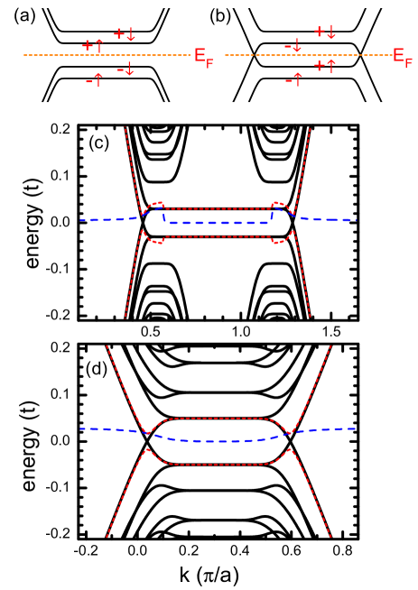
Fig.1(c) shows $\Delta_{k}$ and the energy spectrum. For the normal state, although it has a bulk gap due to the spin splitting energy $M$, two gapless edge states cross at the Fermi level and they can carry both charge and spin currents, causing the sample edge having a metallic behavior.ref31 ; ref32 ; ref33 ; ref34 ; ref35 ; ref36 On the other hand, for the spin superconductor state at low temperature, Fig.1(c) clearly exhibits a gap opening for the edge bands. Now both edge and bulk bands have the gaps, so it is a charge insulator, consistent with the experimental results.ref16 ; ref17 ; ref18 ; ref19 ; ref20 ; ref21 ; ref22 ; ref23 ; ref24 ; ref25 ; ref26 ; ref27 ; ref28 ; ref29 ; ref30 In this state, the spin current can dissipationlessly flow in it, because the condensed e-h pairs with spin $1$ can carry the spin super-current. Except for the edge states, other parts of the bands are almost the same for both normal and spin superconductor states and their LLs overlap, because that the carriers far away from Fermi level are not energetically favorable to form the e-h pairs. $\Delta_{k}$ is large for the edge bands but is vanishingly small for the bulk bands. This means that the condensed e-p pairs mainly distribute near the sample edge, and the spin super-current flows along the edges.

Up to now, we only consider the monolayer zigzag edge graphene. In fact, it is similar for graphene with other edge chirality as well as for a bilayer graphene. For example, Fig.1(d) shows $\Delta_{k}$ and the energy spectrum for the armchair edge graphene nanoribbon with the ribbon width $W=\frac{N-2}{4}\sqrt{3}a_{0}$ and cell length $a=3a_{0}$. The free Hamiltonian exhibits two gapless edge states. The e-h attractive interaction induces a gap in the edge states at the low temperature. The order parameter $\Delta_{k}$ is large for the edge bands but is very small for the bulk bands.

Figure 2: (color online) (a) and (b) show the energy spectra of the spin superconductor and the order parameter $\Delta_{k}$, respectively. The parameters are the same as in Fig.1(c).

Next, we study the zigzag edge graphene nanoribbon in detail. Fig.2(a) and 2(b) show the energy spectrum of spin superconductor state and $\Delta_{k}$ for different magnetic fields $\phi$ (here $2\phi=(3\sqrt{3}/2)a_{0}^{2}B/\phi_{0}$ is the magnetic flux in the honeycomb lattice). For all $\phi$, $\Delta_{k}$ exhibits peaks when the original bands cross at $E_{F}$ and $\Delta_{k}$ is small otherwise. With increasing $\phi$, $\Delta_{k}$ increases because a larger magnetic field leads to a smaller cyclotron radius of carriers, thus a stronger e-h attractive interaction $U_{k^{\prime}k}$. Particularly, for a large $\phi$, the edge-band gap can exceed the bulk-band gap (i.e. $2M$). In this case, the edge states disappear in the whole spin-polarized $\nu=0$ regime, as has been observed in the experiments.ref17 ; ref20 ; ref21 ; ref27 ; ref28 ; ref30

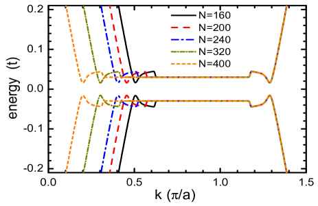
Fig.3 shows the energy spectrum of spin superconductor state for different width of nanoribbon. The results exhibit that both the edge-band gap and bulk-gap gap are almost independent with the width $N$. Because while under the high magnetic field the edge states and LLs in the spin-polarized state are independent with the width of nanoribbons.

Figure 3: (color online) The energy spectra for the spin superconductor state for the different width of nanoribbon. The parameters are the same as in Fig.1(c).

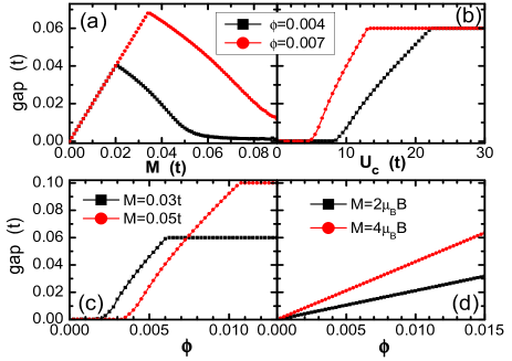
Let us study the effect of the system parameters on the energy gap. Here the gap is defined as the one of whole energy spectrum, equal to the smaller one of the bulk and the edge gaps. The gap is independent of the width $N$ of nanoribbon. Fig.4(a), (b), and (c) show the gap versus the spin splitting energy $M$, the e-e interaction strength $U_{c}$, and the magnetic flux $\phi$, respectively. With increase of $M$, the gap first increases due to the rising of the bulk gap, and then decreases. As for the gap versus $U_{c}$, there exists a threshold $U_{c}^{t}$ [see Fig.4(b)]. While $U_{c}<U_{c}^{t}$, the gap is almost zero, but while $U_{c}>U_{c}^{t}$, the gap increases quickly. When the gap reaches the bulk gap $2M$, it hardly increases further. In this case, although the edge gap can further increase, the gap of whole energy spectrum is decided by the bulk gap. The results of the gap vs. $\phi$ is similar to the one of the gap vs. $U_{c}$ since the increase of $\phi$ strengthens the effective e-h interaction $U_{kk^{\prime}}$. In an experiment, normally the spin splitting energy $M$ linearly rises with a magnetic field $B$. So in Fig.4(d), we show the gap vs. $\phi$ while $M=2\mu_{B}B$ and $4\mu_{B}B$. The results clearly exhibit that the gap linearly rises and the edge gap is always larger than the bulk gap. Now the edge states disappear in all $\phi$ value, which is well consistent with the experiment results.ref16 ; ref17 ; ref18 ; ref19 ; ref20 ; ref21 ; ref22 ; ref23 ; ref24 ; ref25 ; ref26 ; ref27 ; ref28 ; ref29 ; ref30 While $\phi=0.001$, $B$ is about 25 Tesla, and the gaps are about 3meV and 6meV for $M=2\mu_{B}B$ and $4\mu_{B}B$ respectively, to give rise to the corresponding critical temperatures of the phase transition to be about 30K and 60K.

Figure 4: (color online) The gap versus $M$ (a), $U_{c}$ (b), and $\phi$ (c and d). The unmentioned parameters are the same as Fig.1(c).

Finally, we notice that a recent experiment has simultaneously measured the resistance and the nonlocal resistance in graphene under a magnetic field.ref21 They find that the device is insulator at neutrality point with $\nu=0$. But, they also see that the nonlocal resistance increases rapidly at low temperature, and shows clearly that a spin current is flowing through the device. These findings can well be explained by the presence of a spin superconducting $\nu=0$ state.

IV conclusions

In summary, the spin-polarized $\nu=0$ state of the graphene under a magnetic field is investigated. We find that it has two phases, one is the normal phase at high temperature and other is the spin superconductor phase at low temperature. The $U(1)$ symmetry is destroyed under the phase transition from the normal phase to a spin superconductor. For the spin superconductor phase, both edge and bulk bands contain gaps, so it is a charge insulator, but the spin current can flow without dissipation. With the picture of the spin superconductor, many results from recent experiments can be well understood.

References

- (1) A.H. Castro Neto, F. Guinea, N.M.R. Peres, K.S. Novoselov, and A.K. Geim, Rev. Mod. Phys. 81, 109 (2009).
- (2) M.O. Goerbig, Rev. Mod. Phys. 83, 1193 (2011).
- (3) V.N. Kotov, B. Uchoa, V.M. Pereira, F. Guinea, and A.H. Castro Neto, Rev. Mod. Phys. 84, 1067 (2012).
- (4) E. McCann and V.I. Fal’ko, Phys. Rev. Lett. 96, 086805 (2006).
- (5) K. Nomura and A.H. MacDonald, Phys. Rev. Lett. 96, 256602 (2006).
- (6) V.P. Gusynin, V.A. Miransky, S.G. Sharapov, and I.A. Shovkovy, Phys. Rev. B 74, 195429 (2006).
- (7) M. Ezawa, J. Phys. Soc. Jpn, 76, 094701 (2007).
- (8) I.A. Luk’yanchuk and A.M. Bratkovsky, Phys. Rev. Lett. 100, 176404 (2008).
- (9) L. Sheng, D.N. Sheng, F.D.M. Haldane, and L. Balents, Phys. Rev. Lett. 99, 196802 (2007).
- (10) S. Das Sarma and K. Yang, Solid State Communication 149, 1502 (2009).
- (11) J. Jung and A.H. MacDonald, Phys. Rev. B 80, 235417 (2009).
- (12) E.V. Gorbar, V.P. Gusynin, and V.A. Miransky, Phys. Rev. B 81, 155451 (2010); E.V. Gorbar, V.P. Gusynin, J. Jia, and V.A. Miransky, Phys. Rev. B 84, 235449 (2011).
- (13) R. Nandkishore and L. Levitov, Phys. Rev. Lett. 104, 156803 (2010) .
- (14) Y. Zhang, Z. Jiang, J.P. Small, M.S. Purewal, Y.-W. Tan, M. Fazlollahi, J.D. Chudow, J.A. Jaszczak, H.L. Stormer, and P. Kim, Phys. Rev. Lett. 96, 136806 (2006).
- (15) Z. Jiang, Y. Zhang, H.L. Stormer, and P. Kim, Phys. Rev. Lett. 99, 106802 (2007).
- (16) J.G. Checkelsky, Lu Li, and N.P. Ong, Phys. Rev. Lett. 100, 206801 (2008).
- (17) J.G. Checkelsky, Lu Li, and N.P. Ong, Phys. Rev. B 79, 115434 (2009).
- (18) A.J.M. Giesbers, L.A. Ponomarenko, K.S. Novoselov, A.K. Geim, M.I. Katsnelson, J.C. Maan, and U. Zeitler, Phys. Rev. B 80, 201403(R) (2009).
- (19) D.A. Abanin, S.V. Morozov, L.A. Ponomarenko, R.V. Gorbachev, A.S. Mayorov, M.I. Katsnelson, K. Watanabe, T. Taniguchi, K.S. Novoselov, and A.K. Geim, Science 332, 328 (2011)
- (20) X. Du, I. Skachko, F. Duerr, A. Luican, E.Y. Andrei, Nature (London) 462, 192 (2009).
- (21) A.F. Young, C.R. Dean, L. Wang, H. Ren, P. Cadden-Zimansky, K. Watanabe, T. Taniguchi, J. Hone, K.L. Shepard, and P. Kim, Nat. Physics 8, 550 (2012).
- (22) E.V. Castro, K.S. Novoselov, S.V. Morozov, N.M.R. Peres, J.M.B. Lopes dos Santos, J. Nilsson, F. Guinea, A.K. Geim, and A.H. Castro Neto, Phys. Rev. Lett. 99, 216802 (2007).
- (23) B.E. Feldman, J. Martin, and A. Yacoby, Nat. Physics 5, 889 (2009).
- (24) Y. Zhao, P. Cadden-Zimansky, Z. Jiang, and P. Kim, Phys. Rev. Lett. 104, 066801 (2010).
- (25) R.T. Weitz, M.T. Allen, B.E. Feldman, J. Martin, A. Yacoby, Science 330, 812 (2010).
- (26) S. Kim, K. Lee, and E. Tutuc, Phys. Rev. Lett. 107, 016803 (2011).
- (27) F. Freitag, J. Trbovic, M. Weiss, and C. Schnenberger, Phys. Rev. Lett. 108, 076602 (2012).
- (28) J. Velasco, L. Jing, W. Bao, Y. Lee, P. Kratz, V. Aji, M. Bockrath, C.N. Lau, C. Varma, R. Stillwell, D. Smirnov, F. Zhang, J. Jung, and A.H. MacDonald, Nat. Nanotechnology 7, 156 (2012).
- (29) D. A. Abanin, P.A. Lee, and L.S. Levitov, Phys. Rev. Lett. 96, 176803 (2006).
- (30) D.A. Abanin, K.S. Novoselov, U. Zeitler, P.A. Lee, A.K. Geim, and L.S. Levitov, Phys. Rev. Lett. 98, 196806 (2007).
- (31) E. Shimshoni, H.A. Fertig, and G.V. Pai, Phys. Rev. Lett. 102, 206408 (2009).
- (32) Q.-F. Sun and X.C. Xie, Phys. Rev. Lett. 104, 066805 (2010).
- (33) D.A. Abanin, R.V. Gorbachev, K.S. Novoselov, A.K. Geim, L.S. Levitov, Phys. Rev. Lett. 107, 096601 (2011).
- (34) Y.-T. Zhang, X.C. Xie, and Q.-F. Sun, Phys. Rev. B 86, 035447 (2012).
- (35) Q.-F. Sun, Z.-T. Jiang, Y. Yu, and X.C. Xie, Phys. Rev. B 84, 214501 (2011).
- (36) W. Long, Q.-F. Sun, and J. Wang, Phys. Rev. Lett. 101, 166806 (2008).
- (37) L.N. Cooper, Phys. Rev. 104, 1189 (1956); P.G. de Gennes and P.A. Pincus, Superconductivity of Metals and Alloys (Addison-Wesley, Reading, PA, 1989), pp. P93 CP95.
- (38) H. Liu, H. Jiang, X.C. Xie, and Q.-F. Sun, Phys. Rev. B 86, 085441 (2012).