ITP-UU-13/13, SPIN-13/09

IGC-13/6-1

Alternate Definitions of Loop Corrections to the Primordial Power Spectra

S. P. Miao^∗

Institute for Theoretical Physics, Spinoza Institute, University of Utrecht
Luevenlaan 4, Postbus 80.195, 3508TD Utrecht, NETHERLANDS Department of Physics, National Cheng Kung University
No. 1, University Road, Tainan 701, Taiwan

Sohyun Park^†

Institute for Gravitation and the Cosmos, The Pennsylvania State University, University Park, PA 16802, UNITED STATES

ABSTRACT

We consider two different definitions for loop corrections to the primordial power spectra. One of these is to simply correct the mode functions in the tree order relations using the linearized effective field equations. The second definition involves the spatial Fourier transform of the 2-point correlator. Although the two definitions agree at tree order, we show that they disagree at one loop using the Schwinger-Keldysh formalism, so there are at least two plausible ways of loop correcting the tree order result. We discuss the advantages and disadvantages of each.

PACS numbers: 04.62.+v, 04.60-m, 98.80.Qc

^∗ e-mail: S.Miao@uu.nl ; spmiao5@mail.ncku.edu.tw

^† e-mail: spark@gravity.psu.edu

1 Introduction

It is clear that the tensor [1] and scalar [2] power spectra from primordial inflation are quantum gravitational effects by how the approximate tree order results depend upon Planck’s constant $\hbar$ and Newton’s constant $G$,

$$\Delta^{2}_{h}(k)\approx\frac{16\hbar GH^{2}(t_{k})}{\pi c^{5}}\qquad,\qquad\Delta^{2}_{\mathcal{R}}(k)\approx\frac{\hbar GH^{2}(t_{k})}{\pi c^{5}\epsilon(t_{k})}\;.$$ (1)

(Here $H(t)$ is the Hubble parameter, $\epsilon(t)$ is the first slow roll parameter, and $t_{k}$ is the time of first horizon crossing for the mode of wave number $k$.) These effects were predicted around 1980, and the detection of the scalar power spectrum in 1992 [3] represents the first quantum gravitational data ever taken. Much more has followed [4, 5], as have increasingly sensitive bounds on the tensor power spectrum [6, 7]. Although using this data to study quantum gravity has so far been limited by the absence of a compelling model for inflation, there is no objection to the revolutionary character of these events.

The tree order results (1) are just the first terms in the quantum loop expansion in which each higher loop is suppressed by an additional factor of $GH^{2}$. Assuming single-scalar inflation, the best current data bounds this loop-counting parameter to be no larger than about $GH^{2}\mathrel{\raise 1.29167pt\hbox{$<$\kern-7.5pt\lower 4.30554pt\hbox{$\sim$}}}10^{-10}$ [8]. That is a very small number, but it has been suggested that the sensitivity to resolve one loop corrections might be obtained by measuring the matter power spectrum out to redshifts of as high as $z\sim 50$ [9]. Reaching that goal would be very difficult, requiring both a unique model of inflation to pin down the tree order contribution and a secure understanding of the relevant astrophysics to extract the primordial signal. However, the work is in progress [10], and the project does not seem hopeless.

The possibility of resolving one loop corrections to the power spectra has motivated theorists to do intensive studies on the issue [11, 12]. Because the effect will necessarily be very small, much attention has been devoted to potentially large enhancements from factors of $1/\epsilon$ in the $\zeta$ propagator [13, 14, 15], and from the formal infrared divergence [16] of $\zeta$ and graviton propagators implied by the approximate scale invariance of their tree order power spectra (1). This has raised the issue of precisely defining what is being loop corrected. The tree order results (1) are consistent with the spatial Fourier transform of 2-point correlators of the graviton and $\zeta$ fields,

$$\Delta^{2}_{h}(k) \equiv \lim_{t\gg t_{k}}\frac{k^{3}}{2\pi^{2}}\int\!\!d^{3}x\,e^{-i\vec{k}\cdot\vec{x}}\Bigl{\langle}\Omega\Bigl{|}h_{ij}(t,\vec{x})h_{ij}(t,\vec{0})\Bigr{|}\Omega\Bigr{\rangle}\;,$$ (2)

$$\Delta^{2}_{\mathcal{R}}(k) \equiv \lim_{t\gg t_{k}}\frac{k^{3}}{2\pi^{2}}\int\!\!d^{3}x\,e^{-i\vec{k}\cdot\vec{x}}\Bigl{\langle}\Omega\Bigl{|}\zeta(t,\vec{x})\zeta(t,\vec{0})\Bigr{|}\Omega\Bigr{\rangle}\;.$$ (3)

There is no question that one loop corrections to these expressions show sensitivity to the infrared cutoff [17]. This sensitivity can be canceled by re-defining the “power spectra” as the expectation values of appropriately chosen operators [18]. However, such redefinitions tend to alter the $\epsilon$ dependence of loop corrections, and they also introduce new ultraviolet divergences whose renormalization is not currently understood [19].

The point of this paper is to consider another generalization of what is meant by the “primordial power spectra.” This alternate generalization is motivated by the relations which emerge from expressions (2) and (3) when one uses the free field mode sums for $h_{ij}$ and $\zeta$,

$$\Delta^{2}_{h}(k) = \lim_{t\gg t_{k}}\frac{k^{3}}{2\pi^{2}}\times 64\pi G\times|u(t,k)|^{2}\;,$$ (4)

$$\Delta^{2}_{\mathcal{R}}(k) = \lim_{t\gg t_{k}}\frac{k^{3}}{2\pi^{2}}\times 4\pi G\times|v(t,k)|^{2}\;,$$ (5)

where $u(t,k)$ and $v(t,k)$ are the plane wave mode functions of tensor and scalar perturbations. The alternate generalization is to simply extend the tree order relations (4) and (5) to all orders using the mode functions obtained by solving the linearized Schwinger-Keldysh effective field equations. Even though equations (2, 3) and (4, 5) are two different approaches of quantum correcting primordial power spectra, the diagram topology for quantum corrections to the mode function definition is identical to that of quantum corrections to the correlator. Also, note that the two definitions would agree if the in-out formalism had been employed. However, one must employ the Schwinger-Keldysh formalism in cosmological scenarios. It is not so clear whether or not the two definitions agree at one loop due to subtle differences in which of the four Schwinger-Keldysh propagators appears. That is what we shall check.

In this paper we start with briefly reviewing single scalar inflation, deriving the tree order results and reasoning alternate definitions. This comprises of section 2. In section 3 we digress to sketch the Schwinger-Keldysh formalism and give rules to facilitate our computation. In section 4 we use a worked-out example to demonstrate that two definitions disagree at one loop. Finally we discuss the advantages and disadvantages for each definition in section 5.

2 Two alternate definitions for loop-corrected primordial power spectra

Primordial power spectra not only allow us to understand the early Universe, but also serve as a bridge that connects cosmology with fundamental theory. For example, resolving the tensor power spectrum would confirm the existence of gravitons and their quantization. Attaining the sensitivity to resolve loop corrections to the power spectra would, along with a unique theory of inflation, direct theorists in the construction of a renormalizable theory of quantum gravity.

Two of the many frustrations in the attempt to connect inflation with fundamental theory are first, we lack a unique model of inflation — which means we don’t know the time dependence of the scale factor $a(t)$ — and second, we do not have a solution for the tree order mode functions for a general $a(t)$ even if we happened to know it. This means that approximations must be used even for the tree order power spectra. It also implies that we must approximate the propagators which occur in loop integrations because these propagators are mode sums of products of unknown tree order mode functions. These are all important problems, but here we wish to focus on the issue of what theoretical quantity represents the observed power spectrum. That is, what quantity would we like to compute, assuming we had the mode functions and propagators necessary to make the computation? In particular, is it the spatial Fourier transform of the 2-point correlators (2) and (3), or should we instead use the norm squared of the mode functions (4) and (5)? We begin with a quick review of single scalar inflation which is meant to pedagogically demonstrate that the two definitions coincide at tree order. The burden is that they disagree at one loop.

The dynamical variables of single-scalar inflation are the metric ${\rm g}_{\mu\nu}(t,\vec{x})$ and the inflaton field $\varphi(t,\vec{x})$. Its Lagrangian density is,

$$\mathcal{L}=\frac{1}{16\pi G}\,{\rm R}\sqrt{-{\rm g}}-\frac{1}{2}\partial_{\mu}\varphi\partial_{\nu}\varphi{\rm g}^{\mu\nu}\sqrt{-{\rm g}}-V(\varphi)\sqrt{-{\rm g}}\;.$$ (6)

Primordial inflation can be described by homogeneous, isotropic and spatially flat background metric,

$${\rm g}^{0}_{\mu\nu}dx^{\mu}dx^{\nu}=-dt^{2}+a^{2}(t)d\vec{x}\!\cdot\!d\vec{x}\;,$$ (7)

with the slow roll parameter,

$$\epsilon(t)\equiv-\frac{\dot{H}}{H^{2}}\qquad,\qquad 0<\epsilon(t)<1\;.$$ (8)

Here $H(t)$ is the Hubble parameter defined as the first time derivative of the scale factor $a(t)$,

$$H(t)\equiv\frac{\dot{a}}{a}.$$ (9)

It indicates whether or not the Universe is expanding.

We follow the convention of Maldacena [20] and Weinberg [21] for decomposing the spatial metric,

$$g_{ij}(t,\vec{x})\equiv a^{2}(t)e^{2\zeta(t,\vec{x})}\widetilde{g}_{ij}(t,\vec{x})\;$$ (10)

$$\widetilde{g}_{ij}(t,\vec{x})\equiv\Bigl{(}e^{h(t,\vec{x})}\Bigr{)}_{ij}=\delta_{ij}+h_{ij}+\frac{1}{2}h_{ik}h_{kj}+\dots\;,$$ (11)

where the $\zeta(t,\vec{x})$ and $h_{ij}(t,\vec{x})$ fields are the scalar and tensor perturbations respectively. During the $50$ e-foldings of primordial inflation which is required to explain the horizon problem, many modes must experience first horizon crossing, $k=a(t_{k})H(t_{k})$. After that time they became almost constant and survived to be detected today. Therefore the tensor and scalar power spectra are defined (for $D=4$ spacetime dimensions) as in (2) and (3).

Maldacena [20] and Weinberg [21] employ Arnowitt-Deser-Misner (ADM) notation but they do not fix the gauge by specifying lapse $N(t,\vec{x})$ and shift $N^{i}(t,\vec{x})$ functions. They instead fix the surface of simultaneity using the background value of the inflaton, $\varphi(t,\vec{x})=\varphi_{0}(t)$, and impose the spatial transverse gauge condition, $\partial_{j}h_{ij}(t,\vec{x})=0$. The lapse and shift functions hence can be determined as nonlocal functionals of graviton fields from solving the gauged fixed constraint equations. Substituting those solutions into the original Lagrangian, it is not so hard to obtain the quadratic part,

$$\mathcal{L}_{h^{2}} = \frac{a^{D-1}}{64\pi G}\Biggl{\{}\dot{h}_{ij}\dot{h}_{ij}-\frac{1}{a^{2}}\partial_{k}h_{ij}\partial_{k}h_{ij}\Biggr{\}}\;,$$ (12)

$$\mathcal{L}_{\zeta^{2}} = \frac{(D\!-\!2)\,\epsilon\,a^{D-1}}{16\pi G}\Biggl{\{}\dot{\zeta}^{2}-\frac{1}{a^{2}}\partial_{k}\zeta\partial_{k}\zeta\Biggr{\}}\;.$$ (13)

From expression (12) we see that each of the $\frac{1}{2}(D-3)D$ graviton polarizations is $\sqrt{32\pi G}$ times a canonically normalized, massless, minimally coupled scalar. Its plane wave mode function $u(t,k)$ obeys,

$$\ddot{u}+(D\!-\!1)H\dot{u}+\frac{k^{2}}{a^{2}}u=0\qquad{\rm with}\qquad u\dot{u}^{*}-\dot{u}u^{*}=\frac{i}{a^{D-1}}\;.$$ (14)

Expression (13) implies that the free field expansion for $\zeta(t,\vec{x})$ is $\sqrt{8\pi G/(D-2)}$ times a canonically normalized scalar whose plane wave mode functions $v(t,k)$ obey,

$$\ddot{v}+\Bigl{[}(D\!-\!1)H\!+\!\frac{\dot{\epsilon}}{\epsilon}\Bigr{]}\dot{v}+\frac{k^{2}}{a^{2}}v=0\qquad{\rm with}\qquad v\dot{v}^{*}-\dot{v}v^{*}=\frac{i}{\epsilon a^{D-1}}\;.$$ (15)

To derive equations (4) and (5) (in $D=4$ spacetime dimensions) for the primordial power spectra one substitutes the free field expansions for $h_{ij}(t,\vec{x})$ and $\zeta(t,\vec{x})$ into equations (2) and (3).

From the tree order derivation for the tensor power spectrum we establish the following relation,

$$\frac{k^{3}}{2\pi^{2}}\lim_{t\geq t_{k}}\Biggl{\{}\int\!\!d^{3}xe^{-i\vec{k}\cdot\vec{x}}\Bigl{\langle}\Omega\Bigl{|}h_{0}(t,\vec{x})h_{0}(t,0)\Bigr{|}\Omega\Bigr{\rangle}=\sharp\Bigl{|}u(t,k)\Bigr{|}^{2}\Biggr{\}}\;,$$ (16)

here we suppress tensor indexes and $\sharp$ is a constant which depends upon the field we consider. Each side of equation (16) has a clear generalization to higher orders,

$$\bullet\int\!\!d^{3}xe^{-i\vec{k}\cdot\vec{x}}\Bigl{\langle}\Omega\Bigl{|}h_{0}(t,\vec{x})h_{0}(t,0)\Bigr{|}\Omega\Bigr{\rangle}\longrightarrow\int\!\!d^{3}xe^{-i\vec{k}\cdot\vec{x}}\Bigl{\langle}\Omega\Bigl{|}h(t,x)h(t,0)\Bigr{|}\Omega\Bigr{\rangle};$$ (17)

$$\bullet\;\sharp\Biggl{|}u_{0}(t,k)\Biggr{|}^{2}\longrightarrow\sharp\Biggl{|}\;u(t,k)\!+\!\sum_{l=1}\!\Delta u_{l}(t,k)\Biggr{|}^{2}$$

$$\hskip 34.14322pt=\sharp\Biggl{\{}\Bigl{|}u(t,k)\Bigr{|}^{2}\!+\!\Delta u_{1}(t,k)u^{*}(t,k)\!+\!\Delta u^{*}_{1}(t,k)u(t,k)\!+\!\cdots\Biggr{\}},$$ (18)

where higher order mode functions can be solved by the linearized Schwinger-Keldysh effective field equation,

$$\mathcal{D}\Bigl{[}\Delta u_{l}(t,k)e^{i\vec{k}\cdot\vec{x}}\;\Bigr{]}\!=\!\!\int\!\!d^{4}x^{\prime}\sum_{k=1}^{l}\Bigl{\{}M^{2}_{\scriptscriptstyle++}(x;x^{\prime})\!+M^{2}_{\scriptscriptstyle+-}(x;x^{\prime})\Bigr{\}}_{k}\Delta u_{l-k}(t^{\prime},k)e^{i\vec{k}\cdot\vec{x^{\prime}}}\;.$$ (19)

Here $\mathcal{D}$ is the kinetic operator. Note that $\frac{k^{3}}{2\pi^{2}}\lim_{t\geq t_{k}}$ in (16) is a common factor for both definitions. To simplify later discussion we drop it without changing the generic structure of the two definitions. At this step it is clear that one could compute the loop-corrected power spectra either by spatially Fourier transforming the 2-point corrector –(17) or exploiting the mode function definition –(18).

3 Schwinger-Keldysh formalism

The purpose of this section is to give the rules for the various Schwinger-Keldysh vertices and propagators. We also introduce the linearized Schwinger-Keldysh effective field equation and demonstrate that a causal result in $\varphi^{3}$ theory can be obtained by exploiting these rules.

For most of the problems we encounter in elementary particle physics we are allowed to assume that quantum fields begin in free vacuum at asymptotically early times and end up the same way at asymptotically late times, for example, scattering processes in flat space. However, this is not valid for cosmological settings in which the in vacuum doesn’t evolve to the out vacuum. The use of the in-out formalism would result in quantum correction terms dominated by events from the infinite future! A realistic scenario corresponding to what we measure would rather be that the Universe is released from a prepared state at a finite time and allowed to evolve as it will. The Schwinger-Keldysh formalism can give a correct description of this. Employing it [23, 24, 25, 26, 27, 28, 29, 31] also guarantees that the computation is both real and causal.

It is convenient to sketch the in-in formalism by employing a scalar field $\varphi(x)$. The basic construction is to evolve fields forwards with $\hbox to0.0pt{$\rfloor$\hss}\lceil[d\varphi_{+}]e^{S[\varphi_{+}]}$ from the time $i$ to the time $f$ and backwards with $\hbox to0.0pt{$\rfloor$\hss}\lceil[d\varphi_{-}]e^{S[\varphi_{-}]}$. To avoid a lengthy digression, we give the key relation between the canonical operator and the functional integral [30, 31, 32],

$$\Bigl{\langle}\Psi\Bigl{|}\overline{T}^{*}\Bigl{(}\mathcal{O}_{2}[\varphi]\Bigr{)}T^{*}\Bigl{(}\mathcal{O}_{1}[\varphi]\Bigr{)}\Bigr{|}\Psi\Bigr{\rangle}=\hbox to0.0pt{$\Biggl{\rfloor}$\hss}\Biggl{\lceil}[d\varphi_{+}][d\varphi_{-}]\,\delta\Bigl{[}\varphi_{-}(f)\!-\!\varphi_{+}(f)\Bigr{]}$$ (20)

$$\hskip 42.67912pt\times\mathcal{O}_{2}[\varphi_{-}]\mathcal{O}_{1}[\varphi_{+}]\Psi^{*}[\varphi_{-}(i)]e^{i\int_{i}^{f}dt\Bigl{\{}L[\varphi_{+}(t)]-L[\varphi_{-}(t)]\Bigr{\}}}\Psi[\varphi_{+}(i)]\;,\qquad$$

where $T^{*}$ stands for a time-ording symbol, except that any derivatives are taken outside the time ordering, whereas $\overline{T}^{*}$ is anti-time-ordered. Based on the same field in (20) being represented by two different dummy functional variables, $\varphi_{\pm}(x)$, several modified Feynman rules can be inferred,

• Each line has a polarity of either $+$ or $-$;

• Vertices (and counterterms) are either all $+$ or all $-$;

• Vertices (and counterterms) with $+$ polarity are the same as for the usual Feynman rules and those with $-$ polarity have an extra minus sign;

• External lines from the time-ordered operator carry $+$ polarity and those from the anti-time-ordered operator carry $-$ polarity;

• Propagators can be $++$, $-+$, $+-$ and $--$.

Note also that we can directly read off the four propagators from substituting the free Lagrangian in place of the full Lagrangian in expression (20),

$$i\Delta_{\scriptscriptstyle++}(x;x^{\prime})\!\!\! = \!\!\!\Bigl{\langle}\Omega\Bigl{|}T\Bigl{(}\varphi(x)\varphi(x^{\prime})\Bigr{)}\Bigr{|}\Omega\Bigr{\rangle}_{0}\;,$$ (21)

$$i\Delta_{\scriptscriptstyle-+}(x;x^{\prime})\!\!\! = \!\!\!\Bigl{\langle}\Omega\Bigl{|}\varphi(x)\varphi(x^{\prime})\Bigr{|}\Omega\Bigr{\rangle}_{0},\quad$$ (22)

$$i\Delta_{\scriptscriptstyle+-}(x;x^{\prime})\!\!\! = \!\!\!\Bigl{\langle}\Omega\Bigl{|}\varphi(x^{\prime})\varphi(x)\Bigr{|}\Omega\Bigr{\rangle}_{0},\quad$$ (23)

$$i\Delta_{\scriptscriptstyle--}(x;x^{\prime})\!\! = \!\!\Bigl{\langle}\Omega\Bigl{|}\overline{T}\Bigl{(}\varphi(x)\varphi(x^{\prime})\Bigr{)}\Bigr{|}\Omega\Bigr{\rangle}_{0}.$$ (24)

The subscript $0$ indicates vacuum expectation values in the free theory. A careful reader might have noticed that the $++$ propagator is the usual Feynman propagator and the $--$ one is its complex conjugate; the $-+$ propagator is similarly the conjugate of the $+-$ one.

We close by employing the Schwinger-Keldysh formalism to show that a causal result is achieved in scalar field theory with interaction $-\frac{1}{6}\lambda\varphi^{3}$. To facilitate this simple computation we introduce the linearized Schwinger-Keldysh effective field equation without deriving it [30, 31, 32],

$$\frac{\delta\Gamma[\varphi_{\scriptscriptstyle+},\varphi_{\scriptscriptstyle-}]}{\delta\varphi_{\scriptscriptstyle+}(x)}\Biggl{|}_{\varphi_{\scriptscriptstyle\pm}=\varphi}\!\!\!=\frac{\delta S[\varphi]}{\delta\varphi(x)}-\!\int\!d^{4}x^{\prime}\Bigl{[}M^{2}_{\scriptscriptstyle++}\!(x;x^{\prime})+M^{2}_{\scriptscriptstyle+-}\!(x;x^{\prime})\Bigr{]}\varphi(x^{\prime}).$$ (25)

The two squared self-masses in $\varphi^{3}$ theory can be expressed as,

$$M^{2}_{\scriptscriptstyle+\pm}(x;x^{\prime})\!=\!\mp i\frac{\lambda^{2}}{2}\Bigl{[}i\Delta_{\scriptscriptstyle+\pm}(x;x^{\prime})\Bigr{]}^{2}\!=\!\mp i\frac{\lambda^{2}}{2}\frac{\Gamma^{2}(\frac{D}{2}\!-\!1)}{16\pi^{D}}\Biggl{[}\frac{1}{\Delta x^{2}_{\scriptscriptstyle+\pm}(x;x^{\prime})}\Biggr{]}^{D-2},$$ (26)

and the two invariant intervals in the denominator of (26) are,

$$\Delta x^{2}_{\scriptscriptstyle++}(x;x^{\prime})=\parallel\vec{x}-\vec{x}^{\prime}\parallel^{2}-(|t-t^{\prime}|-i\delta)^{2},$$ (27)

$$\Delta x^{2}_{\scriptscriptstyle+-}(x;x^{\prime})=\parallel\vec{x}-\vec{x}^{\prime}\parallel^{2}-(t-t^{\prime}+i\delta)^{2}.$$ (28)

First of all, we notice that $\Delta x^{2}_{\scriptscriptstyle++}$ equals $\Delta x^{2}_{\scriptscriptstyle+-}$ while the time $t^{\prime}$ is in the future of the time $t$. A direct consequence of this is that the contribution from $M^{2}_{\scriptscriptstyle++}(x;x^{\prime})$ cancels that from $M^{2}_{\scriptscriptstyle+-}(x;x^{\prime})$. This implies no contributions from $t^{\prime}$ in the future of the time $t$. Second, when the time $t^{\prime}$ lies in the past of the time $t$, $\Delta x^{2}_{\scriptscriptstyle+-}(x;x^{\prime})$ is the complex conjugate of $\Delta x^{2}_{\scriptscriptstyle++}(x;x^{\prime})$, which indicates $i\Delta_{\scriptscriptstyle+-}(x;x^{\prime})=[i\Delta_{\scriptscriptstyle++}(x;x^{\prime})]^{*}$. The combination of the two self-squared masses can be written as,

$$\Bigl{[}M^{2}_{\scriptscriptstyle++}\!+\!M^{2}_{\scriptscriptstyle+-}\Bigr{]}(x;x^{\prime})\!=\!-i\frac{\lambda^{2}}{2}\Biggl{\{}\Bigl{[}i\Delta_{\scriptscriptstyle++}(x;x^{\prime})\Bigr{]}^{2}\!\!-\!\Bigl{(}[i\Delta_{\scriptscriptstyle++}(x;x^{\prime})]^{*}\Bigr{)}^{2}\Biggr{\}}\!\!\longrightarrow\textrm{real}.$$ (29)

One can infer from equation (29) that all contributions from the past of the time $t$ are real. Further, when the points $x^{\mu}$ and ${x^{\prime}}^{\mu}$ are spacelike separated the real parts of the invariant intervals are positive and the different infinitesimal imaginary parts are irrelevant. Hence the $++$ and $+-$ contributions cancel. In summary, we have established that the sum of $M^{2}_{\scriptscriptstyle++}(x;x^{\prime})$ and $M^{2}_{\scriptscriptstyle+-}(x;x^{\prime})$ is zero except when ${x^{\prime}}^{\mu}$ lies on or within the past lightcone of $x^{\mu}$. Using the linearized Schwinger-Keldysh effective equation (25) also guarantees that the result derived from it must be real and causal.

4 A worked-out example

When one considers loop corrections to the scalar or tensor power spectra, one inevitably needs higher order interaction vertices. Even though it is tedious to obtain them from the gauge-fixed and constrained Lagrangian, several of them have been worked out:

• The $\zeta^{3}$ interaction by Maldacena [20];

• Simple results for the $\zeta^{4}$ terms by Seery, Lidsey and Sloth [13];

• The interactions of $\zeta^{5}$ and $\zeta^{6}$ discussed by Jarnhus and Sloth [14];

• The lowest $\zeta$–graviton interactions, $\zeta h^{2}\;,\;\zeta^{2}h$ and $\zeta^{2}h^{2}$, given by Xue, Gao and Brandenberger [15].

Many diagrams are possible with these interactions but the simplest consists of a single loop with two 3-point vertices. We lose nothing to consider a scalar theory with a cubic interaction in flat spacetime,

$$\mathcal{L}=-\frac{1}{2}\partial_{\mu}\varphi\partial_{\nu}\varphi g^{\mu\nu}\!-\frac{\lambda}{3!}\varphi^{3}\;,$$ (30)

because the diagram topology is the same as for scalar-driven inflation but the actual computation is vastly simpler.

In this section we use this worked-out example to compute the one-loop correction to the power spectrum. We employ both the mode function definition (18) and the corrector definition (17). What we show is that two definitions disagree at one loop. The curious reader can find the explicit, and finite results for each definition worked out in Appendix D.

4.1 The mode function definition

In this subsection we first give some identities to facilitate the computation. We then use the linearized Schwinger-Keldysh effective field equation to solve for the first order correction to the mode function. Finally the formal expression for the corresponding power spectrum of $\varphi^{3}$ theory at one loop is presented.

The correction to the power spectrum by definition (18) at one loop order is,

$$\Delta u_{1}(t,k)u^{*}(t,k)+\Delta u^{*}_{1}(t,k)u(t,k)\;.$$ (31)

Here $u(t,k)$ is the tree order mode function. Its relation with the free field expansion is,

$$\varphi_{0}(t,\vec{x})=\!\!\int\!\!\frac{d^{3}k}{(2\pi)^{3}}\Biggl{\{}u(t,k)\alpha(k)e^{i\vec{k}\cdot\vec{x}}+u^{*}(t,k)\alpha^{\dagger}(k)e^{-i\vec{k}\cdot\vec{x}}\Biggr{\}}\;.$$ (32)

Applying (32) to (21) - (24) we obtain the propagators with different polarities in terms of the mode functions,

$$i\Delta_{\scriptscriptstyle++}(x;y)\!=\!\!\int\!\!\frac{d^{3}k}{(2\pi)^{3}}e^{i\vec{k}\cdot(\vec{x}-\vec{y})}\left\{\!\matrix{\theta(x^{0}\!\!-\!y^{0})u(x^{0},k)u^{*}(y^{0},k)\cr+\theta(y^{0}\!\!-\!x^{0})u^{*}(x^{0},k)u(y^{0},k)}\!\right\}\;,$$ (33)

$$i\Delta_{\scriptscriptstyle-+}(x;y)\!=\!\!\int\!\!\frac{d^{3}k}{(2\pi)^{3}}e^{i\vec{k}\cdot(\vec{x}-\vec{y})}u(x^{0},k)u^{*}(y^{0},k)\;,$$ (34)

$$i\Delta_{\scriptscriptstyle+-}(x;y)\!=\!\!\int\!\!\frac{d^{3}k}{(2\pi)^{3}}e^{-i\vec{k}\cdot(\vec{x}-\vec{y})}u^{*}(x^{0},k)u(y^{0},k)=[i\Delta_{\scriptscriptstyle{-+}}(x;y)]^{*}\;,$$ (35)

$$i\Delta_{\scriptscriptstyle--}(x;y)=[i\Delta_{\scriptscriptstyle{++}}(x;y)]^{*}$$

$$\hskip 56.9055pt=\!\!\int\!\!\frac{d^{3}k}{(2\pi)^{3}}e^{-i\vec{k}\cdot(\vec{x}-\vec{y})}\left\{\!\matrix{\theta(x^{0}\!\!-\!y^{0})u^{*}(x^{0},k)u(y^{0},k)\cr+\theta(y^{0}\!\!-\!x^{0})u(x^{0},k)u^{*}(y^{0},k)}\!\right\}\;.$$ (36)

The symbol $\Delta u_{1}(t,k)$ in (31) denotes the first order correction to the mode function. For convenience of later discussion we drop the subscript of $\Delta u_{1}(t,k)$. It obeys,

$$\mathcal{D}[\Delta u(t,k)e^{i\vec{k}\cdot\vec{x}}]-\!\int\!\!d^{4}y[M^{2}_{\scriptscriptstyle++}(x;y)+M^{2}_{\scriptscriptstyle+-}(x;y)]u(y^{0},k)e^{i\vec{k}\cdot\vec{y}}=0\;,$$ (37)

and can be solved formally,

$$\Delta u(t,k)=\!\!\int\!\!d^{4}yG_{\scriptscriptstyle{Ret}}(x;y)\!\int\!\!d^{4}y^{\prime}[M^{2}_{\scriptscriptstyle++}\!+M^{2}_{\scriptscriptstyle+-}](y;y^{\prime})e^{i\vec{k}\cdot(\vec{y^{\prime}}-\vec{x})}u(y^{\prime 0},k)\;.$$ (38)

Here $G_{\scriptscriptstyle{Ret}}(x;y)$ is the retarded Green’s function for the operator $\mathcal{D}$ and can be expressed in terms of the Schwinger-Keldysh propagators (21) - (24),

$$G_{\scriptscriptstyle{Ret}}(x;y)\!=\!-i[i\Delta_{\scriptscriptstyle{++}}\!-i\Delta_{\scriptscriptstyle{+-}}](x;y)\;.$$ (39)

Also note that the various $\pm$ polarities of the self-mass-squared for $\varphi^{3}$ theory are,

$$-iM^{2}_{\scriptscriptstyle\pm\pm}(y;y^{\prime})\!=\!-\frac{\lambda^{2}}{2}\Bigl{[}i\Delta_{\scriptscriptstyle\pm\pm}(y;y^{\prime})\Bigr{]}^{2}\;\;,\;\;-iM^{2}_{\scriptscriptstyle\pm\mp}(y;y^{\prime})\!=\!\frac{\lambda^{2}}{2}\Bigl{[}i\Delta_{\scriptscriptstyle\pm\mp}(y;y^{\prime})\Bigr{]}^{2}.$$ (40)

Inserting (38), (39) and their complex conjugates given by (35), (36) to (31) we get,

$$\Delta u(t,k)u^{*}(t,k)+\Delta u^{*}(t,k)u(t,k)=\int\!\!d^{4}y\!\int\!\!d^{4}y^{\prime}\times$$

$$\left\{\!\!\matrix{[i\Delta_{\scriptscriptstyle++}\!-i\Delta_{\scriptscriptstyle+-}](x;y)[-iM^{2}_{\scriptscriptstyle++}\!-iM^{2}_{\scriptscriptstyle+-}](y;y^{\prime})e^{i\vec{k}\cdot(\vec{y^{\prime}}-\vec{x})}u^{*}(t,k)u(y^{\prime 0},k)\cr+[i\Delta_{\scriptscriptstyle--}\!-i\Delta_{\scriptscriptstyle-+}](x;y)[-iM^{2}_{\scriptscriptstyle-+}\!-iM^{2}_{\scriptscriptstyle--}](y;y^{\prime})e^{-i\vec{k}\cdot(\vec{y^{\prime}}-\vec{x})}u(t,k)u^{*}(y^{\prime 0},k)}\!\!\right\}\!.$$ (41)

Besides, there is no harm to shift the spatial coordinates in (41),

$$\vec{y^{\prime}}\longrightarrow\vec{y^{\prime}}+\vec{x}\;\;\;;\;\;\;\vec{y}\longrightarrow\vec{y}+\vec{x},$$ (42)

and it can be written as,

$$\Delta u(t,k)u^{*}(t,k)+\Delta u^{*}(t,k)u(t,k)=\int\!\!d^{4}y\!\int\!\!d^{4}y^{\prime}e^{-i\vec{k}\cdot\vec{y^{\prime}}}\times$$

$$\left\{\!\matrix{[i\Delta_{\scriptscriptstyle++}\!-i\Delta_{\scriptscriptstyle+-}](t,\vec{0};y)[-iM^{2}_{\scriptscriptstyle++}\!-iM^{2}_{\scriptscriptstyle+-}](y;y^{\prime})u^{*}(t,k)u(y^{\prime 0},k)\cr+[i\Delta_{\scriptscriptstyle--}\!-i\Delta_{\scriptscriptstyle-+}](t,\vec{0};y)[-iM^{2}_{\scriptscriptstyle-+}\!-iM^{2}_{\scriptscriptstyle--}](y;y^{\prime})u(t,k)u^{*}(y^{\prime 0},k)}\!\!\right\}.$$ (43)

In the next step we employ the following identities,

$$\Bigl{[}i\Delta_{\scriptscriptstyle++}\!-\!i\Delta_{\scriptscriptstyle+-}\Bigr{]}(x;y)\!=\!-\Bigl{[}i\Delta_{\scriptscriptstyle--}\!-\!i\Delta_{\scriptscriptstyle-+}\Bigr{]}(x;y)$$

$$\hskip 85.35826pt=\theta(x^{0}\!-\!y^{0})\Bigl{\{}\Bigl{<}\varphi_{0}(x)\varphi_{0}(y)\Bigr{>}-\Bigl{<}\varphi_{0}(y)\varphi_{0}(x)\Bigr{>}\Bigr{\}},$$ (44)

$$[-iM^{2}_{\scriptscriptstyle++}\!-iM^{2}_{\scriptscriptstyle+-}](y;y^{\prime})=-[-iM^{2}_{\scriptscriptstyle-+}\!-iM^{2}_{\scriptscriptstyle--}](y;y^{\prime})$$

$$\hskip 56.9055pt=-\frac{\lambda^{2}}{2}\theta(y^{0}-y^{\prime 0})\Bigl{\{}\Bigl{<}\varphi_{0}(y)\varphi_{0}(y^{\prime})\Bigr{>}^{2}-\Bigl{<}\varphi_{0}(y^{\prime})\varphi_{0}(y)\Bigr{>}^{2}\Bigr{\}},$$ (45)

in (43) and a further simplification is,

$$\Delta u(t,k)u^{*}(t,k)+\Delta u^{*}(t,k)u(t,k)=$$

$$-\frac{\lambda^{2}}{2}\!\!\int_{0}^{t}\!\!dy^{0}\!\!\int_{0}^{y^{0}}\!\!\!dy^{\prime 0}\!\!\int\!\!d^{3}y\!\!\int\!\!d^{3}y^{\prime}e^{-i\vec{k}\cdot\vec{y^{\prime}}}\Bigl{[}\Bigl{<}\varphi_{0}(t,\vec{0})\varphi_{0}(y)\Bigr{>}-\Bigl{<}\varphi_{0}(y)\varphi_{0}(t,\vec{0})\Bigr{>}\Bigr{]}$$

$$\times\Bigl{[}\Bigl{<}\varphi_{0}(y)\varphi_{0}(y^{\prime})\Bigr{>}^{2}\!-\!\Bigl{<}\varphi_{0}(y^{\prime})\varphi_{0}(y)\Bigr{>}^{2}\Bigr{]}\Bigl{[}u(t,k)u^{*}(y^{\prime 0},k)+u^{*}(t,k)u(y^{\prime 0},k)\Bigr{]}.$$ (46)

4.2 The 2-point correlator definition

In this subsection we compute the first order corrections to the power spectrum by spatially Fourier transforming the 2-point correlators. Within the in-in formalism the external legs of 2-point correlators could have the following polarities: $(++),(-+),(+-)$ and $(--)$. We begin with the $(-+)$ 2-point correlator and compute the power spectrum by employing the correlator definition. We found that the result doesn’t agree with (46). We also show that none of the other in-in correlators, nor any linear combination of them, can resolve the disagreement.

The spatial Fourier transform of the 2-point correlators of $\varphi^{3}$ theory is,

$$\int\!\!d^{3}xe^{-i\vec{k}\cdot\vec{x}}\Bigl{<}\Omega|\varphi(t,\vec{x})\varphi(t,\vec{0})|\Omega\Bigr{>}\;.$$ (47)

We begin with the $(-+)$ 2-point correlator at one loop order. The generic diagram topology is depicted in Fig. 1. The explicit form is,

$$\int d^{3}xe^{-i\vec{k}\cdot\vec{x}}\int\!\!d^{4}y\!\int\!\!d^{4}y^{\prime}\left\{\!\matrix{+i\Delta_{\scriptscriptstyle-+}(x;y)[-iM^{2}_{\scriptscriptstyle++}(y;y^{\prime})]\,i\Delta_{\scriptscriptstyle++}(x^{\prime};y^{\prime})\cr+i\Delta_{\scriptscriptstyle-+}(x;y)[-iM^{2}_{\scriptscriptstyle+-}(y;y^{\prime})]\,i\Delta_{\scriptscriptstyle+-}(x^{\prime};y^{\prime})\cr+i\Delta_{\scriptscriptstyle--}(x;y)[-iM^{2}_{\scriptscriptstyle-+}(y;y^{\prime})]\,i\Delta_{\scriptscriptstyle++}(x^{\prime};y^{\prime})\cr+i\Delta_{\scriptscriptstyle--}(x;y)[-iM^{2}_{\scriptscriptstyle--}(y;y^{\prime})]\,i\Delta_{\scriptscriptstyle+-}(x^{\prime};y^{\prime})}\!\right\},$$ (48)

$$=\int\!\!d^{4}y\!\int\!\!d^{4}y^{\prime}e^{-i\vec{k}\cdot\vec{y}}\times$$

$$\left\{\!\matrix{u(t,k)u^{*}(y^{0},k)\left\{\!\matrix{+[-iM^{2}_{\scriptscriptstyle++}(y;y^{\prime})]\,i\Delta_{\scriptscriptstyle++}(x^{\prime};y^{\prime})\cr+[-iM^{2}_{\scriptscriptstyle+-}(y;y^{\prime})]\,i\Delta_{\scriptscriptstyle+-}(x^{\prime};y^{\prime})}\!\right\}\cr+\Bigl{\{}\theta(t\!-\!y^{0})u^{*}(t,k)u(y^{0},k)+\theta(y^{0}\!-\!t)u(t,k)u^{*}(y^{0},k)\Bigr{\}}\cr\hskip 113.81102pt\times\left\{\!\matrix{+[-iM^{2}_{\scriptscriptstyle-+}(y;y^{\prime})]\,i\Delta_{\scriptscriptstyle++}(x^{\prime};y^{\prime})\cr+[-iM^{2}_{\scriptscriptstyle--}(y;y^{\prime})]\,i\Delta_{\scriptscriptstyle+-}(x^{\prime};y^{\prime})}\!\right\}}\!\right\}.$$ (49)

Figure 1: One loop contribution to the $(-+)$ 2-point correlator. We define the coordinates of the two external legs to be $x^{\mu}=(t,\vec{x})$ and $x^{\prime\mu}=(t,\vec{0})$.

After comparing (49) with (43) we interchange $y$ with $y^{\prime}$ in (49),

$$\int\!\!d^{4}y\!\int\!\!d^{4}y^{\prime}e^{-\vec{k}\cdot\vec{y^{\prime}}}\times$$

$$\left\{\!\matrix{\left\{\!\matrix{\,i\Delta_{\scriptscriptstyle++}(t,\vec{0};y)[-iM^{2}_{\scriptscriptstyle++}(y;y^{\prime})]\cr\,+i\Delta_{\scriptscriptstyle+-}(t,\vec{0};y)[-iM^{2}_{\scriptscriptstyle-+}(y;y^{\prime})]}\!\right\}u(t,k)u^{*}(y^{\prime 0},k)\cr+\left\{\!\matrix{\,i\Delta_{\scriptscriptstyle++}(t,\vec{0};y)[-iM^{2}_{\scriptscriptstyle+-}(y;y^{\prime})]\cr\,+i\Delta_{\scriptscriptstyle+-}(t,\vec{0};y)[-iM^{2}_{\scriptscriptstyle--}(y;y^{\prime})]}\!\right\}\times\cr\Bigl{\{}\theta(t\!-\!y^{\prime 0})u^{*}(t,k)u(y^{\prime 0},k)+\theta(y^{\prime 0}\!-\!t)u(t,k)u^{*}(y^{\prime 0},k)\Bigr{\}}}\!\right\}.$$ (50)

Here we used $i\Delta_{\pm\mp}(y;x)=i\Delta_{\mp\pm}(x;y)$ and $i\Delta_{\pm\pm}(y;x)=i\Delta_{\pm\pm}(x;y)$.

To simplify (50), we combine the first line with the third and the second line with the fourth. We then extract out the common expression from each of the combinations. The total result in (50) consists of two parts. One of them is proportional to $\theta(t-y^{0})\theta(y^{0}-y^{\prime 0})$ and the other to $\theta(t-y^{\prime 0})\theta(y^{\prime 0}-y^{0})$. We could use these theta functions to restrict the range of temporal integrations and give the final expressions in a more concise form denoted by $(A)$ and $(B)$,

$$(A)\!=\!-\frac{\lambda^{2}}{2}\!\!\int_{0}^{t}\!dy^{0}\!\!\int_{0}^{y^{0}}\!\!dy^{\prime 0}\!\!\int\!\!d^{3}y\!\!\int\!\!d^{3}y^{\prime}\!e^{-i\vec{k}\cdot\vec{y^{\prime}}}\Bigl{[}\Bigl{<}\varphi_{0}(t,\vec{0})\varphi_{0}(y)\Bigr{>}\!-\Bigl{<}\varphi_{0}(y)\varphi_{0}(t,\vec{0})\Bigr{>}\Bigr{]}$$

$$\times\Bigl{[}\Bigl{<}\varphi_{0}(y)\varphi_{0}(y^{\prime})\Bigr{>}^{2}u(t,k)u^{*}(y^{\prime 0},k)\!-\!\Bigl{<}\varphi_{0}(y^{\prime})\varphi_{0}(y)\Bigr{>}^{2}u^{*}(t,k)u(y^{\prime 0},k)\Bigr{]},$$ (51)

$$(B)\!=\!-\frac{\lambda^{2}}{2}\!\!\int_{0}^{t}\!dy^{0}\!\!\int_{y^{0}}^{t}\!\!dy^{\prime 0}\!\!\int\!\!d^{3}y\!\!\int\!\!d^{3}y^{\prime}\!e^{-i\vec{k}\cdot\vec{y^{\prime}}}\Bigl{[}u(t,k)u^{*}(y^{\prime 0}\!,k)\!-\!u^{*}(t,k)u(y^{\prime 0}\!,k)\Bigr{]}$$

$$\times\Bigl{[}\Bigl{<}\varphi_{0}(y^{\prime})\varphi_{0}(y)\Bigr{>}^{2}\Bigl{<}\varphi_{0}(t,\vec{0})\varphi_{0}(y)\Bigr{>}\!-\!\Bigl{<}\varphi_{0}(y)\varphi_{0}(y^{\prime})\Bigr{>}^{2}\Bigl{<}\varphi_{0}(y)\varphi_{0}(t,\vec{0})\Bigr{>}\Bigr{]}.$$ (52)

In order to compare (51) $+$ (52) with (46), we make several reformulations of (51) and (52). At the first step we convert mode functions to the vacuum expectation value (VEV) of the products of two fields. Equations (51) and (52) can be written as,

$$(A)\!=\!-\frac{\lambda^{2}}{2}\!\!\int_{0}^{t}\!dy^{0}\!\!\int_{0}^{y^{0}}\!\!dy^{\prime 0}\!\!\int\!\!d^{3}y\!\!\int\!\!d^{3}y^{\prime}\!\!\int\!\!d^{3}xe^{-i\vec{k}\cdot\vec{x}}\times$$

$$\left\{\matrix{\Bigl{<}\varphi_{0}(y)\varphi_{0}(y^{\prime})\Bigr{>}^{2}\Bigl{<}\varphi_{0}(t,\vec{x})\varphi_{0}(y^{\prime})\Bigr{>}\Bigl{[}\Bigl{<}\varphi_{0}(t,\vec{0})\varphi_{0}(y)\Bigr{>}\!-\Bigl{<}\varphi_{0}(y)\varphi_{0}(t,\vec{0})\Bigr{>}\Bigr{]}\cr\!\!+\Bigl{<}\varphi_{0}(y^{\prime})\varphi_{0}(y)\Bigr{>}^{2}\Bigl{<}\varphi_{0}(y^{\prime})\varphi_{0}(t,\vec{x})\Bigr{>}\Bigl{[}\Bigl{<}\varphi_{0}(y)\varphi_{0}(t,\vec{0})\Bigr{>}\!-\!\Bigl{<}\varphi_{0}(t,\vec{0})\varphi_{0}(y)\Bigr{>}\Bigr{]}}\!\!\right\}\!,$$ (53)

$$(B)\!=\!-\frac{\lambda^{2}}{2}\!\!\int_{0}^{t}\!dy^{\prime 0}\!\!\int_{0}^{y^{\prime 0}}\!\!\!dy^{0}\!\!\int\!\!d^{3}y\!\!\int\!\!d^{3}y^{\prime}\!\!\int\!\!d^{3}xe^{-i\vec{k}\cdot\vec{x}}\times$$

$$\left\{\matrix{\Bigl{<}\varphi_{0}(y^{\prime})\varphi_{0}(y)\Bigr{>}^{2}\Bigl{<}\varphi_{0}(t,\vec{0})\varphi_{0}(y)\Bigr{>}\Bigl{[}\Bigl{<}\varphi_{0}(t,\vec{x})\varphi_{0}(y^{\prime})\Bigr{>}\!-\Bigl{<}\varphi_{0}(y^{\prime})\varphi_{0}(t,\vec{x})\Bigr{>}\Bigr{]}\cr\!\!+\Bigl{<}\varphi_{0}(y)\varphi_{0}(y^{\prime})\Bigr{>}^{2}\Bigl{<}\varphi_{0}(y)\varphi_{0}(t,\vec{0})\Bigr{>}\Bigl{[}\Bigl{<}\varphi_{0}(y^{\prime})\varphi_{0}(t,\vec{x})\Bigr{>}\!-\!\Bigl{<}\varphi_{0}(t,\vec{x})\varphi_{0}(y^{\prime})\Bigr{>}\Bigr{]}}\!\!\right\}\!.$$ (54)

Note that we have rearranged the order of the temporal integrations in (54). Before executing the second step, we introduce two key identities,

$$\Bigl{<}\varphi(t,\vec{x})\varphi(y^{0},\vec{y})\Bigr{>}=\Bigl{<}\varphi(t,\vec{0})\varphi(y^{0},\vec{y}\!-\!\vec{x})\Bigr{>}\;,$$ (55)

$$\Bigl{<}\varphi(t,\vec{x})\varphi(y^{0},\vec{0})\Bigr{>}=\Bigl{<}\varphi(t,-\vec{x})\varphi(y^{0},\vec{0})\Bigr{>}\;.$$ (56)

The identity (55) comes from spatial translation invariance and the identity (56) is the consequence of spatial rotation invariance.

At the second stage we repeatedly apply (55) and (56) to the contribution (B) in (54) and leave (53) unchanged. The first manipulation we make is,

$$\Bigl{<}\varphi_{0}(t,\vec{0})\varphi_{0}(y)\Bigr{>}=\Bigl{<}\varphi_{0}(t,\vec{0})\varphi_{0}(y^{0},-\vec{y})\Bigr{>}\;,$$

$$\Bigl{<}\varphi_{0}(y)\varphi_{0}(t,\vec{0})\Bigr{>}=\Bigl{<}\varphi_{0}(y^{0},-\vec{y})\varphi_{0}(t,\vec{0})\Bigr{>}\;,$$ (57)

and then shift the spatial coordinates for all of the terms in (54),

$$\vec{y}\longrightarrow\vec{y}+\vec{x}\;\;,\;\;\vec{y^{\prime}}\longrightarrow\vec{y^{\prime}}+\vec{x}.$$ (58)

This change would not affect the range of integrations or the VEV of $\varphi_{0}(y)\varphi_{0}(y^{\prime})$. Here we only present what has been changed by these transformations. The first part proportional to $\!\Bigl{<}\!\varphi_{0}(y^{\prime})\varphi_{0}(y)\!\Bigr{>}^{2}\!$ becomes,

$$\Bigl{<}\varphi_{0}(t,\vec{0})\varphi_{0}(y^{0},-\vec{y}\!+\!\vec{x})\Bigr{>}\Bigl{[}\Bigl{<}\varphi_{0}(t,\vec{x})\varphi_{0}(y^{\prime 0},\vec{y^{\prime}}\!+\!\vec{x})\Bigr{>}\!-\Bigl{<}\varphi_{0}(y^{\prime 0},\vec{y^{\prime}}\!+\!\vec{x})\varphi_{0}(t,\vec{x})\Bigr{>}\Bigr{]},$$ (59)

and the second part proportional to $\!\Bigl{<}\!\varphi_{0}(y)\varphi_{0}(y^{\prime})\!\Bigr{>}^{2}\!$ has been changed to,

$$\Bigl{<}\varphi_{0}(y^{0},-\vec{y}\!+\!\vec{x})\varphi_{0}(t,\vec{0})\Bigr{>}\Bigl{[}\Bigl{<}\varphi_{0}(y^{\prime 0},\vec{y^{\prime}}\!+\!\vec{x})\varphi_{0}(t,\vec{x})\Bigr{>}\!-\!\Bigl{<}\varphi_{0}(t,\vec{x})\varphi_{0}(y^{\prime 0},\vec{y^{\prime}}\!+\!\vec{x})\Bigr{>}\Bigr{]}.$$ (60)

In the next step we apply first (56) and then (55) to the first term of (59) and (60),

$$\Bigl{<}\varphi_{0}(t,\vec{0})\varphi_{0}(y^{0},-\vec{y}\!+\!\vec{x})\Bigr{>}\!=\!\Bigl{<}\varphi_{0}(t,\vec{0})\varphi_{0}(y^{0},\vec{y}\!-\!\vec{x})\Bigr{>}\!=\!\Bigl{<}\varphi_{0}(t,\vec{x})\varphi_{0}(y^{0},\vec{y})\Bigr{>},$$

$$\Bigl{<}\varphi_{0}(y^{0},-\vec{y}\!+\!\vec{x})\varphi_{0}(t,\vec{0})\Bigr{>}\!=\!\Bigl{<}\varphi_{0}(y^{0},\vec{y}\!-\!\vec{x})\varphi_{0}(t,\vec{0})\Bigr{>}\!=\!\Bigl{<}\varphi_{0}(y^{0},\vec{y})\varphi_{0}(t,\vec{x})\Bigr{>},$$ (61)

and employ spatial translation invariance (55) in the remaining terms of (59) and (60). Take the final two terms of (59) as an example,

$$\Bigl{[}\Bigl{<}\varphi_{0}(t,\vec{x})\varphi_{0}(y^{\prime 0},\vec{y^{\prime}}\!+\!\vec{x})\Bigr{>}\!-\Bigl{<}\varphi_{0}(y^{\prime 0},\vec{y^{\prime}}\!+\!\vec{x})\varphi_{0}(t,\vec{x})\Bigr{>}\Bigr{]}$$

$$\longrightarrow\Bigl{[}\Bigl{<}\varphi_{0}(t,\vec{0})\varphi_{0}(y^{\prime 0},\vec{y^{\prime}})\Bigr{>}\!-\Bigl{<}\varphi_{0}(y^{\prime 0},\vec{y^{\prime}})\varphi_{0}(t,\vec{0})\Bigr{>}\Bigr{]}.$$ (62)

After gathering all manipulations we made so far, the contribution (54) can be expressed as,

$$(B)\!=\!-\frac{\lambda^{2}}{2}\!\!\int_{0}^{t}\!dy^{\prime 0}\!\!\int_{0}^{y^{\prime 0}}\!\!\!dy^{0}\!\!\int\!\!d^{3}y\!\!\int\!\!d^{3}y^{\prime}\!\!\int\!\!d^{3}xe^{-i\vec{k}\cdot\vec{x}}\times$$

$$\left\{\matrix{\Bigl{<}\varphi_{0}(y^{\prime})\varphi_{0}(y)\Bigr{>}^{2}\Bigl{<}\varphi_{0}(t,\vec{x})\varphi_{0}(y)\Bigr{>}\Bigl{[}\Bigl{<}\varphi_{0}(t,\vec{0})\varphi_{0}(y^{\prime})\Bigr{>}\!-\Bigl{<}\varphi_{0}(y^{\prime})\varphi_{0}(t,\vec{0})\Bigr{>}\Bigr{]}\cr\!\!+\Bigl{<}\varphi_{0}(y)\varphi_{0}(y^{\prime})\Bigr{>}^{2}\Bigl{<}\varphi_{0}(y)\varphi_{0}(t,\vec{x})\Bigr{>}\Bigl{[}\Bigl{<}\varphi_{0}(y^{\prime})\varphi_{0}(t,\vec{0})\Bigr{>}\!-\!\Bigl{<}\varphi_{0}(t,\vec{0})\varphi_{0}(y^{\prime})\Bigr{>}\Bigr{]}}\!\!\right\}\!.$$ (63)

At the final step we interchange $y$ with $y^{\prime}$ in (63). It turns out that the outcome is exactly the same as the one in (53). This means that the contribution $(A)$ precisely equals $(B)$. Hence the total result could be written as $2\times(\ref{4Ftot1})$ or $2\times(\ref{4Ftot1a})$. We choose the form which is close to the expression derived from the mode function definition (46),

$$(A)\!+\!(B)\!=\!-\frac{\lambda^{2}}{2}\!\!\int_{0}^{t}\!dy^{0}\!\!\int_{0}^{y^{0}}\!\!dy^{\prime 0}\!\!\int\!\!d^{3}y\!\!\int\!\!d^{3}y^{\prime}\!e^{-i\vec{k}\cdot\vec{y^{\prime}}}\Bigl{[}\Bigl{<}\varphi_{0}(t,\vec{0})\varphi_{0}(y)\Bigr{>}\!-\Bigl{<}\varphi_{0}(y)\varphi_{0}(t,\vec{0})\Bigr{>}\Bigr{]}$$

$$\times\Bigl{[}2\Bigl{<}\varphi_{0}(y)\varphi_{0}(y^{\prime})\Bigr{>}^{2}u(t,k)u^{*}(y^{\prime 0},k)\!-\!2\Bigl{<}\varphi_{0}(y^{\prime})\varphi_{0}(y)\Bigr{>}^{2}u^{*}(t,k)u(y^{\prime 0},k)\Bigr{]}.$$ (64)

Equations (64) and (46) both have the same integrations and the common factor $\Bigl{[}\Bigl{<}\varphi_{0}(t,\vec{0})\varphi_{0}(y)\Bigr{>}\!-\Bigl{<}\varphi_{0}(y)\varphi_{0}(t,\vec{0})\Bigr{>}\Bigr{]}$ so we could just focus on the rest of the integrands. The two integrands differ by having the factors,

$$\Bigl{<}\varphi_{0}(y)\varphi_{0}(y^{\prime})\Bigr{>}^{2}u^{*}(t,k)u(y^{\prime 0},k)\;\textrm{and}\;-\Bigl{<}\varphi_{0}(y^{\prime})\varphi_{0}(y)\Bigr{>}^{2}u(t,k)u^{*}(y^{\prime 0},k),$$ (65)

in equation (46) replaced with

$$\Bigl{<}\varphi_{0}(y)\varphi_{0}(y^{\prime})\Bigr{>}^{2}u(t,k)u^{*}(y^{\prime 0},k)\;\textrm{and}\;-\Bigl{<}\varphi_{0}(y^{\prime})\varphi_{0}(y)\Bigr{>}^{2}u^{*}(t,k)u(y^{\prime 0},k)\;.$$ (66)

Therefore we conclude that the mode function definition disagrees with the spatial Fourier transform of the $(-+)$ 2-point correlator at one loop.

We close this subsection by exploring the other Schwinger-Keldysh correlators. First of all, we summarize several key points learned from the reduction of the $(-+)$ 2-point correlator,

• The contribution (A) in (51) equals (B) in (52) implies,

  $$\int\!\!d^{4}y\!\!\int\!\!d^{4}y^{\prime}\Bigl{[}\theta(t\!-\!y^{0})\theta(y^{0}\!-\!y^{\prime 0})\!+\!\theta(t\!-\!y^{\prime 0})\theta(y^{\prime 0}\!-\!y^{0})\Bigr{]}$$ (67)

  $$\longrightarrow 2\!\!\int_{0}^{t}\!dy^{0}\!\!\int_{0}^{y^{0}}\!\!\!dy^{\prime 0}\!\!\int\!\!d^{3}y\!\!\int\!\!d^{3}y^{\prime}\!=2\!\int\!\!d^{4}y\!\!\int\!\!d^{4}y^{\prime}\theta(t\!-\!y^{0})\theta(y^{0}\!-\!y^{\prime 0}).$$

• The same theta functions, $\theta(t\!-\!y^{0})\theta(y^{0}\!-\!y^{\prime 0})$ and $\theta(t\!-\!y^{\prime 0})\theta(y^{\prime 0}\!-\!y^{0})$, appear as well in the $(+-)$, $(++)$ and $(--)$ correlators.

• Based on these two facts, we lose nothing by imposing the time ordering $t>y^{0}>y^{\prime 0}$ before making any further simplification.

• One can further infer,

  $$\theta(t\!-\!y^{0})\theta(y^{0}\!-\!y^{\prime 0})\Bigl{\{}i\Delta_{\scriptscriptstyle++}(x;y)\!=\!i\Delta_{\scriptscriptstyle-+}(x;y)\Bigr{\}}\;,$$ (68)

  $$\theta(t\!-\!y^{0})\theta(y^{0}\!-\!y^{\prime 0})\Bigl{\{}i\Delta_{\scriptscriptstyle++}(x^{\prime};y^{\prime})\!=\!i\Delta_{\scriptscriptstyle-+}(x^{\prime};y^{\prime})\Bigr{\}}\;,$$ (69)

  $$\theta(t\!-\!y^{0})\theta(y^{0}\!-\!y^{\prime 0})\Bigl{\{}i\Delta_{\scriptscriptstyle--}(x;y)\!=\!i\Delta_{\scriptscriptstyle+-}(x;y)\Bigr{\}}\;,$$ (70)

  $$\theta(t\!-\!y^{0})\theta(y^{0}\!-\!y^{\prime 0})\Bigl{\{}i\Delta_{\scriptscriptstyle--}(x^{\prime};y^{\prime})\!=\!i\Delta_{\scriptscriptstyle+-}(x^{\prime};y^{\prime})\Bigr{\}}\;.$$ (71)

Second, we employ the rules developed in the preceding paragraph. It is convenient to display all of the distinct forms for the spatial Fourier transform of the in-in correctors. Because each of these forms has the same integration $2\!\!\int\!d^{3}xe^{-i\vec{k}\cdot\vec{x}}\!\!\int\!\!d^{4}y\!\int\!\!d^{4}y^{\prime}$, it is enough to only list the integrand,
from the $(-+)$ 2-point correlator,

$$\theta(t\!-\!y^{0})\theta(y^{0}\!-\!y^{\prime 0})\left\{\!\matrix{+i\Delta_{\scriptscriptstyle-+}(x;y)[-iM^{2}_{\scriptscriptstyle++}(y;y^{\prime})]\,i\Delta_{\scriptscriptstyle++}(x^{\prime};y^{\prime})\cr+i\Delta_{\scriptscriptstyle-+}(x;y)[-iM^{2}_{\scriptscriptstyle+-}(y;y^{\prime})]\,i\Delta_{\scriptscriptstyle+-}(x^{\prime};y^{\prime})\cr+i\Delta_{\scriptscriptstyle--}(x;y)[-iM^{2}_{\scriptscriptstyle-+}(y;y^{\prime})]\,i\Delta_{\scriptscriptstyle++}(x^{\prime};y^{\prime})\cr+i\Delta_{\scriptscriptstyle--}(x;y)[-iM^{2}_{\scriptscriptstyle--}(y;y^{\prime})]\,i\Delta_{\scriptscriptstyle+-}(x^{\prime};y^{\prime})}\!\right\};$$ (72)

from the $(+-)$ 2-point correlator,

$$\theta(t\!-\!y^{0})\theta(y^{0}\!-\!y^{\prime 0})\left\{\!\matrix{+i\Delta_{\scriptscriptstyle++}(x;y)[-iM^{2}_{\scriptscriptstyle++}(y;y^{\prime})]\,i\Delta_{\scriptscriptstyle-+}(x^{\prime};y^{\prime})\cr+i\Delta_{\scriptscriptstyle++}(x;y)[-iM^{2}_{\scriptscriptstyle+-}(y;y^{\prime})]\,i\Delta_{\scriptscriptstyle--}(x^{\prime};y^{\prime})\cr+i\Delta_{\scriptscriptstyle+-}(x;y)[-iM^{2}_{\scriptscriptstyle-+}(y;y^{\prime})]\,i\Delta_{\scriptscriptstyle-+}(x^{\prime};y^{\prime})\cr+i\Delta_{\scriptscriptstyle+-}(x;y)[-iM^{2}_{\scriptscriptstyle--}(y;y^{\prime})]\,i\Delta_{\scriptscriptstyle--}(x^{\prime};y^{\prime})}\!\right\};$$ (73)

from the $(++)$ 2-point correlator,

$$\theta(t\!-\!y^{0})\theta(y^{0}\!-\!y^{\prime 0})\left\{\!\matrix{+i\Delta_{\scriptscriptstyle++}(x;y)[-iM^{2}_{\scriptscriptstyle++}(y;y^{\prime})]\,i\Delta_{\scriptscriptstyle++}(x^{\prime};y^{\prime})\cr+i\Delta_{\scriptscriptstyle++}(x;y)[-iM^{2}_{\scriptscriptstyle+-}(y;y^{\prime})]\,i\Delta_{\scriptscriptstyle+-}(x^{\prime};y^{\prime})\cr+i\Delta_{\scriptscriptstyle+-}(x;y)[-iM^{2}_{\scriptscriptstyle-+}(y;y^{\prime})]\,i\Delta_{\scriptscriptstyle++}(x^{\prime};y^{\prime})\cr+i\Delta_{\scriptscriptstyle+-}(x;y)[-iM^{2}_{\scriptscriptstyle--}(y;y^{\prime})]\,i\Delta_{\scriptscriptstyle+-}(x^{\prime};y^{\prime})}\!\right\};$$ (74)

from the $(--)$ 2-point correlator,

$$\theta(t\!-\!y^{0})\theta(y^{0}\!-\!y^{\prime 0})\left\{\!\matrix{+i\Delta_{\scriptscriptstyle-+}(x;y)[-iM^{2}_{\scriptscriptstyle++}(y;y^{\prime})]\,i\Delta_{\scriptscriptstyle-+}(x^{\prime};y^{\prime})\cr+i\Delta_{\scriptscriptstyle-+}(x;y)[-iM^{2}_{\scriptscriptstyle+-}(y;y^{\prime})]\,i\Delta_{\scriptscriptstyle--}(x^{\prime};y^{\prime})\cr+i\Delta_{\scriptscriptstyle--}(x;y)[-iM^{2}_{\scriptscriptstyle-+}(y;y^{\prime})]\,i\Delta_{\scriptscriptstyle-+}(x^{\prime};y^{\prime})\cr+i\Delta_{\scriptscriptstyle--}(x;y)[-iM^{2}_{\scriptscriptstyle--}(y;y^{\prime})]\,i\Delta_{\scriptscriptstyle--}(x^{\prime};y^{\prime})}\!\right\}.$$ (75)

Applying the relations (68), (69) and (71) to the first two lines of (73) and the relations (69), (70) and (71) to the bottom two lines of (73), the integrands of the $(+-)$ and $(-+)$ 2-point correlators reach the same form. The differences between (74) and (72) are those 2-point functions propagating between $x$ and $y$. They become identical after the relations (68) and (70) are employed. Expression (75) also differs from (73) by the propagators between the coordinates $x$ and $y$, and they agree with each other after the same reduction as in the previous case is employed.

What we have just observed implies that the integrands of the four Schwinger-Keldysh correlators reach the same expression after imposing the time ordering $t>y^{0}>y^{\prime 0}$. An alert reader might also have noticed that enforcing relations (68)-(71) directly to each term of equations (72)-(75) all gives,

$$\theta(t\!-\!y^{0})\theta(y^{0}\!-\!y^{\prime 0})\left\{\!\matrix{+i\Delta_{\scriptscriptstyle-+}(x;y)[-iM^{2}_{\scriptscriptstyle++}(y;y^{\prime})]\,i\Delta_{\scriptscriptstyle-+}(x^{\prime};y^{\prime})\cr+i\Delta_{\scriptscriptstyle-+}(x;y)[-iM^{2}_{\scriptscriptstyle+-}(y;y^{\prime})]\,i\Delta_{\scriptscriptstyle+-}(x^{\prime};y^{\prime})\cr+i\Delta_{\scriptscriptstyle+-}(x;y)[-iM^{2}_{\scriptscriptstyle-+}(y;y^{\prime})]\,i\Delta_{\scriptscriptstyle-+}(x^{\prime};y^{\prime})\cr+i\Delta_{\scriptscriptstyle+-}(x;y)[-iM^{2}_{\scriptscriptstyle--}(y;y^{\prime})]\,i\Delta_{\scriptscriptstyle+-}(x^{\prime};y^{\prime})}\!\right\}.$$ (76)

Recall that equations (72)-(75) have the same integration,

$$2\!\!\int\!d^{3}xe^{-i\vec{k}\cdot\vec{x}}\!\!\int\!\!d^{4}y\!\int\!\!d^{4}y^{\prime}\;.$$

Hence spatially Fourier transforming all the 1-loop Schwinger-Keldysh correlators gives the same answer displayed in (64). Even making a linear combination of them would not compensate for all the terms in (46). Therefore we have explicitly demonstrated that the 2-point correlator definition disagrees with the mode function definition at one loop.

One can also obtain a simple form for the difference between the one loop correction to the 2-point correlator (64) and the one loop correction to the definition based on the mode function (46),

$$-\frac{\lambda^{2}}{2}\!\!\int\!\!d^{3}xe^{-i\vec{k}\cdot\vec{x}}\!\!\int\!\!d^{4}y\!\!\int\!\!d^{4}y^{\prime}\!\theta(t\!-\!y^{0})\theta(y^{0}\!-\!y^{\prime 0})\Bigl{[}\Bigl{<}\varphi_{0}(y)\varphi_{0}(y^{\prime})\Bigr{>}^{2}\!+\!\Bigl{<}\varphi_{0}(y^{\prime})\varphi_{0}(y)\Bigr{>}^{2}\Bigr{]}$$

$$\Bigl{[}\Bigl{<}\varphi_{0}(t,\vec{0})\varphi_{0}(y)\Bigr{>}\!-\!\Bigl{<}\varphi_{0}(y)\varphi_{0}(t,\vec{0})\Bigr{>}\Bigr{]}\Bigl{[}\Bigl{<}\varphi_{0}(t,\vec{x})\varphi_{0}(y^{\prime})\Bigr{>}\!-\!\Bigl{<}\varphi_{0}(y^{\prime})\varphi_{0}(t,\vec{x})\Bigr{>}\Bigr{]}.$$ (77)

Also note that this difference involves two retarded Green’s functions,

$$-i\theta(t\!-\!y^{0})\Bigl{[}\Bigl{<}\varphi_{0}(t,\vec{0})\varphi_{0}(y)\Bigr{>}\!-\!\Bigl{<}\varphi_{0}(y)\varphi_{0}(t,\vec{0})\Bigr{>}\Bigr{]}\;$$

$$-i\theta(t\!-\!y^{\prime 0})\Bigl{[}\Bigl{<}\varphi_{0}(t,\vec{x})\varphi_{0}(y^{\prime})\Bigr{>}\!-\!\Bigl{<}\varphi_{0}(y^{\prime})\varphi_{0}(t,\vec{x})\Bigr{>}\Bigr{]}.$$ (78)

5 Epilogue

We have analyzed loop corrections to two different ways of defining the primordial power spectra which happen to coincide at tree order (16). One of these definitions involves the norm squared of the mode functions (18). It can be generalized by using the linearized Schwinger-Keldysh effective field equation to quantum correct the mode function. The other definition involves the spatial Fourier transform of the 2-point correlator (17), which is generalized by simply computing the correlator to higher orders using the Schwinger-Keldysh formalism. To simplify our analysis we employed $\varphi^{3}$ theory in flat space. The fact that its interactions have the same topology as those of inflationary cosmology justifies this simplification. What we have found is that the two definitions do not agree even at one loop order.

The 2-point correlator definition has the advantage of representing each power spectrum in terms of a single expectation value. However, it has been claimed that the coincident limit of its spatial Fourier transform is singular in the gravitational case [33]. That implies that this quantity suffers from a new sort of ultraviolet divergence, beyond the usual ones which BPHZ renormalization absorbs. No one currently understands how to remove this new divergence; at a minimum it would require a composite operator renormalization. This means that the tensor power spectrum, for example, cannot be based on the expectation value of $h_{ij}(t,\vec{x})h_{ij}(t,\vec{0})$ but rather this plus some higher order operator with which its one loop corrections mix. Even more disturbing, from the perspective of cosmology, this new divergence arises from LATE TIME correlations between fluctuations of matter fields, rather than from anything that happened during primordial inflation. We believe these late time effects should be removed, the same way one edits out infrared radiation from Jupiter, the galactic plane, and other known sources, and the same way the observed spectrum — with its acoustic oscillations — is fitted using the late time transfer function to infer the almost perfectly scale invariant primordial spectrum.

It is therefore reasonable to pursue alternatives to the usual definition of the power spectrum. The mode function definition, which can not be expressed as a single VEV, does seem strange at first, but a closer look reveals some advantages. First, it is free of the late time artifacts once the appropriate 1PI 2-point function has been renormalized. Second, it is arguably a reasonable translation of what we should be doing. CMB photons do not acquire their redshifts at the surface of last scattering but rather by propagating through the perturbed geometry between the surface of last scattering and the late time observer. The original computation by Sachs and Wolfe [35] expresses the temperature fluctuation as an integral of the metric perturbations along the photon’s worldline. The time evolution for these metric perturbations comes from solving the linearized equations in the background geometry of late times, but the initial conditions come from primordial inflation. It seems at least as reasonable to take these initial conditions from the quantum corrected mode functions as from the correlator.

What we are interested in is what theoretical objects represent the “primordial power spectra”. How we define the power spectra is still an open question. Loop corrections to them might be observable in the far future, assuming that theorists can find a unique model of inflation to fix the tree order prediction, that astronomers can measure the matter power spectra in 3 dimensions, and that astrophysicists can develop expertise needed to extract the primordial signal from foregrounds.

Acknowledgements

We have profited from conversations on this subject with M. Fröb, A. Roura and R. P. Woodard. S.P.M. was supported by NWO Veni Project # 680-47-406. S.P. is supported by the Eberly Research Funds of The Pennsylvania State University. The Institute for Gravitation and the Cosmos is supported by the Eberly College of Science and the Office of the Senior Vice President for Research at the Pennsylvania State University. S.P.M. is grateful for the hospitality of the University of Crete where the final draft was prepared. S.P. acknowledges the hospitality of the University of Utrecht where the main computation was conducted.

Appendix A The canonical relation for the mode function

In this section we elucidate the relation between the Heisenberg operator and its mode function using the cubic interaction in our worked-out example. We start with solving for the field operator perturbatively from the equation of motion and then compute the expectation value of its commutator with the creation operator. The section closes by giving the canonical relation for the mode function which is solved from the Schwinger-Keldysh effective field equation.

The equation of motion for the case we consider (30) is,

$$\partial^{2}\varphi=\frac{\lambda}{2}\varphi^{2}.$$ (79)

Solving for the field operator perturbatively means,

$$\varphi=\varphi_{\scriptscriptstyle 0}+\lambda\varphi_{\scriptscriptstyle 1}+\lambda^{2}\varphi_{\scriptscriptstyle 2}+O(\lambda^{3}),$$ (80)

and the field operators at the order of $\lambda^{0}$, $\lambda^{1}$ and $\lambda^{2}$ obey,

$$\partial^{2}\varphi_{\scriptscriptstyle 0}=0\;\;,\;\;\partial^{2}\varphi_{\scriptscriptstyle 1}=\frac{1}{2}\varphi_{\scriptscriptstyle 0}^{2}\;\;,\;\;\partial^{2}\varphi_{\scriptscriptstyle 2}=\frac{1}{2}\Bigl{[}\varphi_{\scriptscriptstyle 0}\varphi_{\scriptscriptstyle 1}\!+\!\varphi_{\scriptscriptstyle 1}\varphi_{\scriptscriptstyle 0}\Bigr{]}.$$ (81)

Note that we consider the initial value data to be zeroth order so that $\varphi_{\scriptscriptstyle 1}$ and $\varphi_{\scriptscriptstyle 2}$ etc. all vanish at $t=0$, as do their first time derivatives. Hence $\varphi_{\scriptscriptstyle 1},\varphi_{\scriptscriptstyle 2}$ can be expressed in terms of $\varphi_{\scriptscriptstyle 0}$,

$$\varphi_{\scriptscriptstyle 1}(x)\!=\!\frac{1}{2}\!\int\!\!d^{4}yG_{\scriptscriptstyle Ret}(x;y)\varphi_{\scriptscriptstyle 0}^{2}(y),$$

$$\varphi_{\scriptscriptstyle 2}(x)\!=\!\frac{1}{4}\!\int\!\!d^{4}y\!\!\int\!\!d^{4}y^{\prime}G_{\scriptscriptstyle Ret}(x;y)G_{\scriptscriptstyle Ret}(y;y^{\prime})\Bigl{[}\varphi_{\scriptscriptstyle 0}(y)\varphi^{2}_{\scriptscriptstyle 0}(y^{\prime})\!+\!\varphi^{2}_{\scriptscriptstyle 0}(y^{\prime})\varphi_{\scriptscriptstyle 0}(y)\Bigr{]}.$$ (82)

Even though this theory is not free, we can still organize the initial values of the full field and its first time derivative in terms of free creation and annihilation operators,

$$\alpha(\vec{k})\!\equiv\!\frac{\dot{u}^{*}(0)\widetilde{\varphi}(0,\vec{k})\!-\!u^{*}(0)\dot{\widetilde{\varphi}}(0,\vec{k})}{u(0)\dot{u}^{*}(0)-\dot{u}(0)u^{*}(0)}\;;\;\alpha^{\dagger}(\vec{k})\!\equiv\!\Biggl{[}\frac{\dot{u}^{*}(0)\widetilde{\varphi}(0,\vec{k})\!-\!u^{*}(0)\dot{\widetilde{\varphi}}(0,\vec{k})}{u(0)\dot{u}^{*}(0)-\dot{u}(0)u^{*}(0)}\Biggr{]}^{\dagger}\!\!.\;$$ (83)

These operators define the free ground state $|\Omega\rangle$,

$$\alpha|\Omega\Bigr{>}=0=\Bigl{<}\Omega|\alpha^{\dagger}\;\;\;\;,\;\;\;\;\Bigl{<}\Omega|\Omega\Bigr{>}=1\,.$$ (84)

The mode function is the matrix element of the full field between the $t=0$ free vacuum and the $t=0$ free one particle state, $\langle\Omega|\varphi\alpha^{\dagger}|\Omega\rangle$. We first commute the $\alpha^{\dagger}$ through the $\varphi$,

$$\Bigl{[}\varphi(t,\vec{x}),\alpha^{\dagger}\Bigr{]}=\Bigl{[}\varphi_{\scriptscriptstyle 0}(t,\vec{x})\!+\!\lambda\varphi_{\scriptscriptstyle 1}(t,\vec{x})\!+\!\lambda^{2}\varphi_{\scriptscriptstyle 2}(t,\vec{x})\!+\!O(\lambda^{3}),\alpha^{\dagger}\Bigr{]}$$

$$=\Phi_{\scriptscriptstyle 0}(t,\vec{x})\!+\!\lambda\!\!\int\!\!d^{4}yG_{\scriptscriptstyle Ret}(x;y)\varphi_{\scriptscriptstyle 0}(y)\Phi_{\scriptscriptstyle 0}(y)\!+\!\frac{\lambda^{2}}{2}\!\!\int\!\!d^{4}y\!\!\int\!\!d^{4}y^{\prime}G_{\scriptscriptstyle Ret}(x;y)G_{\scriptscriptstyle Ret}(y;y^{\prime})$$

$$\hskip 85.35826pt\times\Biggl{\{}\varphi_{\scriptscriptstyle 0}^{2}(y^{\prime})\Phi_{\scriptscriptstyle 0}(y)\!+\!\Bigl{[}\varphi_{\scriptscriptstyle 0}(y)\varphi_{\scriptscriptstyle 0}(y^{\prime})\!+\!\varphi_{\scriptscriptstyle 0}(y^{\prime})\varphi_{\scriptscriptstyle 0}(y)\Bigr{]}\Phi_{\scriptscriptstyle 0}(y^{\prime})\Biggr{\}},$$ (85)

where $\Phi_{\scriptscriptstyle 0}(t,\vec{x})$ is a c-number,

$$\Phi_{\scriptscriptstyle 0}(t,\vec{x})=\Bigl{[}\varphi_{\scriptscriptstyle 0}(t,\vec{x}),\alpha^{\dagger}\Bigr{]}=u(t,k)e^{i\vec{k}\cdot\vec{x}}.$$ (86)

Taking the expectation value of equation (85) actually simplifies the expression because the second term with a single integral vanishes and the first term of the final line is properly by a vacuum shift. For our purpose only the last two terms matter,

$$\Bigl{<}\Omega|\Bigl{[}\lambda^{2}\varphi_{\scriptscriptstyle 2},\alpha^{\dagger}\Bigr{]}|\Omega\Bigr{>}\!=\!\frac{\lambda^{2}}{2}\!\!\int\!\!d^{4}y\!\!\int\!\!d^{4}y^{\prime}G_{\scriptscriptstyle Ret}(x;y)G_{\scriptscriptstyle Ret}(y;y^{\prime})\Bigl{[}i\Delta_{\scriptscriptstyle-+}\!+\!i\Delta_{\scriptscriptstyle+-}\Bigr{]}(y;y^{\prime})\Phi_{\scriptscriptstyle 0}(y^{\prime})$$

$$\hskip 22.76228pt=\!-i\frac{\lambda^{2}}{2}\!\!\int\!\!d^{4}y\!\!\int\!\!d^{4}y^{\prime}\theta(y^{0}\!\!-\!y^{\prime 0})G_{\scriptscriptstyle Ret}(x;y)\Bigl{[}i\Delta^{2}_{\scriptscriptstyle-+}\!-\!i\Delta^{2}_{\scriptscriptstyle+-}\Bigr{]}(y;y^{\prime})\Phi_{\scriptscriptstyle 0}(y^{\prime})\,.$$ (87)

Here the second equality is obtained by employing equation (39).

Our quantum corrected mode function comes from solving the linearized effective field equation (37). For convenience, we re-write equation (38) as,

$$\Delta u(t,k)e^{i\vec{k}\cdot\vec{x}}=\!\!\int\!\!d^{4}yG_{\scriptscriptstyle{Ret}}(x;y)\!\int\!\!d^{4}y^{\prime}[M^{2}_{\scriptscriptstyle++}\!+M^{2}_{\scriptscriptstyle+-}](y;y^{\prime})u(y^{\prime 0},k)e^{i\vec{k}\cdot\vec{y^{\prime}}}\;,$$ (88)

and applying (45) and (86) to (88) gives,

$$\Delta u(t,k)e^{i\vec{k}\cdot\vec{x}}\!=\!-i\frac{\lambda^{2}}{2}\!\!\int\!\!d^{4}y\!\int\!\!d^{4}y^{\prime}\theta(y^{0}\!\!-\!y^{\prime 0})G_{\scriptscriptstyle{Ret}}(x;y)\Bigl{[}i\Delta^{2}_{\scriptscriptstyle-+}\!-\!i\Delta^{2}_{\scriptscriptstyle+-}\Bigr{]}(y;y^{\prime})\Phi_{\scriptscriptstyle 0}(y^{\prime}).$$ (89)

Comparing equation (87) with (89) demonstrates the canonical relation for the quantum corrected mode function,

$$\Delta u(t,k)e^{i\vec{k}\cdot\vec{x}}\!=\!\Bigl{<}\Omega|\Bigl{[}\lambda^{2}\varphi_{\scriptscriptstyle 2}(t,\vec{x}),\alpha^{\dagger}\Bigr{]}|\Omega\Bigr{>}\;.$$ (90)

Appendix B The diagram topology for quantum corrections to the mode function

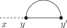
Figure 2: This diagram characterizes the partial topology of the mode function (88). The external leg denoted by a dashed line comes from the retarded Green’s function whereas the remaining part is the 2-point 1PI diagram.

In the preceding section we have derived the relation (90) between the quantum-corrected mode function and the canonical formalism. This also indicates that the expectation value of the commutator of the field and the creation operator has the same topology as the mode function [36]. The diagrammatic expression is depicted in Fig. 2. The main purpose of this section is to show that the mode function definition and the 2-point correlator definition share the same topology.

The diagram for the usual definition, the spatial Fourier transform of the 2-point correlator, looks like,

$$\!\int\!\!d^{3}xe^{i\vec{k}\cdot\vec{x}}\times\Bigl{(}\textrm{Fig.~{}1}\Bigr{)},$$ (91)

whereas the diagram for the $\Delta u(t,k)u^{*}(t,k)$ part of the mode function definition is,

$$\Bigl{(}\textrm{Fig.~{}2}\Bigr{)}\times u(y^{\prime 0},k)e^{i\vec{k}\cdot\vec{y^{\prime}}}\times u^{*}(t,k).$$ (92)

Note that the final three components in equation (92) can be re-written as,

$$e^{i\vec{k}\cdot\vec{y^{\prime}}}u(y^{\prime 0},k)u^{*}(t,k)\!=\!\!\int\!\!d^{3}x^{\prime}e^{i\vec{k}\cdot\vec{x^{\prime}}}i\Delta_{\scriptscriptstyle-+}(y^{\prime};x^{\prime}).$$ (93)

Actually each single propagator with different Schwinger-Keldysh polarity takes the form of the linear combination of $uu^{*}$ and $u^{*}u$ multiplying by a distinct theta function. Hence the mode function definition has the diagrammatic form,

$$\!\int\!\!d^{3}x^{\prime}e^{i\vec{k}\cdot\vec{x^{\prime}}}\times\Bigl{(}\textrm{Fig.~{}1}\Bigr{)}.$$ (94)

Therefore we conclude that the generic diagram topology of the mode function definition is identical to that of the correlator definition.

Appendix C Källen Representation

In this subsection we will point out the necessary conditions for Källen representation to hold through deriving it step by step. Although this familiar material has been covered in a textbook of quantum field theory, the purpose here is to remind readers that the familiar representation becomes nontrivial when applying it to FRW background in a theory without a mass gap.

In an interacting theory the 2-point correlation function is,

$$\Bigl{<}\Omega|\phi(x)\phi(y)|\Omega\Bigr{>}.$$ (95)

It is free to insert a partition of unity between the two field operators,

$$\textrm{I}=|\Omega\Bigr{>}\Bigl{<}\Omega|+\!\!\int\!\!\frac{d^{3}k}{(2\pi)^{3}}\frac{1}{2\omega}|k\Bigr{>}\Bigl{<}k|+\!\!\int\!\!\frac{d^{3}k_{1}}{(2\pi)^{3}}\frac{1}{2\omega_{1}}\!\!\int\!\!\frac{d^{3}k_{2}}{(2\pi)^{3}}\frac{1}{2\omega_{2}}|k_{1}k_{2}\Bigr{>}\Bigl{<}k_{1}k_{2}|+\cdots.\,$$ (96)

The 2-point correlation function (95) can be written as ,

$$\Bigl{<}\Omega|\phi(x)\phi(y)|\Omega\Bigr{>}=\Bigl{<}\Omega|\phi(x)|\Omega\Bigr{>}\Bigl{<}\Omega|\phi(y)|\Omega\Bigr{>}+\!\!\int\!\!\frac{d^{3}k}{(2\pi)^{3}}\frac{1}{2\omega}\Bigl{<}\Omega|\phi(x)|k\Bigr{>}\Bigl{<}k|\phi(y)|\Omega\Bigr{>}$$

$$\hskip 71.13188pt+\!\!\int\!\!\frac{d^{3}k_{1}}{(2\pi)^{3}}\frac{1}{2\omega_{1}}\!\!\int\!\!\frac{d^{3}k_{2}}{(2\pi)^{3}}\frac{1}{2\omega_{2}}\Bigl{<}\Omega|\phi(x)|k_{1}k_{2}\Bigr{>}\Bigl{<}k_{1}k_{2}|\phi(y)|\Omega\Bigr{>}+\cdots.$$ (97)

The first term of (97) can be subtracted from $\phi$ so the VEV of it is zero if the quantum field has been properly defined,

$$\Bigl{<}\Omega|\phi(x)|\Omega\Bigr{>}=\phi_{0},$$ (98)

and the resulting sum begins with the contribution from 1-particle states. Had a theory possessed poincaré symmetry, we can implement the following steps,

$$\Bigl{<}\Omega|\phi(x)|k\Bigr{>}=e^{-ik^{\mu}x_{\mu}}\Bigl{<}\Omega|\phi(0)|k\Bigr{>}=e^{-ik^{\mu}x_{\mu}}\Bigl{<}\Omega|\phi(0)|\vec{0}\Bigr{>}\equiv\sqrt{Z}e^{-ik^{\mu}x_{\mu}}.$$ (99)

The first equality is from the spacetime translation invariance of the 3-momentum state $|k\Bigr{>}$ and the vacuum $\Bigl{<}\Omega|$ whereas the second equality is due to the Lorentz boost invariance of $\phi(0)$ and the vacuum $\Bigl{<}\Omega|$. This is not a problem at all for a quantum field theory with a mass gap in a flat background. The first nonzero term of (97) is,

$$\int\!\!\frac{d^{3}k}{(2\pi)^{3}}\frac{1}{2\omega}Ze^{-ik^{\mu}(x-y)_{\mu}}=\!\int\!\!\frac{d^{4}k}{(2\pi)^{4}}\frac{iZe^{-ik^{\mu}(x-y)_{\mu}}}{k^{2}\!-\!m^{2}+i\epsilon}$$ (100)

Here we have assumed $x^{0}>y^{0}$ for convenience. Therefore we reach the familiar expression,

$$\Bigl{<}\Omega|\phi(x)\phi(y)|\Omega\Bigr{>}=\!\int\!\!\frac{d^{4}k}{(2\pi)^{4}}e^{-ik^{\mu}(x-y)_{\mu}}\Biggl{\{}\frac{iZ}{k^{2}\!-\!m^{2}+i\epsilon}+\sum\frac{iZ(\mu)}{k^{2}\!-\!\mu^{2}+i\epsilon}\Biggr{\}}.$$ (101)

The first term of (101) is the 1-particle contribution and the second term is the multi-particle continuation.

The primordial power spectrum is computed in FRW geometry which only possesses spatial rotation and spatial translation invariance rather than poincaré symmetry. Hence the 2-point correlation function is not able to reach the same expression as (101). As a result, there are no exact 1-particle states, nor even exact energy eigenstates. Nor is the VEV of the field zero, or even constant. Furthermore the graviton in FRW geometry experiences much more severe IR divergences than in flat background because a rapid spacetime expansion makes IR divergence much stronger. So it is also impossible to take the initial state back to a distant infinity and to define the unique vacuum as we did for a theory with a mass gap in flat spacetime.

Our toy model is in flat space background. However, because it is massless, $\varphi^{3}$ theory, the vacuum decays and it doesn’t have either time translation invariance or boost invariance [37]. It would indeed have an IR divergence if the computation had been done in 4-momentum space. However, in position space in the Schwinger-Keldysh (in-in) formalism there is no IR divergence as long as the state is released at a finite time. What we would instead get is a growth of the VEV of the field [38].

Based on the arguments being discussed in the preceding paragraphs, the mode function definition cannot recover the 1-particle states in källen representation either for quantum gravity in cosmology or for our toy model in flat spacetime. We also can see this from the diagram topology. The 1-particle contribution has infinite corrections from summing up a series of the 2-point correlator with more and more 1PI insertions as being shown in equation (7.43) of [39]. The topology of the mode function definition has been derived in equation (94) which shares the same topology as the spatial Fourier transform of the 2-point correlator. The two definitions both do not receive infinite corrections as the 1-particle states do. If the theory is poincaré invariant and has a mass gap, then we would get the same answer in both the in-out and in-in formalisms by taking the initial time to minus infinity. However, the subtle points the two definitions disagree at loop orders are that when there are particle productions (which there is for cosmology and for massless, $\varphi^{3}$ even in a flat space) and when we cannot take the initial time to minus infinity.

Appendix D The issues of divergences

In this subsection we renormalize the ultraviolet divergences of the two definitions in our toy model using a mass counterterm. For further clarification of the renormalized results we have emphasized the distinction between infrared divergences and secular growth. Finally, we discuss the extra, composite operator divergence which can occur in a model with derivative interactions, owing to the fact that the two times coincide.

D.1 The power spectrum from the mode function definition for $\varphi^{3}$ theory

Before computing the lowest order correction to the power spectrum from the mode function definition (18), we need to obtain the first order correction to the mode function using (37). Instead of employing the formal expression (38) and (46), the best way to get the finite result is to remove the ultraviolet divergence of the self-mass squared and then integrate the finite part against the tree order mode function. Even though the last step to solve for $\Delta u(t,k)$ from (37) still requires one more integral coming from the retarded Green’s function, it is actually not so hard to perform because it only involves with a temporal integration.

Recall that the primitive part of the one loop self-mass squared in $\varphi^{3}$ theory is,

$$-iM^{2}_{\scriptscriptstyle+\pm}(x;x^{\prime})=\mp\frac{\lambda^{2}}{2}\frac{\Gamma^{2}(\frac{D}{2}\!-\!1)}{16\pi^{D}}\frac{1}{\Delta x_{\scriptscriptstyle+\pm}^{2D-4}(x;x^{\prime})},$$ (102)

where $\Delta x^{2}_{\scriptscriptstyle+\pm}(x;x^{\prime})$ is defined in (27) and (28). Note that integrating expression (102) with respect to $x^{\prime\mu}$ in $D=4$ dimensions would produce a logarithmic divergence due to the singularity at $x^{\prime\mu}=x^{\mu}$. We can make the expression integrable by extracting a d’Alembertian with respect to $x^{\mu}$,

$$\int\!\!d^{4}x^{\prime}\frac{1}{\Delta x_{\scriptscriptstyle+\pm}^{2D-4}(x;x^{\prime})}=\frac{1}{2(D\!-\!3)(D\!-\!4)}\partial^{2}\!\!\int\!\!d^{4}x^{\prime}\frac{1}{\Delta x_{\scriptscriptstyle+\pm}^{2D-6}(x;x^{\prime})}.$$ (103)

The remaining obstacle to taking the $D\rightarrow 4$ limit is of course the explicit factor of $1/(D-4)$ in expression (103).

The next step is to segregate the divergence into a local delta function by adding zero in the form,

$$\partial^{2}\Bigl{[}\frac{1}{\Delta x^{D-2}_{\scriptscriptstyle++}}\Bigr{]}-\frac{i4\pi^{\frac{D}{2}}\delta^{D}(x\!-\!x^{\prime})}{\Gamma(\frac{D}{2}\!-\!1)}=0=\partial^{2}\Bigl{[}\frac{1}{\Delta x^{D-2}_{\scriptscriptstyle+-}}\Bigr{]}.$$ (104)

(For simplicity, we here and henceforth suppress the two arguments of the coordinate separation $\Delta x^{2}(x;x^{\prime})$.) We can then take the $D\rightarrow 4$ limit of the nonlocal part, leaving the divergence restricted to the delta function. For the $++$ case the result is,

$$\frac{1}{(D\!-\!4)}\Biggl{\{}\partial^{2}\Bigl{[}\frac{1}{\Delta x^{2D-6}_{\scriptscriptstyle++}}-\frac{\mu^{2D-4}}{\Delta x^{D-2}_{\scriptscriptstyle++}}\Bigr{]}+\frac{\mu^{D-4}i4\pi^{\frac{D}{2}}}{\Gamma(\frac{D}{2}\!-\!1)}\delta^{D}(x\!-\!x^{\prime})\Biggr{\}}$$ (105)

$$=\frac{\mu^{D-4}}{(D\!-\!4)}\frac{i4\pi^{\frac{D}{2}}}{\Gamma(\frac{D}{2}\!-\!1)}\delta^{D}(x\!-\!x^{\prime})-\frac{\partial^{2}}{2}\Biggl{[}\frac{\ln(\mu^{2}\Delta x^{2}_{\scriptscriptstyle++})}{\Delta x^{2}_{\scriptscriptstyle++}}\Biggr{]}+O(D\!-\!4).$$

At this point it is clear that the divergent part of the $++$ self-mass squared is,

$$\frac{-i\lambda^{2}}{2^{4}\pi^{\frac{D}{2}}}\frac{\Gamma(\frac{D}{2}\!-\!1)}{(D\!-\!3)}\frac{\mu^{D-4}}{(D\!-\!4)}\delta^{D}(x\!-\!x^{\prime}),$$ (106)

and it can be absorbed by a mass counterterm. Because there is no delta function for the $+-$ term in expression (104), the $+-$ self-mass squared has no ultraviolet divergence. This accords with the fact that the Schwinger-Keldysh formalism has no counterterms with mixed $\pm$ polarities [27, 28, 31].

It is simpler to perform the integral (37) by extracting one more d’Alembertian,

$$\Biggl{[}\frac{\ln(\mu^{2}\Delta x^{2}_{\scriptscriptstyle+\pm})}{\Delta x^{2}_{\scriptscriptstyle+\pm}}\Biggr{]}=\frac{\partial^{2}}{8}\Biggl{\{}\ln^{2}(\mu^{2}\Delta x^{2}_{\scriptscriptstyle+\pm})-2\ln(\mu^{2}\Delta x^{2}_{\scriptscriptstyle+\pm})\Biggr{\}}.$$ (107)

With the two simplifications,

$$\ln(\mu^{2}\Delta x^{2}_{\scriptscriptstyle+\pm})=\theta(t\!-\!t^{\prime})\theta(\Delta t\!-\!\Delta\overline{x})\Biggl{\{}\ln[\mu^{2}(\Delta t^{2}\!-\!\Delta\overline{x}^{2})]\pm i\pi\Biggr{\}},$$ (108)

the finite part can be written as,

$$M^{2}_{\scriptscriptstyle++}+M^{2}_{\scriptscriptstyle+-}=\frac{-\lambda^{2}}{2^{8}\pi^{3}}\partial^{4}\Biggl{\{}\theta(t\!-\!t^{\prime})\theta(\Delta t\!-\!\Delta\overline{x})\Biggl{(}\ln[\mu^{2}(\Delta t^{2}\!-\!\Delta\overline{x}^{2})]-1\Biggr{)}\Biggr{\}}.$$ (109)

Here $\Delta t^{2}$ and $\Delta\overline{x}^{2}$ are defined as $(t-t^{\prime})^{2}$ and $||\vec{x}-\vec{x^{\prime}}||^{2}$ respectively.

At this stage we are ready to integrate (109) against the tree order mode function,

$$\int\!\!d^{4}x^{\prime}\Bigl{[}M^{2}_{\scriptscriptstyle++}(x;x^{\prime})+M^{2}_{\scriptscriptstyle+-}(x;x^{\prime})\Bigr{]}u(t^{\prime},k)e^{i\vec{k}\cdot\vec{x^{\prime}}}$$

$$=\frac{-\lambda^{2}e^{i\vec{k}\cdot\vec{x}}}{2^{8}\pi^{3}}\partial^{4}\!\!\int_{0}^{t}\!dt^{\prime}\!\!\int_{0}^{\Delta t}\!\!drr^{2}d\Omega\Biggl{\{}\ln[\mu^{2}(\Delta t^{2}\!-\!\Delta\overline{x}^{2})]-1\Biggr{\}}\frac{e^{-ikt^{\prime}+i\vec{k}\cdot\vec{r}}}{\sqrt{2k}}.$$ (110)

Here we set $\vec{r}$ as $\vec{x^{\prime}}-\vec{x}$. After executing the angular integration and change the variable $r=|\vec{r}|=z\Delta t$, the expression can be simplified,

$$\frac{-\lambda^{2}}{2^{6}\pi^{2}}\frac{e^{i\vec{k}\cdot\vec{x}}}{k}(\partial_{0}^{2}\!+\!k^{2})^{2}\!\!\int_{0}^{t}\!\!dt^{\prime}\frac{e^{-ikt^{\prime}}}{\sqrt{2k}}\Delta t^{2}\!\!\int_{0}^{1}\!\!\!dzz\sin(kz\Delta t)\Biggl{\{}2\ln(\mu\Delta t)\!+\!\ln(1\!\!-\!z^{2})\!-\!1\Biggr{\}}\!.$$ (111)

To perform the $z$ integration we employ several special functions,

$$\textrm{Si}(x)\equiv-\!\!\int_{x}^{\infty}\!\!dt\frac{\sin(t)}{t}=-\frac{\pi}{2}+\!\!\int_{0}^{x}\!\!dt\frac{\sin(t)}{t};$$

$$\textrm{Ci}(x)\equiv-\!\!\int_{x}^{\infty}\!\!dt\frac{\cos(t)}{t}=\gamma+\ln(x)+\!\!\int_{0}^{x}\!\!dt\Biggl{[}\frac{\cos(t)\!-\!1}{t}\Biggr{]};$$

$$\xi(\alpha)\equiv\!\!\int_{0}^{1}\!dzz\sin(\alpha z)\ln(1\!-\!z^{2})=\frac{1}{\alpha^{2}}\Biggl{\{}2\sin(\alpha)\!-\!\Bigl{[}\cos(\alpha)\!+\!\alpha\sin(\alpha)\Bigr{]}\Bigl{[}\textrm{Si}(2\alpha)\!+\!\frac{\pi}{2}\Bigr{]}$$

$$\hskip 142.26378pt+\Bigl{[}\sin(\alpha)\!-\!\alpha\cos(\alpha)\Bigr{]}\Bigl{[}\textrm{Ci}(2\alpha)\!-\!\gamma\!-\!\ln(\frac{\alpha}{2})\Bigr{]}\Biggr{\}}.$$ (112)

With these the renormalized result can be expressed as,

$$\frac{-\lambda^{2}}{2^{6}\pi^{2}}\frac{e^{i\vec{k}\cdot\vec{x}}}{k^{3}}(\partial_{0}^{2}\!+\!k^{2})^{2}\!\!\int_{0}^{t}\!\!dt^{\prime}\frac{e^{-ikt^{\prime}}}{\sqrt{2k}}\Biggl{\{}\!\alpha^{2}\xi(\alpha)\!+\!\Bigl{[}2\ln(\frac{\mu\alpha}{k})\!-\!1\Bigr{]}\Bigl{[}\sin(\alpha)\!-\!\alpha\cos(\alpha)\Bigr{]}\!\Biggr{\}}\!.$$ (113)

Here $\alpha$ is $k\Delta t$.

Because the integrand of (113) behaves like $\Delta t^{3}\ln(\Delta t)$ near $t^{\prime}\!=\!t$ we can pass three of four derivatives through the integral sign to simplify the integrand. Passing the first two derivatives through gives,

$$\frac{-\lambda^{2}}{2^{5}\pi^{2}}\frac{e^{i\vec{k}\cdot\vec{x}}}{k}(\partial_{0}\!+\!ik)(\partial_{0}\!-\!ik)\!\!\int_{0}^{t}\!\!dt^{\prime}\frac{e^{-ikt^{\prime}}}{\sqrt{2k}}\Biggl{\{}\!-\cos(\alpha)\!\!\int_{0}^{2\alpha}\!\!ds\frac{\sin(s)}{s}$$

$$\hskip 105.2751pt+\sin(\alpha)\Biggl{[}\int_{0}^{2\alpha}\!\!ds\frac{\cos(s)\!-\!1}{s}\!+\!2\ln(\frac{2\mu\alpha}{k})\Biggr{]}\Biggr{\}}.$$ (114)

Extracting the temporal phase factor and passing one more derivative through the integral gives,

$$\frac{-\lambda^{2}}{2^{5}\pi^{2}}e^{i\vec{k}\cdot\vec{x}}(\partial_{0}\!+\!ik)\!\!\int_{0}^{t}\!\!dt^{\prime}\frac{e^{-ikt^{\prime}}}{\sqrt{2k}}e^{-ik\Delta t}\Biggl{[}\!\int_{0}^{2\alpha}\!\!ds\frac{e^{is}-1}{s}\!+\!2\ln(2\mu\Delta t)\Biggr{]}$$

$$=\frac{-\lambda^{2}}{2^{5}\pi^{2}}\frac{e^{-ikt+i\vec{k}\cdot\vec{x}}}{\sqrt{2k}}\partial_{0}\!\int_{0}^{t}\!\!d\Delta t\times 1\times\Biggl{\{}\Biggl{[}\!\int_{0}^{2k\Delta t}\!\!ds\frac{e^{is}-1}{s}\Biggr{]}\!+\!2\ln(2\mu\Delta t)\Biggr{\}}.$$ (115)

Here we have used $(\partial_{0}+ik)e^{-ikt}=0$. Further simplification can be accomplished by performing the $\Delta t$ integration and acting the final derivative. The final result is,

$$\frac{-\lambda^{2}}{2^{5}\pi^{2}}\frac{e^{-ikt+i\vec{k}\cdot\vec{x}}}{\sqrt{2k}}\Biggl{\{}\!\int_{0}^{2kt}\!\!ds\frac{e^{is}-1}{s}\!+\!2\ln(2\mu t)\Biggr{\}}\equiv-S(t)e^{i\vec{k}\cdot\vec{x}}.$$ (116)

According to (37) the $\Delta u(t,k)$ we want to solve for obeys,

$$\mathcal{D}\Bigl{[}\Delta u(t,k)e^{i\vec{k}\cdot\vec{x}}\Bigr{]}\!=\!-(\partial_{0}^{2}\!+\!k^{2})\Delta u(t,k)e^{i\vec{k}\cdot\vec{x}}\!=\!-S(t)e^{i\vec{k}\cdot\vec{x}}\,\,\,\Longrightarrow$$

$$(\partial_{0}^{2}\!+\!k^{2})\Delta u(t,k)\!=\!S(t)\,\,\Longrightarrow\,\,\Delta u(t,k)\!=\!\!\int_{0}^{\infty}\!\!dt^{\prime}G_{r}(t,t^{\prime})S(t^{\prime}).$$ (117)

Here $G_{r}(t,t^{\prime})=\theta(t\!-\!t^{\prime})\frac{\sin(k\Delta t)}{k}$ is the retarded Green’s function. Plugging the explicit forms of $G_{r}(t,t^{\prime})$ and $S(t^{\prime})$ into (117) gives,

$$\Delta u(t,k)\!=\!\frac{\lambda^{2}}{2^{5}\pi^{2}}\frac{e^{-ikt}}{i(2k)^{\frac{3}{2}}}\!\int_{0}^{t}\!\!dt^{\prime}\Bigl{\{}e^{2ik\Delta t}\!-\!1\Bigr{\}}\Biggl{\{}\!\int_{0}^{2kt^{\prime}}\!\!ds\frac{e^{is}-1}{s}\!+\!2\ln(2\mu t^{\prime})\Biggr{\}}.$$ (118)

It remains to perform the four $t^{\prime}$ integrations and collect terms. The result is,

$$\Delta u(t,k)\!=\!\frac{\lambda^{2}}{2^{5}\pi^{2}}\frac{e^{-ikt}}{(2k)^{\frac{3}{2}}}\Biggl{\{}\!\Biggl{[}\frac{1}{2k}\!+\!it\Biggr{]}\!\int_{0}^{2kt}\!\!ds\frac{e^{is}\!-\!1}{s}\!-\!\frac{e^{2ikt}}{2k}\!\!\int_{0}^{2kt}\!\!ds\frac{e^{-is}\!-\!1}{s}$$

$$\hskip 85.35826pt+\Biggl{[}\frac{1\!-\!e^{2ikt}}{k}\!+\!2it\Biggr{]}\ln(2\mu t)\!-\!it\!+\!\frac{1\!-\!e^{2ikt}}{2k}\Biggr{\}}.$$ (119)

Combining (119)$\times[u^{*}(t,k)=\frac{e^{-ikt}}{\sqrt{2k}}]$ with its complex conjugate gives the lowest-order correction to the power spectrum,

$$\Delta u(t,k)u^{*}(t,k)\!+\!\textrm{c.c.}\!=\!\frac{\lambda^{2}}{2^{7}\pi^{2}}\frac{1}{k^{3}}\Biggl{\{}\Bigl{[}1\!-\!\cos(2kt)\Bigr{]}\Bigl{[}1\!-\!\gamma\!+\!\textrm{Ci}(2kt)\!+\!\ln(\frac{2\mu^{2}t}{k})\Bigr{]}$$

$$\hskip 142.26378pt-\Bigl{[}\sin(2kt)\!+\!2kt\Bigr{]}\Bigl{[}\frac{\pi}{2}\!+\!\textrm{Si}(2kt)\Bigr{]}\Biggr{\}}.$$ (120)

D.2 The power spectrum from the correlator definition for $\varphi^{3}$ theory

We begin by removing the ultraviolet divergence of the self-mass squared embedded in the 2-point correlator using the same procedure prescribed in the previous subsection. We also perform two partial integrations and carry out the spatial Fourier transforms.

Even though the 2-point correlator carries various polarities on the self-mass squared and the external legs (Fig.1), we suppress the polarities and the relative signs in order to investigate the generic pattern ,

$$\frac{-\lambda^{2}}{2}\Biggl{[}\frac{\Gamma(\frac{D}{2}\!-\!1)}{4\pi^{\frac{D}{2}}}\Biggr{]}^{4}\!\!\int\!\!d^{D}y\frac{1}{\Delta x^{\scriptscriptstyle D-2}(x;y)}\!\!\int\!\!d^{D}y^{\prime}\frac{1}{\Delta x^{\scriptscriptstyle 2D-4}(y;y^{\prime})}\frac{1}{\Delta x^{\scriptscriptstyle D-2}(x^{\prime};y^{\prime})},$$

$$\Longrightarrow\frac{-\lambda^{2}}{2}\frac{1}{2^{8}\pi^{8}}\!\!\int\!\!d^{4}y\frac{1}{\Delta x^{\scriptscriptstyle 2}(x;y)}\!\!\times\!\!\frac{-1}{4}\!\!\int\!\!d^{4}y^{\prime}\partial_{y}^{2}\Biggl{[}\frac{\ln[\mu^{\scriptscriptstyle 2}\Delta x^{\scriptscriptstyle 2}(y;y^{\prime})]}{\Delta x^{\scriptscriptstyle 2}(y;y^{\prime})}\Biggr{]}\frac{1}{\Delta x^{\scriptscriptstyle 2}(x^{\prime};y^{\prime})}.$$ (121)

To reach the second line, we have employed (103) to make the function integrable with respect to $y^{\prime\mu}$ in $D=4$ dimensions. We then segregated the ultraviolet divergence into a local delta function using (104) and absorbed it with a mass counterterm, just as in the previous subsection.

Because the derivative only acts on a function of the coordinate separation, we can replace $\partial^{2}_{y}$ with $\partial^{2}_{y^{\prime}}$ and then partially integrate to reach the form,

$$\frac{\ln[\mu^{\scriptscriptstyle 2}\Delta x^{\scriptscriptstyle 2}(y;y^{\prime})]}{\Delta x^{\scriptscriptstyle 2}(y;y^{\prime})}\Biggl{[}\partial_{y}^{\prime 2}\frac{1}{\Delta x^{\scriptscriptstyle 2}(x^{\prime};y^{\prime})}\Biggr{]}\!+\!\textrm{two surface terms}.$$ (122)

After dropping the surface terms, the $y^{\prime}$ integration can be carried out using (104),

$$\frac{i\lambda^{2}}{2^{9}\pi^{6}}\!\!\int\!\!d^{4}y\frac{1}{\Delta x^{\scriptscriptstyle 2}(x;y)}\frac{\ln[\mu^{\scriptscriptstyle 2}\Delta x^{\scriptscriptstyle 2}(y;x^{\prime})]}{\Delta x^{\scriptscriptstyle 2}(y;x^{\prime})}.$$ (123)

Note that only the first and third diagrams of Fig.1 survive because their right external legs carry the same polarity.

Further reduction can be accomplished by extracting another d’Alembertian using (107), performing a partial integration and then carrying out the $y$ integration,

$$\frac{\lambda^{2}}{2^{10}\pi^{4}}\Biggl{\{}\ln^{2}[\mu^{\scriptscriptstyle 2}\Delta x^{\scriptscriptstyle 2}_{\scriptscriptstyle-+}(x;x^{\prime})]\!-\!2\ln(\mu^{\scriptscriptstyle 2}\Delta x^{\scriptscriptstyle 2}_{\scriptscriptstyle-+}(x;x^{\prime})]\Biggr{\}}\!+\!\textrm{two surface terms}.$$ (124)

It is clear that the final survival term is from the third diagram of Fig.1 because its two external legs carry the same polarity. Because $x^{\mu}\!=\!(t,\vec{x})$ and $x^{\prime\mu}\!=\!(t,\vec{0})$ have the same time components, the coordinate separation $\Delta x^{2}(x;x^{\prime})$ in (124) is purely spatial. The spatial Fourier transform of (124) can be easily performed to give,

$$\frac{\lambda^{2}}{2^{10}\pi^{4}}\!\!\int\!\!d^{3}xe^{-i\vec{k\cdot\vec{x}}}\Biggl{\{}\!\ln^{2}[\mu^{\scriptscriptstyle 2}|\vec{x}|^{\scriptscriptstyle 2}]\!-\!2\ln[\mu^{\scriptscriptstyle 2}|\vec{x}|^{\scriptscriptstyle 2}]\!\Biggr{\}}\!=\!\frac{\lambda^{2}}{2^{10}\pi^{4}}\frac{4^{2}\pi}{k}\!\!\int_{0}^{\infty}\!\!drr\sin(kr)\Big{\{}\!\ln^{2}[\mu r]\!-\!\ln[\mu r]\!\Bigr{\}}$$

$$=\frac{\lambda^{2}k^{-1}}{2^{6}\pi^{3}}\frac{-\partial}{\partial k}\!\!\int_{0}^{\infty}\!\!dr\cos(kr)\Biggl{\{}\ln^{2}[\mu r]\!-\!\ln[\mu r]\Biggr{\}}\!=\!\frac{\lambda^{2}k^{-1}}{2^{6}\pi^{3}}\frac{-\partial}{\partial k}\Biggl{\{}\frac{\pi}{k}\Bigl{[}\frac{1}{2}\!+\!\gamma\!-\!\ln(\frac{\mu}{k})\Bigr{]}\Biggr{\}}.$$ (125)

Two special integrals [40] have been employed in the last equality,

$$\int_{0}^{\infty}\!\!dz\frac{\sin(z)}{z}\!=\!\frac{\pi}{2}\,\,\,;\,\,\,\!\!\int_{0}^{\infty}\!\!dz\frac{\sin(z)}{z}\ln(z)\!=\!\frac{\pi}{2}\gamma,\,\,\,\,\,\gamma\equiv\textrm{Euler's constant}.$$ (126)

The lowest correction to the power spectrum by the correlator definition is therefore,

$$\int\!\!d^{3}xe^{-i\vec{k\cdot\vec{x}}}\Bigl{<}\Omega|\varphi(t,\vec{x})\varphi(t,\vec{0})|\Omega\Bigr{>}_{\scriptstyle 1\,loop}\!=\!\frac{\lambda^{2}}{2^{6}\pi^{2}}\frac{1}{k^{3}}\Bigl{\{}\frac{1}{2}\!+\!\gamma\!-\!\ln(\frac{\mu}{k})\Bigr{\}}.$$ (127)

D.3 Discussions of infrared and ultraviolet divergences

There is an unfortunate tendency in the literature to employ the term “infrared divergence” to describe perfectly finite, temporally growing effects such as (120). Of course a true infrared divergence is an infinite constant, with no spacetime dependence. That neither definition for the power spectrum can give rise to an infrared divergence is a simple consequence of the Schwinger-Keldysh formalism with the initial states being released at finite times. In order to produce a true infrared divergence, interactions must contribute from arbitrarily large spatial distances, and this is precluded by causality as long as the initial state is released at any finite time.

Ultraviolet divergences can and do occur in the Schwinger-Keldysh formalism, just as they do in the in-out formalism. In both formalisms it is important to distinguish between the ultraviolet divergences of non-coincident 1PI functions, which are eliminated by conventional BPHZ renormalization, and the new divergences which can occur when one or more of the coordinates are related. These new divergences require an extra, composite operator renormalization. The case of the power spectrum is especially tricky because only the time components of the two spacetime points are made to coincide. For the case of our toy $\varphi^{3}$ model, this produces no extra divergence. The vertices of quantum gravity contain derivatives, which increases the tendency for divergences. Frob, Roura and Verdaguer have claimed that this is enough to cause the one loop correction to the correlator definition of the power spectrum to harbor a new, composite operator divergence. One of our points is that the mode function definition is free from this new divergence.

References

- [1] A. A. Starobinsky, JETP Lett. 30 (1979) 682.
- [2] V. F. Mukhanov and G. V. Chibisov, JETP Lett. 33 (1981) 532.
- [3] G. F. Smoot, C. L. Bennett, A. Kogut, E. L. Wright, J. Aymon, N. W. Boggess, E. S. Cheng and G. De Amici et al., Astrophys. J. 396 (1992) L1-L5
- [4] E. Komatsu et al., Astrophys. J. Suppl. 192 (2011) 18, arXiv:1001.4538; G. Hinshaw et al., Astrophys. J. Suppl. 208 (2013) 19, arXiv:1212.5226.
- [5] P. A. R. Ade et al., arXiv:1303.5076 .
- [6] Z. Hou, C. L. Reichardt, K. T. Story, B. Follin, R. Keisler, K. A. Aird, B.A. Benson and L.E. Bleem et al., arXiv:1212.6267.
- [7] J. L. Sievers, R. A. Hlozek, M. R. Nolta, V. Acquaviva, G. E. Addison, P. A. R. Ade, P. Aguirre and M. Amiri et al., arXiv:1301.0824; S. Das, T. Louis, M. R. Nolta, G. E. Addison, E. S. Battistelli, J. R. Bond, E. Calabrese and D. C. M. J. Devlin et al., arXiv:1301.1037.
- [8] E. O. Kahya, V. K. Onemli and R. P. Woodard, Phys. Lett. B694 (2010) 101, arXiv:1006.3999.
- [9] S. R. Furlanetto, S. P. Oh and F. H. Briggs, Phys. Rept. 433 (2006) 181, astro-ph/0608032.
- [10] T. C. Chang, U. L. Pen, K. Bandura and J. B. Peterson, Nature 466 (2010) 463, arXiv:1007.3709.
- [11] S. Weinberg, Phys. Rev. D72 (2005) 043514, hep-th/0506236; Phys. Rev. D74 (2006) 023508, hep-th/0605244.
- [12] J. Serreau, arXiv:1302.6365; J. Serreau and R. Parentani, Phys. Rev. D 87 (2013) 085012, arXiv:1302.3262; K. Larjo and D. A. Lowe, arXiv:1301.4274; K. Feng, Y.-F. Cai and Y.-S. Piao, Phys. Rev. D 86 (2012) 103515, arXiv:1207.4405; D. Boyanovsky, Phys. Rev. D 86 (2012) 023509, arXiv:1205.3761, Phys. Rev. D 85 (2012) 123525, arXiv:1203.3903; H. Kitamoto and Y. Kitazawa, Phys. Rev. D 87 (2013) 124004, arXiv:1204.2876, Phys. Rev. D 85 (2012) 044062, arXiv:1109.4892, Phys. Rev. D 83 (2011) 104043, arXiv:1012.5930; J.-T. Hsiang, C.-H. Wu, L.H. Ford and K.-W. Ng, Phys. Rev. D 84 (2011) 103515, arXiv:1105.1155; D. Chialva and A. Mazumdar, arXiv:1103.1312; M. Gerstenlauer, A. Hebecker and G. Tasinato, JCAP 1106 (2011) 021, arXiv:1102.0560; J.-T. Hsiang, L. H. Ford, D.-S. Lee and H.-L. Yu, Phys. Rev. D 83 (2011) 084027, arXiv:1012.1582; N. Bartolo, E. Dimastrogiovanni and A. Vallinotto, JCAP 1011 (2010) 003, arXiv:1006.0196; L. H. Ford, S. P. Miao, K.-W. Ng, R. P. Woodard and C.-H.Wu, Phys. Rev.D 82 (2010) 043501,arXiv:1005.4530; C. P. Burgess, R. Holman, L. Leblond and S. Shandera, JCAP 1010 (2010) 017, arXiv:1005.3551; X. Gao and F. Xu, JCAP 0907 (2009) 042, arXiv:0905.0405; E. Dimastrogiovanni and N. Bartolo, JCAP 0811 (2008) 016, arXiv:0807.2790.
- [13] D. Seery, J. E. Lidsey and M. S. Sloth, JCAP 0701 (2007) 027, astro-ph/0610210.
- [14] P. R. Jarnhus and M. S. Sloth, JCAP 0802 (2008) 013, arXiv:0709.2708.
- [15] W. Xue, X. Gao and R. Brandenberger, JCAP 1206 (2012) 035, arXiv:1201.0768.
- [16] D. Boyanovsky, H. J. de Vega and N. G. Sanchez, Nucl. Phys. B747 (2006) 25, astro-ph/0503669; Phys. Rev. D72 (2005) 103006, astro-ph/0507596; M. Sloth, Nucl. Phys. B748 (2006) 149, astro-ph/0604488; Nucl. Phys. B775 (2007) 78, hep-th/0612138; A. Bilandžić and T. Prokopec, Phys. Rev. D76 (2007) 103507, arXiv:0704.1905; M. van der Meulen and J. Smit, JCAP 0711 (2007) 023, arXiv:0707.0842; D. H. Lyth, JCAP 0712 (2007) 016, arXiv:0707.0361; D. Seery, JCAP 0711 (2007) 025, arXiv:0707.3377; JCAP 0802 (2008) 006, arXiv:0707.3378; JCAP 0905 (2009) 021, arXiv:0903.2788; N. Bartolo, S. Matarrese, M. Pietroni, A. Riotto and D. Seery, JCAP 0801 (2008) 015, arXiv:0711.4263, Y. Urakawa and K. I Maeda, Phys. Rev. D78 (2008) 064004, arXiv:0801.0126, A. Riotto and M. Sloth, JCAP 0804 (2008) 030, arXiv:0801.1845, K. Enqvist, S. Nurmi, D. Podolsky and G. I. Rigopoulos, JCAP 0804 (2008) 025, arXiv:0802.0395, P. Adshead, R. Easther and E. A. Lim, Phys. Rev. D79 (2009) 063504, arXiv:0809.4008, J. Kumar, L. Leblond and A. Rajaraman, JCAP 1004 (2010) 024, arXiv:0909.2040; C. P. Burgess, R. Holman, L. Leblond and S. Shandera, JCAP 1003 (2010) 033, arXiv:0912.1608, L. Senatore and M. Zaldarriaga, JHEP 1012 (2010) 008, arXiv:0912.2734; arXiv:1203.6354; arXiv:1203.6884, D. Seery, Class. Quant. Grav. 27 (2010) 124005, arXiv:1005.1649, G. L. Pimental, L. Senatore and M. Zaldarriaga, arXiv:1203.6651.
- [17] S. B. Giddings and M. S. Sloth, JCAP 1101 (2011) 023, arXiv:1005.1056; JCAP 1007 (2010) 015, arXiv:1005.3287; Phys. Rev. D84 (2011) 063528, arXiv:1104.0002; arXiv:1109.1000.
- [18] Y. Urakawa and T. Tanaka, arXiv:1209.1914, arXiv:1301.3088, Prog. Theor. Phys. 122 (2009) 779, arXiv:0902.3209, Prog. Theor. Phys. 122 (2009) 1207, arXiv:0904.4415; Phys. Rev. D82 (2010) 121301, arXiv:1007.0468; Prog. Theor. Phys. 125 (2011) 1067, arXiv:1009.2947; JCAP 1105 (2011) 014, arXiv:1103.1251; C. T. Byrnes, M. Gerstenlauer, A. Hebecker, S. Nurmi and G. Tasinato, JCAP 1008 (2010) 006, arXiv:1005.3307, M. Gerstenlauer, A. Hebecker and G. Tasinato, JCAP 1106 (2011) 021, arXiv:1102.0560; Y. Urakawa, Prog. Theor. Phys. 126 (2011) 961, arXiv:1105.1078; D. Chialva and A. Mazumdar, arXiv:1103.1312.
- [19] S. P. Miao and R. P. Woodard, JCAP 1207 (2012) 008, arXiv:1204.1784.
- [20] J. Maldacena, JHEP 0305 (2003) 013, astro-ph/0210603.
- [21] S. Weinberg, Phys. Rev. D72 (2005) 043514, hep-th/0506236; Phys. Rev. D74 (2006) 023508, hep-th/0605244.
- [22] R. Arnowitt, S. Deser and C. W. Misner, Phys. Rev. 116 (1959) 1322; Phys. Rev. 117 (1960) 1595; Nuov. Cim. 15 (1960) 487; Phys. Rev. 118 (1960) 1100; J. Math. Phys. 1 (1960) 434; Phys. Rev. 120 (1960) 313; 321; Phys. Rev. 120 (1960) 321; Ann. Phys. 11 (1960) 116; Nuov. Cim. 19 (1961) 668; Phys. Rev. 121 (1961) 1556; Phys. Rev. 122 (1961) 997; gr-qc/0405109.
- [23] J. Schwinger, J. Math. Phys. 2 (1961) 407.
- [24] K. T. Mahanthappa, Phys. Rev. 126 (1962) 329.
- [25] P. M. Bakshi, K. T. Mahanthappa, J. Math. Phys. 4 (1963) 1; J. Math. Phys. 4 (1963) 12.
- [26] L. V. Keldysh, Sov. Phys. JETP 20 (1965) 1018.
- [27] K. C. Chou, Z. B. Su, B. L. Hao, L. Yu, Phys. Rept. 118 (1985) 1.
- [28] R. D. Jordan, Phys. Rev. D33 (1986) 444.
- [29] E. Calzetta, B. L. Hu, Phys. Rev. D35 (1987) 495.
- [30] S. P. Miao, arXiv:0705.0767.
- [31] L. H. Ford, R. P. Woodard, Class. Quant. Grav. 22 (2005) 1637, gr-qc/0411003.
- [32] T. Brunier, V. K. Onemli and R. P. Woodard, Class. Quant. Grav. 22 (2005) 59, gr-qc/0408080.
- [33] M. B. Fröb, A. Roura and E. Verdaguer, JCAP 1208 (2012) 009, arXiv:1205.3097.
- [34] B. L. Hu, A. Roura and E. Verdaguer, Phys. Rev. D 70 (2004) 044002, [gr-qc/0402029].
- [35] R. K. Sachs and A. M.Wolfe, Astrophys. J. 147 (1967) 73, [Gen. Rel. Grav. 39 (2007) 1929]
- [36] S. P. Miao and R. P.Woodard, Phys. Rev. D 74 (2006) 024021, gr-qc/0603135.
- [37] G. Veneziano, Nucl. Phys. B 44 (1972), 142.
- [38] N. C. Tsamis and R. P. Woodard, Annals Phys. 238 (1995), 1.
- [39] An Introduction to Quantum Field Theory, Michael E. Peskin and Daniel V. Schroeder, Addison-Wesley, Cambridge, 1995.
- [40] Tabels of integrals, series, and Products, I.S. Gradsbteyn and I.M. Ryzbik, sixtrh edition, Academic Press, San Diego, 2000, 3.721-1(p417) and 4.421-1(p590).