Parallel Coordinate Descent Newton Method
for Efficient L1subscript𝐿1L_{1}-Regularized Loss Minimization††thanks: Source code is available at https://github.com/bianan/ParallelCDN

An Bian
ybian@inf.ethz.ch
ETH Zurich
&Xiong Li
li.xiong@gmail.com
CNCERT
\ANDYuncai Liu
whomliu@sjtu.edu.cn
Shanghai Jiao Tong University
&Ming-Hsuan Yang
mhyang@ucmerced.edu
University of California, Merced
Abstract

The recent years have witnessed advances in parallel algorithms for large scale optimization problems. Notwithstanding the demonstrated success, existing algorithms that parallelize over features are usually limited by divergence issues under high parallelism or require data preprocessing to alleviate these problems. In this work, we propose a Parallel Coordinate Descent algorithm using approximate Newton steps (PCDN) that is guaranteed to converge globally without data preprocessing. The key component of the PCDN algorithm is the high-dimensional line search, which guarantees the global convergence with high parallelism. The PCDN algorithm randomly partitions the feature set into b𝑏b subsets/bundles of size P𝑃P, and sequentially processes each bundle by first computing the descent directions for each feature in parallel and then conducting P𝑃P-dimensional line search to compute the step size. We show that (i) the PCDN algorithm is guaranteed to converge globally despite increasing parallelism; (ii) the PCDN algorithm converges to the specified accuracy Ο΅italic-Ο΅\epsilon within the limited iteration number of TΟ΅subscript𝑇italic-Ο΅T_{\epsilon}, and TΟ΅subscript𝑇italic-Ο΅T_{\epsilon} decreases with increasing parallelism. In addition, the data transfer and synchronization cost of the P𝑃P-dimensional line search can be minimized by maintaining intermediate quantities. For concreteness, the proposed PCDN algorithm is applied to L1subscript𝐿1L_{1}-regularized logistic regression and L1subscript𝐿1L_{1}-regularized L2subscript𝐿2L_{2}-loss SVM problems. Experimental evaluations on seven benchmark datasets show that the proposed PCDN algorithm exploits parallelism well and outperforms the state-of-the-art methods.

1 Introduction

High dimensional L1subscript𝐿1L_{1}-minimization problems arise in a wide range of applications including sparse logistic regression [15], L1subscript𝐿1L_{1}-regularized support vector machine (SVM) classification [4], image coding [11], and face recognition [23]. To solve L1subscript𝐿1L_{1}-optimization problems efficiently, several algorithms based on coordinate gradient descent (CGD) [22], stochastic gradient [21], interior point [8] and trust region [12] have been developed, among which the Coordinate Descent Newton (CDN) [24] and improved GLMNET [25] methods have demonstrated promising results for L1subscript𝐿1L_{1}-regularized linear optimization problems.

Within the L1subscript𝐿1L_{1}-optimization framework, large datasets with high dimensional features entail scalable and efficient parallel algorithms. Several methods perform parallelization over samples [9; 26; 27; 16] although usually there are more features than samples in L1subscript𝐿1L_{1}-regularized problems. RichtÑrik et al. [17] show that randomized coordinate descent methods can be accelerated by parallelization for solving Lasso problems, and the work is further extended to distributed settings [14; 18]. In addition, Bradley et al. [2] propose the Shotgun CDN (SCDN) method for L1subscript𝐿1L_{1}-regularized logistic regression by directly parallelizing the updates of features based on the CDN algorithm [24]. However, the SCDN method is not guaranteed to converge when the number of updated features in parallel is greater than a threshold, and thereby limits its ability of exploiting high parallelism. While this problem can be alleviated by preprocessing samples (e.g., feature clustering) to achieve higher parallelism [20], it requires additional computational overhead. The Accelerated Shotgun method [13] is a first-order algorithm without backtrack line search which has fast convergence. However, it can only deal with the objective functions without regularization terms. Scherrer et al. [19] present a generic framework for parallel coordinate descent methods which includes Shotgun, Greedy, Thread-Greedy and Coloring. Their empirical convergence and scalability tests do not favor any of these methods over the others, and no theoretical analysis is presented for the general framework.

In [1] Bian et al. present a high dimensional line search algorithm to ensure global convergence while performing parallel coordinate updates for L1subscript𝐿1L_{1}-regularized logistic regression problem. While this method performs well, no analysis of convergence rate is presented. In this work, by further exploring the idea, we propose a generalized Parallel Coordinate Descent method using approximate Newton steps (PCDN) for generic L1subscript𝐿1L_{1}-optimization problems, and present thorough theoretical analysis on the proposed method.

The contributions and novelty of this work are summarized as follows. We present theoretical analysis on the upper bound of the expected line search step in each iteration. We analyze the iteration complexity of the proposed PCDN algorithm and show that, for any bundle size P𝑃P (i.e., parallelism), it is guaranteed to converge to a specified accuracy Ο΅italic-Ο΅\epsilon within TΟ΅subscript𝑇italic-Ο΅T_{\epsilon} iterations. The iteration number TΟ΅subscript𝑇italic-Ο΅T_{\epsilon} decreases with the increasing of parallelism (bundle size P𝑃P). In addition, we show that in our implementation, the P𝑃P-dimensional line search does not need to access all the training data on each thread and the synchronization cost of the P𝑃P-dimensional line search can be minimized. Extensive experiments on L1subscript𝐿1L_{1}-regularized classification and regression problems with real-world datasets demonstrate that the proposed PCDN algorithm is a highly parallelized approach with guaranteed global convergence and fast convergence rate.

2 L1subscript𝐿1L_{1}-Regularized Loss Minimization

For ease of presentation, we summarize the mathematical notations in TableΒ 1.

Table 1: Mathematical notations in this work.
s𝑠s, n𝑛n # training samples and # features
i𝑖i, j𝑗j sample index and feature index
t𝑑t cumulative inner iteration index
kπ‘˜k outer iteration index
𝐞jsubscriptπžπ‘—\mathbf{e}_{j} indicator vector
βˆ₯β‹…βˆ₯\|\cdot\|, βˆ₯β‹…βˆ₯1\|\cdot\|_{1} 222-norm and 111-norm
𝒩𝒩\mathcal{N} {1,2,…,n}12…𝑛\{1,2,...,n\}, feature index set
β„¬βŠ†π’©β„¬π’©\mathcal{B}\subseteq\mathcal{N} feature index subset or β€œbundle”
P=|ℬ|𝑃ℬP=|\mathcal{B}| bundle size
π°βˆˆβ„n𝐰superscriptℝ𝑛\mathbf{w}\in\mathbb{R}^{n} unknown vector of model weights
π—βˆˆβ„sΓ—n𝐗superscriptℝ𝑠𝑛\mathbf{X}\in\mathbb{R}^{s\times n} design matrix, whose i𝑖i-th row is 𝐱isubscript𝐱𝑖\mathbf{x}_{i}
(𝐱i,yi)subscript𝐱𝑖subscript𝑦𝑖(\mathbf{x}_{i},y_{i}) sample-label pair

Consider an unconstrained L1subscript𝐿1L_{1}-regularized minimization problem over a training set {(𝐱i,yi)}i=1ssuperscriptsubscriptsubscript𝐱𝑖subscript𝑦𝑖𝑖1𝑠\{(\mathbf{x}_{i},y_{i})\}_{i=1}^{s} with the following general form:

minπ°βˆˆβ„n⁑F​(𝐰):=minπ°βˆˆβ„n⁑cβ€‹βˆ‘i=1sφ​(𝐰;𝐱i,yi)+‖𝐰‖1=minπ°βˆˆβ„n⁑L​(𝐰)+‖𝐰‖1,assignsubscript𝐰superscriptℝ𝑛𝐹𝐰subscript𝐰superscriptℝ𝑛𝑐superscriptsubscript𝑖1π‘ πœ‘π°subscript𝐱𝑖subscript𝑦𝑖subscriptdelimited-βˆ₯βˆ₯𝐰1subscript𝐰superscriptℝ𝑛𝐿𝐰subscriptdelimited-βˆ₯βˆ₯𝐰1\begin{split}\min_{\mathbf{w}\in\mathbb{R}^{n}}F(\mathbf{w})&:=\min_{\mathbf{w}\in\mathbb{R}^{n}}c\sum_{i=1}^{s}\varphi(\mathbf{w};\mathbf{x}_{i},y_{i})+\|\mathbf{w}\|_{1}\\ &=\min_{\mathbf{w}\in\mathbb{R}^{n}}L(\mathbf{w})+\|\mathbf{w}\|_{1},\end{split} (1)

where L​(𝐰):=cβ€‹βˆ‘i=1sφ​(𝐰;𝐱i,yi)assign𝐿𝐰𝑐superscriptsubscript𝑖1π‘ πœ‘π°subscript𝐱𝑖subscript𝑦𝑖L(\mathbf{w}):=c\sum_{i=1}^{s}\varphi(\mathbf{w};\mathbf{x}_{i},y_{i}) is the overall loss function; φ​(𝐰;𝐱i,yi)πœ‘π°subscript𝐱𝑖subscript𝑦𝑖\varphi(\mathbf{w};\mathbf{x}_{i},y_{i}) is a convex and non-negative loss function; and c>0𝑐0c>0 is the regularization parameter. For L1subscript𝐿1L_{1}-regularized logistic regression, the loss function is,

Ο†log​(𝐰;𝐱i,yi)=log⁑(1+eβˆ’yiβ€‹π°βŠ€β€‹π±i),subscriptπœ‘log𝐰subscript𝐱𝑖subscript𝑦𝑖1superscript𝑒subscript𝑦𝑖superscript𝐰topsubscript𝐱𝑖\varphi_{\mathrm{log}}(\mathbf{w};\mathbf{x}_{i},y_{i})=\log(1+e^{-y_{i}\mathbf{w}^{\top}\mathbf{x}_{i}}), (2)

and for L1subscript𝐿1L_{1}-regularized L2subscript𝐿2L_{2}-loss SVM, the loss function is

Ο†svm(𝐰;𝐱i,yi)=max(0,1βˆ’yi𝐰⊀𝐱i)2.\varphi_{\mathrm{svm}}(\mathbf{w};\mathbf{x}_{i},y_{i})=\max(0,1-y_{i}\mathbf{w}^{\top}\mathbf{x}_{i})^{2}. (3)

A number of algorithms have been proposed to solve these problems. We discuss two related solvers based on Coordinate Descent NewtonΒ [24] and its parallel variant, Shotgun CDNΒ [2], in this section.

2.1 Coordinate Descent Newton

Based on the Coordinate Gradient Descent (CGD) method [22], Yuan et al. [24] demonstrate that the CDN method is efficient for solving large scale L1subscript𝐿1L_{1}-regularized minimization. The overall procedure is summarized in Algorithm 1.

1 initialize 𝐰0=𝟎nΓ—1superscript𝐰0subscript0𝑛1\mathbf{w}^{0}=\mathbf{0}_{n\times 1};
2 forΒ k=0,1,2,β‹―π‘˜012β‹―k=0,1,2,\cdotsΒ do
3Β Β Β Β Β Β  forΒ all jβˆˆπ’©π‘—π’©j\in\mathcal{N}Β do
4Β Β Β Β Β Β Β Β Β Β Β Β  compute djk=d​(𝐰k,j;j)subscriptsuperscriptπ‘‘π‘˜π‘—π‘‘superscriptπ°π‘˜π‘—π‘—d^{k}_{j}=d(\mathbf{w}^{k,j};j) by solving (4);
5Β Β Β Β Β Β Β Β Β Β Β Β  find Ξ±k,j=α​(𝐰k,j,djkβ€‹πžj)superscriptπ›Όπ‘˜π‘—π›Όsuperscriptπ°π‘˜π‘—subscriptsuperscriptπ‘‘π‘˜π‘—subscriptπžπ‘—\alpha^{k,j}=\alpha(\mathbf{w}^{k,j},d^{k}_{j}\mathbf{e}_{j}) by solving (6);
Β Β Β Β Β Β Β Β Β Β Β Β  // 1-dimensional line search
6Β Β Β Β Β Β Β Β Β Β Β Β  𝐰k,j+1←𝐰k,j+Ξ±k,j​djkβ€‹πžj←superscriptπ°π‘˜π‘—1superscriptπ°π‘˜π‘—superscriptπ›Όπ‘˜π‘—subscriptsuperscriptπ‘‘π‘˜π‘—subscriptπžπ‘—\mathbf{w}^{k,j+1}\leftarrow\mathbf{w}^{k,j}+\alpha^{k,j}d^{k}_{j}\mathbf{e}_{j};
7Β Β Β Β Β Β Β Β Β Β Β Β 
8Β Β Β Β Β Β 
AlgorithmΒ 1 CDN [24]

Given the current model 𝐰𝐰\mathbf{w}, for the selected feature jβˆˆπ’©π‘—π’©j\in\mathcal{N}, 𝐰𝐰\mathbf{w} is updated in the direction 𝐝j=d​(𝐰;j)β€‹πžjsuperscript𝐝𝑗𝑑𝐰𝑗subscriptπžπ‘—\mathbf{d}^{j}=d(\mathbf{w};j)\mathbf{e}_{j}, where111For L​(𝐰)𝐿𝐰L\mathbf{(w)} that is not C2superscript𝐢2C^{2}-smooth, e.g. the L1subscript𝐿1L_{1}-regularized L2subscript𝐿2L_{2}-loss SVM, use the generalized Hessian [24], which is denoted by βˆ‡2L​(𝐰)superscriptβˆ‡2𝐿𝐰\nabla^{2}L(\mathbf{w}) with a little abuse of notation in this work.

d​(𝐰;j):=arg⁑mind⁑{βˆ‡jL​(𝐰)​d+12β€‹βˆ‡j​j2L​(𝐰)​d2+|wj+d|},assign𝑑𝐰𝑗subscript𝑑subscriptβˆ‡π‘—πΏπ°π‘‘12superscriptsubscriptβˆ‡π‘—π‘—2𝐿𝐰superscript𝑑2subscript𝑀𝑗𝑑d(\mathbf{w};j)\!:=\!\arg\min_{d}\{\nabla_{j}L(\mathbf{w})d+\!\frac{1}{2}\nabla_{jj}^{2}L(\mathbf{w})d^{2}+|w_{j}+d|\}, (4)

which has the following closed form solution,

d​(𝐰;j)={βˆ’βˆ‡jL​(𝐰)+1βˆ‡j​j2L​(𝐰)ifΒ βˆ‡jL​(𝐰)β‰€βˆ‡j​j2L​(𝐰)​wj,βˆ’βˆ‡jL​(𝐰)βˆ’1βˆ‡j​j2L​(𝐰)ifΒ βˆ‡jL​(𝐰)β‰₯βˆ‡j​j2L​(𝐰)​wj,βˆ’wjotherwise.𝑑𝐰𝑗casessubscriptβˆ‡π‘—πΏπ°1subscriptsuperscriptβˆ‡2𝑗𝑗𝐿𝐰ifΒ βˆ‡jL(𝐰)β‰€βˆ‡jj2L(𝐰)wj,subscriptβˆ‡π‘—πΏπ°1subscriptsuperscriptβˆ‡2𝑗𝑗𝐿𝐰ifΒ βˆ‡jL(𝐰)β‰₯βˆ‡jj2L(𝐰)wj,subscript𝑀𝑗otherwise.d(\mathbf{w};j)=\left\{\begin{array}[]{ll}-\frac{\nabla_{j}L(\mathbf{w})\rm{+1}}{\nabla^{2}_{jj}L(\mathbf{w})}&\textrm{if $\nabla_{j}L(\mathbf{w}){\leq}\nabla^{2}_{jj}L(\mathbf{w})w_{j}$,}\\ -\frac{\nabla_{j}L(\mathbf{w})\rm{-}1}{\nabla^{2}_{jj}L(\mathbf{w})}&\textrm{if $\nabla_{j}L(\mathbf{w}){\geq}\nabla^{2}_{jj}L(\mathbf{w})w_{j}$,}\\ -w_{j}&\textrm{otherwise.}\\ \end{array}\right. (5)

The Armijo ruleΒ [3] is used to determine the step size. Let qπ‘žq be the line search step index, the step size Ξ±=α​(𝐰,𝐝)𝛼𝛼𝐰𝐝\alpha=\alpha(\mathbf{w},\mathbf{d}) is determined by

α​(𝐰,𝐝):=maxq=0,1,⋯⁑{Ξ²q|F​(𝐰+Ξ²q​𝐝)βˆ’F​(𝐰)≀βq​σ​Δ},assign𝛼𝐰𝐝subscriptπ‘ž01β‹―conditionalsuperscriptπ›½π‘žπΉπ°superscriptπ›½π‘žππΉπ°superscriptπ›½π‘žπœŽΞ”\alpha(\mathbf{w},\mathbf{d}):=\max_{q=0,1,\cdots}\{\beta^{q}|F(\mathbf{w}+\beta^{q}\mathbf{d})-F(\mathbf{w})\leq\beta^{q}\sigma\Delta\}, (6)

where β∈(0,1),Οƒβˆˆ(0,1)formulae-sequence𝛽01𝜎01\beta\in(0,1),\sigma\in(0,1), and

Ξ”:=βˆ‡L​(𝐰)βŠ€β€‹π+Ξ³β€‹πβŠ€β€‹π‡π+‖𝐰+𝐝‖1βˆ’β€–π°β€–1,assignΞ”βˆ‡πΏsuperscript𝐰top𝐝𝛾superscript𝐝top𝐇𝐝subscriptnorm𝐰𝐝1subscriptnorm𝐰1\Delta:=\nabla L(\mathbf{w})^{\top}\mathbf{d}+\gamma\mathbf{d}^{\top}\mathbf{H}\mathbf{d}+\|\mathbf{w}+\mathbf{d}\|_{1}-\|\mathbf{w}\|_{1}, (7)

where γ∈[0,1)𝛾01\gamma\in[0,1) and 𝐇=diag​(βˆ‡2L​(𝐰))𝐇diagsuperscriptβˆ‡2𝐿𝐰\mathbf{H}=\mathrm{diag}(\nabla^{2}L(\mathbf{w})).

This rule requires function evaluations in each line search step, straightforward implementation would need to access the whole design matrix 𝐗𝐗\mathbf{X} for each function evaluation, which is intractable for parallel system with limited memory bandwidth. We will show in Section 3.1 that, this problem can be solved using implementation technique of retaining intermediate quantities, which also makes it possible to apply high-dimensional line search to our parallel algorithm.

2.2 SCDN for L1subscript𝐿1L_{1}-Regularized Logistic Regression

The SCDN method Β [2] is developed to solve L1subscript𝐿1L_{1}-regularized logistic regression problems. For presentation clarity, we summarize the main steps of the SCDN method in AlgorithmΒ 2. This method first determines the parallelism (number of parallel updates) P¯¯𝑃\bar{P}, and then in each iteration updates the randomly picked P¯¯𝑃\bar{P} features in parallel, where each feature update corresponds to one iteration in the inner loop of the CDN method (see AlgorithmΒ 1). However, the parallel updates for P¯¯𝑃\bar{P} features increase the risk of divergence due to feature correlations. Bradley et al.Β [2] provide a problem-specific measure for the parallelization potential of the SCDN method based on the spectral radius ρ𝜌\rho of π—βŠ€β€‹π—superscript𝐗top𝐗\mathbf{X}^{\top}\mathbf{X}. With this measure, an upper bound P¯≀n/ρ+1Β―π‘ƒπ‘›πœŒ1\bar{P}\leq{n}/{\rho}+1, is given to achieve speedups linear in P¯¯𝑃\bar{P}. However, ρ𝜌\rho can be very large for most large scale datasets (e.g., ρ=20,228,800𝜌20228800\rho=20,228,800 for the gisette dataset with n=5000𝑛5000n=5000 without column-wise normalization) and thus limits the parallelizability of SCDN. Clearly it is of great interest to develop algorithms with strong convergence guarantees under high parallelism for large scale L1subscript𝐿1L_{1}-regularized minimization problems.

1 choose P¯∈[1,n/ρ+1]¯𝑃1π‘›πœŒ1\bar{P}\in[1,n/\rho+1], initialize 𝐰=𝟎nΓ—1𝐰subscript0𝑛1\mathbf{w}=\mathbf{0}_{n\times 1};
2 whileΒ not convergedΒ do
3Β Β Β Β Β Β  in parallel on P¯¯𝑃\bar{P} processors;
4Β Β Β Β Β Β  Β Β Β Β Β  choose jβˆˆπ’©π‘—π’©j\in\mathcal{N} uniformly at random;
5Β Β Β Β Β Β  Β Β Β Β Β  obtain dj=d​(𝐰;j)subscript𝑑𝑗𝑑𝐰𝑗d_{j}=d(\mathbf{w};j) by solvingΒ (4);
6Β Β Β Β Β Β  Β Β Β Β Β  find Ξ±j=α​(𝐰,djβ€‹πžj)superscript𝛼𝑗𝛼𝐰subscript𝑑𝑗subscriptπžπ‘—\alpha^{j}=\alpha(\mathbf{w},{d}_{j}\mathbf{e}_{j}) by solvingΒ (6);
Β Β Β Β Β Β  // 1-dimensional line search
7Β Β Β Β Β Β  Β Β Β Β Β  𝐰←𝐰+Ξ±j​djβ€‹πžj←𝐰𝐰superscript𝛼𝑗subscript𝑑𝑗subscriptπžπ‘—\mathbf{w}\leftarrow\mathbf{w}+\alpha^{j}{d}_{j}\mathbf{e}_{j};
8Β Β Β Β Β Β 
AlgorithmΒ 2 Shotgun CDN for logistic regression [2]

3 The Proposed PCDN Algorithm

As described in Section 2.2, the SCDN method is not guaranteed to converge when the number of features to be updated in parallel is greater than a threshold, i.e., PΒ―>n/ρ+1Β―π‘ƒπ‘›πœŒ1\bar{P}>{n}/{\rho}+1. To exploit higher parallelism, we propose a coordinate descent algorithm using multidimensional approximate Newton steps and high dimensional line search. When computing the multidimensional Newton descent direction of the second order approximation subproblem, we set the off-diagonal elements of the Hessian to zeros, such that we can compute the multidimensional approximate Newton descent direction by computing the corresponding one-dimensional Newton descent directions in parallel.

The main steps of the proposed PCDN method are summarized in Algorithm 3. In the kπ‘˜k-th iteration of the outer loop, we randomly partition the feature index set 𝒩𝒩\mathcal{N} into b𝑏b disjoint subsets in a Gauss-Seidel manner,

𝒩=ℬk​bβˆͺℬk​b+1βˆͺβ‹―βˆͺℬ(k+1)​bβˆ’1,k=0,1,2,…formulae-sequence𝒩superscriptβ„¬π‘˜π‘superscriptβ„¬π‘˜π‘1β‹―superscriptβ„¬π‘˜1𝑏1π‘˜012…\mathcal{N}=\mathcal{B}^{kb}\cup\mathcal{B}^{kb+1}\cup\cdots\cup\mathcal{B}^{(k+1)b-1},\;k=0,1,2,\ldots (8)

where ℬℬ\mathcal{B} denotes a subset, i.e., a bundle, in this work; P=|ℬ|𝑃ℬP=|\mathcal{B}| is the bundle size; and b=⌈nPβŒ‰π‘π‘›π‘ƒb=\lceil\frac{n}{P}\rceil is the number of bundles partitioned from 𝒩𝒩\mathcal{N}. The PCDN algorithm sequentially processes each bundle by computing the approximate Newton descent direction in each iteration of the inner loop. In the t𝑑t-th iteration222Note that t𝑑t is the cumulative iteration index, and refers to the inner loop in the following discussion of PCDN., the P𝑃P-dimensional approximate Newton descent direction is computed by,

𝐝​(𝐰;ℬt)β‰œarg⁑min𝐝⁑{βˆ‡β„¬tL​(𝐰)​𝐝+12​𝐝T​𝐇ℬt​𝐝+‖𝐰ℬt+𝐝‖1},β‰œππ°superscriptℬ𝑑subscript𝐝subscriptβˆ‡superscriptℬ𝑑𝐿𝐰𝐝12superscript𝐝Tsubscript𝐇superscriptℬt𝐝subscriptnormsubscript𝐰superscriptℬt𝐝1\mathbf{d}(\mathbf{w};\mathcal{B}^{t}){\triangleq}\arg\min_{\mathbf{d}}\left\{\nabla_{\mathcal{B}^{t}}L(\mathbf{w})\mathbf{d}\rm{+}\frac{1}{2}\mathbf{d}^{T}\mathbf{H}_{\mathcal{B}^{t}}\mathbf{d}\rm{+}\|\mathbf{w}_{\mathcal{B}^{t}}\rm{+}\mathbf{d}\|_{1}\right\},

where we only use the diagonal elements of the Hessian, i.e., 𝐇ℬtβ‰œdiag​(βˆ‡β„¬t2L​(𝐰))β‰œsubscript𝐇superscriptℬ𝑑diagsuperscriptsubscriptβˆ‡superscriptℬ𝑑2𝐿𝐰\mathbf{H}_{\mathcal{B}^{t}}\triangleq\mathrm{diag}(\nabla_{\mathcal{B}^{t}}^{2}L(\mathbf{w})), to make the computing of one-dimensional Newton descent direction independent of each other and enable the parallelization.

1 choose P∈[1,n]𝑃1𝑛P\in[1,n], initialize 𝐰0=𝟎nΓ—1superscript𝐰0subscript0𝑛1\mathbf{w}^{0}=\mathbf{0}_{n\times 1};
2 forΒ k=0,1,2,β‹―π‘˜012β‹―k=0,1,2,\cdots Β do
3Β Β Β Β Β Β  {ℬk​b,ℬk​b+1,β‹―,ℬ(k+1)​bβˆ’1}←←superscriptβ„¬π‘˜π‘superscriptβ„¬π‘˜π‘1β‹―superscriptβ„¬π‘˜1𝑏1absent\{\mathcal{B}^{kb},\mathcal{B}^{kb+1},\cdots,\mathcal{B}^{(k+1)b-1}\}\leftarrow random disjoint partitions of 𝒩𝒩\mathcal{N} according toΒ (8);
4Β Β Β Β Β Β  forΒ t=k​b,k​b+1,β‹―,(k+1)​bβˆ’1π‘‘π‘˜π‘π‘˜π‘1β‹―π‘˜1𝑏1t=kb,kb+1,\cdots,(k+1)b-1 Β do
5Β Β Β Β Β Β Β Β Β Β Β Β  𝐝tβ†πŸŽnΓ—1←superscript𝐝𝑑subscript0𝑛1\mathbf{d}^{t}\leftarrow\mathbf{0}_{n\times 1};
6Β Β Β Β Β Β Β Β Β Β Β Β  forΒ all jβˆˆβ„¬t𝑗superscriptℬ𝑑j\in\mathcal{B}^{t} in parallelΒ do
7Β Β Β Β Β Β Β Β Β Β Β Β Β Β Β Β Β Β obtain djt=d​(𝐰t;j)subscriptsuperscript𝑑𝑑𝑗𝑑superscript𝐰𝑑𝑗d^{t}_{j}=d(\mathbf{w}^{t};j) by solvingΒ (4);
8Β Β Β Β Β Β Β Β Β Β Β Β Β Β Β Β Β Β 
9Β Β Β Β Β Β Β Β Β Β Β Β  find Ξ±t=α​(𝐰t,𝐝t)superscript𝛼𝑑𝛼superscript𝐰𝑑superscript𝐝𝑑\alpha^{t}=\alpha(\mathbf{w}^{t},\mathbf{d}^{t}) by solvingΒ (6);
Β Β Β Β Β Β Β Β Β Β Β Β  // P𝑃P-dimensional line search (see Algorithm 4 for detail)
10Β Β Β Β Β Β Β Β Β Β Β Β  𝐰t+1←𝐰t+Ξ±t​𝐝t←superscript𝐰𝑑1superscript𝐰𝑑superscript𝛼𝑑superscript𝐝𝑑\mathbf{w}^{t+1}\leftarrow\mathbf{w}^{t}+\alpha^{t}\mathbf{d}^{t};
11Β Β Β Β Β Β Β Β Β Β Β Β 
12Β Β Β Β Β Β 
AlgorithmΒ 3 PCDN algorithm

That is,

𝐝(𝐰;ℬt)=argmin𝐝{βˆ‡β„¬tL(𝐰)𝐝+12𝐝Tdiag(βˆ‡β„¬t2L(𝐰))𝐝\displaystyle\mathbf{d}(\mathbf{w};\mathcal{B}^{t}){=}\arg\min_{\mathbf{d}}\{\nabla_{\mathcal{B}^{t}}L(\mathbf{w})\mathbf{d}+\frac{1}{2}\mathbf{d}^{T}\mathrm{diag}(\nabla_{\mathcal{B}^{t}}^{2}L(\mathbf{w}))\mathbf{d}
+βˆ₯𝐰ℬt+𝐝βˆ₯1}\displaystyle+\|\mathbf{w}_{\mathcal{B}^{t}}+\mathbf{d}\|_{1}\}
=βˆ‘jβˆˆβ„¬t{arg⁑mindβ€‹βˆ‡jL​(𝐰)​d+12β€‹βˆ‡j​j2L​(𝐰)​d2+|wj+d|}β€‹πžjabsentsubscript𝑗superscriptℬ𝑑subscript𝑑subscriptβˆ‡π‘—πΏπ°π‘‘12superscriptsubscriptβˆ‡π‘—π‘—2𝐿𝐰superscript𝑑2subscript𝑀𝑗𝑑subscriptπžπ‘—\displaystyle{=}\sum_{j\in\mathcal{B}^{t}}\left\{\arg\min_{d}\nabla_{j}L(\mathbf{w})d+\frac{1}{2}\nabla_{jj}^{2}L(\mathbf{w})d^{2}+|w_{j}+d|\right\}\mathbf{e}_{j}
=βˆ‘jβˆˆβ„¬td​(𝐰;j)β€‹πžj,absentsubscript𝑗superscriptℬ𝑑𝑑𝐰𝑗subscriptπžπ‘—\displaystyle{=}\sum_{j\in\mathcal{B}^{t}}{d}(\mathbf{w};j)\mathbf{e}_{j}, (9)

where (9) is from the definition of d​(𝐰;j)𝑑𝐰𝑗{d}(\mathbf{w};j) in (4). In the t𝑑t-th iteration, we first compute the one-dimensional descent directions djtsubscriptsuperscript𝑑𝑑𝑗d^{t}_{j} (stepΒ 3) for P𝑃P features in ℬtsuperscriptℬ𝑑\mathcal{B}^{t} in parallel, which constitutes the P𝑃P-dimensional descent direction 𝐝tsuperscript𝐝𝑑\mathbf{d}^{t} (djt=0,βˆ€jβˆ‰β„¬tformulae-sequencesubscriptsuperscript𝑑𝑑𝑗0for-all𝑗superscriptℬ𝑑d^{t}_{j}=0,\forall j\not\in\mathcal{B}^{t}). We then use the P𝑃P-dimensional Armijo line search (step 3) to compute the step size Ξ±tsuperscript𝛼𝑑\alpha^{t} of the bundle along 𝐝tsuperscript𝐝𝑑\mathbf{d}^{t}, and update the model for the features in ℬtsuperscriptℬ𝑑\mathcal{B}^{t} (stepΒ 3).

The PCDN algorithm is different from the SCDN method in three aspects: (1) PCDN randomly partitions the feature set into bundles and performs parallelization for features of each bundle, while SCDN does not; (2) PCDN performs P𝑃P-dimensional line search for a bundle of features while SCDN performs 1-dimensional line search for each feature; (3) PCDN is guaranteed to reach global convergence for high parallelism whereas SCDN is not.

The P𝑃P-dimensional line search is the key procedure that guarantees the convergence of PCDN. With P𝑃P-dimensional line search, the objective function F​(𝐰)𝐹𝐰F(\mathbf{w}) in (1) is ensured to be non-increasing for any bundle ℬtsuperscriptℬ𝑑\mathcal{B}^{t} (See LemmaΒ 1(c) of Section 4). In general, the P𝑃P-dimensional line search tends to have a large step size if the features in ℬtsuperscriptℬ𝑑\mathcal{B}^{t} are less correlated, and a small step size otherwise.

The bundle size P𝑃P controls the ratio between computation and data communication. From Algorithm 3, in each outer iteration, it updates n𝑛n features (computation) while conducts ⌈nPβŒ‰π‘›π‘ƒ\lceil\frac{n}{P}\rceil times high-dimensional line search (which requires synchronization and communication). The bundle size P𝑃P affects convergence rate (See Theorem 2) as well, and the choice of P𝑃P is discussed at length in Section 5.1.

The PCDN algorithm can better exploit parallelism than the SCDN method. In stepΒ 3 of AlgorithmΒ 3, the descent direction for P𝑃P features can be computed in parallel on P𝑃P threads. We show in SectionΒ 4 that the proposed PCDN algorithm is guaranteed to reach global convergence, for any P∈[1,n]𝑃1𝑛P\in[1,n]. Therefore, the bundle size P𝑃P which measures the parallelism can be large when the number of features n𝑛n is large. In contrast, for SCDN, the number of parallel updates P¯¯𝑃\bar{P} is no more than n/ρ+1π‘›πœŒ1{n}/{\rho}+1Β [2].

3.1 PCDN on Multicore

We use the technique of retaining intermediate quantities, in a way similar to the that in [6], by which two crucial implementation issues are addressed simultaneously. First, due to limited memory bandwidth, we lower data transfer by ensuring that one core is only needed to access data of one feature. Second, we lower synchronization cost of the P𝑃P-dimensional line search such that the PCDN algorithm only requires one implicit barrier synchronization in each iteration. In our implementation, the line search procedure (6) does not require direct function value evaluation and thus avoids accessing all the training data on each core. Namely, the core processing on the j𝑗j-th feature only needs to access the data related to the j𝑗j-th feature (i.e., the j𝑗j-th column 𝐱jsuperscript𝐱𝑗\mathbf{x}^{j} of the design matrix 𝐗𝐗\mathbf{X}).

Without loss of generality, let us take logistic regression for instance. We retain intermediate quantities πβŠ€β€‹π±isuperscript𝐝topsubscript𝐱𝑖\mathbf{d}^{\top}\mathbf{x}_{i} and eπ°βŠ€β€‹π±isuperscript𝑒superscript𝐰topsubscript𝐱𝑖e^{\mathbf{w}^{\top}\mathbf{x}_{i}} (i=1,β‹―,s𝑖1⋯𝑠i=1,\cdots,s). For the Armijo line search (summarized in AlgorithmΒ 4), we use the descent condition expressed by intermediate quantities in the following equation,

F​(𝐰+Ξ²q​𝐝)βˆ’F​(𝐰)=‖𝐰+Ξ²q​𝐝‖1βˆ’β€–π°β€–1+𝐹𝐰superscriptπ›½π‘žππΉπ°subscriptnorm𝐰superscriptπ›½π‘žπ1limit-fromsubscriptnorm𝐰1\displaystyle F(\mathbf{w}+\beta^{q}\mathbf{d})-F(\mathbf{w})=\|\mathbf{w}\!+\!\beta^{q}\mathbf{d}\|_{1}\!\!-\|\mathbf{w}\|_{1}+ (10)
c​(βˆ‘i=1slog⁑(e(𝐰+Ξ²q​𝐝)βŠ€β€‹π±i+1e(𝐰+Ξ²q​𝐝)βŠ€β€‹π±i+eΞ²qβ€‹πβŠ€β€‹π±i)+Ξ²qβ€‹βˆ‘i:yi=βˆ’1πβŠ€β€‹π±i)𝑐superscriptsubscript𝑖1𝑠superscript𝑒superscript𝐰superscriptπ›½π‘žπtopsubscript𝐱𝑖1superscript𝑒superscript𝐰superscriptπ›½π‘žπtopsubscript𝐱𝑖superscript𝑒superscriptπ›½π‘žsuperscript𝐝topsubscript𝐱𝑖superscriptπ›½π‘žsubscript:𝑖subscript𝑦𝑖1superscript𝐝topsubscript𝐱𝑖\displaystyle c(\sum_{i=1}^{s}\log(\frac{e^{(\mathbf{w}+\beta^{q}\mathbf{d})^{\top}\mathbf{x}_{i}}+1}{e^{(\mathbf{w}+\beta^{q}\mathbf{d})^{\top}\mathbf{x}_{i}}+e^{\beta^{q}\mathbf{d}^{\top}\mathbf{x}_{i}}})+\beta^{q}\!\!\!\!\sum_{i:y_{i}=-1}\!\!\!\!\mathbf{d}^{\top}\mathbf{x}_{i})
≀σ​βq​(βˆ‡L​(𝐰)βŠ€β€‹π+Ξ³β€‹πβŠ€β€‹π‡π+‖𝐰+𝐝‖1βˆ’β€–π°β€–1)absent𝜎superscriptπ›½π‘žβˆ‡πΏsuperscript𝐰top𝐝𝛾superscript𝐝top𝐇𝐝subscriptnorm𝐰𝐝1subscriptnorm𝐰1\displaystyle\leq\sigma\beta^{q}(\nabla L(\mathbf{w})^{\top}\mathbf{d}+\gamma\mathbf{d}^{\top}\mathbf{H}\mathbf{d}+\|\mathbf{w}+\mathbf{d}\|_{1}-\|\mathbf{w}\|_{1})

which is equivalent to the descent condition in (6). More specifically, in AlgorithmΒ 3, the core processing the j𝑗j-th feature only needs to access 𝐱jsuperscript𝐱𝑗\mathbf{x}^{j} twice in the t𝑑t-th iteration.

For the first time at stepΒ 3 of Algorithm 3, 𝐱jsuperscript𝐱𝑗\mathbf{x}^{j} is accessed and the retained eπ°βŠ€β€‹π±isuperscript𝑒superscript𝐰topsubscript𝐱𝑖e^{\mathbf{w}^{\top}\mathbf{x}_{i}} is used to compute the j𝑗j-th gradient and Hessian,

βˆ‡jL​(𝐰)=cβ€‹βˆ‘i=1s(τ​(yiβ€‹π°βŠ€β€‹π±i)βˆ’1)​yi​xi​j,βˆ‡j​j2L​(𝐰)=cβ€‹βˆ‘i=1sτ​(yiβ€‹π°βŠ€β€‹π±i)​(1βˆ’Ο„β€‹(yiβ€‹π°βŠ€β€‹π±i))​xi​j2,formulae-sequencesubscriptβˆ‡π‘—πΏπ°π‘superscriptsubscript𝑖1π‘ πœsubscript𝑦𝑖superscript𝐰topsubscript𝐱𝑖1subscript𝑦𝑖subscriptπ‘₯𝑖𝑗subscriptsuperscriptβˆ‡2𝑗𝑗𝐿𝐰𝑐superscriptsubscript𝑖1π‘ πœsubscript𝑦𝑖superscript𝐰topsubscript𝐱𝑖1𝜏subscript𝑦𝑖superscript𝐰topsubscript𝐱𝑖superscriptsubscriptπ‘₯𝑖𝑗2\begin{split}&\nabla_{j}L(\mathbf{w})=c\sum_{i=1}^{s}(\tau(y_{i}\mathbf{w}^{\top}\mathbf{x}_{i})-1)y_{i}x_{ij},\\ &\nabla^{2}_{jj}L(\mathbf{w})=c\sum_{i=1}^{s}\tau(y_{i}\mathbf{w}^{\top}\mathbf{x}_{i})(1-\tau(y_{i}\mathbf{w}^{\top}\mathbf{x}_{i}))x_{ij}^{2},\end{split} (11)

where τ​(s)=11+eβˆ’sπœπ‘ 11superscript𝑒𝑠\tau(s)=\frac{1}{1+e^{-s}}. They are then used to compute d​(𝐰;j)𝑑𝐰𝑗d(\mathbf{w};j) in (4). For the second time at stepΒ 3 of Algorithm 3, 𝐱jsuperscript𝐱𝑗\mathbf{x}^{j} is accessed and 𝐝𝐝\mathbf{d} is used to update πβŠ€β€‹π±isuperscript𝐝topsubscript𝐱𝑖\mathbf{d}^{\top}\mathbf{x}_{i}, which is then used with eπ°βŠ€β€‹π±isuperscript𝑒superscript𝐰topsubscript𝐱𝑖e^{\mathbf{w}^{\top}\mathbf{x}_{i}} to check the descent condition in (10).

The proposed PCDN algorithm requires much less time for each outer iteration than the CDN method, which is analyzed in Section B of the appendix.

compute πβŠ€β€‹π±i,i=1,β‹―,sformulae-sequencesuperscript𝐝topsubscript𝐱𝑖𝑖1⋯𝑠\mathbf{d}^{\top}\mathbf{x}_{i},i=1,\cdots,s ;
Β  // parallel
1 forΒ q=0,1,2,β‹―π‘ž012β‹―q=0,1,2,\cdotsΒ do
2Β Β Β Β Β Β  ifΒ (10) is satisfiedΒ then
3Β Β Β Β Β Β Β Β Β Β Β Β  𝐰←𝐰+Ξ²q​𝐝←𝐰𝐰superscriptπ›½π‘žπ\mathbf{w}\leftarrow\mathbf{w}+\beta^{q}\mathbf{d};
Β Β Β Β Β Β Β Β Β Β Β Β  eπ°βŠ€β€‹π±i←eπ°βŠ€β€‹π±i​eΞ²qβ€‹πβŠ€β€‹π±i←superscript𝑒superscript𝐰topsubscript𝐱𝑖superscript𝑒superscript𝐰topsubscript𝐱𝑖superscript𝑒superscriptπ›½π‘žsuperscript𝐝topsubscript𝐱𝑖e^{\mathbf{w}^{\top}\mathbf{x}_{i}}\leftarrow e^{\mathbf{w}^{\top}\mathbf{x}_{i}}e^{\beta^{q}\mathbf{d}^{\top}\mathbf{x}_{i}} ;
Β Β Β Β Β Β Β Β Β Β Β Β Β  // parallel
4Β Β Β Β Β Β Β Β Β Β Β Β  break;
5Β Β Β Β Β Β Β Β Β Β Β Β 
6Β Β Β Β Β Β else
7Β Β Β Β Β Β Β Β Β Β Β Β  Δ←β​Δ←Δ𝛽Δ\Delta\leftarrow\beta\Delta;
Β Β Β Β Β Β Β Β Β Β Β Β  πβŠ€β€‹π±iβ†Ξ²β€‹πβŠ€β€‹π±i,i=1,β‹―,sformulae-sequence←superscript𝐝topsubscript𝐱𝑖𝛽superscript𝐝topsubscript𝐱𝑖𝑖1⋯𝑠\mathbf{d}^{\top}\mathbf{x}_{i}\leftarrow\beta\mathbf{d}^{\top}\mathbf{x}_{i},i=1,\cdots,s ;
Β Β Β Β Β Β Β Β Β Β Β Β Β  // parallel
8Β Β Β Β Β Β Β Β Β Β Β Β 
9Β Β Β Β Β Β 
AlgorithmΒ 4 Efficient high dimensional line Search (logistic regression here for example)

4 Convergence of PCDN

In this section, we analyze the convergence of the proposed PCDN algorithm from three aspects: convergence of P𝑃P-dimensional line search, global convergence and convergence rate. For presentation clarity, we first discuss the main results and present all the proofs in the appendix. Before analyzing the convergence of PCDN, we present the following lemma.

Lemma 1.

Let {𝐰t}superscript𝐰𝑑\{\mathbf{w}^{t}\}, {𝐝t}superscript𝐝𝑑\{\mathbf{d}^{t}\}, {Ξ±t}superscript𝛼𝑑\{\alpha^{t}\} as well as {ℬt}superscriptℬ𝑑\{\mathcal{B}^{t}\} be sequences generated by AlgorithmΒ 3, λ¯​(ℬt)Β―πœ†superscriptℬ𝑑\bar{\lambda}(\mathcal{B}^{t}) be the maximum element of (π—βŠ€β€‹π—)j​jsubscriptsuperscript𝐗top𝐗𝑗𝑗(\mathbf{X}^{\top}\mathbf{X})_{jj} where jβˆˆβ„¬t𝑗superscriptℬ𝑑j\in\mathcal{B}^{t}, and Ξ»ksubscriptπœ†π‘˜\lambda_{k} be the kπ‘˜k-th minimum element of (π—βŠ€β€‹π—)j​jsubscriptsuperscript𝐗top𝐗𝑗𝑗(\mathbf{X}^{\top}\mathbf{X})_{jj} where jβˆˆπ’©π‘—π’©j\in\mathcal{N}. The following results hold.

  1. (a)

    𝐄ℬt​[λ¯​(ℬt)]subscript𝐄superscriptℬ𝑑delimited-[]Β―πœ†superscriptℬ𝑑\mathbf{E}_{\mathcal{B}^{t}}[\bar{\lambda}(\mathcal{B}^{t})] is monotonically increasing with respect to P𝑃P; 𝐄ℬt​[λ¯​(ℬt)]subscript𝐄superscriptℬ𝑑delimited-[]Β―πœ†superscriptℬ𝑑\mathbf{E}_{\mathcal{B}^{t}}[\bar{\lambda}(\mathcal{B}^{t})] is constant with respect to P𝑃P if Ξ»isubscriptπœ†π‘–\lambda_{i} is constant (i.e., Ξ»1=β‹―=Ξ»nsubscriptπœ†1β‹―subscriptπœ†π‘›\lambda_{1}=\cdots=\lambda_{n}); 𝐄ℬt​[λ¯​(ℬt)]/Psubscript𝐄superscriptℬ𝑑delimited-[]Β―πœ†superscriptℬ𝑑𝑃{\mathbf{E}_{\mathcal{B}^{t}}[\bar{\lambda}(\mathcal{B}^{t})]}/{P} is monotonically decreasing with respect to P𝑃P.

  2. (b)

    For L1subscript𝐿1L_{1}-regularized logistic regression inΒ (2) and L1subscript𝐿1L_{1}-regularized L2subscript𝐿2L_{2}-loss SVMs inΒ (3), the diagonal elements of the (generalized) Hessian of the loss function L​(𝐰)𝐿𝐰L(\mathbf{w}) have positive lower bound hΒ―Β―β„Ž\underline{h} and upper bound hΒ―Β―β„Ž\bar{h}, and the upper bound only depends on the design matrix 𝐗𝐗\mathbf{X}. That is, βˆ€jβˆˆπ’©for-all𝑗𝒩\forall\;j\in\mathcal{N},

    βˆ‡j​j2L​(𝐰)≀θ​c​(π—βŠ€β€‹π—)j​j=θ​cβ€‹βˆ‘i=1sxi​j2,superscriptsubscriptβˆ‡π‘—π‘—2πΏπ°πœƒπ‘subscriptsuperscript𝐗topπ—π‘—π‘—πœƒπ‘superscriptsubscript𝑖1𝑠superscriptsubscriptπ‘₯𝑖𝑗2\nabla_{jj}^{2}L(\mathbf{w})\leq\theta c(\mathbf{X}^{\top}\mathbf{X})_{jj}=\theta c\sum_{i=1}^{s}x_{ij}^{2}, (12)
    0<hΒ―β‰€βˆ‡j​j2L​(𝐰)≀hΒ―=θ​c​λ¯​(𝒩),0Β―β„Žsuperscriptsubscriptβˆ‡π‘—π‘—2πΏπ°Β―β„Žπœƒπ‘Β―πœ†π’©0<\underline{h}\leq\nabla_{jj}^{2}L(\mathbf{w})\leq\bar{h}=\theta c\bar{\lambda}(\mathcal{N}), (13)

    where ΞΈ=14πœƒ14\theta=\frac{1}{4} for logistic regression and ΞΈ=2πœƒ2\theta=2 for L2subscript𝐿2L_{2}-loss SVM.

  3. (c)

    The objective {F​(𝐰t)}𝐹superscript𝐰𝑑\{F(\mathbf{w}^{t})\} is non-increasing and Ξ”tsuperscriptΔ𝑑\Delta^{t} (7) in the Armijo line search rule satisfies

    Ξ”t≀(Ξ³βˆ’1)​𝐝tβŠ€β€‹π‡t​𝐝t,superscriptΔ𝑑𝛾1superscript𝐝superscript𝑑topsuperscript𝐇𝑑superscript𝐝𝑑\Delta^{t}\leq(\gamma-1)\mathbf{d}^{t^{\top}}\mathbf{H}^{t}\mathbf{d}^{t}, (14)
    F​(𝐰t+Ξ±t​𝐝t)βˆ’F​(𝐰t)≀σ​αt​Δt≀0.𝐹superscript𝐰𝑑superscript𝛼𝑑superscript𝐝𝑑𝐹superscriptπ°π‘‘πœŽsuperscript𝛼𝑑superscriptΔ𝑑0F(\mathbf{w}^{t}+\alpha^{t}\mathbf{d}^{t})-F(\mathbf{w}^{t})\leq\sigma\alpha^{t}\Delta^{t}\leq 0. (15)

We note that LemmaΒ 1(a) is used to analyze the iteration number TΟ΅subscript𝑇italic-Ο΅T_{\epsilon} given the expected accuracy Ο΅italic-Ο΅\epsilon, LemmaΒ 1(b) is used to prove TheoremΒ 1 and 2. LemmaΒ 1(c) ensures the descent of the objective theoretically and gives an upper bound for Ξ”tsuperscriptΔ𝑑\Delta^{t} in the Armijo line search, and is used to prove TheoremΒ 1 andΒ 2. Note that the upper bound (Ξ³βˆ’1)​(𝐝t)βŠ€β€‹π‡t​𝐝t𝛾1superscriptsuperscript𝐝𝑑topsuperscript𝐇𝑑superscript𝐝𝑑(\gamma-1)(\mathbf{d}^{t})^{\top}\mathbf{H}^{t}\mathbf{d}^{t} is only related to the second order measurement.

Theorem 1 (Convergence of P𝑃P-dimensional line search).

Let {ℬt}superscriptℬ𝑑\{\mathcal{B}^{t}\} be a sequence generated by AlgorithmΒ 3, and λ¯​(ℬt)=max⁑{(π—βŠ€β€‹π—)j​j|jβˆˆβ„¬t}Β―πœ†superscriptℬ𝑑conditionalsubscriptsuperscript𝐗top𝐗𝑗𝑗𝑗superscriptℬ𝑑\bar{\lambda}(\mathcal{B}^{t})=\max\{(\mathbf{X}^{\top}\mathbf{X})_{jj}\ |\ j\in\mathcal{B}^{t}\}. The P-dimensional line search converges in finite steps, and the expected line search step number in each iteration is bounded by

𝐄​[qt]≀1+logΞ²βˆ’1⁑θ​c2​h¯​(1βˆ’Οƒ+σ​γ)+12​logΞ²βˆ’1⁑P+logΞ²βˆ’1⁑𝐄​[λ¯​(ℬt)],𝐄delimited-[]superscriptπ‘žπ‘‘1subscriptsuperscript𝛽1πœƒπ‘2Β―β„Ž1πœŽπœŽπ›Ύ12subscriptsuperscript𝛽1𝑃subscriptsuperscript𝛽1𝐄delimited-[]Β―πœ†superscriptℬ𝑑\begin{split}\mathbf{E}[q^{t}]\leq&1+\log_{\beta^{-1}}\frac{\theta c}{2\underline{h}(1-\sigma+\sigma\gamma)}\\ &+\frac{1}{2}\log_{\beta^{-1}}P+\log_{\beta^{-1}}\mathbf{E}[\bar{\lambda}(\mathcal{B}^{t})],\end{split} (16)

where the expectation is with respect to the random choice of ℬtsuperscriptℬ𝑑\mathcal{B}^{t}; qtsuperscriptπ‘žπ‘‘q^{t} is the line search step number in the t𝑑t-th iteration; β∈(0,1)𝛽01\beta\in(0,1), Οƒβˆˆ(0,1)𝜎01\sigma\in(0,1) and γ∈[0,1)𝛾01\gamma\in[0,1) are parameters of the Armijo rule (6); ΞΈπœƒ\theta and hΒ―Β―β„Ž\underline{h} is in LemmaΒ 1(b).

As 𝐄​[λ¯​(ℬt)]𝐄delimited-[]Β―πœ†superscriptℬ𝑑\mathbf{E}[\bar{\lambda}(\mathcal{B}^{t})] is monotonically increasing with respect to P𝑃P (LemmaΒ 1(a)), TheoremΒ 1 dictates that the upper bound of 𝐄​[qt]𝐄delimited-[]superscriptπ‘žπ‘‘\mathbf{E}[q^{t}] (the expected line search step number in each iteration) increases with the bundle size P𝑃P. Since more line search steps lead to smaller step size (α𝛼\alpha), TheoremΒ 1 is consistent with the intuition that smaller step size is used when features inside a bundle are more correlated.

Global convergence of PCDN.

In Section A.5 of the appendix, we prove the global convergence of PCDN by connecting it to the general framework in [22]. By proving that all assumptions are satisfied, we show that, assuming that {𝐰t}superscript𝐰𝑑\{\mathbf{w}^{t}\} is the sequence generated by AlgorithmΒ 3, then any limit point of {𝐰t}superscript𝐰𝑑\{\mathbf{w}^{t}\} is an optimum. This analysis guarantees that the PCDN algorithm converges globally for any bundle size P∈[1,n]𝑃1𝑛P\in[1,n] (i.e., without regard to the level of parallelism).

Theorem 2 (Convergence rate of PCDN).

Assume π°βˆ—superscript𝐰\mathbf{w}^{*} minimizeΒ (1); {𝐰t}superscript𝐰𝑑\{\mathbf{w}^{t}\} and {ℬt}superscriptℬ𝑑\{\mathcal{B}^{t}\} be sequences generated by AlgorithmΒ 3; λ¯​(ℬt):=max⁑{(π—βŠ€β€‹π—)j​j|jβˆˆβ„¬t}assignΒ―πœ†superscriptℬ𝑑conditionalsubscriptsuperscript𝐗top𝐗𝑗𝑗𝑗superscriptℬ𝑑\bar{\lambda}(\mathcal{B}^{t}):=\max\{(\mathbf{X}^{\top}\mathbf{X})_{jj}\ |\ j\in\mathcal{B}^{t}\} and 𝐰Tsuperscript𝐰𝑇\mathbf{w}^{T} be the output of AlgorithmΒ 3 after T+1𝑇1T+1 iterations. Then,

𝐄[F(𝐰T]βˆ’F(π°βˆ—)≀n​𝐄​[λ¯​(ℬt)]P​(T+1)⋅θ​c2​ξ​[β€–π°βˆ—β€–2+F​(𝟎)σ​(1βˆ’Ξ³)​hΒ―],\begin{split}&\mathbf{E}[F(\mathbf{w}^{T}]-F(\mathbf{w}^{*})\leq\\ &\frac{n\mathbf{E}[\bar{\lambda}(\mathcal{B}^{t})]}{P(T+1)}\cdot\frac{\theta c}{2\xi}\left[\|\mathbf{w}^{*}\|^{2}+\frac{F(\mathbf{0})}{\sigma(1-\gamma)\underline{h}}\right],\end{split}

where the expectation is computed with respect to random choice of ℬtsuperscriptℬ𝑑\mathcal{B}^{t}; Οƒβˆˆ(0,1)𝜎01\sigma\in(0,1) and γ∈[0,1)𝛾01\gamma\in[0,1) are parameters in the Armijo rule (6). In addition, ΞΈπœƒ\theta as well as hΒ―Β―β„Ž\underline{h} (positive lower bound of βˆ‡j​j2L​(𝐰)superscriptsubscriptβˆ‡π‘—π‘—2𝐿𝐰\nabla_{jj}^{2}L(\mathbf{w})) are given in LemmaΒ 1(b), and 𝐄​[λ¯​(ℬt)]𝐄delimited-[]Β―πœ†superscriptℬ𝑑\mathbf{E}[\bar{\lambda}(\mathcal{B}^{t})] is determined by the bundle size P𝑃P and design matrix X𝑋X; ΞΎπœ‰\xi is a positive constant.

Based on TheoremΒ 2, we obtain the upper bound (TΟ΅upsuperscriptsubscript𝑇italic-Ο΅upT_{\epsilon}^{\mathrm{up}}) of the iteration number TΟ΅subscript𝑇italic-Ο΅T_{\epsilon} satisfying a specified accuracy Ο΅italic-Ο΅\epsilon:

Tϡ≀n​𝐄​[λ¯​(ℬt)]P​ϡ⋅θ​c2​ξ​[β€–π°βˆ—β€–2+F​(𝟎)σ​(1βˆ’Ξ³)​hΒ―]:=TΟ΅upβˆπ„β€‹[λ¯​(ℬt)]P​ϡ,subscript𝑇italic-ϡ⋅𝑛𝐄delimited-[]Β―πœ†superscriptℬ𝑑𝑃italic-Ο΅πœƒπ‘2πœ‰delimited-[]superscriptdelimited-βˆ₯βˆ₯superscript𝐰2𝐹0𝜎1π›ΎΒ―β„Žassignsuperscriptsubscript𝑇italic-Ο΅upproportional-to𝐄delimited-[]Β―πœ†superscriptℬ𝑑𝑃italic-Ο΅\begin{split}T_{\epsilon}&\leq\frac{n\mathbf{E}[\bar{\lambda}(\mathcal{B}^{t})]}{P\epsilon}\cdot\frac{\theta c}{2\xi}\left[\|\mathbf{w}^{*}\|^{2}+\frac{F(\mathbf{0})}{\sigma(1-\gamma)\underline{h}}\right]\\ &:=T_{\epsilon}^{\mathrm{up}}\propto\frac{\mathbf{E}[\bar{\lambda}(\mathcal{B}^{t})]}{P\epsilon},\end{split} (17)

which means that the proposed PCDN algorithm achieves speedups linear in the bundle size P𝑃P compared to the CDN method if 𝐄​[λ¯​(ℬt)]𝐄delimited-[]Β―πœ†superscriptℬ𝑑\mathbf{E}[\bar{\lambda}(\mathcal{B}^{t})] remains constant333If we perform feature-wise normalization over the training data X𝑋X to ensure Ξ»1=Ξ»2=β‹―=Ξ»nsubscriptπœ†1subscriptπœ†2β‹―subscriptπœ†π‘›\lambda_{1}=\lambda_{2}=\cdots=\lambda_{n}, then 𝐄​[λ¯​(ℬt)]𝐄delimited-[]Β―πœ†superscriptℬ𝑑\mathbf{E}[\bar{\lambda}(\mathcal{B}^{t})] remains constant according to Lemma 1(a).. In general, 𝐄​[λ¯​(ℬt)]𝐄delimited-[]Β―πœ†superscriptℬ𝑑\mathbf{E}[\bar{\lambda}(\mathcal{B}^{t})] increases with respect to P𝑃P (from LemmaΒ 1(a)), and thus makes the speedup sublinear. Furthermore, since 𝐄​[λ¯​(ℬt)]/P𝐄delimited-[]Β―πœ†superscriptℬ𝑑𝑃\mathbf{E}[\bar{\lambda}(\mathcal{B}^{t})]/P decreases with respect to P𝑃P from LemmaΒ 1(a), TΟ΅upsuperscriptsubscript𝑇italic-Ο΅upT_{\epsilon}^{\mathrm{up}} decreases with respect to P𝑃P, and so does TΟ΅subscript𝑇italic-Ο΅T_{\epsilon}. Thus the PCDN algorithm requires fewer iterations with larger bundle size P𝑃P to converge to Ο΅italic-Ο΅\epsilon accuracy.

Refer to caption
(a) real-sim, Logistic regression
Refer to caption
(b) a9a, L2subscript𝐿2L_{2}-loss SVM classification
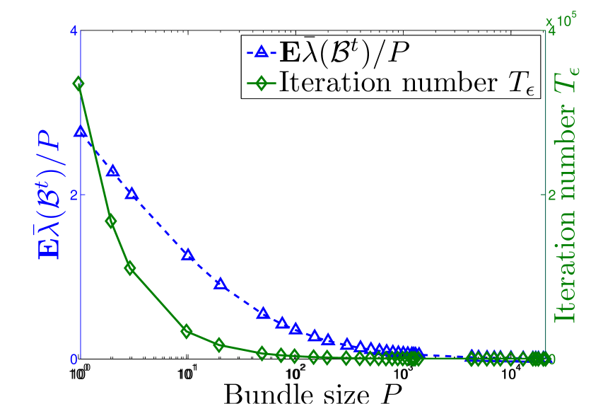
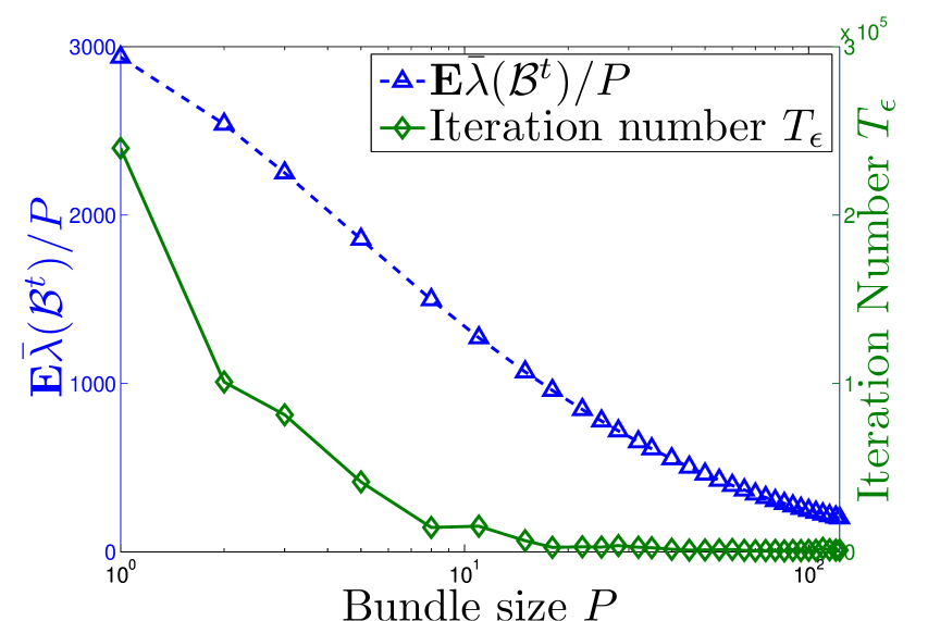
Figure 1: 𝐄​[λ¯​(ℬt)]/P𝐄delimited-[]Β―πœ†superscriptℬ𝑑𝑃\mathbf{E}[\bar{\lambda}(\mathcal{B}^{t})]/P and TΟ΅subscript𝑇italic-Ο΅T_{\epsilon} as a function of bundle size P𝑃P.

To verify the upper bound TΟ΅upsuperscriptsubscript𝑇italic-Ο΅upT_{\epsilon}^{\mathrm{up}} (17) of the iteration number TΟ΅subscript𝑇italic-Ο΅T_{\epsilon} for a given accuracy Ο΅italic-Ο΅\epsilon, we set Ο΅=10βˆ’3italic-Ο΅superscript103\epsilon=10^{-3} and show the iteration number TΟ΅subscript𝑇italic-Ο΅T_{\epsilon} as a function of the bundle size P𝑃P in FigureΒ 1, where two document datasets, a9a and real-sim (See SectionΒ 5.1 for details about the datasets) are used. Since TΟ΅upsuperscriptsubscript𝑇italic-Ο΅upT_{\epsilon}^{\mathrm{up}} is proportional to 𝐄​[λ¯​(ℬt)]/P𝐄delimited-[]Β―πœ†superscriptℬ𝑑𝑃{\mathbf{E}[\bar{\lambda}(\mathcal{B}^{t})]}/{P}, we plot 𝐄​[λ¯​(ℬt)]/P𝐄delimited-[]Β―πœ†superscriptℬ𝑑𝑃{\mathbf{E}[\bar{\lambda}(\mathcal{B}^{t})]}/{P} instead of TΟ΅upsuperscriptsubscript𝑇italic-Ο΅upT_{\epsilon}^{\mathrm{up}} in FigureΒ 1. The results match the upper bound inΒ (17): for given Ο΅italic-Ο΅\epsilon, TΟ΅subscript𝑇italic-Ο΅T_{\epsilon} (solid green lines) is positively correlated with 𝐄​[λ¯​(ℬt)]/P𝐄delimited-[]Β―πœ†superscriptℬ𝑑𝑃\mathbf{E}[\bar{\lambda}(\mathcal{B}^{t})]/P (dotted blue lines). In addition, TΟ΅subscript𝑇italic-Ο΅T_{\epsilon} decreases with respect to P𝑃P. These results show that with larger bundle size P𝑃P, fewer iterations are needed by the PCDN algorithm to converge to Ο΅italic-Ο΅\epsilon accuracy.

5 Experiments

In this section we present experimental results of the proposed PCDN algorithm, with comparisons to the state-of-the-art methods on L1subscript𝐿1L_{1}-regularized loss minimization problems using several benchmark datasets.

5.1 Experimental Setup

Table 2: Summary of datasets:. is The number of non-zero elements (NNZs) in training data is denoted by β€œtrain NNZ”; the average number of NNZs in the data corresponding to each feature is β€œNNZ/feature” denotes; ; β€œspa.” means train data sparsity, which is the ratio of zero elements in 𝐗𝐗\mathbf{X}; β€œcβˆ—superscript𝑐c^{*} SVM” and β€œcβˆ—superscript𝑐c^{*} logistic” denote the best regularization parameter cβˆ—superscript𝑐c^{*} for L2subscript𝐿2L_{2}-loss SVM and logistic regression, respectively, which are determined according to [24].
Dataset s𝑠s n𝑛n train NNZ NNZ/feature spa./% cβˆ—superscript𝑐c^{*} SVM cβˆ—superscript𝑐c^{*} logistic
a9a 26,049 123 361,278 2,937 88.72 0.5 2.0
real-sim 57,848 20,958 2,968,110 142 99.76 1.0 4.0
news20 15,997 1,355,191 7,281,110 5 99.97 64.0 64.0
gisette 6,000 5,000 29,729,997 5,946 0.9 0.25 0.25
rcv1 541,920 47,236 39,625,144 839 99.85 1.0 4.0
kdda 8,407,752 20,216,830 305,613,510 15 99.99 1.0 1.0
webspam 280,000 16,609,143 1,043,724,776 63 99.9775 64.0 64.0

Datasets.

Seven benchmark datasets444The datasets are available at http://www.csie.ntu.edu.tw/~cjlin/libsvmtools/datasets. are used in our experiments and the characteristics are summarized in Table 2. The news20, rcv1, a9a and real-sim datasets consist of document data points that are normalized to unit vectors. The a9a dataset is from UCI data repository, and the gisette set consists of handwriting digit data points from the NIPS 2003 feature selection challenge where features are linearly scaled to the [βˆ’1,1]11[-1,1] interval. The kdda dataset has been used for the KDD Cup 2010 data mining competition. The webspam dataset is the collection of Web pages that are created to manipulate search engines and deceive Web users.

Bundle Size Choice.

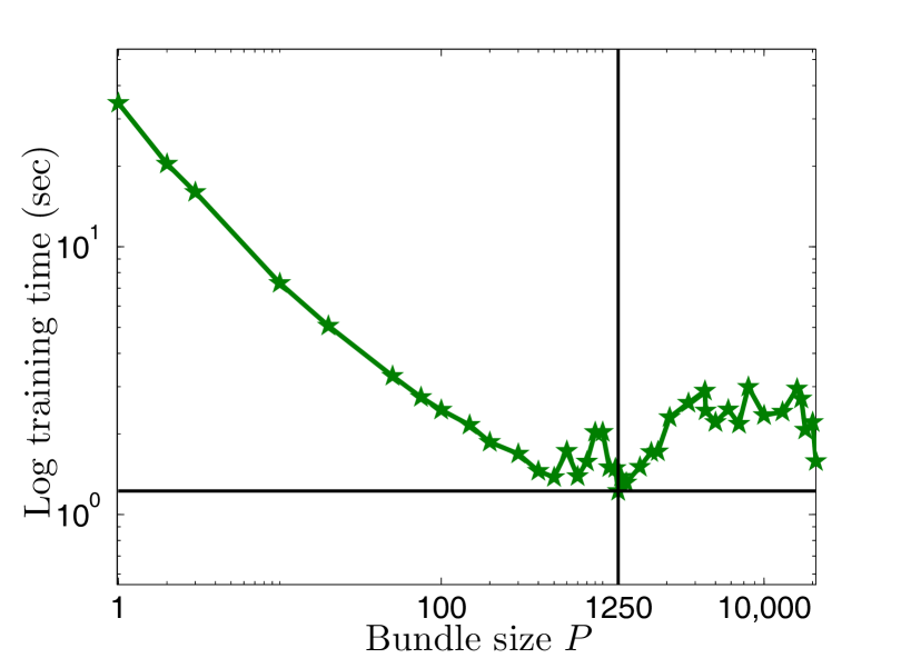
For each dataset, the optimal bundle size Pβˆ—superscript𝑃P^{*} under which the PCDN algorithm achieves minimum runtime is determined as follows. For AlgorithmΒ 3, the expected runtime of the t𝑑t-th inner iteration of PCDN time​(t)time𝑑\mathrm{time}(t) can be approximated by

𝐄​[time​(t)]β‰ˆ(P/#​thread)β‹…td​c+𝐄​[qt]β‹…tl​s,𝐄delimited-[]time𝑑⋅𝑃#threadsubscript𝑑𝑑𝑐⋅𝐄delimited-[]superscriptπ‘žπ‘‘subscript𝑑𝑙𝑠\mathbf{E}[\mathrm{time}(t)]\approx(P/\#\mathrm{thread})\cdot t_{dc}+\mathbf{E}[q^{t}]\cdot t_{ls}, (18)

where the expectation is based on a random choice of ℬtsuperscriptℬ𝑑\mathcal{B}^{t}; #​thread#thread\#\mathrm{thread} is the number of threads used by PCDN and fixed to be 23 in our experiments; td​csubscript𝑑𝑑𝑐t_{dc} is the time for computing the descent direction (stepΒ 3 in AlgorithmΒ 3); tl​ssubscript𝑑𝑙𝑠t_{ls} is the time for a step of P𝑃P-dimensional line search, which is approximately constant with varying P𝑃P (as shown in Section B of the appendix).
Refer to caption
(a) Logistic regression
Refer to caption
(b) L2subscript𝐿2L_{2}-loss SVM classification
Figure 2: Training time v.s. bundle size P𝑃P for the real-sim dataset with stopping criteria Ο΅=10βˆ’3italic-Ο΅superscript103\epsilon=10^{-3}, the intersection of the horizontal and vertical black line shows the optimal bundle size Pβˆ—superscript𝑃P^{*}.
Table 3: Optimal bundle size Pβˆ—superscript𝑃P^{*} for each dataset. #​thread=23#thread23\#\mathrm{thread}=23. The second row shows Pβˆ—superscript𝑃P^{*} for logistic regression, the third row shows Pβˆ—superscript𝑃P^{*} for L2subscript𝐿2L_{2}-loss SVM.
a9a real-sim news20 gisette rcv1 kdda webspam
123 1250 400 20 1600 29500 31750
85 500 150 15 350 95000 86000

As 𝐄​[qt]𝐄delimited-[]superscriptπ‘žπ‘‘\mathbf{E}[q^{t}] increases with respect to the bundle size P𝑃P (based on TheoremΒ 1), 𝐄​[time​(t)]𝐄delimited-[]time𝑑\mathbf{E}[\mathrm{time}(t)] increases with respect to P𝑃P based on (18). In addition, as the PCDN algorithm requires fewer iterations for larger P𝑃P to converge to Ο΅italic-Ο΅\epsilon accuracy (fromΒ (17) in SectionΒ 4), it is essential to make a trade-off between the increasing runtime per iteration 𝐄​[time​(t)]𝐄delimited-[]time𝑑\mathbf{E}[\mathrm{time}(t)] and the decreasing iteration number TΟ΅subscript𝑇italic-Ο΅T_{\epsilon} to select the optimal bundle size Pβˆ—superscript𝑃P^{*}. In practice, we run PCDN with varying P𝑃P. FigureΒ 2 shows the training time as a function of bundle size P𝑃P for the real-sim dataset and the optimal bundle size Pβˆ—superscript𝑃P^{*} can be determined. In this work, we empirically select the optimal Pβˆ—superscript𝑃P^{*} for each dataset (See TableΒ 3).

We note that it is not necessary to obtain the optimal P𝑃P to achieve significant speedup, as a wide range of P𝑃P will suffice to achieve the same goal in practice. As shown in FigureΒ 2(a), when P𝑃P is greater than 500, it achieves considerable speedup higher than SCDN (5 times faster than SCDN for P𝑃P=500). For a new dataset, one can first select a relatively large P𝑃P (about 5% of #features) with the most relaxed stopping criteria for a pilot experiment, and then adjust P𝑃P for best performance when necessary.

Evaluated Methods.

We evaluate the proposed PCDN algorithm against the state-of-the-art L1subscript𝐿1L_{1}-regularized optimization approaches, including newGLMNET [25], CDNΒ [24], Shotgun-CDN (SCDN)555Since the experimental validation in [2] has shown that SCDN is much faster than the SGD-type algorithms (including SGD, Parallel SGD [26; 16], and SMIDAS [21]) for datasets with more features, and SCDN performs well on datasets with more samples than features, we only compare the PCDN algorithm with the SCDN scheme here. The SCDN algorithm is also a competitive representative of the generic parallel coordinate descent algorithms in [19].Β [2], interior-point method (IPM) [8] and trust region Newton (TRON)Β [12] methods with C/C++ implementations. For the Armijo line search procedure (6) in the PCDN, CDN and SCDN methods, we set Οƒ=0.01𝜎0.01\sigma=0.01, Ξ³=0𝛾0\gamma=0 and Ξ²=0.5𝛽0.5\beta=0.5 for fair comparisons. The OpenMP library is used for parallel programming. The stopping criteria used in the experiments are similar to the outer stopping condition used inΒ [25].

The source code of the proposed PCDN algorithm will be made available to the public, and the implementation details are listed below:

  • β€’

    CDN: we implement this method based on the source code in the LIBLINEAR666liblinear version 1.7, http://www.csie.ntu.edu.tw/~cjlin/liblinear/. toolbox. Since the shrinking procedure cannot be performed inside the parallel loop of the SCDN and PCDN methods, we use an equivalent implementation of the CDN scheme for fair comparisons, where the shrinking procedure is modified such that it is consistent with the other parallel algorithms.

  • β€’

    SCDN: We set PΒ―=8¯𝑃8\bar{P}=8 for the SCDN method following Bradley et al.Β [2].

  • β€’

    PCDN: We implement this algorithm with conditions consistent with all other methods.

  • β€’

    TRON: We set Οƒ=0.01𝜎0.01\sigma=0.01 and Ξ²=0.1𝛽0.1\beta=0.1 in the projected line search according to Yuan et al.Β [24]. We use it as baseline algorithm for L2subscript𝐿2L_{2}-loss SVM.

  • β€’

    newGLMNET: We use the same setting and implementation provided by Yuan et al. [25]. Since it is outperformed by CDN for L2subscript𝐿2L_{2}-loss SVM, we only use it as baseline algorithm for logistic regression experiments.

  • β€’

    IPM: We use the source code777version 0.8.2, http://www.stanford.edu/~boyd/l1_logreg/ and default settings in [8]. We use it as a baseline interior-point algorithm for logistic regression.

Platform.

All experiments are carried out on a 64 bit machine with Intel Xeon 2.4 GHz CPU and 64 GB main memory. We set #​thread=23#thread23\#\mathrm{thread}=23 for PCDN on a 24-core machine, which is far less than the optimal bundle size Pβˆ—superscript𝑃P^{*} given in TableΒ 3. We note that the descent direction (stepΒ 3 in AlgorithmΒ 3) of the PCDN algorithm can be fully parallelized on several hundreds even to thousands of threads.

5.2 L1subscript𝐿1L_{1}-Regularized L2subscript𝐿2L_{2}-Loss SVM

Refer to caption Refer to caption Refer to caption
(a) rcv1 cβˆ—superscript𝑐c^{*} = 4.0 (b) news20 cβˆ—superscript𝑐c^{*} = 64.0 (c) a9a cβˆ—superscript𝑐c^{*} = 0.5
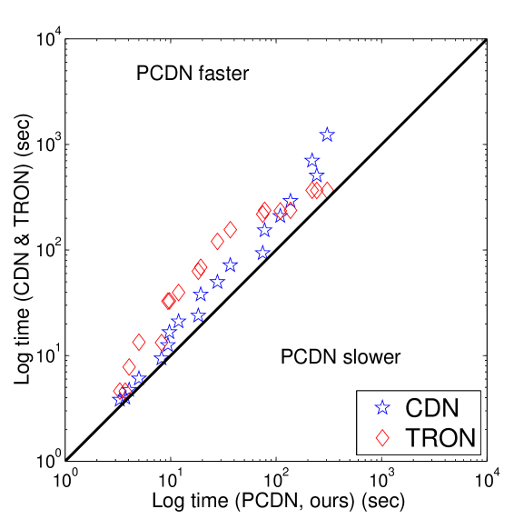
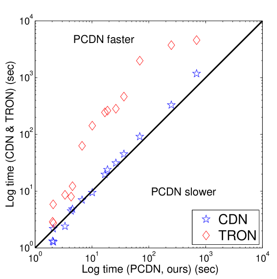
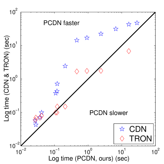
Figure 3: Runtime comparisons for L2subscript𝐿2L_{2}-loss SVM classification where each marker compares a solver with PCDN on one dataset. The y𝑦y-axis and xπ‘₯x-axis show the runtime of a solver as well as PCDN on the same problem. Markers above the diagonal line indicate that PCDN is faster.

FigureΒ 3 shows the runtime performance of the PCDN, CDN and TRON methods with the best regularization parameter cβˆ—superscript𝑐c^{*} (determined based on Yuan et al.Β [24]) and varying stopping criteria Ο΅italic-Ο΅\epsilon (equivalent for three solvers). Experimental results show that the proposed PCDN algorithm performs favorably against the other methods. As a feature-based parallel algorithm, the proposed PCDN solver performs well for sparse datasets with more features as shown by the results on the rcv1 and news20 datasets, which are very sparse (training data sparsity, defined by the ratio of zero elements in design matrix 𝐗𝐗\mathbf{X} and explained in Table 2, is 99.85%percent99.8599.85\% and 99.97%percent99.9799.97\%, respectively) with a large number of features (47,236 and 1,355,191). In such cases, the PCDN algorithm performs well against the TRON method. For the news20 dataset, the PCDN solver is 29 times faster than TRON method and 18 times faster than CDN approach. We note that for the a9a dataset, the PCDN solver is sometimes slightly slower than the TRON method since it is a relatively dense dataset with fewer features than samples (only 123 features with 26,049 samples).

5.3 L1subscript𝐿1L_{1}-Regularized Logistic Regression

(a) rcv1 Ο΅italic-Ο΅\epsilon = 10βˆ’3superscript10310^{-3} Refer to caption Refer to caption
(b) gisette Ο΅italic-Ο΅\epsilon = 10βˆ’4superscript10410^{-4} Refer to caption Refer to caption
(c) real-sim Ο΅italic-Ο΅\epsilon = 10βˆ’6superscript10610^{-6} Refer to caption Refer to caption
(d) kdda Ο΅italic-Ο΅\epsilon = 3.7βˆ—10βˆ’33.7superscript1033.7*10^{-3} Refer to caption Refer to caption
(e) webspam Ο΅italic-Ο΅\epsilon = 10βˆ’2superscript10210^{-2} Refer to caption Refer to caption
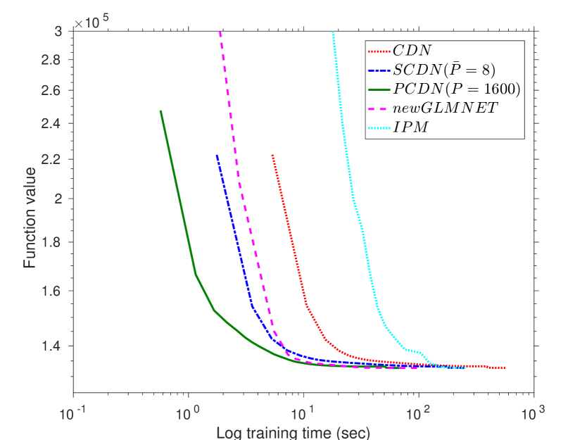
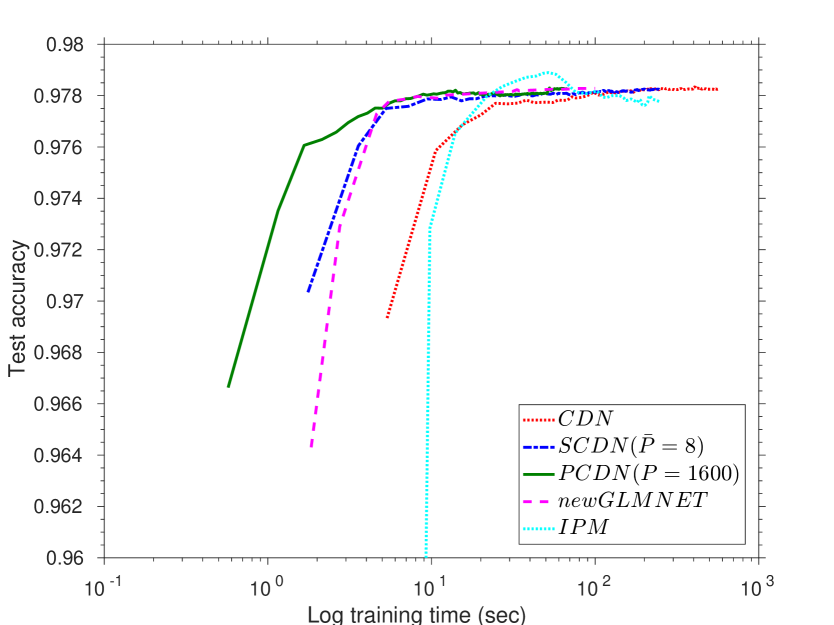
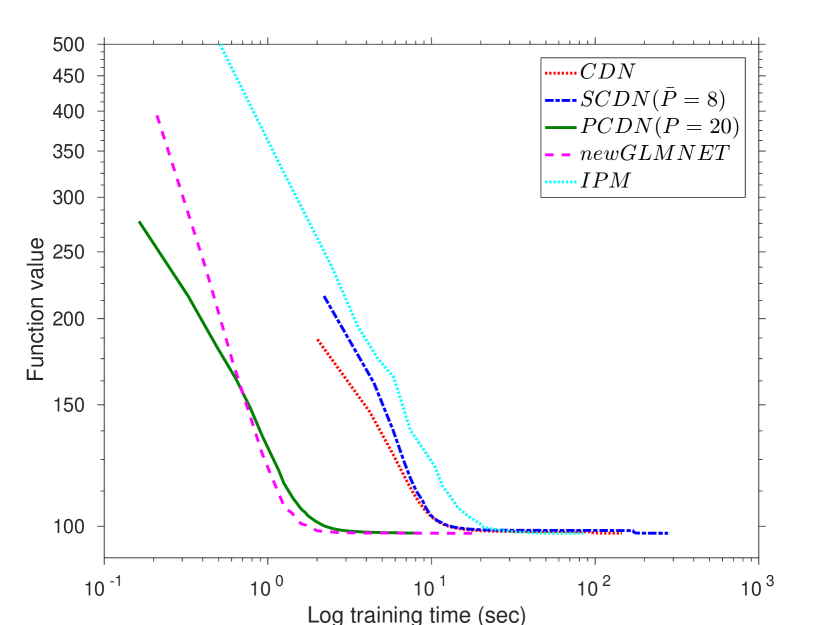
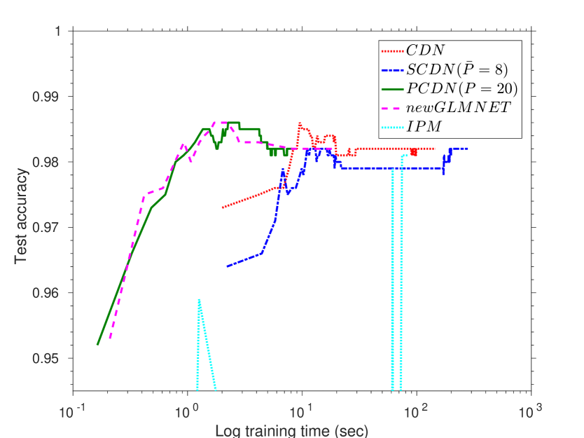
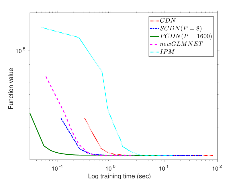
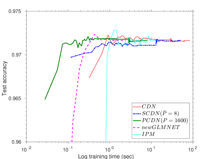
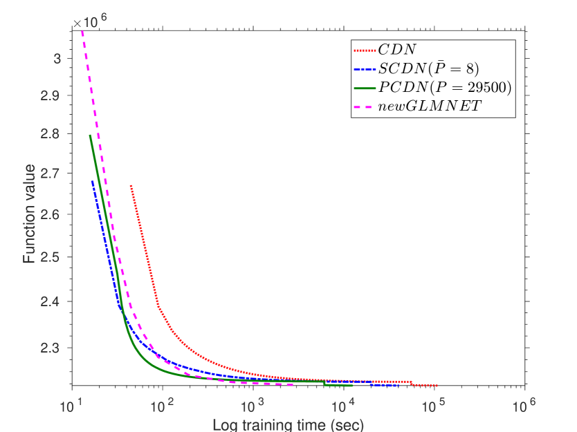
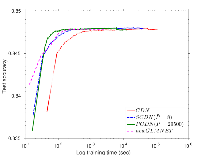
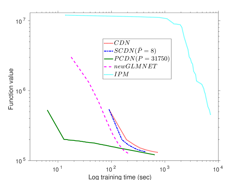
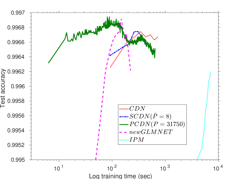
Figure 4: Runtime performance of PCDN, newGLMNET, SCDN, IPM and CDN for logistic regression. First column: function value. Second column: test accuracy.

We compare the runtime performance of the PCDN algorithm with the newGLMNET, IPM, SCDN and CDN methods on L1subscript𝐿1L_{1}-regularized logistic regression with a bias term. FigureΒ 4 shows the trace of function value (row 1) and test accuracy (row 2) with respect to the log runtime. Overall, the PCDN solver performs favorably against the other methods where the best speedup over the CDN method is 17.49 (with #​thread=23#thread23\#\mathrm{thread}=23). The speedup can be higher if more threads are used. For the rcv1 dataset in FigureΒ 4(a), the bundle size which reflects parallelism of PCDN is as high as 1,600.

For the gisette dataset shown in FigureΒ 4(b), the SCDN method is slower than the CDN scheme. This can be attributed to that the SCDN method is sensitive to correlation among features. Note that for gisette with 6,000 features the optimal Pβˆ—superscript𝑃P^{*} for PCDN is only 20, which also indicates the high correlation among features. For the kdda dataset, the computational load for IPM is prohibitively long, and not included in FigureΒ 4(d). Despite the required runtime, the IPM method achieves higher accuracy on the rcv1 and real-sim datasets.

FigureΒ 4(e) shows that the PCDN performs favorably against the state-of-the-art methods on the large webspam dataset which consists of 1,043,724,776 non-zero elements. For the kdda dataset, the PCDN algorithm is slower than the SCDN method in the beginning but converges faster than the others in the end as shown in Figure 4(d). Except for the correlation among features and memory bandwidth limit, another issue that would significantly affect the performance of PCDN is the workload of the parallel threads. For the PCDN algorithm, each thread first processes one feature of the data, and then switches to the next feature. Thus, the parallel processing time of PCDN, which contributes to the acceleration, is proportional to the workload of the parallel threads. The workload of each thread is approximately proportional to the number of non-zero elements (NNZs) of the data corresponding to the feature being processed. To verify that, we compute the average number of NNZs per feature (NNZ/feature column in Table 2), and show that there are only 15 NNZs/feature in the kdda dataset, while there are 63 NNZs/feature in the webspam dataset. These results explain the performance difference of the PCDN algorithm on these two large datasets.

5.4 Scalability of PCDN

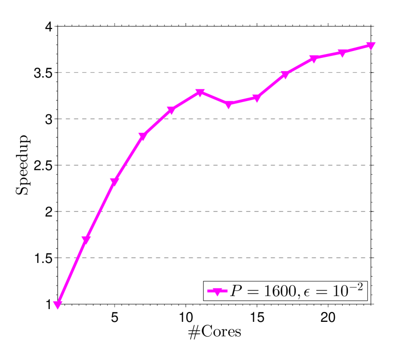
We also evaluate the scalability of PCDN in two aspects: whether PCDN can maintain the speed-up when the data size is increased, and whether PCDN can achieve better speed-up when the available computing resource (e.g., number of cores) is increased.

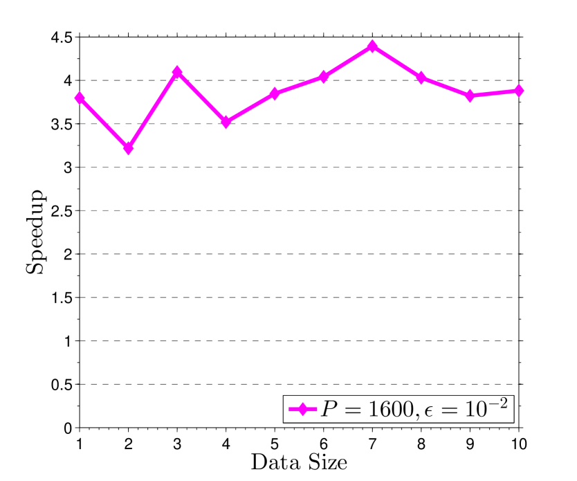
To analyze the effect of data size, we maintain all the other factors, e.g., correlation among features, the same in the experiments. To this end, we duplicate the samples to create datasets from 100% of original size to 2000%. Figure 5 shows the scalability over different number of cores and data size.
Refer to caption Refer to caption
(a) different #core (b) different data size
Figure 5: Speedup of PCDN on the rcv1 dataset.

Effect of Number of Cores.

Figure 5(a) shows that the speedup of the PCDN algorithm is larger at the beginning when the number of cores is increased (i.e., the parallel efficiency decreases with more parallelism) which can be explained by the Amdahl’s law: First, as the number of cores increase, the parallelized part takes less and less time. However, the serial part takes approximately the same constant time. Second, with more cores, there is increasing parallelization overhead, e.g., more data transfer, and thereby lowering parallel efficiency.

Effect of Data Size.

Figure 5(b) shows that the speedup is approximately constant with larger data size, which shows the weak scaling property of parallel algorithms. It is noteworthy that for very large dataset, the size of the data for each feature is also quite large that it may exceed the memory bandwidth.

5.5 Discussions

The high dimensional line search plays the key role in ensuring global convergence of PCDN. In this work, we use the Armijo line search as a specific realization, and it is worth exploring other ways to perform the line search. In addition, the computational cost of line search can be further reduced by deriving the (approximate) optimal line search step number, as what is performed for solving the dual linear SVM problem in [10].

The bundle size P𝑃P controls the ratio between computation and communication, and thus affecting the running time of PCDN. Although we present an empirical method to choose a good P𝑃P in Section 5.1, it is of great interest to develop a principled approach to determine the optimal value for P𝑃P.

Another direction to pursue is to extend the PCDN algorithm within a distributed framework in a way similar to the Parallel SGDΒ [27] and Downpour SGDΒ [5] methods, to deal with very large datasets with lots of samples, that do not fit into one single machine. This can be achieved by first randomly distributing training data of different samples to different machines (i.e., parallelizing over samples), and applying the PCDN algorithm over a subset (i.e., parallelizing over features) on each machine, and aggregating all the models in the end. As a shared memory parallel algorithm, the PCDN algorithm can also be implemented with the stale synchronous parallel modelΒ [7] to achieve better performance.

6 Concluding Remarks

We propose an algorithm termed Parallel Coordinate Descent with approximate Newton step, with strong convergence guarantee, fast convergence rate and high parallelism for L1subscript𝐿1L_{1}-regularized minimization problems. We show that the seemingly expensive high dimensional line search can be calculated efficiently with the implementation technique of maintaining intermediate quantities, which also minimizes the data transfer and synchronization cost of PCDN.

The PCDN can be generalized to solve the problems of minimizing the sum of a convex twice differentiable loss term and a separable regularization term. Thus, it allows L1subscript𝐿1L_{1} (lasso), L2subscript𝐿2L_{2} (ridge regression), and mixtures of the two penalties (elastic net). Experimental results on several benchmark datasets show that the proposed PCDN algorithm performs favorably against several state-of-the-art methods for L1subscript𝐿1L_{1}-regularized optimization problems.

Acknowledgments

The authors would like to thank Hongyuan Zha, Xiangfeng Wang, Martin TakΓ‘c and Martin Jaggi for their valuable comments and suggestions to improve this work. This research was partially supported by the Max Planck ETH Center for Learning Systems

References

  • Bian etΒ al. [2013] Yatao Bian, Xiong Li, Mingqi Cao, and Yuncai Liu. Bundle cdn: A highly parallelized approach for large-scale l1-regularized logistic regression. In ECML/PKDD, pages 81–95, 2013.
  • Bradley etΒ al. [2011] JosephΒ K. Bradley, Aapo Kyrola, Danny Bickson, and Carlos Guestrin. Parallel coordinate descent for l1-regularized loss minimization. In ICML, pages 321–328, 2011.
  • Burke [1985] JamesV. Burke. Descent methods for composite nondifferentiable optimization problems. Mathematical Programming, 33(3):260–279, 1985.
  • Chang etΒ al. [2008] Kai-Wei Chang, Cho-Jui Hsieh, and Chih-Jen Lin. Coordinate descent method for large-scale l2-loss linear support vector machines. Journal of Machine Learning Research, 9:1369–1398, 2008.
  • Dean etΒ al. [2012] Jeffrey Dean, GregΒ S. Corrado, Rajat Monga, Kai Chen, Matthieu Devin, QuocΒ V. Le, MarkΒ Z. Mao, MarcΒ A. Ranzato, Andrew Senior, Paul Tucker, KeΒ Yang, and AndrewΒ Y. Ng. Large Scale Distributed Deep Networks. In NIPS, 2012.
  • Fan etΒ al. [2008] Rong-En Fan, Kai-Wei Chang, Cho-Jui Hsieh, Xiang-Rui Wang, and Chih-Jen Lin. Liblinear: A library for large linear classification. Journal of Machine Learning Research, 9:1871–1874, 2008.
  • Ho etΒ al. [2013] Q.Β Ho, J.Β Cipar, H.Β Cui, J.-K. Kim, S.Β Lee, P.Β B. Gibbons, G.Β Gibson, G.Β R. Ganger, and E.Β P. Xing. More effective distributed ml via a stale synchronous parallel parameter server. In NIPS, 2013.
  • Koh etΒ al. [2007] Kwangmoo Koh, Seung-Jean Kim, and StephenΒ P Boyd. An interior-point method for large-scale l1-regularized logistic regression. Journal of Machine learning research, 8(8):1519–1555, 2007.
  • Langford etΒ al. [2009] John Langford, Lihong Li, and Tong Zhang. Sparse online learning via truncated gradient. Journal of Machine Learning Research, 10:777–801, 2009.
  • Lee and Roth [2015] Ching-Pei Lee and Dan Roth. Distributed box-constrained quadratic optimization for dual linear SVM. In ICML, Lille, France, 2015, pages 987–996, 2015. URL http://jmlr.org/proceedings/papers/v37/leea15.html.
  • Lee etΒ al. [2009] Honglak Lee, Roger Grosse, Rajesh Ranganath, and AndrewΒ Y. Ng. Convolutional deep belief networks for scalable unsupervised learning of hierarchical representations. In ICML, pages 609–616, 2009.
  • Lin and MorΓ© [1999] Chih-Jen Lin and JorgeΒ J. MorΓ©. Newton’s method for large bound-constrained optimization problems. SIAM Journal on Optimization, 9(4):1100–1127, 1999.
  • Luo etΒ al. [2014] Haipeng Luo, Patrick Haffner, and Jean-FranΓ§ois Paiement. Accelerated parallel optimization methods for large scale machine learning. arXiv:1411.6725, 2014.
  • Marecek etΒ al. [2014] Jakub Marecek, Peter RichtΓ‘rik, and Martin TakΓ‘c. Distributed block coordinate descent for minimizing partially separable functions. arXiv:1406.0238, 2014.
  • Ng [2004] AndrewΒ Y. Ng. Feature selection, l1 vs. l2 regularization, and rotational invariance. In ICML, pages 78–85, 2004.
  • Niu etΒ al. [2011] Feng Niu, Benjamin Recht, Christopher Re, and StephenΒ J. Wright. Hogwild: A lock-free approach to parallelizing stochastic gradient descent. In NIPS, pages 693–701, 2011.
  • RichtΓ‘rik and TakΓ‘c [2012] Peter RichtΓ‘rik and Martin TakΓ‘c. Parallel coordinate descent methods for big data optimization. CoRR, abs/1212.0873, 2012.
  • RichtΓ‘rik and TakÑč [2013] Peter RichtΓ‘rik and Martin TakÑč. Distributed coordinate descent method for learning with big data. arXiv:1310.2059, 2013.
  • Scherrer etΒ al. [2012a] Chad Scherrer, Mahantesh Halappanavar, Ambuj Tewari, and David Haglin. Scaling up coordinate descent algorithms for large l1-regularization problems. In ICML, 2012a. URL http://icml.cc/discuss/2012/705.html.
  • Scherrer etΒ al. [2012b] Chad Scherrer, Ambuj Tewari, Mahantesh Halappanavar, and David Haglin. Feature clustering for accelerating parallel coordinate descent. In NIPS, pages 28–36, 2012b.
  • Shalev-Shwartz and Tewari [2009] Shai Shalev-Shwartz and Ambuj Tewari. Stochastic methods for l11{}_{\mbox{1}} regularized loss minimization. In ICML, pages 117–124, 2009.
  • Tseng and Yun [2009] Paul Tseng and Sangwoon Yun. A coordinate gradient descent method for nonsmooth separable minimization. Mathematical Programming, 117(1-2):387–423, 2009.
  • Wright etΒ al. [2009] John Wright, AllenΒ Y. Yang, Arvind Ganesh, ShankarΒ S. Sastry, and YiΒ Ma. Robust face recognition via sparse representation. IEEE Transactions on Pattern Analysis and Machine Intelligence, 31(2):210–227, 2009.
  • Yuan etΒ al. [2010] Guo-Xun Yuan, Kai-Wei Chang, Cho-Jui Hsieh, and Chih-Jen Lin. A comparison of optimization methods and software for large-scale l1-regularized linear classification. Journal of Machine Learning Research, 11:3183–3234, 2010.
  • Yuan etΒ al. [2011] Guo-Xun Yuan, Chia-Hua Ho, and Chih-Jen Lin. An improved glmnet for l1-regularized logistic regression. In KDD, pages 33–41, 2011.
  • Zinkevich etΒ al. [2009] Martin Zinkevich, Alex Smola, and John Langford. Slow learners are fast. In NIPS, pages 2331–2339, 2009.
  • Zinkevich etΒ al. [2010] Martin Zinkevich, Markus Weimer, AlexanderΒ J. Smola, and Lihong Li. Parallelized stochastic gradient descent. In NIPS, pages 2595–2603, 2010.

Appendix

Appendix A Full Proofs of Theorems 1 and 2

A.1 Proof of Lemma 1(a)

Proof.

(1)   We first prove that 𝐄ℬt​[λ¯​(ℬt)]subscript𝐄superscriptℬ𝑑delimited-[]Β―πœ†superscriptℬ𝑑\mathbf{E}_{\mathcal{B}^{t}}[\bar{\lambda}(\mathcal{B}^{t})] is monotonically increasing with respect to P𝑃P and 𝐄ℬt​[λ¯​(ℬt)]subscript𝐄superscriptℬ𝑑delimited-[]Β―πœ†superscriptℬ𝑑\mathbf{E}_{\mathcal{B}^{t}}[\bar{\lambda}(\mathcal{B}^{t})] is constant with respect to P𝑃P, if Ξ»isubscriptπœ†π‘–\lambda_{i} is constant or Ξ»1=Ξ»2=β‹―=Ξ»nsubscriptπœ†1subscriptπœ†2β‹―subscriptπœ†π‘›\lambda_{1}=\lambda_{2}=\cdots=\lambda_{n}.

Let Ξ»ksubscriptπœ†π‘˜\lambda_{k} be the kπ‘˜k-th minimum of (π—βŠ€β€‹π—)j​j,j=1,β‹―,nformulae-sequencesubscriptsuperscript𝐗top𝐗𝑗𝑗𝑗1⋯𝑛(\mathbf{X}^{\top}\mathbf{X})_{jj},j=1,\cdots,n, for 1≀P≀n1𝑃𝑛1\leq P\leq n. We define

f​(P):=𝐄ℬt​[λ¯​(ℬt)]=(Ξ»n​Cnβˆ’1Pβˆ’1+β‹―+Ξ»k​Ckβˆ’1Pβˆ’1+β‹―+Ξ»P​CPβˆ’1Pβˆ’1)/CnP,assign𝑓𝑃subscript𝐄superscriptℬ𝑑delimited-[]Β―πœ†superscriptℬ𝑑subscriptπœ†π‘›superscriptsubscript𝐢𝑛1𝑃1β‹―subscriptπœ†π‘˜superscriptsubscriptπΆπ‘˜1𝑃1β‹―subscriptπœ†π‘ƒsuperscriptsubscript𝐢𝑃1𝑃1superscriptsubscript𝐢𝑛𝑃\begin{split}&f(P):=\mathbf{E}_{\mathcal{B}^{t}}[\bar{\lambda}(\mathcal{B}^{t})]=\\ &(\lambda_{n}C_{n-1}^{P-1}+\cdots+\lambda_{k}C_{k-1}^{P-1}+\cdots+\lambda_{P}C_{P-1}^{P-1})/C_{n}^{P},\end{split} (19)

where CnPsuperscriptsubscript𝐢𝑛𝑃C_{n}^{P} is a binomial coefficient. For 1≀P≀nβˆ’11𝑃𝑛11\leq P\leq n-1,

f​(P+1)βˆ’f​(P)𝑓𝑃1𝑓𝑃\displaystyle f(P+1)-f(P)
=βˆ’Ξ»P​CPβˆ’1Pβˆ’1CnP+βˆ‘k=nP+1Ξ»k​(Ckβˆ’1PCnP+1βˆ’Ckβˆ’1Pβˆ’1CnP)absentsubscriptπœ†π‘ƒsuperscriptsubscript𝐢𝑃1𝑃1superscriptsubscript𝐢𝑛𝑃superscriptsubscriptπ‘˜π‘›π‘ƒ1subscriptπœ†π‘˜superscriptsubscriptπΆπ‘˜1𝑃superscriptsubscript𝐢𝑛𝑃1superscriptsubscriptπΆπ‘˜1𝑃1superscriptsubscript𝐢𝑛𝑃\displaystyle=-\lambda_{P}\frac{C_{P-1}^{P-1}}{C_{n}^{P}}+\sum_{k=n}^{P+1}\lambda_{k}(\frac{C_{k-1}^{P}}{C_{n}^{P+1}}-\frac{C_{k-1}^{P-1}}{C_{n}^{P}})
=βˆ’Ξ»P​CPβˆ’1Pβˆ’1CnP+βˆ‘k=nP+1Ξ»k​(P+1)​kβˆ’P​(n+1)P​(nβˆ’P)​Ckβˆ’1Pβˆ’1CnP.absentsubscriptπœ†π‘ƒsuperscriptsubscript𝐢𝑃1𝑃1superscriptsubscript𝐢𝑛𝑃superscriptsubscriptπ‘˜π‘›π‘ƒ1subscriptπœ†π‘˜π‘ƒ1π‘˜π‘ƒπ‘›1𝑃𝑛𝑃superscriptsubscriptπΆπ‘˜1𝑃1superscriptsubscript𝐢𝑛𝑃\displaystyle=-\lambda_{P}\frac{C_{P-1}^{P-1}}{C_{n}^{P}}+\sum_{k=n}^{P+1}\lambda_{k}\frac{(P+1)k-P(n+1)}{P(n-P)}\frac{C_{k-1}^{P-1}}{C_{n}^{P}}.

When kΒ―=⌈(P+1)​kP​(n+1)βŒ‰Β―π‘˜π‘ƒ1π‘˜π‘ƒπ‘›1\bar{k}=\lceil\frac{(P+1)k}{P(n+1)}\rceil, then (P+1)​kβˆ’P​(n+1)β‰₯0,βˆ€kβ‰₯kΒ―formulae-sequence𝑃1π‘˜π‘ƒπ‘›10for-allπ‘˜Β―π‘˜(P+1)k-P(n+1)\geq 0,\forall k\geq\bar{k}, and (P+1)​kβˆ’P​(n+1)≀0,βˆ€k<kΒ―formulae-sequence𝑃1π‘˜π‘ƒπ‘›10for-allπ‘˜Β―π‘˜(P+1)k-P(n+1)\leq 0,\forall k<\bar{k}. The above equation is equivalent to

f​(P+1)βˆ’f​(P)=𝑓𝑃1𝑓𝑃absent\displaystyle f(P+1)-f(P)=
[βˆ‘k=nkΒ―Ξ»k​(P+1)​kβˆ’P​(n+1)P​(nβˆ’P)​Ckβˆ’1Pβˆ’1CnP]βˆ’limit-fromdelimited-[]superscriptsubscriptπ‘˜π‘›Β―π‘˜subscriptπœ†π‘˜π‘ƒ1π‘˜π‘ƒπ‘›1𝑃𝑛𝑃superscriptsubscriptπΆπ‘˜1𝑃1superscriptsubscript𝐢𝑛𝑃\displaystyle\left[\sum_{k=n}^{\bar{k}}\lambda_{k}\frac{(P+1)k-P(n+1)}{P(n-P)}\frac{C_{k-1}^{P-1}}{C_{n}^{P}}\right]-
[βˆ‘k=kΒ―P+1Ξ»k​P​(n+1)βˆ’(P+1)​kP​(nβˆ’P)​Ckβˆ’1Pβˆ’1CnP]βˆ’Ξ»P​CPβˆ’1Pβˆ’1CnP.delimited-[]superscriptsubscriptπ‘˜Β―π‘˜π‘ƒ1subscriptπœ†π‘˜π‘ƒπ‘›1𝑃1π‘˜π‘ƒπ‘›π‘ƒsuperscriptsubscriptπΆπ‘˜1𝑃1superscriptsubscript𝐢𝑛𝑃subscriptπœ†π‘ƒsuperscriptsubscript𝐢𝑃1𝑃1superscriptsubscript𝐢𝑛𝑃\displaystyle\left[\sum_{k=\bar{k}}^{P+1}\lambda_{k}\frac{P(n+1)-(P+1)k}{P(n-P)}\frac{C_{k-1}^{P-1}}{C_{n}^{P}}\right]-\lambda_{P}\frac{C_{P-1}^{P-1}}{C_{n}^{P}}.

According to the observations that Ξ»kβ‰₯Ξ»kΒ―,βˆ€kβ‰₯kΒ―formulae-sequencesubscriptπœ†π‘˜subscriptπœ†Β―π‘˜for-allπ‘˜Β―π‘˜\lambda_{k}\geq\lambda_{\bar{k}},\forall k\geq\bar{k} and Ξ»k≀λkΒ―,βˆ€k<kΒ―formulae-sequencesubscriptπœ†π‘˜subscriptπœ†Β―π‘˜for-allπ‘˜Β―π‘˜\lambda_{k}\leq\lambda_{\bar{k}},\forall k<\bar{k}, we can decrease the above equation by substitute Ξ»ksubscriptπœ†π‘˜\lambda_{k} by Ξ»kΒ―subscriptπœ†Β―π‘˜\lambda_{\bar{k}}. That is,

f​(P+1)βˆ’f​(P)𝑓𝑃1𝑓𝑃\displaystyle f(P+1)-f(P)
β‰₯[βˆ‘k=nkΒ―Ξ»k¯​(P+1)​kβˆ’P​(n+1)P​(nβˆ’P)​Ckβˆ’1Pβˆ’1CnP]βˆ’absentlimit-fromdelimited-[]superscriptsubscriptπ‘˜π‘›Β―π‘˜subscriptπœ†Β―π‘˜π‘ƒ1π‘˜π‘ƒπ‘›1𝑃𝑛𝑃superscriptsubscriptπΆπ‘˜1𝑃1superscriptsubscript𝐢𝑛𝑃\displaystyle\geq\left[\sum_{k=n}^{\bar{k}}\lambda_{\bar{k}}\frac{(P+1)k-P(n+1)}{P(n-P)}\frac{C_{k-1}^{P-1}}{C_{n}^{P}}\right]-
[βˆ‘k=kΒ―P+1Ξ»k¯​P​(n+1)βˆ’(P+1)​kP​(nβˆ’P)​Ckβˆ’1Pβˆ’1CnP]βˆ’Ξ»k¯​CPβˆ’1Pβˆ’1CnPdelimited-[]superscriptsubscriptπ‘˜Β―π‘˜π‘ƒ1subscriptπœ†Β―π‘˜π‘ƒπ‘›1𝑃1π‘˜π‘ƒπ‘›π‘ƒsuperscriptsubscriptπΆπ‘˜1𝑃1superscriptsubscript𝐢𝑛𝑃subscriptπœ†Β―π‘˜superscriptsubscript𝐢𝑃1𝑃1superscriptsubscript𝐢𝑛𝑃\displaystyle\left[\sum_{k=\bar{k}}^{P+1}\lambda_{\bar{k}}\frac{P(n+1)-(P+1)k}{P(n-P)}\frac{C_{k-1}^{P-1}}{C_{n}^{P}}\right]-\lambda_{\bar{k}}\frac{C_{P-1}^{P-1}}{C_{n}^{P}}
=Ξ»k¯​[βˆ’CPβˆ’1Pβˆ’1CnP+βˆ‘k=nP+1(P+1)​kβˆ’P​(n+1)P​(nβˆ’P)​Ckβˆ’1Pβˆ’1CnP]absentsubscriptπœ†Β―π‘˜delimited-[]superscriptsubscript𝐢𝑃1𝑃1superscriptsubscript𝐢𝑛𝑃superscriptsubscriptπ‘˜π‘›π‘ƒ1𝑃1π‘˜π‘ƒπ‘›1𝑃𝑛𝑃superscriptsubscriptπΆπ‘˜1𝑃1superscriptsubscript𝐢𝑛𝑃\displaystyle=\lambda_{\bar{k}}\left[-\frac{C_{P-1}^{P-1}}{C_{n}^{P}}+\sum_{k=n}^{P+1}\frac{(P+1)k-P(n+1)}{P(n-P)}\frac{C_{k-1}^{P-1}}{C_{n}^{P}}\right]
=Ξ»k¯​[βˆ’CPβˆ’1Pβˆ’1CnP+βˆ‘k=nP+1(Ckβˆ’1PCnP+1βˆ’Ckβˆ’1Pβˆ’1CnP)]absentsubscriptπœ†Β―π‘˜delimited-[]superscriptsubscript𝐢𝑃1𝑃1superscriptsubscript𝐢𝑛𝑃superscriptsubscriptπ‘˜π‘›π‘ƒ1superscriptsubscriptπΆπ‘˜1𝑃superscriptsubscript𝐢𝑛𝑃1superscriptsubscriptπΆπ‘˜1𝑃1superscriptsubscript𝐢𝑛𝑃\displaystyle=\lambda_{\bar{k}}\left[-\frac{C_{P-1}^{P-1}}{C_{n}^{P}}+\sum_{k=n}^{P+1}(\frac{C_{k-1}^{P}}{C_{n}^{P+1}}-\frac{C_{k-1}^{P-1}}{C_{n}^{P}})\right]
=Ξ»k¯​[βˆ‘k=nP+1Ckβˆ’1PCnP+1βˆ’βˆ‘k=nPCkβˆ’1Pβˆ’1CnP]absentsubscriptπœ†Β―π‘˜delimited-[]superscriptsubscriptπ‘˜π‘›π‘ƒ1superscriptsubscriptπΆπ‘˜1𝑃superscriptsubscript𝐢𝑛𝑃1superscriptsubscriptπ‘˜π‘›π‘ƒsuperscriptsubscriptπΆπ‘˜1𝑃1superscriptsubscript𝐢𝑛𝑃\displaystyle=\lambda_{\bar{k}}\left[\sum_{k=n}^{P+1}\frac{C_{k-1}^{P}}{C_{n}^{P+1}}-\sum_{k=n}^{P}\frac{C_{k-1}^{P-1}}{C_{n}^{P}}\right]
=Ξ»k¯​[1βˆ’1]=0absentsubscriptπœ†Β―π‘˜delimited-[]110\displaystyle=\lambda_{\bar{k}}[1-1]=0

Thus, f​(P+1)βˆ’f​(P)β‰₯0,βˆ€1≀P≀nβˆ’1formulae-sequence𝑓𝑃1𝑓𝑃0for-all1𝑃𝑛1f(P+1)-f(P)\geq 0,\forall 1\leq P\leq n-1. Namely, 𝐄ℬt​λ¯​(ℬt)subscript𝐄superscriptβ„¬π‘‘Β―πœ†superscriptℬ𝑑\mathbf{E}_{\mathcal{B}^{t}}\bar{\lambda}(\mathcal{B}^{t}) is monotonically increasing with respect to P𝑃P. Clearly, fromΒ (19), if Ξ»1=Ξ»2=β‹―=Ξ»nsubscriptπœ†1subscriptπœ†2β‹―subscriptπœ†π‘›\lambda_{1}=\lambda_{2}=\cdots=\lambda_{n}, then 𝐄ℬt​[λ¯​(ℬt)]=Ξ»1subscript𝐄superscriptℬ𝑑delimited-[]Β―πœ†superscriptℬ𝑑subscriptπœ†1\mathbf{E}_{\mathcal{B}^{t}}[\bar{\lambda}(\mathcal{B}^{t})]=\lambda_{1}, which is constant with respect to P𝑃P.

(2) Next, we prove that 𝐄ℬt​[λ¯​(ℬt)]/Psubscript𝐄superscriptℬ𝑑delimited-[]Β―πœ†superscriptℬ𝑑𝑃{\mathbf{E}_{\mathcal{B}^{t}}[\bar{\lambda}(\mathcal{B}^{t})]}/{P} is monotonically decreasing with respect to P𝑃P. Let Ξ»ksubscriptπœ†π‘˜\lambda_{k} be the kπ‘˜k-th minimum of (π—βŠ€β€‹π—)j​j,j=1,β‹―,nformulae-sequencesubscriptsuperscript𝐗top𝐗𝑗𝑗𝑗1⋯𝑛(\mathbf{X}^{\top}\mathbf{X})_{jj},j=1,\cdots,n. For 1≀P≀n1𝑃𝑛1\leq P\leq n, define

g​(P):=𝐄ℬt​[λ¯​(ℬt)]P=1P​CnP​(Ξ»n​Cnβˆ’1Pβˆ’1+β‹―+Ξ»k​Ckβˆ’1Pβˆ’1+β‹―+Ξ»P​CPβˆ’1Pβˆ’1).assign𝑔𝑃subscript𝐄superscriptℬ𝑑delimited-[]Β―πœ†superscriptℬ𝑑𝑃1𝑃superscriptsubscript𝐢𝑛𝑃subscriptπœ†π‘›superscriptsubscript𝐢𝑛1𝑃1β‹―subscriptπœ†π‘˜superscriptsubscriptπΆπ‘˜1𝑃1β‹―subscriptπœ†π‘ƒsuperscriptsubscript𝐢𝑃1𝑃1\begin{split}&g(P):=\frac{\mathbf{E}_{\mathcal{B}^{t}}[\bar{\lambda}(\mathcal{B}^{t})]}{P}=\\ &\frac{1}{PC_{n}^{P}}(\lambda_{n}C_{n-1}^{P-1}+\cdots+\lambda_{k}C_{k-1}^{P-1}+\cdots+\lambda_{P}C_{P-1}^{P-1}).\end{split}

For 1≀P≀nβˆ’11𝑃𝑛11\leq P\leq n-1, we have

g​(P+1)βˆ’g​(P)𝑔𝑃1𝑔𝑃\displaystyle g(P+1)-g(P)
=βˆ’Ξ»P​CPβˆ’1Pβˆ’1P​CnP+βˆ‘k=nP+1Ξ»k​(Ckβˆ’1P(P+1)​CnP+1βˆ’Ckβˆ’1Pβˆ’1P​CnP)absentsubscriptπœ†π‘ƒsuperscriptsubscript𝐢𝑃1𝑃1𝑃superscriptsubscript𝐢𝑛𝑃superscriptsubscriptπ‘˜π‘›π‘ƒ1subscriptπœ†π‘˜superscriptsubscriptπΆπ‘˜1𝑃𝑃1superscriptsubscript𝐢𝑛𝑃1superscriptsubscriptπΆπ‘˜1𝑃1𝑃superscriptsubscript𝐢𝑛𝑃\displaystyle=-\lambda_{P}\frac{C_{P-1}^{P-1}}{PC_{n}^{P}}+\sum_{k=n}^{P+1}\lambda_{k}(\frac{C_{k-1}^{P}}{(P+1)C_{n}^{P+1}}-\frac{C_{k-1}^{P-1}}{PC_{n}^{P}})
=βˆ’Ξ»P​CPβˆ’1Pβˆ’1P​CnP+βˆ‘k=nP+1Ξ»k​kβˆ’nnβˆ’P​Ckβˆ’1Pβˆ’1P​CnP.absentsubscriptπœ†π‘ƒsuperscriptsubscript𝐢𝑃1𝑃1𝑃superscriptsubscript𝐢𝑛𝑃superscriptsubscriptπ‘˜π‘›π‘ƒ1subscriptπœ†π‘˜π‘˜π‘›π‘›π‘ƒsuperscriptsubscriptπΆπ‘˜1𝑃1𝑃superscriptsubscript𝐢𝑛𝑃\displaystyle=-\lambda_{P}\frac{C_{P-1}^{P-1}}{PC_{n}^{P}}+\sum_{k=n}^{P+1}\lambda_{k}\frac{k-n}{n-P}\frac{C_{k-1}^{P-1}}{PC_{n}^{P}}.

According to the observations that kβˆ’nnβˆ’P≀0π‘˜π‘›π‘›π‘ƒ0\frac{k-n}{n-P}\leq 0 and Ξ»kβ‰₯Ξ»P,βˆ€k=n,β‹―,P+1formulae-sequencesubscriptπœ†π‘˜subscriptπœ†π‘ƒfor-allπ‘˜π‘›β‹―π‘ƒ1\lambda_{k}\geq\lambda_{P},\forall k=n,\cdots,P+1, we can increase the above equation by substituting Ξ»ksubscriptπœ†π‘˜\lambda_{k} with Ξ»Psubscriptπœ†π‘ƒ\lambda_{P}. That is

g​(P+1)βˆ’g​(P)𝑔𝑃1𝑔𝑃\displaystyle g(P+1)-g(P)
β‰€βˆ’Ξ»P​CPβˆ’1Pβˆ’1P​CnP+βˆ‘k=nP+1Ξ»P​kβˆ’nnβˆ’P​Ckβˆ’1Pβˆ’1P​CnPabsentsubscriptπœ†π‘ƒsuperscriptsubscript𝐢𝑃1𝑃1𝑃superscriptsubscript𝐢𝑛𝑃superscriptsubscriptπ‘˜π‘›π‘ƒ1subscriptπœ†π‘ƒπ‘˜π‘›π‘›π‘ƒsuperscriptsubscriptπΆπ‘˜1𝑃1𝑃superscriptsubscript𝐢𝑛𝑃\displaystyle\leq-\lambda_{P}\frac{C_{P-1}^{P-1}}{PC_{n}^{P}}+\sum_{k=n}^{P+1}\lambda_{P}\frac{k-n}{n-P}\frac{C_{k-1}^{P-1}}{PC_{n}^{P}}
=Ξ»P​[βˆ’CPβˆ’1Pβˆ’1P​CnP+βˆ‘k=nP+1kβˆ’nnβˆ’P​Ckβˆ’1Pβˆ’1P​CnP​λP]absentsubscriptπœ†π‘ƒdelimited-[]superscriptsubscript𝐢𝑃1𝑃1𝑃superscriptsubscript𝐢𝑛𝑃superscriptsubscriptπ‘˜π‘›π‘ƒ1π‘˜π‘›π‘›π‘ƒsuperscriptsubscriptπΆπ‘˜1𝑃1𝑃superscriptsubscript𝐢𝑛𝑃subscriptπœ†π‘ƒ\displaystyle=\lambda_{P}\left[-\frac{C_{P-1}^{P-1}}{PC_{n}^{P}}+\sum_{k=n}^{P+1}\frac{k-n}{n-P}\frac{C_{k-1}^{P-1}}{PC_{n}^{P}}\lambda_{P}\right]
=Ξ»P​[CPβˆ’1Pβˆ’1P​CnP+βˆ‘k=nP+1(Ckβˆ’1P(P+1)​CnP+1βˆ’Ckβˆ’1Pβˆ’1P​CnP)]absentsubscriptπœ†π‘ƒdelimited-[]superscriptsubscript𝐢𝑃1𝑃1𝑃superscriptsubscript𝐢𝑛𝑃superscriptsubscriptπ‘˜π‘›π‘ƒ1superscriptsubscriptπΆπ‘˜1𝑃𝑃1superscriptsubscript𝐢𝑛𝑃1superscriptsubscriptπΆπ‘˜1𝑃1𝑃superscriptsubscript𝐢𝑛𝑃\displaystyle=\lambda_{P}\left[\frac{C_{P-1}^{P-1}}{PC_{n}^{P}}+\sum_{k=n}^{P+1}(\frac{C_{k-1}^{P}}{(P+1)C_{n}^{P+1}}-\frac{C_{k-1}^{P-1}}{PC_{n}^{P}})\right]
=Ξ»P​[1P+1β€‹βˆ‘k=nP+1Ckβˆ’1PCnP+1βˆ’1Pβ€‹βˆ‘k=nPCkβˆ’1Pβˆ’1CnP]absentsubscriptπœ†π‘ƒdelimited-[]1𝑃1superscriptsubscriptπ‘˜π‘›π‘ƒ1superscriptsubscriptπΆπ‘˜1𝑃superscriptsubscript𝐢𝑛𝑃11𝑃superscriptsubscriptπ‘˜π‘›π‘ƒsuperscriptsubscriptπΆπ‘˜1𝑃1superscriptsubscript𝐢𝑛𝑃\displaystyle=\lambda_{P}\left[\frac{1}{P+1}\sum_{k=n}^{P+1}\frac{C_{k-1}^{P}}{C_{n}^{P+1}}-\frac{1}{P}\sum_{k=n}^{P}\frac{C_{k-1}^{P-1}}{C_{n}^{P}}\right]
=Ξ»P​[1P+1βˆ’1P]absentsubscriptπœ†π‘ƒdelimited-[]1𝑃11𝑃\displaystyle=\lambda_{P}\left[\frac{1}{P+1}-\frac{1}{P}\right]
≀0,absent0\displaystyle\leq 0, (20)

where (20) comes from Ξ»Pβ‰₯0subscriptπœ†π‘ƒ0\lambda_{P}\geq 0 and 1P+1βˆ’1P<01𝑃11𝑃0\frac{1}{P+1}-\frac{1}{P}<0. Thus, g​(P+1)βˆ’g​(P)≀0,βˆ€1≀P≀nβˆ’1formulae-sequence𝑔𝑃1𝑔𝑃0for-all1𝑃𝑛1g(P+1)-g(P)\leq 0,\forall 1\leq P\leq n-1. Namely, 𝐄ℬt​[λ¯​(ℬt)]Psubscript𝐄superscriptℬ𝑑delimited-[]Β―πœ†superscriptℬ𝑑𝑃\frac{\mathbf{E}_{\mathcal{B}^{t}}[\bar{\lambda}(\mathcal{B}^{t})]}{P} is monotonically decreasing with respect to P𝑃P. ∎

A.2 Proof of Lemma 1(b)

Proof.

(1) For logistic regression,

βˆ‡j​j2L​(𝐰)=cβ€‹βˆ‘i=1sτ​(yiβ€‹π°βŠ€β€‹π±i)​(1βˆ’Ο„β€‹(yiβ€‹π°βŠ€β€‹π±i))​xi​j2,subscriptsuperscriptβˆ‡2𝑗𝑗𝐿𝐰𝑐superscriptsubscript𝑖1π‘ πœsubscript𝑦𝑖superscript𝐰topsubscript𝐱𝑖1𝜏subscript𝑦𝑖superscript𝐰topsubscript𝐱𝑖superscriptsubscriptπ‘₯𝑖𝑗2\displaystyle\nabla^{2}_{jj}L(\mathbf{w})=c\sum_{i=1}^{s}\tau(y_{i}\mathbf{w}^{\top}\mathbf{x}_{i})(1-\tau(y_{i}\mathbf{w}^{\top}\mathbf{x}_{i}))x_{ij}^{2}, (21)

where τ​(s)≑11+eβˆ’sπœπ‘ 11superscript𝑒𝑠\tau(s)\equiv\frac{1}{1+e^{-s}} is the derivative of the logistic loss function log⁑(1+es)1superscript𝑒𝑠\log(1+e^{s}). Because 0<τ​(s)<10πœπ‘ 10<\tau(s)<1, we have 0<βˆ‡j​j2L​(𝐰)≀14​cβ€‹βˆ‘i=1sxi​j2=14​c​(π—βŠ€β€‹π—)j​j0subscriptsuperscriptβˆ‡2𝑗𝑗𝐿𝐰14𝑐superscriptsubscript𝑖1𝑠superscriptsubscriptπ‘₯𝑖𝑗214𝑐subscriptsuperscript𝐗top𝐗𝑗𝑗0<\nabla^{2}_{jj}L(\mathbf{w})\leq\frac{1}{4}c\sum_{i=1}^{s}x_{ij}^{2}=\frac{1}{4}c(\mathbf{X}^{\top}\mathbf{X})_{jj} (the equal sign holds when τ​(s)=12πœπ‘ 12\tau(s)=\frac{1}{2}), and thus (12) holds when ΞΈ=14πœƒ14\theta=\frac{1}{4} for logistic regression. As λ¯​(𝒩)Β―πœ†π’©\bar{\lambda}(\mathcal{N}) is the maximum element of (π—βŠ€β€‹π—)j​jsubscriptsuperscript𝐗top𝐗𝑗𝑗(\mathbf{X}^{\top}\mathbf{X})_{jj} where jβˆˆπ’©π‘—π’©j\in\mathcal{N}, βˆ‡j​j2L​(𝐰)≀hΒ―=θ​c​λ¯​(𝒩)superscriptsubscriptβˆ‡π‘—π‘—2πΏπ°Β―β„Žπœƒπ‘Β―πœ†π’©\nabla_{jj}^{2}L(\mathbf{w})\leq\bar{h}=\theta c\bar{\lambda}(\mathcal{N}) in (13) also holds. In addition, because in practice |yiβ€‹π°βŠ€β€‹π±i|<∞subscript𝑦𝑖superscript𝐰topsubscript𝐱𝑖|y_{i}\mathbf{w}^{\top}\mathbf{x}_{i}|<\infty, there exist Ο„Β―Β―πœ\bar{\tau} and Ο„Β―Β―πœ\underline{\tau} such that 0<τ¯≀τ​(yiβ€‹π°βŠ€β€‹π±i)≀τ¯<10¯𝜏𝜏subscript𝑦𝑖superscript𝐰topsubscriptπ±π‘–Β―πœ10<\underline{\tau}\leq\tau(y_{i}\mathbf{w}^{\top}\mathbf{x}_{i})\leq\bar{\tau}<1. Thus, there exists a hΒ―>0Β―β„Ž0\underline{h}>0 such that 0<hΒ―β‰€βˆ‡j​j2L​(𝐰)0Β―β„Žsuperscriptsubscriptβˆ‡π‘—π‘—2𝐿𝐰0<\underline{h}\leq\nabla_{jj}^{2}L(\mathbf{w}).

(2) For L2subscript𝐿2L_{2}-loss SVM, use generalized second derivative

2​cβ€‹βˆ‘i∈I​(𝐰)xi​j2≀2​cβ€‹βˆ‘i=1sxi​j2=2​c​(π—βŠ€β€‹π—)j​j,2𝑐subscript𝑖𝐼𝐰superscriptsubscriptπ‘₯𝑖𝑗22𝑐superscriptsubscript𝑖1𝑠superscriptsubscriptπ‘₯𝑖𝑗22𝑐subscriptsuperscript𝐗top𝐗𝑗𝑗2c\sum_{i\in I(\mathbf{w})}x_{ij}^{2}\leq 2c\sum_{i=1}^{s}x_{ij}^{2}=2c(\mathbf{X}^{\top}\mathbf{X})_{jj}, (22)

where I​(𝐰)={i|yiβ€‹π°βŠ€β€‹xi<1}𝐼𝐰conditional-set𝑖subscript𝑦𝑖superscript𝐰topsubscriptπ‘₯𝑖1I(\mathbf{w})=\{i\;|\;y_{i}\mathbf{w}^{\top}x_{i}<1\}. So (12) holds for ΞΈ=2πœƒ2\theta=2 for L2subscript𝐿2L_{2}-loss SVM. Because λ¯​(𝒩)Β―πœ†π’©\bar{\lambda}(\mathcal{N}) is the maximum element of (π—βŠ€β€‹π—)j​jsubscriptsuperscript𝐗top𝐗𝑗𝑗(\mathbf{X}^{\top}\mathbf{X})_{jj} where jβˆˆπ’©π‘—π’©j\in\mathcal{N}, so βˆ‡j​j2L​(𝐰)≀hΒ―=θ​c​λ¯​(𝒩)superscriptsubscriptβˆ‡π‘—π‘—2πΏπ°Β―β„Žπœƒπ‘Β―πœ†π’©\nabla_{jj}^{2}L(\mathbf{w})\leq\bar{h}=\theta c\bar{\lambda}(\mathcal{N}) in (13) also holds. To ensure that βˆ‡j​j2L​(𝐰)>0subscriptsuperscriptβˆ‡2𝑗𝑗𝐿𝐰0\nabla^{2}_{jj}L(\mathbf{w})>0, a very small positive number ν𝜈\nu (Ξ½=10βˆ’12𝜈superscript1012\nu=10^{-12} ) is added when βˆ‡j​j2L​(𝐰)≀0subscriptsuperscriptβˆ‡2𝑗𝑗𝐿𝐰0\nabla^{2}_{jj}L(\mathbf{w})\leq 0 according to [4]. Thus, hΒ―=Ξ½>0Β―β„Žπœˆ0\underline{h}=\nu>0. ∎

A.3 Proof of Lemma 1(c)

Proof.

We follow the proof in [22], from (4) and the convexity of L1subscript𝐿1L_{1}-norm, for any α∈(0,1)𝛼01\alpha\in(0,1),

βˆ‡L​(𝐰)βŠ€β€‹π+12β€‹πβŠ€β€‹π‡π+‖𝐰+𝐝‖1βˆ‡πΏsuperscript𝐰top𝐝12superscript𝐝top𝐇𝐝subscriptnorm𝐰𝐝1\displaystyle\nabla L(\mathbf{w})^{\top}\mathbf{d}+\frac{1}{2}\mathbf{d}^{\top}\mathbf{H}\mathbf{d}+\|\mathbf{w}+\mathbf{d}\|_{1}
β‰€βˆ‡L​(𝐰)βŠ€β€‹(α​𝐝)+12​(α​𝐝)βŠ€β€‹π‡β€‹(α​𝐝)+‖𝐰+(α​𝐝)β€–1absentβˆ‡πΏsuperscript𝐰top𝛼𝐝12superscript𝛼𝐝top𝐇𝛼𝐝subscriptnorm𝐰𝛼𝐝1\displaystyle\leq\nabla L(\mathbf{w})^{\top}(\alpha\mathbf{d})+\frac{1}{2}(\alpha\mathbf{d})^{\top}\mathbf{H}(\alpha\mathbf{d})+\|\mathbf{w}+(\alpha\mathbf{d})\|_{1}
=Ξ±β€‹βˆ‡L​(𝐰)βŠ€β€‹π+12​α2β€‹πβŠ€β€‹π‡π+‖α​(𝐰+𝐝)+(1βˆ’Ξ±)​𝐰‖1absentπ›Όβˆ‡πΏsuperscript𝐰top𝐝12superscript𝛼2superscript𝐝top𝐇𝐝subscriptnorm𝛼𝐰𝐝1𝛼𝐰1\displaystyle=\alpha\nabla L(\mathbf{w})^{\top}\mathbf{d}+\frac{1}{2}\alpha^{2}\mathbf{d}^{\top}\mathbf{H}\mathbf{d}+\|\alpha(\mathbf{w}+\mathbf{d})+(1-\alpha)\mathbf{w}\|_{1}
β‰€Ξ±β€‹βˆ‡L​(𝐰)βŠ€β€‹π+12​α2β€‹πβŠ€β€‹π‡π+α​‖𝐰+𝐝‖1+(1βˆ’Ξ±)​‖𝐰‖1.absentπ›Όβˆ‡πΏsuperscript𝐰top𝐝12superscript𝛼2superscript𝐝top𝐇𝐝𝛼subscriptnorm𝐰𝐝11𝛼subscriptnorm𝐰1\displaystyle\leq\alpha\nabla L(\mathbf{w})^{\top}\mathbf{d}+\frac{1}{2}\alpha^{2}\mathbf{d}^{\top}\mathbf{H}\mathbf{d}+\alpha\|\mathbf{w}+\mathbf{d}\|_{1}+(1-\alpha)\|\mathbf{w}\|_{1}.

After rearranging these terms, we have

(1βˆ’Ξ±)β€‹βˆ‡L​(𝐰)βŠ€β€‹π+(1βˆ’Ξ±)​(‖𝐰+𝐝‖1βˆ’β€–π°β€–1)β‰€βˆ’12​(1βˆ’Ξ±)​(1+Ξ±)β€‹πβŠ€β€‹π‡π.1π›Όβˆ‡πΏsuperscript𝐰top𝐝1𝛼subscriptdelimited-βˆ₯βˆ₯𝐰𝐝1subscriptdelimited-βˆ₯βˆ₯𝐰1121𝛼1𝛼superscript𝐝top𝐇𝐝\begin{split}&(1-\alpha)\nabla L(\mathbf{w})^{\top}\mathbf{d}+(1-\alpha)(\|\mathbf{w}+\mathbf{d}\|_{1}-\|\mathbf{w}\|_{1})\\ &\leq-\frac{1}{2}(1-\alpha)(1+\alpha)\mathbf{d}^{\top}\mathbf{H}\mathbf{d}.\end{split}

Dividing both sides by 1βˆ’Ξ±>01𝛼01-\alpha>0 and taking α𝛼\alpha infinitely approaching 0 yields

βˆ‡L​(𝐰)βŠ€β€‹π+‖𝐰+𝐝‖1βˆ’β€–π°β€–1β‰€βˆ’πβŠ€β€‹π‡π,βˆ‡πΏsuperscript𝐰top𝐝subscriptnorm𝐰𝐝1subscriptnorm𝐰1superscript𝐝top𝐇𝐝\nabla L(\mathbf{w})^{\top}\mathbf{d}+\|\mathbf{w}+\mathbf{d}\|_{1}-\|\mathbf{w}\|_{1}\leq-\mathbf{d}^{\top}\mathbf{H}\mathbf{d},

and thus

Ξ”=βˆ‡L​(𝐰)βŠ€β€‹π+Ξ³β€‹πβŠ€β€‹π‡π+‖𝐰+𝐝‖1βˆ’β€–π°β€–1≀(Ξ³βˆ’1)β€‹πβŠ€β€‹π‡π,Ξ”βˆ‡πΏsuperscript𝐰top𝐝𝛾superscript𝐝top𝐇𝐝subscriptdelimited-βˆ₯βˆ₯𝐰𝐝1subscriptdelimited-βˆ₯βˆ₯𝐰1𝛾1superscript𝐝top𝐇𝐝\begin{split}\Delta=&\nabla L(\mathbf{w})^{\top}\mathbf{d}+\gamma\mathbf{d}^{\top}\mathbf{H}\mathbf{d}+\|\mathbf{w}+\mathbf{d}\|_{1}-\|\mathbf{w}\|_{1}\\ \leq&(\gamma-1)\mathbf{d}^{\top}\mathbf{H}\mathbf{d},\end{split} (23)

which proves (14). From the Armijo rule in (6) we have

F​(𝐰+α​𝐝)βˆ’F​(𝐰)≀σ​α​Δ.πΉπ°π›ΌππΉπ°πœŽπ›ΌΞ”F(\mathbf{w}+\alpha\mathbf{d})-F(\mathbf{w})\leq\sigma\alpha\Delta.

By substituting (23) into the above equation and considering that γ∈[0,1)𝛾01\gamma\in[0,1) we obtain

F​(𝐰+α​𝐝)βˆ’F​(𝐰)≀σ​α​(Ξ³βˆ’1)β€‹πβŠ€β€‹π‡πβ‰€0.πΉπ°π›ΌππΉπ°πœŽπ›Όπ›Ύ1superscript𝐝top𝐇𝐝0F(\mathbf{w}+\alpha\mathbf{d})-F(\mathbf{w})\leq\sigma\alpha(\gamma-1)\mathbf{d}^{\top}\mathbf{H}\mathbf{d}\leq 0.

Hence {F​(𝐰t)}𝐹superscript𝐰𝑑\{F(\mathbf{w}^{t})\} is nonincreasing. ∎

A.4 Proof of Theorem 1: Convergence of P𝑃P-dimensional line search

Proof.

(1) First, we prove that the descent condition in (6) F​(𝐰+α​𝐝)βˆ’F​(𝐰)β‰€Οƒβ€‹Ξ±β€‹Ξ”πΉπ°π›ΌππΉπ°πœŽπ›ΌΞ”F(\mathbf{w}+\alpha\mathbf{d})-F(\mathbf{w})\leq\sigma\alpha\Delta is satisfied for any Οƒβˆˆ(0,1)𝜎01\sigma\in(0,1) whenever 0≀α≀min⁑{1,2​h¯​(1βˆ’Οƒ+σ​γ)θ​c​P​λ¯​(ℬt)}0𝛼12Β―β„Ž1πœŽπœŽπ›Ύπœƒπ‘π‘ƒΒ―πœ†superscriptℬ𝑑0\leq\alpha\leq\min\left\{1,\frac{2\underline{h}(1-\sigma+\sigma\gamma)}{\theta c\sqrt{P}\bar{\lambda}(\mathcal{B}^{t})}\right\}.

For any α∈[0,1]𝛼01\alpha\in[0,1],

F​(𝐰+α​𝐝)βˆ’F​(𝐰)𝐹𝐰𝛼𝐝𝐹𝐰\displaystyle F(\mathbf{w}+\alpha\mathbf{d})-F(\mathbf{w})
=\displaystyle= L​(𝐰+α​𝐝)βˆ’L​(𝐰)+‖𝐰+α​𝐝‖1βˆ’β€–π°β€–1𝐿𝐰𝛼𝐝𝐿𝐰subscriptnorm𝐰𝛼𝐝1subscriptnorm𝐰1\displaystyle L(\mathbf{w}+\alpha\mathbf{d})-L(\mathbf{w})+\|\mathbf{w}+\alpha\mathbf{d}\|_{1}-\|\mathbf{w}\|_{1}
=\displaystyle= ∫01βˆ‡L​(𝐰+u​α​𝐝)βŠ€β€‹(α​𝐝)​𝑑usuperscriptsubscript01βˆ‡πΏsuperscript𝐰𝑒𝛼𝐝top𝛼𝐝differential-d𝑒\displaystyle\int_{0}^{1}\nabla L(\mathbf{w}+u\alpha\mathbf{d})^{\top}(\alpha\mathbf{d})du (24)
+‖𝐰+α​𝐝‖1βˆ’β€–π°β€–1subscriptnorm𝐰𝛼𝐝1subscriptnorm𝐰1\displaystyle+\|\mathbf{w}+\alpha\mathbf{d}\|_{1}-\|\mathbf{w}\|_{1}
=\displaystyle= Ξ±β€‹βˆ‡L​(𝐰)βŠ€β€‹π+‖𝐰+α​𝐝‖1βˆ’β€–π°β€–1π›Όβˆ‡πΏsuperscript𝐰top𝐝subscriptnorm𝐰𝛼𝐝1subscriptnorm𝐰1\displaystyle\alpha\nabla L(\mathbf{w})^{\top}\mathbf{d}+\|\mathbf{w}+\alpha\mathbf{d}\|_{1}-\|\mathbf{w}\|_{1}
+∫01(βˆ‡L​(𝐰+u​α​𝐝)βˆ’βˆ‡L​(𝐰))βŠ€β€‹(α​𝐝)​𝑑u,superscriptsubscript01superscriptβˆ‡πΏπ°π‘’π›Όπβˆ‡πΏπ°top𝛼𝐝differential-d𝑒\displaystyle+\int_{0}^{1}(\nabla L(\mathbf{w}+u\alpha\mathbf{d})-\nabla L(\mathbf{w}))^{\top}(\alpha\mathbf{d})du, (25)

whereΒ (24) is based on the definition of definite integration. Because in the t𝑑t-th iteration of PCDN, dj=0,βˆ€jβˆ‰β„¬tformulae-sequencesubscript𝑑𝑗0for-all𝑗superscriptℬ𝑑d_{j}=0,\forall j\not\in\mathcal{B}^{t}, we define auxiliary matrix π†βˆˆβ„nβˆ—n𝐆superscriptℝ𝑛𝑛\mathbf{G}\in\mathbb{R}^{n*n} such that gj​j=1,βˆ€jβˆˆβ„¬tformulae-sequencesubscript𝑔𝑗𝑗1for-all𝑗superscriptℬ𝑑g_{jj}=1,\forall j\in\mathcal{B}^{t}, otherwise gj​j=0subscript𝑔𝑗𝑗0g_{jj}=0. Then we have

(βˆ‡L​(𝐰+u​α​𝐝)βˆ’βˆ‡L​(𝐰))βŠ€β€‹(α​𝐝)=(𝐆⋅(βˆ‡L​(𝐰+u​α​𝐝)βˆ’βˆ‡L​(𝐰)))βŠ€β€‹(α​𝐝).superscriptβˆ‡πΏπ°π‘’π›Όπβˆ‡πΏπ°top𝛼𝐝superscriptβ‹…π†βˆ‡πΏπ°π‘’π›Όπβˆ‡πΏπ°top𝛼𝐝\begin{split}(\nabla L(\mathbf{w}+u\alpha\mathbf{d})-\nabla L(\mathbf{w}))^{\top}(\alpha\mathbf{d})=\\ (\mathbf{G}\cdot(\nabla L(\mathbf{w}+u\alpha\mathbf{d})-\nabla L(\mathbf{w})))^{\top}(\alpha\mathbf{d}).\end{split} (26)

Substituting (26) into (25) we obtain

F​(𝐰+α​𝐝)βˆ’F​(𝐰)𝐹𝐰𝛼𝐝𝐹𝐰\displaystyle F(\mathbf{w}+\alpha\mathbf{d})-F(\mathbf{w})
=Ξ±β€‹βˆ‡L​(𝐰)βŠ€β€‹π+‖𝐰+α​𝐝‖1βˆ’β€–π°β€–1+absentπ›Όβˆ‡πΏsuperscript𝐰top𝐝subscriptnorm𝐰𝛼𝐝1limit-fromsubscriptnorm𝐰1\displaystyle=\alpha\nabla L(\mathbf{w})^{\top}\mathbf{d}+\|\mathbf{w}+\alpha\mathbf{d}\|_{1}-\|\mathbf{w}\|_{1}+
∫01(𝐆⋅(βˆ‡L​(𝐰+u​α​𝐝)βˆ’βˆ‡L​(𝐰)))βŠ€β€‹(α​𝐝)​𝑑usuperscriptsubscript01superscriptβ‹…π†βˆ‡πΏπ°π‘’π›Όπβˆ‡πΏπ°top𝛼𝐝differential-d𝑒\displaystyle\int_{0}^{1}(\mathbf{G}\cdot(\nabla L(\mathbf{w}+u\alpha\mathbf{d})-\nabla L(\mathbf{w})))^{\top}(\alpha\mathbf{d})du
β‰€Ξ±β€‹βˆ‡L​(𝐰)βŠ€β€‹π+α​(‖𝐰+𝐝‖1βˆ’β€–π°β€–1)+absentπ›Όβˆ‡πΏsuperscript𝐰top𝐝limit-from𝛼subscriptnorm𝐰𝐝1subscriptnorm𝐰1\displaystyle\leq\alpha\nabla L(\mathbf{w})^{\top}\mathbf{d}+\alpha(\|\mathbf{w}+\mathbf{d}\|_{1}-\|\mathbf{w}\|_{1})+
Ξ±β€‹βˆ«01‖𝐆⋅(βˆ‡L​(𝐰+u​α​𝐝)βˆ’βˆ‡L​(𝐰))‖​‖𝐝‖​𝑑u,𝛼superscriptsubscript01normβ‹…π†βˆ‡πΏπ°π‘’π›Όπβˆ‡πΏπ°norm𝐝differential-d𝑒\displaystyle\alpha\int_{0}^{1}\|\mathbf{G}\cdot(\nabla L(\mathbf{w}+u\alpha\mathbf{d})-\nabla L(\mathbf{w}))\|\|\mathbf{d}\|du, (27)

where (27) is from the convexity of L1subscript𝐿1L_{1}-norm and the Cauchy-Schwarz inequality. It follows that

‖𝐆⋅(βˆ‡L​(𝐰+u​α​𝐝)βˆ’βˆ‡L​(𝐰))β€–normβ‹…π†βˆ‡πΏπ°π‘’π›Όπβˆ‡πΏπ°\displaystyle\|\mathbf{G}\cdot(\nabla L(\mathbf{w}+u\alpha\mathbf{d})-\nabla L(\mathbf{w}))\|
=βˆ‘jβˆˆβ„¬t(βˆ‡L​(𝐰+u​α​𝐝)βˆ’βˆ‡L​(𝐰))2absentsubscript𝑗superscriptℬ𝑑superscriptβˆ‡πΏπ°π‘’π›Όπβˆ‡πΏπ°2\displaystyle=\sqrt{\sum_{j\in\mathcal{B}^{t}}(\nabla L(\mathbf{w}+u\alpha\mathbf{d})-\nabla L(\mathbf{w}))^{2}}
≀uβ€‹Ξ±β€‹βˆ‘jβˆˆβ„¬t(βˆ‡j​j2L​(𝐰¯))2​‖𝐝‖absent𝑒𝛼subscript𝑗superscriptℬ𝑑superscriptsubscriptsuperscriptβˆ‡2𝑗𝑗𝐿¯𝐰2norm𝐝\displaystyle\leq u\alpha\sqrt{\sum_{j\in\mathcal{B}^{t}}(\nabla^{2}_{jj}L(\bar{\mathbf{w}}))^{2}}\|\mathbf{d}\|
≀u​α​P​(θ​c​λ¯​(ℬt))2​‖𝐝‖absent𝑒𝛼𝑃superscriptπœƒπ‘Β―πœ†superscriptℬ𝑑2norm𝐝\displaystyle\leq u\alpha\sqrt{P(\theta c\bar{\lambda}(\mathcal{B}^{t}))^{2}}\|\mathbf{d}\| (28)
=u​α​θ​c​P​λ¯​(ℬt)​‖𝐝‖,absentπ‘’π›Όπœƒπ‘π‘ƒΒ―πœ†superscriptℬ𝑑norm𝐝\displaystyle=u\alpha\theta c\sqrt{P}\bar{\lambda}(\mathcal{B}^{t})\|\mathbf{d}\|,

where 𝐰¯=v​(𝐰+u​α​𝐝)+(1βˆ’v)​𝐰,0≀v≀1formulae-sequence¯𝐰𝑣𝐰𝑒𝛼𝐝1𝑣𝐰0𝑣1\bar{\mathbf{w}}=v(\mathbf{w}+u\alpha\mathbf{d})+(1-v)\mathbf{w},0\leq v\leq 1. We note (28) results from Lemma 1(b). By substituting the above inequality into (27) we have

F​(𝐰+α​𝐝)βˆ’F​(𝐰)𝐹𝐰𝛼𝐝𝐹𝐰\displaystyle F(\mathbf{w}+\alpha\mathbf{d})-F(\mathbf{w}) (29)
≀\displaystyle\leq Ξ±β€‹βˆ‡L​(𝐰)βŠ€β€‹π+α​(‖𝐰+𝐝‖1βˆ’β€–π°β€–1)+π›Όβˆ‡πΏsuperscript𝐰top𝐝limit-from𝛼subscriptnorm𝐰𝐝1subscriptnorm𝐰1\displaystyle\alpha\nabla L(\mathbf{w})^{\top}\mathbf{d}+\alpha(\|\mathbf{w}+\mathbf{d}\|_{1}-\|\mathbf{w}\|_{1})+
Ξ±2​θ​c​P​λ¯​(ℬt)β€‹βˆ«01u​‖𝐝‖2​𝑑tsuperscript𝛼2πœƒπ‘π‘ƒΒ―πœ†superscriptℬ𝑑superscriptsubscript01𝑒superscriptnorm𝐝2differential-d𝑑\displaystyle\alpha^{2}\theta c\sqrt{P}\bar{\lambda}(\mathcal{B}^{t})\int_{0}^{1}u\|\mathbf{d}\|^{2}dt
=\displaystyle= α​(βˆ‡L​(𝐰)βŠ€β€‹π+‖𝐰+𝐝‖1βˆ’β€–π°β€–1)+limit-fromπ›Όβˆ‡πΏsuperscript𝐰top𝐝subscriptnorm𝐰𝐝1subscriptnorm𝐰1\displaystyle\alpha(\nabla L(\mathbf{w})^{\top}\mathbf{d}+\|\mathbf{w}+\mathbf{d}\|_{1}-\|\mathbf{w}\|_{1})+
Ξ±2​θ​c​P​λ¯​(ℬt)2​‖𝐝‖2superscript𝛼2πœƒπ‘π‘ƒΒ―πœ†superscriptℬ𝑑2superscriptnorm𝐝2\displaystyle\frac{\alpha^{2}\theta c\sqrt{P}\bar{\lambda}(\mathcal{B}^{t})}{2}\|\mathbf{d}\|^{2}
=\displaystyle= α​(βˆ‡L​(𝐰)βŠ€β€‹π+Ξ³β€‹πβŠ€β€‹π‡π+‖𝐰+𝐝‖1βˆ’β€–π°β€–1)+limit-fromπ›Όβˆ‡πΏsuperscript𝐰top𝐝𝛾superscript𝐝top𝐇𝐝subscriptnorm𝐰𝐝1subscriptnorm𝐰1\displaystyle\alpha(\nabla L(\mathbf{w})^{\top}\mathbf{d}+\gamma\mathbf{d}^{\top}\mathbf{H}\mathbf{d}+\|\mathbf{w}+\mathbf{d}\|_{1}-\|\mathbf{w}\|_{1})+
Ξ±2​θ​c​P​λ¯​(ℬt)2​‖𝐝‖2βˆ’Ξ±β€‹Ξ³β€‹πβŠ€β€‹π‡πsuperscript𝛼2πœƒπ‘π‘ƒΒ―πœ†superscriptℬ𝑑2superscriptnorm𝐝2𝛼𝛾superscript𝐝top𝐇𝐝\displaystyle\frac{\alpha^{2}\theta c\sqrt{P}\bar{\lambda}(\mathcal{B}^{t})}{2}\|\mathbf{d}\|^{2}-\alpha\gamma\mathbf{d}^{\top}\mathbf{H}\mathbf{d}
=\displaystyle= α​Δ+Ξ±2​θ​c​P​λ¯​(ℬt)2​‖𝐝‖2βˆ’Ξ±β€‹Ξ³β€‹πβŠ€β€‹π‡π.𝛼Δsuperscript𝛼2πœƒπ‘π‘ƒΒ―πœ†superscriptℬ𝑑2superscriptnorm𝐝2𝛼𝛾superscript𝐝top𝐇𝐝\displaystyle\alpha\Delta+\frac{\alpha^{2}\theta c\sqrt{P}\bar{\lambda}(\mathcal{B}^{t})}{2}\|\mathbf{d}\|^{2}-\alpha\gamma\mathbf{d}^{\top}\mathbf{H}\mathbf{d}.

If we set α≀2​h¯​(1βˆ’Οƒ+σ​γ)θ​c​P​λ¯​(ℬt)𝛼2Β―β„Ž1πœŽπœŽπ›Ύπœƒπ‘π‘ƒΒ―πœ†superscriptℬ𝑑\alpha\leq\frac{2\underline{h}(1-\sigma+\sigma\gamma)}{\theta c\sqrt{P}\bar{\lambda}(\mathcal{B}^{t})}, then

Ξ±2​θ​c​P​λ¯​(ℬt)2​‖𝐝‖2βˆ’Ξ±β€‹Ξ³β€‹πβŠ€β€‹π‡πsuperscript𝛼2πœƒπ‘π‘ƒΒ―πœ†superscriptℬ𝑑2superscriptnorm𝐝2𝛼𝛾superscript𝐝top𝐇𝐝\displaystyle\frac{\alpha^{2}\theta c\sqrt{P}\bar{\lambda}(\mathcal{B}^{t})}{2}\|\mathbf{d}\|^{2}-\alpha\gamma\mathbf{d}^{\top}\mathbf{H}\mathbf{d}
≀α​(h¯​(1βˆ’Οƒ+σ​γ)​‖𝐝‖2βˆ’Ξ³β€‹πβŠ€β€‹π‡π)absentπ›ΌΒ―β„Ž1πœŽπœŽπ›Ύsuperscriptnorm𝐝2𝛾superscript𝐝top𝐇𝐝\displaystyle\leq\alpha(\underline{h}(1-\sigma+\sigma\gamma)\|\mathbf{d}\|^{2}-\gamma\mathbf{d}^{\top}\mathbf{H}\mathbf{d})
≀α​((1βˆ’Οƒ+σ​γ)β€‹πβŠ€β€‹π‡πβˆ’Ξ³β€‹πβŠ€β€‹π‡π)absent𝛼1πœŽπœŽπ›Ύsuperscript𝐝top𝐇𝐝𝛾superscript𝐝top𝐇𝐝\displaystyle\leq\alpha((1-\sigma+\sigma\gamma)\mathbf{d}^{\top}\mathbf{H}\mathbf{d}-\gamma\mathbf{d}^{\top}\mathbf{H}\mathbf{d}) (30)
=α​(1βˆ’Οƒ)​(1βˆ’Ξ³)β€‹πβŠ€β€‹π‡πabsent𝛼1𝜎1𝛾superscript𝐝top𝐇𝐝\displaystyle=\alpha(1-\sigma)(1-\gamma)\mathbf{d}^{\top}\mathbf{H}\mathbf{d}
β‰€βˆ’Ξ±β€‹(1βˆ’Οƒ)​Δ,absent𝛼1πœŽΞ”\displaystyle\leq-\alpha(1-\sigma)\Delta, (31)

where (30) comes from (13) in Lemma 1(b) and (31) is based on Lemma 1(c). The above equation together with (29) proves that F​(𝐰+α​𝐝)βˆ’F​(𝐰)β‰€Οƒβ€‹Ξ±β€‹Ξ”πΉπ°π›ΌππΉπ°πœŽπ›ΌΞ”F(\mathbf{w}+\alpha\mathbf{d})-F(\mathbf{w})\leq\sigma\alpha\Delta if α≀2​h¯​(1βˆ’Οƒ+σ​γ)θ​c​P​λ¯​(ℬt)𝛼2Β―β„Ž1πœŽπœŽπ›Ύπœƒπ‘π‘ƒΒ―πœ†superscriptℬ𝑑\alpha\leq\frac{2\underline{h}(1-\sigma+\sigma\gamma)}{\theta c\sqrt{P}\bar{\lambda}(\mathcal{B}^{t})}.

(2) We prove the upper bound of 𝐄​[qt]𝐄delimited-[]superscriptπ‘žπ‘‘\mathbf{E}[q^{t}]. In the Armijo line search procedure, it tests different values of α𝛼\alpha from larger to smaller, and stops right after finding one value that satisfy F​(𝐰t+Ξ±t​𝐝t)βˆ’F​(𝐰t)≀σ​αt​Δt𝐹superscript𝐰𝑑superscript𝛼𝑑superscript𝐝𝑑𝐹superscriptπ°π‘‘πœŽsuperscript𝛼𝑑superscriptΔ𝑑F(\mathbf{w}^{t}+\alpha^{t}\mathbf{d}^{t})-F(\mathbf{w}^{t})\leq\sigma\alpha^{t}\Delta^{t}. Thus in the t𝑑t-th iteration, the chosen step size Ξ±tsuperscript𝛼𝑑\alpha^{t} satisfies

Ξ±tβ‰₯2​h¯​(1βˆ’Οƒ+σ​γ)θ​c​P​λ¯​(ℬt).superscript𝛼𝑑2Β―β„Ž1πœŽπœŽπ›Ύπœƒπ‘π‘ƒΒ―πœ†superscriptℬ𝑑\alpha^{t}\geq\frac{2\underline{h}(1-\sigma+\sigma\gamma)}{\theta c\sqrt{P}\bar{\lambda}(\mathcal{B}^{t})}. (32)

From (6) we have Ξ±t=Ξ²qsuperscript𝛼𝑑superscriptπ›½π‘ž\alpha^{t}=\beta^{q}, and thus the line search step number of the t𝑑t-th iteration qtsuperscriptπ‘žπ‘‘q^{t}

qt=1+logβ⁑αt≀1+logΞ²βˆ’1⁑θ​c​P​λ¯​(ℬt)2​h¯​(1βˆ’Οƒ+σ​γ).superscriptπ‘žπ‘‘1subscript𝛽superscript𝛼𝑑1subscriptsuperscript𝛽1πœƒπ‘π‘ƒΒ―πœ†superscriptℬ𝑑2Β―β„Ž1πœŽπœŽπ›Ύq^{t}=1+\log_{\beta}\alpha^{t}\leq 1+\log_{\beta^{-1}}\frac{\theta c\sqrt{P}\bar{\lambda}(\mathcal{B}^{t})}{2\underline{h}(1-\sigma+\sigma\gamma)}. (33)

Taking expectation on both sides with respect to the random choices of ℬtsuperscriptℬ𝑑\mathcal{B}^{t}, we obtain

𝐄​[qt]𝐄delimited-[]superscriptπ‘žπ‘‘\displaystyle\mathbf{E}[q^{t}] ≀\displaystyle\leq 1+logΞ²βˆ’1⁑θ​c2​h¯​(1βˆ’Οƒ+σ​γ)+12​logΞ²βˆ’1⁑P+1subscriptsuperscript𝛽1πœƒπ‘2Β―β„Ž1πœŽπœŽπ›Ύlimit-from12subscriptsuperscript𝛽1𝑃\displaystyle 1+\log_{\beta^{-1}}\frac{\theta c}{2\underline{h}(1-\sigma+\sigma\gamma)}+\frac{1}{2}\log_{\beta^{-1}}P+ (34)
𝐄ℬt​[logΞ²βˆ’1⁑λ¯​(ℬt)]subscript𝐄superscriptℬ𝑑delimited-[]subscriptsuperscript𝛽1Β―πœ†superscriptℬ𝑑\displaystyle\mathbf{E}_{\mathcal{B}^{t}}[\log_{\beta^{-1}}\bar{\lambda}(\mathcal{B}^{t})]
≀\displaystyle\leq 1+logΞ²βˆ’1⁑θ​c2​h¯​(1βˆ’Οƒ+σ​γ)+12​logΞ²βˆ’1⁑P+1subscriptsuperscript𝛽1πœƒπ‘2Β―β„Ž1πœŽπœŽπ›Ύlimit-from12subscriptsuperscript𝛽1𝑃\displaystyle 1+\log_{\beta^{-1}}\frac{\theta c}{2\underline{h}(1-\sigma+\sigma\gamma)}+\frac{1}{2}\log_{\beta^{-1}}P+
logΞ²βˆ’1⁑𝐄ℬt​[λ¯​(ℬt)],subscriptsuperscript𝛽1subscript𝐄superscriptℬ𝑑delimited-[]Β―πœ†superscriptℬ𝑑\displaystyle\log_{\beta^{-1}}\mathbf{E}_{\mathcal{B}^{t}}[\bar{\lambda}(\mathcal{B}^{t})],

whereΒ (34) is based on Jensen’s inequality for concave function logΞ²βˆ’1⁑(β‹…)subscriptsuperscript𝛽1β‹…\log_{\beta^{-1}}(\cdot). ∎

A.5 Proof of Global convergence

Proof.

(1) We first relate PCDN to the framework in Β [22]. Note that the selection of bundle ℬtsuperscriptℬ𝑑\mathcal{B}^{t} inΒ (8) is consistent with that used in CGD (i.e., (12) inΒ [22]). For the descent direction computed in a bundle in AlgorithmΒ 3, we have

𝐝t=βˆ‘jβˆˆβ„¬td​(𝐰t;j)β€‹πžjsuperscript𝐝𝑑subscript𝑗superscriptℬ𝑑𝑑superscript𝐰𝑑𝑗subscriptπžπ‘—\displaystyle\mathbf{d}^{t}=\sum_{j\in\mathcal{B}^{t}}d(\mathbf{w}^{t};j)\mathbf{e}_{j}
=βˆ‘jβˆˆβ„¬targ⁑mind⁑{βˆ‡jL​(𝐰t)βŠ€β€‹d+12β€‹βˆ‡j​j2L​(𝐰t)​d2+|wjt+d|}β€‹πžjabsentsubscript𝑗superscriptℬ𝑑subscript𝑑subscriptβˆ‡π‘—πΏsuperscriptsuperscript𝐰𝑑top𝑑12superscriptsubscriptβˆ‡π‘—π‘—2𝐿superscript𝐰𝑑superscript𝑑2superscriptsubscript𝑀𝑗𝑑𝑑subscriptπžπ‘—\displaystyle\!\!=\!\!\sum_{j\in\mathcal{B}^{t}}\!\!\arg\min_{d}\{\nabla_{j}L(\mathbf{w}^{t})^{\top}d+\frac{1}{2}\nabla_{jj}^{2}L(\mathbf{w}^{t})d^{2}+|w_{j}^{t}+d|\}\mathbf{e}_{j} (35)
=argmin𝐝{βˆ‘jβˆˆβ„¬t(βˆ‡jL(𝐰t)⊀dj+12βˆ‡j​j2L(𝐰t)dj2+|wjt+dj|)\displaystyle\!\!=\arg\min_{\mathbf{d}}\{\sum_{j\in\mathcal{B}^{t}}(\nabla_{j}L(\mathbf{w}^{t})^{\top}d_{j}+\frac{1}{2}\nabla_{jj}^{2}L(\mathbf{w}^{t})d_{j}^{2}+|w_{j}^{t}+d_{j}|)
|dj=0,βˆ€jβˆ‰β„¬t}\displaystyle\;\;\;\;\;\;\;\;\;\;\;\;\;\;\;\;\;\;\;\;\;\;\;\;\;\;\;\;\;\;|\;\;d_{j}=0,\forall j\not\in\mathcal{B}^{t}\}
=argmin𝐝{βˆ‡L(𝐰t)⊀𝐝+12πβŠ€π‡π+βˆ₯𝐰+𝐝βˆ₯1\displaystyle=\arg\min_{\mathbf{d}}\{\nabla L(\mathbf{w}^{t})^{\top}\mathbf{d}+\frac{1}{2}\mathbf{d}^{\top}\mathbf{H}\mathbf{d}+\|\mathbf{w}+\mathbf{d}\|_{1} (36)
|dj=0,βˆ€jβˆ‰β„¬t}\displaystyle\;\;\;\;\;\;\;\;\;\;\;\;\;\;\;\;\;\;\;\;\;\;\;\;\;\;\;\;\;\;|\;\;d_{j}=0,\forall j\not\in\mathcal{B}^{t}\}
≑𝐝𝐇​(𝐰t;ℬt),absentsubscript𝐝𝐇superscript𝐰𝑑superscriptℬ𝑑\displaystyle\!\!\equiv\mathbf{d}_{\mathbf{H}}(\mathbf{w}^{t};\mathcal{B}^{t}), (37)

whereΒ (35) is derived by considering the definition of d​(𝐰;j)𝑑𝐰𝑗d(\mathbf{w};j) inΒ (4);Β (36) is obtained by applying the setting of 𝐇≑diag​(βˆ‡2L​(𝐰))𝐇diagsuperscriptβˆ‡2𝐿𝐰\mathbf{H}\equiv\mathrm{diag}(\nabla^{2}L(\mathbf{w}));Β (37) is defined by following the descent direction definition of Tseng et al. (i.e., (6) inΒ [22]). Therefore the definition of direction computed is in a manner similar to CGD. Furthermore, since PCDN uses the Armijo line search for 𝐝tsuperscript𝐝𝑑\mathbf{d}^{t},by taking 𝐇≑diag​(βˆ‡2L​(𝐰))𝐇diagsuperscriptβˆ‡2𝐿𝐰\mathbf{H}\equiv\mathrm{diag}(\nabla^{2}L(\mathbf{w})), it is clear that we can use the framework in [22] to analyze the global convergence of PCDN.

(2) We use Theorem 1(e) inΒ [22] to prove the global convergence, which requires that {ℬt}superscriptℬ𝑑\{\mathcal{B}^{t}\} is chosen under the Gauss-Seidel rule and suptΞ±t<∞subscriptsupremum𝑑superscript𝛼𝑑\sup_{t}\alpha^{t}<\infty. In (6), Ξ±t≀1,t=1,2,…formulae-sequencesuperscript𝛼𝑑1𝑑12…\alpha^{t}\leq 1,t=1,2,..., which satisfies suptΞ±t<∞subscriptsupremum𝑑superscript𝛼𝑑\sup_{t}\alpha^{t}<\infty. To ensure global convergence, Tseng et al. make the following assumption,

0<hΒ―β‰€βˆ‡j​j2L​(𝐰t)≀hΒ―,βˆ€j=1,β‹―,n,t=0,1,…formulae-sequence0Β―β„Žsuperscriptsubscriptβˆ‡π‘—π‘—2𝐿superscriptπ°π‘‘Β―β„Žformulae-sequencefor-all𝑗1⋯𝑛𝑑01…0<\underline{h}\leq\nabla_{jj}^{2}L(\mathbf{w}^{t})\leq\bar{h},\ \forall j=1,\cdots,n,t=0,1,\ldots

which is fulfilled by Lemma 1(b). According to Theorem 1(e) inΒ [22], any cluster point of {𝐰t}superscript𝐰𝑑\{\mathbf{w}^{t}\} is a stationary point of F​(𝐰)𝐹𝐰F(\mathbf{w}). ∎

A.6 Proof of Theorem 2: Convergence rate

To analyze the convergence rate, we transform (1) into an equivalent problem with a twice differentiable regularizer following [21]. Let 𝐰^βˆˆβ„+2​n^𝐰subscriptsuperscriptℝ2𝑛\hat{\mathbf{w}}\in\mathbb{R}^{2n}_{+} with duplicated features888Although our analysis uses duplicate features, they are not required for an implementation. 𝐱^i≑[𝐱i;βˆ’π±i]βˆˆβ„2​nsubscript^𝐱𝑖subscript𝐱𝑖subscript𝐱𝑖superscriptℝ2𝑛\hat{\mathbf{x}}_{i}\equiv[\mathbf{x}_{i};-\mathbf{x}_{i}]\in\mathbb{R}^{2n}, the problem becomes

min𝐰^βˆˆβ„+2​n⁑F​(𝐰^)≑cβ€‹βˆ‘i=1sφ​(𝐰^;𝐱^i,yi)+βˆ‘j=12​n𝐰^j.subscript^𝐰subscriptsuperscriptℝ2𝑛𝐹^𝐰𝑐superscriptsubscript𝑖1π‘ πœ‘^𝐰subscript^𝐱𝑖subscript𝑦𝑖superscriptsubscript𝑗12𝑛subscript^𝐰𝑗\min_{\hat{\mathbf{w}}\in\mathbb{R}^{2n}_{+}}F(\hat{\mathbf{w}})\equiv c\sum_{i=1}^{s}\varphi(\hat{\mathbf{w}};\hat{\mathbf{x}}_{i},y_{i})+\sum_{j=1}^{2n}\hat{\mathbf{w}}_{j}. (38)

The descent direction is computed by

d^j=d^​(𝐰^;j)≑arg⁑mind^⁑{βˆ‡jL​(𝐰^)​d^+12β€‹βˆ‡j​j2L​(𝐰^)​d^2+w^j+d^}=βˆ’(βˆ‡jL​(𝐰^)+1)/βˆ‡j​j2L​(𝐰^).subscript^𝑑𝑗^𝑑^𝐰𝑗subscript^𝑑subscriptβˆ‡π‘—πΏ^𝐰^𝑑12superscriptsubscriptβˆ‡π‘—π‘—2𝐿^𝐰superscript^𝑑2subscript^𝑀𝑗^𝑑subscriptβˆ‡π‘—πΏ^𝐰1superscriptsubscriptβˆ‡π‘—π‘—2𝐿^𝐰\begin{split}&\hat{d}_{j}=\hat{d}(\hat{\mathbf{w}};j)\equiv\\ &\arg\min_{\hat{d}}\{\nabla_{j}L(\hat{\mathbf{w}})\hat{d}+\frac{1}{2}\nabla_{jj}^{2}L(\hat{\mathbf{w}})\hat{d}^{2}+\hat{w}_{j}+\hat{d}\}\\ &=-(\nabla_{j}L(\hat{\mathbf{w}})+1)/\nabla_{jj}^{2}L(\hat{\mathbf{w}}).\end{split} (39)

In the following proof we omit the β€œβˆ§\wedge” above each variables for ease of presentation.

Proof.

Assume that π°βˆ—superscript𝐰\mathbf{w}^{*} minimizes the objective in (38). Define the potential function as

Ψ​(𝐰)≑θ​c​λ¯​(ℬt)2β€‹β€–π°βˆ’π°βˆ—β€–2+θ​c​λ¯​(ℬt)​suptΞ±t2​σ​(1βˆ’Ξ³)​h¯​F​(𝐰)=aβ€‹β€–π°βˆ’π°βˆ—β€–2+b​F​(𝐰),Ξ¨π°πœƒπ‘Β―πœ†superscriptℬ𝑑2superscriptdelimited-βˆ₯βˆ₯𝐰superscript𝐰2πœƒπ‘Β―πœ†superscriptℬ𝑑subscriptsupremum𝑑superscript𝛼𝑑2𝜎1π›ΎΒ―β„ŽπΉπ°π‘Žsuperscriptdelimited-βˆ₯βˆ₯𝐰superscript𝐰2𝑏𝐹𝐰\begin{split}&\Psi(\mathbf{w})\equiv\\ &\frac{\theta c\bar{\lambda}(\mathcal{B}^{t})}{2}\|\mathbf{w}-\mathbf{w}^{*}\|^{2}+\frac{\theta c\bar{\lambda}(\mathcal{B}^{t})\sup_{t}\alpha^{t}}{2\sigma(1-\gamma)\underline{h}}F(\mathbf{w})\\ &=a\|\mathbf{w}-\mathbf{w}^{*}\|^{2}+bF(\mathbf{w}),\end{split} (40)

where

a=θ​c​λ¯​(ℬt)2,b=θ​c​λ¯​(ℬt)​suptΞ±t2​σ​(1βˆ’Ξ³)​hΒ―.formulae-sequenceπ‘Žπœƒπ‘Β―πœ†superscriptℬ𝑑2π‘πœƒπ‘Β―πœ†superscriptℬ𝑑subscriptsupremum𝑑superscript𝛼𝑑2𝜎1π›ΎΒ―β„Ža=\frac{\theta c\bar{\lambda}(\mathcal{B}^{t})}{2},\quad b=\frac{\theta c\bar{\lambda}(\mathcal{B}^{t})\sup_{t}\alpha^{t}}{2\sigma(1-\gamma)\underline{h}}.

Thus, we have

Ψ​(𝐰)βˆ’Ξ¨β€‹(𝐰+α​𝐝)=Ψ𝐰Ψ𝐰𝛼𝐝absent\displaystyle\Psi(\mathbf{w})-\Psi(\mathbf{w}+\alpha\mathbf{d})=
a​(β€–π°βˆ’π°βˆ—β€–2βˆ’β€–π°+Ξ±β€‹πβˆ’π°βˆ—β€–2)+b​(F​(𝐰)βˆ’F​(𝐰+α​𝐝))π‘Žsuperscriptnorm𝐰superscript𝐰2superscriptnorm𝐰𝛼𝐝superscript𝐰2𝑏𝐹𝐰𝐹𝐰𝛼𝐝\displaystyle a(\|\mathbf{w}-\mathbf{w}^{*}\|^{2}-\|\mathbf{w}+\alpha\mathbf{d}-\mathbf{w}^{*}\|^{2})+b(F(\mathbf{w})-F(\mathbf{w}+\alpha\mathbf{d}))
=a​α​(βˆ’2β€‹π°βŠ€β€‹π+2β€‹π°βˆ—βŠ€β€‹πβˆ’Ξ±β€‹πβŠ€β€‹π)+b​(F​(𝐰)βˆ’F​(𝐰+α​𝐝))absentπ‘Žπ›Ό2superscript𝐰top𝐝2superscriptsuperscript𝐰top𝐝𝛼superscript𝐝top𝐝𝑏𝐹𝐰𝐹𝐰𝛼𝐝\displaystyle=a\alpha(-2\mathbf{w}^{\top}\mathbf{d}+2{\mathbf{w}^{*}}^{\top}\mathbf{d}-\alpha\mathbf{d}^{\top}\mathbf{d})+b(F(\mathbf{w})-F(\mathbf{w}+\alpha\mathbf{d}))
β‰₯a​α​(βˆ’2β€‹π°βŠ€β€‹π+2β€‹π°βˆ—βŠ€β€‹πβˆ’Ξ±β€‹πβŠ€β€‹π)+b​σ​α​(1βˆ’Ξ³)β€‹πβŠ€β€‹π‡π,absentπ‘Žπ›Ό2superscript𝐰top𝐝2superscriptsuperscript𝐰top𝐝𝛼superscript𝐝topππ‘πœŽπ›Ό1𝛾superscript𝐝top𝐇𝐝\displaystyle\geq a\alpha(-2\mathbf{w}^{\top}\mathbf{d}+2{\mathbf{w}^{*}}^{\top}\mathbf{d}-\alpha\mathbf{d}^{\top}\mathbf{d})+b\sigma\alpha(1-\gamma)\mathbf{d}^{\top}\mathbf{H}\mathbf{d}, (41)

where (41) uses (14) and (15) in Lemma 1(c). Using the fact that dj=0,βˆ€jβˆ‰β„¬tformulae-sequencesubscript𝑑𝑗0for-all𝑗superscriptℬ𝑑d_{j}=0,\forall j\not\in\mathcal{B}^{t}, we derive from (41) that

Ψ​(𝐰)βˆ’Ξ¨β€‹(𝐰+α​𝐝)Ψ𝐰Ψ𝐰𝛼𝐝\displaystyle\Psi(\mathbf{w})-\Psi(\mathbf{w}+\alpha\mathbf{d})
β‰₯βˆ‘jβˆˆβ„¬ta​α​(βˆ’2​wj​dj+2​wjβˆ—β€‹djβˆ’Ξ±β€‹dj2)+b​σ​α​(1βˆ’Ξ³)β€‹βˆ‡j​j2L​(𝐰)​dj2absentsubscript𝑗superscriptβ„¬π‘‘π‘Žπ›Ό2subscript𝑀𝑗subscript𝑑𝑗2superscriptsubscript𝑀𝑗subscript𝑑𝑗𝛼superscriptsubscript𝑑𝑗2π‘πœŽπ›Ό1𝛾superscriptsubscriptβˆ‡π‘—π‘—2𝐿𝐰superscriptsubscript𝑑𝑗2\displaystyle\geq\sum_{j\in\mathcal{B}^{t}}a\alpha(-2w_{j}d_{j}+2w_{j}^{*}d_{j}-\alpha d_{j}^{2})+b\sigma\alpha(1-\gamma)\nabla_{jj}^{2}L(\mathbf{w})d_{j}^{2}
=βˆ‘jβˆˆβ„¬ta​α​(βˆ’2​wj​dj+2​wjβˆ—β€‹dj)+α​[b​σ​(1βˆ’Ξ³)β€‹βˆ‡j​j2L​(𝐰)βˆ’a​α]​dj2absentsubscript𝑗superscriptβ„¬π‘‘π‘Žπ›Ό2subscript𝑀𝑗subscript𝑑𝑗2superscriptsubscript𝑀𝑗subscript𝑑𝑗𝛼delimited-[]π‘πœŽ1𝛾superscriptsubscriptβˆ‡π‘—π‘—2πΏπ°π‘Žπ›Όsuperscriptsubscript𝑑𝑗2\displaystyle=\sum_{j\in\mathcal{B}^{t}}a\alpha(-2w_{j}d_{j}+2w_{j}^{*}d_{j})+\alpha[b\sigma(1-\gamma)\nabla_{jj}^{2}L(\mathbf{w})-a\alpha]d_{j}^{2}
β‰₯βˆ‘jβˆˆβ„¬ta​α​(βˆ’2​wj+2​wjβˆ—)​dj,absentsubscript𝑗superscriptβ„¬π‘‘π‘Žπ›Ό2subscript𝑀𝑗2superscriptsubscript𝑀𝑗subscript𝑑𝑗\displaystyle\geq\sum_{j\in\mathcal{B}^{t}}a\alpha(-2w_{j}+2w_{j}^{*})d_{j}, (42)

and (42) uses the fact that

b​σ​(1βˆ’Ξ³)β€‹βˆ‡j​j2L​(𝐰)βˆ’a​α=θ​c​λ¯​(ℬt)2​[βˆ‡j​j2L​(𝐰)​suptΞ±thΒ―βˆ’Ξ±]β‰₯θ​c​λ¯​(ℬt)2​(suptΞ±tβˆ’Ξ±)β‰₯0.π‘πœŽ1𝛾superscriptsubscriptβˆ‡π‘—π‘—2πΏπ°π‘Žπ›Όπœƒπ‘Β―πœ†superscriptℬ𝑑2delimited-[]superscriptsubscriptβˆ‡π‘—π‘—2𝐿𝐰subscriptsupremum𝑑superscriptπ›Όπ‘‘Β―β„Žπ›Όπœƒπ‘Β―πœ†superscriptℬ𝑑2subscriptsupremum𝑑superscript𝛼𝑑𝛼0\begin{split}&b\sigma(1-\gamma)\nabla_{jj}^{2}L(\mathbf{w})-a\alpha\\ &=\frac{\theta c\bar{\lambda}(\mathcal{B}^{t})}{2}\left[\frac{\nabla_{jj}^{2}L(\mathbf{w})\sup_{t}\alpha^{t}}{\underline{h}}-\alpha\right]\\ &\geq\frac{\theta c\bar{\lambda}(\mathcal{B}^{t})}{2}(\sup_{t}\alpha^{t}-\alpha)\geq 0.\end{split}

By substituting a=θ​c​λ¯​(ℬt)2π‘Žπœƒπ‘Β―πœ†superscriptℬ𝑑2a=\frac{\theta c\bar{\lambda}(\mathcal{B}^{t})}{2} and dj=βˆ’(βˆ‡jL​(𝐰)+1)/βˆ‡j​j2L​(𝐰)subscript𝑑𝑗subscriptβˆ‡π‘—πΏπ°1superscriptsubscriptβˆ‡π‘—π‘—2𝐿𝐰d_{j}=-(\nabla_{j}L(\mathbf{w})+1)/\nabla_{jj}^{2}L(\mathbf{w}) (See (39)) into (42), we have the following equations

Ψ​(𝐰)βˆ’Ξ¨β€‹(𝐰+α​𝐝)Ψ𝐰Ψ𝐰𝛼𝐝\displaystyle\Psi(\mathbf{w})-\Psi(\mathbf{w}+\alpha\mathbf{d})
β‰₯βˆ‘jβˆˆβ„¬tθ​c​λ¯​(ℬt)β€‹Ξ±βˆ‡j​j2L​(𝐰)​(wjβˆ’wjβˆ—)​(βˆ‡jL​(𝐰)+1)absentsubscript𝑗superscriptβ„¬π‘‘πœƒπ‘Β―πœ†superscriptℬ𝑑𝛼superscriptsubscriptβˆ‡π‘—π‘—2𝐿𝐰subscript𝑀𝑗superscriptsubscript𝑀𝑗subscriptβˆ‡π‘—πΏπ°1\displaystyle\geq\sum_{j\in\mathcal{B}^{t}}\frac{\theta c\bar{\lambda}(\mathcal{B}^{t})\alpha}{\nabla_{jj}^{2}L(\mathbf{w})}(w_{j}-w_{j}^{*})(\nabla_{j}L(\mathbf{w})+1) (43)
β‰₯βˆ‘jβˆˆβ„¬tλ¯​(ℬt)​α(π—βŠ€β€‹π—)j​j​(wjβˆ’wjβˆ—)​(βˆ‡jL​(𝐰)+1)absentsubscript𝑗superscriptβ„¬π‘‘Β―πœ†superscriptℬ𝑑𝛼subscriptsuperscript𝐗top𝐗𝑗𝑗subscript𝑀𝑗superscriptsubscript𝑀𝑗subscriptβˆ‡π‘—πΏπ°1\displaystyle\geq\sum_{j\in\mathcal{B}^{t}}\frac{\bar{\lambda}(\mathcal{B}^{t})\alpha}{(\mathbf{X}^{\top}\mathbf{X})_{jj}}(w_{j}-w_{j}^{*})(\nabla_{j}L(\mathbf{w})+1) (44)
β‰₯Ξ±β€‹βˆ‘jβˆˆβ„¬t(wjβˆ’wjβˆ—)​(βˆ‡jL​(𝐰)+1).absent𝛼subscript𝑗superscriptℬ𝑑subscript𝑀𝑗superscriptsubscript𝑀𝑗subscriptβˆ‡π‘—πΏπ°1\displaystyle\geq\alpha\sum_{j\in\mathcal{B}^{t}}(w_{j}-w_{j}^{*})(\nabla_{j}L(\mathbf{w})+1). (45)

We note (44) is based on Lemma 1(b) and (45) results from the definition of λ¯​(ℬt)Β―πœ†superscriptℬ𝑑\bar{\lambda}(\mathcal{B}^{t}).

Taking the expectation with respect to the random choices of ℬtsuperscriptℬ𝑑\mathcal{B}^{t} on both sides of (45) we have

𝐄ℬt​[Ψ​(𝐰)βˆ’Ξ¨β€‹(𝐰+α​𝐝)]subscript𝐄superscriptℬ𝑑delimited-[]Ψ𝐰Ψ𝐰𝛼𝐝\displaystyle\mathbf{E}_{\mathcal{B}^{t}}[\Psi(\mathbf{w})-\Psi(\mathbf{w}+\alpha\mathbf{d})]
β‰₯inftΞ±t​𝐄ℬt​[βˆ‘jβˆˆβ„¬t(wjβˆ’wjβˆ—)​(βˆ‡jL​(𝐰)+1)]absentsubscriptinfimum𝑑superscript𝛼𝑑subscript𝐄superscriptℬ𝑑delimited-[]subscript𝑗superscriptℬ𝑑subscript𝑀𝑗superscriptsubscript𝑀𝑗subscriptβˆ‡π‘—πΏπ°1\displaystyle\geq\inf_{t}\alpha^{t}\mathbf{E}_{\mathcal{B}^{t}}[\sum_{j\in\mathcal{B}^{t}}(w_{j}-w_{j}^{*})(\nabla_{j}L(\mathbf{w})+1)]
=inftΞ±t​P​𝐄j​[(wjβˆ’wjβˆ—)​(βˆ‡jL​(𝐰)+1)]absentsubscriptinfimum𝑑superscript𝛼𝑑𝑃subscript𝐄𝑗delimited-[]subscript𝑀𝑗superscriptsubscript𝑀𝑗subscriptβˆ‡π‘—πΏπ°1\displaystyle=\inf_{t}\alpha^{t}P\mathbf{E}_{j}\left[(w_{j}-w_{j}^{*})(\nabla_{j}L(\mathbf{w})+1)\right]
=inftΞ±t​P2​n​(π°βˆ’π°βˆ—)​(βˆ‡L​(𝐰)+𝟏)absentsubscriptinfimum𝑑superscript𝛼𝑑𝑃2𝑛𝐰superscriptπ°βˆ‡πΏπ°1\displaystyle=\inf_{t}\alpha^{t}\frac{P}{2n}(\mathbf{w}-\mathbf{w}^{*})(\nabla L(\mathbf{w})+\mathbf{1})
β‰₯inftΞ±t​P2​n​(F​(𝐰)βˆ’F​(π°βˆ—)),absentsubscriptinfimum𝑑superscript𝛼𝑑𝑃2𝑛𝐹𝐰𝐹superscript𝐰\displaystyle\geq\inf_{t}\alpha^{t}\frac{P}{2n}(F(\mathbf{w})-F(\mathbf{w}^{*})), (46)

where (46) comes from the convexity of L​(𝐰)𝐿𝐰L(\mathbf{w}).

By summing over T+1𝑇1T+1 iterations on both sides of (46), with an expectation over the random choices of ℬtsuperscriptℬ𝑑\mathcal{B}^{t}, we obtain,

𝐄[βˆ‘t=0⊀Ψ(𝐰t)βˆ’Ξ¨(𝐰t+1]\displaystyle\mathbf{E}[\sum_{t=0}^{\top}\Psi(\mathbf{w}^{t})-\Psi(\mathbf{w}^{t+1}]
β‰₯inftΞ±t​P2​n​𝐄​[βˆ‘t=0⊀F​(𝐰t)βˆ’F​(π°βˆ—)]absentsubscriptinfimum𝑑superscript𝛼𝑑𝑃2𝑛𝐄delimited-[]superscriptsubscript𝑑0top𝐹superscript𝐰𝑑𝐹superscript𝐰\displaystyle\geq\inf_{t}\alpha^{t}\frac{P}{2n}\mathbf{E}[\sum_{t=0}^{\top}F(\mathbf{w}^{t})-F(\mathbf{w}^{*})]
=inftΞ±t​P2​n​[π„β€‹βˆ‘t=0⊀[F​(𝐰t)]βˆ’(T+1)​F​(π°βˆ—)]absentsubscriptinfimum𝑑superscript𝛼𝑑𝑃2𝑛delimited-[]𝐄superscriptsubscript𝑑0topdelimited-[]𝐹superscript𝐰𝑑𝑇1𝐹superscript𝐰\displaystyle=\inf_{t}\alpha^{t}\frac{P}{2n}[\mathbf{E}\sum_{t=0}^{\top}[F(\mathbf{w}^{t})]-(T+1)F(\mathbf{w}^{*})]
β‰₯inftΞ±t​P​(T+1)2​n​[𝐄​[F​(𝐰⊀)]βˆ’F​(π°βˆ—)],absentsubscriptinfimum𝑑superscript𝛼𝑑𝑃𝑇12𝑛delimited-[]𝐄delimited-[]𝐹superscript𝐰top𝐹superscript𝐰\displaystyle\geq\inf_{t}\alpha^{t}\frac{P(T+1)}{2n}[\mathbf{E}[F(\mathbf{w}^{\top})]-F(\mathbf{w}^{*})], (47)

where (47) comes from Lemma 1(c) that {F​(𝐰t)}𝐹superscript𝐰𝑑\{F(\mathbf{w}^{t})\} is nonincreasing. From (32) we can bound Ξ±tsuperscript𝛼𝑑\alpha^{t} by some positive constant ΞΎ=2​h¯​(1βˆ’Οƒ+σ​γ)θ​c​P​λ¯​(ℬt)πœ‰2Β―β„Ž1πœŽπœŽπ›Ύπœƒπ‘π‘ƒΒ―πœ†superscriptℬ𝑑\xi=\frac{2\underline{h}(1-\sigma+\sigma\gamma)}{\theta c\sqrt{P}\bar{\lambda}(\mathcal{B}^{t})},

0<ξ≀αt≀1.0πœ‰superscript𝛼𝑑10<\xi\leq\alpha^{t}\leq 1. (48)

Substituting (48) into (47), we have

𝐄[βˆ‘t=0⊀Ψ(𝐰t)βˆ’Ξ¨(𝐰t+1]β‰₯ΞΎP​(T+1)2​n[𝐄[F(𝐰⊀)]βˆ’F(π°βˆ—)].\displaystyle\mathbf{E}\left[\sum_{t=0}^{\top}\Psi(\mathbf{w}^{t})-\Psi(\mathbf{w}^{t+1}\right]\geq\xi\frac{P(T+1)}{2n}[\mathbf{E}[F(\mathbf{w}^{\top})]-F(\mathbf{w}^{*})].

By rearranging the above inequality, we have

𝐄​[F​(𝐰⊀)]βˆ’F​(π°βˆ—)𝐄delimited-[]𝐹superscript𝐰top𝐹superscript𝐰\displaystyle\mathbf{E}[F(\mathbf{w}^{\top})]-F(\mathbf{w}^{*})
≀2​nξ​P​(T+1)​𝐄​[βˆ‘t=0βŠ€Ξ¨β€‹(𝐰t)βˆ’Ξ¨β€‹(𝐰t+1)]absent2π‘›πœ‰π‘ƒπ‘‡1𝐄delimited-[]superscriptsubscript𝑑0topΞ¨superscript𝐰𝑑Ψsuperscript𝐰𝑑1\displaystyle\leq\frac{2n}{\xi P(T+1)}\mathbf{E}[\sum_{t=0}^{\top}\Psi(\mathbf{w}^{t})-\Psi(\mathbf{w}^{t+1})]
≀2​nξ​P​(T+1)​𝐄​[Ψ​(𝐰0)βˆ’Ξ¨β€‹(𝐰T+1)]absent2π‘›πœ‰π‘ƒπ‘‡1𝐄delimited-[]Ξ¨superscript𝐰0Ξ¨superscript𝐰𝑇1\displaystyle\leq\frac{2n}{\xi P(T+1)}\mathbf{E}[\Psi(\mathbf{w}^{0})-\Psi(\mathbf{w}^{T+1})]
≀2​nξ​P​(T+1)​𝐄​[Ψ​(𝐰0)]absent2π‘›πœ‰π‘ƒπ‘‡1𝐄delimited-[]Ξ¨superscript𝐰0\displaystyle\leq\frac{2n}{\xi P(T+1)}\mathbf{E}[\Psi(\mathbf{w}^{0})] (49)
=2​n​𝐄ℬt​λ¯​(ℬt)ξ​P​(T+1)​[θ​c2​(β€–π°βˆ—β€–2)+θ​c​suptΞ±t2​σ​(1βˆ’Ξ³)​h¯​(F​(𝟎))]absent2𝑛subscript𝐄superscriptβ„¬π‘‘Β―πœ†superscriptβ„¬π‘‘πœ‰π‘ƒπ‘‡1delimited-[]πœƒπ‘2superscriptnormsuperscript𝐰2πœƒπ‘subscriptsupremum𝑑superscript𝛼𝑑2𝜎1π›ΎΒ―β„ŽπΉ0\displaystyle=\frac{2n\mathbf{E}_{\mathcal{B}^{t}}\bar{\lambda}(\mathcal{B}^{t})}{\xi P(T+1)}\left[\frac{\theta c}{2}(\|\mathbf{w}^{*}\|^{2})+\frac{\theta c\sup_{t}\alpha^{t}}{2\sigma(1-\gamma)\underline{h}}(F(\mathbf{0}))\right] (50)
≀2​n​𝐄ℬt​λ¯​(ℬt)P​(T+1)⋅θ​c2​ξ​[β€–π°βˆ—β€–2+F​(𝟎)σ​(1βˆ’Ξ³)​hΒ―],absentβ‹…2𝑛subscript𝐄superscriptβ„¬π‘‘Β―πœ†superscriptℬ𝑑𝑃𝑇1πœƒπ‘2πœ‰delimited-[]superscriptnormsuperscript𝐰2𝐹0𝜎1π›ΎΒ―β„Ž\displaystyle\leq\frac{2n\mathbf{E}_{\mathcal{B}^{t}}\bar{\lambda}(\mathcal{B}^{t})}{P(T+1)}\cdot\frac{\theta c}{2\xi}\left[\|\mathbf{w}^{*}\|^{2}+\frac{F(\mathbf{0})}{\sigma(1-\gamma)\underline{h}}\right], (51)

whereΒ (49) comes from that Ψ​(𝐰T+1)β‰₯0Ξ¨superscript𝐰𝑇10\Psi(\mathbf{w}^{T+1})\geq 0, andΒ (50) is because 𝐰0superscript𝐰0\mathbf{w}^{0} is set to be 𝟎0\mathbf{0}, (51) holds since Ξ±t≀1superscript𝛼𝑑1\alpha^{t}\leq 1. ∎

Appendix B Computational Complexities of PCDN and CDN

The proposed PCDN algorithm takes much less time for each outer iteration than the CDN method. We analyze the computational complexity of PCDN for the kπ‘˜k-th outer iteration, time​(k)timeπ‘˜\text{time}(k) to demonstrate this point (note that CDN is a special case of PCDN with bundle size P=1𝑃1P=1).

Let td​csubscript𝑑𝑑𝑐t_{dc} denote the time complexity for computing the descent direction (stepΒ 3 in AlgorithmΒ 3), and tl​ssubscript𝑑𝑙𝑠t_{ls} denote the time complexity for a step of P𝑃P-dimensional line search, which is approximately constant with varying P𝑃P (See the discussions below). When the computation of descent directions (stepΒ 3 in AlgorithmΒ 3) is fully parallelized, time​(k)timeπ‘˜\mathrm{time}(k) can be estimated by

𝐄​[time​(k)]β‰ˆβŒˆn/PβŒ‰β‹…td​c+⌈n/PβŒ‰β‹…π„β€‹[qt]β‹…tl​s,𝐄delimited-[]timeπ‘˜β‹…π‘›π‘ƒsubscript𝑑𝑑𝑐⋅⋅𝑛𝑃𝐄delimited-[]superscriptπ‘žπ‘‘subscript𝑑𝑙𝑠\mathbf{E}[\mathrm{time}(k)]\approx\lceil n/P\rceil\cdot t_{dc}+\lceil n/P\rceil\cdot\mathbf{E}[q^{t}]\cdot t_{ls}, (52)

where the expectation is with respect to the random choice of ℬtsuperscriptℬ𝑑\mathcal{B}^{t}, and qtsuperscriptπ‘žπ‘‘q^{t} is the number of line search steps in the t𝑑t-th iteration. As indicated inΒ (52), the computational complexity of descent directions ⌈n/PβŒ‰β‹…td​c⋅𝑛𝑃subscript𝑑𝑑𝑐\lceil n/P\rceil\cdot t_{dc} decreases linearly with the increase of bundle size P𝑃P. For the cost of Armijo line search, when approximately estimating 𝐄​[qt]𝐄delimited-[]superscriptπ‘žπ‘‘\mathbf{E}[q^{t}] by its upper bound in TheoremΒ 1, 𝐄​[qt]/P𝐄delimited-[]superscriptπ‘žπ‘‘π‘ƒ\mathbf{E}[q^{t}]/P decreases with respect to P𝑃P999Using the upper bound in TheoremΒ 1, and the fact that 𝐄ℬt​[λ¯​(ℬt)]/Psubscript𝐄superscriptℬ𝑑delimited-[]Β―πœ†superscriptℬ𝑑𝑃{\mathbf{E}_{\mathcal{B}^{t}}[\bar{\lambda}(\mathcal{B}^{t})]}/{P} is monotonically decreasing with respect to P𝑃P in Lemma 1(a), we can easily obtain this., and thus ⌈n/PβŒ‰β‹…π„β€‹[qt]β‹…tl​s⋅⋅𝑛𝑃𝐄delimited-[]superscriptπ‘žπ‘‘subscript𝑑𝑙𝑠\lceil n/P\rceil\cdot\mathbf{E}[q^{t}]\cdot t_{ls} decreases with the increase of bundle size P𝑃P. The overall computational complexity of PCDN’s each outer iteration is lower than that of the CDN method.

We show that the time complexity of one step of P𝑃P-dimensional line search tl​ssubscript𝑑𝑙𝑠t_{ls} remains approximately constant with varying bundle size P𝑃P. The reason being that in each line search step of AlgorithmΒ 4, the time complexity remains constant with respect to P𝑃P. The difference of the whole line search procedure results from computing πβŠ€β€‹π±i=βˆ‘j=1Pdj​xi​jsuperscript𝐝topsubscript𝐱𝑖superscriptsubscript𝑗1𝑃subscript𝑑𝑗subscriptπ‘₯𝑖𝑗\mathbf{d}^{\top}\mathbf{x}_{i}=\sum_{j=1}^{P}d_{j}x_{ij}. However, πβŠ€β€‹π±isuperscript𝐝topsubscript𝐱𝑖\mathbf{d}^{\top}\mathbf{x}_{i} in the PCDN algorithm can be computed in parallel with P𝑃P threads as well as a reduction-sum operation, and thus the computational complexity remains approximately constant.