Higgs-Z-photon Coupling from Effect of Composite Resonances

Abstract

We explore the Higgs-Z-photon coupling in the Minimal Composite Higgs Model with vector and axial resonances. The electroweak precision measurement, i.e. S and T, is estimated for this model. We calculate the signal strength for Higgs decay into Z-photon and notable enhancement is found in certain EWPT allowed parameter region.

1 Introduction

The LHC experiment groups have announced their discovery for one scalar resonance at $126~{}\mbox{GeV}$, with its properties being relatively close to the long awaited Standard Model (SM) Higgs boson [1]. In the SM, the Electroweak Symmetry Breaking (EWSB) is elegantly triggered by one fundamental scalar field with hand putting quadratic term and quartic term which develops VEVs at the $\mathcal{O}(100~{}\mbox{GeV})$ scale. The Higgs coupling to gauge bosons is proportional to the mass squared with overall scaling factor set to be one in the SM, and significant deviation from this value would indicate that new degrees of freedom appearing in the particle spectrum is essential for unitarizing the scattering amplitude of longitudinally polarized gauge bosons. Since the mass of a fundamental Higgs is quadratically sensitive to the cut off scale $\Lambda$, and inevitably requires severe amount of fine tunings, it is very hard for us to believe that the SM is valid till the Planck Scale. Motivated by the “naturalness” problem, people have explored many possibilities for the extension of SM with alternative mechanism to realize the EWSB, among which a light composite Higgs emerging from a strong dynamics at the TeV energy scale is a rather plausible scenario [2]. It is widely noticed that one common feature in composite Higgs model is the modified Higgs coupling with its deviation occurring at the order of $v^{2}/f^{2}$ and further complicated by the mechanism of partial compositeness, therefore we intend to study whether the phenomenology signature in this type of model is preferred by the best fit of most recent LHC data.

The ATLAS and CMS collaborations reported the measurement in several Higgs decay modes: $WW^{*}$, $ZZ^{*}$, $b\bar{b}$ and $\tau\tau$ and $\gamma\gamma$, presuming that the light Higgs boson is SM like. Special attention is focused on an enhancement around $1.5$-$2.0$ in the diphoton decay rate while the central values of other decay modes are very close to the SM expectation. More statistics is crucial to determine whether this deviation is merely from the system errors or hints at the existence of new physics. From perspective of collider experiment, the loop induced $h^{0}\to Z(\ell^{+}\ell)\gamma$ constitutes another clean and reconstructable search channel due to the fact that all the final states are detectable [3]. Although this process is not yet accessible with current energy and luminosity, it will be extensively probed in the near future LHC, since the coupling of $Z$ gauge bosons is not universal and determined by the isospin assignment for the specific particle. Precise measuring the signal strength in each possible decay channel will provide a unique opportunity to understand the property of Higgs particle and reveal the nature of Electroweak Symmetry Breaking.

The major goal of this paper is to test the compatibility of composite model with current LHC measurement, and further discuss the effects of partial compositeness on $H$-$Z$-$\gamma$ vertex. Our study in some sense follows the literature, where people have explored possible corrections to this vertex due to extra scalars, gauge bosons and fermionic partners in certain extensions of the Standard Model [4, 5, 6]. Obeying the electroweak symmetry, any charged particle which contributes to $H$-$\gamma$-$\gamma$ vertex through the quantum effect will at the same time contribute to $H$-$Z$-$\gamma$ vertex. However in our model set up, it is noticed that there are additional non-diagonal gauge interactions from mixing effects which will exclusively contribute to a gauge invariant amplitude for the latter process. The paper is organized as the following. We first recall the main feature in a minimal composite Higgs model and thereafter we are going to illustrate the electroweak precision test using the confidence ellipse since the constraints from the $S$ and $T$ parameters must be considered together. Furthermore the bound on relevant parameters will be extracted. Finally we present the form factor for $H$-$Z$-$\gamma$ vertex including new contribution from the non-diagonal gauge interaction.

2 Composite Higgs Model

We continue to investigate the minimal scenario where the composite Higgs is realized as one pNGB from the $\mathcal{G}/\mathcal{H}$ coset space and we are interested in exploring the truncated effective theory with the presence of the lowest level resonances. Let us first review the basic model set up relying on the CCWZ prescription since the original global symmetry $\mathcal{G}$ is nonlinearly realized [7]. The global symmetry breaking pattern is $SO(5)\to SO(4)$, as $SO(4)\simeq SU(2)_{L}\times SU(2)_{R}$, the custodial symmetry is preserved and only the subgroup $SU(2)_{L}\times U(1)_{R}$ is weakly gauged which results in an explicit breaking of the global symmetry at tree level. Obviously, an extra $U(1)_{X}$ is necessary to reproduce the right $U(1)_{Y}$ coupling strength, i.e. $g_{0}^{\prime}=g_{0}g_{X}/\sqrt{g_{0}^{2}+g_{X}^{2}}$ in the low energy scale as well as accommodate the right hypercharge $Y=T_{R}^{3}+Q_{X}$ for fermions.

There are a finite number of goldstone fields counted as $\mbox{dim}SO(5)-\mbox{dim}SO(4)=4$, living in the coset space of $SO(5)/SO(4)$, thus we are going to parameterize the non-linear sigma field in the matrix form $U=\mbox{exp}(i\sqrt{2}\pi^{\hat{a}}T^{\hat{a}}/f)$, with $f$ being the decay constant for those pNGB fields. It is convenient to choose the unitary gauge since only one composite Higgs will remain: $\pi^{\hat{a}}=(0,0,0,h^{0}),\hat{a}=1,2,3,4$, once we turn on the $SU(2)\times U(1)$ gauge interactions. One can calculate the gauge invariant CCWZ structure following the normal procedure:

$$iU^{\dagger}D_{\mu}U=d_{\mu}^{\hat{a}}T^{\hat{a}}+E_{\mu}^{a_{L}}T^{a_{L}}+E_{\mu}^{a_{R}}T^{a_{R}}$$

$$D_{\mu}=\partial_{\mu}-ig_{0}W_{\mu}^{a}T_{L}^{a}-ig_{0}^{\prime}B_{\mu}T_{R}^{3}$$ (1)

with $T^{\hat{a}}\,,\hat{a}=1,2,3,4$ being generators in the broken direction and $T^{a_{L},a_{R}}\,,a_{L,R}=1,2,3$ being generators in the unbroken direction. At the leading order of the chiral expansion, $d_{\mu}^{\hat{a}}$ and $E_{\mu}^{a_{L},a_{R}}$ are expressed as:

$$d_{\mu} = -\frac{\sqrt{2}}{f}\partial_{\mu}h^{0}\,T^{\hat{4}}+\left(\frac{h^{0}}{\sqrt{2}f}-\frac{(h^{0})^{3}}{6\sqrt{2}f^{3}}\right)\left(g_{0}\tilde{W}_{\mu}^{a}-g_{0}^{\prime}\tilde{B}_{\mu}\delta^{a3}\right)\delta^{a\hat{i}}\,T^{\hat{i}}+\cdots\,$$

$$E_{\mu} = \left(g_{0}\tilde{W}_{\mu}^{a}T_{L}^{a}+g_{0}^{\prime}\tilde{B}_{\mu}T_{R}^{3}\right)-\frac{(h^{0})^{2}}{4f^{2}}\left(g_{0}\tilde{W}_{\mu}^{a}-g_{0}^{\prime}\tilde{B}_{\mu}\delta^{a3}\right)(T_{L}^{a}-T_{R}^{a})+\cdots$$ (2)

It follows that $d_{\mu}$ transforms covariantly under the local symmetry group, while $E_{\mu}$ transforms like a gauge field. Using the field strength of the external gauge fields $F_{\mu\nu}=F_{\mu\nu}^{a_{L}}T^{a_{L}}+F_{\mu\nu}^{a_{R}}T^{a_{R}}$, a useful covariant tensor $f_{\mu\nu}\to h(g,\pi)f_{\mu\nu}h^{\dagger}(g,\pi)$ can be constructed:

$$f_{\mu\nu} = U^{\dagger}\left(F_{\mu\nu}^{a_{L}}T^{a_{L}}+F_{\mu\nu}^{a_{R}}T^{a_{R}}\right)U\,=\,f_{\mu\nu}^{+}+f_{\mu\nu}^{-}$$

$$f_{\mu\nu}^{+} = f_{\mu\nu}^{a_{L}}T^{a_{L}}+f_{\mu\nu}^{a_{R}}T^{a_{R}}\,,~{}~{}f_{\mu\nu}^{-}\,=\,f_{\mu\nu}^{\hat{a}}T^{\hat{a}}$$ (3)

and performing a little bit algebra, we arrive the following relations:

$$f_{\mu\nu}^{+} = \frac{1}{2}U^{\dagger}F_{\mu\nu}U+\frac{1}{2}UF_{\mu\nu}U^{\dagger}$$

$$f_{\mu\nu}^{-} = \frac{1}{2}U^{\dagger}F_{\mu\nu}U-\frac{1}{2}UF_{\mu\nu}U^{\dagger}$$ (4)

The kinetic term for goldstone bosons is depicted by the gauge invariant operator:

$$\mathcal{L}_{2}={f^{2}}/{4}~{}\mbox{Tr}d_{\mu}d^{\mu}=\frac{\displaystyle 1}{\displaystyle 2}\partial_{\mu}\pi^{a}\partial_{\mu}\pi^{a}+\frac{\displaystyle a}{\displaystyle v}~{}h^{0}~{}\partial_{\mu}\pi^{a}\partial_{\mu}\pi^{a}+\cdots$$ (5)

$$a=\cos\theta=(1-s_{h}^{2})^{1/2}\,,~{}~{}~{}s_{h}=\sin\left\langle h^{0}\right\rangle/{f}\equiv\sin(v/f)$$ (6)

where the Higgs coupling with other three pion fields is always less than 1, thus new vector degrees of freedom are necessary to unitarize the $\pi\pi$ scatterings according to the partial UV completion hypothesis.

In this paper, we are going to introduce one vector resonance $\tilde{\rho}^{a_{L},a_{R}}_{\mu}$ transforming as $(3,1)\oplus(1,3)$ and one axial resonance $\tilde{a}_{\mu}^{\hat{a}}$ transforming as $(2,2)$ under the $SU(2)_{L}\times SU(2)_{R}$ symmetry group. The Lagrangian for vector and axial resonances could be summarized by the following equations [8, 9]:

$$\mathcal{L}_{\rho_{L}} = -\frac{1}{4}\mbox{Tr}\left(\tilde{\rho}_{L,\mu\nu}\tilde{\rho}_{L}^{\mu\nu}\right)+\frac{f_{\rho}^{2}}{2}\mbox{Tr}{\left(g_{\rho}\tilde{\rho}_{L\mu}-E_{\mu}^{L}\right)^{2}}$$ (7)

$$\mathcal{L}_{\rho_{R}} = -\frac{1}{4}\mbox{Tr}\left(\tilde{\rho}_{R,\mu\nu}\tilde{\rho}_{R}^{\mu\nu}\right)+\frac{f_{\rho}^{2}}{2}\mbox{Tr}{\left(g_{\rho}\tilde{\rho}_{R\mu}-E_{\mu}^{R}\right)^{2}}$$ (8)

$$\mathcal{L}_{a} = -\frac{1}{4}\mbox{Tr}\left(\tilde{a}_{\mu\nu}\tilde{a}^{\mu\nu}\right)+\frac{f_{a}^{2}}{2\,\Delta^{2}}\mbox{Tr}{\left({g_{a}}{a_{\mu}}+\Delta~{}{d_{\mu}}\right)^{2}}$$ (9)

$$+ \frac{i}{8}\mbox{Tr}\left(\left[\tilde{a}_{\mu},\tilde{a}_{\nu}\right]\cdot\left[\,U\left(g_{0}\tilde{W}_{\mu\nu}+g_{0}^{\prime}\tilde{B}_{\mu\nu}\right)U^{\dagger}+U^{\dagger}\left(g_{0}\tilde{W}_{\mu\nu}+g_{0}^{\prime}\tilde{B}_{\mu\nu}\right)U\,\right]\right)\,$$

where the couplings $g_{\rho},g_{a}$ are assumed to be equal and mass parameters can be defined as: $m_{\rho}=g_{\rho}f_{\rho}$, $m_{a}=g_{a}f_{a}/\Delta$. The electroweak field strengthes are: $\tilde{W}_{\mu\nu}=\partial_{\mu}\tilde{W}_{\nu}-\partial_{\nu}\tilde{W}_{\mu}-ig_{0}\left[\tilde{W}_{\mu},\tilde{W}_{\nu}\right]$, $\tilde{B}_{\mu\nu}=\partial_{\mu}\tilde{B}_{\nu}-\partial_{\nu}\tilde{B}_{\mu}$. For the axial resonances, the notation in the kinetic term reads:

$$\tilde{a}_{\mu\nu}=\nabla_{\mu}\tilde{a}_{\nu}-\nabla_{\nu}\tilde{a}_{\mu}\,,\quad\nabla_{\mu}=\partial_{\mu}-iE_{\mu}$$

The mass terms will give rise to the mixing between electroweak gauge bosons and composite resonances:

$$\mathcal{L}_{a,\rm{mix}} = \frac{m_{a}^{2}\xi^{1/2}}{g_{a}v}\,\frac{\Delta}{\sqrt{2}}\,h^{0}\tilde{a}_{\mu}^{\hat{i}}(g_{0}\tilde{W}_{\mu}^{\hat{i}}-g_{0}^{\prime}\tilde{B}_{\mu}\,\delta^{\hat{i}3})$$ (10)

$$\mathcal{L}_{\rho,\rm{mix}} = \frac{m_{\rho}^{2}\xi}{2g_{\rho}v}h^{0}\tilde{\rho}_{L\mu}^{a}(g_{0}\tilde{W}_{\mu}^{a}-g_{0}^{\prime}\tilde{B}_{\mu}\delta^{a3})-\frac{m_{\rho}^{2}\xi}{2g_{\rho}v}h^{0}\tilde{\rho}_{R\mu}^{a}(g_{0}\tilde{W}_{\mu}^{a}-g_{0}^{\prime}\tilde{B}_{\mu}\delta^{a3})$$ (11)

with $\xi=v^{2}/f^{2}$, and $a,\hat{i}=1,2,3$. Since the magnitude of $m_{a}^{2}\xi^{1/2}$ or $m_{\rho}^{2}\xi$ is not too much small, Higgs couplings in this class of scenarios probably extend far away from the value points in the SM.

To facilitate the future discussion, we particularly collect the trilinear and quartic gauge interactions relevant for the $Z\gamma$ final state. Notice that axial fields are distinct in self interacting from those of other vector fields, which can be directly derived from the kinetic terms in Eq.[7-9]:

$$\mathcal{L}_{3G}\,=\,g_{0}\varepsilon^{abc}\partial_{\mu}\tilde{W}_{\nu}^{a}\tilde{W}_{\mu}^{b}\tilde{W}_{\nu}^{c}+g_{\rho}\varepsilon^{abc}\left(\partial_{\mu}\tilde{\rho}_{L\nu}^{a}\tilde{\rho}_{L\mu}^{b}\tilde{\rho}_{L\nu}^{c}+\partial_{\mu}\tilde{\rho}_{R\nu}^{a}\tilde{\rho}_{R\mu}^{b}\tilde{\rho}_{R\nu}^{c}\right)\,$$

$$+\frac{1}{2}{\varepsilon^{abc}}{\partial_{\mu}}(g_{0}\tilde{W}_{\nu}^{a}+g_{0}^{\prime}\tilde{B}_{\nu}\delta^{a3})\tilde{a}_{\mu}^{b}\tilde{a}_{\nu}^{c}+\frac{1}{2}{\varepsilon^{abc}}(g_{0}\tilde{W}_{\mu}^{a}+g_{0}^{\prime}\tilde{B}_{\mu}\delta^{a3})\tilde{a}_{\nu}^{b}\left(\partial_{\mu}\tilde{a}_{\nu}^{c}-\partial_{\nu}\tilde{a}_{\mu}^{c}\right)\,$$ (12)

$$\mathcal{L}_{4G}\,=\,-\frac{{g_{0}^{2}}}{4}{\varepsilon^{abc}}{\varepsilon^{efc}}\tilde{W}^{a}_{\mu}\tilde{W}^{b}_{\nu}\tilde{W}^{e}_{\mu}\tilde{W}^{f}_{\nu}-\frac{{g_{\rho}^{2}}}{4}{\varepsilon^{abc}}{\varepsilon^{efc}}\left(\tilde{\rho}_{L\mu}^{a}\tilde{\rho}_{L\nu}^{b}\tilde{\rho}_{L\mu}^{e}\tilde{\rho}_{L\nu}^{f}+\tilde{\rho}_{R\mu}^{a}\tilde{\rho}_{R\nu}^{b}\tilde{\rho}_{R\mu}^{e}\tilde{\rho}_{R\nu}^{f}\right)$$

$$\quad\quad-\frac{1}{8}\left((g_{0}\tilde{W}_{\mu}^{a}+g_{0}^{\prime}\tilde{B}_{\mu}\delta^{3a})\tilde{a}_{\nu}^{b}-(g_{0}\tilde{W}_{\nu}^{a}+g_{0}^{\prime}\tilde{B}_{\nu}\delta^{3a})\tilde{a}_{\mu}^{b}\right)(g_{0}\tilde{W}_{\mu}^{a}+g_{0}^{\prime}\tilde{B}_{\mu}\delta^{3a})\tilde{a}_{\nu}^{b}\,$$

$$-\frac{1}{8}\left((g_{0}\tilde{W}_{\mu}^{a}+g_{0}^{\prime}\tilde{B}_{\mu}\delta^{3a})\tilde{a}_{\nu}^{b}-(g_{0}\tilde{W}_{\nu}^{a}+g_{0}^{\prime}\tilde{B}_{\nu}\delta^{3a})\tilde{a}_{\mu}^{b}\right)(g_{0}\tilde{W}_{\mu}^{b}+g_{0}^{\prime}\tilde{B}_{\mu}\delta^{3b})\tilde{a}_{\nu}^{a}+\cdots\,$$ (13)

One theoretical prediction from Eq.[10-13] is that, axial and vector resonances could manifest themselves through the decay channels: $W^{+}Z$, $h^{0}W^{+}$, $q\bar{q}^{\prime}$ and $t\bar{b}$, etc, after conducting the proper rotation for gauge bosons. The $t\bar{b}$ channel will not be more viable than the light jets channel unless the third generation quarks carry a substantial degree of compositeness. It is emphasized in Ref. [10, 11], that one of the important approaches to probe the signatures of heavy vector bosons is through the Drell-Yan and vector-boson-fusion (VBF) production processes. In our phenomenology model, assuming that all the fermions are completely fundamental, the di-bosons final state should be particularly explored other than the leptonic channel and the multi-jets channel as they dominate in the branching ratios of both the heavy neutral and charged vector bosons. Suppose that composite resonances primarily interact with those light SM quarks due to their alignments with EW gauge bosons, we are able to extract certain bound for the allowed resonance masses exploiting information encoded in the cross sections. In such a case the direct search would not impose a too much stringent bound, hence the stronger constraint on the parameter space is expected to arise out of the Electroweak Precision Tests discussed in Section $3$. On the other hand, we notice that the mixing in the gauge sector significantly affects the loop induced Higgs decays and we will mainly explore those indirect effects later in Section $4$.

3 Electroweak Precision Tests

In this section, we are going to discuss the Electroeweak Precision Tests (EWPT), and especially on constraint from the oblique parameters. Oblique corrections to the Standard Model are encoded in the vacuum polarizations of gauge bosons which are quite sensitive to the new physics fields with non-vanishing electroweak couplings. The vacuum polarizations of a gauge boson can be expanded around the zero momentum.

$$\Pi_{a,a^{\prime}}(p^{2})=\Pi_{a,a^{\prime}}(0)+p^{2}\Pi^{\prime}_{a,a^{\prime}}(0)+\cdots,$$ (14)

and we just consider the terms up to the order of $p^{2}$. One calculable UV resonance contribution is from tree level exchange of vector and axial fields, thus the form factors after integrating out the composite fields are:

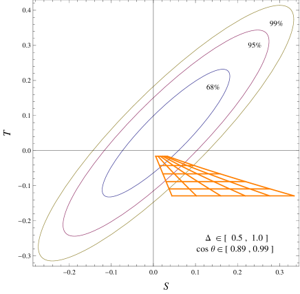
Figure 1: Contour plot for the S and T parameters counting the IR logarithmic contribution and UV resonance effects at the 68% $(1\sigma)$, 95% $(2\sigma)$ and 99% $(3\sigma)$ confidence levels. we adopt the benchmark point $g_{a}=g_{\rho}=3.0$.

$$\Pi^{\prime}_{{W_{3}}B}(0) = -\left(\frac{s_{h}^{2}}{2g_{\rho}^{2}}-\frac{\Delta\,s_{h}^{2}}{2g_{a}^{2}}\right)\,,\,\Pi^{\prime}_{W^{+}W^{-}}(0)=\Pi^{\prime}_{W_{3}W_{3}}(0)=-\frac{g_{0}^{2}+g_{\rho}^{2}}{g_{0}^{2}g_{\rho}^{2}}+\left(\frac{s_{h}^{2}}{2g_{\rho}^{2}}-\frac{\Delta\,s_{h}^{2}}{2g_{a}^{2}}\right)$$

$$\Pi^{\prime}_{BB}(0) = -\frac{g_{0}^{\prime 2}+g_{\rho}^{2}}{g_{0}^{\prime 2}g_{\rho}^{2}}+\left(\frac{s_{h}^{2}}{2g_{\rho}^{2}}-\frac{\Delta\,s_{h}^{2}}{2g_{a}^{2}}\right)\,,\quad\Pi_{W^{+}W^{-}}(0)=\Pi_{W_{3}W_{3}}(0)=\frac{f^{2}}{4}s_{h}^{2}$$ (15)

Note that the additional identity $\Pi_{BB}(0)=-\Pi_{W_{3}B}(0)=\Pi_{W_{3}W_{3}}(0)$ will ensure the electromagnetic gauge invariance. In our analysis, we are going to adopt the notation in Ref. [12], which are rescaled by $S=4s_{w}^{2}\hat{S}/\alpha$ and $T=\hat{T}/\alpha$ compared with the notation employed in Ref. [13]. Therefore including the resonance contribution, the deviations of $S$, $T$ and $U$ parameters from their SM evaluations are:

$$\Delta S=-16\pi\cdot\Pi^{\prime}_{W_{3}B}(0)=8\pi\left(\frac{s_{h}^{2}}{g_{\rho}^{2}}-\frac{\Delta\,s_{h}^{2}}{g_{a}^{2}}\right)\,,\qquad\Delta T=\Delta U=0\,$$ (16)

Considering the gauge sector exclusively, another calculable source is the infrared (IR) contribution, which comes from the reduced gauge couplings with Higgs boson [14].

$$\Delta{S_{IR}} = \frac{1}{6\pi}\left[s_{h}^{2}\log\left(\frac{\Lambda}{m_{h}}\right)+\log\left(\frac{m_{h}}{m_{h,ref}}\right)\right]\,,$$ (17)

$$\Delta{T_{IR}} = -\frac{3}{8\pi c_{w}^{2}}\left[s_{h}^{2}\log\left(\frac{\Lambda}{m_{h}}\right)+\log\left(\frac{m_{h}}{m_{h,ref}}\right)\right]$$ (18)

where the effective cut-off is defined as $\Lambda=4\pi f$. Other UV contribution to $S$ and $T$ incorporates the effects at the one-loop level from higher dimensional operators in the chiral expansion, which is possible to make some tuning to the IR contribution given that it is not sensitive to the composite scale $\Lambda$ [15]. Therefore ambiguarity exists for the oblique parameters without UV completing the effective theory. Extra calculable corrections to oblique parameters arise out of vector-like composite fermions, whose influence can be analyzed using the equations in Ref. [16]. At the one-loop level, composite fermion contribution to the $T$ parameter depends on the quantum number assignments in $SU(2)\times U(1)$, even though controled by its coupling to SM gauge bosons. For singlet and doublet vector-like fermions, we expect to get substantially positive contribution to the $T$ parameter and compensate the negative contribution from the infrared part in Eq.[18]. Since the $S$ parameter is mostly positive under the condition $0<\Delta<1$, a positive $T$ parameter (from vector-like fermions) is prefered to make the theory more compatible with the electroweak precison test.

As a rough estimate, we will just combine the results from Eq.[16- 18] to interpret the bound imposed on relevant parameters. The experimental values for $S$ and $T$ (leaving $U$ to be free) at $1\sigma$ deviation are:

$$S=0.03\pm 0.10\,,\quad T=0.05\pm 0.12$$ (19)

with the correlation coefficient set to be $0.89$ and the Higgs reference mass taken as $m_{h,ref}=126.0$ GeV. The lines in Fig. [1] show an important bound on the parameter space $(\Delta,\cos\theta)$ in this model from present electroweak precision data. For an input value $\Delta=0.5$, it is demanded $\cos\theta\in(0.97,1]$ to be consistent with electroweak precision measurement at $99\%$ C.L.. While we increase the value of $\Delta$, indicating more interplay between electroweak gauge bosons and axial fields, the stringent constraint from $S$ parameter will be relieved. As we can see with another input value $\Delta=1.0$, a larger fraction of region is permitted, i.e. $\cos\theta\in(0.91,1]$ at the $99\%$ C.L.

4 Higgs-Z-photon coupling

The model independent approach to discuss the Higgs phenomenology is adopting Effective Field Theory, through parameterizing the couplings of Higgs bosons with gauge bosons and fermions, deviations from new physics are accounted through the small corrections to the overall scaling factors [17]. Here we are going to employ the same effective Lagrangian used in the previous paper [18].

$$\mathcal{L}_{eff} = a_{W}\frac{2m_{W}^{2}}{v}h^{0}W_{\mu}^{+}W_{\mu}^{-}+a_{Z}\frac{m_{Z}^{2}}{v}h^{0}Z_{\mu}Z_{\mu}+c_{\rho}\frac{2m_{\rho}^{2}}{v}h^{0}\rho_{L\mu}^{+}\rho_{L\mu}^{-}+c_{a}\frac{2m_{a}^{2}}{v}h^{0}a_{\mu}^{+}a_{\mu}^{-}$$ (20)

$$+ c_{aW}\frac{m_{a}^{2}}{v}h^{0}\left(W_{\mu}^{+}a_{\mu}^{-}+W_{\mu}^{-}a_{\mu}^{+}\right)+c_{a\rho_{L}}\frac{m_{a}^{2}}{v}h^{0}\left(\rho_{L\mu}^{+}a_{\mu}^{-}+\rho_{L\mu}^{-}a_{\mu}^{+}\right)$$

$$+ {c_{f}}\left(\frac{m_{f}}{v}\bar{f}f\right)h_{0}+c_{\gamma}~{}\frac{\alpha}{8\pi v}h^{0}A^{\mu\nu}A_{\mu\nu}+c_{Z\gamma}\frac{\alpha}{4\pi v}h^{0}Z^{\mu\nu}A_{\mu\nu}$$

After rotating into the mass eigenstates and keeping the terms only at the leading order of $g_{0}/g_{\rho}$, $g_{0}^{\prime}/g_{\rho}$ and $\xi$, we get the modified Higgs couplings with various gauge bosons, i.e. $W_{\mu}^{\pm},Z_{\mu}$, $a_{\mu}^{\hat{i}}$ and $\rho_{\mu}^{a_{L},a_{R}}$ at the tree level:

$$a_{W} = \cos\theta+\frac{g_{0}^{2}\xi}{2g_{\rho}^{2}}\frac{m_{\rho}^{2}}{m_{W}^{2}}-\frac{\Delta^{2}g_{0}^{2}\xi}{2g_{\rho}^{2}}\frac{m_{a}^{2}}{m_{W}^{2}}\,$$

$$c_{a} = \frac{\Delta^{2}\xi g_{0}^{2}\left(m_{\rho}^{2}-m_{a}^{2}\right)}{2\left(g_{0}^{2}m_{\rho}^{2}+g_{\rho}^{2}(m_{\rho}^{2}-m_{a}^{2})\right)}\,$$

$$c_{\rho} = -\frac{g_{0}^{2}\xi}{2g_{\rho}^{2}}+\frac{\Delta^{2}\xi g_{0}^{4}m_{a}^{4}}{2g_{\rho}^{2}m_{\rho}^{2}\left(g_{0}^{2}m_{\rho}^{2}+g_{\rho}^{2}(m_{\rho}^{2}-m_{a}^{2})\right)}\,$$

$$a_{Z} = \cos\theta+\frac{\left(g_{0}^{2}+g_{0}^{\prime 2}\right)m_{\rho}^{2}\xi}{2g_{\rho}^{2}m_{Z}^{2}}-\frac{\Delta^{2}(g_{0}^{2}+g_{0}^{\prime 2})m_{a}^{2}\xi}{2g_{\rho}^{2}m_{Z}^{2}}$$ (21)

while the leading non-diagonal Higgs couplings appear at the $\xi^{1/2}$ order:

$$c_{aW}=\frac{\Delta}{\sqrt{2}}\frac{g_{0}}{g_{\rho}}\xi^{1/2}\,,\qquad c_{a\rho_{L}}=\frac{\Delta}{\sqrt{2}}\frac{g_{0}^{2}}{g_{\rho}^{2}}\xi^{1/2}$$ (22)

Due to the mixing from Eq.[10-11], non-diagonal gauge couplings with one $a_{\mu}^{\pm}$ involved occur at the $\xi^{1/2}$ order. In fact there are also non-diagonal gauge couplings with one $\rho_{L}^{\pm}$ involved which will appear at the $\xi$ order after rotating into the mass basis is performed. Hence the effects from the $\xi$ order vertexes could be safely ignored since they only lead to higher order correction. In the following discussion, we take a further simplification, $m_{a}=m_{\rho}$, which would imply that there is no Higgs coupling to two axial fields, i.e. $c_{a}=0$, under such an assumption. Albeit the mass of axial resonance is usually expected to be slightly heavier than the mass of vector resonance, i.e. $m_{a}>m_{\rho}$, we have checked that in such a situation the relevant phenomenology discussed in this section will not be altered too much. It is worthwhile for us to show that including non-diagonal couplings exclusively leads to a gauge-invariant contribution for the form factor $c_{Z\gamma}^{(1)}$.

Figure 2: (a) triangle feyndiagram with one axial resonance, (b) triangle feyndiagram with two axial resonances , (c) quartic feyndiagram with one axial resonance.

The generic non-diagonal trilinear and quartic gauge self couplings can be put in the following way:

$$\mathcal{L}_{ZV_{1}V_{2}} = (-i\,e\,\cot\theta_{w})\,c_{ZV_{1}V_{2}}\bigg{(}\partial_{\mu}Z_{\nu}V_{2,\mu}^{+}V_{1,\nu}^{-}+\partial_{\mu}V_{2,\nu}^{+}V_{1,\mu}^{-}Z_{\nu}+\partial_{\mu}V_{1,\nu}^{-}Z_{\mu}V_{2,\nu}^{+}$$ (23)

$$+ \partial_{\mu}Z_{\nu}V_{2,\nu}^{-}V_{1,\mu}^{+}+\partial_{\mu}V_{2,\nu}^{-}V_{1,\nu}^{+}Z_{\mu}+\partial_{\mu}V_{1,\nu}^{+}Z_{\nu}V_{2,\mu}^{-}-\left(\mu\leftrightarrow\nu\right)\bigg{)}$$

$$\mathcal{L}_{AZV_{1}V_{2}} = (e^{2}\,\cot\theta_{w})\,c_{ZV_{1}V_{2}}\bigg{(}2~{}Z_{\mu}A_{\mu}V^{+}_{2,\nu}V^{-}_{1,\nu}-Z_{\mu}A_{\nu}V^{+}_{2,\mu}V^{-}_{1,\nu}-Z_{\mu}A_{\nu}V^{+}_{2,\nu}V^{-}_{1,\mu}$$ (24)

$$+ 2~{}Z_{\mu}A_{\mu}V^{-}_{2,\nu}V^{+}_{1,\nu}-Z_{\mu}A_{\nu}V^{-}_{2,\nu}V^{+}_{1,\mu}-Z_{\mu}A_{\nu}V^{-}_{2,\mu}V^{+}_{1,\nu}\bigg{)}$$

where the index exchange $\left(\mu\leftrightarrow\nu\right)$ refers to the last two variables, and one way to check the validity is that the Lagrangian need to be self-conjugate. Therefore in our model setup, using the information provided in Eq.[12-13], at the leading order expansion, non-diagonal gauge couplings $c_{ZaW}$ and $c_{Za\rho_{L}}$ are expressed as:

$$c_{ZaW}=\frac{\Delta}{\sqrt{2}}\frac{g_{0}^{2}+g_{0}^{\prime 2}}{2g_{0}g_{\rho}}{\xi^{1/2}}\,,\qquad c_{Za\rho_{L}}=-\frac{\Delta}{\sqrt{2}}\frac{\left(g_{0}^{2}+g_{0}^{\prime 2}\right)}{2g_{0}^{2}}\,\xi^{1/2}\,$$ (25)

To calculate the amplitude for $h^{0}\to Z\gamma$, it is simply to add up the three diagrams illustrated in Fig. [2] and times a symmetry factor of two to account for another three equivalent diagrams with the simultaneous external and internal fields exchange: i.e. $Z_{\mu}\leftrightarrow A_{\mu}$ and $W_{\mu}^{\pm}\leftrightarrow a_{\mu}^{\pm}$. As we put all the external particles to be on shell, the amplitude can be organized into a gauge invariant form:

$$M({h^{0}}\to Z\gamma)=2\cdot\left(M^{(a)}+M^{(b)}+M^{(c)}\right)$$ (26)

$$= \frac{-i\,e^{2}}{8\pi^{2}v}\cdot(2~{}c_{V_{1}V_{2}}\,c_{ZV_{1}V_{2}})~{}c_{Z\gamma}^{(1)}(m_{1},m_{2})\,\left({{g^{\mu\nu}}{k_{1}}\cdot{k_{2}}-k_{1}^{\mu}k_{2}^{\nu}}\right)\,\varepsilon_{\mu}^{*}({k_{1}})\varepsilon_{\nu}^{*}({k_{2}})$$

Putting everything together, the form factor for $H$-$Z$-$\gamma$ vertex contains the dominating contribution from both the fermion sector and the gauge sector:

$$c_{Z\gamma} = c_{t}\,N_{c}\,\frac{(Q_{t}-4Q_{t}^{2}s_{w}^{2})}{s_{w}c_{w}}\,m_{t}^{2}\,c_{Z\gamma}^{f}\,(m_{t})+a_{W}\,c_{Z\gamma}^{(0)}\,(m_{W})$$ (27)

$$+ \left(c_{\rho}+2\,c_{a\rho_{L}}\,c_{Za\rho_{L}}\right)c_{Z\gamma}^{(0)}{(m_{a})}+2\,c_{aW}\,c_{ZaW}\,c_{Z\gamma}^{(1)}\,(m_{W},m_{a})$$

with each piece of $c_{Z\gamma}$ being expressed by the one-loop scalar and vector three point functions $C_{0}$ and $C_{2}$ defined in [19]:

$$c_{Z\gamma}^{f}\,(m_{t}) = 4~{}C_{2}(m_{h}^{2},m_{Z}^{2},0,m_{t}^{2},m_{t}^{2},m_{t}^{2})+C_{0}\left(m_{h}^{2},m_{Z}^{2},0,m_{t}^{2},m_{t}^{2},m_{t}^{2}\right)$$ (28)

$$c_{Z\gamma}^{(0)}\,(m_{1}) = \cot\theta_{w}\cdot\bigg{[}2\left(\frac{m_{h}^{2}}{m_{1}^{2}}\,\left({m_{Z}^{2}-2m_{1}^{2}}\right)+2\,(m_{Z}^{2}-6m_{1}^{2})\right)C_{2}(m_{h}^{2},m_{Z}^{2},0,m_{1}^{2},m_{1}^{2},m_{1}^{2})$$ (29)

$$+ 4\left(m_{Z}^{2}-4m_{1}^{2}\right)\cdot C_{0}\left(m_{h}^{2},m_{Z}^{2},0,m_{1}^{2},m_{1}^{2},m_{1}^{2}\right)\bigg{]}$$

$$c_{Z\gamma}^{(1)}\,(m_{1},m_{2}) = \cot\theta_{w}\cdot\frac{m_{2}^{2}}{m_{1}^{2}}\cdot\bigg{[}\left(\left({\frac{m_{h}^{2}}{m_{2}^{2}}+\frac{m_{1}^{2}}{m_{2}^{2}}+1}\right)\left(m_{Z}^{2}-m_{2}^{2}-m_{1}^{2}\right)-8m_{1}^{2}\right)$$ (30)

$$\cdot \bigg{(}C_{2}\left(m_{h}^{2},m_{Z}^{2},0,m_{1}^{2},m_{2}^{2},m_{1}^{2}\right)+C_{2}\left(m_{h}^{2},m_{Z}^{2},0,m_{2}^{2},m_{1}^{2},m_{2}^{2}\right)\bigg{)}$$

$$+ 2\left(\frac{m_{1}^{2}}{m_{2}^{2}}\left(m_{Z}^{2}-m_{1}^{2}-3m_{2}^{2}\right)\right)\cdot C_{0}\left(m_{h}^{2},m_{Z}^{2},0,m_{1}^{2},m_{2}^{2},m_{1}^{2}\right)$$

$$+ 2\left(m_{Z}^{2}-3m_{1}^{2}-m_{2}^{2}\right)\cdot C_{0}\left(m_{h}^{2},m_{Z}^{2},0,m_{2}^{2},m_{1}^{2},m_{2}^{2}\right)\bigg{]}$$

where the $C_{2}$ function in the expression of $c_{Z\gamma}^{(0)}$ and the combination of $C_{2}$ functions with different masses in the expression of $c_{Z\gamma}^{(1)}$ can be recasted into Passarino-Veltman functions $B_{0}$ and $C_{0}$:

$$C_{2}\left(m_{h}^{2},m_{Z}^{2},0,m_{1}^{2},m_{1}^{2},m_{1}^{2}\right)$$ (31)

$$= \frac{m_{Z}^{2}}{2\left({m_{Z}^{2}-m_{h}^{2}}\right)^{2}}\bigg{(}B_{0}\left({m_{Z}^{2},m_{1}^{2},m_{1}^{2}}\right)-B_{0}\left({m_{h}^{2},m_{1}^{2},m_{1}^{2}}\right)\bigg{)}$$

$$+ \frac{1}{2\left({m_{Z}^{2}-m_{h}^{2}}\right)}+\frac{m^{2}}{\left(m_{Z}^{2}-m_{h}^{2}\right)}C_{0}\left(m_{h}^{2},m_{Z}^{2},0,m_{1}^{2},m_{1}^{2},m_{1}^{2}\right)$$

$$C_{2}\left(m_{h}^{2},m_{Z}^{2},0,m_{1}^{2},m_{2}^{2},m_{1}^{2}\right)+C_{2}\left(m_{h}^{2},m_{Z}^{2},0,m_{2}^{2},m_{1}^{2},m_{2}^{2}\right)$$ (32)

$$= \frac{m_{Z}^{2}}{\left({m_{Z}^{2}-m_{h}^{2}}\right)^{2}}\bigg{(}B_{0}\left({m_{Z}^{2},m_{2}^{2},m_{1}^{2}}\right)-B_{0}\left({m_{h}^{2},m_{2}^{2},m_{1}^{2}}\right)\bigg{)}$$

$$+ \frac{1}{\left({m_{Z}^{2}-m_{h}^{2}}\right)}+\frac{m_{1}^{2}}{\left(m_{Z}^{2}-m_{h}^{2}\right)}C_{0}\left(m_{h}^{2},m_{Z}^{2},0,m_{1}^{2},m_{2}^{2},m_{1}^{2}\right)$$

$$+ \frac{m_{2}^{2}}{\left(m_{Z}^{2}-m_{h}^{2}\right)}C_{0}\left(m_{h}^{2},m_{Z}^{2},0,m_{2}^{2},m_{1}^{2},m_{2}^{2}\right)$$

Notice that in the limit of $m_{2}=m_{1}$, our new form factor $c_{Z\gamma}^{(1)}$ will reduce exactly to the $W$ gauge bosons mediated SM contribution $c_{Z\gamma}^{(0)}$ [20]. Since the mass of axial resonance $m_{a}$ is much larger than the mass in $(m_{h},m_{Z},m_{W})$, it is meaningful to take the heavy mass limit expansion for $c_{Z\gamma}^{(0)}(m_{a})$ and $c_{Z\gamma}^{(1)}(m_{W},m_{a})$, which , to the leading orders, could be asymptoted by the following approximations:

$$c_{Z\gamma}^{(0)}(m_{a}) \simeq \cot\theta_{w}\cdot\bigg{(}7+\frac{\left(11m_{h}^{2}-37m_{Z}^{2}\right)}{30m_{a}^{2}}\bigg{)}+\mathcal{O}\left(\frac{1}{m_{a}^{4}}\right)$$

$$c_{Z\gamma}^{(1)}(m_{W},m_{a}) \simeq \cot\theta_{w}\cdot\bigg{(}\frac{7m_{a}^{2}}{4m_{W}^{2}}+\frac{9}{2}\log\left(\frac{m_{a}^{2}}{m_{W}^{2}}\right)+\frac{5m_{h}^{2}-47m_{Z}^{2}-45m_{W}^{2}}{36m_{W}^{2}}\bigg{)}$$ (33)

$$+ \mathcal{O}\left(\frac{1}{m_{a}^{2}}\log\left(\frac{m_{a}^{2}}{m_{W}^{2}}\right)\right)$$

It should be mentioned that the non-diagonal contribution mildly makes up around $5\%$-$10\%$ contribution to the total $c_{Z\gamma}$ form factor provided that $m_{a}$ is around the TeV scale and it interferes with the SM portion constructively. Accordingly we are going to conclude that substantial correction is induced by the shift in $a_{W}$ after we take into account the mixing effects.

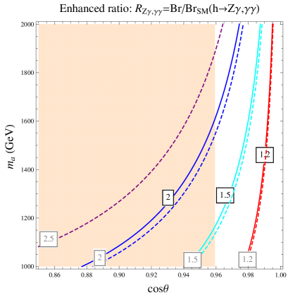
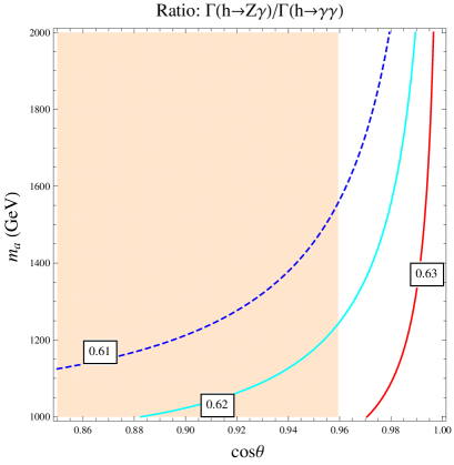
Figure 3: Left Contour: signal strengths for $Z\gamma$ mode(solid line) and $\gamma\gamma$ mode (dashed line) in the $(m_{a},\cos\theta)$ plane. The purple dashed line shows the upper bound measured by ATLAS at $68\%$ confidence level. Right Contour: the decay width ratio between $Z\gamma$ mode and $\gamma\gamma$ mode in the $(m_{a},\cos\theta)$ plane. The condition $\Delta=0.5$ is imposed. The light orange region is excluded by the EWPT requirement $S<0.13$.

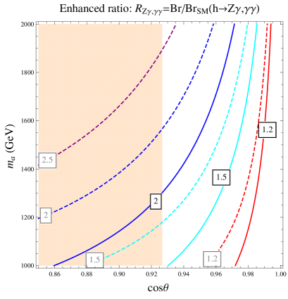
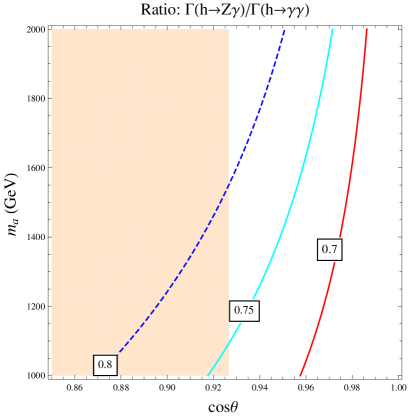
Figure 4: Left Contour: signal strengths for $Z\gamma$ mode (solid line) and $\gamma\gamma$ mode (dashed line) in the $(m_{a},\cos\theta)$ plane. The purple dashed line shows the upper bound measured by ATLAS at $68\%$ confidence level. Right Contour: the decay width ratio between $Z\gamma$ mode and $\gamma\gamma$ mode in the $(m_{a},\cos\theta)$ plane. The condition $\Delta=0.75$ is imposed. The light orange region is excluded by the EWPT requirement $S<0.13$.

Now we proceed to analyze the process of $h^{0}\to Z\gamma$ and compare it with the experimentally better measured process $h^{0}\to\gamma\gamma$. In terms of the form factor $c_{Z\gamma}$ and the rescaled branching ratio for each Higgs decay mode, it is convenient to define the signal strength $R_{Z\gamma}$, which is one of the measurable properties at the LHC. Let us solely consider the gluon fusion process, where the ratio for the production cross sections is $\sigma/\sigma_{sm}=c_{t}^{2}$, i.e. the one in composite Higgs model divided by its SM expectation. Then when assuming $c_{t}=1$, we have:

$$R_{Z\gamma}=\frac{|c_{Z\gamma}/c_{Z\gamma}^{sm}|^{2}}{a_{W}^{2}Br_{sm}^{(WW^{*})}+a_{Z}^{2}Br_{sm}^{(ZZ^{*})}+|c_{\gamma\gamma}/c_{\gamma\gamma}^{sm}|^{2}Br_{sm}^{(\gamma\gamma)}+|c_{Z\gamma}/c_{Z\gamma}^{sm}|^{2}Br_{sm}^{(Z\gamma)}+\cdots}\,,$$ (34)

and for the diphton process, the signal strength $R_{\gamma\gamma}$ is calculated in analogous way by substituting $|c_{Z\gamma}/c_{Z\gamma}^{sm}|^{2}$ with $|c_{\gamma\gamma}/c_{\gamma\gamma}^{sm}|^{2}$ in the numerator, where the analytic expression for $c_{\gamma\gamma}$ in this model has already been given in [18]. Since $h^{0}\to Z\gamma$ and $h^{0}\to\gamma\gamma$ are correlated to each other due to the EW symmetry breaking, following the proposal in [6], we define a useful parameter, the decay width ratio between these two modes, to measure the degree of correlation :

$$\frac{\Gamma(h^{0}\to Z\gamma)}{\Gamma(h^{0}\to\gamma\gamma)}=2\cdot\bigg{|}\frac{c_{Z\gamma}}{c_{\gamma\gamma}}\bigg{|}^{2}\frac{(m_{h}^{2}-m_{Z}^{2})^{3}}{m_{h}^{6}}\,.$$ (35)

Contours in Fig. [3] quantitatively show behaviors of signal strengths $R_{Z\gamma}$, $R_{\gamma\gamma}$ and the decay width ratio $\frac{\displaystyle\Gamma(h^{0}\to Z\gamma)}{\displaystyle\Gamma(h^{0}\to\gamma\gamma)}$ in the plane of $(m_{a},\cos\theta)$, with other parameters fixed: $g_{\rho}=g_{a}=3.0$ and $\Delta=0.5$. As we can see, the stringent EWPT constraint comes from the $S$ parameter. Obviously the one dimension $68\%$ C.L. bound $S<0.13$ translates to be a condition $\cos\theta>0.96$. The left contour shows that a signal strength as much as $R_{Z\gamma}\approx 1.5$ is possible to be achieved in a sizable portion of parameter region when we demand $m_{a}>1.2~{}\mbox{TeV}$ and $\cos\theta>0.96$. For comparison it is shown with the dashed lines that $R_{\gamma\gamma}$ is slightly larger for a given point at the $(m_{a},\cos\theta)$ plane. On experimental side, the most recent measurement at ATLAS reported an enhancement in diphoton signal strength to be $1.8^{+0.71}_{-0.59}$ with the errors linearly added  [21]. Therefore the upper bound $R_{\gamma\gamma}\sim 2.5$ at least provides certain constraint on the parameter space as indicated by the dashed purple line in the left contour. Notice that since in our model $m_{a}$ is not correlated to $\cos\theta\equiv\cos(v/f)$, the decoupling of spin-$1$ resonance will only happen as $f$ is pushed into $\infty$ (i.e. $\cos\theta$ goes into $1$), and in such a limit the Standard Model is recovered. On the other hand, the right contour illustrates the correlation between $Z\gamma$ mode and $\gamma\gamma$ mode. The value for this ratio in the SM is $\frac{\displaystyle\Gamma_{Z\gamma,sm}}{\displaystyle\Gamma_{\gamma\gamma,sm}}=0.636$. Positive deviation from this value roughly indicates that $R_{Z\gamma}$ would be larger in contrast to $R_{\gamma\gamma}$, while negative deviation implies the other situation. Under the condition $\Delta=0.5$, the ratio is generally smaller than its SM value, and when we decrease $\cos\theta$ and increase $m_{a}$, the ratio will be further reduced. This verifies the exact trend that we observe from the left contour.

In Fig. [4], we choose another benchmark point $g_{\rho}=g_{a}=3.0$ and $\Delta=0.75$ and draw the contours in the same manner. In this case, when we demand $S<0.13$, the lowest allowed value of $\cos\theta$ is tuned to be $0.92$ such that we get more EWPT applicable parameter space. This gain is achieved with the deduction in the enhancement rates for $h^{0}\to Z\gamma,\gamma\gamma$. However more enhancement is found for the $Z\gamma$ mode rather than for the $\gamma\gamma$ mode, compared with the former case. An inverse pattern is similarly displayed in the correlation contour, i.e. with smaller $\cos\theta$ and bigger $m_{a}$, the ratio will be instead increased. Moreover the ratio tends to be larger than in the SM provided that the value of $\Delta$ is close enough to $1.0$.

5 Conclusion

In this paper we discuss the circumstance that axial resonances and vector resonances are present in the low energy particle spectrum of composite Higgs model. As we know that in a general composite Higgs model, we need vector resonance to restore the perturbative unitarity till the effective cut off scale. However the solely including of vector resonance on the other hand increases the $S$ parameter and potentially renders it to be too big. In the scenario that composite Higgs emerging as a pNGB from a spontaneously broken global symmetry, a custodial symmetry is usually imposed to protect the $T$ parameter, whereas the deviation in the $S$ parameter is measured by $v^{2}/f^{2}$ without being suppressed by one loop factor, therefore it would cause a tension with the electroweak precision measurement since we demand the composite scale $4\pi f\sim\mathcal{O}(10~{}\mbox{TeV})$ in order to reduce the amount of fine tuning. One solution to cure this problem is to introduce axial resonance as it will partially relieve the stringent constraint and pull the $S$ parameter back to the origin point.

One crucial feature in a Composite Higgs Model is the partial compositeness of gauge bosons. The nonlinear realization modifies the Higgs couplings via the strong dynamics, with the consequence that the correction may not be too much small. We calculate the signal strength for $h^{0}\to Z\gamma$ in the context of a truncated effective theory, especially including the non-diagonal gauge contribution for accuracy and we find out that in most EWPT allowed region, the signal strength for $Z\gamma$ could be enhanced as much as $50\%$. It eventually turns out that the correlation between the $Z\gamma$ and $\gamma\gamma$ modes in our model is relatively similar to the SM expectation. Furthermore vector and axial resonances lead to simultanous enhancement for both signals. Nevertheless the result should be testable in future LHC experiments and precise measurement of $H$-$Z$-$\gamma$ vertex would help to distinguish new physics scenarios.

Appendix A Sigma Field in Unitary Gauge

Here we collect all the $SO(5)$ generators such that we can calculate the sigma matrix explicitly.

$$T_{ij}^{\hat{a}} = \frac{i}{{\sqrt{2}}}\left[{\delta_{i}^{\hat{a}}\delta_{j}^{5}-\delta_{j}^{\hat{a}}\delta_{i}^{5}}\right]$$

$$T_{L,ij}^{a} = -\frac{i}{2}\left[{\frac{1}{2}{\varepsilon^{abc}}\left({\delta_{i}^{b}\delta_{j}^{c}-\delta_{j}^{b}\delta_{i}^{c}}\right)+\left({\delta_{i}^{a}\delta_{j}^{4}-\delta_{j}^{a}\delta_{i}^{4}}\right)}\right]$$

$$T_{R,ij}^{a} = -\frac{i}{2}\left[{\frac{1}{2}{\varepsilon^{abc}}\left({\delta_{i}^{b}\delta_{j}^{c}-\delta_{j}^{b}\delta_{i}^{c}}\right)-\left({\delta_{i}^{a}\delta_{j}^{4}-\delta_{j}^{a}\delta_{i}^{4}}\right)}\right]$$ (36)

where $T^{\hat{a}}$ with $\hat{a}=1,2,3,4$ are generators in the coset space $SO(5)/SO(4)$, while $T^{a}_{L,R}$ (denoted as $T^{a_{L},a_{R}}$ somewhere) with $a=1,2,3$ are generators in the unbroken subgroup $SU(2)_{L}\times SU(2)_{R}$ respectively. Since the coset space $SO(5)/SO(4)$ is symmetric, an automorphism of the algebra will change the sign of the broken generators: $T^{\hat{a}}\to-T^{\hat{a}}$. However without conducting a field transformation $\pi^{\hat{a}}\to-\pi^{\hat{a}}$, the choice of sign for the broken generators will not alter the CCWZ objects.

In the unitary gauge, since the other three pion fields are eaten by the external $W$ and $B$ gauge bosons, only the Higgs field enters into the parameterization $\pi^{\hat{a}}=(0,0,0,h^{0})$, and the sigma matrix $U=\mbox{exp}(i\sqrt{2}\pi^{\hat{a}}T^{\hat{a}}/f)$ is represented by:

$$U=\left(\begin{array}[]{ccc}I_{3\times 3}&&\\ &\cos\frac{h^{0}}{f}&-\sin\frac{h^{0}}{f}\\ &\sin\frac{h^{0}}{f}&\cos\frac{h^{0}}{f}\end{array}\right)$$ (40)

Thus for the CCWZ objects $d_{\mu}^{a}$ and $E_{\mu}^{a_{L,R}}$, they have the following compact forms:

$$d_{\mu} = -\frac{\sqrt{2}}{f}\partial_{\mu}h^{0}\,T^{\hat{4}}+\frac{1}{\sqrt{2}}\sin\left(\frac{h^{0}}{f}\right)\left(g_{0}\tilde{W}_{\mu}^{a}-g_{0}^{\prime}\tilde{B}_{\mu}\delta^{a3}\right)\delta^{a\hat{i}}\,T^{\hat{i}}\,$$ (41)

$$E_{\mu} = \left(g_{0}\tilde{W}_{\mu}^{a}T_{L}^{a}+g_{0}^{\prime}\tilde{B}_{\mu}T_{R}^{3}\right)-\sin^{2}\left(\frac{h^{0}}{2f}\right)\left(g_{0}\tilde{W}_{\mu}^{a}-g_{0}^{\prime}\tilde{B}_{\mu}\delta^{a3}\right)(T_{L}^{a}-T_{R}^{a})$$ (42)

Obviously they will translate into the previous notations used in Eq.[2], through the leading order chiral expansion.

References

- [1] G. Aad et al. [ATLAS Collaboration], Phys. Lett. B 716 (2012) 1 arXiv:1207.7214 [hep-ex]; S. Chatrchyan et al. [CMS Collaboration], Phys. Lett. B 716 (2012) 30 arXiv:1207.7235 [hep-ex].
- [2] R. Contino, Y. Nomura and A. Pomarol, Nucl. Phys. B 671, 148 (2003) [hep-ph/0306259]; K. Agashe, R. Contino and A. Pomarol, Nucl. Phys. B 719, 165 (2005) [hep-ph/0412089]; C. Anastasiou, E. Furlan and J. Santiago, Phys. Rev. D 79, 075003 (2009) arXiv:0901.2117 [hep-ph]; G. Panico and A. Wulzer, JHEP 1109, 135 (2011) arXiv:1106.2719 [hep-ph]; S. De Curtis, M. Redi and A. Tesi, JHEP 1204, 042 (2012) arXiv:1110.1613 [hep-ph];
- [3] J. S. Gainer, W. -Y. Keung, I. Low and P. Schwaller, Phys. Rev. D 86, 033010 (2012) arXiv:1112.1405 [hep-ph]
- [4] M. Carena, I. Low and C. E. M. Wagner, JHEP 1208, 060 (2012) arXiv:1206.1082 [hep-ph];
- [5] A. Djouadi, V. Driesen, W. Hollik and A. Kraft, Eur. Phys. J. C 1, 163 (1998) [hep-ph/9701342].
- [6] C. -W. Chiang and K. Yagyu, arXiv:1207.1065 [hep-ph].
- [7] S. R. Coleman, J. Wess and B. Zumino, Phys. Rev. 177, 2239 (1969); C. G. Callan Jr., S. R. Coleman, J. Wess and B. Zumino, Phys. Rev. 177, 2247 (1969).
- [8] R. Contino, D. Marzocca, D. Pappadopulo and R. Rattazzi, JHEP 1110, 081 (2011) [arXiv:1109.1570 [hep-ph]].
- [9] D. Marzocca, M. Serone and J. Shu, JHEP 1208 (2012) 013 [arXiv:1205.0770 [hep-ph]].
- [10] B. Bellazzini, C. Csaki, J. Hubisz, J. Serra and J. Terning, JHEP 1211 (2012) 003 arXiv:1205.4032 [hep-ph].
- [11] D. Barducci, A. Belyaev, S. De Curtis, S. Moretti and G. M. Pruna, JHEP 1304, 152 (2013) [arXiv:1210.2927 [hep-ph]].
- [12] M. E. Peskin and T. Takeuchi, Phys. Rev. Lett. 65, 964 (1990); Phys. Rev. D 46, 381 (1992);
- [13] R. Barbieri, A. Pomarol, R. Rattazzi and A. Strumia, Nucl. Phys. B 703, 127 (2004) [hep-ph/0405040].
- [14] R. Barbieri, B. Bellazzini, V. S. Rychkov and A. Varagnolo, Phys. Rev. D 76, 115008 (2007) [arXiv:0706.0432 [hep-ph]].
- [15] A. Pich, I. Rosell and J. J. Sanz-Cillero, arXiv:1212.6769 [hep-ph].
- [16] L. Lavoura and J. P. Silva, Phys. Rev. D 47 (1993) 2046; H. Cai, JHEP 1302, 104 (2013) arXiv:1210.5200 [hep-ph].
- [17] G. Cacciapaglia, A. Deandrea, G. D. La Rochelle and J. -B. Flament, arXiv:1210.8120 [hep-ph].
- [18] H. Cai, Phys. Rev. D 88, 035018 (2013) arXiv:1303.3833 [hep-ph].
- [19] G. ’t Hooft and M. J. G. Veltman, Nucl. Phys. B 153, 365 (1979); G. Passarino and M. J. G. Veltman, Nucl. Phys. B 160, 151 (1979); A. Denner, Fortsch. Phys. 41, 307 (1993) arXiv:0709.1075 [hep-ph]
- [20] F. Wilczek, Phys. Rev. Lett. 39 (1977) 1304; R.N. Cahn, M.S. Chanowitz and N. Fleishon, Phys. Lett. B82 (1979) 113; L. Bergstrom and G. Hulth, Nucl. Phys. B259 (1985) 137.
- [21] The ATLAS Collaboration, ATLAS-CONF-2012-168.