Exact band structures for 1D superlattices beyond the tight-binding approximation

Abstract

The band structures describing non-interacting particles in one-dimensional superlattices of arbitrary periodicity are obtained by an analytical diagonalization of the Hamiltonian without adopting the popular tight-binding approximation. The results are compared with those of the tight-binding approximation. In this way, a quantitative prediction of the validity and failure of the tight-binding approximation becomes possible. In particular, it is demonstrated that in contrast to the prediction of the tight-binding approximation the central energy bands do not touch for periodicities $\tau$ of the lattice where $\tau=4n$ and $n$ is an integer.

Introduction — The physics of optical lattices was studied intensely over the past ten years, starting with the first experimental realization in which ultracold atoms were trapped in the periodic potential generated by standing waves of laser light Greiner et al. (2002); Lewenstein et al. (2007); Bloch et al. (2008). They are still of experimental and theoretical interest due to the fact that both the lattice parameters (depth, spacing, and even overall geometry) and the atom-atom interaction can be experimentally tuned within large ranges. This permits the use of these systems as quantum simulators for, e. g., Hamiltonians of solid-state physics. Combined with the recently achieved single-site addressability (detection and manipulation) ultracold atoms (or molecules) in optical lattices are very promising candidates for a possible realization of quantum computers Jaksch et al. (1999). The usual approach adopted in the description of the physics in such uniform optical lattices is the Hubbard model using a tight-binding approximation (TBA) in which only next-neighbor hopping and a delta-function (on-site) interaction is considered.

Optical superlattices Jaksch et al. (1998); Sebby-Strabley et al. (2006); Fölling et al. (2007) are a variation of the uniform lattices and are obtained by a superposition of at least two different standing waves of laser light with different frequencies. The ratio $\tau$ of the adopted wavelengths equals the periodicity of the resulting superlattice. Such superlattices provide a possible realization of a quantum computer Anderlini et al. (2006); Mazza et al. (2012); Bloch et al. (2012). The Hamiltonian of non-interacting particles trapped in a superlattice was solved analytically within the TBA Rousseau et al. (2006). Such solutions are of great interest, since they provide a good approximation for the band structure in the weakly interacting limit. In fact, it is now experimentally possible to reduce or even turn off the effective interaction between the particles using Feshbach resonances Chin et al. (2010). Furthermore, especially analytical one-particle solutions can be the starting point for deriving perturbative or sometimes even exact results for interacting few- or even many-body systems. For example, exact solutions within the TBA for two interacting particles in a superlattice with periodicity 2 were found with an extended Bethe ansatz Valiente et al. (2010). Finally, part of the interest in one-dimensional systems stems from the fact that they provide the highest chances for finding analytical results Mattis (1993); Cazalilla et al. (2011). This is always very attractive from a general point of view and leads sometimes (via mapping) to analytical solutions of much more complicated problems.

In this work the band structure for an optical superlattice with arbitrary periodicity is obtained without adopting the TBA. Thus it generalizes the results obtained recently within the TBA Rousseau et al. (2006). While in the latter approximation the central energy bands were found to touch for all $\tau=4n$ where $n$ is an integer, the rigorous results obtained beyond the TBA show that this behavior is in reality modified and the bands do not touch. Besides this important qualitative difference, the present results provide also the possibility to study quantitatively the failure of the TBA in optical superlattices for flat lattices.

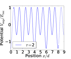
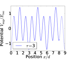
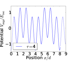
Figure 1: (Color online) Example superlattice potentials $V_{\mathrm{sup}}$ [Eq. (1)] for $V_{0}=E_{\mathrm{rec}},V_{1}=0.4E_{\mathrm{rec}}$, and different periodicities $\tau$.

Hamiltonian — In this work, a one-dimensional superlattice potential

$$V_{\mathrm{sup}}=V_{G}(x)+V_{M}(x)=-V_{0}\cos(2\pi x)-V_{1}\cos\left(\frac{2\pi x}{\tau}\right)$$ (1)

is considered which is a superposition of a standard lattice potential $V_{G}(x)$ and a modulation lattice $V_{M}(x)$ with periodicity $\tau$. The problem to be solved is related to the Hill equation Hill (1886); Olver et al. (2010). To the authors’ knowledge, only for the specific case of $\tau=2$ (Whittaker-Hill equation) a solution exists in literature, but even then only as an infinite Fourier-expansion with a recipe for calculating the coefficients. Here and in the following all lengths are given in units of the lattice spacing $d$. Hence, momenta are given in units of $d^{-1}$. The superlattice has $N$ lattice sites at integer values $x$ ranging from $0$ to $N-1$. Periodic boundary conditions are used. Examples for various types of optical superlattices are depicted in Fig. 1. The system is set up using low temperatures. Thus, there are $N$ one-particle states forming the Hilbert space $\mathcal{H}$ of the system which is called the 1. Bloch band. Without the modulation lattice, $V_{1}=0$, the system’s one-particle Hamiltonian would read $\hat{h}_{1}=-\frac{\hbar^{2}}{2M}\frac{\mathtt{d}^{2}}{\mathtt{d}x^{2}}-V_{0}\cos(2\pi\hat{x})$, where $M$ denotes the mass of the considered particles. In the following, all energies are given in units of the recoil energy $E_{\mathrm{rec}}=\frac{\pi^{2}\hbar^{2}}{2M}$. The eigenstates $\ket{k}$ and eigenenergies $\epsilon(k)$ of $\hat{h}_{1}$ are analytically well known. $\ket{k}$ are called Bloch states. Bloch’s theorem states that $\Psi_{k}(x):=\Braket{x}{k}=e^{ikx}u_{k}(x)$ where $u_{k}(x)$ is a periodic function in $x$. From this theorem and periodic boundary conditions $\Psi_{k}(x+N)=\Psi_{k}(x)$ follows that the $k$-quantum numbers, which represent the quasi momenta, are discrete,

$$k=\frac{2\pi}{N}s,\quad s\in\mathbb{Z}.$$ (2)

Furthermore, the $N$ Bloch states $\ket{k}$ with $k\in[-\pi,+\pi)$ form a complete and orthonormal basis of $\mathcal{H}$.

The Fourier transformation

$$\Ket{w}=\sum_{\ket{k}\in\mathcal{H}}\sqrt{\frac{1}{N}}e^{-ikw}\Ket{k}$$ (3)

defines the Wannier states $\ket{w}$ which also form a complete and orthonormal basis of $\mathcal{H}$ choosing $w$ in between $0$ and $N-1$. The absolute value square of the Wannier wave function $\Phi_{w}(x)=\Braket{x}{w}$ is depicted in Fig. 2.

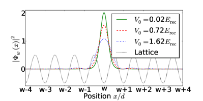
Figure 2: (Color online) Squared absolute values of the Wannier wave functions $|\Phi_{w}(x)|^{2}$ for a uniform optical lattice ($V_{1}=0$) with different $V_{0}$. For better readability, only a single optical lattice with arbitrary amplitude is shown (dotted line) to indicate the positions of the minima.

As can be seen, $\Phi_{w}(x)$ is well located at the lattice site $w$, especially for deep latices. From Eqs. (2) and (3) follow periodic boundary conditions for the Wannier states,

$$\Ket{w+N}=\Ket{w}.$$ (4)

In this basis, the Hamiltonian of the system is

$$\hat{H}=\sum_{ww^{\prime}}\mathcal{J}\left(w,w^{\prime}\right)\hat{a}^{\dagger}_{w}\hat{a}_{w^{\prime}},$$ (5)

with the matrix elements

$$\mathcal{J}\left(w,w^{\prime}\right) = \Braket{w}{\hat{T}+\hat{V}_{G}(\hat{x})+\hat{V}_{M}(\hat{x})}{w^{\prime}}$$ (6)

$$= \sum_{k}\frac{\epsilon(k)}{N}e^{ik(w-w^{\prime})}-$$

$$-V_{1}\int\textrm{d}x\cos\left(\frac{2\pi}{\tau}x\right)\Phi^{*}_{w}(x)\Phi_{w^{\prime}}(x)$$

and the annihilation and creation operators of Wannier states $\hat{a}_{w}$ and $\hat{a}^{\dagger}_{w}$, respectively, that fulfill the usual bosonic (fermionic) (anti-)commutator relations.

The TBA neglects all $\mathcal{J}\left(w,w^{\prime}\right)$ with $|w-w^{\prime}|>1$ and assumes a small overlap between different Wannier functions, $\left[\Phi_{w}^{*}(x)\Phi_{w^{\prime}}(x)\right]_{\mathrm{TBA}}=\delta_{ww^{\prime}}\delta(w-x)$. Then, the chemical potential $\mu_{0}:=\sum_{k}\frac{\epsilon(k)}{N}$ and the Hopping parameter $J:=-\sum_{k}\frac{\epsilon(k)}{N}e^{ik}$ can be defined and the Hamiltonian in TBA reads

$$\hat{H}= \>\sum_{w}\left[-J\cdot\hat{a}^{\dagger}_{w}\hat{a}_{w-1}+\text{h.c.}\right]+\mu_{0}\sum_{w}\hat{a}^{\dagger}_{w}\hat{a}_{w}-$$ (7)

$$-V_{1}\sum_{w}\cos\left(\frac{2\pi}{\tau}w\right)\hat{a}^{\dagger}_{w}\hat{a}_{w}.$$

Solutions of the Schrödinger equation — As depicted in Fig. 1, the lattice is invariant under a translation of $\tau$ lattice sites. Thus, the 1. Bloch band can be divided in $\tau$ subspaces $\mathcal{H}=\mathcal{H}_{0}\oplus\mathcal{H}_{1}\oplus\ldots\oplus\mathcal{H}_{\tau-1}$ so that $\Ket{w=l\tau+\overline{m}}=:\Ket{l,m}\in\mathcal{H}_{\overline{m}}$, where $\overline{z}=z\mod\tau$ for any integer $z$. Then, creators and annihilators can be written as

$$\hat{a}^{\dagger}_{m}(l)=\hat{a}^{\dagger}_{w=l\tau+\overline{m}},\qquad\hat{a}_{m}(l)=\hat{a}_{w=l\tau+\overline{m}}$$ (8)

and the system’s Hamiltonian (5) reads

$$\hat{H} = \sum_{m,\Delta m=0}^{\tau-1}\sum_{l,\Delta l=0}^{\frac{N}{\tau}-1}\mathcal{J}\left((l+\Delta l)\tau+\overline{m+\Delta m},l\tau+\overline{m}\right)$$ (9)

$$\qquad\times\;\hat{a}^{\dagger}_{m+\Delta m}(l+\Delta l)\hat{a}_{m}(l).$$

As it turns out, the $\mathcal{J}\left((l+\Delta l)\tau+\overline{m+\Delta m},l\tau+\overline{m}\right)$ do not depend on the quantum number $l$.

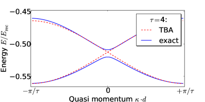
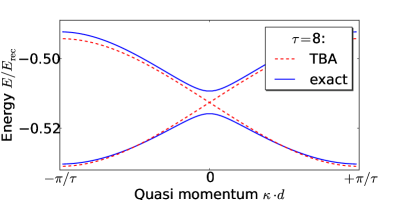
Figure 3: (Color online) Central energy bands for an optical superlattice $V_{\mathrm{sup}}$ [see Eq. (1)] with $V_{0}=2.42E_{\mathrm{rec}}$ and $V_{1}=0.06V_{0}$ for $\tau=4$ and $\tau=8$. In the tight-binding approximation (TBA—red dashed line) these energy bands touch whereas a gap is found in the exact calculation (exact—blue solid line).

Fourier-transformed states can be defined as

$$\Ket{\kappa,m}:=\sum_{l=0}^{\frac{N}{\tau}-1}\sqrt{\frac{\tau}{N}}e^{i\kappa\left(l\tau+\overline{m}\right)}\Ket{l,m},$$ (10)

where those $\Ket{\kappa,m}$ with $\kappa=\frac{2\pi}{N}s$, $s\in\mathbb{Z}$, $\kappa\in\left[-\frac{\pi}{\tau},\frac{\pi}{\tau}\right)$ form an orthonormal basis of the Hilbert subspace known as first Brillouin zone (1. BZ). Then, the bosonic (fermionic) annihilators and creators of those Fourier-transformed states are given by

$$\hat{b}_{m}(\kappa)=\sum_{l=0}^{\frac{N}{\tau}-1}\sqrt{\frac{\tau}{N}}e^{-i\kappa\left(l\tau+\overline{m}\right)}\hat{a}_{m}(l)$$ (11)

and its adjoint equation. They fulfill bosonic (fermionic) (anti-)commutator relations respectively. Introducing them into the Hamiltonian (Eq. (9)) and rewriting $\alpha=\overline{m+\Delta m}$, $\beta=\overline{m}$ gives

$$\hat{H} = \sum_{\kappa\in\textbf{1.BZ}}\sum_{\alpha,\beta=0}^{\tau-1}\sum_{\Delta l=0}^{\frac{N}{\tau}-1}\mathcal{J}\left((l+\Delta l)\tau+\alpha,l\tau+\beta\right)\times$$ (12)

$$\times e^{-i\kappa\left(\Delta l\tau+\alpha-\beta\right)}\hat{b}^{\dagger}_{\alpha}(\kappa)\hat{b}_{\beta}(\kappa)$$

$$= \sum_{\kappa\in\textbf{1.BZ}}\sum_{\alpha,\beta=0}^{\tau-1}\hat{b}^{\dagger}_{\alpha}(\kappa)\mathcal{M}_{\alpha\beta}\hat{b}_{\beta}(\kappa),$$

where the elements of the introduced matrix $\mathcal{M}$ can be calculated using Eq. (6) and performing the sum over $\Delta l$,

$$\mathcal{M}_{\alpha\beta} = \sum_{\Delta l=0}^{\frac{N}{\tau}-1}\mathcal{J}\left((l+\Delta l)\tau+\alpha,l\tau+\beta\right)e^{-i\kappa\left(\Delta l\tau+\alpha-\beta\right)}$$ (13)

$$= \frac{1}{\tau}\sum_{k}^{\kappa\star}e^{i(k-\kappa)\left(\alpha-\beta\right)}\Bigg{(}\epsilon(k)-V_{1}\frac{N}{\tau}\sum_{k^{\prime}}^{k\star}e^{i\beta\left(k-k^{\prime}\right)}\times$$

$$\times\int_{0}^{\tau}\textrm{d}y\cos\left(\frac{2\pi}{\tau}y\right)\Psi_{k}^{*}(y)\Psi_{k^{\prime}}(y)\Bigg{)}.$$

Here, $\sum_{k}^{q\star}$ denotes a sum over those quantum numbers $k\in[-\pi,\pi)$, which fulfill Eq. (2) and the condition $k-q=\frac{2\pi}{\tau}$, $s\in\mathbb{Z}$ for any value $q$. As can be shown, $\mathcal{M}$ is hermitian and thus, has real eigenvalues $E_{0}\ldots E_{\tau-1}$. The columns of the hermitian matrix $\mathcal{U}$, which diagonalizes $\mathcal{M}$, $\mathcal{U}\mathcal{M}\mathcal{U}^{\dagger}=\mathrm{diag}\left(E_{0},E_{1},\ldots,E_{\tau-1}\right)$, are given by the eigenvectors of $\mathcal{M}$. Finally, the creators and annihilators defined by

$$\left(\hat{\psi}^{\dagger}_{0}(\kappa),\ldots,\hat{\psi}^{\dagger}_{\tau-1}(\kappa)\right)=\left(\hat{b}^{\dagger}_{0}(\kappa),\ldots,\hat{b}^{\dagger}_{\tau-1}(\kappa)\right)\mathcal{U}^{\dagger}$$ (14)

and its adjoint eqution fulfill the bosonic (fermionic) (anti-)commutator relations respectively. Introducing them into Eq. (12) finally gives the diagonal Hamiltonian

$$\hat{H}=\sum_{\kappa\in\textbf{1.BZ}}\,\sum_{\alpha=0}^{\tau-1}E_{\alpha}(\kappa)\,\hat{\psi}_{\alpha}^{\dagger}(\kappa)\,\hat{\psi}_{\alpha}(\kappa).$$ (15)

Then, its $N$-particle bosonic or fermionic eigenstates are given in Fock space by

$$\Ket{n_{\alpha_{1}}(\kappa_{1}),\ldots,n_{\alpha_{N}}(\kappa_{N})}=\prod_{i=1}^{N}\frac{\left(\hat{\psi}_{\alpha_{i}}^{\dagger}(\kappa_{i})\right)^{n_{\alpha_{i}}(\kappa_{i})}}{\sqrt{n_{\alpha_{i}}(\kappa_{i})!}}\Ket{\emptyset}$$ (16)

for $\alpha_{i}\in[0,\tau-1]$, $\kappa_{i}\in\mathbf{1.BZ}$, and where $\Ket{\emptyset}$ denotes the vacuum state. The eigenenergies $E_{\alpha}(\kappa)$ are given by the eigenvalues of $\mathcal{M}$. They can be obtained easily, since the matrix elements $\mathcal{M}_{\alpha\beta}$ in Eq. (13) can be calculated analytically (see Supplemental Material).

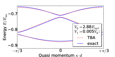
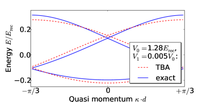
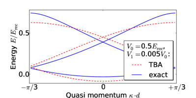
Figure 4: (Color online) Energy bands (TBA: red dashed, exact: blue solid) for an optical superlattice $V_{\mathrm{sup}}$ [see Eq. (1)] with periodicity $\tau=3$ for different values of the lattice depth $V_{0}$ (specified in the graphs) and the modulation $V_{1}=0.005V_{0}$.

Comparison to the TBA results — After the main result of this work, the exact diagonalization of the Hamiltonian, was presented, some implications are discussed. Whenever $\tau=4n$, $n$ being an integer, the TBA predicts the central energy bands to touch at $\kappa=0$ Rousseau et al. (2006). However, as can be seen from the exemplary cases $\tau=4$ and $\tau=8$ in Fig. 3, this contact disappears in the exact calculation. Therefore, the contact is an artifact of the TBA. As an important consequence, the in Rousseau et al. (2006) predicted non-insulating properties for superlattices with $\tau=4n$ and half filling of the states does not appear in reality. Besides this qualitative difference, there are, of course, also quantitative ones. As an example, Fig. 4 shows the energy bands for a $\tau=3$ superlattice with different depths $V_{0}$. Clearly, for deep lattices ($V_{0}\gtrsim 2.88$), a very good agreement between the TBA and the exact results is found, whereas for decreasing lattice depths ($V_{0}\lesssim 1.28$) the agreement becomes worse, as one would expect. Of course, only the exact results allow for a quantitative measure of the breakdown of the TBA. While for very weak modulation potentials $V_{1}$ ($V_{1}=0.005\,V_{0}$ in Fig. 4) the deviations of the TBA bands from the correct ones are relatively uniformly distributed over the quasi-momenta, this is not the case for larger modulation potentials. As can be seen in Fig. 5 ($V_{1}=0.5\,V_{0}$), the dispersion of the bands differs in a pronounced fashion between the TBA and the exact results. As a consequence, the gap is largely overestimated by the TBA. In fact, the TBA predicts almost discrete energy levels whereas the uppermost energy bands of the exact calculation are substantially broadened in the exemplary case $\tau=3$.

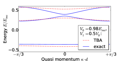
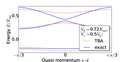
Figure 5: (Color online) as Fig. 4, but for $V_{0}=0.98\,E_{\mathrm{rec}}$ (top) and $V_{0}=0.72\,E_{\mathrm{rec}}$ (bottom) and a much stronger modulation potential $V_{1}=0.5V_{0}$.

Conclusion — As is shown in this work, the Hamiltonian of non-interacting particles in a general one-dimensional superlattice can be solved exactly without invoking the TBA as is done in the popular Hubbard models. The only assumption introduced is the restriction of the Hilbert space to the 1. Bloch band. In this case the problem can be reduced to the diagonalization of a square matrix with its dimension given by the periodicity $\tau$ of the superlattice and all matrix elements can be calculated exactly. Especially for periodicities $\tau=2$ or 3 fully analytical expressions can be found in principle and the solution includes the case of a uniform lattice ($V_{1}=0$). Thus, it is proven that the Schrödinger equation of non-interacting particles in a 1D superlattice, and thus of a problem that is of great interest in view of current experiments with ultracold atoms, belongs to the small class of exactly integrable quantum-mechanical problems. It is also possible to extend the indicated method to higher dimensions via a separation ansatz or to different translation-invariant lattice geometries such as graphene which has been studied within a tight-binding approximation in Semenoff (1984). Analogously to the other cases for which analytical solutions of the independent-particle problems (fully or within, e. g., the Hubbard model) exist, the present results can be the starting point for perturbative, numerical, or possibly even analytical solutions for the corresponding problem of interacting particles. Of course, as is demonstrated explicitly in this work, the exact solutions are useful for qualitatively and quantitatively determining the validity or failure of the popular tight-binding approximation.

References

- Greiner et al. (2002) M. Greiner, O. Mandel, T. Esslinger, T. Hänsch, and I. Bloch, Nature 415, 39 (2002).
- Lewenstein et al. (2007) M. Lewenstein, A. Sanpera, V. Ahufinger, B. Damski, A. Sen(De), and U. Sen, Adv. in Phys. 56, 243 (2007).
- Bloch et al. (2008) I. Bloch, J. Dalibard, and W. Zwerger, Rev. Mod. Phys. 80, 885 (2008).
- Jaksch et al. (1999) D. Jaksch, H.-J. Briegel, J. I. Cirac, C. W. Gardiner, and P. Zoller, Phys. Rev. Lett. 82, 1975 (1999).
- Jaksch et al. (1998) D. Jaksch, C. Bruder, J. I. Cirac, C. W. Gardiner, and P. Zoller, Phys. Rev. Lett. 81, 3108 (1998).
- Sebby-Strabley et al. (2006) J. Sebby-Strabley, M. Anderlini, P. S. Jessen, and J. V. Porto, Phys. Rev. A 73, 033605 (2006).
- Fölling et al. (2007) S. Fölling, S. Trotzky, P. Cheinet, M. Feld, R. Saers, A. Widera, T. Müller, and I. Bloch, Nature 448, 1029 (2007).
- Anderlini et al. (2006) M. Anderlini, J. Sebby-Strabley, J. Kruse, J. V. Porto, and W. D. Phillips, J. Phys. B 39, S199 (2006).
- Mazza et al. (2012) L. Mazza, A. Bermudez, N. Goldmann, M. Rizzi, M. A. Martin-Delgado, and M. Lewenstein, New J. Phys. 14, 015007 (2012).
- Bloch et al. (2012) I. Bloch, J. Dalibard, and S. Nascimbène, Nature Physics 8, 267 (2012).
- Rousseau et al. (2006) V. G. Rousseau, D. P. Arovas, M. Rigol, F. Hébert, G. G. Batrouni, and R. T. Scalettar, Phys. Rev. B 73, 174516 (2006).
- Chin et al. (2010) C. Chin, R. Grimm, P. Julienne, and E. Tiesinga, Rev. Mod. Phys. 82, 1225 (2010).
- Valiente et al. (2010) M. Valiente, M. Küster, and A. Saenz, EPL 92, 10001 (2010).
- Mattis (1993) D. C. Mattis, The Many-Body Problem – An Encyclopedia of Exactly Solvable Models in One Dimension (World Scientific Publishing, 1993).
- Cazalilla et al. (2011) M. A. Cazalilla, R. Cirto, T. Giamarchi, E. Orignac, and M. Rigol, Rev. Mod. Phys. 83, 1405 (2011).
- Hill (1886) G. W. Hill, Acta Math. 8, 1 (1886).
- Olver et al. (2010) F. W. J. Olver, D. W. Lozier, R. F. Boisvert, and C. W. Clark, eds., NIST Handbook of Mathematical Functions (Cambridge University Press, 2010).
- Semenoff (1984) G. W. Semenoff, Phys. Rev. Lett. 53, 2449 (1984).