Lengths of Monotone Subsequences in a Mallows Permutation

Abstract

We study the length of the longest increasing and longest decreasing subsequences of random permutations drawn from the Mallows measure. Under this measure, the probability of a permutation $\pi\in S_{n}$ is proportional to $q^{\operatorname{Inv}(\pi)}$ where $q$ is a real parameter and $\operatorname{Inv}(\pi)$ is the number of inversions in $\pi$. The case $q=1$ corresponds to uniformly random permutations. The Mallows measure was introduced by Mallows in connection with ranking problems in statistics.

We determine the typical order of magnitude of the lengths of the longest increasing and decreasing subsequences, as well as large deviation bounds for them. We also provide a simple bound on the variance of these lengths, and prove a law of large numbers for the length of the longest increasing subsequence. Assuming without loss of generality that $q<1$, our results apply when $q$ is a function of $n$ satisfying $n(1-q)\to\infty$. The case that $n(1-q)=O(1)$ was considered previously by Mueller and Starr. In our parameter range, the typical length of the longest increasing subsequence is of order $n\sqrt{1-q}$, whereas the typical length of the longest decreasing subsequence has four possible behaviors according to the precise dependence of $n$ and $q$.

We show also that in the graphical representation of a Mallows-distributed permutation, most points are found in a symmetric strip around the diagonal whose width is of order $1/(1-q)$. This suggests a connection between the longest increasing subsequence in the Mallows model and the model of last passage percolation in a strip.

1 Introduction

The length of the longest increasing subsequence of a uniformly random permutation has attracted the attention of researchers from several areas with significant contributions from Hammersley [19], Logan and Shepp [22] Vershik and Kerov [32], Aldous and Diaconis [1] and culminating with the breakthrough work of Baik, Deift and Johansson [4] who related this length to the theory of random matrices and proved that it has a Tracy-Widom limiting distribution. In this work we study the lengths of monotone subsequences (increasing or decreasing) of a random permutation having a different probability law, introduced by Mallows in [23] in order to study the statistical properties of non-uniformly random permutations (see also [13] and references therein for more background). The Mallows distribution is parameterized by a number $q>0$, with the probability of a permutation $\pi$ proportional to $q^{\operatorname{Inv}(\pi)}$, where $\operatorname{Inv}(\pi)$ is the number of inversions in $\pi$, or pairs of elements of $\pi$ which are out of order.

For $q>0$ and integer $n\geq 1$, the $(n,q)$-Mallows measure over permutations in $S_{n}$ is given by

$$\mu_{n,q}(\pi):=\frac{q^{\operatorname{Inv}(\pi)}}{Z_{n,q}},$$ (1)

where

$$\operatorname{Inv}(\pi):=|\{(i,j)\,:\,\text{$i<j$ and $\pi(i)>\pi(j)$}\}|$$

denotes the number of inversions in $\pi$, and $Z_{n,q}$ is a normalizing constant, given explicitly by the following well-known formula [27, pg. 21] (see also the remark after Lemma 2.1 below)

$$Z_{n,q}=\displaystyle\prod_{i=1}^{n}\frac{1-q^{i}}{1-q}.$$ (2)

Let $I=(i_{1},\ldots,i_{m})$ be an increasing sequence of indices. We say $I$ is an increasing subsequence of a permutation $\pi$ if $\pi(i_{k+1})>\pi(i_{k})$ for $1\leq k\leq m-1$. Define a decreasing subsequence analogously. Denote by $\operatorname{LIS}(\pi)$ the maximal length of an increasing subsequence in $\pi$. That is,

$$\operatorname{LIS}(\pi)=\max\{m\,:\,\exists\,i_{1}<\cdots<i_{m}\text{ satisfying }\pi(i_{1})<\cdots<\pi(i_{m})\}.$$

Analogously define $\operatorname{LDS}(\pi)$ to be the maximal length of a decreasing subsequence in $\pi$. That is,

$$\operatorname{LDS}(\pi)=\max\{m\,:\,\exists\,i_{1}<\cdots<i_{m}\text{ satisfying }\pi(i_{1})>\cdots>\pi(i_{m})\}.$$

Our goal is to investigate the distribution of $\operatorname{LIS}(\pi)$ and $\operatorname{LDS}(\pi)$ when $\pi$ is randomly sampled from the Mallows measure. We mention that the asymptotics of these lengths for other non-uniform distributions have been considered in the literature previously. For instance, Baik and Rains [5] study the longest increasing and decreasing subsequences of random permutations satisfying certain symmetry conditions such as uniformly chosen involutions. Féray and Méliot [15] studied a distribution similar to (1), but with $\operatorname{Inv}$ replaced by another permutation statistic, the major index. Fulman [16] relates the longest increasing subsequence in this major index distribution to the study of eigenvalues of random matrices over finite fields, analogously to the relation of the longest increasing subsequence of a uniform permutation with random Hermitian matrices. In addition, $\operatorname{LIS}(\pi)$ and $\operatorname{LDS}(\pi)$ have been studied for the Mallows distribution itself, by Mueller and Starr [24], as detailed below.

We focus our investigations on the Mallows measure with $q<1$. This restriction can be made without loss of generality since there is a duality between the measures $\mu_{n,q}$ and $\mu_{n,1/q}$. Indeed, if $\pi\sim\mu_{n,q}$ then its reversal $\pi^{R}$, defined by $\pi^{R}(i):=\pi(n+1-i)$, is distributed as $\mu_{n,1/q}$ (see Lemma 2.2 below). In particular, $\operatorname{LIS}(\pi)$ is distributed as $\operatorname{LDS}(\pi^{R})$. It is natural to allow $q$ to be a function of $n$. Mueller and Starr [24] studied the regime where $n(1-q)$ tends to a finite limit $\beta$. They showed that $\operatorname{LIS}(\pi)/\sqrt{n}$ converges in probability to $\ell(\beta)$, where $\ell(\beta)$ is an explicitly given function of $\beta$ satisfying $\ell(0)=2$ (see Theorem 5.2 for the precise statement), thus extending the results of [1, 22, 32]. This implies an analogous result for $\operatorname{LDS}(\pi)$ by the above-mentioned duality. Thus, in this limiting sense, in the regime where $n(1-q)$ tends to a finite constant as $n$ tends to infinity, $\operatorname{LIS}(\pi)$ and $\operatorname{LDS}(\pi)$ have the same order of magnitude as for a uniformly random permutation, with a different leading constant. In this paper we complete this picture by considering the case that $n(1-q)$ tends to infinity with $n$. We find the typical order of magnitude of $\operatorname{LIS}(\pi)$ and $\operatorname{LDS}(\pi)$ (which now differ from the uniformly random case) and establish large deviation results for these lengths and a law of large numbers for $\operatorname{LIS}(\pi)$. We also prove a simple bound on the variance of $\operatorname{LIS}(\pi)$ and $\operatorname{LDS}(\pi)$.

Our first result concerns the displacement $|\pi(i)-i|$ of an element in a random Mallows permutation. The result gives bounds on the tails of this displacement. This theorem is not used later in our analysis of monotone subsequences of random Mallows permutations but it is useful in developing intuition for their behavior. The upper bound follows by methods of Braverman and Mossel [8, Lemma 17] as well as Gnedin and Olshanski [18, Remark 5.2]. In [18], the authors studied a model of random permutations of the infinite group of integers $\mathbb{Z}$ which is obtained as a limit of the Mallows model, and obtained precise formulas for the distribution of displacements in this limiting model.

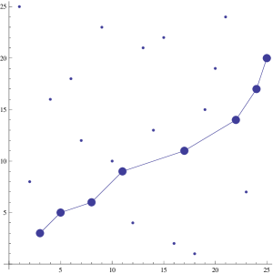
Figure 1: An increasing piecewise linear curve corresponding to a longest increasing subsequence.

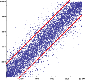
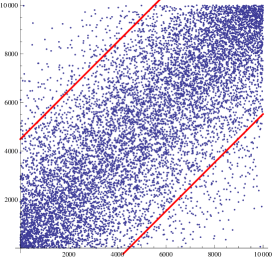
Figure 2: Graphical representation for random Mallows-distributed permutations with $1-q=n^{-0.7},\ n^{-0.8}$ and $n^{-0.88}$. The diagonal lines delineate a symmetric strip with width proportional to $\frac{1}{1-q}$. Theorem 1.1 shows that most points of the permutation must lie in such a strip.

Theorem 1.1.

For all $0<q<1$, and integer $n\geq 1$, $1\leq i\leq n$ and $t\geq 1$, if $\pi\sim\mu_{n,q}$ then

$$\mathbb{P}(|\pi(i)-i|\geq t)\leq 2q^{t},$$ (3)

and

$$c\min\left(\frac{q}{1-q},n-1\right)\leq\mathbb{E}|\pi(i)-i|\leq\min\left(\frac{2q}{1-q},n-1\right)$$ (4)

for some absolute constant $c>0$. In addition, if $n\geq 3$ and $1\leq t\leq\frac{n+5}{8}$ then

$$\mathbb{P}(|\pi(i)-i|\geq t)\geq\frac{1}{2}q^{2t-1}.$$

A permutation $\pi$ in $S_{n}$ can be naturally associated to a collection of $n$ points in the square $[1,n]^{2}$ by placing a point at $(i,\pi(i))$ for each $i$. In this graphical representation, increasing subsequences correspond to increasing curves passing through the points (see Figure 1), and decreasing subsequences correspond to decreasing curves. The graphical representation is depicted in Figure 2 for permutations simulated from the Mallows distribution $\mu_{n,q}$ for various choices of $n$ and $q$. The figure illustrates the fact that most points of the permutation are displaced by less than a constant times $q/(1-q)$, as Theorem 1.1 proves.

The previous remark suggests a connection between the study of the longest increasing subsequence of a random Mallows permutation, and the last passage percolation model in a strip. In one version of the latter model, one puts independent and identically distributed random points in a strip, and studies the last passage time, which is the same as the longest increasing subsequence when these points are taken to be the graphical representation of a permutation. In Section 8 we mention some works related to the limiting distribution of the last passage time and raise the question of whether the same limiting distributions arise also for the Mallows model.

Our next results concern the typical order of magnitude of $\operatorname{LIS}(\pi)$ when $\pi$ is sampled from the Mallows distribution. A heuristic guess for this order of magnitude may be obtained from Figure 3. Suppose that $\beta/(1-q)$ and $n(1-q)/\beta$ are integers for some large constant $\beta>0$. Consider $n(1-q)/\beta$ disjoint squares of side length $\beta/(1-q)$ along the strip delineated in the figure, such that the bottom left corner of each square equals the top right corner of the preceding square. The figure hints that the distribution of points in each square is close to a sample from the $\mu_{\beta/(1-q),q}$ distribution (here “close” should be interpreted as saying that the box contains a significant subsample of a Mallows distributed permutation of size $\beta/(1-q)$. Theorem 1.1 and the results in Section 2.1 give rigorous meaning to such statements). Thus the parameters fall in the regime of [24] and according to their results, the typical length of the longest increasing subsequence in each square is of order $1/\sqrt{1-q}$. We may thus create an increasing subsequence with length of order $n\sqrt{1-q}$ by concatenating the longest increasing subsequences in each of the $n(1-q)/\beta$ squares. This reasoning gives rise to the prediction that $\operatorname{LIS}(\pi)$ is about $Cn\sqrt{1-q}$ for some constant $C>0$. The next theorem establishes the correctness of this prediction, with a precise constant $C=1$, in the limit (5).

Theorem 1.2.

Let $(q_{n})$ be a sequence satisfying

$$q_{n}\to 1\quad\text{and}\quad n(1-q_{n})\to\infty$$ (5)

as $n$ tends to infinity. Suppose $\pi_{n}\sim\mu_{n,q_{n}}$. Then

$$\frac{\operatorname{LIS}(\pi_{n})}{n\sqrt{1-q_{n}}}\to 1$$

as $n$ tends to infinity, where the convergence takes place in $L_{p}$ for any $0<p<\infty$.

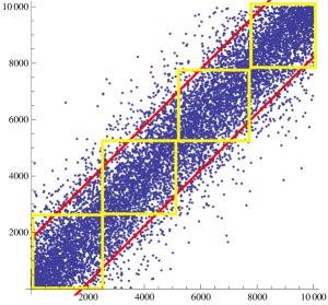
Figure 3: Disjoint boxes with side length $\frac{\beta}{1-q}$ along a symmetric strip around the diagonal.

In addition to this limiting behavior, Theorem 1.3 below gives large deviation bounds on the length of the longest increasing subsequence for fixed values of $n$ and $q$. The proof of Theorem 1.2 proceeds along the lines of the heuristic outlined above, combining our large deviation results with the weak law of large numbers shown in [24].

Notation: We will write $a_{n,q}\approx b_{n,q}$ if there exist absolute constants $0<c\leq C<\infty$ such that $cb_{n,q}\leq a_{n,q}\leq Cb_{n,q}$ for all $n$ and $q$ in a specified regime.

Theorem 1.3.

Suppose that $n\geq 1$, $\frac{1}{2}\leq q\leq 1-\frac{4}{n}$ and $\pi\sim\mu_{n,q}$. Then,

$$\mathbb{E}(\operatorname{LIS}(\pi))\approx n\sqrt{1-q}.$$ (6)

Furthermore, there exist absolute constants $0<C,c<\infty$ such that

1. For integer $L\geq Cn\sqrt{1-q}$,

   $$\left(\frac{c(1-q)n^{2}}{L^{2}}\right)^{L}\leq\mathbb{P}(\operatorname{LIS}(\pi)\geq L)\leq\left(\frac{C(1-q)n^{2}}{L^{2}}\right)^{L}.$$ (7)

2. For integer $n(1-q)\leq L\leq cn\sqrt{1-q}$,

   $$\mathbb{P}(\operatorname{LIS}(\pi)<L)\leq\exp\left(-\frac{c(1-q)n^{2}}{L}\right).$$ (8)

The bound (8) can be improved for certain regimes of $n,q$ and $L$; for details see section 6.3. Complementing the regime of $q$ in (6), we have the following simple bound on $\mathbb{E}(\operatorname{LIS}(\pi))$, which is rather precise for small $q$.

Proposition 1.4.

Suppose that $n\geq 1$, $0<q\leq 1$ and $\pi\sim\mu_{n,q}$. Then

$$n(1-q)\leq\mathbb{E}(\operatorname{LIS}(\pi))\leq n-\frac{q}{1+q}(n-1).$$

When $\pi$ is sampled uniformly from $S_{n}$, symmetry implies that $\operatorname{LIS}(\pi)$ and $\operatorname{LDS}(\pi)$ have the same distribution. For the Mallows measure, the analogous fact is not true. Indeed, looking at Figure 2 one expects $\operatorname{LDS}(\pi)$ to be of a smaller order of magnitude than $\operatorname{LIS}(\pi)$ when $\pi\sim\mu_{n,q}$ with $q<1$ since the overall trend of the points is positive. Our next theorem establishes the order of magnitude for $\operatorname{LDS}(\pi)$, confirming this expectation. Interestingly, we find as many as four different behaviors for this order of magnitude according to the relation between $n$ and $q$.

Theorem 1.5.

There exist constants $C_{0},c_{1}>0$ such that the following is true. Suppose that $n\geq 2$, $0<q<1$ and $\pi\sim\mu_{n,q}$.

1. $$\mathbb{E}(\operatorname{LDS}(\pi))\approx\begin{cases}\frac{1}{\sqrt{1-q}}&1-\frac{C_{0}}{(\log n)^{2}}\leq q\leq 1-\frac{4}{n}\\[10.00002pt] \frac{\log n}{\log((1-q)(\log n)^{2})}&1-\frac{c_{1}(\log\log n)^{2}}{\log n}\leq q\leq 1-\frac{C_{0}}{(\log n)^{2}}\\[10.00002pt] \sqrt{\frac{\log n}{\log\left(\frac{1}{q}\right)}}&\frac{1}{n}\leq q\leq 1-\frac{c_{1}(\log\log n)^{2}}{\log n}\end{cases}.$$ (9)

2. If $0<q\leq\frac{1}{n}$ then

   $$\mathbb{E}(\operatorname{LDS}(\pi))-1\approx nq.$$

We pause briefly to give an informal reasoning for the results of Theorem 1.5. As explained before Theorem 1.2 above, one may again employ the idea of placing $n(1-q)/\beta$ disjoint squares of side length $\beta/(1-q)$ along the diagonal as in Figure 3. Since we expect the distribution of the points in each such square to be close to that of the Mallows $\mu_{\beta/(1-q),q}$ measure, the results of [24] suggest that the typical order of magnitude of the length of the longest decreasing subsequence in each square is of order $1/\sqrt{1-q}$. When considering decreasing subsequences we cannot concatenate the subsequences of disjoint squares, since the overall trend of the points is positive. This heuristic suggests that $\operatorname{LDS}(\pi)$ should have order of magnitude at least as large as $1/\sqrt{1-q}$ and possibly not much larger. This is indeed the order of magnitude obtained in the first regime of Theorem 1.5. However, as $q$ decreases a different behavior takes over. Since we have $n(1-q)/\beta$ disjoint squares in which to consider the longest decreasing subsequence, we may expect that one of these squares exhibits atypical behavior, with a decreasing subsequence of order which is significantly longer than $1/\sqrt{1-q}$. The length of such an atypical decreasing subsequence may be predicted rather accurately using the large deviation results in Theorem 1.7 below and it turns out to be indeed significantly longer than $1/\sqrt{1-q}$ when $(\log n)^{2}(1-q)\to\infty$. This is what causes the transition between the first two regimes in Theorem 1.5. A different strategy for obtaining a decreasing subsequence should also be considered. Consider the length of a longest decreasing subsequence composed solely of consecutive elements, i.e., the largest $m$ for which $\pi(j)>\pi(j+1)>\ldots>\pi(j+m-1)$ for some $j$. The proof of Theorem 1.5 shows that the length of such a decreasing subsequence will have the same order of magnitude as the longest decreasing subsequence when $q$ is so small that the typical longest decreasing subsequence is longer than $1/(1-q)$. This is what governs the behavior in the third regime of the parameters in the theorem as well as in part of the second regime. Lastly, when $q\leq\frac{1}{n}$, i.e., in the fourth regime of the theorem, the probability that the random permutation differs from the identity is of order $nq$ (see Proposition 1.9 below). This is what governs the behavior in the fourth regime of the theorem.

Remark 1.6.

It seems likely that $\operatorname{LDS}(\pi)$ satisfies a law of large numbers similar to the one in Theorem 1.2. Indeed, if one formally takes the limit $\beta\to-\infty$ in the results of [24] one obtains that $\operatorname{LDS}(\pi)\sqrt{1-q}$ should tend to the constant $\pi$. We expect this result to hold when $n(1-q)\to\infty$ and $(\log n)^{2}(1-q)\to 0$, corresponding to the first regime in (9), see also Section 8.

Analogously to Theorem 1.3, we obtain large deviation estimates for $\operatorname{LDS}(\pi)$ holding for fixed $n$ and $q$.

Theorem 1.7.

There exist constants $C,c>0$ such that the following is true. Let $n\geq 2$, $0<q<1$ and $\pi\sim\mu_{n,q}$.

1. If $0<q<1-\frac{2}{n}$ then for integer $L\geq 2$,

   $$\mathbb{P}(\operatorname{LDS}(\pi)\geq L)\leq n^{8}\begin{cases}\left(\frac{C}{(1-q)L^{2}}\right)^{L}&L\leq\frac{3}{1-q}\\ (C(1-q))^{L}q^{\frac{L(L-1)}{2}}&L>\frac{3}{1-q}\end{cases}.$$ (10)

   Moreover, if $\;0<q<\frac{1}{2}$ then for integer $L\geq 2$,

   $$\mathbb{P}(\operatorname{LDS}(\pi)\geq L)\leq nC^{L}q^{\frac{L(L-1)}{2}}.$$ (11)

2. For integer $L$,

   $$\mathbb{P}(\operatorname{LDS}(\pi)\geq L)\geq\begin{cases}1-\left(1-\left(\frac{c}{(1-q)L^{2}}\right)^{L}\right)^{\lfloor\frac{n(1-q)}{4}\rfloor}&\text{if }\frac{C}{\sqrt{1-q}}\leq L\leq\frac{1}{1-q}\;\;\text{ and }\;\;\frac{1}{2}\leq q\leq 1-\frac{4}{n}\\ 1-\left(1-q^{\frac{L(L-1)}{2}}(1-q)^{L}\right)^{\lfloor\frac{n}{L}\rfloor}&\text{for any $L\geq 2$}\end{cases}.$$ (12)

3. Let $\frac{1}{2}\leq q\leq 1-\frac{4}{n}$. For integer $2\leq L<\frac{c}{\sqrt{1-q}}$,

   $$\mathbb{P}(\operatorname{LDS}(\pi)<L)\leq(C(1-q)L^{2})^{\frac{n}{L}}.$$ (13)

The discussion above focused on the typical order of magnitude and large deviations of $\operatorname{LIS}(\pi)$ and $\operatorname{LDS}(\pi)$ when $\pi$ is distributed according to the Mallows distribution. Also interesting, and seemingly more difficult, is the study of the typical deviations of $\operatorname{LIS}(\pi)$ and $\operatorname{LDS}(\pi)$ from their expected value. In this paper we make only a modest contribution towards understanding these quantities, as given in the following proposition. We denote by $\operatorname{Var}(X)$ the variance of $X$.

Proposition 1.8.

Let $n\geq 1,0<q<\infty$ and $\pi\sim\mu_{n,q}$. Then

$$\operatorname{Var}(\operatorname{LIS}(\pi))\leq n-1.$$

Furthermore, for all $t>0$,

$$\mathbb{P}(|\operatorname{LIS}(\pi)-\mathbb{E}(\operatorname{LIS}(\pi))|>t\sqrt{n-1})<2e^{-t^{2}/2}.$$

We note that the proposition applies equally well to the distribution of $\operatorname{LDS}(\pi)$ since it applies to arbitrary $q$ and, as noted above, the reversal of $\pi$ is distributed as $\mu_{n,1/q}$, and satisfies that $\operatorname{LIS}(\pi)=\operatorname{LDS}(\pi^{R})$. We expect that when $n$ tends to infinity with $0<q<1$ fixed then $\operatorname{Var}(\operatorname{LIS}(\pi))$ will indeed be of order $n$. However, if $q$ increases to $1$ as $n$ tends to infinity then we expect the variance to be of smaller order, see the discussion in Section 8.

We finish the description of our main results with a simple proposition which is useful for very small $q$. It shows that when $nq$ is much smaller than $1$, the Mallows distribution is concentrated on the identity permutation.

Proposition 1.9.

Suppose $n\geq 2$, $0<q\leq\frac{1}{n}$ and $\pi\sim\mu_{n,q}$. Then

$$\mathbb{P}(\pi\text{ is not the identity})\approx nq.$$

Policy on constants: In what follows, $C$ and $c$ denote positive numerical constants (independent of all other parameters) whose value can change each time they occur (even inside the same calculation), with the value of $C$ increasing and the value of $c$ decreasing. In contrast, the value of numbered constants, such as $C_{0}$ or $c_{0}$, is fixed and will not change between occurrences.

1.1 Techniques

Previous work on the asymptotics of the longest increasing subsequence followed two main approaches: either through analysis of combinatorial asymptotics or by the probabilistic analysis of systems of interacting particle processes. The combinatorial approach to the longest increasing subsequence makes use of a bijection between permutations and Young tableaux known as the Robinson-Schensted-Knuth (RSK) correspondence [25, 26, 21]. This bijection is intimately related to the representation theory of the symmetric group [20, 12], the theory of symmetric functions [28], and the theory of partitions [3]. The uniform measure on permutations induces the Plancherel measure on Young diagrams under the RSK correspondence. Vershik and Kerov and Logan and Shepp independently showed a limiting shape for diagrams under the Plancherel measure and proved that

$$\mathbb{E}(\operatorname{LIS}(\pi))=2\sqrt{n}+o(\sqrt{n})\quad\text{when $\pi$ is uniformly distributed}.$$ (14)

This approach was extended much later in the groundbreaking work of Baik, Deift and Johansson [4] who determined completely the limiting distribution and fluctuations of the longest increasing subsequence of a uniformly distributed permutation.

The second approach has been through the framework of interacting particle processes. Hammersley [19] investigated “Ulam’s problem” of finding the constant in the expected length of the longest monotone subsequence in a uniformly random permutation. Implicit in this work was a certain one-dimensional interacting particle process which Aldous and Diaconis [1] call Hammersley’s process. Aldous and Diaconis gave hydrodynamical limiting arguments for Hammersley’s process to obtain an independent proof of the result (14). This approach led to other generalizations, such as the work of Deuschel and Zeitouni [10] who found the leading behavior of $\mathbb{E}(\operatorname{LIS}(\pi))$ when $\pi$ is a random permutation whose graphical representation is obtained by putting independent and identically distributed points in the plane.

Mueller and Starr [24] were the first to consider the longest increasing subsequence of a random Mallows permutation. Their work focuses on the regime of parameters where $n(1-q)\to\beta\in(-\infty,\infty)$ as $n\to\infty$. In this regime Starr [29] developed a Botzmann-Gibbs formulation of the Mallows measure and found a limiting density for the graphical representation of the random permutation. Mueller and Starr relied on this limiting density and applied similar techniques to those of Deuschel and Zeitouni [10] to find the leading behavior of $\mathbb{E}(\operatorname{LIS}(\pi))$.

Our analysis uses a third approach. In his paper, Mallows [23] describes an iterative procedure for generating a Mallows-distributed permutation. This procedure, which we term the Mallows process, is defined formally in Section 2. Informally, it may be described as follows: A set of $n$ folders is put in a random order into a drawer using the rule that each new folder is inserted at a random position, pushing back all the folders behind it. The probability that the $i$th folder is inserted at position $j$, for $1\leq j\leq i$, is proportional to $q^{j-1}$, independently of all other folders. It is not hard to check that after all $n$ folders have been placed in the drawer, their positions have the $(n,1/q)$-Mallows distribution. Our analysis consists of tracking the dynamics of the increasing and decreasing subsequences throughout the evolution of this process.

1.2 Reader’s guide

The remainder of the paper is organized as follows. In Section 2 we define the Mallows process formally and derive some useful properties of the Mallows measure from it. In Section 3 we bound the displacement of elements in a random Mallows permutation, proving Theorem 1.1. Section 4 is devoted to the study of $\operatorname{LIS}(\pi)$. We establish there the large deviation bounds for $\operatorname{LIS}(\pi)$ and determine its typical order of magnitude, proving Theorem 1.3 and Proposition 1.4. In Section 5 we prove the law of large numbers for $\operatorname{LIS}(\pi)$, establishing Theorem 1.2. In Section 6 we study $\operatorname{LDS}(\pi)$, establishing large deviation bounds for it and determining its typical order of magnitude, proving Theorem 1.5, Theorem 1.7 and Proposition 1.9. In Section 7 we prove Proposition 1.8, giving a simple bound on the variance of $\operatorname{LIS}(\pi)$ and showing a Gaussian tail inequality. Finally, we end with some directions for further research in Section 8.

1.3 Acknowledgements

We thank Elchanan Mossel for pointing out to us that the technique of proof in [8, Lemma 17] simplifies our previous proof of the upper bound in (4) and yields also the deviation bound (3).

2 The Mallows process

In this section we describe a random evolution process on permutations, which we term the Mallows process. This process is central to our later analysis of the length of monotone subsequences. The process was known to Mallows [23], and was also used by Gnedin and Olshanski [17, 18] to study variants and extensions of the Mallows measure to infinite groups of permutations. The underlying idea is also useful in the analysis of the number of inversions of a uniformly random permutation, e.g., as in Feller [14, Chap. X.6].

Let $q>0$. The $q$-Mallows process is a permutation-valued stochastic process $(p_{n})_{n\geq 1}$, where each $p_{n}\in S_{n}$. The process is initialized by setting $p_{1}$ to be the (only) permutation on one element. The process iteratively constructs $p_{n}$ from $p_{n-1}$ and an independent random variable $p_{n}(n)$ distributed as a truncated geometric. Precisely, letting $(p_{n}(n))$ be a sequence of independent random variables with the distributions

$$\mathbb{P}(p_{n}(n)=j):=\frac{q^{j-1}}{1+q+\cdots+q^{n-1}}=\frac{(1-q)q^{j-1}}{1-q^{n}}\quad(1\leq j\leq n),$$ (15)

each permutation $p_{n}$ is defined by

$$p_{n}(i)=\begin{cases}p_{n-1}(i)&p_{n-1}(i)<p_{n}(n)\\ p_{n-1}(i)+1&p_{n-1}(i)\geq p_{n}(n)\end{cases}\quad(1\leq i\leq n-1).$$ (16)

Alluding to our intuitive description in Section 1.1, we may think of $p_{n}(i)$ as denoting the position of the $i$th folder at time $n$ in the drawer. It is clear by construction that $p_{n}$ is a permutation in $S_{n}$. Also, note that for each $i$ and $n\geq i$, $p_{n}(i)$ is non-decreasing in $n$. Below is an example to illustrate the process. For example, we see that in the second step $n=2$, since the position of the second folder is $1$, the position of the first folder becomes $2$. In general, in step $n$, the position of a folder increases by $1$ if its position in step $n-1$ is at or after the position where the $n$th folder is inserted and otherwise it stays the same. We also note the process $(p_{n}^{-1})$ which may be thought of as the contents of the drawer at time $n$, in the intuitive description of Section 1.1.

$$\begin{array}[]{ccll}n&p_{n}(n)&p_{n}&(p_{n}^{-1})\\ 1&1&1&1\\ 2&1&21&21\\ 3&2&312&231\\ 4&4&3124&2314\\ 5&2&41352&25314\\ 6&3&514623&256314\\ \end{array}$$

Lemma 2.1.

Let $q>0$ and let $(p_{n})_{n\geq 1}$ be the $q$-Mallows process. Then $p_{n}$ is distributed according to the Mallows distribution with parameter $1/q$.

Proof.

The claim is trivial for $n=1$. Assume by induction that for any $\sigma_{n}\in S_{n}$, $\mathbb{P}(p_{n}=\sigma_{n})\propto q^{-\operatorname{Inv}(\sigma_{n})}$ and let us prove the same for $n+1$. Fix a permutation $\sigma_{n+1}\in S_{n+1}$. For $1\leq i\leq n$, define a permutation $\sigma_{n}\in S_{n}$ by

$$\sigma_{n}(i):=\begin{cases}\sigma_{n+1}(i)-1&\text{ if }\sigma_{n+1}(i)>\sigma_{n+1}(n+1)\\ \sigma_{n+1}(i)&\text{ if }\sigma_{n+1}(i)<\sigma_{n+1}(n+1)\\ \end{cases}$$

It follows from the definition of the Mallows process that $p_{n+1}=\sigma_{n+1}$ if and only if $p_{n+1}(n+1)=\sigma_{n+1}(n+1)$ and $p_{n}=\sigma_{n}$. Noting that $\operatorname{Inv}(\sigma_{n+1})=\operatorname{Inv}(\sigma_{n})+n+1-\sigma_{n+1}(n+1)$, the induction hypothesis implies that

$$\mathbb{P}(p_{n+1}=\sigma_{n+1}) =\mathbb{P}(p_{n}=\sigma_{n})\cdot\mathbb{P}(p_{n+1}(n+1)=\sigma_{n+1}(n+1))$$

$$=\frac{q^{-\operatorname{Inv}(\sigma_{n})}}{Z_{n,1/q}}\cdot\frac{q^{\sigma_{n+1}(n+1)-1}}{1+q+\cdots+q^{n}}$$

$$=\frac{q^{-\operatorname{Inv}(\sigma_{n})}}{Z_{n,1/q}}\cdot\frac{(1/q)^{n-\sigma_{n+1}(n+1)+1}}{1+(1/q)+\cdots+(1/q)^{n}}\propto q^{-\operatorname{Inv}(\sigma_{n+1})}.\qed$$

As a by-product, the above recursion also shows that the formula (2) for the normalizing constant holds. Recall that $\pi^{R}$, the reversal of a permutation $\pi$, is defined by $\pi^{R}(i)=\pi(n+1-i)$.

Lemma 2.2.

For any $n\geq 1$ and $q>0$, if $\pi\sim\mu_{n,q}$ then $\pi^{R}\sim\mu_{n,1/q}$ and $\pi^{-1}\sim\mu_{n,q}$.

Proof.

The lemma is immediate upon noting that both taking reversal and taking inverse are bijections on $S_{n}$, and that $\operatorname{Inv}(\pi^{R})={n\choose 2}-\operatorname{Inv}(\pi)$ and $\operatorname{Inv}(\pi^{-1})=\operatorname{Inv}(\pi)$. ∎

This lemma allows us to define four different permutations related to the $q$-Mallows process, all having the Mallows distribution $\mu_{n,q}$.

Corollary 2.3.

Let $q>0$ and let $(p_{n})_{n\geq 1}$ be the $q$-Mallows process. Then each of the following permutations is distributed as $\mu_{n,q}$.

1. $\pi:=p_{n}^{R}$. That is, $\pi(i)=p_{n}(n+1-i)$.

2. $\pi:=(p_{n}^{R})^{-1}$. That is, $\pi(i)=n+1-p_{n}^{-1}(i)$.

3. $\pi:=(p_{n}^{-1})^{R}$. That is, $\pi(i)=p_{n}^{-1}(n+1-i)$.

4. $\pi:=((p_{n}^{-1})^{R})^{-1}$. That is, $\pi(i)=n+1-p_{n}(i)$.

This corollary will be useful in the sequel, allowing us to prove results about the Mallows distribution by choosing from the above list a convenient coupling of the Mallows distribution and the Mallows process.

2.1 Basic properties of the Mallows process

In this section we let $q$ be an arbitrary positive number and let $(p_{n})$ be the $q$-Mallows process. Let $I=(i_{1},\ldots,i_{k})$ be an increasing sequence of indices and let $\pi$ be any permutation. Let $\pi_{I}\in S_{k}$ denote the induced relative ordering of $\pi$ restricted to $I$. That is, $\pi_{I}(j)>\mathscr{\pi}_{I}(k)$ if and only if $\pi(i_{j})>\pi(i_{k})$. The following fact is clear from the definition of the Mallows process.

Fact 2.4.

Let $I=(i_{1},\ldots,i_{k})$ be an increasing sequence and let $n\geq i_{k}$. Then $(p_{n})_{I}$ is a function only of $p_{i_{1}}(i_{1}),p_{i_{1}+1}(i_{1}+1),\ldots,p_{i_{k}-1}(i_{k}-1),p_{i_{k}}(i_{k})$. In other words, $(p_{n})_{I}$ is independent of the set of $(p_{i})_{i}$, $i<i_{1}$ or $i>i_{k}$.

Lemma 2.5.

(Independence of induced orderings) Let $I=(i_{1},\ldots,i_{k})$ and $I^{\prime}=(i^{\prime}_{1},\ldots,i^{\prime}_{\ell})$ be two increasing sequences such that $i_{k}<i_{1}^{\prime}$. Let $\pi\sim\mu_{n,q}$ for $n\geq i^{\prime}_{\ell}$. Then, $\pi_{I}$ and $\pi_{I^{\prime}}$ are independent.

Proof.

Using Corollary 2.3, we couple $\pi$ with $(p_{n})$ so that $\pi(i)=n+1-p_{n}(i)$ for all $i$. By the definition of the Mallows process, the variables $(p_{i}(i))$ are independent. By Fact 2.4, $\pi_{I}$ and $\pi_{I^{\prime}}$ are functions of independent variables and are therefore independent. ∎

For a sequence of indices $I=(i_{1},\ldots,i_{m})$ and an integer $b$, define the sequence $I+b:=(i_{1}+b,\ldots,i_{m}+b)$.

Lemma 2.6.

(Translation invariance) Let $I=(i_{1},\ldots,i_{k})$ be an increasing sequence and let $\pi\sim\mu_{n,q}$. Then, for any integer $1\leq b\leq n-i_{k}$, $\pi_{I}$ and $\pi_{I+b}$ have the same distribution. That is, for any $\omega\in S_{k}$,

$$\mathbb{P}(\pi_{I}=\omega)=\mathbb{P}(\pi_{I+b}=\omega).$$

Proof.

Observe that we can make the following simplifying assumptions. First, we may assume that $b=1$ since then the claim follows by applying the result $b$ times. Second, under the assumption $b=1$, $I$ is contained in $(1,2,\ldots,n-1)$ and hence we may deduce the lemma with the given $I$ from the lemma with $I=(1,2,\ldots,n-1)$.

Assume then that $b=1$ and $I=(1,2,\ldots,n-1)$. It is straightforward to see that there exists a unique bijection $T$ from $S_{n}$ to itself which preserves the number of inversions (and hence the Mallows distribution), such that $(T(\pi))_{I+1}=\pi_{I}$. This establishes the lemma. ∎

It is simple to check that the above fact is not necessarily true for sequences which are not translates. Suppose $\pi\sim\mu_{3,q}$. By explicit calculation,

$$\mathbb{P}(\pi(2)>\pi(1))=\frac{1+q+q^{2}}{Z_{3,q}}\quad\text{whereas}\quad\mathbb{P}(\pi(3)>\pi(1))=\frac{1+2q}{Z_{3,q}},$$

so that the probabilities are different for all $q\neq 1$.

One corollary of translation invariance is that the permutation induced on any sequence of consecutive elements is distributed like a shorter Mallows permutation.

Corollary 2.7.

Let $I=(i,i+1,\ldots,i+m-1)\subseteq[n]$ be a sequence of consecutive elements. If $\pi\sim\mu_{n,q}$ then $\pi_{I}\sim\mu_{m,q}$.

Proof.

Since $q$ is arbitrary, it suffices to prove the corollary with $\pi$ replaced by $p_{n}$, so that $q$ is replaced by $1/q$. For $i=1$, the claim follows simply by the definition of the Mallows process. That is, since $\pi_{I}=p_{m}\sim\mu_{m,1/q}$. For $i>1$, the claim follows by the translation invariance given by Lemma 2.6. ∎

Remark 2.8.

One can also construct a Mallows permutation indexed by the infinite sets $\mathbb{N}$ or $\mathbb{Z}$ [17, 18]. A version of Corollary 2.7 would still be valid in this case, yielding the finite Mallows distribution as an induced permutation of the infinite one. The infinite permutation has the advantage that it is constructed out of a sequence of i.i.d. geometric random variables rather than just independent truncated geometric variables as in the finite construction. However, the fact that the geometric random variables are unbounded complicates some aspects of our proofs and in this paper we chose to work only in the finite setting.

3 The Displacement of an element in a Mallows permutation

In this section we prove Theorem 1.1. Our proof of the upper bounds follows that of [8, Lemma 17], with slightly more precise estimates.

Fix $0<q<1$. Recall the $q$-Mallows process $(p_{i})$ from Section 2, defined for all $i\geq 1$. We first prove the upper bounds in the theorem. Fix $n\geq 1$ and consider the permutation $\pi$ defined by $\pi(i):=n+1-p_{n}(i)$, which by Corollary 2.3 is distributed according to $\mu_{n,q}$. Note first that for all $1\leq i\leq n$,

$$\pi(i)-i=n+1-p_{n}(i)-i=n-i-p_{n}(i)+p_{i}(i)-(p_{i}(i)-1).$$

Thus, since $p_{i}(i)\geq 1$ and $p_{n}(i)-p_{i}(i)\leq n-i$, we have

$$|\pi(i)-i|{\mathbbm{1}}_{(\pi(i)-i<0)}\leq p_{i}(i)-1\quad\text{ for }1\leq i\leq n.$$ (17)

Similarly, let $\pi^{\prime}$ be defined by $\pi^{\prime}(i):=p_{n}(n+1-i)$, so that $\pi^{\prime}\sim\mu_{n,q}$ by Corollary 2.3. For all $1\leq i\leq n$,

$$\pi^{\prime}(n+1-i)-(n+1-i)=p_{n}(i)-(n+1-i)=-(n-i-p_{n}(i)+p_{i}(i))+(p_{i}(i)-1).$$

Thus, again since $p_{i}(i)\geq 1$ and $p_{n}(i)-p_{i}(i)\leq n-i$, we have

$$|\pi^{\prime}(n+1-i)-(n+1-i)|{\mathbbm{1}}_{(\pi^{\prime}(n+1-i)-(n+1-i)>0)}\leq p_{i}(i)-1,$$

and exchanging the roles of $i$ and $n+1-i$ we obtain

$$|\pi^{\prime}(i)-i|{\mathbbm{1}}_{(\pi^{\prime}(i)-i>0)}\leq p_{n+1-i}(n+1-i)-1\quad\text{ for }1\leq i\leq n.$$ (18)

Putting together (17) and (18), and recalling that $\pi,\pi^{\prime}\sim\mu_{n,q}$ we conclude that for all $1\leq i\leq n$ and integer $t\geq 1$,

$$\mathbb{P}(|\pi(i)-i|\geq t)=\mathbb{P}(\pi(i)-i\geq t)+\mathbb{P}(\pi(i)-i\leq-t)\leq\mathbb{P}(p_{n+1-i}(n+1-i)\geq t+1)+\mathbb{P}(p_{i}(i)\geq t+1).$$ (19)

Now recall from (15) that $p_{j}(j)$ has the distribution of a geometric random variable with parameter $1-q$, conditioned to be at most $j$. In particular, $p_{j}(j)$ is stochastically dominated by this geometric random variable and thus

$$\mathbb{P}(p_{j}(j)\geq t+1)\leq q^{t}\quad\text{ for }1\leq j\leq n\text{ and integer }t\geq 1.$$ (20)

Putting together (19) and (20) yields (3). Thus, the upper bound of (4) follows since $|\pi(i)-i|\leq n-1$ and

$$\mathbb{E}|\pi(i)-i|=\sum_{t=1}^{\infty}\mathbb{P}(|\pi(i)-i|\geq t)\leq\sum_{t=1}^{\infty}2q^{t}=\frac{2q}{1-q}.$$

Next we derive a lower bound on the displacement. This is done in the next three claims. We start by observing a monotonicity property of the Mallows process. Let

$$A=\{(a_{1},a_{2},\ldots)\,:\,a_{j}\in\{1,\ldots,j\}\}.$$

By definition of the Mallows process, for each $n$, the permutation $p_{n}$ is a function of the vector $(p_{1}(1),\ldots,p_{n}(n))$, whose elements satisfy $p_{j}(j)\in\{1,\ldots,j\}$. For $a\in A$, denote by $p_{n}^{a}$ the permutation $p_{n}$ resulting from taking $p_{j}(j)=a_{j}$.

Lemma 3.1.

For each $n\geq 1$ and $1\leq j\leq n$, $p_{n}^{a}(j)$ is increasing in $a_{j}$. That is, if $a,a^{\prime}\in A$ satisfy $a_{k}=a^{\prime}_{k}$ for all $k\neq j$ and $a_{j}>a^{\prime}_{j}$ then $p_{n}^{a}(j)>p_{n}^{a^{\prime}}(j)$.

Proof.

Fix $n,j,a,a^{\prime}$ as in the lemma. Trivially $p_{j}^{a}(j)>p_{j}^{a^{\prime}}(j)$. Hence it suffices to observe by induction that for $k\geq j$,

$$p_{k+1}^{a}(j)=p_{k}^{a}(j)+\mathbbm{1}_{(a_{k+1}\leq p_{k}^{a}(j))}=p_{k}^{a}(j)+\mathbbm{1}_{(a^{\prime}_{k+1}\leq p_{k}^{a}(j))}>p_{k}^{a^{\prime}}(j)+\mathbbm{1}_{(a^{\prime}_{k+1}\leq p_{k}^{a^{\prime}}(j))}=p_{k+1}^{a^{\prime}}(j).\qed$$

Lemma 3.2.

For all integer $n\geq 1,1\leq i\leq n$ and $t\geq 1$, if $\pi\sim\mu_{n,q}$ then

$$\mathbb{P}(|\pi(i)-i|\geq t)\geq\max(\mathbb{P}(p_{i}(i)\geq 2t),\,\mathbb{P}(p_{n+1-i}(n+1-i)\geq 2t)).$$

Proof.

Fix $n,i$ and $t$ as in the lemma. Couple $\pi$ with the Mallows process so that $\pi(j)=n+1-p_{n}(j)$ as in Corollary 2.3. Condition on $(p_{j}(j))$ for $j\neq i$ and observe that under this conditioning, the value of $p_{n}(i)$, and hence the value of $\pi(i)$, is a function of $p_{i}(i)$. By Lemma 3.1, under the conditioning, there are at most $2t-1$ (contiguous) values of $p_{i}(i)$ for which $|\pi(i)-i|<t$. Since the $(p_{j}(j))$ are independent and $\mathbb{P}(p_{i}(i)=s)$ is a decreasing function of $s$, it follows that

$$\mathbb{P}(|\pi(i)-i|\geq t)=\mathbb{E}\left[\mathbb{P}(|\pi(i)-i|\geq t\,|\,(p_{j}(j))_{j\neq i})\right]\geq\mathbb{E}\left[\mathbb{P}(p_{i}(i)\geq 2t\,|\,(p_{j}(j))_{j\neq i})\right]=\mathbb{P}(p_{i}(i)\geq 2t).$$

The proof of the bound $\mathbb{P}(|\pi(i)-i|\geq t)\geq\mathbb{P}(p_{n+1-i}(n+1-i)\geq 2t)$ is analogous by using the coupling $\pi(j)=p_{n}(n+1-j)$ of Corollary 2.3 and applying Lemma 3.1 with $j=n+1-i$. ∎

Corollary 3.3.

For all integer $n\geq 3,1\leq i\leq n$ and $1\leq t\leq\frac{n+5}{8}$, if $\pi\sim\mu_{n,q}$ then

$$\mathbb{P}(|\pi(i)-i|\geq t)\geq\frac{1}{2}q^{2t-1}.$$

Proof.

Let $j=\max(i,n+1-i)$. Observe that $j\geq\frac{n+1}{2}$. Note also that our assumptions imply that $2t\leq\frac{n+1}{2}\leq j$. By Lemma 3.2 and (15),

$$\mathbb{P}(|\pi(i)-i|\geq t)\geq\mathbb{P}(p_{j}(j)\geq 2t)=\frac{1-q^{j-2t+1}}{1-q^{j}}q^{2t-1}.$$

Our assumptions imply that $t\leq\frac{n+5}{8}\leq\frac{j+2}{4}$ and thus $j-2t+1\geq\frac{j}{2}$. Hence we conclude that

$$\mathbb{P}(|\pi(i)-i|\geq t)\geq\frac{1-q^{j/2}}{1-q^{j}}q^{2t-1}=\frac{q^{2t-1}}{1+q^{j/2}}\geq\frac{1}{2}q^{2t-1}.\qed$$

Finally, we fix $n\geq 2,1\leq i\leq n$ and prove a lower bound for $\mathbb{E}|\pi(i)-i|$. We consider separately three cases. If $n\geq 3$ and $q<1-\frac{1}{n}$ then by Corollary 3.3,

$$\mathbb{E}|\pi(i)-i|\geq\sum_{t=1}^{\lfloor\frac{n+5}{8}\rfloor}\mathbb{P}(|\pi(i)-i|\geq t)\geq\frac{1}{2}\sum_{t=1}^{\lfloor\frac{n+5}{8}\rfloor}q^{2t-1}=\frac{q(1-q^{2\lfloor(n+5)/8\rfloor})}{2(1-q^{2})}\geq c\frac{q}{1-q}$$

for some absolute constant $c>0$. If $n\geq 3$ and $q\geq 1-\frac{1}{n}$ then, similarly, by Corollary 3.3,

$$\mathbb{E}|\pi(i)-i|\geq\sum_{t=1}^{\lfloor\frac{n+5}{8}\rfloor}\mathbb{P}(|\pi(i)-i|\geq t)\geq\frac{1}{2}\sum_{t=1}^{\lfloor\frac{n+5}{8}\rfloor}q^{2t-1}\geq\frac{1}{2}\sum_{t=1}^{\lfloor\frac{n+5}{8}\rfloor}\left(1-\frac{1}{n}\right)^{2t-1}\geq cn$$

for some absolute constant $c>0$. Finally, if $n=2$ then by Lemma 3.2,

$$\mathbb{E}|\pi(i)-i|=\mathbb{P}(|\pi(i)-i|\geq 1)\geq\mathbb{P}(p_{2}(2)\geq 2)=\frac{q}{1+q}\geq\frac{q}{2}.$$

Thus in all cases we have shown that $\mathbb{E}|\pi(i)-i|\geq c\min\left(\frac{q}{1-q},n-1\right)$, as required.

4 Increasing subsequences

Our goal in this section is to establish Theorem 1.3 and Proposition 1.4. We begin in Section 4.1 with the lower bound in (7) and the bound (8). In Section 4.2 we use a union bound argument to show that the probability of a very long increasing subsequence cannot be too large and establish the upper bound in (7). In the same section we complete the proof of Theorem 1.3 and Proposition 1.4 by applying the previous results to estimate the expectation of $\operatorname{LIS}(\pi)$. Lastly, a result extending our tail bounds for $\operatorname{LIS}(\pi)$ is proved at the end of Section 4.2. This result is used in the arguments of Section 5.

4.1 Lower bounds on the probability of a long increasing subsequence

In this section we will show a lower bound on the probability that there is a long increasing subsequence, proving the lower bound of (7) and the bound (8) in Theorem 1.3. The proof proceeds by defining a sequence of stopping times for the Mallows process at which elements are added to an increasing subsequence. We show that the waiting time to build a long increasing subsequence in this way is not too large with high probability.

4.1.1 Large deviation bounds for binomial random variables

The next proposition collects some standard results on binomial random variables which will be used in the sequel.

Proposition 4.1.

Suppose $n\geq 1$, $0<p<1$ and let $S\sim\operatorname{Bin}(n,p)$.

1. For all $t>0$,

   $$\mathbb{P}(S-np<-t)<\exp\left(-\frac{t^{2}}{2np}\right).$$

   In particular,

   $$\mathbb{P}\left(S<\frac{1}{2}np\right)\leq\exp\left(-\frac{1}{8}np\right).$$ (21)

2. If $p<\frac{1}{2}$ then for all integer $np\leq t\leq n$,

   $$\mathbb{P}(S\geq t)\geq\left(\frac{np}{et}\right)^{t}.$$ (22)

Proof.

The first part is proved, for instance, in [2, Theorem A.1.13]. For the second part, observe first that

$$\mathbb{P}(S\geq t)\geq\binom{n}{t}p^{t}(1-p)^{n-t}\geq\left(\frac{np}{t}\right)^{t}(1-p)^{n-t}.$$

Now note that $\log(1-p)\geq-p-p^{2}$ for $0\leq p\leq 1/2$. Thus, using that $t\geq np$ in the third inequality,

$$\mathbb{P}(S\geq t)\geq\left(\frac{np}{t}\right)^{t}e^{-(n-t)(p+p^{2})}\geq\left(\frac{np}{t}\right)^{t}e^{-np+p(t-np)}\geq\left(\frac{np}{t}\right)^{t}e^{-t}.\qed$$

4.1.2 Lower bounds for $\mathbb{P}(\operatorname{LIS}(\pi)\geq L)$

Fix $n\geq 1$ and $\frac{1}{2}\leq q\leq 1-\frac{4}{n}$. Let $(p_{m})$ be the $q$-Mallows process, and define, for $m\geq 1$, $\pi_{m}:=(p_{m})^{R}$ so that $\pi_{m}\sim\mu_{m,q}$ by Corollary 2.3. Fix an integer $1\leq L\leq n$ and consider the following strategy for finding an increasing subsequence in $\pi_{n}$. Let

$$W:=\left[\frac{1}{1-q},\,\frac{1}{1-q}+\frac{n}{1000L}+1\right]\cap\mathbb{Z}$$

and set $T_{0}:=\max(W)$. Consider the minimal time $S_{1}>T_{0}$ for which $p_{S_{1}}(S_{1})\in W$, and consider the first subsequent time $T_{1}>S_{1}$ for which $p_{T_{1}}(S_{1})\notin W$. Then repeat the process and find the next subsequent time $S_{2}>T_{1}$ for which $p_{S_{2}}(S_{2})\in W$, and so on. Formally, with $T_{0}=\max(W)$, we inductively define the stopping times for $i\geq 1$ as follows:

$$S_{i} :=\min\{t>T_{i-1}\ :\ p_{t}(t)\in W\},$$

$$T_{i} :=\min\{t>S_{i}\ :\ p_{t}(S_{i})\notin W\}.$$

We claim that for $k\geq 1$ and $m\geq S_{k}$, the sequence $(\pi_{m}(S_{1}),\ldots,\pi_{m}(S_{k}))$ is increasing. This is equivalent to the sequence $(p_{m}(S_{1}),\ldots,p_{m}(S_{k}))$ being decreasing. To see this note that, by definition of the Mallows process, the relative order of $p_{m}(S_{i})$ and $p_{m}(S_{i+1})$ is the same as for $p_{S_{i+1}}(S_{i})$ and $p_{S_{i+1}}(S_{i+1})$. Now observe that the definition of the stopping times above implies that $p_{S_{i+1}}(S_{i})>\max W\geq p_{S_{i+1}}(S_{i+1})$. We conclude that if $m\geq S_{k}$ then $\operatorname{LIS}(\pi_{m})\geq k$. Thus we arrive at

$$\mathbb{P}(\operatorname{LIS}(\pi_{n})\geq L)\geq\mathbb{P}(S_{L}\leq n).$$ (23)

In the rest of the section we focus on estimating the right-hand side of the above inequality in two regimes of $n,L$ and $q$. We start by describing a common part to both regimes. We always take

$$\frac{1}{2}\leq q\leq 1-\frac{4}{n}\quad\text{and}\quad L\geq n(1-q)$$ (24)

and observe that this implies that

$$\max(W)\leq\frac{2}{1-q}\leq\frac{n}{2}.$$ (25)

Thus, by (15), for any $i>\max(W)$ and any $1\leq j\leq\max(W)+1$,

$$\mathbb{P}(p_{i}(i)=j)=\frac{(1-q)q^{j-1}}{1-q^{i}}\geq(1-q)q^{j-1}\geq\frac{(1-q)}{16}=:c_{1}(1-q).$$

The second inequality follows from the bound $q\geq 1/2$ once we note that for $x\leq 1/2$, $(1-x)^{1/x}\geq 1/4$. In particular, if $i>\max(W)$ then

$$\mathbb{P}(p_{i}(i)\in W)\geq c_{1}(1-q)|W|\geq\frac{c_{1}(1-q)n}{1000L}=:\frac{c_{2}(1-q)n}{L},$$ (26)

$$\mathbb{P}(p_{i}(i)\leq\min(W))\geq c_{1}(1-q)\min(W)\geq c_{1}.$$ (27)

Next, we note the simple decomposition

$$S_{L}=T_{0}+\sum_{i=1}^{L}S_{i}-T_{i-1}+\sum_{i=1}^{L-1}T_{i}-S_{i}.$$

Since $T_{0}\leq\frac{n}{2}$ by the definition of $T_{0}$ and (25), we may plug this decomposition into (23) to obtain

$$\mathbb{P}(\operatorname{LIS}(\pi_{n})\geq L)\geq\mathbb{P}\left(\sum_{i=1}^{L}S_{i}-T_{i-1}\leq\frac{n}{4},\ \ \sum_{i=1}^{L-1}T_{i}-S_{i}\leq\frac{n}{4}\right).$$ (28)

We aim to bound the right-hand side by a product of two terms.

First, we note explicitly the following simple facts which follow from the definition of the Mallows process and our definition of the stopping times $(T_{i})$ and $(S_{i})$:

1. For each $k\geq 0$, $|\{T_{k}<i\leq S_{k+1}\,:\,p_{i}(i)\in W\}|=1$.

2. For each $k\geq 1$, $|\{S_{k}<i\leq T_{k}\,:\,p_{i}(i)\leq\min W\}|\leq|W|$.

Second, we let $(U_{j})$ and $(V_{j})$, $j\geq 1$, be two independent sequences of independent Bernoulli random variables satisfying

$$\mathbb{P}(U_{j}=1)=\frac{c_{2}(1-q)n}{L}\quad\text{and}\quad\mathbb{P}(V_{j}=1)=c_{1}.$$

Third, we couple $((U_{j}),(V_{j}))$ with the Mallows process $(p_{m})$ as follows. If $T_{k}<i\leq S_{k+1}$ for some $k\geq 0$ then we consider the next “unused” $U_{j}$, i.e.,

$$j=|\{i^{\prime}\,:\,i^{\prime}<i,\ T_{k}<i^{\prime}\leq S_{k+1}\text{ for some $k\geq 0$}\}|+1,$$

and couple $U_{j}$ to $p_{i}(i)$ in a way that if $U_{j}=1$ then $p_{i}(i)\in W$. Such a coupling is possible due to the bound (26) and the fact that the event $T_{k}<i\leq S_{k+1}$ is determined solely by $(p_{j}(j))$ for $j<i$. Similarly, if $S_{k}<i\leq T_{k}$ for some $k\geq 1$ then we consider the next “unused” $V_{j}$, i.e.,

$$j=|\{i^{\prime}\,:\,i^{\prime}<i,\ S_{k}<i^{\prime}\leq T_{k}\text{ for some $k\geq 1$}\}|+1,$$

and couple $V_{j}$ and $p_{i}(i)$ in a way that if $V_{j}=1$ then $p_{i}(i)\leq\min(W)$. Again, this is possible due to the bound (27) and the fact that the event $S_{k}<i\leq T_{k}$ is determined solely by $(p_{j}(j))$ for $j<i$.

The coupling, together with the two enumerated facts above, yields the following containment of events,

$$\left\{\sum_{1\leq j\leq n/4}U_{j}\geq L\right\} \subseteq\Big{\{}\sum_{i=1}^{L}S_{i}-T_{i-1}\leq\frac{n}{4}\Big{\}},$$

$$\left\{\sum_{1\leq j\leq n/4}V_{j}\geq(L-1)|W|\right\} \subseteq\Big{\{}\sum_{i=1}^{L-1}T_{i}-S_{i}\leq\frac{n}{4}\Big{\}}.$$

Finally, defining

$$B:=\sum_{1\leq j\leq n/4}U_{j} \sim\operatorname{Bin}\left(\left\lfloor\frac{n}{4}\right\rfloor,\frac{c_{2}(1-q)n}{L}\right),$$

$$B^{\prime}:=\sum_{1\leq j\leq n/4}V_{j} \sim\operatorname{Bin}\left(\left\lfloor\frac{n}{4}\right\rfloor,c_{1}\right),$$

we may continue (28) and write

$$\mathbb{P}(\operatorname{LIS}(\pi_{n})\geq L)\geq\mathbb{P}(B\geq L)\,\mathbb{P}(B^{\prime}\geq(L-1)|W|).$$ (29)

We observe for later use that the restriction on $q$ in (24) implies that $n\geq 8$ and hence $\lfloor\frac{n}{4}\rfloor\geq\frac{n}{8}$. The analysis now splits according to two regimes of the parameters.

First regime of the parameters: Suppose in addition to (24) that

$$L\leq cn\sqrt{1-q}$$ (30)

for some small absolute constant $c>0$. This implies that $\mathbb{E}(B)\geq\frac{c_{2}(1-q)n^{2}}{8L}\geq 2L$, and it follows by (21) that

$$\mathbb{P}(B<L)\leq e^{-\frac{c(1-q)n^{2}}{L}}.$$ (31)

Moreover, recalling that $c_{1}=\frac{1}{16}$ and $(L-1)|W|\leq(L-1)(2+n/(1000L))\leq 2L+n/1000\leq n/500$ if the constant in (30) is sufficiently small, we have $\mathbb{E}(B^{\prime})\geq\frac{c_{1}n}{8}\geq 2(L-1)|W|$. Using (21) again, we have the bound

$$\mathbb{P}(B^{\prime}<(L-1)|W|)\leq e^{-cn}.$$ (32)

Putting together (29), (31) and (32) we obtain

$$\mathbb{P}(\operatorname{LIS}(\pi_{n})<L)\leq e^{-\frac{c(1-q)n^{2}}{L}}+e^{-cn}\leq e^{-\frac{c(1-q)n^{2}}{L}}$$

under the assumptions (24) and (30). This establishes (8).

Second regime of the parameters: Now suppose, in addition to (24) and instead of (30), that

$$L\geq Cn\sqrt{1-q}$$ (33)

for some large absolute constant $C>0$. This implies, in particular, that $L\geq\mathbb{E}(B)$. It follows by (22) that

$$\mathbb{P}(B\geq L)\geq\left(\frac{c(1-q)n^{2}}{L^{2}}\right)^{L}.$$ (34)

Let us now make an additional assumption, which will imply that $\mathbb{E}(B^{\prime})\geq 2(L-1)|W|$. Since $(L-1)|W|\leq n/1000+2L$, it suffices to assume (recalling that $c_{1}=\frac{1}{16}$, $\lfloor\frac{n}{4}\rfloor\geq\frac{n}{8}$ and hence $\mathbb{E}(B^{\prime})\geq\frac{n}{128}$) that

$$L\leq\frac{1}{2}\left(\frac{c_{1}}{16}-\frac{1}{1000}\right)n.$$ (35)

Under this assumption, by (21),

$$\mathbb{P}(B^{\prime}\geq(L-1)|W|)\geq\mathbb{P}\left(B^{\prime}\geq\frac{\mathbb{E}(B^{\prime})}{2}\right)\geq 1-\exp\left(\frac{1}{8}\mathbb{E}(B^{\prime})\right)\geq\frac{1}{2},$$ (36)

where we have used the fact $\mathbb{E}(B^{\prime})\geq 8$ which follows from our assumptions (24), (33) and (35). Putting together (29), (34) and (36) we have proven that

$$\mathbb{P}(\operatorname{LIS}(\pi_{n})\geq L)\geq\frac{1}{2}\left(\frac{c(1-q)n^{2}}{L^{2}}\right)^{L}\geq\left(\frac{c(1-q)n^{2}}{L^{2}}\right)^{L}$$ (37)

under the assumptions (24), (33) and (35). To remove the extra assumption (35), we note that for any $k$ we have the trivial bound

$$\mathbb{P}(\operatorname{LIS}(\pi_{k})=k)=Z_{k,q}^{-1}=(1-q)^{k}\prod_{i=1}^{k}(1-q^{i})^{-1}\geq(1-q)^{k}$$

by (1) and (2). Thus, using Fact 2.4, for any $1\leq L\leq n$ we have

$$\mathbb{P}(\operatorname{LIS}(\pi_{n})\geq L)\geq\mathbb{P}(\operatorname{LIS}(\pi_{L})=L)\geq(1-q)^{L},$$ (38)

establishing the bound (37) (with a different constant $c$) when the assumption assumption (35) is violated. Putting together (37) and (38) establishes the lower bound in (7).

4.2 Upper bound on the probability of a long increasing subsequence

In this section we establish the remaining results of Theorem 1.3. In Section 4.2.1 we estimate the probability that the longest increasing subsequence of a random Mallows permutation is exceptionally long and establish the upper bound in (7). The expected length of the longest increasing subsequence is then estimated in Section 4.2.2. Lastly, a result extending our tail bounds for $\operatorname{LIS}(\pi)$ is proved at the end of Section 4.2.3. This result is used in the arguments of Section 5.

4.2.1 Very long increasing subsequences are unlikely

In this section we establish the upper bound in (7) of Theorem 1.3. In fact, we prove the following slightly stronger result.

Proposition 4.2.

Let $n\geq 1$, $0<q\leq 1-\frac{2}{n}$ and $\pi\sim\mu_{n,q}$, then,

$$\mathbb{P}(\operatorname{LIS}(\pi)\geq L)\leq\left(\frac{C(1-q)n^{2}}{L^{2}}\right)^{L}$$

for all integer $L\geq Cn\sqrt{1-q}$.

The idea of the proof is to bound the probability that a fixed subsequence is increasing and then apply a union bound over all possible long increasing subsequences. For the remainder of this section, assume $\pi\sim\mu_{n,q}$ for some fixed $n$ and $q$ satisfying the conditions of the proposition. Using Corollary 2.3, we couple $\pi$ with the $q$-Mallows process $(p_{m})$ so that

$$\pi(i)=n+1-p_{n}(i)\quad\text{ for all $1\leq i\leq n$}.$$ (39)

For an increasing sequence of integers $I=(i_{1},\ldots,i_{m})$ and a sequence of integers $J=(j_{1},\ldots,j_{m})$ satisfying that $1\leq j_{k}\leq i_{k}$, define the event

$$E_{I,J}:=\{p_{i_{k}}(i_{k})=j_{k}\text{ for all $1\leq k\leq m$}\}.$$ (40)

Additionally, for an increasing sequence of integers $I=(i_{1},\ldots,i_{m})\subseteq[n]$, define the event that $I$ is a set of indices of an increasing subsequence,

$$E_{I}:=\{\pi(i_{k+1})>\pi(i_{k})\text{ for all $1\leq k\leq m-1$}\}.$$ (41)

In the next lemma and proposition we estimate the probabilities of these events.

Lemma 4.3.

Let $m\geq 1$. Let $I=(i_{1},\ldots,i_{m})$ be an increasing sequence of integers satisfying $i_{1}\geq 1/(1-q)$, and let $J=(j_{1},\ldots,j_{m})$ be a sequence of integers satisfying $1\leq j_{k}\leq i_{k}$. Then

$$\mathbb{P}(E_{I,J})\leq\left(C(1-q)\right)^{m}.$$

Proof.

By (15),

$$\mathbb{P}(p_{i_{k}}(i_{k})=j_{k}\text{ for all $1\leq k\leq m$})=\displaystyle\prod_{1\leq k\leq m}\frac{(1-q)q^{j_{k}-1}}{1-q^{i_{k}}}\leq\left(C(1-q)\right)^{m}.\qed$$

Proposition 4.4.

Let $1\leq m\leq n$ and let $I=(i_{1},\ldots,i_{m})\subseteq[n]$ be an increasing sequence of integers. Then

$$\mathbb{P}(E_{I})\leq\left(\frac{Cn(1-q)}{m}\right)^{m}.$$

Proof.

Fix a sequence $I$ as in the proposition. Let $\mathcal{J}$ be the set of all integer sequences $J=(j_{1},\ldots,j_{m})$ satisfying $1\leq j_{k}\leq i_{k}$ for $1\leq k\leq m$ and satisfying that the event $E_{I}\cap E_{I,J}$ is non-empty. Observe that by (16), the Mallows process satisfies for every $1\leq k\leq m-1$ that

$$p_{i_{k+1}}(i_{k})\leq p_{i_{k}}(i_{k})+i_{k+1}-i_{k}\quad\text{ and}$$

$$p_{n}(i_{k+1})<p_{n}(i_{k})\text{ if and only if }p_{i_{k+1}}(i_{k+1})<p_{i_{k+1}}(i_{k}).$$

Thus the coupling (39) implies that in order that $J\in\mathcal{J}$ it is necessary that

$$j_{k+1}-j_{k}\leq i_{k+1}-i_{k}\quad\text{ for all $1\leq k\leq m-1$}.$$ (42)

We conclude that if $J\in\mathcal{J}$, then the transformed sequence $(\ell_{1},\ldots,\ell_{m})$ defined by $\ell_{k}:=j_{k}-i_{k}-k$ satisfies

$$1-2n\leq\ell_{k}\leq-1\quad\text{ for all $1\leq k\leq m$,\, and}$$

$$\ell_{k+1}<\ell_{k}\quad\text{ for all $1\leq k\leq m-1$}.$$

Since the above transformation is one-to-one, it follows that

$$|\mathcal{J}|\leq{2n\choose m}.$$ (43)

We proceed to establish the proposition by considering separately several cases. Suppose first that $i_{1}\geq 1/(1-q)$. Combining Lemma 4.3 and the bound (43), we obtain that

$$\mathbb{P}(E_{I})=\displaystyle\sum_{J\in\mathcal{J}}\mathbb{P}(E_{I}\cap E_{I,J})\leq\displaystyle\sum_{J\in\mathcal{J}}\mathbb{P}(E_{I,J})\leq|\mathcal{J}|\left(C(1-q)\right)^{m}\leq\left(\frac{Cn(1-q)}{m}\right)^{m}.$$

This establishes the proposition for the case that $i_{1}\geq 1/(1-q)$.

Now suppose that $i_{m}<1/(1-q)$. Observe that by the assumptions on $q$ in Proposition 4.2, we have $1/(1-q)\leq n/2$. Thus, the translated sequence $I+\lceil n/2\rceil$ is contained in $[1/1-q,n]$. Applying the translation invariance Lemma 2.6, the case that $i_{m}<1/(1-q)$ reduces to the case that $i_{1}\geq 1/(1-q)$ and we conclude that the proposition holds for such $I$ as well.

Finally, suppose that $i_{1}<1/(1-q)$ and $i_{m}\geq 1/(1-q)$. Let $1\leq k\leq m-1$ be such that $I_{1}:=(i_{1},\ldots,i_{k})\subseteq[0,1/(1-q))$ and $I_{2}:=(i_{k+1},\ldots,i_{m})\subseteq[1/(1-q),n]$. By the independence of induced orderings Lemma 2.5, we may apply the proposition to each of $I_{1}$ and $I_{2}$ to obtain

$$\mathbb{P}(E_{I}) \leq\mathbb{P}(E_{I_{1}}\cap E_{I_{2}})=\mathbb{P}(E_{I_{1}})\cdot\mathbb{P}(E_{I_{2}})\leq\frac{\left(Cn(1-q)\right)^{m}}{k^{k}(m-k)^{m-k}}\leq\left(\frac{Cn(1-q)}{m}\right)^{m}.$$ (44)

The last inequality follows once we recall that $(ca)^{a}\leq a!\leq(Ca)^{a}$ for $a\geq 1$, and note that ${m\choose k}\leq 2^{m}$. This finishes the proof of the proposition. ∎

Proof of Proposition 4.2.

For $1\leq m\leq n$, denote by $\mathcal{I}_{m}$ the set of all increasing integer sequences $I=(i_{1},\ldots,i_{m})\subseteq[n]$. Observe that $|\mathcal{I}_{m}|\leq{n\choose m}$. Applying a union bound and Proposition 4.4 we obtain for all integer $L\geq Cn\sqrt{1-q}$ that

$$\mathbb{P}(\operatorname{LIS}(\pi)\geq L) \leq\displaystyle\sum_{L\leq m\leq n,\,I\in\mathcal{I}_{m}}\mathbb{P}(E_{I})\leq\displaystyle\sum_{m\geq L}{n\choose m}\left(\frac{Cn(1-q)}{m}\right)^{m}\leq$$

$$\leq\displaystyle\sum_{m\geq L}\left(\frac{Cn^{2}(1-q)}{m^{2}}\right)^{m}\leq\left(\frac{Cn^{2}(1-q)}{L^{2}}\right)^{L}.\qed$$

4.2.2 Bounds for $\mathbb{E}(\operatorname{LIS}(\pi))$

Proof of Proposition 1.4.

Suppose that $n\geq 1$, $0<q\leq 1$ and $\pi\sim\mu_{n,q}$. Couple $\pi$ with the $q$-Mallows process using Corollary 2.3 so that $\pi(i)=n+1-p_{n}(i)$ for all $i$. Define

$$I_{1}:=\{1\leq i\leq n\,:\,p_{i}(i)=1\}.$$

Then, by the definition of the Mallows process,

$$\operatorname{LIS}(\pi)\geq|I_{1}|.$$ (45)

Observe that by (15), for each $i\geq 1$,

$$\mathbb{P}(i\in I_{1})=\mathbb{P}(p_{i}(i)=1)\geq 1-q.$$

Together with (45) this implies that $\mathbb{E}(\operatorname{LIS}(\pi))\geq n(1-q)$. To see the other direction, define the set of descents of $\pi$,

$$I_{2}:=\{1\leq i\leq n-1\,:\,\pi(i)>\pi(i+1)\}.$$

It is not hard to check that

$$\operatorname{LIS}(\pi)\leq n-|I_{2}|.$$ (46)

By Corollary 2.7, for each $1\leq i\leq n-1$,

$$\mathbb{P}(i\in I_{2})=\frac{q}{1+q}.$$

Together with (46) this implies that $\mathbb{E}(\operatorname{LIS}(\pi))\leq n-\frac{q}{1+q}(n-1)$. ∎

We continue to prove the bound (6) of Theorem 1.3. Fix $n\geq 1$ and $\frac{1}{2}\leq q\leq 1-\frac{4}{n}$. We make use of the large deviation bounds in (7) and (8) shown previously. Set $L^{*}:=2C_{0}n\sqrt{1-q}$ where $C_{0}$ is the constant $C$ appearing in Theorem 1.3. Applying (7), for any integer $L\geq L^{*}$,

$$\mathbb{P}(\operatorname{LIS}(\pi)\geq L)\leq\frac{1}{2^{L}}.$$

Thus,

$$\mathbb{E}(\operatorname{LIS}(\pi))\leq L^{*}+\displaystyle\sum_{L>L^{*}}\mathbb{P}(\operatorname{LIS}(\pi)\geq L)\leq L^{*}+\displaystyle\sum_{L>L^{*}}\frac{1}{2^{L}}\leq L^{*}+1.$$

Now let $c_{0}$ be the constant $c$ appearing in Theorem 1.3. We will prove that

$$\mathbb{E}(\operatorname{LIS}(\pi))\geq\frac{c_{0}}{4}n\sqrt{1-q}.$$ (47)

Since $\mathbb{E}(\operatorname{LIS}(\pi))\geq n(1-q)$ by Proposition 1.4, the bound (47) follows when $q\leq 1-\frac{c_{0}^{2}}{16}$. Assume that $q>1-\frac{c_{0}^{2}}{16}$. Since we have also assumed that $q\leq 1-\frac{4}{n}$ we obtain that

$$\frac{c_{0}}{2}n\sqrt{1-q}>2n(1-q)\geq 8.$$ (48)

Thus, defining $L^{*}:=c_{0}n\sqrt{1-q}$, it follows that

$$L^{*}\geq\lfloor L^{*}\rfloor\geq\frac{L^{*}}{2}\geq n(1-q).$$

Applying the bound (8) and using (48) gives

$$\mathbb{P}(\operatorname{LIS}(\pi)<\lfloor L^{*}\rfloor)\leq\exp\left(-\frac{c_{0}n^{2}(1-q)}{\left\lfloor c_{0}n\sqrt{1-q}\right\rfloor}\right)\leq\exp\left(-n\sqrt{1-q}\right)\leq\exp\left(-n(1-q)\right)\leq\frac{1}{2}.$$

Therefore,

$$\mathbb{E}(\operatorname{LIS}(\pi)) \geq\lfloor L^{*}\rfloor(1-\mathbb{P}(\operatorname{LIS}(\pi)<\lfloor L^{*}\rfloor))\geq\frac{L^{*}}{4},$$

proving (47) in the case $q>1-\frac{c_{0}^{2}}{16}$, as required.

4.2.3 The $\operatorname{LIS}$ of elements mapped far by the Mallows process

In this section we extend the bound of Proposition 4.2 to a refined estimate which will be used in Section 5. Let $n\geq 1$, $0<q<1$ and let $\pi$ be a random permutation with the $\mu_{n,q}$ distribution. Consider again the coupling (39) of $\pi$ with the $q$-Mallows process $(p_{k})$. Fix a real number $a>0$ and define a subset $T$ of the integers by

$$T:=\left\{i\,:\,p_{i}(i)\geq\frac{a}{1-q}\right\}.$$

Thus, $T$ is the set of all elements which, at the time of their assignment by the Mallows process, were assigned a value no smaller than $a/(1-q)$. Let $B\subseteq[n]$ be a contiguous block of integers, i.e., $B:=\{i_{0},\ldots,i_{0}+|B|-1\}$ for some $i_{0}\geq 1$ such that $i_{0}+|B|-1\leq n$. Our main result concerns the length of the longest increasing subsequence of $\pi$ restricted to $B\cap T$.

Theorem 4.5.

Suppose $n\geq 1,a>0$ and $\frac{1}{2}\leq q\leq 1-\frac{2}{n}$. If $|B|\geq\frac{a}{1-q}$ then

$$\mathbb{P}(\operatorname{LIS}(\pi_{B\cap T})\geq L)\leq\frac{1}{|B|(1-q)}\left(\frac{Ce^{-a}|B|^{2}(1-q)}{L^{2}}\right)^{L}$$

for all integer $L\geq Ce^{-a/2}|B|\sqrt{1-q}$.

An important feature of this bound is that it is uniform in $n$. In fact, the result is similar to the upper bound of (7) in Theorem 1.3, with $n$ replaced by $e^{-a/2}|B|$.

Observe the trivial inequality $\operatorname{LIS}(\pi_{B\cap T})\leq\operatorname{LIS}(\pi_{B})$. It implies that if $a\leq 10$, say, the theorem follows from Corollary 2.7 and Proposition 4.2. Thus we assume in the sequel that $a>10$. Assume in addition that $\frac{1}{2}\leq q\leq 1-\frac{2}{n}$, as in the theorem.

The proof strategy is a modification of the argument of Proposition 4.2, using a union bound over all possible increasing subsequences which are subsets of $B\cap T$. Recall the definitions of the events $E_{I,J}$ and $E_{I}$ from (40) and (41).

Lemma 4.6.

Let $m\geq 1$. Let $I=(i_{1},\ldots,i_{m})$ be an increasing sequence of integers, and let $J=(j_{1},\ldots,j_{m})$ be a sequence of integers satisfying $\frac{a}{1-q}\leq j_{k}\leq i_{k}$. Then

$$\mathbb{P}(E_{I,J})\leq(C(1-q))^{m}q^{\sum j_{k}}.$$

Proof.

Observe that, since $a>10$, we must have $i_{1}\geq 1/(1-q)$. Thus, by (15) and our assumption that $q\geq\frac{1}{2}$,

$$\mathbb{P}(p_{i_{k}}(i_{k})=j_{k}\text{ for all $1\leq k\leq m$})=\displaystyle\prod_{1\leq k\leq m}\frac{(1-q)q^{j_{k}-1}}{1-q^{i_{k}}}\leq\left(C(1-q)\right)^{m}q^{\sum j_{k}}.\qed$$

We need the following combinatorial lemma, inspired by a related fact on partitions (see, e.g., [31, Theorem 15.1]).

Lemma 4.7.

Let $1\leq m\leq|B|$ and let $I=(i_{1},\ldots,i_{m})\subseteq B$ be an increasing sequence of integers. For an integer $s\geq 1$ define a family of integer sequences by

$$\mathcal{J}_{s,I}^{\prime}:=\left\{(j_{1},\ldots,j_{m})\,:\,\sum_{k=1}^{m}j_{k}=s,\;j_{k}\geq 0\;\text{ and }\;j_{k+1}-j_{k}\leq i_{k+1}-i_{k}\right\}.$$

Then

$$|\mathcal{J}^{\prime}_{s,I}|\leq\left(\frac{C}{m^{2}}\right)^{m-1}\left(s^{m-1}+(m|B|)^{m-1}\right).$$

Proof.

Define a transformation from a sequence $J\in\mathcal{J}^{\prime}_{s,I}$ to a sequence $(\ell_{1},\ldots,\ell_{m})$ by

$$\ell_{k}:=j_{k}+i_{m}-i_{k}+(m-k).$$

It follows from the definition of $\mathcal{J}^{\prime}_{s,I}$ that each $\ell_{k}$ is an integer, $\ell_{1}>\ell_{2}>\cdots\ell_{m}\geq 0$ and

$$\sum_{k=1}^{m}\ell_{k}=s+mi_{m}-\sum_{k=1}^{m}i_{k}+\frac{m(m-1)}{2}=:s^{\prime}.$$

Thus, all $m!$ permutations of $(\ell_{1},\ldots,\ell_{m})$ are distinct and each such permutation solves the equation

$$x_{1}+\cdots+x_{m}=s^{\prime}\quad\text{ where each $x_{i}$ is a non-negative integer}.$$ (49)

Since the transformation from $J$ to $(\ell_{k})$ is one-to-one, we conclude that $m!|\mathcal{J}^{\prime}_{s,I}|$ is bounded above by the number of solutions to (49). Thus,

$$|\mathcal{J}^{\prime}_{s,I}|\leq\frac{1}{m!}{s^{\prime}+m-1\choose m-1}\leq\left(\frac{C(s^{\prime}+m)}{m^{2}}\right)^{m-1}\leq\left(\frac{C(s+2m|B|)}{m^{2}}\right)^{m-1},$$

and the lemma follows from the fact that $(s+2m|B|)^{m-1}\leq(2\max(s,2m|B|))^{m-1}\leq(2s)^{m-1}+(4m|B|)^{m-1}$. ∎

Proposition 4.8.

Let $1\leq m\leq|B|$ and let $I=(i_{1},\ldots,i_{m})\subseteq B$ be an increasing sequence of integers. If $|B|\geq\frac{a}{1-q}$ then

$$\mathbb{P}(E_{I}\cap\{I\subseteq T\})\leq(Ce^{-a})^{m}\left(\frac{|B|(1-q)}{m}\right)^{m-1}.$$

Proof.

Fix a sequence $I$ as in the proposition. For an integer $s\geq ma/(1-q)$, define a family of integer sequences by

$$\mathcal{J}_{s,I}:=\left\{(j_{1},\ldots,j_{m})\,:\,\sum_{k=1}^{m}j_{k}=s,\;\frac{a}{1-q}\leq j_{k}\leq i_{k}\;\text{ and the event $E_{I}\cap E_{I,J}$ is non-empty}\right\}.$$

As in Proposition 4.4, (42) holds for all $J\in\mathcal{J}_{s,I}$. Thus $\mathcal{J}_{s,I}\subseteq\mathcal{J}^{\prime}_{s,I}$ and Lemma 4.7 implies that

$$|\mathcal{J}_{s,I}|\leq\left(\frac{C}{m^{2}}\right)^{m-1}\left(s^{m-1}+(m|B|)^{m-1}\right).$$

Combining this with Lemma 4.6 we obtain that

$$\mathbb{P}(E_{I}\cap\{I\subseteq T\}) =\displaystyle\sum_{s\geq\frac{ma}{1-q}}\sum_{J\in\mathcal{J}_{s,I}}\mathbb{P}(E_{I}\cap E_{I,J})\leq\sum_{s\geq\frac{ma}{1-q}}\sum_{J\in\mathcal{J}_{s,I}}\mathbb{P}(E_{I,J})\leq\left(C(1-q)\right)^{m}\sum_{s\geq\frac{ma}{1-q}}|\mathcal{J}_{s,I}|q^{s}\leq$$

$$\leq\left(C(1-q)\right)^{m}m^{-2(m-1)}\left(\sum_{s\geq\frac{ma}{1-q}}s^{m-1}q^{s}+\sum_{s\geq\frac{ma}{1-q}}(m|B|)^{m-1}q^{s}\right).$$ (50)

To estimate the first sum in (50), observe that the ratio of consecutive elements in it is at most $(1+1/s)^{m-1}q\leq 1-(1-q)/2$ since $s\geq ma/(1-q)\geq 10m/(1-q)$. Thus,

$$\sum_{s\geq\frac{ma}{1-q}}s^{m-1}q^{s}\leq\frac{2}{1-q}\left(\frac{ma}{1-q}\right)^{m-1}q^{ma/(1-q)}\leq\frac{2e^{-ma}}{1-q}\left(\frac{ma}{1-q}\right)^{m-1}\quad\text{ and }$$

$$\sum_{s\geq\frac{ma}{1-q}}(m|B|)^{m-1}q^{s}\leq\frac{1}{1-q}(m|B|)^{m-1}q^{ma/(1-q)}\leq\frac{e^{-ma}(m|B|)^{m-1}}{1-q}.$$

Plugging these bounds into (50) and using the assumption $|B|\geq\frac{a}{1-q}$ yields the result of the proposition. ∎

Proof of Theorem 4.5.

For $1\leq m\leq|B|$, denote by $\mathcal{I}_{m}$ the set of all increasing integer sequences $I=(i_{1},\ldots,i_{m})\subseteq B$. Observe that $|\mathcal{I}_{m}|={|B|\choose m}$. Let $C_{1}$ be a large absolute constant. Applying a union bound and Proposition 4.8 we obtain for all integer $L\geq C_{1}e^{-a/2}|B|\sqrt{1-q}$ that

$$\mathbb{P}(\operatorname{LIS}(\pi_{B\cap T})\geq L) \leq\displaystyle\sum_{\begin{subarray}{c}L\leq m\leq|B|\\ I\in\mathcal{I}_{m}\end{subarray}}\mathbb{P}(E_{I}\cap\{I\subseteq T\})\leq\displaystyle\sum_{m\geq L}{|B|\choose m}(Ce^{-a})^{m}\left(\frac{|B|(1-q)}{m}\right)^{m-1}\leq$$

$$\leq\frac{1}{|B|(1-q)}\displaystyle\sum_{m\geq L}m\left(\frac{Ce^{-a}|B|^{2}(1-q)}{m^{2}}\right)^{m}\leq\frac{1}{|B|(1-q)}\displaystyle\sum_{m\geq L}\left(\frac{Ce^{-a}|B|^{2}(1-q)}{m^{2}}\right)^{m}\leq$$

$$\leq\frac{2}{|B|(1-q)}\left(\frac{Ce^{-a}|B|^{2}(1-q)}{L^{2}}\right)^{L}$$

where for the last inequality we took the constant $C_{1}$ to be sufficiently large. ∎

5 Law of large numbers for $\operatorname{LIS}(\pi)$

In this section we prove Theorem 1.2. Let $\pi\sim\mu_{n,q}$. We wish to show that

$$\frac{\operatorname{LIS}(\pi)}{n\sqrt{1-q}}\to 1\quad\mathrm{\ as\ }\;n\to\infty,\;q\to 1,\;n(1-q)\to\infty$$ (51)

in $L_{p}$ for every $0<p<\infty$. The restrictions on $n$ and $q$ in the above limit should be interpreted as saying that $n\to\infty$ and $q\to 1$ in any way so that $n(1-q)\to\infty$.

5.1 Block decomposition

Let $n=n(q)$ be a function of $q$ such that

$$\lim_{q\to 1}\;n=\infty\quad\text{ and}\quad\lim_{q\to 1}\;n(1-q)=\infty.$$ (52)

Let $\pi\sim\mu_{n,q}$. To prove (51) it suffices to show that

$$\lim_{q\to 1}\;\frac{\operatorname{LIS}(\pi)}{n\sqrt{1-q}}=1$$

in $L_{p}$ for every $0<p<\infty$. As mentioned in the introduction, we will achieve this by partitioning $\{1,\ldots,n\}$ into blocks of size $\frac{\beta}{1-q}$, for some large $\beta$, considering the longest increasing subsequence of the permutation restricted to each block, and showing that the concatenation of these subsequences is close to being an increasing subsequence for the entire permutation. We proceed to make this idea formal.

Let $\beta>0$ and define a function $\beta(q)$ such that $\beta(q)/(1-q)$ is an integer and $\beta(q)\to\beta$ as $q\to 1$. As a note to the reader we remark that we would have gladly set $\beta(q)$ equal to $\beta$ in the rest of our argument, but we need $\beta(q)/(1-q)$ to be an integer for technical reasons. Define

$$m:=\left\lfloor\frac{n(1-q)}{\beta(q)}\right\rfloor$$ (53)

and for $1\leq i\leq{m}$, define

$${B}_{i}:=\left\{(i-1)\frac{\beta(q)}{1-q}+1,\ldots,i\frac{\beta(q)}{1-q}\right\}.$$

Thus the ${B}_{i}$ are blocks of size $\beta(q)/(1-q)$ of consecutive integers which, possibly along with a block of smaller size ${B}_{{m}+1}:=\big{\{}{m}\frac{\beta(q)}{(1-q)}+1,\ldots,n\big{\}}$, partition $\{1,\ldots,n\}$. For $1\leq i\leq m+1$, let

$$X_{i}:=\operatorname{LIS}(\pi_{B_{i}})$$

be the length of the longest increasing subsequence of the restriction of $\pi$ to $B_{i}$. By Lemma 2.5, the $X_{i}$ are independent. By Corollary 2.7, each $X_{i}$ has the distribution of the length of the longest increasing subsequence of a Mallows permutation of length $|B_{i}|$ and parameter $q$.

We regard the above objects, $\beta(q)$, $m$, $(B_{i})$ and $(X_{i})$, as implicit functions of $\beta$ and $q$. In particular, when we take the limits $q\to 1$ and $\beta\to\infty$ below it will be assumed that for every $\beta$ and $q$ these objects are defined by the above recipe.

Using the triangle inequality,

$$\left|\frac{\operatorname{LIS}(\pi)}{n\sqrt{1-q}}-1\right|\leq\left|\frac{\operatorname{LIS}(\pi)-\sum_{i=1}^{m}X_{i}}{n\sqrt{1-q}}\right|+\left|\frac{\sum_{i=1}^{m}X_{i}}{n\sqrt{1-q}}-1\right|.$$

We will prove that

$$\limsup_{\beta\to\infty}\;\limsup_{q\to 1}\;\mathbb{E}\left(\left|\frac{\operatorname{LIS}(\pi)-\sum_{i=1}^{m}X_{i}}{n\sqrt{1-q}}\right|\right)=0,$$ (54)

$$\limsup_{\beta\to\infty}\;\limsup_{q\to 1}\;\mathbb{E}\left(\left|\frac{\sum_{i=1}^{m}X_{i}}{n\sqrt{1-q}}-1\right|\right)=0.$$ (55)

These equalities imply that

$$\limsup_{\beta\to\infty}\;\limsup_{q\to 1}\;\mathbb{E}\left(\left|\frac{\operatorname{LIS}(\pi)}{n\sqrt{1-q}}-1\right|\right)=0$$

and since $\pi$ does not depend on $\beta$, in fact

$$\lim_{q\to 1}\;\mathbb{E}\left(\left|\frac{\operatorname{LIS}(\pi)}{n\sqrt{1-q}}-1\right|\right)=0.$$

In other words,

$$\frac{\operatorname{LIS}(\pi)}{n\sqrt{1-q}}\stackrel{{\scriptstyle L^{1}}}{{\to}}1\quad\text{as $q\to 1$}.$$

Convergence in $L^{1}$ implies convergence in probability. By our large deviation bounds, Theorem 1.3, for any $0<p<\infty$, we have

$$\limsup_{q\to 1}\;\mathbb{E}\left(\left|\frac{\operatorname{LIS}(\pi)}{n\sqrt{1-q}}\right|^{p}\right)<\infty.$$ (56)

By considering some $p^{\prime}>p$ we conclude that for each fixed $p$, $\left\{\left|\frac{\operatorname{LIS}(\pi)}{n\sqrt{1-q}}\right|^{p}\right\}$, regarded as a set of random variables indexed by $q$, is uniformly integrable (starting from $q$ sufficiently close to $1$) and hence

$$\frac{\operatorname{LIS}(\pi)}{n\sqrt{1-q}}\stackrel{{\scriptstyle L^{p}}}{{\to}}1\quad\text{for all $0<p<\infty$}.$$

In the following sections, we prove (54) using properties of the Mallows process and show how (55) follows from the results of Mueller and Starr [24].

5.2 Comparing $\operatorname{LIS}$ with $\sum X_{i}$

In this section we establish (54). Recall that $X_{i}$ is the length of the longest increasing subsequence of $\pi$ restricted to $B_{i}$. Since the $(B_{i})$ partition $[n]$ it follows trivially that

$$\operatorname{LIS}(\pi)\leq\displaystyle\sum_{i=1}^{m+1}X_{i}.$$ (57)

Next, we show a bound in the other direction. Recalling the $q$-Mallows process of Section 2, we now use the coupling of $\pi$ and $(p_{i})$,

$$\pi(j)=n+1-p_{n}(j),$$

introduced in Corollary 2.3. Let $a=a(\beta)>0$ be any function of $\beta$ satisfying

$$a\to\infty\quad\text{and}\quad\frac{a}{\beta}\to 0\quad\text{as $\beta\to\infty$}.$$ (58)

For each $i$, let $E_{i}$ be the subset of elements of the block $B_{i}$ whose final position, after the block $B_{i}$ is assigned by the Mallows process, is at most $a/(1-q)$. That is,

$$E_{i}:=\left\{j\in B_{i}\ :\ p_{\max B_{i}}(j)\leq\frac{a}{1-q}\right\}.$$

Let $F_{i}$ be the subset of $B_{i}$ which is initially assigned a position larger than $a/(1-q)$ by the Mallows process. That is,

$$F_{i}:=\left\{j\in B_{i}\ :\ p_{j}(j)>\frac{a}{1-q}\right\}.$$

Let $I_{i}\subseteq B_{i}$ be the indices of an (arbitrary) longest increasing subsequence in the restriction of $\pi$ to $B_{i}$, so that $|I_{i}|=X_{i}$. Define

$$I_{i}^{\prime}:=I_{i}\setminus(E_{i}\cup F_{i}).$$ (59)

The definition of $B_{i},E_{i}$ and $F_{i}$ implies that $\cup_{i}I_{i}^{\prime}$ is a set of indices of an increasing subsequence in $\pi$. To see this, let $j,k\in\cup_{i}I_{i}^{\prime}$ satisfy $j<k$. If $j,k\in I_{i}$ for some $i$ then $\pi(j)<\pi(k)$ by definition of $I_{i}$. Otherwise $j\in I_{i_{1}}\setminus(E_{i_{1}}\cup F_{i_{1}})$ and $k\in I_{i_{2}}\setminus(E_{i_{2}}\cup F_{i_{2}})$ for some $i_{1}<i_{2}$. Then, by the definitions of $F_{i_{2}}$ and $E_{i_{1}}$,

$$p_{k}(k)\leq\frac{a}{1-q}<p_{\max B_{i_{1}}}(j)\leq p_{k}(j),$$

which implies that $p_{n}(k)<p_{n}(j)$, so that $\pi(k)>\pi(j)$. Thus,

$$\operatorname{LIS}(\pi)\geq\sum_{i=1}^{m}|I_{i}^{\prime}|.$$ (60)

Moreover, the definition of $I_{i}$ and (59) implies that

$$X_{i}=|I_{i}|\leq|I_{i}^{\prime}|+\operatorname{LIS}(\pi_{E_{i}})+\operatorname{LIS}(\pi_{F_{i}}),$$

so that together with (60) we have

$$\operatorname{LIS}(\pi)\geq\sum_{i=1}^{m}X_{i}-\sum_{i=1}^{m}\operatorname{LIS}(\pi_{E_{i}})-\sum_{i=1}^{m}\operatorname{LIS}(\pi_{F_{i}}).$$ (61)

Thus, from the upper and lower bounds (57) and (61), we deduce that

$$\mathbb{E}\Bigg{[}\Bigg{|}\operatorname{LIS}(\pi)-\sum_{i=1}^{m}X_{i}\Bigg{|}\Bigg{]}\leq\sum_{i=1}^{m}\mathbb{E}\left(\operatorname{LIS}(\pi_{E_{i}})\right)+\sum_{i=1}^{m}\mathbb{E}\left(\operatorname{LIS}(\pi_{F_{i}})\right)+\mathbb{E}\left(X_{m+1}\right).$$

Relation (54) is a direct consequence of the next lemma, which provides asymptotic bounds for each of the terms on the right-hand side.

Lemma 5.1.

$$\limsup_{\beta\to\infty}\;\limsup_{q\to 1}\;\mathbb{E}\left(\frac{X_{m+1}}{n\sqrt{1-q}}\right)=0,$$ (62)

$$\limsup_{\beta\to\infty}\;\limsup_{q\to 1}\;\mathbb{E}\left(\frac{\sum_{i=1}^{m}\mathbb{E}(\operatorname{LIS}(\pi_{E_{i}}))}{n\sqrt{1-q}}\right)=0,$$ (63)

$$\limsup_{\beta\to\infty}\;\limsup_{q\to 1}\;\mathbb{E}\left(\frac{\sum_{i=1}^{m}\mathbb{E}(\operatorname{LIS}(\pi_{F_{i}}))}{n\sqrt{1-q}}\right)=0.$$ (64)

Proof.

Throughout the proof we assume that $\beta$ is sufficiently large and $q$ is sufficiently close to $1$ so that $n(1-q)$ is large, $\beta(q)$ is close to $\beta$, $a$ is large and $\frac{a}{\beta}$ is small.

Recall that $X_{m+1}$ has the distribution of the length of the longest increasing subsequence of a Mallows permutation of length $|B_{m+1}|\leq\frac{\beta(q)}{1-q}$ and parameter $q$. Hence Theorem 1.3 implies that

$$\mathbb{E}\left(X_{m+1}\right)\leq\frac{C\beta(q)}{\sqrt{1-q}}$$

for some constant $C>0$ independent of $q$ and $\beta$. Thus

$$\lim_{q\to 1}\;\mathbb{E}\left(\frac{X_{m+1}}{n\sqrt{1-q}}\right)\leq\lim_{q\to 1}\;\frac{C\beta(q)}{n(1-q)}=0$$

for any fixed $\beta>0$, by our assumption that $\beta(q)\to\beta$ and $n(1-q)\to\infty\,$ as $q$ tends to 1. This establishes (62).

We continue to bound $\mathbb{E}(\operatorname{LIS}(\pi_{E_{i}}))$. Our goal is to show that $\operatorname{LIS}(\pi_{E_{i}})$ is stochastically dominated by the longest increasing subsequence of a permutation with the $(\lfloor\frac{a}{1-q}\rfloor,q)$-Mallows distribution. To see this, set

$$I:=\left(1,2,\ldots,\left\lfloor\frac{a}{1-q}\right\rfloor\right)\;\;\text{ and }\;\;\bar{E}_{i}:=(p_{\max B_{i}})^{-1}(I).$$

It follows that $E_{i}\subseteq\bar{E}_{i}$. Now, denote $\sigma:=p_{\max B_{i}}$. Then

$$\operatorname{LIS}(\pi_{E_{i}})=\operatorname{LDS}((p_{n})_{E_{i}})=\operatorname{LDS}(\sigma_{E_{i}})\leq\operatorname{LDS}(\sigma_{\bar{E}_{i}})=\operatorname{LDS}((\sigma^{-1})_{I})=\operatorname{LIS}(((\sigma^{-1})_{I})^{R}).$$

Since $\sigma^{-1}\sim\mu_{\max B_{i},1/q}$ by Lemma 2.2, it follows by Corollary 2.7 that $(\sigma^{-1})_{I}\sim\mu_{\lfloor\frac{a}{1-q}\rfloor,1/q}$. Finally, another application of Lemma 2.2 shows that $((\sigma^{-1})_{I})^{R}\sim\mu_{\lfloor\frac{a}{1-q}\rfloor,q}$, proving the required stochastic domination. Applying Theorem 1.3 we conclude that

$$\mathbb{E}(\operatorname{LIS}(\pi_{E_{i}}))\leq C\left\lfloor\frac{a}{1-q}\right\rfloor\sqrt{1-q}\leq C\frac{a}{\sqrt{1-q}}.$$

Thus, recalling the definition of $m$ from (53), our assumption that $\beta(q)\to\beta$ as $q\to 1$ and the properties of $a$ from (58), we have

$$\limsup_{\beta\to\infty}\;\limsup_{q\to 1}\;\mathbb{E}\left[\frac{\sum_{i=1}^{m}\mathbb{E}(\operatorname{LIS}(\pi_{E_{i}}))}{n\sqrt{1-q}}\right]\leq\limsup_{\beta\to\infty}\;\limsup_{q\to 1}\;\frac{Cam}{n(1-q)}\leq$$

$$\leq \limsup_{\beta\to\infty}\;\limsup_{q\to 1}\;\frac{Ca}{\beta(q)}=\limsup_{\beta\to\infty}\;\frac{Ca}{\beta}=0,$$

proving (63).

We finish by bounding $\mathbb{E}(\operatorname{LIS}(\pi_{F_{i}}))$. Observe that $\operatorname{LIS}(\pi_{F_{i}})$ is of the form studied in Theorem 4.5. Hence we may apply this theorem to deduce that for any integer $L\geq Ce^{-a/2}|B_{i}|\sqrt{1-q}$,

$$\mathbb{P}(\operatorname{LIS}(\pi_{F_{i}})\geq L)\leq\frac{1}{|B_{i}|(1-q)}\left(\frac{Ce^{-a}|B_{i}|^{2}(1-q)}{L^{2}}\right)^{L}.$$ (65)

For each $1\leq i\leq m$ we may set

$$L_{0}:=C_{0}e^{-a/2}|B_{i}|\sqrt{1-q}=C_{0}e^{-a/2}\frac{\beta(q)}{\sqrt{1-q}},$$

with a sufficiently large absolute constant $C_{0}$, and apply (65) to obtain

$$\mathbb{E}(\operatorname{LDS}(\pi_{F_{i}}))\leq L_{0}+\sum_{L>L_{0}}\mathbb{P}(\operatorname{LIS}(\pi_{F_{i}})\geq L)\leq L_{0}+\sum_{L>L_{0}}\frac{1}{|B_{i}|(1-q)}2^{-L}=L_{0}+\sum_{L>L_{0}}\frac{1}{\beta(q)}2^{-L}\leq L_{0}+1.$$

Finally, we conclude that

$$\limsup_{\beta\to\infty}\;\limsup_{q\to 1}\;\mathbb{E}\left[\frac{\sum_{i=1}^{m}\mathbb{E}(\operatorname{LIS}(\pi_{F_{i}}))}{n\sqrt{1-q}}\right]\leq\limsup_{\beta\to\infty}\;\limsup_{q\to 1}\;\frac{m(L_{0}+1)}{n\sqrt{1-q}}\leq$$

$$\leq \limsup_{\beta\to\infty}\;\limsup_{q\to 1}\;C_{0}e^{-a/2}+\frac{\sqrt{1-q}}{\beta(q)}=\limsup_{\beta\to\infty}\;C_{0}e^{-a/2}=0,$$

proving (64). ∎

5.3 Relating to the results of Mueller and Starr

In this section we establish (55). We rely on the following result of Mueller and Starr, who proved a weak law of large numbers for the longest increasing subsequence of a random Mallows permutation in the regime that $n(1-q)$ tends to a finite limit.

Theorem 5.2 (Mueller-Starr [24]).

Suppose that $(q_{n})_{n=1}^{\infty}$ satisfies that the limit

$$\beta=\lim_{n\to\infty}\;n(1-q_{n})$$

exists and is finite. Then for any $\varepsilon>0$, if $\pi\sim\mu_{n,q_{n}}$ then

$$\lim_{n\to\infty}\;\mathbb{P}\left(\left|\frac{\operatorname{LIS}(\pi)}{\sqrt{n}}-\ell(\beta)\right|>\varepsilon\right)=0,$$

where

$$\ell(\beta)=\begin{cases}2\beta^{-1/2}\sinh^{-1}(\sqrt{e^{\beta}-1})&\mathrm{for}\ \beta>0\\ 2&\mathrm{for}\ \beta=0\\ 2|\beta|^{-1/2}\sin^{-1}(\sqrt{1-e^{\beta}})&\mathrm{for}\ \beta<0\end{cases}.$$ (66)

We continue with the notation of section 5.1 and, in particular, suppose that $n=n(q)$ is such that (52) holds. Recall that $X_{1}$ is distributed as the length of a longest increasing subsequence of a $(\beta(q)/(1-q),q)$-Mallows permutation. Since the limit

$$\lim_{q\to 1}\;\frac{\beta(q)}{1-q}\cdot(1-q)=\beta$$

exists and is finite, we may apply Theorem 5.2 to $X_{1}$ and deduce that

$$\sqrt{\frac{1-q}{\beta(q)}}\cdot X_{1}\to\ell(\beta)\quad\text{ in probability, as $q$ tends to $1$.}$$ (67)

Now fix $\beta_{0}$ sufficiently large and $q_{0}$ sufficiently close to $1$ so that if $\beta\geq\beta_{0}$ and $q_{0}\leq q<1$ then $\frac{1}{2}<q<1-\frac{4(1-q)}{\beta(q)}$ so that our large deviation estimate, inequality (7) in Theorem 1.3, may be applied to $X_{1}$. It follows, as in (56), that for any fixed $\beta\geq\beta_{0}$, the random variables

$$\left\{\left(\frac{\sqrt{1-q}}{\beta(q)}\cdot X_{1}\right)^{2}\right\}\text{ indexed by $q_{0}\leq q<1$ are uniformly integrable}.$$ (68)

Since $\beta(q)\to\beta$ as $q\to 1$, (67) and (68) imply that for any fixed $\beta\geq\beta_{0}$,

$$\sqrt{\frac{1-q}{\beta}}\cdot X_{1}\to\ell(\beta)\quad\text{ in $L_{2}$, as $q$ tends to $1$.}$$

In particular, for any fixed $\beta\geq\beta_{0}$, we have

$$\lim_{q\to 1}\sqrt{\frac{1-q}{\beta}}\cdot\mathbb{E}(X_{1})=\ell(\beta)\quad\text{and}\quad\lim_{q\to 1}(1-q)\cdot\operatorname{Var}(X_{1})=0.$$ (69)

We now consider the random variable

$$Y:=\frac{\sum_{i=1}^{m}X_{i}}{n\sqrt{1-q}}.$$

In order to prove (55) we first show that

$$\lim_{\beta\to\infty}\;\lim_{q\to 1}\;\mathbb{E}(Y)=1\quad\text{ and}$$ (70)

$$\lim_{\beta\to\infty}\;\lim_{q\to 1}\;\operatorname{Var}(Y)=0.$$ (71)

To prove (70) we note that since the $(X_{i})$ are identically distributed, we may write

$$\lim_{q\to 1}\;\mathbb{E}(Y)=\lim_{q\to 1}\;\frac{m}{n\sqrt{1-q}}\mathbb{E}(X_{1})=\lim_{q\to 1}\;\frac{m\beta}{n(1-q)}\frac{\sqrt{1-q}}{\beta}\cdot\mathbb{E}(X_{1}).$$ (72)

Now, by (52) and (53) we have

$$\lim_{q\to 1}\frac{m\beta}{n(1-q)}=1.$$ (73)

Plugging this into (72) and using (69) implies that

$$\lim_{q\to 1}\;\mathbb{E}(Y)=\frac{1}{\sqrt{\beta}}\lim_{q\to 1}\;\sqrt{\frac{1-q}{\beta}}\cdot\mathbb{E}(X_{1})=\frac{\ell(\beta)}{\sqrt{\beta}}$$ (74)

for any fixed $\beta\geq\beta_{0}$. Finally, we observe that by (66) we have

$$\lim_{\beta\to\infty}\frac{\ell(\beta)}{\sqrt{\beta}}=1,$$

which together with (74) implies (70).

To prove (71) we rely also on the fact that the $(X_{i})$ are independent. Thus, by (73),

$$\lim_{q\to 1}\;\operatorname{Var}(Y)=\lim_{q\to 1}\;\frac{m}{n^{2}(1-q)}\operatorname{Var}(X_{1})=\lim_{q\to 1}\;\frac{1}{\beta n}\operatorname{Var}(X_{1})=\lim_{q\to 1}\;\frac{1}{\beta n(1-q)}(1-q)\cdot\operatorname{Var}(X_{1}).$$

Hence, if $\beta\geq\beta_{0}$ then (52) and (69) imply that

$$\lim_{q\to 1}\;\operatorname{Var}(Y)=0,$$

proving (71).

Finally, by the triangle and Cauchy-Schwartz inequalities we have

$$\mathbb{E}|Y-1|\leq\mathbb{E}|Y-\mathbb{E}(Y)|+|\mathbb{E}(Y)-1|\leq\sqrt{\operatorname{Var}(Y)}+|\mathbb{E}(Y)-1|,$$

which shows that (70) and (71) imply (55).

6 Decreasing subsequences

In this section we prove Theorems 1.5 and 1.7 concerning the length of the longest decreasing subsequence in a Mallows permutation. Part (11) of Theorem 1.7 is established in Section 6.1. In Section 6.2 we prove part (ii) of Theorem 1.7 and in Section 6.3 we prove part (iii). In Section 6.4 using the established large deviation inequalities for $\operatorname{LDS}(\pi)$ we derive the different regimes of the order of magnitude of $E(\operatorname{LDS}(\pi))$ proving Theorem 1.5. This last section also includes the proof of Proposition 1.9.

6.1 An upper bound on the probability of a long decreasing subsequence

In this section we obtain an upper bound on the probability of having a long decreasing subsequence in a Mallows permutation. Precisely, we show that if $\pi\sim\mu_{n,q}$ for $0<q<1-\frac{2}{n}$ then

$$\mathbb{P}(\operatorname{LDS}(\pi)\geq L)\leq n^{8}\begin{cases}\left(\frac{C}{(1-q)L^{2}}\right)^{L}&L\leq\frac{3}{1-q}\\ (C(1-q))^{L}q^{\frac{L(L-1)}{2}}&L>\frac{3}{1-q}\end{cases}$$ (75)

for any $L\geq 2$. This establishes (10). We also establish (11), a more refined result for small $q$, showing that for $0<q<\frac{1}{2}$ and $L\geq 2$,

$$\mathbb{P}(\operatorname{LDS}(\pi)\geq L)\leq nC^{L}q^{\frac{L(L-1)}{2}}.$$ (76)

The method of proof, as in Section 4.2.1, is to first bound the probability that a particular set of inputs to the permutation forms a decreasing subsequence of length $L$ and then to perform a union bound over all the possibilities for such inputs. However, the calculations turn out to be somewhat involved.

6.1.1 Preliminary Calculations

We begin with some preliminary calculations.

Lemma 6.1.

For any $0<p<1$ and integer $r\geq 1$, if we denote by $X(d)$ a random variable with distribution $\operatorname{Bin}(d,p)$ then

$$\sum_{d=0}^{\infty}\mathbb{P}(X(d)<r)=\frac{r}{p}.$$

In this lemma, as well as below, we say that $X$ has the $\operatorname{Bin}(0,p)$ distribution meaning that $X$ is the identically zero random variable.

Proof.

Let $Y_{1},Y_{2},\ldots$ be an infinite sequence of independent Bernoulli$(p)$ random variables, i.e., $\mathbb{P}(Y_{1}=1)=1-\mathbb{P}(Y_{1}=0)=p$. Then

$$\sum_{d=0}^{\infty}\mathbb{P}(X(d)<r)=\sum_{d=0}^{\infty}\mathbb{E}\left({\mathbbm{1}}_{\{\sum_{k=1}^{d}Y_{i}<r\}}\right)=\mathbb{E}\sum_{d=0}^{\infty}\left({\mathbbm{1}}_{\{\sum_{k=1}^{d}Y_{i}<r\}}\right)=\mathbb{E}\bigg{[}\min\bigg{(}m\,:\,\sum_{k=1}^{m}Y_{i}=r\bigg{)}\bigg{]},$$

where ${\mathbbm{1}}_{E}$ denotes the indicator random variable of the event $E$. Observing that $\min(m\,:\,\sum_{k=1}^{m}Y_{i}=r)$ has the distribution of the waiting time for $r$ successes in a sequence of independent trials with success probability $p$, that is, the distribution of a sum of $r$ independent geometric random variables with success probability $p$, we conclude that

$$\sum_{d=0}^{\infty}\mathbb{P}(X(d)<r)=\frac{r}{p}.\qed$$

For integers $m\geq 1$ and $M\geq m$ define the set of integer vectors

$$J_{m}(M):=\{(j_{1},\ldots,j_{m})\,:\,0\leq j_{1}<j_{2}<\cdots<j_{m}<M\}.$$

Lemma 6.2.

There exists an absolute constant $C_{1}>0$ such that for any integers $m\geq 2$ and $j_{m}\geq m-1$ we have

$$\sum_{J_{m-1}(j_{m})}\prod_{k=1}^{m-1}\frac{j_{k+1}-j_{k}}{j_{k}+1}\leq\log(j_{m}+1)\left(\frac{C_{1}j_{m}}{(m-1)^{2}}\right)^{m-1},$$

In this lemma, as well as below, we write $\sum_{J_{m-1}(j_{m})}$ as a shorthand for $\sum_{(j_{1},\ldots,j_{m-1})\in J_{m-1}(j_{m})}$.

Proof.

We prove the claim by induction. For $m=2$ the claim is

$$\sum_{j_{1}=0}^{j_{2}-1}\frac{j_{2}-j_{1}}{j_{1}+1}\leq C_{1}j_{2}\log(j_{2}+1)$$

for any $j_{2}\geq 1$, which clearly holds if $C_{1}$ is sufficiently large. Now fix $m\geq 3$ and $j_{m}\geq m-1$, assume the claim holds for $m-1$ (and any $j_{m-1}\geq m-2$), and let us prove it for $m$. We have

$$\sum_{J_{m-1}(j_{m})} \prod_{k=1}^{m-1}\frac{j_{k+1}-j_{k}}{j_{k}+1}=\sum_{j_{m-1}=m-2}^{j_{m}-1}\left[\frac{j_{m}-j_{m-1}}{j_{m-1}+1}\sum_{J_{m-2}(j_{m-1})}\prod_{k=1}^{m-2}\frac{j_{k+1}-j_{k}}{j_{k}+1}\right]\leq$$

$$\leq\sum_{j_{m-1}=m-2}^{j_{m}-1}\frac{j_{m}-j_{m-1}}{j_{m-1}+1}\log(j_{m-1}+1)\left(\frac{C_{1}j_{m-1}}{(m-2)^{2}}\right)^{m-2}$$

by the induction hypothesis. It follows that

$$\sum_{J_{m-1}(j_{m})}\prod_{k=1}^{m-1}\frac{j_{k+1}-j_{k}}{j_{k}+1}\leq\log(j_{m}+1)\left(\frac{C_{1}}{(m-2)^{2}}\right)^{m-2}\sum_{j_{m-1}=m-2}^{j_{m}-1}j_{m-1}^{m-3}(j_{m}-j_{m-1}).$$ (77)

We have $\sum_{j_{m-1}=m-2}^{j_{m}-1}j_{m-1}^{m-3}(j_{m}-j_{m-1})\leq\frac{4j_{m}^{m-1}}{(m-2)(m-1)}$. One way to see this is to let $f(x):=x^{m-3}(j_{m}-x)$ and $x_{c}:=\frac{(m-3)j_{m}}{m-2}$. Observing that $f$ attains its maximum on $[0,j_{m}]$ at $x_{c}$, we have $f(x)\leq g(x)$ where $g(x):=f(x)$ for $x<x_{c}$ and $g(x):=f(x_{c})$ for $x\geq x_{c}$. Now, since $g$ is increasing on $[0,j_{m}]$, we have $\sum_{j=1}^{j_{m}-1}f(j)\leq\int_{1}^{j_{m}}g(x)dx$ which yields the required inequality. Thus, continuing (77), we have

$$\sum_{J_{m-1}(j_{m})} \prod_{k=1}^{m-1}\frac{j_{k+1}-j_{k}}{j_{k}+1}\leq 4\log(j_{m}+1)\left(\frac{C_{1}}{(m-2)^{2}}\right)^{m-2}\frac{j_{m}^{m-1}}{(m-2)(m-1)}=$$

$$=\frac{4\log(j_{m}+1)}{C_{1}}\left(\frac{m-1}{m-2}\right)^{2m-3}\left(\frac{C_{1}j_{m}}{(m-1)^{2}}\right)^{m-1},$$

from which the induction step follows if $C_{1}$ is sufficiently large. ∎

Corollary 6.3.

There exists an absolute constant $C>0$ such that for any integers $m\geq 2$ and $M\geq m$ we have

$$\sum_{J_{m}(M)}\prod_{k=1}^{m-1}\frac{j_{k+1}-j_{k}}{j_{k}+1}\leq\log(M+1)\left(\frac{CM}{m^{2}}\right)^{m}.$$

Proof.

By Lemma 6.2 we have

$$\sum_{J_{m}(M)}\prod_{k=1}^{m-1}\frac{j_{k+1}-j_{k}}{j_{k}+1} \leq\sum_{j_{m}=m-1}^{M-1}\log(j_{m}+1)\left(\frac{C_{1}j_{m}}{(m-1)^{2}}\right)^{m-1}\leq$$

$$\leq\log(M+1)\left(\frac{C_{1}}{(m-1)^{2}}\right)^{m-1}\frac{M^{m}}{m},$$

from which the corollary follows for some $C>C_{1}$. ∎

For integers $m\geq 1$ and $M\geq 0$ define the (infinite) set of integer vectors

$$J_{m}^{\prime}(M):=\{(j_{1},\ldots,j_{m})\,:\,M\leq j_{1}<j_{2}<\cdots<j_{m}\}.$$

Lemma 6.4.

There exists an absolute constant $C>0$ such that for any $0<q<1$ and integers $m\geq 2$ and $M\geq 0$ we have

$$\sum_{J_{m}^{\prime}(M)}q^{\sum_{k=1}^{m}j_{k}}\prod_{k=1}^{m-1}(j_{k+1}-j_{k})=\frac{q^{\frac{m(m-1)}{2}+mM}}{(1-q^{m})\prod_{k=1}^{m-1}(1-q^{m-k})^{2}}\leq\frac{C^{m}q^{\frac{m(m-1)}{2}+mM}}{(m^{\prime}(1-q))^{2m^{\prime}}},$$

where $m^{\prime}:=\min(m,\lfloor\frac{1}{1-q}\rfloor)$.

Proof.

We change variables, transforming the vector $I=(j_{1},\ldots,j_{m})$ to the vector $(j_{1},d_{1},\ldots,d_{m-1})$ via the mapping $d_{k}:=j_{k+1}-j_{k}$. Observing that this transformation is one-to-one, we have

$$\sum_{J_{m}^{\prime}(M)}q^{\sum_{k=1}^{m}j_{k}}\prod_{k=1}^{m-1}(j_{k+1}-j_{k})=\sum_{j_{1}=M}^{\infty}\sum_{D}q^{mj_{1}+\sum_{k=1}^{m-1}(m-k)d_{k}}\prod_{k=1}^{m-1}d_{k},$$

where the sum is over all integer vectors $D:=\{(d_{1},\ldots,d_{m-1})\ :\ d_{k}\geq 1\}$. Observing that the sum of products equals a product of sums since the factors involve different $d_{k}$’s, we have

$$\sum_{J_{m}^{\prime}(M)}q^{\sum_{k=1}^{m}j_{k}}\prod_{k=1}^{m-1}(j_{k+1}-j_{k}) =\left(\sum_{j_{1}=M}^{\infty}q^{mj_{1}}\right)\prod_{k=1}^{m-1}\left(\sum_{d=1}^{\infty}dq^{(m-k)d}\right)=\frac{q^{mM}}{1-q^{m}}\prod_{k=1}^{m-1}\frac{q^{m-k}}{(1-q^{m-k})^{2}},$$

proving the equality in the lemma. To prove the inequality, we observe that

$$(1-q^{m})\prod_{k=1}^{m-1}(1-q^{m-k})^{2}\geq\prod_{k=1}^{m}(1-q^{k})^{2}=\left[(1-q)^{m}\prod_{k=1}^{m}\left(\sum_{j=0}^{k-1}q^{j}\right)\right]^{2}.$$

Noting that $\sum_{j=0}^{k-1}q^{j}\geq ck$ when $k\leq\lfloor\frac{1}{1-q}\rfloor$ and $\sum_{j=0}^{k-1}q^{j}\geq\frac{c}{1-q}$ when $k\geq\lfloor\frac{1}{1-q}\rfloor$, we deduce

$$(1-q)^{m}\prod_{k=1}^{m}\left(\sum_{j=0}^{k-1}q^{j}\right)\geq c^{m}(m^{\prime})!(1-q)^{m^{\prime}}\geq c^{m}(m^{\prime}(1-q))^{m^{\prime}},$$

as required. ∎

6.1.2 Union bound

Fix $n\geq 3$, $0<q<1-\frac{2}{n}$ and let $\pi\sim\mu_{n,q}$ for the remainder of this section and the next (we assume that $n\geq 3$ since otherwise the range for $q$ is empty). Using Corollary 2.3, we couple $\pi$ with the $q$-Mallows process so that

$$\pi(i)=n+1-p_{n}(i)\quad\text{ for all $1\leq i\leq n$}.$$ (78)

In a similar (but not identical) way to Section 4.2.1, define, for an increasing sequence of integers $I=(i_{1},\ldots,i_{m})$ and a sequence of integers $J=(j_{1},\ldots,j_{m})$, the event

$$E_{I,J}:=\{p_{i_{k}}(i_{k})=j_{k}+1\text{ for all $1\leq k\leq m$}\}.$$

Additionally, for an increasing sequence of integers $I=(i_{1},\ldots,i_{m})\subseteq[n]$, define the event that $I$ is a set of indices of a decreasing subsequence,

$$E_{I}:=\{\pi(i_{k+1})<\pi(i_{k})\text{ for all $1\leq k\leq m-1$}\}.$$

The starting point for our argument is a bound on the probability of $E_{I,J}\cap E_{I}$. Recall the definition of $J_{m}(M)$ and $J_{m}^{\prime}(M)$ from the previous section and define, for integers $m\geq 1$ and $M\geq 1$, the set of integer vectors

$$I_{m}^{\prime}(M):=\{(i_{1},\ldots,i_{m})\,:\,M\leq i_{1}<i_{2}<\cdots<i_{m}\leq n\}.$$

Proposition 6.5.

For any $m\geq 2$, $I\in I_{m}^{\prime}(\lfloor\frac{1}{1-q}\rfloor)$ and $J\in J_{m}^{\prime}(0)$ we have

$$\mathbb{P}(E_{I,J}\cap E_{I})\leq\left(C(1-q)\right)^{m}q^{\sum_{k=1}^{m}j_{k}}\prod_{k=1}^{m-1}\mathbb{P}(X_{k}<j_{k+1}-j_{k}),$$

where $X_{k}\sim\operatorname{Bin}(i_{k+1}-i_{k}-1,1-q^{j_{k}+1})$, $1\leq k\leq m-1$.

Proof.

Fix $I$ and $J$ as in the proposition. By the coupling (78) of $\pi$ with the Mallows process, and the definition of the Mallows process, the event $E_{I,J}\cap E_{I}$ occurs if and only if

$$p_{i_{k}}(i_{k})=j_{k}+1,\ \ \ \ \ \forall 1\leq k\leq m,$$

$$p_{i_{k+1}}(i_{k+1})>p_{i_{k+1}}(i_{k}),\ \ \ \ \ \forall 1\leq k\leq m-1.$$ (79)

If some $j_{k}\geq i_{k}$ the probability of this event is zero and the proposition follows trivially. Assume from now on that $j_{k}<i_{k}$ for all $k$. Then (15) implies that

$$\mathbb{P}(E_{I,J})=\mathbb{P}(\cap_{k=1}^{m}\{p_{i_{k}}(i_{k})=j_{k}+1\})=\prod_{k=1}^{m}\frac{(1-q)q^{j_{k}}}{1-q^{i_{k}}}\leq(C(1-q))^{m}q^{\sum_{k=1}^{m}j_{k}}$$ (80)

since $i_{k}\geq\frac{1}{2(1-q)}$ for all $k$. Now, define the random variables $D_{k}:=p_{i_{k+1}}(i_{k})-p_{i_{k}}(i_{k})$ for $1\leq k\leq m-1$. Then we may reinterpret (79) in terms of the $D_{k}$. Indeed,

$$\text{on the event $E(I,J)$},\;\;p_{i_{k+1}}(i_{k+1})>p_{i_{k+1}}(i_{k})\;\;\text{if and only if}\;\;D_{k}<j_{k+1}-j_{k}$$ (81)

for each $1\leq k\leq m-1$. By (16),

$$D_{k}\geq\sum_{i=i_{k}+1}^{i_{k+1}-1}{\bf 1}_{\{p_{i}(i)\leq j_{k}+1\}}\quad\text{on the event $E_{I,J}$},$$ (82)

where ${\bf 1}_{E}$ denotes the indicator random variable of the event $E$, and, for all $i$,

$$\mathbb{P}(p_{i}(i)\leq j_{k}+1)=\frac{1+q+\cdots+q^{j_{k}}}{1+q+\cdots+q^{i-1}}=\frac{1-q^{j_{k}+1}}{1-q^{i}}\geq 1-q^{j_{k}+1}.$$ (83)

Hence, using the fact that the $(p_{i}(i))$ are independent, we may combine (82) and (83) to deduce that conditioned on $E_{I,J}$, the $(D_{k})$ are independent and each $D_{k}$ stochastically dominates a binomial random variable with $i_{k+1}-i_{k}-1$ trials and success probability $1-q^{j_{k}+1}$. In particular,

$$\mathbb{P}(\cap_{k=1}^{m-1}\{D_{k}<j_{k+1}-j_{k}\}\,|\,E_{I,J})\leq\prod_{k=1}^{m-1}\mathbb{P}(X_{k}<j_{k+1}-j_{k}),$$

where $X_{k}\sim\operatorname{Bin}(i_{k+1}-i_{k}-1,1-q^{j_{k}+1})$. Combined with (80) and (81) this proves the proposition. ∎

As the next step in using a union bound over the sequences $I$ and $J$, we continue by performing the summation over $I$.

Proposition 6.6.

For any $m\geq 2$ and $J\in J_{m}^{\prime}(0)$ we have

$$\sum_{I\in I_{m}^{\prime}(\lfloor\frac{1}{1-q}\rfloor)}\mathbb{P}(E_{I,J}\cap E_{I})\leq n(C(1-q))^{m}q^{\sum_{k=1}^{m}j_{k}}\prod_{k=1}^{m-1}\frac{j_{k+1}-j_{k}}{1-q^{j_{k}+1}}.$$

Proof.

Comparing the result of the proposition with Proposition 6.5 we see it suffices to show that

$$\sum_{I_{m}^{\prime}(\lfloor\frac{1}{1-q}\rfloor)}\prod_{k=1}^{m-1}\mathbb{P}(X_{k}(I)<j_{k+1}-j_{k})\leq n\prod_{k=1}^{m-1}\frac{j_{k+1}-j_{k}}{1-q^{j_{k}+1}},$$

where $X_{k}(I)\sim\operatorname{Bin}(i_{k+1}-i_{k}-1,1-q^{j_{k}+1})$. We change variables, transforming the vector $I=(i_{1},\ldots,i_{m})$ to the vector $D=(i_{1},d_{1},\ldots,d_{m-1})$ via the mapping

$$d_{k}:=i_{k+1}-i_{k}.$$

Observing that this transformation is one-to-one, we have

$$\sum_{I}\prod_{k=1}^{m-1}\mathbb{P}(X_{k}(I)<j_{k+1}-j_{k})\leq\sum_{D}\prod_{k=1}^{m-1}\mathbb{P}(X_{k}(D)<j_{k+1}-j_{k}),$$

where the sum is over all integer vectors $D$ satisfying $1\leq i_{1}\leq n$ and $d_{k}\geq 1$ for $1\leq k\leq m-1$, and where $X_{k}(D)\sim\operatorname{Bin}(d_{k}-1,1-q^{j_{k}+1})$. We continue by observing that the product does not depend on $i_{1}$, and further observing that the sum of products becomes a product of sums since the factors involve different $d_{k}$’s, whence

$$\sum_{D}\prod_{k=1}^{m-1}\mathbb{P}(X_{k}(D)<j_{k+1}-j_{k})\leq n\prod_{k=1}^{m-1}\left[\sum_{d=1}^{\infty}\mathbb{P}(X_{k}(d)<j_{k+1}-j_{k})\right],$$

where $X_{k}(d)\sim\operatorname{Bin}(d-1,1-q^{j_{k}+1})$. Applying Lemma 6.1 we conclude that

$$\sum_{d=1}^{\infty}\mathbb{P}(X_{k}(d)<j_{k+1}-j_{k})=\frac{j_{k+1}-j_{k}}{1-q^{j_{k}+1}},$$

and the proposition follows. ∎

We next perform the summation over $J$. This is best done separately over two regimes. To deal with certain edge cases later in the proof, we extend our previous definitions by setting $J_{0}(M):=\{\emptyset\},J_{0}^{\prime}(M):=\{\emptyset\},I_{0}^{\prime}(M):=\{\emptyset\}$, for integer $M\geq 1$, and setting $\mathbb{P}(E_{I,J})=\mathbb{P}(E_{I})=1$ whenever $I=J=\emptyset$. We also adopt the convention that $0^{0}$ is $1$.

Proposition 6.7.

There exists an absolute constant $C_{1}>0$ such that for any integer $m\geq 0$ we have

$$\sum_{J\in J_{m}(\lfloor\frac{1}{2(1-q)}\rfloor)}\sum_{I\in I_{m}^{\prime}(\lfloor\frac{1}{1-q}\rfloor)}\mathbb{P}(E_{I,J}\cap E_{I})\leq n^{2}\left(\frac{C_{1}}{(1-q)m^{2}}\right)^{m},$$

and

$$\sum_{J\in J_{m}^{\prime}(\lfloor\frac{1}{2(1-q)}\rfloor)}\sum_{I\in I_{m}^{\prime}(\lfloor\frac{1}{1-q}\rfloor)}\mathbb{P}(E_{I,J}\cap E_{I})\leq\frac{n(C_{1}(1-q))^{m}q^{m(m-1)/2}}{(m^{\prime}(1-q))^{2m^{\prime}}},$$

where $m^{\prime}:=\min(m,\lfloor\frac{1}{1-q}\rfloor)$.

Proof.

The cases that $m\in\{0,1\}$ follow trivially since the right-hand side of the above inequalities is larger than $1$ when $C_{1}$ is sufficiently large. Thus we assume that $m\geq 2$. The relation

$$1-q^{a}\geq\frac{(1-q)a}{1+(1-q)a}$$

holds for any $a\geq 0$. Hence by Proposition 6.6 we have

$$\sum_{J\in J_{m}(\lfloor\frac{1}{2(1-q)}\rfloor)} \sum_{I\in I_{m}^{\prime}(\lfloor\frac{1}{1-q}\rfloor)}\mathbb{P}(E_{I,J}\cap E_{I})\leq n(C(1-q))^{m}\sum_{J\in J_{m}(\lfloor\frac{1}{2(1-q)}\rfloor)}\prod_{k=1}^{m-1}\frac{j_{k+1}-j_{k}}{1-q^{j_{k}+1}}\leq$$

$$\leq nC^{m}\sum_{J\in J_{m}(\lfloor\frac{1}{2(1-q)}\rfloor)}\prod_{k=1}^{m-1}\frac{j_{k+1}-j_{k}}{j_{k}+1}.$$

Thus, noting that $\log(\lfloor\frac{1}{2(1-q)}\rfloor+1)\leq n$, the first part of the proposition follows from Corollary 6.3.

Similarly,

$$\sum_{J\in J_{m}^{\prime}(\lfloor\frac{1}{2(1-q)}\rfloor)} \sum_{I\in I_{m}^{\prime}(\lceil\frac{1}{1-q}\rceil)}\mathbb{P}(E_{I,J}\cap E_{I})\leq n(C(1-q)^{m}\sum_{J\in J_{m}^{\prime}(\lfloor\frac{1}{2(1-q)}\rfloor)}q^{\sum_{k=1}^{m}j_{k}}\prod_{k=1}^{m-1}\frac{j_{k+1}-j_{k}}{1-q^{j_{k}+1}}\leq$$

$$\leq n(C(1-q))^{m}\sum_{J\in J_{m}^{\prime}(\lfloor\frac{1}{2(1-q)}\rfloor)}q^{\sum_{k=1}^{m}j_{k}}\prod_{k=1}^{m-1}(j_{k+1}-j_{k}),$$

from which the second part of the proposition follows by applying Lemma 6.4 (and bounding $q^{m\lfloor\frac{1}{2(1-q)}\rfloor}\leq 1$). ∎

6.1.3 Proof of bound

In this section we complete the estimate of $\mathbb{P}(\operatorname{LDS}(\pi)\geq L)$. First, if $0<q<\frac{1}{2}$, we may apply the union bound and the second part of Proposition 6.7 in a straightforward way to obtain that for any $L\geq 2$,

$$\mathbb{P}(\operatorname{LDS}(\pi)\geq L)\leq\sum_{J\in J_{L}^{\prime}(0)}\sum_{I\in I_{L}^{\prime}(1)}\mathbb{P}(E_{I,J}\cap E_{I})\leq nC^{L}q^{\frac{L(L-1)}{2}}\quad\left(0<q<\frac{1}{2}\right),$$

proving (75) for this range of $q$ and establishing (76).

In the rest of the section we assume $q\geq\frac{1}{2}$ (and $q<1-\frac{2}{n}$, as before). Fix $2\leq L\leq n$. The union bound yields

$$\mathbb{P}(\operatorname{LDS}(\pi)\geq L)\leq\sum_{I\in I_{L}^{\prime}(1)}\mathbb{P}(E_{I}).$$ (84)

Now, given $I=(i_{1},\ldots,i_{L})\in I_{L}^{\prime}(1)$ we let $a(I)$ be the maximal $k$ such that $i_{k}<\lfloor\frac{1}{1-q}\rfloor$ (or 0 if no such $k$ exists), and let $I_{1}:=(i_{1},\ldots,i_{a(I)})$ and $I_{2}:=(i_{a(I)+1},\ldots,i_{L})$ (where one of these vectors may be empty). By the independence of induced orderings Lemma 2.5,

$$\mathbb{P}(E_{I})\leq\mathbb{P}(E_{I_{1}}\cap E_{I_{2}})=\mathbb{P}(E_{I_{1}})\mathbb{P}(E_{I_{2}}).$$ (85)

Define, for integers $m\geq 1$ and $M\geq 2$, the set of integer vectors

$$I_{m}(M):=\{(i_{1},\ldots,i_{m})\,:\,1\leq i_{1}<i_{2}<\cdots<i_{m}<M\}.$$

As before, we also set $I_{0}(M):=\{\emptyset\}$. Plugging (85) into (84) and using the translation invariance Lemma 2.6 (with our assumption that $\frac{1}{1-q}<\frac{n}{2}$) we find that

$$\mathbb{P} (\operatorname{LDS}(\pi)\geq L)\leq\sum_{I\in I_{L}^{\prime}(1)}\mathbb{P}(E_{I})\leq\sum_{a=0}^{\min(L,\lfloor\frac{1}{1-q}\rfloor-1)}\sum_{I_{1}\in I_{a}(\lfloor\frac{1}{1-q}\rfloor)}\sum_{I_{2}\in I_{L-a}^{\prime}(\lfloor\frac{1}{1-q}\rfloor)}\mathbb{P}(E_{I_{1}})\mathbb{P}(E_{I_{2}})\leq$$

$$\leq\sum_{a=0}^{\min(L,\lfloor\frac{1}{1-q}\rfloor-1)}\left(\sum_{I\in I_{a}(\lfloor\frac{1}{1-q}\rfloor)}\mathbb{P}(E_{I})\right)\left(\sum_{I\in I_{L-a}^{\prime}(\lfloor\frac{1}{1-q}\rfloor)}\mathbb{P}(E_{I})\right)\leq$$

$$\leq\sum_{a=0}^{\min(L,\lfloor\frac{1}{1-q}\rfloor-1)}\left(\sum_{I\in I_{a}^{\prime}(\lfloor\frac{1}{1-q}\rfloor)}\mathbb{P}(E_{I})\right)\left(\sum_{I\in I_{L-a}^{\prime}(\lfloor\frac{1}{1-q}\rfloor)}\mathbb{P}(E_{I})\right).$$ (86)

Our next task is to estimate the first factor in the above product for a fixed $0\leq a\leq\min(L,\lfloor\frac{1}{1-q}\rfloor-1)$. Using the union bound,

$$\sum_{I\in I_{a}^{\prime}(\lfloor\frac{1}{1-q}\rfloor)}\mathbb{P}(E_{I})\leq\sum_{J\in J_{a}^{\prime}(0)}\sum_{I\in I_{a}^{\prime}(\lfloor\frac{1}{1-q}\rfloor)}\mathbb{P}(E_{I,J}\cap E_{I}).$$

Now, given $J=(i_{1},\ldots,i_{a})\in J_{a}^{\prime}(0)$ we let $b(J)$ be the maximal $k$ such that $j_{k}<\lfloor\frac{1}{2(1-q)}\rfloor$ (or 0 if no such $k$ exists), let $I^{1}:=(i_{1},\ldots,i_{b(J)})$, $I^{2}:=(i_{b(J)+1},\ldots,i_{L})$, $J^{1}:=(j_{1},\ldots,j_{b(J)})$ and $J^{2}:=(j_{b(J)+1},\ldots,j_{L})$ (where any of these vectors may be empty). By Fact 2.4, the event $E_{I^{1},J^{1}}\cap E_{I^{1}}$ is a function of $(p_{i}(i))$ for $i\leq i_{b_{J}}$, and the event $E_{I^{2},J^{2}}\cap E_{I^{2}}$ is a function of $(p_{i}(i))$ for $i>i_{b_{J}}$. Since the $(p_{i}(i))$ are independent we obtain

$$\mathbb{P}(E_{I,J}\cap E_{I})\leq\mathbb{P}(E_{I^{1},J^{1}}\cap E_{I^{1}}\cap E_{I^{2},J^{2}}\cap E_{I^{2}})=\mathbb{P}(E_{I^{1},J^{1}}\cap E_{I^{1}})\mathbb{P}(E_{I^{2},J^{2}}\cap E_{I^{2}}).$$

Thus, in a similar way to (6.1.3), we obtain

$$\sum_{I\in I_{a}^{\prime}(\lfloor\frac{1}{1-q}\rfloor)}\mathbb{P}(E_{I})\leq$$

$$\leq\sum_{b=0}^{a}\left(\sum_{J\in J_{b}(\lfloor\frac{1}{2(1-q)}\rfloor)}\sum_{I\in I_{b}^{\prime}(\lfloor\frac{1}{1-q}\rfloor)}\mathbb{P}(E_{I,J}\cap E_{I})\right)\left(\sum_{J\in J_{a-b}^{\prime}(\lfloor\frac{1}{2(1-q)}\rfloor)}\sum_{I\in I_{a-b}^{\prime}(\lfloor\frac{1}{1-q}\rfloor)}\mathbb{P}(E_{I,J}\cap E_{I})\right).$$ (87)

To estimate this product, we let $C_{1}>0$ be the constant from Proposition 6.7 and define, for $m\geq 0$,

$$f(m) :=\left(\frac{C_{1}}{(1-q)m^{2}}\right)^{m},$$

$$g(m) :=\frac{(C_{1}(1-q))^{m}q^{m(m-1)/2}}{(m^{\prime}(1-q))^{2m^{\prime}}},$$

where $m^{\prime}:=\min(m,\lfloor\frac{1}{1-q}\rfloor)$. It is immediate that $g(m)\leq f(m)$ if $m\leq\lfloor\frac{1}{1-q}\rfloor$. In addition, as in the last inequality of (44),

$$f(k)f(m)\leq C^{k+m}f(k+m)$$ (88)

for $m,k\geq 0$. Now, applying Proposition 6.7 to the sums in (6.1.3) and recalling that $a<\lfloor\frac{1}{1-q}\rfloor$, we deduce

$$\sum_{I\in I_{a}^{\prime}(\lfloor\frac{1}{1-q}\rfloor)}\mathbb{P}(E_{I})\leq n^{3}\sum_{b=0}^{a}f(b)g(a-b)\leq n^{3}\sum_{b=0}^{a}f(b)f(a-b)\leq C^{a}n^{3}f(a).$$ (89)

In a completely analogous fashion, we estimate the second factor in (6.1.3) by

$$\sum_{I\in I_{L-a}^{\prime}(\lfloor\frac{1}{1-q}\rfloor)}\mathbb{P}(E_{I})\leq n^{3}\sum_{b=0}^{\min(L-a,\lfloor\frac{1}{2(1-q)}\rfloor-1)}f(b)g(L-a-b).$$ (90)

Plugging (89) and (90) into (6.1.3) and again using (88) we finally arrive at

$$\mathbb{P}(\operatorname{LDS}(\pi)\geq L) \leq n^{6}\sum_{a=0}^{\min(L,\lfloor\frac{1}{1-q}\rfloor-1)}\ \sum_{b=0}^{\min(L-a,\lfloor\frac{1}{2(1-q)}\rfloor-1)}C^{a}f(a)f(b)g(L-a-b)\leq$$

$$\leq C^{L}n^{8}\max_{0\leq m\leq\min\left(L,\frac{3}{2(1-q)}\right)}f(m)g(L-m).$$ (91)

It remains to estimate $f(m)g(L-m)$. It is simple to see that $g(m)\leq C^{m}f(m)$ when $m\leq\frac{3}{1-q}$ since for such $m$, $\frac{(m(1-q))^{2m}}{(m^{\prime}(1-q))^{2m^{\prime}}}\leq C^{m}$. Hence, if we assume that $L\leq\frac{3}{1-q}$ we obtain by (88) that

$$\mathbb{P}(\operatorname{LDS}(\pi)\geq L)\leq C^{L}n^{8}f(L)=n^{8}\left(\frac{C}{(1-q)L^{2}}\right)^{L}\qquad\left(L\leq\frac{3}{1-q}\right),$$

proving (75) in this case. We continue to the case $L>\frac{3}{1-q}$. For all $0\leq m\leq\frac{3}{2(1-q)}$ we have $L-m\geq\frac{1}{1-q}$, $((1-q)^{2}m^{2})^{-m}\leq C^{\frac{1}{1-q}}$ (by differentiating with respect to $m$) and $q^{-m}\leq C$ (by our assumption that $q\geq\frac{1}{2}$). Thus, for these $m$,

$$f(m)g(L-m) =\left(\frac{C}{(1-q)m^{2}}\right)^{m}\frac{(C(1-q))^{L-m}q^{(L-m)(L-m-1)/2}}{((L-m)^{\prime}(1-q))^{2(L-m)^{\prime}}}=$$

$$=\frac{q^{-mL+m/2}}{((1-q)^{2}m^{2})^{m}(\lfloor\frac{1}{1-q}\rfloor(1-q))^{2\lfloor\frac{1}{1-q}\rfloor}}C^{L-m}(1-q)^{L}q^{\frac{L(L-1)}{2}}\leq$$

$$\leq(C(1-q))^{L}q^{\frac{L(L-1)}{2}}\qquad\qquad\qquad\qquad\quad\left(L>\frac{3}{1-q}\right).$$

Using this estimate in (6.1.3) finishes the proof of (75).

6.2 A lower bound on $\mathbb{P}(\operatorname{LDS}(\pi)\geq L)$

In this section we prove part (ii) of Theorem 1.7 by establishing the bound (12), giving a lower bound on the probability of a long decreasing subsequence. We give two bounds, one which applies only when the length $L$ of the subsequence satisfies $C(1-q)^{-1/2}<L<(1-q)^{-1}$, and one which applies for all $L$. The first bound is superior to the second in the cases to which it applies.

Proposition 6.8.

Let $n\geq 1$, $\frac{1}{2}\leq q\leq 1-\frac{4}{n}$ and $\pi\sim\mu_{n,q}$. There exist absolute constants $C,c>0$ such that for all integer $L$ satisfying

$$\frac{C}{\sqrt{1-q}}\leq L\leq\frac{1}{1-q}$$ (92)

we have

$$\mathbb{P}(\operatorname{LDS}(\pi)\geq L)\geq 1-\left(1-\left(\frac{c}{(1-q)L^{2}}\right)^{L}\right)^{\left\lfloor\frac{n(1-q)}{4}\right\rfloor}.$$

Proof.

Fix an integer $L$ satisfying (92) with the constant $C$ large enough and the constant $c$ small enough for the following calculations. Using Corollary 2.3, we couple $\pi$ with the $q$-Mallows process so that

$$\pi(i)=n+1-p_{n}(i)\quad\text{ for all $1\leq i\leq n$}.$$ (93)

For $1\leq k\leq L$, define the set of integers

$$O_{k}:=\left[1+\frac{3(k-1)}{(1-q)L},\,1+\frac{3(k-1)+1}{(1-q)L}\right]\cap\mathbb{Z}.$$

Observe that

$$|O_{k}|\geq\left\lfloor\frac{1}{(1-q)L}\right\rfloor\geq 1$$ (94)

by (92). Let

$$N:=\left\lfloor\frac{n(1-q)}{4}\right\rfloor$$

and observe that $N\geq 1$ by our assumption on $q$. For $1\leq j\leq N$ and $1\leq k\leq L$ define the set of integers and the event

$$I_{j,k} :=\left[\frac{j+2}{1-q}+\frac{k-1}{(1-q)L},\,\frac{j+2}{1-q}+\frac{k}{(1-q)L}\right)\cap\mathbb{Z},$$

$$E_{j,k} :=\{\exists\,i\in I_{j,k}\text{ such that }p_{i}(i)\in O_{k}\}.$$

Observe that $\max_{j,k}(\max(I_{j,k}))\leq n$ by our assumption on $q$. Our strategy for proving a lower bound for $\mathbb{P}(\operatorname{LDS}(\pi)\geq L)$ is based on the following containment of events,

$$\{\operatorname{LDS}(\pi)\geq L\}\supseteq\cup_{j=1}^{N}\cap_{k=1}^{L}E_{j,k}.$$ (95)

Let us prove this relation. Suppose that $\cap_{k=1}^{L}E_{j,k}$ occurs for some $1\leq j\leq N$. For each $k$, let $i_{j,k}\in I_{j,k}$ be such that $p_{i_{j,k}}(i_{j,k})\in O_{k}$. For each $1\leq k\leq L-1$ we have by (16) that

$$p_{i_{j,k+1}}(i_{j,k}) \leq p_{i_{j,k}}(i_{j,k})+i_{j,k+1}-i_{j,k}\leq\max(O_{k})+\max(I_{j,k+1})-\min(I_{j,k})<$$

$$<1+\frac{3(k-1)+1}{(1-q)L}+\frac{2}{(1-q)L}\leq\min(O_{k+1})\leq p_{i_{j,k+1}}(i_{j,k+1}).$$

This implies, again by (16), that $p_{n}(i_{j,k})<p_{n}(i_{j,k+1})$ and hence, by (93), that $\pi(i_{j,k})>\pi(i_{j,k+1})$. Thus the event $\{\operatorname{LDS}(\pi)\geq L\}$ occurs.

We continue to establish a lower bound for the probability of the event on the right-hand side of (95). Observe that the sets $(I_{j,k})$ are pairwise-disjoint. Hence, since the random variables $(p_{i}(i))$ are independent, we have

$$\mathbb{P}(\operatorname{LDS}(\pi)\geq L)\geq\mathbb{P}\left(\cup_{j=1}^{N}\cap_{k=1}^{L}E_{j,k}\right)=1-\prod_{j=1}^{N}\mathbb{P}\left(\cup_{k=1}^{L}E_{j,k}^{c}\right)=1-\prod_{j=1}^{N}\left(1-\prod_{k=1}^{L}\mathbb{P}(E_{j,k})\right).$$ (96)

Now, to estimate $\mathbb{P}(E_{j,k})$, observe first that $\max_{k}(\max(O_{k}))\leq\frac{3}{1-q}\leq\min_{j,k}(\min(I_{j,k}))$ by (92). In addition, it follows from our assumption that $q\geq\frac{1}{2}$ that $\min_{m\in O_{k}}(q^{m-1})\geq c>0$. Thus, by (15) and (94), for each $j$ and $k$,

$$\mathbb{P}(E_{j,k}) =\mathbb{P}(\cup_{i\in I_{j,k}}\{p_{i}(i)\in O_{k}\})=1-\prod_{i\in I_{j,k}}\left(1-\mathbb{P}(p_{i}(i)\in O_{k})\right)=1-\prod_{i\in I_{j,k}}\left(1-\frac{(1-q)\sum_{m\in O_{k}}q^{m-1}}{1-q^{i}}\right)\geq$$

$$\geq 1-\prod_{i\in I_{j,k}}\left(1-c(1-q)|O_{k}|\right)\geq 1-\prod_{i\in I_{j,k}}\left(1-\frac{c}{L}\right)=1-\left(1-\frac{c}{L}\right)^{|I_{j,k}|},$$

and, since $\max_{j,k}|I_{j,k}|\leq\left\lceil\frac{1}{(1-q)L}\right\rceil\leq CL$ and $\min_{j,k}|I_{j,k}|\geq\left\lfloor\frac{1}{(1-q)L}\right\rfloor\geq 1$ by (92), we may continue the last inequality to obtain

$$\mathbb{P}(E_{j,k})\geq\frac{c|I_{j,k}|}{L}\geq\frac{c}{(1-q)L^{2}}.$$

Plugging this estimate into (96) finishes the proof of the proposition. ∎

We now prove our second bound, which applies to all $L$. The strategy in this bound is to simply look for a decreasing subsequence composed of consecutive elements.

Proposition 6.9.

Let $n\geq 1$, $0<q<1$ and $\pi\sim\mu_{n,q}$. Then for all integer $L\geq 2$,

$$\mathbb{P}(\operatorname{LDS}(\pi)\geq L)\geq 1-\left(1-q^{\frac{L(L-1)}{2}}(1-q)^{L}\right)^{\lfloor\frac{n}{L}\rfloor}.$$

Proof.

Let $N:=\left\lfloor\frac{n}{L}\right\rfloor$ and define the sets $I_{i}:=\{1+(i-1)L,\,2+(i-1)L,\ldots,iL\}$ for $1\leq i\leq N$. Define the events

$$E_{i}:=\{\pi_{I_{i}}\text{ is the reversed identity}\},\quad(1\leq i\leq N).$$

Then we have the following containment of events,

$$\{\operatorname{LDS}(\pi)\geq L\}\supseteq\cup_{i=1}^{N}E_{i}.$$

The events $(E_{i})$ are independent by Lemma 2.5, and have the same probability by Corollary 2.7. Hence,

$$\mathbb{P}(\operatorname{LDS}(\pi)\geq L)\geq\mathbb{P}[\cup_{i=1}^{N}E_{i}]=1-\mathbb{P}(\cap_{i=1}^{N}E_{i}^{c})=1-\prod_{i=1}^{N}(1-\mathbb{P}(E_{i}))=1-(1-\mathbb{P}(E_{1}))^{N}.$$ (97)

Since the reversed identity permutation on $L$ elements has $L(L-1)/2$ inversions, we conclude by Corollary 2.7, (1) and (2) that

$$\mathbb{P}(E_{1})=\frac{q^{\frac{L(L-1)}{2}}}{Z_{L,q}}=q^{\frac{L(L-1)}{2}}(1-q)^{L}\prod_{i=1}^{L}\frac{1}{1-q^{i}}\geq q^{\frac{L(L-1)}{2}}(1-q)^{L}.$$

Plugging this estimate into (97) finishes the proof of the proposition. ∎

6.3 Upper bound on $\mathbb{P}(\operatorname{LDS}(\pi)<L)$

In this section use a classical combinatorial result of Erdös and Szekeres to show that $\operatorname{LDS}(\pi)$ is not likely to be very small, proving the bound (13) of Theorem 1.7. The following well-known theorem is a consequence of the pigeonhole principle.

Theorem 6.10 (Erdös-Szekeres).

Let $r,s\geq 1$ be any integers such that $n>(r-1)(s-1)$. Then a permutation of length $n$ contains either an increasing subsequence of length $r$ or a decreasing subsequence of length $s$.

The theorem allows us to translate the large deviation bound on $\operatorname{LIS}(\pi)$ given by the upper bound of (7) into an upper bound on the probability that $\operatorname{LDS}(\pi)$ is very small.

Proposition 6.11.

There are absolute constants $C,c>0$ for which, if $n\geq 1$, $\frac{1}{2}\leq q\leq 1-\frac{4}{n}$ and $\pi\sim\mu_{n,q}$, then for all integer $2\leq L<\frac{c}{\sqrt{1-q}}$,

$$\mathbb{P}(\operatorname{LDS}(\pi)<L)\leq\left(C(1-q)L^{2}\right)^{\frac{n}{L}}.$$

Proof.

By Theorem 6.10, for any integer $L\geq 2$, $\{\operatorname{LDS}(\pi)<L\}\subseteq\{\operatorname{LIS}(\pi)\geq\lceil\frac{n}{L-1}\rceil\}$. If, in addition, $L<\frac{c}{\sqrt{1-q}}$, we may apply the upper bound of (7) to obtain

$$\mathbb{P}(\operatorname{LDS}(\pi)<L)\leq\mathbb{P}\left(\operatorname{LIS}(\pi)\geq\left\lceil\frac{n}{L-1}\right\rceil\right)\leq\min\Bigg{(}1,\left(\frac{C(1-q)n^{2}}{\lceil\frac{n}{L-1}\rceil^{2}}\right)^{\lceil\frac{n}{L-1}\rceil}\Bigg{)}\leq\left(C(1-q)L^{2}\right)^{\frac{n}{L}}.\qed$$

It is possible to use Theorem 6.10 in the other direction as well, to prove upper bounds for $\mathbb{P}(\operatorname{LIS}(\pi)<L)$ via upper bounds on $\mathbb{P}(\operatorname{LDS}(\pi)\geq L)$. For certain ranges of $n,q$ and $L$ this provides an improvement over (8). For instance, when $q=1-\frac{4}{n}$ and $L=4$, the bound (8) shows that $\mathbb{P}(\operatorname{LIS}(\pi)<4)\leq e^{-cn}$, whereas Theorem 6.10 and the bound (10) show that $\mathbb{P}(\operatorname{LIS}(\pi)<4)\leq(C/n)^{cn}$. We do not pursue a systematic study of the ranges in which each of the bounds is optimal, nor do we prove a matching lower bound for $\mathbb{P}(\operatorname{LIS}(\pi)<L)$ here. We direct the reader to Section 8 for a discussion of these open problems.

6.4 Bounds for $\mathbb{E}(\operatorname{LDS}(\pi))$

In this section we prove Theorem 1.5. The proof requires also Proposition 1.9 which we now establish.

Proof of Proposition 1.9.

Fix $n\geq 2$ and $0<q\leq\frac{1}{n}$. Since $1-x\leq\exp(-x)$ for all $x$ and $1-x\geq\exp(-Cx)$ for $0<x\leq\frac{1}{2}$,

$$\max(c,1-Cnq)\leq (1-q)^{n}\leq 1-cnq,$$

$$1-Cq\leq \prod_{i=1}^{n}(1-q^{i})\leq 1.$$

Now, letting $\pi\sim\mu_{n,q}$, (1) and (2) show that

$$\mathbb{P}(\pi\text{ is not the identity})=1-\frac{(1-q)^{n}}{\prod_{i=1}^{n}(1-q^{i})}\leq 1-(1-q)^{n}\leq Cnq,$$

and, if $n$ is sufficiently large,

$$\mathbb{P}(\pi\text{ is not the identity})=1-\frac{(1-q)^{n}}{\prod_{i=1}^{n}(1-q^{i})}\geq 1-\frac{1-cnq}{1-Cq}\geq cnq.$$

To obtain the lower bound for small $n$, let $\sigma\in S_{n}$ be any permutation with $\operatorname{Inv}(\sigma)=1$ (here we assume $n\geq 2$). Then, by (1) and (2),

$$\mathbb{P}(\pi=\sigma)=\frac{q(1-q)^{n}}{\prod_{i=1}^{n}(1-q^{i})}\geq cq.\qed$$

We now establish Theorem 1.5 using the large deviation inequalities proved above. We consider separately several different regimes depending on the relative sizes of $q$ and $n$.

Proof of Theorem 1.5.

The constants $C_{0},c_{0},c_{1}$ appearing in the proof below are fixed positive constants with $C_{0}$ taken large enough for our calculations and $c_{0},c_{1}$ taken small enough for our calculations. Also, we will assume throughout the proof of (9) that $n\geq C$ for some constant $C$, sufficiently large for our calculations. This is without loss of generality since the theorem bounds $\mathbb{E}(\operatorname{LDS}(\pi))$ up to constants, and we may always adjust these constants so that (9) applies also to the case $n\leq C$.

1. Suppose $1-\frac{C_{0}}{(\log n)^{2}}\leq q\leq 1-\frac{4}{n}$.

   Let $L^{*}:=\frac{c}{\sqrt{1-q}}$, for a sufficiently small $c$. Then, by (13),

   $$\mathbb{E}(\operatorname{LDS}(\pi))\geq L^{*}\mathbb{P}(\operatorname{LDS}(\pi)\geq L^{*})=L^{*}\left(1-\mathbb{P}\left(\operatorname{LDS}(\pi)<\lceil L^{*}\rceil\right)\right)\geq L^{*}\left(1-\left(C_{13}(1-q)\lceil L^{*}\rceil^{2}\right)^{n/\lceil L^{*}\rceil}\right)\geq\frac{L^{*}}{2},$$

   where $C_{13}$ is the constant $C$ appearing in (13). Now let $L^{*}:=\frac{C}{\sqrt{1-q}}$ where $C$ is chosen large enough so that, using the lower bound on $q$, $L^{*}\geq 9\log_{2}n$. Therefore, by the first bound of (10),

   $$\mathbb{E}(\operatorname{LDS}(\pi))\leq L^{*}+n\mathbb{P}(\operatorname{LDS}(\pi)>L^{*})\leq L^{*}+n\mathbb{P}(\operatorname{LDS}(\pi)\geq\lceil L^{*}\rceil)\leq L^{*}+n^{9}\left(\frac{1}{2}\right)^{L^{*}}\leq L^{*}+1.$$

2. Suppose $1-\frac{c_{0}\log\log n}{\log n}\leq q\leq 1-\frac{C_{0}}{(\log n)^{2}}$. Note that this is only part of the range of $q$’s in the second part of the theorem. The other part will be treated later.

   Let $L^{*}:=\frac{c\log n}{\log((1-q)(\log n)^{2})}$ for a sufficiently small $c$. We claim that

   $$\frac{C_{12}}{\sqrt{1-q}}\leq L^{*}\leq\frac{1}{2(1-q)}$$ (98)

   where $C_{12}$ is the constant $C$ appearing in the first part of inequality (12). To see this, observe that $L^{*}\geq\frac{C_{12}}{\sqrt{1-q}}$ is equivalent to

   $$c\sqrt{(1-q)(\log n)^{2}}\geq C_{12}\log((1-q)(\log n)^{2}),$$

   which holds when $(1-q)(\log n)^{2}$ is at least a sufficiently large constant. This follows from the upper bound on $q$ by taking $C_{0}$ large enough. Similarly, observe that $L^{*}\leq\frac{1}{2(1-q)}$ is equivalent to

   $$2c(1-q)(\log n)^{2}\leq\log((1-q)(\log n)^{2})\log n,$$

   which holds when $e\leq(1-q)(\log n)^{2}\leq\frac{1}{2c}\log n\cdot\log\log n$, which follows from our restrictions on $q$ by taking $C_{0}$ large enough and $c_{0}$ small enough. This establishes (98).

   Next, we claim that

   $$\mathbb{P}(\operatorname{LDS}(\pi)\geq L^{*})=\mathbb{P}(\operatorname{LDS}(\pi)\geq\lceil L^{*}\rceil)\geq\frac{1}{2}.$$ (99)

   Observing that (98) implies that $\frac{C_{12}}{\sqrt{1-q}}\leq\lceil L^{*}\rceil\leq\frac{1}{1-q}$, (99) will follow from the first part of (12) if we show that

   $$\left\lfloor\frac{n(1-q)}{4}\right\rfloor\left(\frac{c_{12}}{(1-q)\lceil L^{*}\rceil^{2}}\right)^{\lceil L^{*}\rceil}\geq\log 2,$$

   where $c_{12}$ is the constant $c$ appearing in the first part of (12). Recalling our bounds on $q$, it suffices to show that

   $$\frac{n}{(\log n)^{2}}\exp\left(-\lceil L^{*}\rceil\log\left(\frac{(1-q)\lceil L^{*}\rceil^{2}}{c_{12}}\right)\right)\geq\frac{8\log 2}{C_{0}}.$$ (100)

   Now, taking the constant in the definition of $L^{*}$ small enough, we have $(1-q)\lceil L^{*}\rceil^{2}/c_{12}\leq(1-q)(\log n)^{2}$. Therefore, again taking the constant in the definition of $L^{*}$ small enough, $\lceil L^{*}\rceil\log((1-q)\lceil L^{*}\rceil^{2}/c_{12})\leq\frac{1}{2}\log n$. This establishes (100) and hence (99). Finally, (99) implies that

   $$\mathbb{E}(\operatorname{LDS}(\pi))\geq L^{*}\mathbb{P}(\operatorname{LDS}(\pi)\geq L^{*})\geq\frac{L^{*}}{2}.$$

   Now let $L^{*}:=\frac{C\log n}{\log((1-q)(\log n)^{2})}$ for a sufficiently large $C$. As in the proof of (98), also in this case we have $\lceil L^{*}\rceil\leq\frac{3}{1-q}$ if the constant $C_{0}$ is large enough and the constant $c_{0}$ is small enough. We also have $L^{*}\geq 2$ by our restrictions on $q$ and by taking the constant $C$ large enough. Hence we may apply the first bound of (10) and obtain the bound below, taking $C$ to be large enough

   $$\mathbb{P}(\operatorname{LDS}(\pi)\geq L^{*})=\mathbb{P}(\operatorname{LDS}(\pi)\geq\lceil L^{*}\rceil)\leq n^{8}\left(\frac{C_{10}}{(1-q)\lceil L^{*}\rceil^{2}}\right)^{\lceil L^{*}\rceil},$$ (101)

   where $C_{10}$ is the constant $C$ from (10). We claim that the right-hand side of (101) is at most $\frac{1}{n}$ if the constant in the definition of $L^{*}$ is taken large enough. Equivalently,

   $$\lceil L^{*}\rceil\log((1-q)\lceil L^{*}\rceil^{2}/C_{10})\geq 9\log n.$$

   For this, substituting the definition of $L^{*}$ with a large enough constant, it suffices to show that

   $$(1-q)\lceil L^{*}\rceil^{2}/C_{10}\geq\left((1-q)(\log n)^{2}\right)^{\frac{1}{2}}.$$

   We now substitute the definition of $L^{*}$ in the left-hand side. Again taking the constant $C$ large enough, the inequality reduces to showing

   $$\frac{(1-q)(\log n)^{2}}{(\log((1-q)(\log n)^{2}))^{2}}\geq\left((1-q)(\log n)^{2}\right)^{\frac{1}{2}}.$$

   Denoting $y:=(1-q)(\log n)^{2}$, we may rewrite this as

   $$y^{\frac{1}{2}}\geq(\log y)^{2}.$$

   This inequality is satisfied whenever $y$ is sufficiently large, and this condition is assured in our setting by choosing the constant $C_{0}$ in the upper bound on $q$ large enough.

   Finally, we conclude that

   $$\mathbb{E}(\operatorname{LDS}(\pi))\leq L^{*}+n\mathbb{P}(\operatorname{LDS}(\pi)\geq L^{*})\leq L^{*}+1.$$

3. Suppose $1-\frac{c_{1}(\log\log n)^{2}}{\log n}\leq q\leq 1-\frac{c_{0}\log\log n}{\log n}$. Continuing the previous item, the second part of the theorem will follow by showing that for this range of $q$’s, $\mathbb{E}(\operatorname{LDS}(\pi))\approx\frac{\log n}{\log\log n}$. Note that the assumptions on $q$ imply that for some constants $C(c_{0}),c(c_{1}),C(c_{1})>0$ we have

   $$c(c_{1})\log\log n\leq\log \left(\frac{1}{1-q}\right)\leq C(c_{0})\log\log n,$$ (102)

   $$e^{-C(c_{1})(1-q)}\leq q\leq e^{-(1-q)}.$$ (103)

   Let $L^{*}:=\frac{c\log n}{\log\log n}$ for a sufficiently small $c$. We take $n$ sufficiently large compared to $c$ so that $L^{*}\geq 2$. By the second part of (12),

   $$\mathbb{E}(\operatorname{LDS}(\pi)) \geq L^{*}\mathbb{P}(\operatorname{LDS}(\pi)\geq\lceil L^{*}\rceil)\geq L^{*}\left(1-\left(1-q^{\frac{\lceil L^{*}\rceil(\lceil L^{*}\rceil-1)}{2}}(1-q)^{\lceil L^{*}\rceil}\right)^{\left\lfloor\frac{n}{\lceil L^{*}\rceil}\right\rfloor}\right).$$ (104)

   Applying (102) and (103), recalling our assumptions on $q$ and taking $c$ small enough, we have

   $$q^{\frac{\lceil L^{*}\rceil(\lceil L^{*}\rceil-1)}{2}}(1-q)^{\lceil L^{*}\rceil} \geq\exp\left(-C(c_{1})(1-q)\frac{\lceil L^{*}\rceil(\lceil L^{*}\rceil-1)}{2}-C(c_{0})\lceil L^{*}\rceil\log\log n\right)\geq$$

   $$\geq\exp\left(-C(c_{1})(1-q)(L^{*})^{2}-2C(c_{0})L^{*}\log\log n\right)\geq$$

   $$\geq\exp\left(-\frac{1}{2}\log n\right)=\frac{1}{\sqrt{n}}.$$

   Substituting into (104) shows that

   $$\mathbb{E}(\operatorname{LDS}(\pi))\geq L^{*}\left(1-\left(1-\frac{1}{\sqrt{n}}\right)^{\left\lfloor\frac{n}{L^{*}}\right\rfloor}\right)\geq\frac{L^{*}}{2}.$$

   Now, let $L^{*}:=\frac{C\log n}{\log\log n}$ for a sufficiently large $C$. Applying (102),

   $$q^{\frac{\lceil L^{*}\rceil(\lceil L^{*}\rceil-1)}{2}}(1-q)^{\lceil L^{*}\rceil}\leq\exp\left(-c(c_{1})\lceil L^{*}\rceil\log\log n\right)\leq\exp\left(-c(c_{1})L^{*}\log\log n\right)\leq\frac{1}{n^{10}}.$$

   For our choice of $L^{*}$ we have $L^{*}>\frac{3}{1-q}$ by the upper bound on $q$. Thus, using the second part of (10),

   $$\mathbb{E}(\operatorname{LDS}(\pi))\leq L^{*}+n\mathbb{P}(\operatorname{LDS}(\pi)\geq\lceil L^{*}\rceil)\leq L^{*}+n^{9}(C_{10}(1-q))^{\lceil L^{*}\rceil}q^{\frac{\lceil L^{*}\rceil(\lceil L^{*}\rceil-1)}{2}}\leq L^{*}+\frac{(C_{10})^{\lceil L^{*}\rceil}}{n}\leq L^{*}+1.$$ (105)

4. Let $\frac{1}{n}\leq q\leq 1-c_{1}\frac{(\log\log n)^{2}}{\log n}$. In this regime we have for an appropriate $C(c_{1})>0$,

   $$\log\left(\frac{1}{1-q}\right)\leq C(c_{1})\log\log n,$$

   $$\log(1/q)\geq 1-q\geq c_{1}\frac{(\log\log n)^{2}}{\log n}.$$

   Let $L^{*}:=c\sqrt{\frac{\log n}{\log(1/q)}}$ for a sufficiently small $c$. If $L^{*}<2$ then, trivially,

   $$\mathbb{E}(\operatorname{LDS}(\pi))\geq 1>\frac{1}{2}L^{*}.$$

   Otherwise, assume that $L^{*}\geq 2$. Then, as in (104),

   $$\mathbb{E}(\operatorname{LDS}(\pi)) \geq L^{*}\mathbb{P}(\operatorname{LDS}(\pi)\geq\lceil L^{*}\rceil)\geq L^{*}\left(1-\left(1-q^{\frac{\lceil L^{*}\rceil(\lceil L^{*}\rceil-1)}{2}}(1-q)^{\lceil L^{*}\rceil}\right)^{\left\lfloor\frac{n}{\lceil L^{*}\rceil}\right\rfloor}\right).$$ (106)

   We may estimate the term on the right-hand side as

   $$q^{\frac{\lceil L^{*}\rceil(\lceil L^{*}\rceil-1)}{2}}(1-q)^{\lceil L^{*}\rceil} \geq\exp\left(-\log\left(\frac{1}{q}\right)\frac{\lceil L^{*}\rceil(\lceil L^{*}\rceil-1)}{2}-C(c_{1})\lceil L^{*}\rceil\log\log n\right)\geq$$

   $$\geq\exp\left(-\log\left(\frac{1}{q}\right)(L^{*})^{2}-2C(c_{1})L^{*}\log\log n\right)\geq\exp(-\frac{1}{2}\log n)=\frac{1}{\sqrt{n}}.$$

   Plugging into (106) implies that $\mathbb{E}(\operatorname{LDS}(\pi))\geq\frac{L^{*}}{2}$.

   Now, let $L^{*}:=C\sqrt{\frac{\log n}{\log(1/q)}}$ for a sufficiently large $C$. First observe that $L^{*}\geq 2$ by our assumptions on $q$ and $C$. In addition, note that when $q\geq\frac{1}{2}$ we have $\log(1/q)\leq C^{\prime}(1-q)$ for some $C^{\prime}>0$. It follows that $L^{*}>\frac{3}{1-q}$ for our range of $q$’s. Thus, using the second part of (10),

   $$\mathbb{E}(\operatorname{LDS}(\pi))\leq L^{*}+n\mathbb{P}(\operatorname{LDS}(\pi)\geq\lceil L^{*}\rceil)\leq L^{*}+n^{9}(C_{10}(1-q))^{\lceil L^{*}\rceil}q^{\frac{\lceil L^{*}\rceil(\lceil L^{*}\rceil-1)}{2}}.$$ (107)

   Then, using that $L^{*}-1\geq\frac{L^{*}}{2}$ since $L^{*}\geq 2$,

   $$q^{\frac{\lceil L^{*}\rceil(\lceil L^{*}\rceil-1)}{2}}(1-q)^{\lceil L^{*}\rceil}\leq\exp\left(-\log\left(\frac{1}{q}\right)\frac{\lceil L^{*}\rceil(\lceil L^{*}\rceil-1)}{2}\right)\leq\exp\left(-\log\left(\frac{1}{q}\right)\frac{(L^{*})^{2}}{4}\right)\leq\exp(-10\log n)=\frac{1}{n^{10}}.$$

   Plugging into (107) and using our assumption on $q$,

   $$\mathbb{E}(\operatorname{LDS}(\pi))\leq L^{*}+\frac{(C_{10})^{\lceil L^{*}\rceil}}{n}\leq L^{*}+1.$$

5. Let $n\geq 2$ and $0<q\leq\frac{1}{n}$.

   By the second part of (12),

   $$\mathbb{E}(\operatorname{LDS}(\pi))-1 =\sum_{L=2}^{n}\mathbb{P}(\operatorname{LDS}(\pi)\geq L)\geq\mathbb{P}(\operatorname{LDS}(\pi)\geq 2)\geq\left(1-\left(1-q^{\frac{2(2-1)}{2}}(1-q)^{2}\right)^{\left\lfloor\frac{n}{2}\right\rfloor}\right)\geq$$

   $$\geq\left(1-\exp\left(-\left\lfloor\frac{n}{2}\right\rfloor q(1-q)^{2}\right)\right)\geq cnq,$$

   where in the second to last inequality we used the fact that when $0\leq x\leq\frac{1}{2}$, $\exp(-x)\leq 1-cx$ for some $c>0$. If $2\leq n\leq 3$, Proposition 1.9 implies that

   $$\mathbb{E}(\operatorname{LDS}(\pi))-1\leq 2\mathbb{P}(\pi\text{ is not the identity})\leq cnq.$$

   Otherwise, if $n\geq 4$, we may use the second part of (10) along with Proposition 1.9 to obtain

   $$\mathbb{E}(\operatorname{LDS}(\pi))-1 =\sum_{L=2}^{n}\mathbb{P}(\operatorname{LDS}(\pi)\geq L)\leq 3\mathbb{P}(\operatorname{LDS}(\pi)\geq 2)+n\mathbb{P}(\operatorname{LDS}(\pi)\geq 5)$$

   $$\leq 3\mathbb{P}(\pi\text{ is not the identity})+n\mathbb{P}(\operatorname{LDS}(\pi)\geq 5)\leq Cnq+Cn^{9}q^{10}\leq Cnq+Cq.\qed$$

7 Variance of the length of monotone subsequences

In this section we prove Proposition 1.8, giving a bound on the variance of $\operatorname{LIS}(\pi)$ and a Gaussian tail bound for it.

Fix $n\geq 1,q>0$, and let $(p_{i})$ be the $q$-Mallows process. Since $p_{n}\sim\mu_{n,1/q}$, and $q$ is arbitrary, it suffices to show that

$$\operatorname{Var}(\operatorname{LIS}(p_{n}))\leq n-1$$ (108)

and, for all $t>0$,

$$\mathbb{P}(|\operatorname{LIS}(p_{n})-\mathbb{E}(\operatorname{LIS}(p_{n}))|>t\sqrt{n-1})<2e^{-t^{2}/2}.$$ (109)

Recall from the definition of the Mallows process that $p_{n}$ is determined by the random variables $(p_{i}(i))$, $2\leq i\leq n$, and that these random variables are independent. Let us define a function $f$ by the relation

$$\operatorname{LIS}(p_{n})=f(p_{2}(2),p_{3}(3),\ldots,p_{n}(n)).$$

We will show that $f$ has the bounded differences property. Precisely, that if $x:=(x_{2},\ldots,x_{n})$ and $x^{\prime}:=(x_{2}^{\prime},\ldots,x_{n}^{\prime})$ satisfy $1\leq x_{i},x_{i}^{\prime}\leq i$ for all $i$ and $x_{i}=x_{i}^{\prime}$ for all but one value of $i$, then

$$|f(x)-f(x^{\prime})|\leq 1.$$ (110)

This implies (108) and (109) by standard facts. To see this, define the martingale $L_{i}:=\mathbb{E}(\operatorname{LIS}(p_{n})\,|\,(p_{j}(j)),j\leq i)$ for $1\leq i\leq n$, where we note that $L_{1}=\mathbb{E}(\operatorname{LIS}(p_{n}))$ since $p_{1}(1)$ is constant. Then (110) and [2, Theorem 7.4.1] imply that $|L_{i+1}-L_{i}|\leq 1$ for all $i$, almost surely. Thus, by the martingale property,

$$\operatorname{Var}(\operatorname{LIS}(p_{n}))=\mathbb{E}(L_{n}-L_{1})^{2}=\sum_{i=2}^{n}\mathbb{E}(L_{i}-L_{i-1})^{2}\leq n-1.$$

The tail bound (109) follows from the Bernstein-Hoeffding-Azuma inequality [2, Theorem 7.2.1].

Let us now prove (110). Let $x,x^{\prime}$ be as above and suppose that $x_{i}=x_{i}^{\prime}$ for all $i\neq i_{c}$, and $x_{i_{c}}\neq x_{i_{c}}^{\prime}$. By symmetry of $x$ and $x^{\prime}$, it suffices to show that

$$f(x^{\prime})\geq f(x)-1.$$ (111)

Write $(p_{i}^{x})$, $1\leq i\leq n$, for the first $n$ permutations in the Mallows process which result when $p_{1}(1)=1$ and $p_{i}(i)=x_{i}$ for $2\leq i\leq n$. Similarly let $(p_{i}^{x^{\prime}})$ be the first $n$ permutations which result when $p_{i}(i)=x_{i}^{\prime}$ for $2\leq i\leq n$. Recall that, by definition, $\operatorname{LIS}(p_{n}^{x})=f(x)$ and let $1\leq i_{1}<\cdots<i_{f(x)}\leq n$ be the indices of an (arbitrary) longest increasing subsequence in $p_{n}^{x}$. That is, $(i_{1},\ldots,i_{f(x)})$ satisfy

$$p_{n}^{x}(i_{j+1})>p_{n}^{x}(i_{j})\quad\text{for $1\leq j\leq f(x)-1$}.$$ (112)

We will make repeated use of the following two facts which follows directly from the definition of the Mallows process: For any $i<j$, if $p_{j}(i)<p_{j}(j)$ then $p_{k}(i)<p_{k}(j)$ for all $k\geq j$. In addition, the values of $(p_{m}(m))$, $i\leq m\leq j$, determine whether $p_{j}(i)<p_{j}(j)$ (this is a special case of Fact 2.4). Let us now consider several cases.

1. If $f(x)=1$ then (111) is trivial.

2. If $i_{c}>i_{f(x)-1}$ it follows from (112) that $(i_{1},\ldots,i_{f(x)-1})$ form the indices of an increasing subsequence in $p_{n}^{x^{\prime}}$ and hence $f(x^{\prime})\geq f(x)-1$, proving (111). Similarly, if $i_{c}<i_{2}$ it follows from (112) that $(i_{2},\ldots,i_{f(x)})$ form the indices of an increasing subsequence in $p_{n}^{x^{\prime}}$ and hence $f(x^{\prime})\geq f(x)-1$, again proving (111).

3. Finally, suppose that $i_{2}\leq i_{c}\leq i_{f(x)-1}$ and let $2\leq j_{c}\leq f(x)-1$ be equal to the maximal integer for which $i_{j_{c}}\leq i_{c}$. In this case, by the aforementioned facts about the Mallows process, we have that each of $(i_{1},\ldots,i_{j_{c}-1})$ and $(i_{j_{c}+1},\ldots,i_{f(x)})$ form the indices of an increasing subsequence in $p_{n}^{x^{\prime}}$. Hence, to prove (111), it suffices to prove that $p_{n}^{x^{\prime}}(i_{j_{c}+1})>p_{n}^{x^{\prime}}(i_{j_{c}-1})$, which is equivalent to

   $$p_{i_{j_{c}+1}}^{x^{\prime}}(i_{j_{c}+1})>p_{i_{j_{c}+1}}^{x^{\prime}}(i_{j_{c}-1}).$$ (113)

   Condition (112) implies that

   $$p_{i_{c}}^{x}(i_{j_{c}-1})<p_{i_{c}}^{x}(i_{j_{c}}).$$ (114)

   Now, (16) implies that in a Mallows process $(p_{i})$, $p_{i}(j)-p_{i-1}(j)$ can change by at most one when $p_{i}(i)$ changes. Thus, we deduce from (114) that

   $$p_{i_{c}}^{x^{\prime}}(i_{j_{c}-1})\leq p_{i_{c}}^{x}(i_{j_{c}}).$$

   By (16) again, since $x_{i}=x_{i}^{\prime}$ for $i_{c}<i\leq i_{j_{c}}+1$, we conclude that

   $$p_{i_{j_{c}+1}}^{x^{\prime}}(i_{j_{c}-1})\leq p_{i_{j_{c}+1}}^{x}(i_{j_{c}})<p_{i_{j_{c}+1}}^{x}(i_{j_{c}+1})=x_{i_{j_{c}+1}}=x^{\prime}_{i_{j_{c}+1}}=p_{i_{j_{c}+1}}^{x^{\prime}}(i_{j_{c}+1}),$$

   proving (113) and finishing the proof of the proposition.

8 Discussion and open questions

A number of interesting directions remain for further research.

1. (Variance of the $\operatorname{LIS}$ and limiting distribution). A natural next step is to determine the variance of the longest increasing subsequence and its limiting distribution. By the work of Baik, Deift and Johansson [4] the variance is of order $n^{1/3}$ and the limiting distribution is Tracy-Widom when $q=1$. In the case that $0<q<1$ is fixed we expect the variance to be of order $n$ and the limiting distribution to be Gaussian. Establishing these last facts should not be difficult (Proposition 1.8 shows one direction for the variance). It is less clear what the variance and limiting distribution should be in the intermediate regime of $q$ though it may at least seem reasonable that the variance decreases with $q$.

   The bounds on the displacement obtained in Theorem 1.1 show that in the graphical representation of a Mallows permutation most points lie in a strip whose width is proportional to $1/(1-q)$ (see Figure 2). This suggests a possible connection between the length of the longest increasing subsequence of a Mallows permutation and the model of last passage percolation for random points in a strip. The analogy is not perfect, however, since the points in the graphical representation of the Mallows measure are correlated. It is not clear whether, asymptotically, these correlations have a significant effect on the variance and limiting distribution (see also Question 3 below).

   Chatterjee and Dey [9] investigated undirected first passage percolation in the rectangle $[0,k]\times[0,h_{k}]$ and conjectured that the first passage time has variance $kh_{k}^{-1/2+o(1)}$ and Gaussian limit distribution when $h_{k}\ll k^{2/3}$. They proved that the limiting distribution is indeed Gaussian when $h_{k}\ll k^{1/3}$ and gave certain evidence for the full conjecture (as well as similar results in higher dimensions).

   Several authors [6, 7, 30] have investigated directed first and last passage percolation in the rectangle $[0,k]\times[0,h_{k}]$. They have shown that when $1\ll h_{k}\ll k^{3/7}$ the passage time converges to the Tracy-Widom distribution, in contrast to the aforementioned results of [9] for undirected first passage percolation. While directed last passage percolation is more similar to the longest increasing subsequence model than undirected first passage percolation, the convergence to the Tracy-Widom law in this result seems related to the fact that the rectangle considered is horizontal, unlike our diagonal strip.

   Thus an intriguing question is which limit distribution appears for the length of the longest increasing subsequence in the intermediate regime of $q$, when $q\to 1$ with $n$ at some rate. Is it a Tracy-Widom distribution as is the case for $q=1$, or is it the Gaussian distribution as we expect for fixed $0<q<1$, or some other possibility? Is it the same throughout the entire intermediate regime?

   What is the dependence of the variance on $n$ and $q$? Does it have the asymptotic form $n^{a}(1-q)^{b}$, for some $a,b$, as the expectation does? Possibly, if there are several regimes for the limiting distribution then there would also be several regimes for the values of $a$ and $b$ depending on the precise rate at which $q$ tends to $1$ with $n$.

   In Section 5.2 we have shown that the longest increasing subsequence is close to a sum of i.i.d. random variables corresponding to the longest increasing subsequences of disjoint blocks of elements. However, our bounds on the error terms in this approximation do not seem to be strong enough to draw useful conclusions on the distribution or variance of the longest increasing subsequence.

2. (RSK correspondence). In prior work on the distribution of the longest increasing subsequence for the uniform distribution, e.g., [22, 32, 4], the combinatorial bijection known as the Robinson-Schensted-Knuth (RSK) correspondence between permutations and Young tableaux has played an important role. A natural question is to study the measure induced on Young tableaux by the RSK correspondence applied to Mallows-distributed permutations.

3. (Limits of graphical representation). Consider the graphical representation of Mallows-distributed permutations as in Figure 2. Theorem 1.1 and the figure suggest that the empirical distribution of the points in a square of width $\frac{1}{1-q}$ around the diagonal converges to a limiting density. What is the form of this density? Starr [29] has answered this question in the regime where $n(1-q)$ tends to a finite constant.

   Additionally, what is the local limit of the points in the graphical representation (the limit when zooming to a scale in which there is one point per unit area on average)? Is it a Poisson process or does it have non-trivial correlations?

   A related question is to understand the joint distribution of displacements beyond the estimates given in Theorem 1.1.

4. (Law of large numbers for $\operatorname{LDS}$). It remains to establish a law of large numbers for the longest decreasing subsequence. Extrapolating from the results of Mueller and Starr [24], we expect that the length of the longest decreasing subsequence multiplied by $\sqrt{1-q}$ converges in probability to the constant $\pi$, at least when $n(1-q)\to\infty$ and $(\log n)^{2}(1-q)\to 0$. See also Remark 1.6.

5. (Expected $\operatorname{LIS}$ for fixed $q$). Fix $0<q<1$ and let $\pi_{n}$ have the $(n,q)$-Mallows distribution. Corollary 2.7 implies that

   $$\mathbb{E}(\operatorname{LIS}(\pi_{n+m}))\leq\mathbb{E}(\operatorname{LIS}((\pi_{n+m})_{\{1,\ldots,n\}})+\operatorname{LIS}((\pi_{n+m})_{\{n+1,\ldots,n+m\}}))=\mathbb{E}(\operatorname{LIS}(\pi_{n}))+\mathbb{E}(\operatorname{LIS}(\pi_{m})).$$

   Thus, by Fekete’s subadditive lemma,

   $$\lim_{n\to\infty}\frac{\mathbb{E}(\operatorname{LIS}(\pi_{n}))}{n}=\inf_{n}\frac{\mathbb{E}(\operatorname{LIS}(\pi_{n}))}{n}=:c(q).$$

   It would be interesting to find an explicit expression for $c(q)$. Proposition 1.4 shows that $1-q\leq c(q)\leq\frac{1}{1+q}$ for all $0<q<1$, which is rather tight for small $q$. In addition, Theorem 1.2 and the above representation of $c(q)$ as an infimum imply that

   $$\limsup_{q\uparrow 1}\frac{c(q)}{\sqrt{1-q}}\leq 1.$$

6. (Improved large deviation bounds). Our large deviation results are not always sharp. For instance, our bound (8) on the lower tail of $\operatorname{LIS}(\pi)$ can probably be improved. Deuschel and Zeitouni [11] proved that $\mathbb{P}(\operatorname{LIS}(\pi)<c\sqrt{n})$ is exponentially small in $n$ for a uniform permutation $\pi\in S_{n}$. However, substituting $q=1-4/n$ (which one may expect behaves similarly to the uniform case) in (8) yields only that $\mathbb{P}(\operatorname{LIS}(\pi)<c\sqrt{n})$ is at most exponentially small in $\sqrt{n}$. See also the remark at the end of Section 6.3.

References

- [1] D.J. Aldous and P. Diaconis. Longest increasing subsequences:from patience sorting to the Baik-Deift-Johansson theorem. Bulletin of the American Mathematical Society, 36:413–432, 1999.
- [2] N. Alon and J. H. Spencer. The probabilistic method. Wiley-Interscience Series in Discrete Mathematics and Optimization. John Wiley & Sons Inc., Hoboken, NJ, third edition, 2008.
- [3] G. E. Andrews. The theory of partitions. Addison-Wesley Pub. Co., Advanced Book Program, Reading, Mass. :, 1976.
- [4] J. Baik, P. Deift, and K. Johansson. On the distribution of the length of the longest increasing subsequence of random permutations. Journal of the American Mathematical Society, 12:1119–1178, 1999.
- [5] J. Baik and E.M. Rains. Symmetrized random permutations. Random matrices and their applications, MSRI publications, 40, 2001.
- [6] J. Baik and T.M. Suidan. A GUE central limit theorem and universality of directed first and last passage site percolation. International Mathematical Research Notices, 6:325–337, 2005.
- [7] T. Bodineau and J. Martin. A universality property for last-passage percolation paths close to the axis. Electronic Communications in Probability, 10:105–112, 2005.
- [8] M. Braverman and E. Mossel. Sorting from noisy information. CoRR, abs/0910.1191, 2009.
- [9] S. Chaterjee and P.S. Dey. Central limit theorem for first-passage percolation time across thin cylinders. To appear in Probability Theory and Related Fields, 2013.
- [10] J.-D. Deuschel and O. Zeitouni. Limiting curves for i.i.d. records. Annals of Probability, 23:852–878, 1995.
- [11] J.-D. Deuschel and O. Zeitouni. On increasing subsequences of i.i.d. samples. Combinatorics, Probability and Computing, 8(3):247–263, 1999.
- [12] P. Diaconis. Group representations in probability and statistics, volume 11 of Lecture Notes-Monograph Series. Institute of Mathematical Statistics, 1988.
- [13] P. Diaconis and A. Ram. Analysis of systematic scan Metropolis algorithms using Iwahori-Hecke algebra techniques. Michigan Mathematical Journal, 48(1):157–190, 2000.
- [14] W. Feller. An introduction to probability theory and its applications. Vol. I. Third edition. John Wiley & Sons Inc., New York, 1968.
- [15] V. Féray and P-L Méliot. Asymptotics of -Plancherel measures. Probability Theory and Related Fields, 152:589–624, 2012.
- [16] J. Fulman. and increasing subsequences in nonuniform random permutations. Annals of Combinatorics, 6:19–32, 2002.
- [17] A. Gnedin and G. Olshanski. -exchangeability via quasi-invariance. Annals of Probability, 38:2103 – 2135, 2010.
- [18] A. Gnedin and G. Olshanski. The two-sided infinite extension of the Mallows model for random permutations. Advances in Applied Mathematics, 48(5):615–639, 2012.
- [19] J.M. Hammersley. A few seedlings of research. In Proceedings Sixth Berkeley Symposium on Mathematical Statistics and Probability, volume 1, pages 345–394. University of California Press, 1972.
- [20] G.D. James. The Representation Theory of the Symmetric Groups, volume 682 of Lecture Notes in Mathematics. Springer-Verlag, Berlin, 1978.
- [21] D.E. Knuth. Permutations, matrices and generalized Young tableaux. Pacific Journal of Mathematics, 34(3):709–727, 1970.
- [22] B.F. Logan and L.A. Shepp. A variational problem for random Young tableaux. Advances in Mathematics, 26:206–222, 1977.
- [23] C. L. Mallows. Non-null ranking models I. Biometrika, 44(1-2):114–130, 1957.
- [24] C. Mueller and S. Starr. The length of the longest increasing subsequence of a random Mallows permutation. Journal of Theoretical Probability, pages 1–27, 2011.
- [25] G. de B. Robinson. On representations of the symmetric group. American Journal of Mathematics, 60:745–760, 1938.
- [26] C. Schensted. Longest increasing and decreasing subsequences. Canadian Journal of Mathematics, 13:179–191, 1961.
- [27] R. Stanley. Enumerative Combinatorics. Cambridge University Press, 1997.
- [28] R. Stanley. Enumerative Combinatorics, Vol. 2. Cambridge University Press, 1999.
- [29] S. Starr. Thermodynamic limit for the mallows model on . Journal of Mathematical Physics, 50(9):095208, 15 p., 2009.
- [30] T. Suidan. A remark on a theorem of Chatterjee and last passage percolation. Journal of Physics A, 39(28):8977–8981, 2006.
- [31] J.H. van Lint and R.M. Wilson. A course in combinatorics, 2nd edition. Cambridge University Press, 2001.
- [32] A.M. Vershik and S.V. Kerov. Asymptotics of the Plancherel measure of the symmetric group and the limiting form of Young tableaux. Doklady Akademii Nauk SSSR(=Soviet Mathematics Doklady), 233(6):1024–1027, 1977.