Space-time correlations in urban sprawl

Abstract

Understanding demographic and migrational patterns constitutes a great challenge. Millions of individual decisions, motivated by economic, political, demographic, rational, and/or emotional reasons underlie the high complexity of demographic dynamics. Significant advances in quantitatively understanding such complexity have been registered in recent years, as those involving the growth of cities [Bettencourt LMA, Lobo J, Helbing D, Kuehnert C, West GB (2007) Growth,. Innovation, Scaling, and the Pace of Life in Cities, Proc Natl Acad Sci USA 104 (17) 7301-7306] but many fundamental issues still defy comprehension. We present here compelling empirical evidence of a high level of regularity regarding time and spatial correlations in urban sprawl, unraveling patterns about the inertia in the growth of cities and their interaction with each other. By using one of the world’s most exhaustive extant demographic data basis —that of the Spanish Government’s Institute INE, with records covering 111 years and (in 2011) 45 million people, distributed amongst more than 8000 population nuclei— we show that the inertia of city growth has a characteristic time of 15 years, and its interaction with the growth of other cities has a characteristic distance of 70 km. Distance is shown to be the main factor that entangles two cities (a 60% of total correlations). We present a mathematical model for population flows that i) reproduces all these regularities and ii) can be used to predict the population-evolution of cities. The power of our current social theories is thereby enhanced.

I Introduction

The quantitative description of social human patterns is one of the great challenges of this century. Significant advances have been achieved in understanding the complexity of city growth, urban sprawl, electoral elections, and many other social systems 1sta ; Natu ; PnasW ; Pnas2 ; bat1 ; city1 ; city2 ; power ; zipf ; ciudad2 ; firms ; net2 ; elec1 ; gibrat ; oppi ; mob1 ; mob2 . One finds that the concomitant patterns can be successfully modelled, involving subjacent universal scaling properties PnasW ; Pnas2 ; nosEPJB10 ; nosPLA12 and fundamental principles —as the Maximum Entropy X1 ; nosEPJB12 ; nosEPJB12b ; nosJRSI13 ; nosPRE12 or the Minimum Fisher Information nosPLA09 ; nosPA10 ones. Also, the interaction between cities (as measured by, for instance, the number of crossed phone callsgmodel or human mobilitymob1 ) displays predictable characteristics. Thus, it is plausible to conjecture that some kind of universality underlies collective human behaviornosPRE12 ; mob2 .

However, many fundamental issues still defy comprehension. Our aim in this work is to answer two question regarding city growth and human migrations: i) is the growth of cities inertial? i.e., does the population growth in the present year depend on the growth of past years? and ii) does the growth of a city depend on the growth of neighboring cities? i.e., does the migration of people from one city to other exhibit spatial patterns? Millions of individual decisions, motivated by economic, political, demographic, rational, and/or emotional reasons underlies the growth rate of a city. Accordingly, one may expect some level of randomness and unpredictability. In this vein, one might think that
i) if some inertia is present, the growth rate of the present year could be deduced from that in past years, and
ii) if some correlation with other cities exists, the growth rate might be predicted from the rates of other cities.
Thus, the observation and detection of regular space-time patterns in urban-population evolution could be viewed as constituting an important step towards understanding collective, human dynamics at the macro-scale. Indeed, the parameterization of such regularities could lead to a potential improvement of the present population-projection tools and analysis pnas3 ; tools .

I.1 Urban growth

The evolution of city population has been described with great success in the past by recourse to geometrical Brownian walkers obeying a dynamical equation that exhibits scale-invariance city1 ; city2 ; gibrat ; nosPLA12 ; nosEPJB12b ; nosJRSI13 ; nosPRE12

$$\dot{X}_{i}(t)=v_{i}(t)X_{i}(t),$$ (1)

where $X_{i}(t)$ is the population at time $t$ of the $i$-th city (of an ensemble of $n$ cities), $\dot{X}_{i}(t)$ stands for its temporal change, and $v_{i}(t)$ for the growth-rate. One finds in the literature that this rate usually displays stochastic behavior in the form of a Wiener process that complies with $\langle v_{i}(t)v_{j}(t^{\prime})\rangle=\sigma_{v}^{2}\delta_{ij}\delta(t-t^{\prime})$, so that we deal with uncorrelated noise. In spite of its simplicity, this reductionist model is able to describe many of the observations reported for city-rank distributions. Indeed, this equation can be linearized by defining $u_{i}(t)=\log[X_{i}(t)]$ thus obtaining

$$\dot{u}_{i}(t)=v_{i}(t),$$ (2)

which allows one to recover all well-known properties of regular Brownian motion nosEPJB12b . Indeed, a “thermodynamics of urban population flows" —with the pertinent observables— can be derived following the analogy with physics presented in Ref. nosPRE12 . However, uncorrelated evolution is assumed in nosPRE12 for the sake of simplicity, which entails operating with the equivalent of a scale-free ideal gas. Such an assumption was sufficient for explaining the main properties of the macroscopic state of an ensemble of cities, but a higher-level theory that would provide deeper understanding is desirable. Indeed, some sort of interaction between cities is of course to be expected, as well as some kind of inertia. The ensuing correlations are of great importance to understand the complex patters of migration and to improve our predictive power with regards to the subjacent dynamics.

II Results

An exhaustive census data-set is indeed needed, something not easy to come by. Fortunately, the Spanish Government’s Institute INE ine provides information about the population of 8100 municipalities —the smallest administrative unit— during 111 years, from 1900 to 2011. They are distributed on a surface of $\sim 500,000$ km² inhabited by more than 45 million people (2011). Fig. 1a displays the spatial distribution of the Spanish municipalities, and Fig. 1b their time-evolution. A typical diffusion pattern is visible. The population’s median and arithmetic mean are also plotted. The former has grown with time but the later has diminished, telling us that the population has descended in a majority of towns, which reflects on the migration from country-side to large cities, a common pattern in most of the world. The diffusion process is readily discernible: one appreciates that the width of the distribution does grow.

II.1 Statistical properties of growth rates

In order to analyze in more detail the underlying dynamics, we base our considerations on the developments of Refs.  nosJRSI13 ; nosEPJB12b ; nosPRE12 . It is shown there that the dynamical growth equation for city populations exhibits the general appearance

$$\dot{X}_{i}(t)=v_{i}(t)X_{i}(t)+w_{i}(t)\sqrt{X_{i}(t)},$$ (3)

where $w_{i}(t)$ is a Wiener coefficient. We face proportional growth in the first term to which a finite-size contribution (FSC) is added in the second one. The later becomes small for large sizes but is important for small ones. The second term can be regarded as ’noise’ and is thus expected to be independent of the proportional growth. Accordingly, the variance $V[\dot{X}_{i}]$ can be written as

$$V[\dot{X}_{i}]/X_{i}=\sigma_{vi}^{2}X_{i}+\sigma_{wi}^{2},$$ (4)

where $\sigma_{vi}$ and $\sigma_{wi}$ are the associated deviations of $v_{i}$ and $w_{i}$, respectively.

Comparison with the data entails appealing to numerical time derivatives for each $\dot{X}_{i}$. We use yearly data from 1996 till 2011 (whenever the appropriate data-sets are available for each intermediate year) so as to generate the graph of Fig. 1c, that displays the $(X_{i},V[\dot{X}_{i}]/X_{i})-$pairs for all the Spanish municipalities computed as

$$\langle\dot{X}_{i}\rangle = \displaystyle\frac{1}{T}\sum_{t=1}^{T}\dot{X}_{i}(t),$$ (5)

$$\displaystyle V[\dot{X}_{i}] = \langle[\dot{X}_{i}-\langle\dot{X}_{i}\rangle]^{2}\rangle$$ (6)

$$= \frac{1}{T}\sum_{t=1}^{T}(\dot{X}_{i}(t)-\langle\dot{X}_{i}\rangle)^{2}.$$

where $T=14$ is the total number of data-sets used for this calculation. The median $\mathrm{med}(V[\dot{X}_{i}]/X_{i})$ nicely fits Eq. (4), with $\sigma_{v}=0.0119$ and $\sigma_{w}=0.47$, respectively. Notice that FSC fluctuations are larger than multiplicative ones, the later dominating, of course, for large sizes. The transition between both regimes occurs at $x_{T}=\sigma_{wi}^{2}/\sigma_{vi}^{2}=1500$ inhabitants.

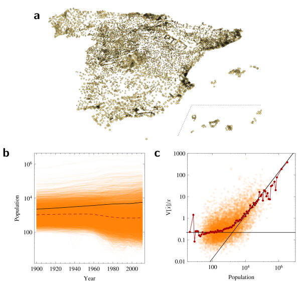
Figure 1: Characteristics of the dataset. a, Spatial distribution of Spanish Municipalities. Circle’s sizes are proportional to the population’s logarithm. b, Evolution of all municipalities. We give also the population per town (arithmetic mean in black and geometric mean in red). c, Variance of the population-change vs. population for each municipality (dots). The median value (red dot-line) clearly follows Eq. (4) (black line).

II.2 Empirical observation of inertial growth

To find whether there exists a systematic dependence between successive yearly growths (or inertia) we consider first the $n$-cities-average and variance such that

$$\langle\dot{x}(t)\rangle = \frac{1}{n}\sum_{i=1}^{n}\dot{x}_{i}(t),$$ (7)

$$V[\dot{x}(t)] = \frac{1}{n}\sum_{i=1}^{n}[\dot{x}_{i}(t)-\langle\dot{x}(t)\rangle]^{2},$$ (8)

where $x_{i}(t)=X_{i}(t)/N(t)$ with $N(t)$ the total population at time $t$, excluding in this fashion the effects of the total population growth. Time correlations have been obtained via the Pearson product-moment correlation coefficient (${\mathrm{Corr}}$) between data-sets pertaining to different years $t_{1}$ and $t_{2}$. The mean correlation as a function of the time interval $\Delta t=|t_{1}-t_{2}|$ is obtained as the average

$$c(\Delta t) = \frac{1}{T}\sum_{t=1}^{T}\mathrm{Corr}[\dot{x}(t),\dot{x}(t+\Delta t)]$$ (9)

$$= \frac{1}{T}\sum_{t=1}^{T}\frac{\mathrm{Cov}[\dot{x}(t),\dot{x}(t+\Delta t)]}{\sqrt{V[\dot{x}(t)]V[\dot{x}(t+\Delta t)]}},$$

where ${\mathrm{Cov}}(a,b)$ is the covariance between variables $a\,-\,b$ and $T$ is now the total number of available data-sets for each case. We study first such correlations as a function of the population window, where two different situations are encountered. Within a standard deviation, no correlations exist for low populations, but they are significative for large ones, as indicated by Fig. 2a. The transition between the two ensuing regimes takes place at populations of $\sim 1000$ inhabitants. Thus, for the finite size term in (4) no time correlations are detected. They do appear, though, in the proportional growth regime. Accordingly, we evaluate time-correlations for municipalities with populations of more that ten thousand inhabitants during a period of up to 50 years. We find that correlations decay as the time interval $\Delta t=|t_{1}-t_{2}|$ between observations increases (Fig. 2b). The resulting mean value can be nicely fitted by an exponential function

$$\langle{\mathrm{Corr}}(\Delta t)\rangle=c_{t}\exp(-\Delta t/\tau),$$ (10)

with $c_{t}=0.74\pm 0.02$ and $\tau=15\pm 1$ years. Accordingly, the correlation’s mean-time in the demographic flux is of around 15 years.

II.3 Empirical observation of spatial correlations.

We pass now to a study of the demographical entanglement between two given cities, as represented by spatial correlations. The correlation coefficient between the $i$-th and $j$-th city reads

$$c_{ij}=\mathrm{Corr}[\dot{x}_{i},\dot{x}_{j}]=\frac{\mathrm{Cov}[\dot{x}_{i},\dot{x}_{j}]}{\sqrt{V[\dot{x}_{i}]V[\dot{x}_{j}]}},$$ (11)

where the covariances, variances, and means are time-averages as in Eq. (5). Amongst a host of possible entanglement factors, we choose here to study the simplest one: distance between cities $\Delta r$. Accordingly, we evaluate correlations between cities versus their pertinent distance ${\mathrm{dist}}(i,j)$ via the histogram

$$\langle\mathrm{Corr}(\Delta r)\rangle=\frac{1}{n}\sum_{i=1}^{n}c_{ij}\delta(\Delta r-{\mathrm{dist}}(i,j)).$$ (12)

We find that for towns with more that 10000 inhabitants –within the proportional growth regime– the mean value of the spatial correlation does depend upon distance as a power law, but saturates for short distances. Things can be nicely fitted by the expression

$$\langle{\mathrm{Corr}}(\Delta r)\rangle=\frac{c_{r}}{1+|\Delta r/r_{0}|^{\alpha}},$$ (13)

obtaining $c_{r}=0.33\pm 0.02$, $r_{0}=76\pm 10$, and $\alpha=1.8\pm 0.3$, with a coefficient of determination $R^{2}$ equal to $0.9159$. Instead, fixing for future convenience $\alpha=2$, that yields a Lorentz function, we get $c_{r}=0.33\pm 0.01$ and $r_{0}=79\pm 8$, with $R^{2}=0.9156$. Since the concomitant two ways of fitting are indistinguishable, we adopt $\alpha=2$ for simplicity. As a consequence, the typical “demographic distance" turns out to be (in average) of $\sim 80$ km, decaying with $r^{-2}$ at large distances. Thus, we face long-range correlations (Fig. 2d). The influences of other factors, though, make these correlations to vanish at about 500 km. We use our data to compare i) the width of ${\mathrm{Corr}}(\Delta r)$ with ii) that expected for a bivariate normal distribution biv (see Appendix). The empiric width is larger than the bivariate one: $0.327$ vs. $0.204$ (Fig. 2c), indicative of the presence of additional, distance-independent, correlations. We deduce that the separation between towns, that is, their mutual distance, is the origin of about a 60% of the total correlation between them.

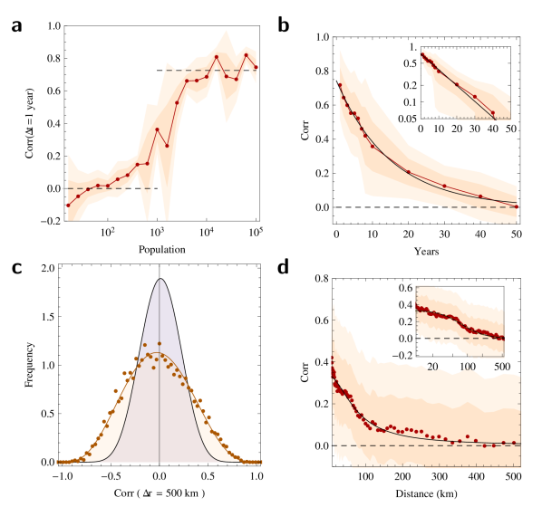
Figure 2: Empirical space-time correlations of population growth. a, Time-correlations versus town-sizes for yearly relative growths (red curve and red dots). The shaded area represents the width determined by one standard deviation (darker hue) and by two of them (lighter hue). Horizontal dark lines are just visual aids. b, Time correlation for the relative growth of towns populated by more that 10,000 inhabitants. Shaded areas represent widths determined by one (darker hue) and two (lighter hue) standard deviations, respectively. Inset: same representation, but in a log scale. The exponential fit of Eq. (10) acquires thus more visibility. c, Comparison of widths: bivariate-normal vs. empirical correlations-distribution. d, Spatial correlation of Spain’s municipalities’ relative growth for populations larger than 10,000 inhabitants. In black, the Lorentz shape of Eq. (13) (for $\alpha=2$) compared with the empirical mean (red dots). Inset: same representation, with a log scale for the distance.

II.4 Quantitative model for inertial and correlated urban growth

How to explain and reproduce these remarkable results? To such an end we advance here a model, compatible with previous descriptions and observations, inspired by the Langevin equation langevin . Accordingly, it includes inertia, ‘forces’ $F_{i}(t)$, and a friction-coefficient $\gamma$, whose values should fit empirical observation. Correlated forces imply a correlation matrix $Q_{ii^{\prime}}=\langle F_{i}(t)F_{i}^{\prime}(t)\rangle/V_{f}$, where $V_{f}$ is the variance of the forces, to be empirically adjusted. Disregarding finite-size noise one is led to

$$F_{i}(t) = \sum_{i^{\prime}=1}^{n}R_{ii^{\prime}}f_{i^{\prime}}(t),$$ (14)

$$\dot{v}_{i}(t) = F_{i}(t)-\gamma v_{i}(t),$$ (15)

$$\dot{u}_{i}(t) = v_{i}(t),$$ (16)

$$\dot{x}_{i}(t) = e^{u_{i}(t)},$$ (17)

where

• $f_{i}(t)$ are uncorrelated random forces such that ${\mathrm{Corr}}[f_{i}(t),f_{i^{\prime}}(t^{\prime})]=V_{f}\delta_{ii^{\prime}}\delta(t-t^{\prime})$ and

• $R_{ii^{\prime}}$ are the matrix elements of a correlation-generating matrix such that $\sum_{i^{\prime}j^{\prime}}R_{ii^{\prime}}R_{jj^{\prime}}=Q_{ij}$.

The form of $F_{i}(t)$ suggests that the force acting on a city is somewhat the average value of several independent ones. Now, an important personal decision is that of selecting to move to a certain location on the basis of available information. This information derives from human contacts of the concomitant individual, whose spatial distribution (SD) has been found to follow a $r^{-2}$ law at large distances, saturating for short ones gmodel . For simplicity, we assume a Lorentz shape for this SD

$$R_{ij}=\frac{R_{j}(0)}{1+|2\Delta r_{ij}/r_{0}|^{2}},$$ (18)

where $\Delta r_{ij}$ is the distance between the $i$ and $j$-th cities and the normalization constant is defined as

$$R_{j}(0)=\left[\sum_{k=1}^{n}(1+|2\Delta r_{kj}/r_{0}|^{2})^{-2}\right]^{-\frac{1}{2}}.$$ (19)

Thus, $F$ becomes a “coarse-grained" force. Let us consider for our derivation of $Q$ the continuous limit $x_{i}\rightarrow x(\mathbf{r})$, with $\mathbf{r}$ a planar spatial coordinate. $x(\mathbf{r})$ represents the relative population at $\mathbf{r}$, and the total normalized population becomes $1=\int_{S}d\mathbf{r}x(\mathbf{r}),$ where $S$ is the pertinent region’s area. Since we deal now with the coordinates $\mathbf{r}$ and $\mathbf{r}^{\prime}$ instead of the indexes $i,j$, the $R$ matrix-elements are a function $R(|\mathbf{r}-\mathbf{r}^{\prime}|)$. Sums become integrals obtaining $R(0)=2[2/\pi r_{0}^{2}]^{1/4}$ and the convolution ($\otimes$) for the coarse-grained force

$$F(\mathbf{r},t)=R(\mathbf{r})\otimes f(\mathbf{r},t)=\int_{S}d\mathbf{r}^{\prime}\frac{2[2/\pi r_{0}^{2}]^{1/4}f(\mathbf{r}^{\prime},t)}{1+4|(\mathbf{r}-\mathbf{r}^{\prime})/r_{0}|^{2}}.$$ (20)

Since the convolution of two Lorentzians of equal scale is also a Lorentzian with twice that scale-parameter, we find for the forces-correlation

$$\mathrm{Corr}[F(\mathbf{r}),F(\mathbf{r}^{\prime})] = Q(|\mathbf{r}-\mathbf{r}^{\prime}|)$$ (21)

$$= R(|\mathbf{r}-\mathbf{r}^{\prime}|)\otimes R(|\mathbf{r}-\mathbf{r}^{\prime}|)$$

$$= \frac{1}{1+|(\mathbf{r}-\mathbf{r}^{\prime})/r_{0}|^{2}}.$$

Thus we write for the general case

$$Q(\Delta r_{ij})=\frac{1}{1+|\Delta r_{ij}/r_{0}|^{2}}.$$ (22)

To obtain the correlation for the growth we solve Eqs. (14)-(17) for $v$ and $x$ writing

$$v_{i}(t) = e^{-\gamma t}v_{i}(0)+\int_{0}^{t}d\tau e^{-\gamma(t-\tau)}F_{i}(\tau).$$ (23)

$$x_{i}(t) = \exp\left[\frac{v_{i}(0)}{\gamma}(1-e^{-\gamma t})+\right.$$ (24)

$$\phantom{\exp\leavevmode\nobreak\ \leavevmode\nobreak\ }\left.\int_{0}^{t}d\tau\int_{0}^{\tau}d\tau^{\prime}e^{-\gamma(\tau-\tau^{\prime})}F_{i}(\tau^{\prime})\right].$$

We have then $C_{ij}(\Delta t)=\mathrm{Corr}[\dot{x}_{i}(t),\dot{x}_{j}(t+\Delta t)]=\mathrm{Corr}[v_{i}(t),v_{j}(t+\Delta t)]$. On the basis of that the initial time is arbitrary, we assume $t\rightarrow\infty$ so as to obtain the $v-$correlation

$$C_{ij}(\Delta t)=\mathrm{Corr}[v_{i}(t),v_{j}(t+\Delta t)]=\frac{e^{-\gamma\Delta t}}{1+|\Delta r_{ij}/r_{0}|^{2}}$$ (25)

which nicely reproduces empirical data with $\gamma=1/\tau$ (from the variance of $v_{i}(t)$ we also obtain $V_{f}/2\gamma=\sigma_{v}^{2}$).

Without trying to be exhaustive, we have tested our equations with a numerical experiment. One simulates a square (area) of 500$\times$500 km², and randomly place on it 1000 “virtual" cities (Fig. 3a). Using the empirical values for $r_{0}$, $\gamma$, and $V_{f}$, one makes the system to evolve during 100 years. All cities possess the same population at the beginning. The concomitant results are analyzed by recourse to the methods used above for dealing with empirical data. Comparisons are made with theoretical predictions and plotted in Fig. 3b and 3c for time and spatial correlations, respectively. Expectations are seen to be fulfilled. It is worth mentioning that we have followed a normal-modes description to solve the associated equations, working with collective, independent modes (see Appendix). Our virtual municipalities display the same behavior recorded for actual ones. The main difference ensues from the presence of (as yet) undefined correlations in the empirical data.

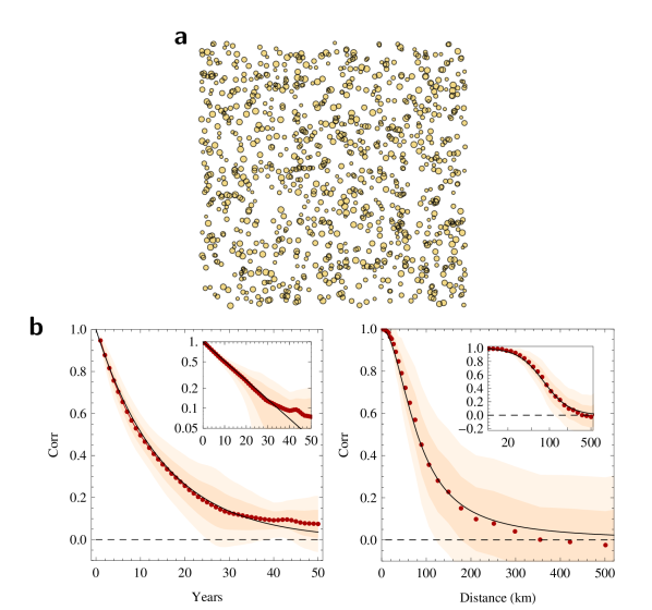
Figure 3: Numerical experiment solving Eqs.(14)-(17). a, Spatial distribution of “virtual" municipalities. Each side of the square represents 500 km. b, Time correlation for the relative growth of virtual towns. Shaded areas represent widths determined by one (darker hue) and two (lighter hue) standard deviations, respectively. Inset: same plot in a log scale. c, Spatial correlation of virtual municipalities’ relative growth. In black, the theoretical Lorentz shape of Eq. (22), compared with the empirical mean (red dots).

III Conclussion

Summing up, by recourse to the geometric walkers-model of Eqs. (14-17), we have empirically demonstrated that the relative growth of a city’s population exhibits both i) inertia and ii) correlation with the relative growth of neighboring cities, with distance as the main variable that underlies that town-town interaction. We also showed that a model inspired by the Langevin equation is able to reproduce these observations. Indeed, the model that we present here can be used to improve the predictive power of present techniques for demographic projection. However, further improvements are needed in order to identify the undefined correlations within the actual data whose existence we have discovered. We expect that these correlations will depend on local circumstances and also on the particular socio-economic status of each city.

Acknowledgments. This work was partially supported by Social Thermodynamics Applied Research (SThAR) (to AH and RH), and the project PIP1177 of CONICET (Argentina), and the projects FIS2008-00781/FIS (MICINN)-FEDER, EU, Spain (to AR).

Appendix A Distribution of correlation coefficients

For a bivariate normal distribution, the distribution of correlation coefficients is given by

$$P(c,C,T) = \frac{1}{\sqrt{2\pi}}(T-2)\frac{\Gamma(T-1)}{\Gamma(T-1/2)}(1-c^{2})^{T/2-2}\times$$ (26)

$$\left[1-C^{2}\right]^{(T-1)/2}\left[1-Cc\right]^{T-3/2}\times$$

$${}_{2}F_{1}\left[1/2,1/2,T-1/2,(Cc+1)/2\right],$$

where $c$ stands for the correlation-value that one might numerically obtain using Eq. (11), $C$ is the actual correlation value and $T$ the number of data-point used to evaluate $c$.

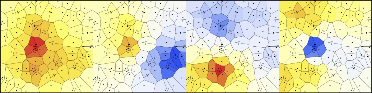
Figure 4: omponents of the first four eigenvectos of the simulated system (from white to red: positive values; from white to blue: negative values). The surface of each municipality is defined by its Voronoi area.

Appendix B The normal mode solution for the correlated Langevin equation

The computational cost of solving Eqs. (14)-(17) can be reduced via a normal-mode treatment. Indeed, we have defined a change-of-basis matrix $A$ such that $R$ (and $Q$) become diagonal. This generates new variables $u^{\prime}_{i}(t)=\sum_{i^{\prime}}A_{ii^{\prime}}\log[x_{i}(t)]$ whose motion-equations are

$$\dot{u}^{\prime}_{i}(t) = v^{\prime}_{i}(t),$$ (27)

$$\dot{v}^{\prime}_{i}(t) = \sqrt{\varepsilon_{i}}f^{\prime}_{i}(t)-\gamma v^{\prime}_{i}(t),$$ (28)

with $v^{\prime}_{i}(t)=\sum_{ii^{\prime}}A_{ii^{\prime}}v_{i}(t)$, $f^{\prime}_{i}(t)=\sum_{ii^{\prime}}A_{ii^{\prime}}f_{i}^{\prime}(t)$, and $\sqrt{\varepsilon_{i}}$ is the $i$-th eigenvalue of $R$ (with $\varepsilon_{i}$ that of $Q$). One easily checks that the forces $f^{\prime}$ are statistically equivalent to those indicated by $f$ (i.e., $\langle f^{\prime}_{i}(t)f^{\prime}_{j}(t+\Delta t)\rangle=V_{f}\delta_{ij}\delta(\Delta t)$ ), so that the simulation involves directly the random generation of $f^{\prime}$, without having to actually effect the basis-change. The variables $u^{\prime}_{i}(t)$ evolve in independent fashion, representing normal-mode evolution. The presence of $\sqrt{\varepsilon_{i}}$ accounts for different mode-equilibrations between $f^{\prime}$ and the dumping $\gamma$. This fact might be conceived as originating mass-factors. Figure 4 displays the first four modes for 100 cities distributed uniformly in a square of 100$\times$100 km using $r_{0}=30$ km, in such a way that the color at the Municipality $i$ represents the coefficient $A_{ii^{\prime}}$ for the eigenvector $i^{\prime}=$1, 2, 3 and 4 (the surface of each virtual municipality is in this example the Voronoi area).

References

- (1) Zipf GK (1949) Human Behavior and the Principle of Least Effort (Addison-Wesley, Cambridge, MA).
- (2) Kemeny J, Snell JL (1978) Mathematical Models in the Social Sciences (MIT Press, Cambridge, Mass.).
- (3) Marsil M, Yi-Cheng Zhang (1998) Interacting Individuals Leading to Zipf’s Law, Phys Rev Lett 80:2741.
- (4) Costa Filho RN, Almeida MP, Andrade JS, Moreira JE (1999) Scaling behavior in a proportional voting process, Phys Rev E 60:1067.
- (5) Axtell RL (2001) Zipf Distribution of U.S. Firm Sizes, Science 293:1818.
- (6) Blank A, Solomon S (2000) Power laws in cities population, financial markets and internet sites (scaling in systems with a variable number of components), Physica A 287:279.
- (7) Gabaix X, Ioannides YM (2004) Handbook of Regional and Urban Economics, Vol. 4 (North-Holland, Amsterdam).
- (8) Newman MEJ (2005) Power laws, Pareto distributions and Zipf’s law. Contemp Phys 46:323.
- (9) Newman MEJ, Barabasi AL, Watts DJ (2006) The Structure and Dynamics of Complex Networks (Princeton University Press, Princeton).
- (10) Bettencourt LMA, Lobo J, Helbing D, Kuehnert C, West GB (2007) Growth,. Innovation, Scaling, and the Pace of Life in Cities, Proc Natl Acad Sci USA 104 (17):7301-7306.
- (11) Batty M (2008) The Size, Scale, and Shape of Cities, Science 319:769.
- (12) González MC, Hidalgo CA, Barabási AL (2008) Understanding individual human mobility patterns. Nature 453:779-782.
- (13) Rozenfeld H, Rybski D, Andrade JS, Batty M, Stanley HE, Makse HA (2008) Laws of Population Growth, Proc Natl Acad Sci USA 105:18702.
- (14) Um J, Son SW, Lee SI, Jeong H, Kim JB (2009) Scaling laws between population and facility densities, Proc Natl Acad Sci USA 106 (34):14236-14240.
- (15) Castellano C,Fortunato S,Loreto V (2009) Statistical physics of social dynamics, Rev Mod Phys, 81:591.
- (16) Adamic L (2011) Unzipping Zipf’s law, Nature 474:165.
- (17) Simini F et al. (2012) A universal model for mobility and migration patterns, Nature, 484:96.
- (18) Hernando A et al. (2010) Unravelling the size distribution of social groups with information theory in complex networks, Eur Phys J B 76:87.
- (19) Hernando A, Plastino A (2013) Scale-invariance underlying the logistic equation and its social applications, Phys Lett A, 377:176.
- (20) Baek SK, Bernhardsson S, Minnhagen P (2011) Zipf’s law unzipped, New J Phys 13:043004.
- (21) Hernando A, Plastino A, Plastino AR (2012) MaxEnt and dynamical information, Eur Phys J B 85:147.
- (22) Hernando A, Plastino A (2012) Variational principle underlying scale invariant social systems, Eur Phys J B 85:293.
- (23) Hernando A, Plastino A (2012) The thermodynamics of urban population flows, Phys Rev E 86:066105.
- (24) Hernando A, Hernando R, Plastino A,Plastino AR (2013) The workings of the maximum entropy principle in collective human behaviour, J R Soc Interface 10:20120758.
- (25) Hernando A, Puigdomènech D, Villuendas D, Vesperinas C, Plastino A. (2009) Zipf’s law from a Fisher variational-principle, Phys Lett A 374:18.
- (26) Hernando A, Vesperinas C, Plastino A (2010) Fisher information and the thermodynamics of scale-invariant systems,Physica A, 389, 490.
- (27) Krings G, et al. (2009) Urban gravity: a model for inter-city telecommunication flows J Stat Mech L07003 doi:10.1088/1742-5468/2009/07/L07003
- (28) Plane DA, Henrie CJ, Perry MJ (2005) Migration up and down the urban hierarchy and across the life course,Proc Natl Acad Sci USA 102(43):15313-15318.
- (29) Willekens FJ, Drewe P (1984) A multiregional model for regional demographic projection, in Heide H, Willekens FJ, (ed) Demographic Research and Spatial Policy (Academic Press, London).
- (30) National Statistics Institute of Spain website, Government of Spain, www.ine.es.
- (31) Weisstein, Eric W. Bivariate Normal Distribution. From MathWorld-A Wolfram Web Resource. http://mathworld.wolfram.com/BivariateNormalDistribution.html
- (32) Coffey WT, Kalmylov YP (2004) The Langevin equation, with applications to stochastic problems in Physics, Chemistry and Electrical Engineering 3rd Edition, World Scientific Series in Contemporary Chemical Physics, Vol. 14.