Chemical Analysis of the Ninth Magnitude Carbon-Enhanced Metal-Poor Star BD+44^∘493 (catalog )

Abstract

We present detailed chemical abundances for the bright carbon-enhanced metal-poor (CEMP) star BD+44^∘493, previously reported on by Ito et al. Our measurements confirm that BD+44^∘493 is an extremely metal-poor ([Fe/H]$=-3.8$) subgiant star with excesses of carbon and oxygen. No significant excesses are found for nitrogen and neutron-capture elements (the latter of which place it in the CEMP-no class of stars). Other elements that we measure exhibit abundance patterns that are typical for non-CEMP extremely metal-poor stars. No evidence for variations of radial velocity have been found for this star. These results strongly suggest that the carbon enhancement in BD+44^∘493 is unlikely to have been produced by a companion asymptotic giant-branch star and transferred to the presently observed star, nor by pollution of its natal molecular cloud by rapidly-rotating, massive, mega metal-poor ([Fe/H] $<-6.0$) stars. A more likely possibility is that this star formed from gas polluted by the elements produced in a “faint” supernova, which underwent mixing and fallback, and only ejected small amounts of elements of metals beyond the lighter elements. The Li abundance of BD+44^∘493 ($A$(Li)=$\log$(Li/H)+12$=1.0$) is lower than the Spite plateau value, as found in other metal-poor subgiants. The upper limit on Be abundance ($A$(Be) =$\log$(Be/H)+12$<-1.8$) is as low as those found for stars with similarly extremely-low metallicity, indicating that the progenitors of carbon- (and oxygen-) enhanced stars are not significant sources of Be, or that Be is depleted in metal-poor subgiants with effective temperatures of $\sim$5400 K.

1 Introduction

The measured chemical abundances of extremely metal-poor (EMP; [FeH] $<-3.0$) stars are believed to reflect the early chemical enrichment of the Universe, in particular the yields of the first generations of massive stars. Stars at even lower metallicities (e.g., [Fe/H]$<-3.5$) exhibit other distinct characteristics. Among these: (1) The metallicity distribution function (MDF) shows evidence for a drop at [Fe/H]$\sim-3.5$ (e.g., Yong et al., 2012), though not as sharp a cutoff as that suggested by some previous studies (Schörck et al., 2009); (2) The fraction of carbon-enhanced metal-poor (CEMP) stars is quite high, on the order of 40% according to Beers & Christlieb 2005, and other recent determinations; and (3) there exist a number of “outliers” exhibiting chemical abundance ratios that are not often seen for relatively more metal-rich stars (excess of Mg, deficiency of Si, etc.; see Ryan et al., 1996; Norris et al., 2001; Johnson, 2002; Cayrel et al., 2004; Cohen et al., 2008; Lai et al., 2008; Yong et al., 2012).

Although great progress has been made over the past few decades by searches for very metal-poor stars in the halo (see Ivezić et al., 2012, for a recent review), the number of stars known to have metallicities below [Fe/H] = $-3.5$ is still rather small, probably reflecting the nature of the halo system’s MDF. For example, the most recent update of the SAGA database for chemical abundances of metal-poor stars (Suda et al. (2008) includes less than 30 objects with [Fe/H] $<-3.5$; a number of others have recently been added by Yong et al. (2012) and Aoki et al. (2012)). This makes the discovery of the nature of BD+44^∘493 rather remarkable (Ito et al., 2009), given that it is some three magnitudes brighter than the next example of such extreme stars. As shown by Ito et al. (2009), this star is a subgiant with [Fe/H]$=-3.8$, exhibits clear over-abundances of carbon and oxygen, and a lack of enrichment among the neutron-capture elements, placing it within the sub-class of CEMP-no stars (see Beers & Christlieb 2005). Thanks to its relative brightness, the abundances of other important elements that can constrain the possible progenitors of this star can be determined. For example, here we report a strong upper limit for Be, which is measurable only in the near-UV spectral region. The Be abundance for this star, as well as the abundance of Li, are useful for constraining mixing processes that might have occured in this star, and/or the formation process of these light elements in the early Universe. The rather low upper limit we obtain for lead ($\log\epsilon$(Pb)$<-0.10$) is of particular note, as previous predictions have suggested that, for stars as low in [Fe/H] as BD+44^∘493, one would have expected log$\epsilon$(Pb) $\sim+1.5$ (Cohen et al., 2006) from s-process.

This paper is outlined as follows. In § 2 we report details of the observations, reductions, and measurements of the spectral data, as well as related data used for our study, including derived kinematics. The determination of stellar parameters and chemical abundance analyses are reported in § 3 and § 4. In § 5, implications of the abundance results for BD+44^∘493 derived by our analyses are discussed, focusing on the origin of carbon and oxygen excess and the light elements Li and Be.

2 Observations and Measurements

2.1 High-Resolution Spectroscopy

BD+44^∘493 (catalog ) was observed with the HDS (High Dispersion Spectrograph; Noguchi et al. 2002) at the Subaru Telescope in 2008 August, October, and November, during an open-use intensive program (PI: W. Aoki) for high-resolution follow-up spectroscopy of very and extremely metal-poor stars discovered with the SDSS/SEGUE survey (Yanny et al., 2009). In addition to targets from SEGUE, some brighter very metal-poor candidates were also observed during twilight. The star BD+44^∘493 (catalog ) was first observed with a 10 minute exposure at dawn of 2008 August 22 (Hawaii Standard Time). The grating setting covered 4030-6730 Å, and the slit width was 0.6 arcsec (a $2\times 2$ on-chip binning was applied), yielding a resolving power of $R\sim 60,000$. Our initial abundance analysis of this spectrum surprisingly indicated that the metallicity of the star was $\mathrm{[Fe/H]}<-3.5$, which inspired a more detailed study of this object.

In 2008 October, we observed BD+44^∘493 (catalog ) again, using longer exposures, a wider wavelength coverage, and higher spectral resolution. Three different grating settings were used in order to cover 3080–9370  Å. We employed an 0.4 arcsec slit width (and no on-chip binning), achieving a resolving power of $R\sim 90,000$ . The total exposure time was 120 minutes for the near-UV setting, while 20 and 25 minute exposure times were used for the redder grating settings. We also observed a rapidly rotating B-type star (HD 12534 (catalog )) with the same settings as a reference for the elimination of telluric features. In order to obtain a spectrum over the wavelength range 3900–3960 Å, which fell in the CCD gap in the October run, an additional observation was carried out in 2008 November with a setting that covers 3540–5240  Å, using an exposure time of 5 minutes, an 0.6 arcsec slit (and $2\times 2$ on-chip binning), with a resulting resolving power of $R\sim 60,000$. Details of the observations are provided in Table 1.

Since the data from the October run are the highest quality, we mainly use them in this study. The November data are used for the analysis of some atomic lines at 3900–3960 Å, and for measurement of the radial velocity. A spectral atlas is provided as online material (see Appendix). The August data are used only for a radial-velocity measurement.

We carried out data reduction with the IRAF echelle package, performing overscan subtraction, CCD linearity correction (Tajitsu et al., 2010), cosmic-ray removal (see §2.2 in Aoki et al. 2005), division by the normalized flat-field exposures, extraction of the echelle orders, wavelength calibration, continuum normalization, and combining of all overlapping orders. The data in pixels affected by bad columns were removed.

The signal-to-noise ratio (S/N) per 0.9 km s^-1 pixel is estimated as the square root of the photon counts. For the October spectrum, a maximum S/N of 550/1 is achieved at 4700 Å, where the two grating settings overlap. The S/N decreases at shorter wavelengths to 300/1 at 3700 Å, and to 100/1 at 3100 Å. At 4800-7000 Å, a S/N of 200–300 is achieved. In the near-IR range ($>7000$ Å), the effective S/N declines to $\sim 100$, due to fringing on the CCD. Note that these S/N values should be multiplied by a factor of $\sim 1.9$ in order to obtain the S/N per resolution element, which is covered with $\sim 3.5$ pixels for a resolving power of $R\sim$90,000.

The August spectrum has a S/N per 1.8 km s^-1 pixel of 300/1 redder than $5500$ Å, decreasing to 200/1 at 4350 Å, and 150/1 at 4100 Å. For the November spectrum, the S/N is 200/1 redder than $4900$ Å, 130/1 at 3900 - 3960 Å, and 70/1 at 3570 Å. With a resolving power of $R\sim$ 60,000 (and $2\times 2$ on-chip binning), the S/N per resolution element is $\sim 1.6$ times larger than the S/N per pixel.

2.2 Line Measurements

We are in the process of compiling a large master line list of data from used by various studies (Aoki et al., in preparation); this line data is complemented in the near-UV region by the line lists employed in several other abundance studies of extremely metal-poor stars (Frebel et al., 2007b; Honda et al., 2006; Cohen et al., 2008; Lai et al., 2008). We make use of this list for our present analysis.

The equivalent widths of unblended lines, measured by a Gaussian fitting procedure, are employed to determine chemical abundances as described in §4. The atomic data and measured equivalent widths are listed in Table 2. The error of the equivalent width measurement is estimated as $\sigma_{\mathrm{EW}}=wn_{\mathrm{pix}}^{1/2}/(\mathrm{S/N})$, where $w$ is the pixel width (Å), $n_{\mathrm{pix}}$ is the number of pixels across the line, and S/N is the signal-to-noise ratio per pixel (Norris et al., 2001). Applying this formula, the errors of our measurements are estimated to be smaller than $0.1$ mÅ for most of the measured lines, and at most $0.4$ mÅ for some individual cases.

For several undetected lines, we list upper limits on the equivalent widths in Table 2, estimated with a spectrum synthesis approach. We also employ the spectrum synthesis technique for blended lines and molecular features. Details are described in §4.

2.3 Radial Velocity

Heliocentric radial velocities were measured for the high-resolution spectra obtained at four different epochs: 2008 August 22, 2008 October 4, 2008 October 5, and 2008 November 16. The spectrum obtained with the reddest setting in October 4 is not used, because the number of detected lines that can be employed for the measurement is too small in that wavelength range. We use 16 isolated Fe I lines in the wavelength regions 4030–4350 Å and 4420–4780 Å, which are covered by all of the spectra for the four epochs, in order to measure the radial velocities. The observed velocities are corrected for the motion of the Earth, then converted to heliocentric radial velocities. The resultant radial velocities and HJD (Heliocentric Julian Date) are listed in Table 3.

Random errors in the radial velocity measurements are estimated as $\sigma=sN^{-1/2}$, where $s$ is the sample standard deviation and $N$ is the number of lines used ($N=16$). The derived random error is typically $0.03\,\mathrm{km\,s^{-1}}$. Therefore, the total error is dominated by the systematic error due to the instability of the instrument, which is estimated to be about $0.5\,\mathrm{km\,s^{-1}}$.

We find no clear variation of the heliocentric radial velocity for BD+44^∘493 from 2008 August 22 to 2008 November 16. Furthermore, our measurements agree (within the reported errors) with the results of the extended radial velocity monitoring of BD+44^∘493 from 1984 to 1997 reported by Carney et al. (2003); the results of both Carney et al. (2003) and our measurements are shown in Figure 1. Carney et al. (2003) investigated the possibility of radial velocity variations for their sample, including BD+44^∘493. The ($E/I$) of BD+44^∘493 is close to unity, indicating that the scatter of the radial velocity (the “rms external error” $E$) is mostly explained by mean internal error of measurements ($I$). The $P(\chi^{2})$ value (0.23) for BD+44^∘493, which is significantly larger than the values of known binary stars, also indicates that the radial velocity scatter is explained by internal errors. Hence, though no useful data exist between their measurements and ours, no signature of radial velocity variation is found for BD+44^∘493 over 24 years (rms = 0.73 km s^-1), indicating that it is either not a binary star, or it is one with an extremely long period.

2.4 Interstellar Absorption

As shown in Figure 2, we detect a clear single component of interstellar absorption associated with both the individual Na I D1 and D2 lines. The observed wavelengths, heliocentric radial velocities, and equivalent widths, which were measured by fitting Gaussian profiles, are presented in Table 4. We confirm that the equivalent widths measured by direct integration differ by less than 5% from those obtained by Gaussian fitting.

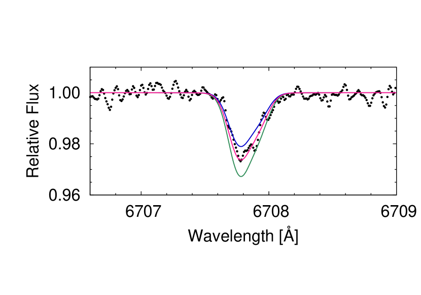
Figure 7: Observed spectrum (dots) and synthetic spectra (lines) for the Li I doublet at 6708 Å. Assumed abundances are $\log\epsilon(\mathrm{Li})=+0.95$, +1.00, and +1.05.

According to the relationship between the equivalent widths of the interstellar Na I D2 line and distance shown in Figure 7 of Hobbs (1974), a lower limit on the distance to BD+44^∘493 is estimated to be about 200 pc. This result is consistent with the distance derived from the stars geometric parallax (205 pc; see §2.5).

The color excess for BD+44^∘493 is estimated to be $E(B\!-\!V)=0.042$, based on empirical relations between the equivalent width of the interstellar Na I D2 line and $E(B\!-\!V)$ provided in Table 2 of Munari & Zwitter (1997).

2.5 Parallax, Proper Motion, and Kinematics

The parallax and proper motion of BD+44^∘493 were measured by the Hipparcos mission. We adopt the results of the new reduction (van Leeuwen, 2007), which are listed in Table 5. The parallax of $4.88\pm 1.06$ mas indicates the distance of $205\,^{+57}_{-37}$ pc.

The orbital parameters of this star (Table 6) are calculated for the above data and the radial velocity of BD+44^∘493, following the procedures of Carollo et al. (2010). The Galactocentic rotational velocity, $V_{\phi}$, of BD+44^∘493, its derived $Z_{\rm max}$ (the maximum distance from the Galactic plane reached during its orbit), and its orbital eccentricity, $e$, are typical for values associated with objects belonging to the inner-halo population, even though most stars with such extremely low metallicity are usually members of the outer-halo population (Carollo et al., 2010). The kinematic separation into these populations is, however, meaningful only in a statistical sense, and is not definitive for individual objects. Indeed, the outer-halo population has a large dispersion in its orbital parameters, and this star may just be in the tail of the distribution.

2.6 Photometry Data

We present available photometry for BD+44^∘493 in Table 7. Values for the $B_{T}$ and $V_{T}$ photometry are taken from the Tycho-2 Catalog (Hog et al., 2000). Empirical relations between the Johnson $BV$ magnitudes and Hipparcos-Tycho $B_{T}V_{T}$ magnitudes are presented in Bessell (2000). The near-IR $JHK_{s}$ magnitudes are from the 2MASS All-Sky Catalog of Point Sources (Cutri et al., 2003), while the value of the $b\!-\!y$ color and Balmer discontinuity index $c_{1}=(u\!-\!v)-(\!v-\!b)$ are from the uvby$\beta$ Catalog (Hauck & Mermilliod, 1998). Note that the errors on $b\!-\!y\,,\,c_{1}$ listed in Table 7 are random errors, and do not include systematic errors.

The reddening maps of Schlegel et al. (1998) and Burstein & Heiles (1982) yield $E(B\!-\!V)=0.092$ and $E(B\!-\!V)=0.115$, respectively, along the line of sight toward BD+44^∘493 (catalog ). However, taking the short distance to BD+44^∘493 into account, these estimates represent upper limits to the true reddening. Following Anthony-Twarog & Twarog (1994), we reduced these estimates by the fraction $f=1-\exp(-Hr\sin|b|)$, where $r$ is the star’s distance, $b$ is the Galactic latitude, and $H$ is a constant defined by Bond (1980) as 0.008 pc^-1. Assigning $r=205$ pc, as described in §2.5, we obtain $f=0.34$. The resultant reddening estimates are $E(B\!-\!V)=0.031$ from the Schlegel et al. (1998) maps and $E(B\!-\!V)=0.039$ from the Burstein & Heiles (1982) maps.

Together with the estimate from the interstellar absorption features in the high-resolution spectrum of BD+44^∘493 presented in §2.4 (0.042), we adopt a straight average of these three estimates: $E(B\!-\!V)=0.037$. Reddening corrections for the other passbands are derived from $E(B\!-\!V)$ based on the relative extinctions given in Table 6 of Schlegel et al. (1998).

3 Stellar Parameters

3.1 Effective Temperature

To estimate the effective temperatures for BD+44^∘493 from dereddened color indices, we employ the procedures and temperature scales of Alonso et al. (1996, 1999, 2001), González Hernández & Bonifacio (2009), and Casagrande et al. (2010) Alonso et al. (1996, 1999, 2001) and González Hernández & Bonifacio (2009) provide the relations between $T_{\mathrm{eff}}$ and colors for both dwarfs and giants. Since BD+44^∘493 is a subgiant, we calculate temperatures for both cases. The Casagrande et al. (2010) scale applies to both dwarfs and subgiants.

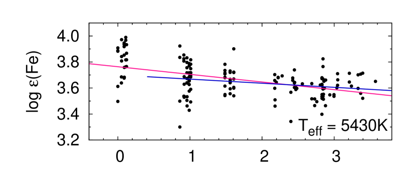
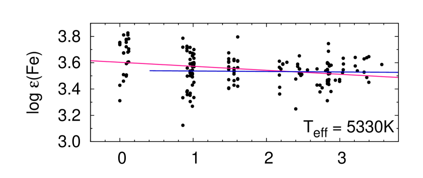
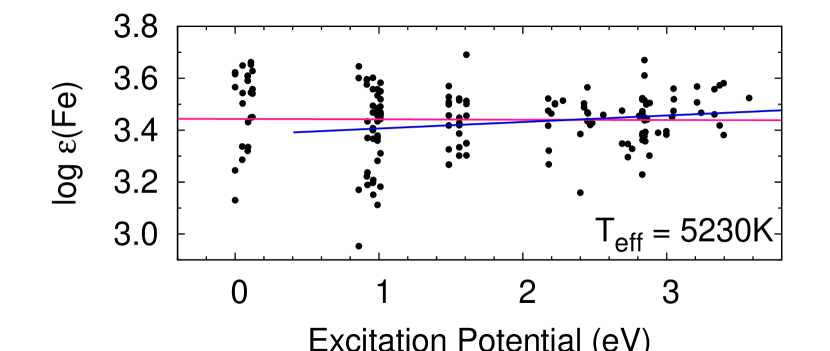
Figure 5: Fe abundances determined from individual Fe I lines, as a function of excitation potential. The upper panel is the case for our adopted temperature, $T_{\mathrm{eff}}=5430\,\mathrm{K}$, while the middle and lower panels apply for $T_{\mathrm{eff}}$ lower by $100\,\mathrm{K}$ and $200\,\mathrm{K}$, respectively. The longer lines indicate the fitted linear functions to all the points, while the shorter lines apply only to the points with $\chi>0.2\,\mathrm{eV}$.

Alonso et al. (1996) established the temperature scale for dwarfs, while Alonso et al. (1999, 2001) did so for giants. However, Ryan et al. (1999) pointed out that the temperature scales for dwarfs provided by Alonso et al. (1996) exhibit an unphysical metallicity dependence at low metallicity. Since the effect appears at $\mathrm{[Fe/H]}<-3.0$ (see Figure 5 in Ryan et al., 1999), we assume $\mathrm{[Fe/H]}=-3.0$ for BD+44^∘493 in the calculations both for the dwarf and the giant case; this assumption does not significantly affect the resultant temperatures.

The scales of González Hernández & Bonifacio (2009) are available over the metallicity range $-3.5\leq\mathrm{[Fe/H]}\leq+0.5$ for dwarfs, and over $-4.0\leq\mathrm{[Fe/H]}\leq+0.2$ for giants. We assume $\mathrm{[Fe/H]}=-3.5$ for the dwarf case, and $\mathrm{[Fe/H]}=-3.8$ for the giant case.

For the Casagrande et al. (2010) scales, we adopt $\mathrm{[Fe/H]}=-3.7$ for $b\!-\!y$, considering that the relation for the color is available in the range $-3.7\leq\mathrm{[Fe/H]}\leq+0.5$, and $\mathrm{[Fe/H]}=-3.8$ for the other colors.

Dereddened color indices are obtained from the photometry data and reddening estimates described in §2.6. The transformation of Hipparcos-Tycho $B_{T}V_{T}$ magnitudes into Johnson $BV$ is performed using the relations given in Table 2 from Bessell (2000). For the Alonso et al. (1996, 1999, 2001) calibrations, we transform the 2MASS $JHK_{s}$ magnitudes into the TCS (Telescopio Carlos Sanchez) system using Equation (1) in Ramírez & Meléndez (2004). Where possible, we dereddened the colors first and then transformed onto the required system.

All the dereddened and transformed colors are listed in Table 8, along with the derived temperatures. The uncertainties of the temperatures arising from the photometric errors are presented. Note that the small error on $T_{\mathrm{eff}}$ derived from $b\!-\!y$ is because the photometric error on $b\!-\!y$ does not consider systematic errors.

We rely primarily on the $V\!-\!K_{s}$ temperature estimated from Casagrande et al. (2010), and adopt an effective temperature of $5430\,\mathrm{K}$ for BD+44^∘493. The $V\!-\!K_{s}$ calibration is less sensitive to metallicity and photometric errors than is the case for other colors. Although the $(V\!-\!K_{s})_{0}$ color depends sensitively on the adopted reddening, we have obtained a very reliable reddening estimate for BD+44^∘493 (see §2.6) from multiple methods. The uncertainty due to the photometric errors are less than 50 K.

We note here that most of the other estimates listed in Table 8 are within $100\,\mathrm{K}$ of our adopted value. Exceptions are the values determined from $B-V$ and $J-H$. The $T_{\mathrm{eff}}$ scales from $B-V$ are not well-determined, partially because this color index is sensitive to metallicity. The $J-H$ color may not be a good indicator because the wavelength difference between the two bands is small, and the color index is less sensitive to $T_{\mathrm{eff}}$.

Effective temperature can also be determined by the constraint that the derived abundances of Fe from individual lines show no dependence on their excitation potentials. We investigate this in § 3.4.

Another constraint on $T_{\mathrm{eff}}$ is obtained from the profiles of Balmer lines, which are dependent on the temperature of the line-forming layers of stellar atmospheres, as well as on the surface gravity. The Balmer-line profiles calculated by Barklem et al. (2002) are compared with those of the observed spectrum. We give priority to the H$\beta$ line, because this line is not as sensitive to non-LTE effects as H$\alpha$ (Barklem, 2007), and the line is almost free from contamination from other spectral lines. Among the synthetic spectra calculated for $T_{\mathrm{eff}}$$=$5200–5600 K, $\log g$$=$3.5–3.8 and [Fe/H]$=-3.5$, the spectrum with $T_{\mathrm{eff}}$=5400 K shows the best agreement with the H_β profile of BD+44^∘493 in the wing regions (1–10 Å from the line center). The largest uncertainty is due to the continuum placement, which is accomplished in the manner described by Barklem et al. (2002), resulting in an uncertainty of $\pm 100$ K. Hence, we conclude $T_{\mathrm{eff}}$$=5400\pm 100$ K for this star. To be conservative, we use $\Delta T_{\mathrm{eff}}=150\,\mathrm{K}$ for obtaining estimates of the abundance uncertainties in §4.

3.2 Microturbulence

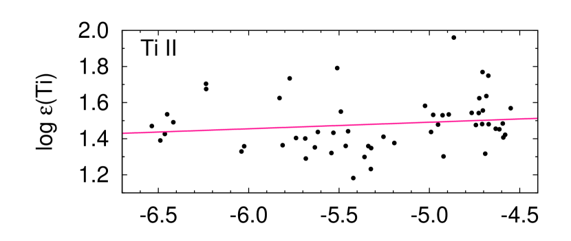
Figure 3: Derived Fe, Ti, and Ni abundances, as a function of the strength of each line. The solid lines indicate the fitted linear functions.

The microturbulent velocity, $v_{\mathrm{micro}}$, is derived from 158 Fe I lines by demanding that no trend is found for Fe abundances with line strengths, $\log(\mathrm{EW}/\lambda)$. In the upper panel of Figure 3, we illustrate the situation with the adopted value, $v_{\mathrm{micro}}=1.3\,\mathrm{km\,s^{-1}}$. The above effective temperature ($T_{\mathrm{eff}}$ = 5430 K) and $\log g$ = 3.4 (see below) are adopted in the calculations. No significant trend is found for 55 Ti II lines and 30 Ni I lines, as indicated in the middle and lower panels of Figure 3. The uncertainty of the microturbulence is estimated to be $0.3\,\mathrm{km\,s^{-1}}$.

3.3 Surface Gravity

Surface gravity is determined from the LTE ionization equilibrium of the Fe and Ti abundances, i.e., by requiring that the Fe and Ti abundances derived from neutral (Fe I, Ti I) and singly-ionized (Fe II, Ti II) lines be identical to within 0.02 dex, respectively. The ionization balance of both Fe I - Fe II and Ti I - Ti II is achieved simultaneously, when assuming $\log g=3.4$ in cgs units. We estimate an uncertainty of 0.3 dex in $\log g$, corresponding to uncertainties in the abundance determinations of $\sim 0.1$ dex.

Considering how non-LTE (NLTE) effects may change the result of Fe abundances, only Fe I lines are expected to suffer from significant NLTE corrections, while Fe II lines are almost immune to them (see Asplund et al. 2005 for a review). Although a consensus on the expected magnitude of the NLTE effects has not been reached, NLTE corrections for Fe I estimated by previous studies are about $+0.2$ dex at low metallicity. If we apply an NLTE correction for Fe I of $+0.2$ dex, the surface gravity needs to be increased by about $+0.4$ dex, resulting in $\log g=3.8$. Assuming this value, however, the Ti abundances from Ti I and Ti II lines result in a 0.1 dex disagreement.

We can also estimate the surface gravity from the parallax of BD+44^∘493 (see §2.5), employing the fundamental relation:

$$\log\frac{g}{g_{\odot}}=\log\frac{M}{M_{\odot}}+4\log\frac{T_{\mathrm{eff}}}{T_{\mathrm{eff}\odot}}+0.4(V_{0}+BC+5+5\log\pi\mathrm{[arcsec]}-M_{{\rm bol},\odot}),$$ (1)

where $M_{{\rm bol},\odot}$ is the absolute bolometric magnitude of the Sun (4.75). The stellar mass $M$ is assumed to be $0.8\,M_{\odot}$. The bolometric correction ($BC$) is derived using Equation (18) of Alonso et al. (1999), assuming $\mathrm{[Fe/H]}=-3.0$; the result is $-0.256$ mag. With our adopted temperature of $T_{\mathrm{eff}}=5430\,\mathrm{K}$, the measured parallax for BD+44^∘493 of $4.88\pm 1.06$ mas yields a $\log g=3.3\pm 0.2$, where the error of the parallax is the dominant error source. This agrees with our adopted value, $\log g=3.4\pm 0.3$, within the errors.

Figure 4 shows our adopted effective temperature and surface gravity, with error bars of $\Delta T_{\mathrm{eff}}=150\,\mathrm{K}$ and $\Delta\log g=0.3\,\mathrm{dex}$, compared with the Yonsei-Yale isochrone (Kim et al., 2002; Demarque et al., 2004), computed for an age of 12 Gyr, metallicity of $\mathrm{[Fe/H]}=-3.5$, and a 0.3 dex $\alpha$-element enhancement ($\mathrm{[\alpha/Fe]}=+0.3$). The isochrone indicates two possibilities for the derived effective temperature of BD+44^∘493 ($T_{\mathrm{eff}}=5430\,\mathrm{K}$): a subgiant case ($\log g\sim 3.1$) and a dwarf case ($\log g\sim 4.8$). Our LTE result is consistent with the subgiant case, while the dwarf case is clearly excluded. As described above, the NLTE correction for Fe I results in a higher surface gravity ($\log g\sim 3.8$), which corresponds to an unrealistic result, lying between the dwarf and subgiant cases, in the isochrone. This suggests that, in reality, the NLTE correction for Fe I is not as large as 0.2 dex.

3.4 Iron Abundance

We derived Fe abundances from 158 Fe I and 11 Fe II lines, following the descriptions in §4. Figure 6 shows Fe abundances determined from individual Fe I and Fe II lines, as a function of wavelength. The wide wavelength coverage and high quality of our spectrum allows us to investigate many lines, despite the low metallicity of this star. In particular, four Fe II lines at 3200 - 3300 Å with equivalent widths of more than 15 mÅ (see Table 2) are important for surface gravity determination from the Fe I / Fe II ionization equilibrium, since most optical Fe II lines are weak.

The upper panel of Figure 5 shows iron abundances determined from 158 measured Fe I lines, as a function of excitation potential. No trend is expected in such a plot, when the excitation equilibrium is satisfied. However, as indicated by the longer line in the upper panel of Figure 5, a slope of about $-0.06\;\mathrm{dex\;eV^{-1}}$ is found by fitting a linear function to all the points. This trend might imply that our photometric temperature is slightly too high.

Some previous studies of metal-poor stars, however, have also reported disagreement between photometrically-derived temperatures and spectroscopically-derived temperatures that are estimated so as to achieve excitation equilibrium (e.g., Cohen et al., 2008), and speculated that the problem arises from the use of lines with excitation potentials of $\chi\sim 0\,\mathrm{eV}$. If the fitting is performed using only the data points in $\chi>0.2\,\mathrm{eV}$, the slope becomes much shallower, although a weak trend remains (lines in the top panel of Figure 5), as also found by Lai et al. (2008) for their very metal-poor stars.

The slope found by fitting a linear function to the 133 points with $\chi>0.2\,\mathrm{eV}$ is $-0.033\pm 0.010\;\mathrm{dex\;eV^{-1}}$ when $T_{\mathrm{eff}}$$=5430$ K is adopted (the top panel of Figure 5). The null hypothesis that there is no correlation between the two values is rejected by the regression analysis at the 99.5% confidence level. If the abundance analysis is made assuming $T_{\mathrm{eff}}$$=5330\,\mathrm{K}$, no trend for the lines with $\chi>0.2\,\mathrm{eV}$ appears (the short line in the middle panel of Figure 5). The random error is estimated to be 50 K, adopting the 95% confidence level in the regression analysis.

We note for completeness that, in order to achieve the excitation equilibrium for all the lines, the temperature needs to be decreased by $200\,\mathrm{K}$ from the adopted value (see the bottom of Figure 5).

The $T_{\mathrm{eff}}$ estimated from the analysis of the Fe lines, assuming no dependence of Fe abundances on the excitation potential of individual lines, is $5330\pm 50$ K if the lines with $\chi\sim 0\,\mathrm{eV}$ are excluded. Although this is 100 K lower than the value estimated from the color index in § 3, as found for metal-poor stars by previous studies, the difference is still smaller than the error adopted in our analysis.

The derived abundances are $\mathrm{[Fe/H]}=-3.83$ from Fe I and $\mathrm{[Fe/H]}=-3.82$ from Fe II. In the following discussion, we adopt the result for Fe I, $\mathrm{[Fe/H]}=-3.83$, as our final iron abundance estimate for BD+44^∘493. Abundance errors for iron are described below in §4.

3.5 Adopted Stellar Parameters

We list our adopted stellar parameters and their uncertainties for BD+44^∘493, which are used for the abundance analysis, in Table 9. The adopted $T_{\mathrm{eff}}$ is 80 K lower than that adopted by Ito et al. (2009), who simply adopted the value of Carney et al. (2003). The surface gravity is lower by 0.3 dex than that of Ito et al. (2009), partially due to the lower $T_{\mathrm{eff}}$ adopted by the present work. The metallicity is also slightly lower than that of Ito et al. (2009), also due to the lower $T_{\mathrm{eff}}$ used in this work.

If the lower effective temperature suggested from the analysis of Fe I lines ($T_{\mathrm{eff}}$ = 5330 K, § 3.4) is adopted, $\log g$ = 3.2 and [Fe/H] $=-3.9$ are derived. The change of micro-turbulent velocity is smaller than 0.1 km s^-1. The $T_{\mathrm{eff}}$ and $\log g$ also agree within the errors with the subgiant branch of the isochrones shown in Fig. 4, although the data point lies slightly below the isochrones.

4 Abundance Analysis and Results

4.1 Abundance Determinations

We adopt one-dimensional LTE model atmospheres for the stellar parameters of BD+44^∘493, interpolating within the grid of ATLAS9 ODFNEW model atmospheres (Kurucz, 1993a; Castelli & Kurucz, 2003). The computed equivalent widths of spectral lines are compared with the observed ones listed in Table 2, in order to derive elemental abundances. The microturbulence velocity determined for BD+44^∘493 in §3 is adopted in the spectral line-formation calculations.

For molecular features and blended lines, we calculate synthetic spectra to compare with the observed spectrum directly, changing the abundance by 0.05 dex until the computed and observed spectra are well-matched. The spectrum synthesis code that we use is based on the same assumptions as the model atmosphere program of Tsuji (1978). We have assumed a Gaussian profile to account for the broadening by macroturbulence and the instrument, assuming that rotation is not a dominant source of the broadening. A broadening of $6.0\,\mathrm{km\,s^{-1}}$ is adopted for the profiles of single lines.

We also employ the spectrum synthesis approach to estimate upper limits on elemental abundances for several undetected lines. The upper limits are computed by comparing synthetic and observed spectra, and adjusting the abundance by 0.05 dex until the computed strength of the line is of the same order as the noise in the observed spectrum.

The derived abundances and upper limits are listed in Table 10. The number of lines used in the analysis is given in the third column. When only a single line or feature is available, the line or feature is given in the last column . Solar abundances are taken from Asplund et al. (2009) to obtain the abundance ratios ([X/Fe]). Details of the analyses for individual species are described below.

4.2 Abundance Errors

We estimate abundance errors, within the 1D LTE formalism, and list the results in Table 11.

Random errors arising from the measurements of atomic lines are estimated as $\sigma=s{N}^{-1/2}$, where $s$ is the sample standard deviation and $N$ is the number of lines used in the analysis. When the number of lines is too small to estimate a valid sample standard deviation (in the case of $N<10$), the $s$ derived from Fe I lines is used instead. For Li and the CNO elements, for which the spectrum synthesis approach is applied, random errors are estimated by taking into account continuum placement uncertainties, abundance variations from different features, and how well the synthetic spectrum fits the observed spectrum.

Abundance errors also come from the uncertainties in the stellar parameters. We examine them by performing abundance analyses after changing each stellar parameter (effective temperature, surface gravity, and microturblent velocity) by its uncertainty, as estimated in §3 (Table 11). The effect of the uncertainty in metallicity is negligible compared with those in the other parameters.

These errors are combined following the equation (2) of Johnson (2002) where the effects of correlations between parameters are included (Table 11). The covariances are calculated assuming Gaussian distribution with standard deviations of 150 K and 0.3 dex for $T_{\mathrm{eff}}$ and $\log g$, respectively. We found that the correlation between $T_{\mathrm{eff}}$ and $\log g$ have small impact on the total error, while effects of others are negligible. To estimate the $\sigma_{\rm total}$ of [X/Fe], changes of the abundance ratio ([X/Fe]) corresponding to the changes of individual parameters are adopted in the above calculation.

Possible NLTE and 3D effects are discussed for individual species in §4.3 - 4.7.

4.3 Light Elements: Li and Be

4.3.1 Lithium

We have employed spectrum synthesis to measure the lithium abundance for BD+44^∘493 from the Li I doublet at 6708 Å. Atomic data for these lines are taken from Smith et al. (1998); we assume no contribution from ⁶Li. Figure 7 shows the observed spectrum compared with synthetic spectra of different Li abundances. The derived result is $\log\epsilon(\mathrm{Li})=1.0$.

There are several studies on the effects of NLTE on Li abundances derived from the Li I doublet at 6708 Å. The most recent and sophisticated is by Lind et al. (2009), who performed NLTE calculations for a wide range of stellar parameters. For parameter sets similar to that of BD+44^∘493 ($T_{\mathrm{eff}}=5500\,\mathrm{K},\>\log g=[3.0,4.0],\>\mathrm{[Fe/H]}=-3.0,\>v_{\mathrm{micro}}=[1.0,2.0],\>\log\epsilon(\mathrm{Li})=[0.9,1.2]$), only very small NLTE corrections are suggested: $\log\epsilon(\mathrm{Li})_{\mathrm{NLTE}}-\log\epsilon(\mathrm{Li})_{\mathrm{LTE}}=[-0.02,0.00]$. This indicates that NLTE effects on the Li abundance of BD+44^∘493 have no significant impact.

Asplund et al. (2003) presented 3D NLTE calculations for Li abundances of two stars, and found that the 3D NLTE abundances were similar to the 1D NLTE results. Since the metallicity assumed in their calculation for the subgiant case in Asplund et al. (2003) is one order of magnitude higher than that of BD+44^∘493, further investigation of 3D NLTE corrections for the Li abundance is required to derive the final conclusion for BD+44^∘493. However, the Li in BD+44^∘493 is clearly lower than the value of the Spite plateau (A(Li) $\sim 2.2$; e.g., Meléndez et al. 2010).

4.3.2 Beryllium

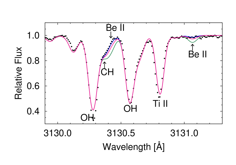
Figure 8: Same as Figure 7, but for Be II lines. Assumed abundances are $\log\epsilon(\mathrm{Be})=-2.1$, $-1.8$, and $-1.5$.

Our high-quality near-UV spectrum of BD+44^∘493 enables inspection of the Be II lines at 3130 Å. Although the lines are not detected in the spectrum, we set an upper limit on the Be abundance by spectrum synthesis. The line data used is based on Boesgaard et al. (1999) and the Kurucz line list. We do not include the two CH lines at 3131 Å given in Table 4 of Boesgaard et al. (1999), because no signature of these lines are found in our spectrum. Even if the Be II line at 3131 Å is removed in the calculations, the computed absorption strength at this wavelength exceeds the noise level of the observed spectrum due to these two CH lines. We note that this treatment results in a conservative upper limit for the Be abundance. Figure 8 compares the observed spectrum with synthetic spectra for different Be abundances. We estimate that the upper limit for the Be abundance is $\log\epsilon(\mathrm{Be})<-1.8$, and note that 3D and NLTE effects on the Beryllium abundance are expected to be small (Asplund, 2005).

4.4 C, N, and O abundances

The abundances of the elements C, N, and O are determined from molecular features (CH, NH, and OH) by comparison of the observed spectrum with synthetic spectra. The abundance measurements for nitrogen and oxygen are made by analyses of NH and OH lines in the wavelength range $<3400$ Å.

4.4.1 Carbon

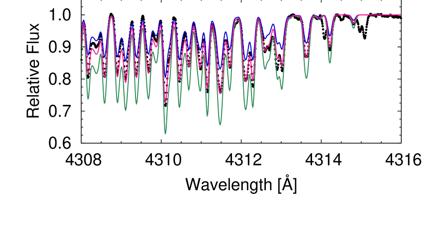
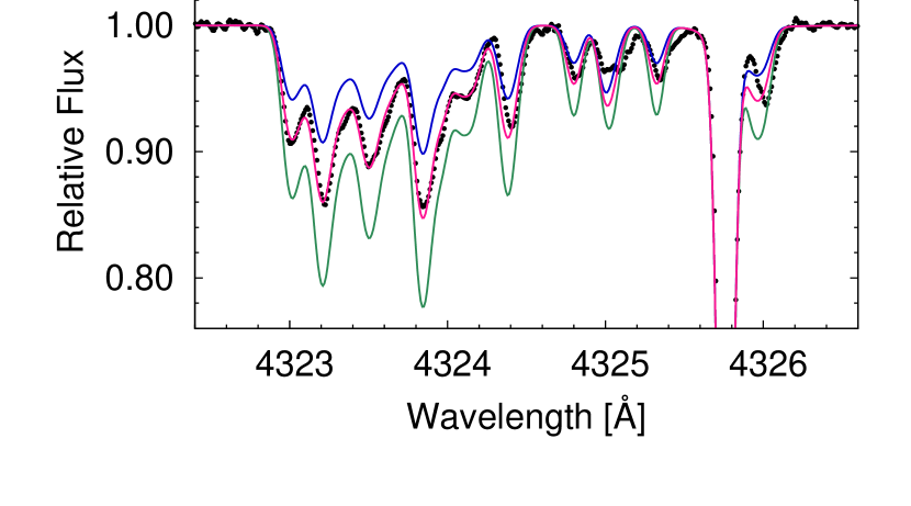
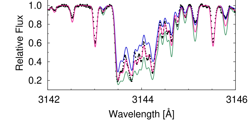
Figure 9: Same as Figure 7, but for the CH features at 4312 Å (top panel), 4324 Å (middle panel) and 3144 Å (bottom panel). Assumed abundances are $\mathrm{[C/Fe]}=+1.20$, +1.40, and +1.60 for the 4312 Å feature, $\mathrm{[C/Fe]}=+1.10$, +1.30, and +1.50 for that at 4324 Å, and $\mathrm{[C/Fe]}=+1.05$, +1.25, and +1.45.

We measure C abundances from the CH A-X features at 4312 Å and 4324 Å (Figure 9). Details of the line list used can be found in Aoki et al. (2006). The two C abundances differ by only about 0.1 dex. We take the straight average of them to obtain our final C abundance, $\mathrm{[C/Fe]}=+1.35$, indicating that BD+44^∘493 has a large excess of carbon.

We also synthesized spectra for a strong CH feature at 3144 Å, using the CH C-X line list based on Kurucz (1993b) (Figure 9, bottom panel). Since many OH lines exist at this wavelength region, and the accuracy of the line data is not well known, the C abundance from this feature is not as certain as those from the optical features. Hence, we do not include it in the final abundance result. However, the best fit is achieved for $\mathrm{[C/Fe]}=+1.25$, which is only 0.1 dex below the value estimated from the optical features. This supports the robustness of the C/O ratios derived by our analyses, in which the oxygen abundance is also derived from the OH lines in the near-UV range.

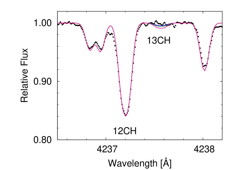
Figure 10: Same as Figure 7, but for ¹²CH and ¹³CH features at 4237 Å. Assumed ¹²C/¹³C ratios are 20, 30, and 40.

No feature of ¹³CH is detected in our spectrum of BD+44^∘493. A lower limit on the carbon isotope ratio (¹²C/¹³C) is estimated from the CH lines in 4215-4240 Å, as also done by Honda et al. (2004). An example is shown in Figure 10. The lower limit estimated from five features in this wavelength region is ¹²C/¹³C$>30$. Although the constraint is not strong, the result suggests that ¹²C production by the triple-$\alpha$ reaction dominates the contribution from the CNO cycle.

4.4.2 Nitrogen

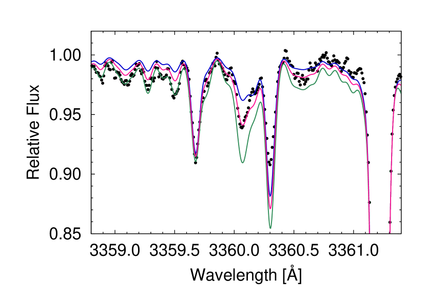
Figure 11: Same as Figure 7, but for NH features at 3360 Å. Assumed abundances are $\mathrm{[N/Fe]}=+0.25$, +0.45, and +0.65.

The N abundance is determined from the NH band feature at 3360 Å, using the NH line list based on Kurucz (1993b) (Figure 11). Aoki et al. (2006) modified the $gf$-values of the Kurucz (1993b) NH line list to reproduce the solar spectrum with the solar N abundance of Asplund et al. (2005). This modification produces a nitrogen abundance higher by +0.4 dex. Since our adopted solar N abundance (Asplund et al., 2009) is 0.05 dex lower than given in Asplund et al. (2005), we apply a correction of +0.35 dex. The final result is $\mathrm{[N/Fe]}=+0.40$, indicating that N is not significantly over-abundant in BD+44^∘493.

4.4.3 Oxygen

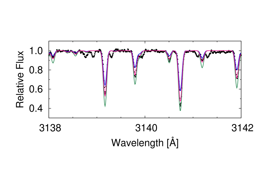
Figure 12: Same as Figure 7, but for OH features at 3140 Å. Assumed abundances are $\mathrm{[O/Fe]}=+1.44$, +1.64, and +1.84.

We measure 11 OH lines in the wavelength range 3120 - 3180 Å (3123.95, 3127.69, 3128.29, 3139.17, 3140.73, 3145.52, 3151.00, 3166.34, 3167.17, 3172.99, 3173.20 Å) to determine the O abundance, using the line list of Kurucz (1993b). An example of spectra including OH lines is shown in Figure 12. All the abundances determined from the individual lines agree with each other to within $\pm 0.2$ dex. A simple average is adopted as our final result: $\mathrm{[O/Fe]}=+1.64$. Thus, BD+44^∘493 is remarkably enhanced in oxygen.

Neither the forbidden [O I] line at 6300 Å, nor the O I triplet at 7772 Å, are detected in the observed spectrum of BD+44^∘493. We estimate upper limits on the O abundance from these lines, and obtain $\mathrm{[O/Fe]}<+2.34$ for the [O I] 6300 Å line, and $\mathrm{[O/Fe]}<+2.14$ for the O I 7772 Å line. These upper limits are not inconsistent with the O abundance determined from the OH lines in the UV regions.

Some previous studies discuss the discrepancies between the O abundances determined from the three different indicators: the OH band, the forbidden [O I] line, and O I lines (e.g., Israelian et al., 2001; García Pérez et al., 2006). No constraint on this issue is obtained for BD+44^∘493, as only weak upper limits are obtained from the [O I] and O I lines.

4.4.4 Possible 3D and NLTE effects

Recent calculations based on 3D hydrodynamical model atmospheres suggest that the CH, NH, and OH bands can be severely affected by 3D effects at low metallicity (see Asplund 2005 for a review). The 3D models yield much lower abundances than 1D models, and the magnitude can amount to as much as $-0.9$ dex at $\mathrm{[Fe/H]}=-3$ (e.g., Asplund & García Pérez 2001). This is because molecule formation in the cool regions occurs in the upper layers of the atmospheres in the 3D case. Although NLTE calculations result in higher abundances, they do not appear to fully compensate for the 3D effects. Thus, we might overestimate the CNO abundances in our 1D LTE analysis. However, it should be noted that the 3D and NLTE effects are expected to be more or less similar for the CH, NH, and OH bands, and abundance ratios among the three elements (e.g., C/O) are comparatively robust. We also note that carbon and oxygen abundances in EMP stars have been determined from CH and OH molecular features, as done for BD+44^∘493 in the present work. Hence, the excesses of these elements for this star are clearly evident.

4.5 Even-Z Elements: Mg, Si, S, Ca, and Ti

The Mg abundance is determined from eight Mg I lines in the wavelenth range 3800 - 5600 Å ($\mathrm{[Mg/Fe]}=+0.46$). Agreement of the results from the eight lines is fairly good. Recently, Andrievsky et al. (2010) performed NLTE calculations for Mg I lines for a large sample of metal-poor stars, and derived 0.3 dex higher Mg abundances for both giants and dwarfs at $\mathrm{[Fe/H]}\sim-3$. Our Mg abundance will also be increased if NLTE effects are taken into account.

Since the Si I line at 3906 Å falls in the CCD gap in the October spectrum, we use the November spectrum for the Si abundance measurement. Although the quality of that spectrum is not as high as that of the October spectrum (as stated in §2), it is sufficient for a clear detection of this line. We derive a Si abundance ratio $\mathrm{[Si/Fe]}=+0.49$. The blend with the CH lines is not severe at this wavelength, and Gaussian fitting to the Si I line works well. The NLTE effect on the line is expected to be small ($<0.1$ dex) for the effective temperature of BD+44^∘493 (Shi et al., 2009).

We have searched for the strongest S I lines at 9213 Å and 9237 Å in the wavelength range of our spectrum (3080 - 9370 Å), but find no feature at 9213 Å, and unfortunately, the 9237 Å line falls in the echelle order gap. The estimated upper limit on the S abundance from the 9213 Å line is $\mathrm{[S/Fe]}<+1.06$. According to Takeda et al. (2005), the NLTE correction for the line varies greatly with stellar parameters. For BD+44^∘493 it may reach about $-0.3$ dex.

In addition to the Ca I lines in the wavelength range 4220 -  6440 Å, we employed the Ca II line at 3181 Å and the strong Ca II triplet at 8490 - 8670 Å to derive the Ca abundance. These three indicators yield different results, $\mathrm{[Ca/Fe]}=+0.31$, +0.47, and +0.91, respectively. In particular, the large discrepancy between the Ca abundance obtained from the Ca I lines and the Ca II triplet cannot be explained by random errors (see Table 11). The NLTE calculations conducted by Mashonkina et al. (2007) result in increases of the abundance from Ca I lines by more than 0.2 dex, while the abundances estimated from the Ca II triplet decrease by about 0.3 dex, for similar parameter sets as BD+44^∘493. We adopt the Ca I lines as the abundance indicator in this paper in order to compare it with previous studies, most of which have adopted Ca I lines for their analyses.

We detect a number of Ti II lines, and several weak Ti I lines, in the observed spectrum. The ionization equilibrium is for this element is satisfied by our $\log g$ (see §3.3). The derived Ti abundance ratio is $\mathrm{[Ti/Fe]}=+0.36$. Unfortunately, we could find no NLTE study on Ti for extremely metal-poor stars discussed in the literature.

The abundances of the $\alpha$-elements Mg, Si, Ca, and Ti are enhanced by $\sim$ 0.3 - 0.5 dex with respect to Fe, as found for most of very and extremely metal-poor stars of the Milky Way halo.

4.6 Odd-Z Elements: Na, Al, K, and Sc

We determine the Na abundance ratio from the Na I D resonance lines at 5890 Å, and obtain $\mathrm{[Na/Fe]}=+0.30$. Andrievsky et al. (2007) suggested an NLTE correction of about $-0.1$ dex on the D lines for similar stellar parameters as BD+44^∘493.

The only available line that could be used for an Al abundance determination is the Al I resonance line at 3961 Å, yielding $\mathrm{[Al/Fe]}=-0.56$. We do not use the Al I line at 3944  Å, due to blending by CH lines. The Al abundance is quite sensitive to NLTE effects. From inspection of Figure 2 in Andrievsky et al. (2008), the NLTE correction for BD+44^∘493 probably exceeds $+0.5$ dex, and may amount to as much as $+0.7$ dex. Hence, Al is not as under-abundant as found by the LTE analysis.

The K abundance can be estimated from the K I doublet at 7665 Å and 7699 Å. However, in the observed spectrum of BD+44^∘493, the stronger feature at 7665 Å is unfortunately superimposed on large telluric lines. Although we attempted to remove the telluric features, we were not successful for these strong lines. We inspect the spectrum at 7699 Å, and set an upper limit on the K abundance of $\mathrm{[K/Fe]}<+0.75$. According to recent NLTE calculations, K abundances are overestimated in LTE computations. Takeda et al. (2009) and Andrievsky et al. (2010) derived NLTE K abundances for the same sample of metal-poor giants, which was originally studied under LTE by Cayrel et al. (2004), and reached similar conclusions. According to their estimates, the NLTE effect in EMP stars is not as large as in less metal-poor stars.

We used 12 Sc II lines in the wavelength range 3350 - 4420  Å to determine the Sc abundance, finding $\mathrm{[Sc/Fe]}=+0.29$. We do not take into account the effects of hyperfine splitting, which are expected to be negligible in an analysis of weak lines. No NLTE calculations for Sc for EMP stars are available in literature.

4.7 Iron-Peak Elements: V, Cr, Mn, Co, Ni, Cu, and Zn

Vanadium abundances have not been reported for many metal-poor stars, because even the strongest V I line in the optical at 4379 Å is difficult to detect. The line is also not detected in our spectrum of BD+44^∘493, and we estimate the upper limit on the V abundance ratio to be $\mathrm{[V/Fe]}<+0.20$. On the other hand, our near-UV spectrum permits measurements from two detectable V II lines at 3545 Å and 3592 Å. The derived V abundance ratio is $\mathrm{[V/Fe]}=-0.02$, which is consistent with the result from the V I line. We may need to exercise caution when comparing our V abundance determined from the V II with those determined from V I for other stars, given the result of Johnson (2002) that V II lines yielded about 0.2 dex higher V abundances than that from V I lines, although Lai et al. (2008) did not report such an offset.

The Cr abundance is measured from six Cr I lines and two Cr II lines. The resultant abundance from Cr II is 0.15 dex higher than that obtained from Cr I. Although measurements of Cr II lines are limited in previous studies of metal-poor stars, as the detectable lines are located at the near-UV region ($<3500$ Å), several studies found similar discrepancies (Frebel et al., 2007b; Lai et al., 2008; Bonifacio et al., 2009). Johnson (2002) reported a similar offset associated with optical Cr II lines for mildly metal-poor stars. We refer to the Cr I result as our final Cr abundance ratio, $\mathrm{[Cr/Fe]}=-0.37$.

We measure the Mn abundances from two Mn I lines at 4030 Å and three Mn II lines in the wavelength range 3440 - 3490  Å. The effects of hyperfine splitting are neglected because these lines are quite weak. The Mn II results are 0.3 dex higher than the Mn I results (Table 10). Cayrel et al. (2004) found that Mn abundances derived from the Mn I resonance triplet at 4033 Å are systematically lower than those from other lines, and corrected their Mn abundances from the triplet by +0.4 dex. Frebel et al. (2007b) and Bonifacio et al. (2009) also followed this procedure. Bergemann & Gehren (2008) suggested that the discrepancy is due to NLTE effects. Their NLTE calculations indicate that the abundance corrections for the Mn I triplet are 0.2 dex higher than those for other Mn I lines, although the difference does not reach 0.4 dex. Thus, NLTE effects might resolve the 0.3 dex disagreement between the Mn abundance ratios determined for BD+44^∘493 from the Mn I and Mn II lines. We here adopt the result from the Mn II lines, $\mathrm{[Mn/Fe]}=-0.79$.

A number of Co I and Ni I lines are used to obtain the Co and Ni abundance ratios, respectively ($\mathrm{[Co/Fe]}=+0.54$, $\mathrm{[Ni/Fe]}=+0.08$). The Co I lines could be severely affected by NLTE. According to Bergemann et al. (2010), the NLTE analysis increases Co abundances by as much as 0.7 dex at $\mathrm{[Fe/H]}=-3$ compared to the LTE analysis.

Thanks to our high-quality near-UV spectrum, we are able to measure two Cu I lines at 3248 Å and 3274 Å, resulting in an abundance ratio of $\mathrm{[Cu/Fe]}=-0.91$.

Zn is not detected in the observed spectrum. From inspection of the strongest Zn I line at 3345 Å, we set an upper limit on its abundance ratio of $\mathrm{[Zn/Fe]}<+0.17$.

4.8 Neutron-Capture Elements: Sr, Y, Zr, Ba, Eu, and Pb

The Sr abundance ratio is derived from the Sr II resonance lines at 4077 Å and 4215 Å, $\mathrm{[Sr/Fe]}=-0.23$. NLTE corrections for the Sr II lines depend on the adopted stellar parameters, and are positive for some stars, ane negative for others (Mashonkina & Gehren, 2001; Mashonkina et al., 2008; Andrievsky et al., 2011). In any case, it appears that these corrections would not be large ($<0.1$ dex).

We determine the Y abundance ratio from the Y II line at 3601 Å, and the Zr abundance ratio from the Zr II lines at 3438 Å and 3552 Å. The results are $\mathrm{[Y/Fe]}=-0.24$, and $\mathrm{[Zr/Fe]}=+0.04$. We clearly detect the Y II line at 3774 Å but do not use it, because it overlaps with a nearby Balmer line.

The Ba abundance ratio, $\mathrm{[Ba/Fe]}=-0.60$, is derived from the Ba II lines at 4554 Å and 4934 Å. We take hyperfine splitting into account, using the line list of McWilliam (1998), and assuming the isotope ratios of the $r$-process component of Solar System material. Andrievsky et al. (2009) performed NLTE calculations for Ba II, and obtained about 0.1 dex higher Ba abundances than LTE analyses for EMP dwarfs with $T_{\mathrm{eff}}=5500\,\mathrm{K}$. For giants with the same metallicity and temperature, the NLTE correction amounts to 0.2 dex or more. However, even if the NLTE effect is considered, Ba remains under-abundant in BD+44^∘493.

No Eu line is detected in the observed spectrum. From inspection of the Eu II line at 3820 Å, we set an upper limit of $\mathrm{[Eu/Fe]}<+0.41$. The lower limit on the Ba/Eu ratio ([Ba/Eu]$>-1.0$) permits the origin of these heavy elements to be associated with the $r$-process, as well as with the $s$-process.

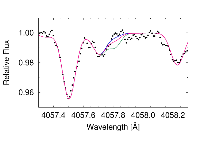
Figure 13: Same as Figure 7, but for the Pb I line at 4058 Å. Assumed abundances are $\log\epsilon(\mathrm{Pb})=-0.4$, $-0.1$, and $+0.2$. Note that, for values greater than $\log\epsilon(\mathrm{Pb})=-0.1$, our adopted uppper limit, Pb should clearly be detectable.

The upper limit on the Pb abundance, $\log\epsilon(\mathrm{Pb})<-0.10$, is estimated from a comparison of the observed spectrum with synthetic spectra in the region of the 4057.8 Å Pb I line (Figure 13). The line list for the Pb isotopes of Van Eck et al. (2003) is adopted, and Solar System Pb isotope ratios are assumed. In the spectrum synthesis, we modified the C and Mg abundances, within their errors, so as to fit the CH and Mg lines neighboring the Pb I line.

5 Discussion

5.1 Origin of the Carbon Excess

As shown by previous studies, CEMP-no stars are intriguing objects. They tend to have lower metallicity than CEMP-s and most carbon-normal stars, and are thus expected to offer vital clues for understanding the chemical evolution of the early Universe. However, consensus on the nucleosynthetic origin of this class of stars has yet to be reached. BD+44^∘493 is a particularly important star for addressing this question, as it is by far the brightest CEMP-no star at extremely low metallicity. In this section, we examine the scenarios that have been proposed to account for the origin of CEMP-no stars, by comparing the obtained abundance pattern of BD+44^∘493 with theoretical predictions.

We first note that self-enrichment of carbon by dredge-up of the products of the helium burning (e.g., Fujimoto et al. 2000) is clearly excluded, because BD+44^∘493 is an unevolved subgiant.

Mass transfer from a companion AGB star is proposed as one of the causes of C enrichment for many CEMP stars, and such a model has had great success in explaining the observed properties of CEMP-s stars (e.g. Käppeler et al., 2011). However, the observed properties of BD+44^∘493 do not support this scenario. The first difficulty, which applies to all CEMP-no stars (by definition), is that the neutron-capture elements that are expected to be enhanced by an AGB companion are not over-abundant in this star. Cohen et al. (2006), following Busso et al. (1999), suggested that the apparently normal Ba abundances of CEMP-no stars might be explained by the high neutron-to- Fe-peak-element seed ratio in the s-process that occurred in the AGB companion, resulting in little or no Ba excess, but large Pb enhancement. This follows, according to Busso et al. (1999), because the very large number of neutrons available per Fe-peak-element seed nucleus at low metallicity forces the $s$-process to run to completion, and terminate on lead. Under this hypothesis, the Pb abundance predicted by Cohen et al. (2006) is $\log\epsilon(\mathrm{Pb})=1.5$ at [Fe/H] $=-3.5$, although they comment that its detection would be difficult, because of the weakness of the line, and its location in a spectral region contaminated by a “thicket of CH features.” In this regard, we are fortunate that BD+44^∘493 is as bright as it is, since the high S/N spectrum we have obtained (as well as the relatively high effective temperature) provides the opportunity to set a meaningful upper limit, even from measurements in the optical. Our measured upper limit for lead in BD+44^∘493, ($\log\epsilon(\mathrm{Pb})<-0.10$), is clearly much lower than the predicted value from Cohen et al. (2006), $\log\epsilon(\mathrm{Pb})=1.5$.

Komiya et al. (2007) discussed the possibility that, since a relatively high-mass companion AGB star ($M>3.5M_{\odot}$) produces little s-process elements, due to inefficient radiative ¹³C burning, this might account for the lack of Ba enrichment in CEMP-no stars. However, since a high-mass AGB star converts C into N via hot-bottom burning, the low N abundance of BD+44^∘493 permits only a narrow range of mass. Another constraint is the low C/O ratio (C/O $<1$) found for BD+44^∘493, which cannot be explained by the AGB nucleosynthesis scenario (e.g., Nishimura et al., 2009). Moreover, the radial velocity of BD+44^∘493 has stayed constant since 1984 (§2.3), indicating no signature of binarity (or only allowing a binary of very long period). Our conclusion is that the binary mass-transfer scenario is excluded as the origin of the C excess of BD+44^∘493.

Another scenario that has been put forward, that the C enhancement occurs prior to the formation of (at least some) CEMP stars due to the predicted mass loss from rapidly-rotating massive stars of the lowest metallicity. Meynet et al. (2006) explored models of rapidly-rotating $60M_{\odot}$ stars with total metallicities $Z=10^{-8}$ and $10^{-5}$, and found that strong internal mixing increases the total metallicity at the stellar surface significantly, leading to large mass loss in the form of a vigorous wind. The ejecta are highly enriched in CNO elements, which are products of triple-$\alpha$ reactions and the CNO cycle. In particular, the N excess is predicted to be quite large, due to operation of the CNO cycle in the H-burning shell, which converts C into N. The low observed N abundance of BD+44^∘493, however, cannot be accounted for by this scenario. Furthermore, recent models of rotating massive stars with $Z=0$ explored by Ekström et al. (2008), over a wide range of mass (9 - 200$M_{\odot}$), suggest that these stars experience only relatively little mass loss, in stark contrast to that from extremely low, but non-zero, metallicity models. Their results indicate that the very first generation of stars, even though they might be rapidly rotating, are unlikely to lead to CNO enrichment through mass loss.

A remaining possibility is element production by so-called faint supernovae associated with the first generations of stars, which experience extensive mixing of matter and fallback onto the nascent compact object that forms at their centers during their explosions (Umeda & Nomoto, 2003, 2005; Tominaga et al., 2007b). Such a process is apparently realized in relativistic jet-induced supernovae with low energy-deposition rates (Tominaga et al., 2007a). Since a relatively large amount of material collapses onto the central remnant in such supernovae, only small amounts of heavy elements, such as the Fe-peak elements (which are synthesized in the inner regions of the progenitors) can be ejected, compared to lighter elements, such as C, which are synthesized in the outer regions. Thus, high [C/Fe] and [O/Fe] ratios are predicted in the ejected material. Since the luminosity of supernovae is generated by the radioactive decay of ⁵⁶Ni through ⁵⁶Co to ⁵⁶Fe, the small amount of ⁵⁶Ni ejected results in the faintness of the explosion.

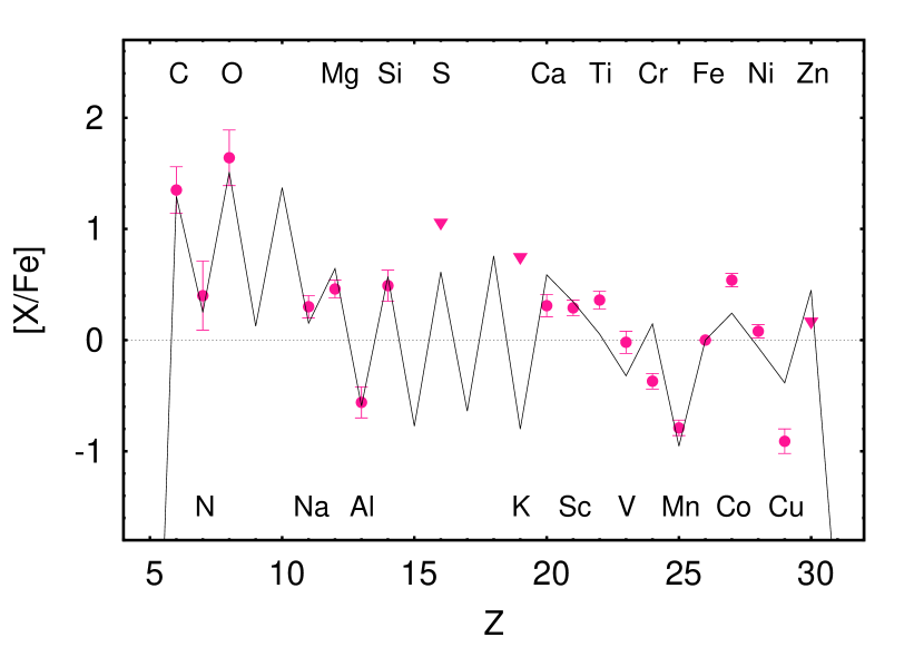
Figure 14: Comparison between the observed elemental abundance pattern of BD+44^∘493 (filled circles) and the theoretical individual supernova yields (solid lines). The upper limits on the abundances for several elements by the observation are shown by triangles. See text for details of the supernova model.

This scenario does not produce a serious conflict with the observed elemental-abundance pattern of BD+44^∘493. Indeed, a faint Pop III supernova model which undergo mixing-and-fallback during the explosion can well-reproduce the abundance pattern of this object, as shown in Figure 14. This model is constructed with the same method as in Tominaga et al. (2007b) for a main-sequence mass of 25Msun (Umeda & Nomoto, 2005), and explosion energy of $5\times 10^{51}$ ergs, while a normal supernova explodes with an energy of $\sim 1\times 10^{51}$ ergs; the ejected ⁵⁶Ni mass is only about 10% of that for a normal supernova. Since a supernova with high entropy leads to a large [Zn/Fe] ratio (Umeda & Nomoto, 2005; Tominaga et al., 2007b), our low upper limit for [Zn/Fe] for BD+44^∘493 may constrain the explosion energy, and favor a supernova with normal entropy. The low [N/C] in BD+44^∘493 indicates that mixing between the He convective shell and H-rich envelope during pre-supernova evolution is not significant (Iwamoto et al., 2005), and in the calculation only 15% of the C in the He layer is assumed to be converted into N, in order to reproduce the abundance pattern. Thus, at present, a faint supernova is the most promising candidate for the origin of the C excess in BD+44^∘493.

Our conclusion on the origin of the C excess in BD+44^∘493 impacts the interpretation of the entire CEMP-no class of stars. Faint supernovae should have played an important role in the chemical evolution of the early Galaxy, and at least some (perhaps all) CEMP-no stars probably formed from gas polluted by them. This supports the notion that the ultra metal-poor (UMP; [Fe/H] $<-4.0$) and hyper metal-poor stars (HMP; [Fe/H] $<-5.0$) are not low-mass Pop III stars but, rather, Pop II stars that formed from gas that had been pre-enriched by high-mass Pop III stars.

Norris et al. (2012) discussed the possible existence of two cooling channels responsible for the formation of second-generation stars from gas clouds polluted by first generations of massive stars, following the studies by Bromm & Loeb (2003) and Frebel et al. (2007a). One of them is the process responsible for non carbon-enhanced stars, which is not yet well-defined; dust-induced cooling is a candidate. The other is the cooling by fine-structure lines of C II and O I in the case of carbon and oxygen-enhanced material. Our conclusion that BD+44^∘493 is formed from a gas cloud pre-enriched in carbon supports the existence of this channel of EMP star formation.

5.2 Production and Depletion of Light Elements

Figure 15 shows the Be abundance upper limit for BD+44^∘493 in the $\log\epsilon(\mathrm{Be})$ vs. [Fe/H] plane, along with the results from Rich & Boesgaard (2009). Our observation (an upper limit) is consistent with the linear trend between Be and Fe seen in this figure. It is of significance that the Be abundance keeps decreasing and exhibits no plateau at low metallicity, at least to the level of $\log\epsilon(\mathrm{Be})<-1.8$. Previous measurements of Be for stars permitted the possibility of a Be plateau around $\log\epsilon(\mathrm{Be})\sim-1.4$ (Primas et al., 2000a, b), which would now be clearly called into question.

Our analysis is the first attempt to measure a Be abundance for a CEMP star. Since Be is produced via the spallation of CNO nuclei, CNO abundances, especially O abundances, have been expected to correlate with Be abundances. However, our low Be upper limit shows that the high C and O abundances in BD+44^∘493 are irrelevant to its Be abundance (Figure 15, lower panel). Moreover, the origin of the C excess in CEMP-no stars such as BD+44^∘493, which we have argued is most likely due to faint supernovae, is unlikely to be a significant source of high-energy CNO nuclei that participate in the primary spallation process expected to be associated with Be production.

Be abundances, as well the abundances of B, in metal-poor stars are proposed to be good indicators of the ages of stars formed in the early Galaxy (Suzuki et al., 1999; Beers et al., 2000; Smiljanic et al., 2010), because they could reflect the increase of cosmic ray flux in the early Galaxy, while other metals such as Fe would reflect the contributions from individual supernovae, and result in a spatial inhomogeneity in the abundance ratios. Our finding that Be is not significantly enhanced even by the supernovae that yield large amounts of C and O, provides additional support for this hypothesis.

The above discussion is, however, based on the assumption that the Be abundance in BD+44^∘493 is not depleted during its evolution. Beryllium is a fragile element, with a burning temperature of $\sim 3.0\times 10^{6}\,\mathrm{K}$, higher than that of Li ($2.5\times 10^{6}\,\mathrm{K}$). Given that the Li abundance of this star, $\log\epsilon(\mathrm{Li})=1.0$, is much lower than the Spite plateau value, we should also examine the possibility of Be depletion in BD+44^∘493.

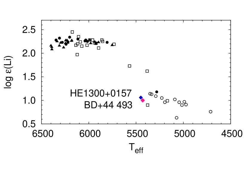
Figure 16: Li abundances for metal-poor ($\mathrm{[Fe/H]}<-1.4$) dwarfs and subgiants, as a function of effective temperature. Our result for BD+44^∘493 is shown by the (pink) diamond, whereas the (blue) diamond indicates HE 1300+0157 (Frebel et al., 2007b). Open circles represent the results of García Pérez et al. (2006). Open squares, filled circles, and filled triangles were taken from Boesgaard & Novicki (2006), Shi et al. (2007), and Asplund et al. (2006), respectively. For $T_{\mathrm{eff}}<5700\,\mathrm{K}$, only subgiants ($\log g<4.0$) are plotted.

In Figure 16, we compare the Li abundance of BD+44^∘493 with those of other metal-poor ($\mathrm{[Fe/H]}<-1.4$) subgiants, which are mainly taken from García Pérez et al. (2006), as well as metal-poor dwarfs with $T_{\mathrm{eff}}>5700\,\mathrm{K}$. As a star evolves from the main sequence to the red giant branch, the effective temperature decreases, that is, cooler subgiants in this diagram are more evolved. At $T_{\mathrm{eff}}>5700\,\mathrm{K}$, metal-poor subgiants appear to have Li abundances consistent with the Spite plateau values, along with the metal-poor dwarfs. The sharp decline of Li abundances in the range 5700 - 5400 K indicates that significant Li depletion occurs when stars pass through this temperature range, often referred to as the Boesgaard dip (Boesgaard & King, 2002). García Pérez et al. (2006) concluded that their subgiants have depleted Li abundances that are generally consistent with predictions from standard models of stellar evolution (Deliyannis et al., 1990). Since the Li abundance of BD+44^∘493 is in agreement with the values found for their sample, we conclude that the Li depletion in BD+44^∘493 is likely to be similar to those found in their sample, even though the metallicity is remarkably lower.

In order to investigate Be depletion, we adopt [Be/Fe] as an indicator. We assume that metal-poor stars originally have Be abundances in proportion to their Fe abundances, as found in Figure 15, that is, [Be/Fe] is close to 0.2. If Be is not depleted in a subgiant, the star is expected to follow the linear correlation, and have the same [Be/Fe] value as dwarfs, while lower [Be/Fe] values suggest Be depletion in the star. In Figure 17, we plot [Be/Fe] versus effective temperature for metal-poor subgiants ($\mathrm{[Fe/H]}<-1.4$; the same metallicity range as adopted for discussion on Li depletion). It appears that objects with $T_{\mathrm{eff}}>5700\,\mathrm{K}$ did not experience Be depletion, as expected from our discussion on the Li abundances in the temperature range. On the other hand, [Be/Fe] values in cool subgiants are about one order of magnitude lower, which could be interpreted as the result of Be depletion.

During the subgiant phase, the stellar convection zone extends into the interior, first reaching to the Li-depleted layer, and later, to the Be-depleted layer, because nuclear Be burning requires higher temperatures than Li burning. Therefore, Be depletion is expected in more-evolved subgiants with lower effective temperatures than Li depletion. However, this is not clearly found in Figures 16 and 17. One reason might be the paucity of stars of the sample in the temperature range 5400 - 5700 K. More measurements of Li and Be abundances for metal-poor subgiants in this temperature range are strongly desired in order to assess this issue. Futhermore, the uncertainty in effective temperature determinations could make the difference unclear. In comparisons with the results of previous studies, consistency of temperature determinations are essential. Since BD+44^∘493 has an effective temperature of 5430 K that falls into the range where Be depletion appears to occur, it is difficult to conclude whether or not Be is depleted in this star.

Another constraint on Be depletion could be obtained from boron abundance measurements. If B is depleted in a star, Be also must be depleted, because the burning temperature of B, $5.0\times 10^{6}\,\mathrm{K}$, is higher than that of Be. The absence of an available B line in the wavelength range that can be accessed from ground-based telescopes makes a B abundance measurement a challenge. The STIS (Space Telescope Imaging Spectrograph) instrument onboard the Hubble Space Telescope is at present the only spectrograph with which we could observe the B II resonance lines at 2497 Å. Abundance measurements of Li, Be, and B for metal-poor subgiants will offer important clues for our understanding of mixing processes in stellar interiors, which can decrease surface abundances of light elements. Theoretical modeling of the depletion for a wide range of metallicity and stellar mass should also be explored.

6 Summary and Concluding Remarks

We have conducted a detailed elemental abundance analysis for the 9th magnitude EMP star BD+44^∘493, based on very high-quality, high-resolution optical and near-UV spectra. This object is a CEMP-no star, and has exhibited no detectable radial-velocity variations over the past 24 years. The abundance patterns we measure, in particular C, N, O, as well as the heavy neutron-capture elements, suggest that the most likely origin of this object is that it was born from gas polluted by the elements produced by a faint supernova undergoing mixing and fallback, which ejected only a small amount of metals beyond C, N, and O.

Recent searches for EMP stars have revealed that the fraction of CEMP stars among them is substantially higher than that for less metal-poor stars (Carollo et al., 2012), and that CEMP-no stars are an important contributor to these (e.g., Aoki et al., 2012; Norris et al., 2012). The HMP stars HE 1327–2326 and HE 0107–5240 are included in this class of objects. The results for BD+44^∘493 suggest a very important role for faint supernovae in the earliest phase of chemical enrichment in the Galaxy, and (at least for some low-mass stars) the importance of cooling by fine-structure lines of C II and O I in their early formation.

The low observed Li abundance and non-detection of Be for BD+44^∘493 also shed new light on the production of light elements in the early Galaxy. However, it remains possible that these elements could have been depleted in this star during the course of its evolution. A future (space-based) measurement of B for this star has particular importance to distinguish whether these effects apply or not. Further measurements of Li and Be for subgiants with $T_{\mathrm{eff}}$ of about 5500 K, in which depletion of these elements first appears, are also useful for understanding the nature of light elements in EMP stars.

Finally, we emphasize that our measured upper limit on the abundance of Pb ($\log\epsilon$(Pb)$<-0.10$) rejects that possibility that the observed neutron-capture-element abundance patterns in BD+44^∘493 arise from the operation of a modified $s$-process at low metallicity in CEMP-no stars. High-resolution spectroscopy in the region of the UV Pb line of BD+44^∘493 from HST/STIS has recently been obtained by Beers et al. (in preparation), and can be used to confirm our estimated limit. Taken at face value, our present result already provides additional strong evidence that the C and O enhancements in BD+44^∘493 must have originated in an astrophysical site other than AGB stars, as discussed in §5.1. Additional measurements of Pb from the ground and with HST/STIS would be highly desirable to obtain for low-metallicity CEMP-no stars, if other sufficiently bright examples are identified in the future.

W.A. and N.T. were supported by the JSPS Grants-in-Aid for Scientific Research (23224004). T.C.B. acknowledges partial funding of this work from grants PHY 02-16783 and PHY 08-22648: Physics Frontier Center/Joint Institute for Nuclear Astrophysics (JINA), awarded by the U.S. National Science Foundation.

Facilities: Subaru (HDS)

Appendix A A spectral atlas of BD+44^∘493

BD+44^∘493 is, by far, the brightest object among EMP stars found to date. As such, the very high-quality spectrum of this star analyzed in the present work can serve as a useful template for future studies of EMP and CEMP stars. Since this object is a CEMP-no star, it displays clear excesses of C and O, and is at an effective temperature ($T_{\mathrm{eff}}$ = 5430 K) such that many CH and OH features are identifiable in the near-UV and blue spectral regions.

We provide an atlas of the spectrum of BD+44^∘493 as online-only figures. Figure 18 shows a portion of the atlas. The full spectrum covers the wavelength range from 3080 Å to 9370 Å. A small portion of this wavelength region is not covered, due to the gap in the two CCDs in HDS (5330–5430 Å), and in the redder regions where the limited size of the CCDs does not fully cover the free spectral range ($>7000$ Å), as well as due to the occasional bad columns of the CCDs. Some spectral regions are affected by telluric absorption that is not fully corrected. The wavelength range between 3900–3960 Å is not covered by the spectrum obtained with resolving power of $R=90,000$, but it is supplemented by the $R=60,000$ spectrum (see § 2).

The atomic lines used in the abundance analysis in the present work are indicated by the shorter (red) lines extended down from the top of each panel. Other atomic lines that were not used in the analysis, including hydrogen lines, are shown by the longer (blue) lines. Molecular features used in this analysis are shown by lines extending up from the bottom of each panel for OH (long, blue), CH (short, red) and NH (middle, green).

Figure 1: Heliocentric radial velocity of BD+44^∘493 from 1984 to 2008. Our measurements are represented by the filled circles. The open circles indicate the results of Carney et al. (2003). The solid line indicates the mean of the entire sample ($-150.66$ km s^-1) and the dashed lines show the rms variation (0.73 km s^-1).

Figure 2: Stellar and interstellar Na I D lines in the spectrum of BD+44^∘493.

Figure 4: Adopted surface gravity and effective temperature for BD+44^∘493, with error bars indicating their uncertainties, in comparison with Yonsei-Yale (Kim et al., 2002; Demarque et al., 2004) isochrones with $\mathrm{[Fe/H]}=-3.5$ and $\mathrm{[\alpha/Fe]}=+0.3$ for 11 Gyr (left), 12 Gyr (middle) and 13 Gyr (right).

.

Figure 6: Fe abundances determined from individual Fe I and Fe II lines, as a function of wavelength. The open circles and filled diamonds represent Fe I and Fe II lines, respectively.

Figure 15: Be abundances, as a function of [Fe/H] (upper panel) and [O/H] (lower panel). The upper limit for BD+44^∘493 is shown by the filled triangle. Filled circles represent the result of Rich & Boesgaard (2009).

Figure 17: [Be/Fe] ratios, as a function of effective temperature for metal-poor ($\mathrm{[Fe/H]}<-1.4$) subgiants ($\log g<4.0$). Our upper limit for BD+44^∘493 is shown by the pink triangle. Open symbols indicate the results of García Pérez et al. (2006). Filled symbols were taken from Rich & Boesgaard (2009), Smiljanic et al. (2009), and Tan et al. (2009). All triangles mean upper limits.

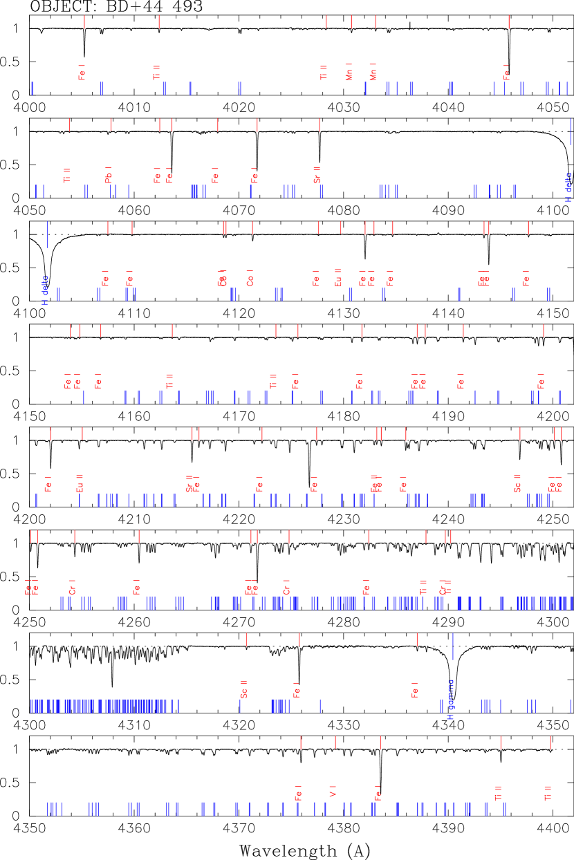
Figure 18: A portion of the spectral atlas of BD+44^∘493. The full set of plots are provided online only.

Table 1: Subaru/HDS Observations of BD+44^∘493 and HD 12534

Target	Universal Time	Wavelength	Resolving	CCD Binning	Total Time
		(Å)	Power	(pixels)	(sec)
BD+44∘493	2008 Aug 22, 15:19	4030–5330, 5430–6730	60,000	$2\times 2$	600
BD+44∘493	2008 Oct 4, 09:00	4030–5330, 5430–6770	90,000	$1\times 1$	1200
BD+44∘493	2008 Oct 4, 09:28	6690–7960, 8080–9370	90,000	$1\times 1$	1500
BD+44∘493	2008 Oct 5, 10:06	3080–3900, 3960–4780	90,000	$1\times 1$	7200
BD+44∘493	2008 Nov 16, 05:37	3540–4350, 4420–5240	60,000	$2\times 2$	300
HD12534	2008 Oct 4, 08:53	4030–5330, 5430–6770	90,000	$1\times 1$	90
HD12534	2008 Oct 4, 09:57	6690–7960, 8080–9370	90,000	$1\times 1$	150
HD12534	2008 Oct 5, 09:58	3080–3900, 3960–4780	90,000	$1\times 1$	135

Table 2: Line Data and Equivalent Widths

Species	Wavelength	$\log gf$	l.e.p.	$W$	Remarks
	Å		(eV)	mÅ
Na I	5889.951	0.117	0.000	66.03
Na I	5895.924	-0.184	0.000	45.26
Mg I	3829.355	-0.208	2.707	92.04
Mg I	3832.304	0.270	2.710	113.44
Mg I	3838.292	0.490	2.715	125.23
Mg I	4571.096	-5.393	0.000	3.17
Mg I	4702.991	-0.380	4.330	12.65
Mg I	5172.684	-0.450	2.712	97.88
Mg I	5183.604	-0.239	2.717	111.01
Mg I	5528.405	-0.341	4.346	11.56
Al I	3961.529	-0.336	0.014	42.38
Si I	3905.522	-1.090	1.909	82.35
Si I	3905.522	-1.090	1.909	82.35
Si I	3905.522	-1.090	1.909	82.35
V II	3545.190	-0.390	1.100	1.76
V II	3592.030	-0.370	1.100	1.69
Ti I	3653.490	0.220	0.050	7.58
Ti I	3989.759	-0.140	0.021	3.49
Ti I	3998.636	0.000	0.048	5.24
Ti I	4533.249	0.530	0.848	2.97
Ti I	4534.776	0.340	0.836	1.90
Ti I	4981.731	0.560	0.848	3.31
Ti I	5007.210	0.168	0.818	2.28
Ti II	3148.050	-1.200	0.000	37.23
Ti II	3190.880	0.190	1.080	38.18
Ti II	3222.840	-0.480	0.010	66.56
Ti II	3229.200	-0.550	0.000	68.46
Ti II	3236.580	0.230	0.030	82.99
Ti II	3239.040	0.060	0.010	78.88
Ti II	3241.990	-0.050	0.000	75.44
Ti II	3261.620	0.080	1.230	33.28
Ti II	3278.290	-0.210	1.230	15.53
Ti II	3282.320	-0.290	1.220	12.46
Ti II	3287.660	0.340	1.890	15.09
Ti II	3302.110	-2.330	0.150	4.89
Ti II	3321.700	-0.320	1.230	14.52
Ti II	3322.940	-0.090	0.150	70.79
Ti II	3326.780	-1.180	0.110	34.93
Ti II	3329.450	-0.270	0.140	65.21
Ti II	3332.110	-0.150	1.240	45.49
Ti II	3335.200	-0.440	0.120	60.23
Ti II	3340.360	-0.610	0.110	57.25
Ti II	3343.760	-1.270	0.150	31.66
Ti II	3349.040	0.470	0.610	68.20
Ti II	3361.220	0.280	0.030	94.82
Ti II	3372.800	0.270	0.010	88.52
Ti II	3380.280	-0.570	0.050	63.88
Ti II	3383.770	0.140	0.000	86.13
Ti II	3387.850	-0.430	0.030	66.91
Ti II	3394.580	-0.540	0.010	63.60
Ti II	3456.390	-0.230	2.060	3.15
Ti II	3477.190	-0.970	0.120	44.47
Ti II	3489.740	-1.920	0.140	8.43
Ti II	3491.070	-1.060	0.110	39.03
Ti II	3573.730	-1.500	0.570	7.35
Ti II	3641.330	-0.710	1.240	11.77
Ti II	3685.190	-0.040	0.570	72.47
Ti II	3814.580	-1.700	0.570	11.79
Ti II	3900.551	-0.280	1.130	24.96
Ti II	3913.468	-0.410	1.120	21.83
Ti II	4012.390	-1.610	0.570	6.19
Ti II	4028.343	-0.990	1.892	2.34
Ti II	4053.834	-1.060	1.893	1.18
Ti II	4163.648	-0.210	2.590	1.43
Ti II	4173.537	-1.815	1.084	2.43
Ti II	4287.872	-1.820	1.080	1.64
Ti II	4290.219	-0.930	1.165	7.85
Ti II	4395.033	-0.460	1.084	20.93
Ti II	4399.772	-1.220	1.237	7.42
Ti II	4417.719	-1.190	1.165	4.17
Ti II	4443.794	-0.720	1.080	15.75
Ti II	4464.450	-1.810	1.161	1.58
Ti II	4468.507	-0.600	1.131	15.40
Ti II	4501.273	-0.770	1.116	13.24
Ti II	4533.969	-0.540	1.237	13.03
Ti II	4563.761	-0.690	1.221	9.44
Ti II	4571.968	-0.320	1.572	10.62
Ti II	4589.958	-1.620	1.237	1.49
Sc II	3353.720	0.250	0.310	20.00
Sc II	3535.710	-0.470	0.310	5.89
Sc II	3572.526	0.267	0.022	46.07
Sc II	3576.340	0.007	0.008	26.50
Sc II	3580.925	-0.149	0.000	21.27
Sc II	3590.470	-0.550	0.020	9.56
Sc II	3630.740	0.220	0.010	35.69
Sc II	3645.310	-0.420	0.020	13.53
Sc II	4246.837	0.240	0.315	29.66
Sc II	4320.732	-0.252	0.605	5.00
Sc II	4400.399	-0.540	0.605	3.39
Sc II	4415.563	-0.670	0.595	2.13
Cr I	3593.480	0.310	0.000	29.60
Cr I	4254.332	-0.114	0.000	21.27
Cr I	4274.796	-0.231	0.000	19.32
Cr I	4289.716	-0.361	0.000	16.35
Cr I	5206.038	0.019	0.941	5.97
Cr I	5208.419	0.158	0.941	7.49
Cr II	3118.650	-0.100	2.420	23.35
Cr II	3408.760	-0.040	2.480	14.41
Mn I	4030.763	-0.470	0.000	7.11
Mn I	4033.060	-0.618	0.000	4.30
Mn II	3441.990	-0.273	1.780	11.45
Mn II	3460.320	-0.540	1.810	5.93
Mn II	3488.680	-0.860	1.850	2.25
Fe I	3225.790	0.380	2.400	27.36
Fe I	3286.750	-0.170	2.180	21.74
Fe I	3407.460	-0.020	2.180	26.08
Fe I	3440.610	-0.670	0.000	92.40
Fe I	3440.990	-0.960	0.050	82.79
Fe I	3443.880	-1.370	0.090	69.59
Fe I	3475.450	-1.050	0.090	79.44
Fe I	3476.700	-1.510	0.120	63.99
Fe I	3490.570	-1.110	0.050	78.85
Fe I	3497.840	-1.550	0.110	63.13
Fe I	3521.260	-0.990	0.920	47.91
Fe I	3536.560	0.120	2.880	9.38
Fe I	3554.930	0.540	2.830	20.21
Fe I	3558.510	-0.630	0.990	60.21
Fe I	3565.380	-0.130	0.960	73.34
Fe I	3570.100	0.150	0.920	91.51
Fe I	3581.190	0.410	0.860	96.92
Fe I	3585.320	-0.800	0.960	54.52
Fe I	3585.710	-1.190	0.920	42.65
Fe I	3586.110	0.170	3.240	6.64
Fe I	3586.990	-0.800	0.990	52.90
Fe I	3603.200	-0.260	2.690	7.28
Fe I	3608.860	-0.100	1.010	74.12
Fe I	3618.770	0.000	0.990	76.59
Fe I	3621.460	-0.020	2.730	10.91
Fe I	3622.000	-0.150	2.760	7.53
Fe I	3631.460	-0.040	0.960	80.98
Fe I	3640.390	-0.110	2.730	8.22
Fe I	3647.840	-0.190	0.920	77.55
Fe I	3727.619	-0.620	0.958	65.02
Fe I	3743.362	-0.780	0.990	59.53
Fe I	3745.561	-0.770	0.087	97.81
Fe I	3745.900	-1.340	0.121	78.13
Fe I	3758.233	-0.020	0.958	83.49
Fe I	3763.789	-0.230	0.990	75.98
Fe I	3767.192	-0.389	1.011	69.21
Fe I	3786.680	-2.220	1.010	7.82
Fe I	3787.880	-0.859	1.011	55.84
Fe I	3790.093	-1.740	0.990	20.28
Fe I	3812.964	-1.030	0.958	51.49
Fe I	3815.840	0.240	1.485	74.11
Fe I	3820.425	0.140	0.859	97.49
Fe I	3824.444	-1.362	0.000	85.00
Fe I	3825.881	-0.030	0.915	87.53
Fe I	3827.823	0.080	1.557	64.94
Fe I	3840.440	-0.510	0.990	68.58
Fe I	3841.048	-0.045	1.608	57.20
Fe I	3843.260	-0.240	3.050	5.11
Fe I	3849.967	-0.870	1.011	55.15
Fe I	3850.818	-1.740	0.990	19.68
Fe I	3856.372	-1.280	0.052	83.81
Fe I	3859.911	-0.710	0.000	104.34
Fe I	3865.523	-0.950	1.011	52.93
Fe I	3878.018	-0.896	0.958	58.79
Fe I	3878.573	-1.360	0.087	83.55
Fe I	3895.656	-1.660	0.110	71.42
Fe I	3899.707	-1.520	0.087	76.59
Fe I	3902.946	-0.440	1.558	47.77
Fe I	3906.480	-2.200	0.110	44.76
Fe I	3917.180	-2.150	0.990	8.69
Fe I	3920.258	-1.740	0.121	66.89
Fe I	3922.912	-1.640	0.052	74.87
Fe I	3927.920	-1.522	0.110	77.97
Fe I	3930.297	-1.491	0.087	77.30
Fe I	3956.680	-0.430	2.690	7.27
Fe I	3225.790	0.380	2.400	27.36
Fe I	3286.750	-0.170	2.180	21.74
Fe I	3407.460	-0.020	2.180	26.08
Fe I	3440.610	-0.670	0.000	92.40
Fe I	3440.990	-0.960	0.050	82.79
Fe I	3443.880	-1.370	0.090	69.59
Fe I	3475.450	-1.050	0.090	79.44
Fe I	3476.700	-1.510	0.120	63.99
Fe I	3490.570	-1.110	0.050	78.85
Fe I	3497.840	-1.550	0.110	63.13
Fe I	3521.260	-0.990	0.920	47.91
Fe I	3536.560	0.120	2.880	9.38
Fe I	3554.930	0.540	2.830	20.21
Fe I	3558.510	-0.630	0.990	60.21
Fe I	3565.380	-0.130	0.960	73.34
Fe I	3570.100	0.150	0.920	91.51
Fe I	3581.190	0.410	0.860	96.92
Fe I	3585.320	-0.800	0.960	54.52
Fe I	3585.710	-1.190	0.920	42.65
Fe I	3586.110	0.170	3.240	6.64
Fe I	3586.990	-0.800	0.990	52.90
Fe I	3603.200	-0.260	2.690	7.28
Fe I	3608.860	-0.100	1.010	74.12
Fe I	3618.770	0.000	0.990	76.59
Fe I	3621.460	-0.020	2.730	10.91
Fe I	3622.000	-0.150	2.760	7.53
Fe I	3631.460	-0.040	0.960	80.98
Fe I	3640.390	-0.110	2.730	8.22
Fe I	3647.840	-0.190	0.920	77.55
Fe I	3727.619	-0.620	0.958	65.02
Fe I	3743.362	-0.780	0.990	59.53
Fe I	3745.561	-0.770	0.087	97.81
Fe I	3745.900	-1.340	0.121	78.13
Fe I	3758.233	-0.020	0.958	83.49
Fe I	3763.789	-0.230	0.990	75.98
Fe I	3767.192	-0.389	1.011	69.21
Fe I	3786.680	-2.220	1.010	7.82
Fe I	3787.880	-0.859	1.011	55.84
Fe I	3790.093	-1.740	0.990	20.28
Fe I	3812.964	-1.030	0.958	51.49
Fe I	3815.840	0.240	1.485	74.11
Fe I	3820.425	0.140	0.859	97.49
Fe I	3824.444	-1.362	0.000	85.00
Fe I	3825.881	-0.030	0.915	87.53
Fe I	3827.823	0.080	1.557	64.94
Fe I	3840.440	-0.510	0.990	68.58
Fe I	3841.048	-0.045	1.608	57.20
Fe I	3843.260	-0.240	3.050	5.11
Fe I	3849.967	-0.870	1.011	55.15
Fe I	3850.818	-1.740	0.990	19.68
Fe I	3856.372	-1.280	0.052	83.81
Fe I	3859.911	-0.710	0.000	104.34
Fe I	3865.523	-0.950	1.011	52.93
Fe I	3878.018	-0.896	0.958	58.79
Fe I	3878.573	-1.360	0.087	83.55
Fe I	3895.656	-1.660	0.110	71.42
Fe I	3899.707	-1.520	0.087	76.59
Fe I	3902.946	-0.440	1.558	47.77
Fe I	3906.480	-2.200	0.110	44.76
Fe I	3917.180	-2.150	0.990	8.69
Fe I	3920.258	-1.740	0.121	66.89
Fe I	3922.912	-1.640	0.052	74.87
Fe I	3927.920	-1.522	0.110	77.97
Fe I	3930.297	-1.491	0.087	77.30
Fe I	3956.680	-0.430	2.690	7.27
Fe I	4005.242	-0.600	1.558	42.04
Fe I	4045.812	0.280	1.486	78.17
Fe I	4062.441	-0.862	2.845	1.84
Fe I	4063.594	0.062	1.558	67.63
Fe I	4067.978	-0.472	3.211	2.13
Fe I	4071.738	-0.008	1.608	62.82
Fe I	4107.488	-0.879	2.831	1.62
Fe I	4109.802	-0.895	2.845	1.77
Fe I	4118.545	0.215	3.573	4.34
Fe I	4127.608	-0.990	2.858	1.55
Fe I	4132.058	-0.675	1.608	37.12
Fe I	4132.899	-1.006	2.845	1.99
Fe I	4134.678	-0.649	2.831	3.32
Fe I	4143.415	-0.204	3.047	5.36
Fe I	4143.868	-0.511	1.558	45.70
Fe I	4147.669	-2.090	1.485	3.80
Fe I	4153.900	-0.321	3.396	2.30
Fe I	4154.806	-0.400	3.368	2.02
Fe I	4156.799	-0.809	2.831	2.61
Fe I	4175.636	-0.827	2.845	2.42
Fe I	4181.755	-0.371	2.831	6.91
Fe I	4187.039	-0.541	2.449	10.20
Fe I	4187.795	-0.530	2.425	11.44
Fe I	4191.431	-0.666	2.469	6.81
Fe I	4199.095	0.156	3.047	13.61
Fe I	4202.029	-0.689	1.485	43.19
Fe I	4216.184	-3.356	0.000	10.84
Fe I	4222.213	-0.914	2.449	4.35
Fe I	4227.427	0.266	3.332	7.50
Fe I	4233.603	-0.579	2.482	8.14
Fe I	4235.937	-0.330	2.425	17.42
Fe I	4250.120	-0.380	2.469	12.69
Fe I	4250.787	-0.713	1.558	37.95
Fe I	4260.474	0.077	2.400	29.69
Fe I	4271.154	-0.337	2.449	18.47
Fe I	4271.761	-0.173	1.485	65.76
Fe I	4282.403	-0.779	2.176	10.50
Fe I	4325.762	0.006	1.608	65.23
Fe I	4337.046	-1.695	1.557	7.94
Fe I	4375.930	-3.020	0.000	20.68
Fe I	4383.545	0.208	1.485	80.38
Fe I	4404.750	-0.147	1.557	62.82
Fe I	4415.122	-0.621	1.608	43.25
Fe I	4427.310	-2.924	0.052	19.63
Fe I	4430.614	-1.728	2.223	1.47
Fe I	4447.717	-1.339	2.223	3.55
Fe I	4459.118	-1.310	2.176	4.42
Fe I	4461.653	-3.200	0.087	12.01
Fe I	4466.552	-0.600	2.831	3.95
Fe I	4476.019	-0.819	2.845	3.65
Fe I	4489.739	-3.930	0.121	2.18
Fe I	4494.563	-1.136	2.198	5.41
Fe I	4528.614	-0.850	2.176	10.66
Fe I	4531.148	-2.130	1.485	3.77
Fe I	4602.941	-2.209	1.485	3.35
Fe I	4871.318	-0.363	2.865	6.03
Fe I	4872.138	-0.567	2.882	4.27
Fe I	4891.492	-0.112	2.852	9.57
Fe I	4918.994	-0.342	2.845	5.79
Fe I	4920.503	0.068	2.832	14.19
Fe I	4957.299	-0.408	2.851	4.77
Fe I	4957.597	0.233	2.808	22.83
Fe I	4994.130	-3.080	0.915	2.41
Fe I	5006.119	-0.638	2.832	3.06
Fe I	5012.068	-2.642	0.859	7.31
Fe I	5041.756	-2.203	1.485	3.41
Fe I	5049.820	-1.420	2.279	2.90
Fe I	5051.635	-2.795	0.915	4.39
Fe I	5083.339	-2.958	0.958	2.94
Fe I	5123.720	-3.068	1.011	1.46
Fe I	5171.596	-1.793	1.485	9.71
Fe I	5191.455	-0.551	3.038	2.81
Fe I	5192.344	-0.421	2.998	3.66
Fe I	5216.274	-2.150	1.608	3.00
Fe I	5232.940	-0.058	2.940	9.05
Fe I	5266.555	-0.386	2.998	3.87
Fe I	5269.537	-1.321	0.860	59.09
Fe I	5270.356	-1.510	1.608	16.62
Fe I	5324.179	-0.240	3.211	4.85
Fe I	5328.039	-1.466	0.915	47.30
Fe I	5328.532	-1.850	1.557	6.76
Fe I	5429.697	-1.879	0.958	24.62
Fe I	5434.524	-2.122	1.011	14.20
Fe I	5446.917	-1.930	0.990	20.46
Fe I	5455.610	-2.091	1.011	16.05
Fe I	5497.516	-2.849	1.011	2.90
Fe I	5501.465	-2.950	0.958	2.06
Fe I	5506.779	-2.797	0.990	3.73
Fe I	5572.842	-0.310	3.396	1.80
Fe I	5586.756	-0.144	3.368	3.04
Fe I	5615.644	-0.140	3.332	4.57
Fe I	6136.615	-1.400	2.453	2.02
Fe I	6230.723	-1.281	2.559	2.02
Fe II	3255.900	-2.498	0.990	38.59
Fe II	3277.360	-2.191	0.990	44.91
Fe II	3281.300	-2.678	1.040	26.61
Fe II	3295.820	-2.900	1.080	15.13
Fe II	4233.172	-1.809	2.583	6.20
Fe II	4555.893	-2.250	2.828	1.39
Fe II	4583.837	-1.740	2.807	5.01
Fe II	4923.927	-1.206	2.891	10.61
Fe II	5018.430	-1.230	2.891	14.66
Fe II	5169.033	-1.140	2.891	20.04
Fe II	5316.615	-2.020	3.153	2.05
Co I	3409.170	-0.230	0.510	20.68
Co I	3412.330	0.030	0.510	31.92
Co I	3412.630	-0.780	0.000	31.99
Co I	3443.640	-0.010	0.510	29.51
Co I	3449.440	-0.500	0.430	17.63
Co I	3483.410	-1.000	0.510	4.42
Co I	3502.280	0.070	0.430	50.40
Co I	3502.620	-1.240	0.170	10.61
Co I	3518.350	0.070	1.050	8.81
Co I	3521.570	-0.580	0.430	11.95
Co I	3523.430	-0.440	0.630	16.97
Co I	3526.840	-0.620	0.000	47.06
Co I	3529.020	-0.880	0.170	17.13
Co I	3529.810	-0.070	0.510	31.89
Co I	3842.046	-0.770	0.923	3.79
Co I	3845.461	-0.010	0.923	15.66
Co I	3894.073	0.090	1.049	13.29
Co I	3995.302	-0.140	0.922	12.01
Co I	4118.767	-0.470	1.049	4.71
Co I	4121.311	-0.300	0.922	9.96
Ni I	3232.930	-1.010	0.000	51.74
Ni I	3243.050	-1.300	0.030	40.55
Ni I	3320.250	-1.420	0.170	29.03
Ni I	3369.560	-0.660	0.000	62.52
Ni I	3374.210	-1.760	0.030	23.48
Ni I	3391.040	-1.050	0.000	51.09
Ni I	3392.980	-0.540	0.030	63.76
Ni I	3413.930	-1.720	0.110	20.22
Ni I	3414.760	-0.029	0.025	78.42
Ni I	3423.711	-0.730	0.212	51.30
Ni I	3433.554	-0.683	0.025	61.42
Ni I	3437.270	-1.190	0.000	47.16
Ni I	3452.890	-0.910	0.109	51.28
Ni I	3461.650	-0.350	0.030	76.96
Ni I	3469.480	-1.820	0.280	12.34
Ni I	3472.540	-0.810	0.110	54.17
Ni I	3483.770	-1.110	0.280	37.16
Ni I	3492.950	-0.250	0.110	70.27
Ni I	3500.850	-1.280	0.170	36.24
Ni I	3519.760	-1.410	0.280	24.76
Ni I	3524.530	0.010	0.030	81.65
Ni I	3566.370	-0.240	0.420	56.40
Ni I	3571.860	-1.140	0.170	46.54
Ni I	3597.700	-1.100	0.210	41.83
Ni I	3610.461	-1.164	0.109	45.57
Ni I	3783.524	-1.304	0.423	23.63
Ni I	3807.138	-1.220	0.423	30.00
Ni I	3858.292	-0.951	0.423	42.03
Ni I	4714.408	0.260	3.380	1.11
Ni I	5476.900	-0.890	1.826	3.55
Cu I	3247.530	-0.060	0.000	17.76
Cu I	3273.950	-0.360	0.000	6.48
Sr II	4077.709	0.158	0.000	44.69
Sr II	4215.519	-0.155	0.000	32.39
Y II	3600.740	0.280	0.180	2.45
Zr II	3438.230	0.420	0.090	5.38
Zr II	3551.960	-0.310	0.090	1.38
Ba II	4554.029	0.163	0.000	5.35
Ba II	4934.076	-0.150	0.000	$<$3.18	Syn
Be II	3131.065	-0.468	0.000	$<$0.71	Syn
O I	6300.304	-9.819	0.000	$<$0.40	Syn
O I	7771.950	0.358	9.147	$<$2.00	Syn
K I	7698.974	-0.170	0.000	$<$2.00	Syn
V I	4379.230	0.550	0.301	$<$0.20	Syn
Zn I	3302.580	-0.057	4.030	$<$0.40	Syn
Zn I	3345.020	0.246	4.078	$<$0.40	Syn
Zn I	4722.153	-0.390	4.030	$<$0.20	Syn
Zn I	4810.528	-0.170	4.078	$<$0.50	Syn
Eu II	3819.670	0.510	0.000	$<$0.30	Syn
Eu II	4129.725	0.220	0.000	$<$0.20	Syn
Eu II	4205.040	0.210	0.000	$<$0.20	Syn
Pb I	4057.790	-0.200	1.320	$<$0.20	Syn

Table 3: Heliocentric Radial Velocities for BD+44^∘493

Epoch	HJD	$v_{\mathrm{helio}}$
		($\mathrm{km\,s^{-1}}$)
2008 Aug 22	2454701.14313	$-150.38$
2008 Oct 4	2454743.88522	$-149.91$
2008 Oct 5	2454744.96846	$-150.41$
2008 Nov 16	2454786.74089	$-149.94$

Table 4: Interstellar Na I D lines for BD+44^∘493

Component	$\lambda_{\mathrm{obs}}$	$\lambda_{\mathrm{rest}}$	$v_{\mathrm{helio}}$	EW
	(Å)	(Å)	($\mathrm{km\,s^{-1}}$)	(mÅ)
Na I D1	5895.58	5895.92	$-1.44$	97.8
Na I D2	5889.61	5889.92	$-1.31$	133.1

Table 5: Parallax and Proper Motion data for BD+44^∘493

	Parallax	Proper Motion	Proper Motion
	(mas)	in RA (mas/yr)	in DEC (mas/yr)
results	4.88	117.03	$-33.12$
error	1.06	1.33	0.87

Table 6: Derived Kinematics for BD+44^∘493

$U$	$V$	$W$	$V_{\phi}$	$e$	$Z_{\rm max}$
(km s-1)	(km s-1)	(km s-1)	(km s-1)		(kpc)
$-42.63$	$-169.13$	57.18	51.49	0.739	1.138

Table 7: Photometry data for BD+44^∘493

	$B_{T}$	$V_{T}$	$J$	$H$	$K_{s}$	$b\!-\!y$	$c_{1}$
results	9.745	9.167	7.659	7.269	7.202	0.451	0.239
error	0.022	0.017	0.018	0.021	0.020	0.003	0.004

Table 8: Derived Effective Temperatures

Scale	System	Color	$T_{\mathrm{eff}}$ (giant case)	$T_{\mathrm{eff}}$ (dwarf case)
A96,A99,A01	Johnson	$(B\!-\!V)_{0}=0.493\pm 0.028$	$5749\pm 115$	$5756\pm 110$
A96,A99,A01	TCS	$(V\!-\!K)_{0}=1.793\pm 0.026$	$5426\pm 38$	$5330\pm 41$
A96,A99,A01	TCS	$(J\!-\!H)_{0}=0.374\pm 0.028$	$5166\pm 144$	$5337\pm 164$
A96,A99,A01	TCS	$(J\!-\!K)_{0}=0.416\pm 0.027$	$5381\pm 123$	$5425\pm 137$
A96,A99,A01	Strömgren	$(b\!-\!y)_{0}=0.422\pm 0.003$	$5470\pm 18$	$5561\pm 19$
GHB09	Johnson	$(B\!-\!V)_{0}=0.493\pm 0.028$	$5581\pm 82$	$5816\pm 132$
GHB09	2MASS	$(V\!-\!J)_{0}=1.357\pm 0.025$	$5390\pm 44$	$5280\pm 54$
GHB09	2MASS	$(V\!-\!H)_{0}=1.735\pm 0.027$	$5434\pm 38$	$5278\pm 45$
GHB09	2MASS	$(V\!-\!K_{s})_{0}=1.794\pm 0.026$	$5423\pm 34$	$5322\pm 40$
GHB09	2MASS	$(J\!-\!K_{s})_{0}=0.437\pm 0.027$	$5505\pm 128$	$5486\pm 147$
C10	Johnson	$(B\!-\!V)_{0}=0.493\pm 0.028$	—	$5905\pm 137$
C10	2MASS	$(V\!-\!J)_{0}=1.357\pm 0.025$	—	$5435\pm 50$
C10	2MASS	$(V\!-\!H)_{0}=1.735\pm 0.027$	—	$5386\pm 44$
C10	2MASS	$(V\!-\!K_{s})_{0}=1.794\pm 0.026$	—	$5430\pm 39$
C10	2MASS	$(J\!-\!K_{s})_{0}=0.437\pm 0.027$	—	$5621\pm 138$
C10	Strömgren	$(b\!-\!y)_{0}=0.422\pm 0.003$	—	$5643\pm 23$

Table 9: Adopted Stellar Parameters for BD+44^∘493

$T_{\mathrm{eff}}$ (K)	$\log g$ (cgs)	$v_{\mathrm{micro}}$ (km s-1)	[Fe/H]
$5430\pm 150$	$3.4\pm 0.3$	$1.3\pm 0.3$	$-3.8$

Table 10: Abundance Results for BD+44^∘493

Element	Ion	$N_{\mathrm{lines}}$	$\log\epsilon(\mathrm{X})$	[X/H]	[X/Fe]	Note
Li	I	Syn	1.00	…	…	6708 Å
Be	II	Syn	$<-1.8$	…	…	3130 Å
C	CH	Syn	5.95	$-2.48$	+1.35
N	NH	Syn	4.40	$-3.43$	+0.40
O	OH	Syn	6.50	$-2.19$	+1.64
O	I	1	$<\!7.20$	$<\!-1.49$	$<\!+2.34$	6300 Å
O	I	1	$<\!7.00$	$<\!-1.19$	$<\!+2.14$	7772 Å
Na	I	2	2.71	$-3.53$	+0.30	Na D lines
Mg	I	8	4.23	$-3.37$	+0.46
Al	I	1	2.06	$-4.39$	$-0.56$	3962 Å
Si	I	1	4.17	$-3.34$	+0.49	3906 Å
S	I	1	$<\!4.35$	$<\!-2.77$	$<\!+1.06$	9213 Å
K	I	1	$<\!1.95$	$<\!-3.08$	$<\!+0.75$	7699 Å
Ca	I	12	2.82	$-3.52$	+0.31
Ca	II	1	2.98	$-3.36$	+0.47	3181 Å
Ca	II	3	3.42	$-2.92$	+0.91	Ca triplet
Sc	II	12	$-0.39$	$-3.54$	+0.29
Ti	I	7	1.48	$-3.47$	+0.36
Ti	II	55	1.48	$-3.47$	+0.36
V	I	1	$<\!0.30$	$<\!-3.63$	$<\!+0.20$	4379 Å
V	II	2	0.08	$-3.85$	$-0.02$
Cr	I	6	1.44	$-4.20$	$-0.37$
Cr	II	2	1.59	$-4.05$	$-0.22$
Mn	I	2	0.49	$-4.94$	$-1.11$	4030 Å
Mn	II	3	0.81	$-4.62$	$-0.79$
Fe	I	158	3.67	$-3.83$	+0.00
Fe	II	11	3.68	$-3.82$	+0.01
Co	I	20	1.70	$-3.29$	+0.54
Ni	I	30	2.47	$-3.75$	+0.08
Cu	I	2	$-0.55$	$-4.74$	$-0.91$
Zn	I	1	$<\!0.90$	$<\!-3.66$	$<\!+0.17$	3345 Å
Sr	II	2	$-1.19$	$-4.06$	$-0.23$
Y	II	1	$-1.86$	$-4.07$	$-0.24$	3601 Å
Zr	II	2	$-1.21$	$-3.79$	$+0.04$
Ba	II	2	$-2.25$	$-4.43$	$-0.60$
Eu	I	1	$<\!-2.90$	$<\!-3.42$	$<\!+0.41$	3820 Å
Pb	I	1	$<\!-0.10$	$<\!-1.85$	$<\!+1.98$	4058 Å

Table 11: Abundance Errors for BD+44^∘493

Element	Ion	$\sigma_{\mathrm{random}}$	$\Delta_{T_{\mathrm{eff}}}$	$\Delta_{\log g}$	$\Delta_{v_{\mathrm{micro}}}$	$\sigma_{\mathrm{total}}$	$\sigma_{\mathrm{total}}$
			$+150\,\mathrm{K}$	$+0.3\,\mathrm{dex}$	$+0.3\,\mathrm{km\,s^{-1}}$	$\log\epsilon(\mathrm{X})$	[X/Fe]
Li	I	0.05	0.10	0.00	0.00	0.11	…
C	CH	0.10	0.30	$-0.10$	0.00	0.37	0.21
N	NH	0.25	0.30	$-0.10$	0.00	0.44	0.31
O	OH	0.10	0.35	$-0.10$	0.00	0.42	0.25
Na	I	0.09	0.14	$-0.03$	$-0.03$	0.18	0.10
Mg	I	0.05	0.15	$-0.08$	$-0.04$	0.21	0.08
Al	I	0.13	0.15	$-0.01$	$-0.03$	0.20	0.14
Si	I	0.13	0.17	$-0.06$	$-0.10$	0.26	0.14
Ca	I	0.03	0.10	$-0.01$	$-0.01$	0.11	0.10
Ca	II	0.13	0.05	0.06	$-0.07$	0.18	0.15
Ca	II	0.07	0.16	$-0.08$	$-0.06$	0.23	0.27
Sc	II	0.02	0.11	0.10	$-0.02$	0.18	0.07
Ti	I	0.05	0.16	0.00	0.00	0.17	0.08
Ti	II	0.02	0.10	0.08	$-0.06$	0.17	0.08
V	II	0.09	0.09	0.10	0.00	0.19	0.10
Cr	I	0.05	0.16	$-0.01$	$-0.01$	0.17	0.07
Cr	II	0.09	0.05	0.10	$-0.02$	0.16	0.10
Mn	I	0.09	0.18	0.00	0.00	0.20	0.11
Mn	II	0.07	0.06	0.10	$-0.01$	0.16	0.08
Fe	I	0.01	0.17	$-0.03$	$-0.05$	0.19	…
Fe	II	0.03	0.05	0.11	$-0.02$	0.15	…
Co	I	0.04	0.19	$-0.01$	$-0.02$	0.20	0.06
Ni	I	0.02	0.21	$-0.04$	$-0.08$	0.25	0.06
Cu	I	0.09	0.19	0.00	$-0.01$	0.21	0.11
Sr	II	0.09	0.11	0.09	$-0.06$	0.20	0.12
Y	II	0.13	0.11	0.10	0.00	0.22	0.15
Zr	II	0.09	0.11	0.10	0.00	0.20	0.12
Ba	II	0.09	0.11	0.10	0.00	0.20	0.12

References

- Alonso et al. (1996) Alonso, A., Arribas, S., & Martinez-Roger, C. 1996, A&A, 313, 873
- Alonso et al. (1999) Alonso, A., Arribas, S., & Martínez-Roger, C. 1999, A&AS, 140, 261
- Alonso et al. (2001) Alonso, A., Arribas, S., & Martínez-Roger, C. 2001, A&A, 376, 1039
- Andrievsky et al. (2007) Andrievsky, S. M., Spite, M., Korotin, S. A., Spite, F., Bonifacio, P., Cayrel, R., Hill, V., & François, P. 2007, A&A, 464, 1081
- Andrievsky et al. (2008) Andrievsky, S. M., Spite, M., Korotin, S. A., Spite, F., Bonifacio, P., Cayrel, R., Hill, V., & François, P. 2008, A&A, 481, 481
- Andrievsky et al. (2009) Andrievsky, S. M., Spite, M., Korotin, S. A., Spite, F., François, P., Bonifacio, P., Cayrel, R., & Hill, V. 2009, A&A, 494, 1083
- Andrievsky et al. (2010) Andrievsky, S. M., Spite, M., Korotin, S. A., Spite, F., Bonifacio, P., Cayrel, R., François, P., & Hill, V. 2010, A&A, 509, A88
- Andrievsky et al. (2011) Andrievsky, S. M., Spite, F., Korotin, S. A., et al. 2011, A&A, 530, A105
- Anthony-Twarog & Twarog (1994) Anthony-Twarog, B. J., & Twarog, B. A. 1994, AJ, 107, 1577
- Aoki et al. (2006) Aoki, W., et al. 2006, ApJ, 639, 897
- Aoki et al. (2005) Aoki, W., et al. 2005, ApJ, 632, 611
- Aoki et al. (2012) Aoki, W., Beers, T. C., Lee, Y. S., et al. 2012, arXiv:1210.1946
- Asplund & García Pérez (2001) Asplund, M., & García Pérez, A. E. 2001, A&A, 372, 601
- Asplund et al. (2003) Asplund, M., Carlsson, M., & Botnen, A. V. 2003, A&A, 399, L31
- Asplund et al. (2005) Asplund, M., Grevesse, N., & Sauval, A. J. 2005, Cosmic Abundances as Records of Stellar Evolution and Nucleosynthesis, 336, 25
- Asplund (2005) Asplund, M. 2005, ARA&A, 43, 481
- Asplund et al. (2006) Asplund, M., Lambert, D. L., Nissen, P. E., Primas, F., & Smith, V. V. 2006, ApJ, 644, 229
- Asplund et al. (2009) Asplund, M., Grevesse, N., Sauval, A. J., & Scott, P. 2009, ARA&A, 47, 481
- Beers & Christlieb (2005) Beers, T. C., & Christlieb, N. 2005, ARA&A, 43, 531
- Beers et al. (2000) Beers, T. C., Suzuki, T. K., & Yoshii, Y. 2000, The Light Elements and their Evolution, 198, 425
- Barklem (2007) Barklem, P. S. 2007, A&A, 466, 327
- Barklem et al. (2002) Barklem, P. S., Stempels, H. C., Allende Prieto, C., et al. 2002, A&A, 385, 951
- Bergemann & Gehren (2008) Bergemann, M., & Gehren, T. 2008, A&A, 492, 823
- Bergemann et al. (2010) Bergemann, M., Pickering, J. C., & Gehren, T. 2010, MNRAS, 401, 1334
- Bessell (2000) Bessell, M. S. 2000, PASP, 112, 961
- Boesgaard et al. (1999) Boesgaard, A. M., Deliyannis, C. P., King, J. R., Ryan, S. G., Vogt, S. S., & Beers, T. C. 1999, AJ, 117, 1549
- Boesgaard & King (2002) Boesgaard, A. M., & King, J. R. 2002, ApJ, 565, 587
- Boesgaard & Novicki (2006) Boesgaard, A. M., & Novicki, M. C. 2006, ApJ, 641, 1122
- Bond (1980) Bond, H. E. 1980, ApJS, 44, 517
- Bonifacio et al. (2009) Bonifacio, P., et al. 2009, A&A, 501, 519
- Bromm & Loeb (2003) Bromm, V., & Loeb, A. 2003, Nature, 425, 812
- Burstein & Heiles (1982) Burstein, D., & Heiles, C. 1982, AJ, 87, 1165
- Busso et al. (1999) Busso, M., Gallino, R., & Wasserburg, G. J. 1999, ARA&A, 37, 239
- Carney et al. (2003) Carney, B. W., Latham, D. W., Stefanik, R. P., Laird, J. B., & Morse, J. A. 2003, AJ, 125, 293
- Carollo et al. (2010) Carollo, D., Beers, T. C., Chiba, M., et al. 2010, ApJ, 712, 692
- Carollo et al. (2012) Carollo, D., Beers, T. C., Bovy, J., et al. 2012, ApJ, 744, 195
- Casagrande et al. (2010) Casagrande, L., Ramírez, I., Meléndez, J., Bessell, M., & Asplund, M. 2010, A&A, 512, A54
- Castelli & Kurucz (2003) Castelli, F., & Kurucz, R. L. 2003, Modelling of Stellar Atmospheres, 210, 20P
- Cayrel et al. (2004) Cayrel, R., et al. 2004, A&A, 416, 1117
- Cohen et al. (2008) Cohen, J. G., Christlieb, N., McWilliam, A., Shectman, S., Thompson, I., Melendez, J., Wisotzki, L., & Reimers, D. 2008, ApJ, 672, 320
- Cohen et al. (2006) Cohen, J. G., et al. 2006, AJ, 132, 137
- Cutri et al. (2003) Cutri, R. M., et al. 2003, NASA/IPAC Infrared Science Archive.
- Deliyannis et al. (1990) Deliyannis, C. P., Demarque, P., & Kawaler, S. D. 1990, ApJS, 73, 21
- Demarque et al. (2004) Demarque, P., Woo, J.-H., Kim, Y.-C., & Yi, S. K. 2004, ApJS, 155, 667
- Ekström et al. (2008) Ekström, S., Meynet, G., Chiappini, C., Hirschi, R., & Maeder, A. 2008, A&A, 489, 685
- Frebel et al. (2007a) Frebel, A., Johnson, J. L., & Bromm, V. 2007, MNRAS, 380, L40
- Frebel et al. (2007b) Frebel, A., Norris, J. E., Aoki, W., Honda, S., Bessell, M. S., Takada-Hidai, M., Beers, T. C., & Christlieb, N. 2007, ApJ, 658, 534
- Fujimoto et al. (2000) Fujimoto, M. Y., Ikeda, Y., & Iben, I., Jr. 2000, ApJ, 529, L25
- García Pérez et al. (2006) García Pérez, A. E., Asplund, M., Primas, F., Nissen, P. E., & Gustafsson, B. 2006, A&A, 451, 621
- González Hernández & Bonifacio (2009) González Hernández, J. I., & Bonifacio, P. 2009, A&A, 497, 497
- Hauck & Mermilliod (1998) Hauck, B., & Mermilliod, M. 1998, A&AS, 129, 431
- Hobbs (1974) Hobbs, L. M. 1974, ApJ, 191, 381
- Hog et al. (2000) Høg, E., et al. 2000, A&A, 355, L27
- Honda et al. (2004) Honda, S., Aoki, W., Kajino, T., et al. 2004, ApJ, 607, 474
- Honda et al. (2006) Honda, S., Aoki, W., Ishimaru, Y., Wanajo, S., & Ryan, S. G. 2006, ApJ, 643, 1180
- Israelian et al. (2001) Israelian, G., Rebolo, R., García López, R. J., Bonifacio, P., Molaro, P., Basri, G., & Shchukina, N. 2001, ApJ, 551, 833
- Ito et al. (2009) Ito, H., Aoki, W., Honda, S., & Beers, T. C. 2009, ApJ, 698, L37
- Ivezić et al. (2012) Ivezić, Ž., Beers, T. C., & Jurić, M. 2012, ARA&A, 50, 251
- Iwamoto et al. (2005) Iwamoto, N., Umeda, H., Tominaga, N., Nomoto, K., & Maeda, K. 2005, Science, 309, 451
- Johnson (2002) Johnson, J. A. 2002, ApJS, 139, 219
- Käppeler et al. (2011) Käppeler, F., Gallino, R., Bisterzo, S., & Aoki, W. 2011, Reviews of Modern Physics, 83, 157
- Kim et al. (2002) Kim, Y.-C., Demarque, P., Yi, S. K., & Alexander, D. R. 2002, ApJS, 143, 499
- Komiya et al. (2007) Komiya, Y., Suda, T., Minaguchi, H., Shigeyama, T., Aoki, W., & Fujimoto, M. Y. 2007, ApJ, 658, 367
- Kurucz (1993a) Kurucz, R. L. 1993a, CD-ROM 13, ATLAS9 Stellar Atmospheres Programs and 2 km/s Grid (Cambridge: SAO)
- Kurucz (1993b) Kurucz, R. L. 1993b, CD-ROM 15, Diatomic Molecular Data for Opacity Calculations (Cambridge: SAO)
- Lai et al. (2008) Lai, D. K., Bolte, M., Johnson, J. A., Lucatello, S., Heger, A., & Woosley, S. E. 2008, ApJ, 681, 1524
- Lind et al. (2009) Lind, K., Asplund, M., & Barklem, P. S. 2009, A&A, 503, 541
- Mashonkina & Gehren (2001) Mashonkina, L., & Gehren, T. 2001, A&A, 376, 232
- Mashonkina et al. (2007) Mashonkina, L., Korn, A. J., & Przybilla, N. 2007, A&A, 461, 261
- Mashonkina et al. (2008) Mashonkina, L., et al. 2008, A&A, 478, 529
- McWilliam (1998) McWilliam, A. 1998, AJ, 115, 1640
- Meléndez et al. (2010) Meléndez, J., Casagrande, L., Ramírez, I., Asplund, M., & Schuster, W. J. 2010, A&A, 515, L3
- Meynet et al. (2006) Meynet, G., Ekström, S., & Maeder, A. 2006, A&A, 447, 623
- Munari & Zwitter (1997) Munari, U., & Zwitter, T. 1997, A&A, 318, 269
- Nishimura et al. (2009) Nishimura, T., Aikawa, M., Suda, T., Fujimoto, M. Y. 2009, PASJ, submitted
- Noguchi et al. (2002) Noguchi, K., et al. 2002, PASJ, 54, 855
- Norris et al. (2001) Norris, J. E., Ryan, S. G., & Beers, T. C. 2001, ApJ, 561, 1034
- Norris et al. (2012) Norris, J. E., Yong, D., Bessell, M. S., et al. 2012, arXiv:1211.3157
- Primas et al. (2000b) Primas, F., Asplund, M., Nissen, P. E., & Hill, V. 2000b, A&A, 364, L42
- Primas et al. (2000a) Primas, F., Molaro, P., Bonifacio, P., & Hill, V. 2000a, A&A, 362, 666
- Ramírez & Meléndez (2004) Ramírez, I., & Meléndez, J. 2004, ApJ, 609, 417
- Rich & Boesgaard (2009) Rich, J. A., & Boesgaard, A. M. 2009, ApJ, 701, 1519
- Ryan et al. (1996) Ryan, S. G., Norris, J. E., & Beers, T. C. 1996, ApJ, 471, 254
- Ryan et al. (1999) Ryan, S. G., Norris, J. E., & Beers, T. C. 1999, ApJ, 523, 654
- Schlegel et al. (1998) Schlegel, D. J., Finkbeiner, D. P., & Davis, M. 1998, ApJ, 500, 525
- Shi et al. (2007) Shi, J. R., Gehren, T., Zhang, H. W., Zeng, J. L., & Zhao, G. 2007, A&A, 465, 587
- Shi et al. (2009) Shi, J. R., Gehren, T., Mashonkina, L., & Zhao, G. 2009, A&A, 503, 533
- Schörck et al. (2009) Schörck, T., et al. 2009, A&A, 507, 817
- Skrutskie et al. (2006) Skrutskie, M. F., et al. 2006, AJ, 131, 1163
- Smith et al. (1998) Smith, V. V., Lambert, D. L., & Nissen, P. E. 1998, ApJ, 506, 405
- Smiljanic et al. (2009) Smiljanic, R., Pasquini, L., Bonifacio, P., et al. 2009, A&A, 499, 103
- Smiljanic et al. (2010) Smiljanic, R., Pasquini, L., Bonifacio, P., et al. 2010, IAU Symposium, 265, 134
- Suda et al. (2008) Suda, T., et al. 2008, PASJ, 60, 1159
- Suzuki et al. (1999) Suzuki, T. K., Yoshii, Y., & Kajino, T. 1999, ApJ, 522, L125
- Tajitsu et al. (2010) Tajitsu, A., Aoki, W., Kawanomoto, S., & Narita, N. 2010, PNAOJ, 13, 1
- Takeda et al. (2005) Takeda, Y., Hashimoto, O., Taguchi, H., Yoshioka, K., Takada-Hidai, M., Saito, Y., & Honda, S. 2005, PASJ, 57, 751
- Takeda et al. (2009) Takeda, Y., Kaneko, H., Matsumoto, N., Oshino, S., Ito, H., & Shibuya, T. 2009, PASJ, 61, 563
- Tan et al. (2009) Tan, K. F., Shi, J. R., & Zhao, G. 2009, MNRAS, 392, 205
- Tominaga et al. (2007a) Tominaga, N., Maeda, K., Umeda, H., Nomoto, K., Tanaka, M., Iwamoto, N., Suzuki, T., & Mazzali, P. A. 2007a, ApJ, 657, L77
- Tominaga et al. (2007b) Tominaga, N., Umeda, H., & Nomoto, K. 2007b, ApJ, 660, 516
- Tsuji (1978) Tsuji, T. 1978, A&A, 62, 29
- Umeda & Nomoto (2003) Umeda, H., & Nomoto, K. 2003, Nature, 422, 871
- Umeda & Nomoto (2005) Umeda, H., & Nomoto, K. 2005, ApJ, 619, 427
- Van Eck et al. (2003) Van Eck, S., Goriely, S., Jorissen, A., & Plez, B. 2003, A&A, 404, 291
- van Leeuwen (2007) van Leeuwen, F. 2007, A&A, 474, 653
- Yanny et al. (2009) Yanny, B., et al. 2009, AJ, 137, 4377
- Yong et al. (2012) Yong, D., Norris, J. E., Bessell, M. S., et al. 2012, ApJ, in press, arXiv:1208.3003
.