Outlying Property Detection
with Numerical Attributes

Abstract

The outlying property detection problem is the problem of discovering the properties distinguishing a given object, known in advance to be an outlier in a database, from the other database objects. In this paper, we analyze the problem within a context where numerical attributes are taken into account, which represents a relevant case left open in the literature. We introduce a measure to quantify the degree the outlierness of an object, which is associated with the relative likelihood of the value, compared to the to the relative likelihood of other objects in the database. As a major contribution, we present an efficient algorithm to compute the outlierness relative to significant subsets of the data. The latter subsets are characterized in a “rule-based” fashion, and hence the basis for the underlying explanation of the outlierness.

1 Introduction

In this work we aim at characterizing outliers. Outliers are the exceptional objects in the input dataset, that is to say objects that significantly differ from the rest of the data. Approaches to outlier detection introduced in the literature can be classified in supervised [11], which exploit a training set of normal and abnormal objects, semi-supervised [22], which assume that only normal examples are given, and unsupervised [8, 17, 9, 21, 7, 3, 20, 4, 10], which search for outliers in an unlabelled data set.

It is worth to notice that the above mentioned methods focus only on identification, and they do not concentrate on providing a description or an explanation of why an identified outlier is exceptional, which is vice versa the problem we are intended to face here. While outlier detection in datasets has been one of the most widely investigated problems in data mining, the related problem of outlier explanation received less attention in the literature. It must be noticed that the outlier explanation problem is completely different from supervised and semi-supervised outlier detection, and, moreover, is to be considered orthogonal to the unsupervised outlier detection task.

As an example of outlier explanation task, assume you are analyzing health parameters of a sick patient, which include several features such as body temperature, blood pressure measurements and others. If an history of healthy patients is available, then it is relevant to single out those parameters that mostly differentiate the sick patient from the healthy population. It is important to highlight here that the abnormal individual, whose peculiar characteristics we want to detect, is provided as an input to the outlier explanation problem, that is, this individual has been recognized as anomalous in advance by the virtue of some external information, mean or procedure.

The focus of this paper is the discovery of outlying properties: we are interested in unveiling the hidden structures that make an input outlier object $o$ special w.r.t. an input population. This can be accomplished ($i$) by detecting the subsets $S$ of the input population that represent an homogeneous sub-population, intuitively a set of objects sharing similar features (which we will refer to as explanations), including $o$, and ($ii$) by identifying attributes (also referred to as properties) where $o$ substantially differentiates from the other objects in $S$.

With this aim, subspace outlier mining techniques, like the one presented in [1], could in principle be used to extract information about outlier properties. However, the originary task considered in [1] is different from the task investigated here, since subspaces therein highlight the outlierness, whereas in our approach they represent an homogeneous subpopulation upon which to compare a given property. In [18], the authors focus on the identification of the intensional knowledge associated with distance-based outliers. However, this setting models outliers which are exceptional with respect to the whole population, but it does not capture objects that are exceptional only if compared to homogeneous subpopulations. In [6] an outlier subpopulation is given in input and compared with the inlier population in order to simultaneously characterize the whole exceptional subpopulation. Despite the latter approach shares with ours a common rationale, we note that the framework considered in [6] is different and the solutions there proposed cannot be applied to the special case in which the outlier sub-population consists of just one single individual, which is precisely the scenario considered here.

A viable solution to the outlying property detection problem has been devised in [5]. Specifically, a set of attributes witnesses the abnormality of an object if the combination of values the object assumes on these attributes is very infrequent with respect to the overall distribution of the attribute values in the dataset, and this is measured my means of the so called outlierness score. A major problem with the outlierness score presented in [5] is that it was specifically designed and shown effective for categorical attributes. Hence the question is how to adapt that idea to a more general setting with both categorical and numerical attributes. We point out that discretizing numerical attributes and applying the technique of [5] to the discretized attributes is not a suitable solution, for several reasons. First of all, the result of the analysis will strongly depend on the results of the discretization process. This drawback is further exacerbated by the peculiarities of the outlierness measure, which assigns higher scores to very unbalanced distributions, and by contrast provides low scores to uniform frequency distributions. In a sense, the discretization process should be supervised by the outlierness score, in order to detect in the first place the bins capable of magnifying the score itself.

The appropriate treatment of numerical attributes is indeed one of the main problems we deal with in this paper. Specifically, the main contribution of this work amounts to provide an outlierness measure representing a refined generalization of that proposed in [5] and which is able to quantify the exceptionality of a given numerical or categorical property featured by the given input anomalous object with respect to a reference data population. In particular, in order to quantify the degree of unbalanceness between the frequency of the value under consideration and the frequencies of the rest of the database values, our measure analyzes the curve of the cumulative distribution function (cdf) associated with the occurrence probability of the domain values. It is worth noting that relying on the cdf allows to correctly recognize exceptional properties independently of the form of the underlying probability density function (pdf), since the former compares the occurrence probabilities of the domain values rather than directly comparing the domain values themselves. This enables us to build a general methodology for uniformly mining exceptional properties in the presence of both categorical and numerical attributes, so that a fully automated support is provided to decode those properties determining the abnormality of the given object within the reference data context.

The rest of the paper is organized as follows. Section 2 introduces the outlierness measure and the concept of explanation. Section 3 describes the method for computing outlierness and determining associated explanations. Section 4 discusses experimental results. Finally, Section 5 presents conclusions and discusses future work.

2 Outlierness and Explanations

To begin with, we fix some notation to be used throughout the paper. In the following, $a$ denotes an attribute, that is an identifier with an associated domain $\mathbb{D}(a)$, and ${\bf A}=a_{1},\ldots,a_{m}$ denotes a set of $m$ attributes. The value $v_{i}$ associated with the attribute $a_{i}$ in the object $o$ will be denoted by $o[a_{i}]$. A database ${\it DB}$ on a set of attributes $\bf A$ is a multi-set of objects on $\bf A$.

We shall characterize populations in a “rule-based” fashion, by denoting the subset of ${\it DB}$ that embodies them. Formally, a condition on $\bf A$ is an expression of the form $a\in[l,u]$, where ($i$) $a\in{\bf A}$, ($ii$) $l,u\in\mathbb{D}(a)$, and ($iii$) $l\leq u$, if $a$ is numeric, and $l=u$, if $a$ is categorical. If $l=u$, the interval $I=[l,u]$ is sometimes abbreviated as $u$ and the condition as $a\in I$ or $a=I$. Let $c$ be a condition $a\in[l,u]$ on $\bf A$. An object $o$ of ${\it DB}$ satisfies the condition $c$, if and only if $o[a]$ equals $l$, if $a$ is categorical, or $l\leq o[a]\leq u$, if $a$ is numerical. Moreover, $o$ satisfies a set of conditions $C$ if and only if $o$ satisfies each condition $c\in C$. Given a set $C$ of conditions on $\bf A$. The selection ${\it DB}_{C}$ of the database ${\it DB}$ w.r.t. $C$ is the database consisting of the objects $o\in{\it DB}$ satisfying $C$.

Next, the definitions of outlierness and explanation are introduced.

2.1 Outlierness

This measure is used to quantify the exceptionality of a property. The intuition underlying this measure is that an attribute makes an object exceptional if the relative likelihood of the value assumed by that object on the attribute is rare if compared to the relative likelihood associated with the other values assumed on the same attribute by the other objects of the database.

Let $a$ be an attribute of $A$. We assume that a random variable $X_{a}$ is associated with the attribute $a$, which models the domain of $a$. Then, with $f_{a}(x)$ we denote the pdf associated with $X_{a}$. The pdf provides a first indication on the outlierness degree of a given value $x$, as usually we would expect low pdf values associated to outliers. However, the sole pdf value is not enoughs. A given pdf value represents a hypothetical “frequency” for that value in the sample under consideration. How typical is that “frequency” provides a better insight on the outlierness degree: a low pdf value in a population exhibiting low values only is not an indicator of an outlier, whereas an anomalous low pdf value in a population of significantly higher values denotes that the value under observation represents an outlier. Thus, analyzing how the values distribute on a pdf is the key for measuring the degree of outlierness.

Let $X_{a}^{f}$ denote the random variable whose pdf represents the relative likelihood for the pdf $f_{a}$ to assume a certain value. The cdf $G_{a}$ of $X_{a}^{f}$ is:

$$G_{a}(f)=\int_{0}^{f}Pr(X_{a}^{f}\leq f)~{}{\rm d}f.$$ (1)

Example 1

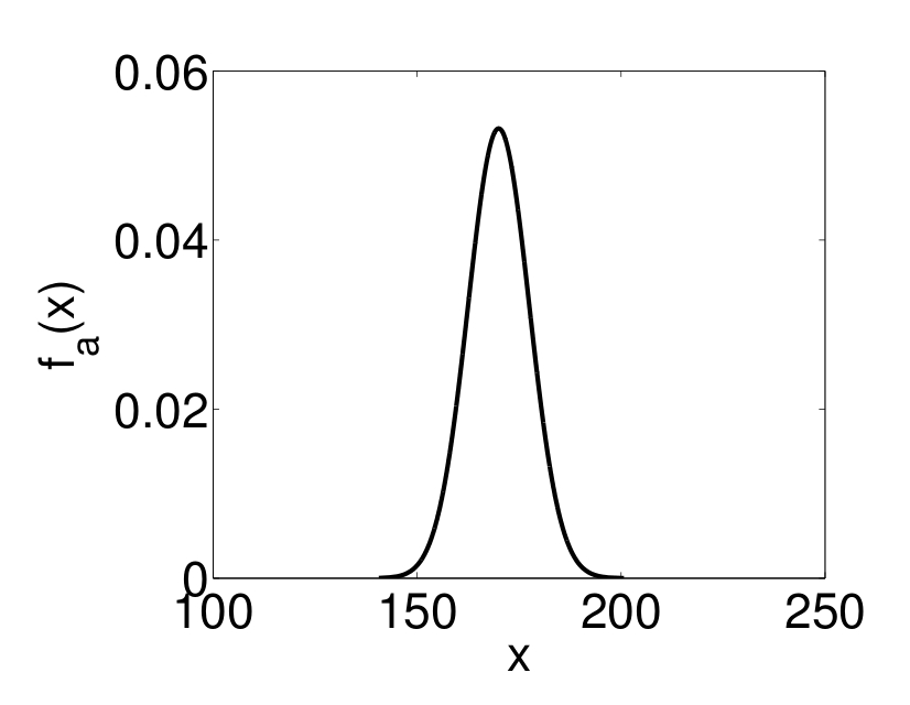
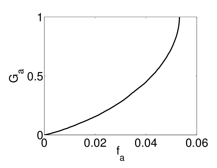
Assume that the height of the individuals of a population is normally distributed with mean $\mu=170cm$ and standard deviation $\sigma=7.5cm$. Then, let $a$ be the attribute representing the height, $X_{a}$ is a random variable following the same distribution of the domain and $f_{a}(x)$ is the associated pdf, reported in the first graph of fig. 1. The pdf $f_{a}(x)$ assumes value in the domain $[0,f_{a}(\mu)=0.0532]\subset\mathbb{R}$. Consider, now, the random variable $X^{f}_{a}$. The cdf $G_{a}(v)$ associated with $X^{f}_{a}$ denotes the probability for $f_{a}$ to assume value less than or equal to $v$. Then, $G_{a}(v)=0$ for each $v\leq 0$ and $G_{a}(v)=1$ for each $v\geq 0.0532$. To compute the value of $G_{a}(v)$ for a generic $v$, the integral reported in Equation (1) has to be evaluated. The resulting function is reported in the second graph of fig. 1.

Figure 1: Example of function $G_{a}(\cdot)$.

The outlierness ${\rm out}_{a}(o,{\it DB})$ (or, simply, ${\rm out}_{a}(o)$) of the attribute $a$ in $o$ w.r.t. ${\it DB}$ is defined as follows:

$${\rm out}_{a}(o)=\Omega\left(\int_{f_{a}(o[a])}^{+\infty}(1-G_{a}(f))~{}{\rm d}f-\int_{0}^{f_{a}(o[a])}G_{a}(f)~{}{\rm d}f\right),$$ (2)

where $\Omega$ denotes a suitable function mapping $\mathbb{R}$ to $[0,1]$ such that ($i$) $\Omega(x)=0$ for $x<0$, and ($ii$) $\Omega$ is monotone increasing for $x\geq 0$. In the following we employ the mapping

$$\Omega(x)=\frac{1-\exp(-x)}{1+\exp(-x)}.$$

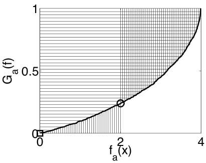
The first integral measures the area above the cdf $G_{a}(f)$ for $f>f_{a}(o[a])$, while the second integral measures the area below the cdf $G_{a}$ for $f\leq f_{a}(o[a])$. Intuitively, the larger the first term, the larger the degree of unbalanceness between the occurrence probability of $o[a]$ and that of the values that are more probable than $o[a]$. As for the second term, the smaller it is, the more likely the value $o[a]$ to be rare. Thus, the outlierness value ranges within $[0,1]$ and in particular it is close to zero for usual properties. By contrast, values closer to one denote exceptional properties.

Example 2

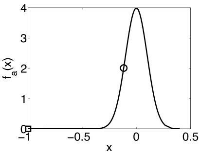
Consider fig. 2, reporting on the left a Gaussian distribution $f_{a}(x)$ (with mean $\mu=0$ and standard deviation $\sigma=0.1$). Consider the values $v_{1}=-1$ and $v_{2}=-0.12$, for which $f_{a}(v_{1})\approx 0$ and $f_{a}(v_{2})\approx 2$ hold. Assume that an outlier object $o$ exhibits value $v_{1}$ on $a$. The associated outlierness ${\rm out}_{a}(o)$ corresponds to the whole area (filled with horizontal lines) above the cdf curve, that is $\Omega(3.06)=0.91$. For an object $o^{\prime}$ exhibiting value $v_{2}$ on $a$, instead, the associated outlierness corresponds to the difference between two areas (filled with vertical lines) detected at frequency $2$, that is $\Omega(1.17-0.10)=0.49$.

Figure 2: Example of outlierness measure.

For the sake of clarity, in the above example we considered a pdf having a simple form. However, we wish to point out that our measure is able to correctly recognize exceptional properties irrespectively of the form of the underlying pdf, since it compares the occurrence probabilities of the domain values rather than directly comparing the original domain values.

Given an object $o$ and a dataset ${\it DB}$ on a set of attributes $\mathbf{A}$, an attribute $p\in\mathbf{A}$ showing a large (i.e. exceeding a given threshold) value ${\rm out}_{p}(o,{\it DB})$ of outlierness will be called a (outlying) property of $o$ in ${\it DB}$.

2.2 Explanations

Explanations are useful in our framework to provide a justification of the anomalous value characterizing an outlier. Intuitively, an attribute $a\in\mathbf{A}$ of $o$ that behaves normally with respect to the database as a whole, may be unexpected when the attention is restricted to a portion of the database. Relevant subsets of the database upon which to investigate outlierness can be hence obtained by selecting the database objects satisfying a condition, and such that a property is exceptional for $o$.

A condition $c$ (set of conditions $C$, resp.) is, intuitively, an explanation of the property $a$, if $o\in{\it DB}_{c}$ ($o\in{\it DB}_{C}$, resp.) and $a$ is an outlying property of $o$ in ${\it DB}_{c}$ (${\it DB}_{C}$, resp.). Finally, the outlierness of the attribute $a$ in $o$ w.r.t. $DB$ with explanation $C$ is defined as ${\rm out}_{a}^{C}(o,{\it DB})={\rm out}_{a}(o,{\it DB}_{C})$.

It is worth noticing that, according to the relative size of ${\it DB}_{C}$, not all the explanations should be considered equally relevant. In the following, we concentrate on $\sigma$-explanations, i.e., conditions $C$ such that $\frac{|{\it DB}_{C}|}{{\it DB}}\geq\sigma$, where $\sigma\in[0,1]$ is a user-defined parameter.

Thus, given an object $o$ of a database ${\it DB}$ on a set of attributes A, and parameters $\sigma_{\theta}\in[0,1]$ and $\Omega_{\theta}\in[0,1]$, the problem of interest here is: Find the pairs $(E,p)$, with $E\subseteq\mbox{\bf A}$ and $p\in\mbox{\bf A}\setminus E$, such that $E$ is a $\sigma_{\theta}$-explanation and ${\rm out}_{p}^{E}(o,{\it DB})\geq\Omega_{\theta}$.

The pair $(E,p)$ is also called an (outlier) explanation-property pair of $o$ in ${\it DB}$.

3 Detecting Outlying Properties

In order to detect outlying properties and their explanations, we need to solve two basic problems: (1) computing the outlierness of a certain multiset of values and (2) determining the conditions to be employed to form explanations. The strategies we have designed to solve these two problems exploit a common framework, which is based on Kernel Density Estimation (KDE). Specifically, given a numerical attribute $a$, in order to estimate the pdf $f_{a}$ we exploit generalized kernel density estimation [16], according to which the estimated density at point $x\in\mathbb{D}(a)$ is

$$\hat{f}_{{\bf m},{\bf w},{\bf b}}(x)=\left(\sum_{i=1}^{k}w_{i}\right)^{-1}\sum_{i=1}^{k}\frac{w_{i}}{b_{i}}K\left(\frac{x-m_{i}}{b_{i}}\right),$$ (3)

Here, $K$ is a kernel function, and ${\bf m}=(m_{1},\ldots,m_{k})$, ${\bf w}=(w_{1},\ldots,w_{k})$ and ${\bf b}=(b_{1},\ldots,b_{k})$ are $k$-dimensional vectors denoting the kernel location, weight, and bandwidth, respectively. The above mentioned strategies are detailed next, together with the method for mining outlying properties.

3.1 Outlierness computation

In order to compute the outlierness, we specialize formula in Equation (3) by setting ${\bf m}=(x_{1},\ldots,x_{n})$ and ${\bf w}={\bf 1}$, thus obtaining

$$\hat{f}_{a}(x)=\frac{1}{n}\sum_{i=1}^{n}\frac{1}{b_{i}}K\left(\frac{x-m_{i}}{b_{i}}\right),$$ (4)

where $x_{1},\ldots,x_{n}$ are the values in $\{y[a]:y\in{\it DB}\}$, each term $b_{i}$ is equal to $h\beta_{i}$, with $h$ a global bandwidth (as a rule of thumb, the global $h$ is set to $1.06\cdot{\rm std}({\bf x})\cdot n^{-1/5}$) and $\prod_{i=1}^{n}\beta_{i}=1$.

The rationale underlying this choice is that we want that each value at hand (${\bf m}={\bf x}$) contributes in equal manner (${\bf w}={\bf 1}$) to the estimation of the underlying pdf. Moreover, we employ the Parzen window kernel function, that is $K(x)=1$, for $|x|\leq 1/2$, and $K(x)=0$ otherwise, since this kernel represents a good trade off between simplicity of computation and accuracy. Indeed, the above density estimate can be computed in time $O(n\log n)$ by means of a sort of the attribute domain.

We also notice that, since the outlierness depends on the cdf of the pdf values, this greatly mitigates the impact of the non-smoothness of the estimate of the pdf through Parzen windows, other than making the measure robust w.r.t. deviations of the estimate from the real distribution.

3.2 Condition building

Proper conditions are the basic building blocks for the explanations. To single them out, our strategy consists in finding, for each attribute $a$, the “natural” interval $I_{a}$ including $o[a]$, namely, an interval of homogeneous values on $a$. Natural intervals, in our modeling, represent a partitioning of $\mathbb{D}(a)$ according to the density $f_{a}(x)$: intuitively, an interval is a high density area separated by another interval by a low-density area.

The search for feasible intervals still relies on adopting the kernel density family introduced so far, but according to a different interpretation. In practice, for each attribute $a$, we estimate $f_{a}$ by means of $\hat{f}_{\mathbf{m},\mathbf{w},\mathbf{b}}$. This latter function can be interpreted as a mixture density over the parameter sets $\mathbf{m},\mathbf{w},\mathbf{b}$. Hence the intervals can be obtained by estimating such parameters. To this purpose, we adopt the Gaussian kernel $K(x)=\phi(x)=(2\pi)^{-1/2}\exp(x^{2}/2)$ and devise the simplifying latent assumption that each data point is generated by a unique kernel location. This allows us to adopt an EM-based maximum likelihood approach, where the resulting iterative scheme draws from [16], and updates locations and bandwidths according to the following equations:

$$m_{j}=\frac{1}{\sum_{i}\gamma_{ij}}\sum_{i=1}^{n}x_{i}\gamma_{ij},\qquad\qquad\!\!b_{j}^{2}=\frac{1}{\sum_{i}\gamma_{ij}}\sum_{i=1}^{n}\gamma_{ij}(x_{i}-m_{j})^{2}$$ (5)

Here, $\gamma_{ij}$ represents the mixing probability that value $i$ is associated with the $j$-th kernel location and, in its turn, is computed at each iteration as:

$$\gamma_{ij}=\frac{w_{j}\phi_{b_{j}}(x_{i}-m_{j})}{\hat{f}_{\mathbf{m},\mathbf{w},\mathbf{b}}(x_{i})}$$ (6)

We also adapt the annihilation procedure proposed in [14], which allows for an automatic estimation of the optimal number $k^{\ast}$ of kernel locations, as well as to ignore the initialization issues. The estimation of the parameters is accomplished iteratively for each location$j$, where each weight is computed as

$$w_{j}=\frac{\max\{0,\sum_{i=1}^{n}\gamma_{ij}-\frac{n}{2}\}}{\sum_{j=1}^{k^{\ast}}\max\{0,\sum_{i=1}^{n}\gamma_{ij}-\frac{n}{2}\}}$$ (7)

Whenever a weight equals to $0$, the contribution of its component annihilates in the density estimation. As a consequence, the iterative procedure can start with a high initial value $k^{\ast}$, and the initialization of each mixing probability can be done randomly without compromising the final result. To summarize, the overall scheme can be described as follows:

1. Initialize $\gamma_{ij}$ randomly.

2. For each $j$ compute $w_{j}$; if $w_{j}\neq 0$ then update $m_{j}$ and $b_{j}$.

3. Recompute $\gamma_{ij}$ and return to step 2, until the improvement in likelihood is negligible.

The natural interval of $o$ in $a$ w.r.t. ${\it DB}$ can be obtained by exploiting the $\gamma_{ij}$ values. First of all, each $x_{i}$ can be assigned to a location $k_{i}=\arg\max_{j}\gamma_{ij}$. Then, let $\overline{k}$ be the location wich $o[a]$ is assigned to. The interval $I_{a}$ is then uniquely identified by $[l_{a},u_{a}]$, where $l_{a}=\min_{i}\left\{x_{i}\mid k_{i}=\overline{k}\right\}$ and $u_{a}=\max_{i}\left\{x_{i}\mid k_{i}=\overline{k}\right\}$.

Input: $o$ : an outlier object
${\it DB}$ : a dataset

Output: $\cal OP$ : the set of minimal explanation-property pairs of $o$ in ${\it DB}$

// First phase

1 foreach attribute $a_{i}\in\mbox{\bf A}$ do

2       Compute interval $I_{a_{i}}$;

3      

// Second phase

4 foreach attribute $p\in\mbox{\bf A}$ do

5       set $L_{1}$ to $\{c_{i}\equiv a_{i}\in I_{a_{i}}\mbox{ s.t. }|{\it DB}_{c_{i}}|/|{\it DB}|\geq\sigma_{\theta}\}$;

6       set $j$ to $2$;

7       while $j\leq k_{\theta}$ and $L_{j-1}\neq\emptyset$ do

8             set $E_{j}$ to $\{C\cup\{c\}\mbox{ s.t. }C\in L_{j-1}\mbox{ and }c\in\bigcup L_{j-1}\mbox{ and }c\not\in C\}$;

9             foreach $C\in E_{j}$ do

10                   if $|{\it DB}_{C}|/|DB|\geq\sigma_{\theta}$ then

11                         if ${\rm out}_{p}^{C}(o,{\it DB})\geq\Omega_{\theta}$ then

12                               set $\cal OP$ to ${\cal OP}\cup\{(C,p)\}$;

13                              

14                        else

15                               set $L_{j}$ to $L_{j}\cup\{C\}$;

16                              

17                        

18                  

19            set $j$ to $j+1$;

20            

21      

return $\cal OP$

Algorithm 1 Outlying Property Detector($o,a,{\it DB}$)

3.3 The mining method

Given a dataset ${\it DB}$ on the set of attributes $\mbox{\bf A}=\{a_{1},\ldots,a_{m}\}$, an outlier object $o$, parameters $\sigma_{\theta}\in[0,1]$, $\Omega_{\theta}\in[0,1]$, and positive integer $k_{\theta}\leq m$ (representing an upper bound to the size of an acceptable explanation), the algorithm Outlying-Property Detector computes all the pairs $(E,p)$, with $|E|\leq k_{\theta}$ and $p\in\mbox{\bf A}\setminus E$, such that:

1. $E$ is a $\sigma_{\theta}$-explanation, and

2. the outlierness ${\rm out}_{p}^{E}(o,{\it DB})$ is not smaller than $\Omega_{\theta}$, and

3. $(E,p)$ is minimal, that is there is not a pair $(E^{\prime},p)$ with $E^{\prime}\subset E$ for which both points 1 and 2 hold.

The algorithm consists of two main phases. During the first phase, for each attribute $a_{i}\in\mbox{\bf A}$, the interval $I_{a_{i}}$ and, hence, the associated condition $a_{i}\in I_{a_{i}}$, is determined by means of the procedure described in Section 3.2. Given the set of conditions $S=\{a_{1}\in I_{a_{1}},\ldots,a_{m}\in I_{a_{m}}\}$ on the $m$ attributes in A, the second phase exploits an apriori-like strategy [2] in order to search for the pairs $(E,p)$ with $E\subseteq S$ meeting the above mentioned conditions. The computed pairs are accumulated in the set ${\cal OP}$, which represents the output of the algorithm.

The parameter $k_{\theta}$ here is introduced in order to bind the size of an acceptable explanation. As a matter of fact, greater values of $k_{\theta}$ trigger larger explanations which are likely to lower the support to unacceptable values. Also, large explanations result difficult to interpret. Notice that by setting $k_{\theta}$ to the value $m$ all the pairs can be mined. In the experimental section we study the effects of the $k_{\theta}$ parameter on the performances.

As for the cost of the above procedure, the first step is basically depends on the rate of convergence of the EM algorithm. By assuming that the number $k$ of kernel locations is initially set to $\sqrt{n}$, the basic iteration is $O(n^{3/2})$. Notice, however, that interval components annihilate early in the first iterations, so practically we can assume that the number of intervals $k^{\ast}$ is bounded to a constant value. Thus, the overall complexity of the first step is linear in the size of the data and the number of iterations. Clearly, the rate of convergence of the algorithm is also of practical interest, and it is usually slower than the quadratic convergence typically available with Newton-type methods. [13] shows that the rate of convergence of the EM algorithm is linear and the it depends on the proportion of information in the observed data.

As far as the second step is concerned, computing the outlierness costs $O(n\log n)$. Since these two sub-steps are executed at most $O(m^{k_{\theta}})$ times, the overall cost of step 2 is $O(m^{k_{\theta}}n\log n)$. However, notice that the apriori-like strategy greatly reduces the size of portion of the search space to be explored, so that the total number of conditions explored in practice is much smaller.

4 Experimental results

We evaluate the technique on both real-life and synthesized datasets, with the aim of showing the effectiveness of the proposed approach. The ground truth in such datasets is represented by outlier tuples, detected by resorting to the feature bagging algorithm described in [19]. Briefly, the technique detects outliers by iteratively running a base outlier detection algorithm on a subset of the available attributes. Outlier detected in the various runs are then scored by adopting a combine function which assigns a score to each outlier.

The bagging technique was instantiated by exploting the base OD method described in [4], where the parameters are set to produce just a single outlier. Further, the combine technique adopted simply scores outliers on the basis of the positive responses they get within the iterations: if a tuple is detected as an outlier in a given iteration, it gets a positive score. Scores are then summarized in the combine function, and tuples are sorted according to the scores.

The feature bagging technique boosts the robustness of base outlier detection techniques. By contrast, it is difficult to manually infer (e.g., by means of visualization techniques) justification for outlierness: A tuple can be reputed an outlier for a combination of factors which in turn depend on different subsets of the attributes. As a consequence, the analysis of the outliers produced with such a technique provides a significant benchmark on the effectiveness of the outlier explanation technique.

We employ three real datasets from the UCI Machine Learning repository [15]. The first two datasets, namely Ecoli (with $336$ instances and $7$ attributes) and Yeast (with $1,\!484$ instances and $8$ attributes), contain information about protein localization sites. The third database, called Cloud, contains information about cloud cover and includes $1,\!024$ instances with $10$ attributes.

The support threshold $\sigma_{\theta}$ has been set to $0.2$ and the maximum number $k_{\theta}$ of conditions in the explanation to $3$. The following table reports the explanation-property pairs scoring the maximum value of outlierness.

$\bf DB$	$\bf o$	$\bf{out}_{p}^{E}(o)$	$\bf p$	$\bf E$
Ecoli	223	1.000	$a_{4}$	$\emptyset$
Yeast	990	0.997	$a_{3}$	$\{~{}a_{2}\in[0.13,0.38]~{}\}$
Cloud	354	1.000	$a_{6}$	$\begin{array}[]{ll}\{&a_{1}\in[1.0,6.7],\\ &a_{2}\in[134.9,255.0],\\ &a_{5}\in[2,\!450.5,3,\!211.5]~{}\}\end{array}$

In the third column, we report the outlierness value, in the fourth column the attribute associated with the property, and in the fifth column the explanation. Figure 3 reports the functions $G_{a}(f)$ associated with the objects considered in the experiments.

Figure 3: Experimental results on the Ecoli, Yeast, and Cloud datasets.

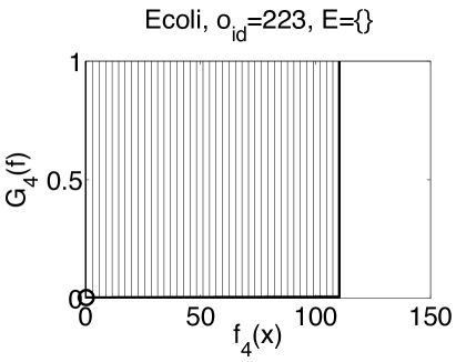
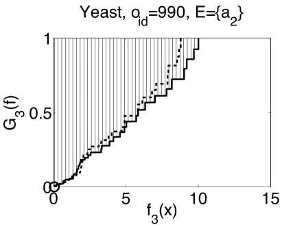
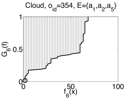
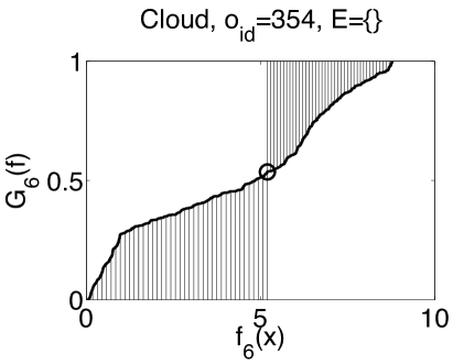
Figure 3 at the top left reports the area associated with the property $a_{4}$ and empty explanation for the object $223$ in the Ecoli database. The property $a_{4}$ is the attribute Presence of charge on N-terminus of predicted lipoproteins. The object $223$ is the only object assuming value $0.5$ on this attribute, while all the other objects assume value $1.0$. As a consequence, this attribute is a clear outlying property with respect to the whole database and, in fact, the associated explanation is empty.

Figure 3 at the top right reports the area associated with the property $a_{3}$ for the object $990$ in the $Yeast$ database. The attribute $a_{3}$ is Score of the ALOM membrane spanning region prediction program. The solid line represents the curve $G_{a_{3}}(f)$ obtained when the explanation relative to attribute $\{a_{2}\}$ is taken into account, while the dashed line represents the curve $G_{a_{3}}(f)$ obtained for the empty explanation. There is a limited improvement in the significance of the outlierness degree when the explanation is taken into account, as shown by the distance in the two lines.

Things are substantially different with object $354$ in the Cloud database. Figure 3 at the bottom left reports the area associated with the property $a_{6}$ and the explanation $\{a_{1},a_{2},a_{5}\}$. The attribute $a_{6}$ is the Visible entropy, while the explanation attributes are Visible mean, Visible max and Contrast. Figure 3 on the bottom right reports the area associated with the same property, but for an empty explanation. Clearly, property $a_{6}$ is not exceptional with respect to the whole dataset, but it becomes very exceptional with respect to the subpopulation selected by the explanation.

The following table reports the execution times associated with the experiments.

DB	Condition	Outlier
	Building	Computation
Ecoli	6.39 sec	16.76 sec
Yeast	54.38 sec	138.51 sec
Cloud	702.67 sec	91.08 sec

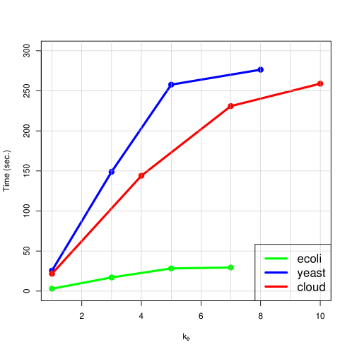
It can be noticed that the time is split into the two main operations, namely the identification of intervals, and the computation of the outlierness degree. The two routines tend to balance the cost of the overall computation. However, since the parameter $k_{\theta}$ is likely to affect the performance of the outlier computation, we study the latter on increasing value of the parameter. As a matter of fact, greater values of $k_{\theta}$ trigger larger explanations which are likely to lower the support to unacceptable values. Figure 4 plots the Total Outlier Computation Time for increasing values of $k_{\theta}$. The curves tend to flatten for increasing values, on all datasets, as an affect of the shrinking of $\mathit{DB}_{C}$ when $C$ tends to become large.

Figure 4: Total Outlier Computation Time for Ecoli, Yeast, and Cloud datasets.

It is natural to ask whether the computation of the outlierness degree based on kernel density estimation provides a true advantage over the alternative approach of first discretizing the attributes, and then applying the originary method described in [5]. To this aim, we perform further tests on synthesized data. In particular, we generate a dataset (named Unif2 in the following), consisting of $20,\!000$ objects. This dataset contains an outlier $o$ which is distinguished from the rest of the population from the value it assumes on a particular attribute $A$. Specifically, almost all values of this attribute belong to two equally-sized uniformly distributed clusters, the first one in the range $[-1.1,-0.1]$ and the second one in the range $[0.1,1.1]$. The only exception is represented by the object $o$, for which $o[A]=0$ holds. In the following, we concentrate the comparison on the analysis of the behavior of the two methods on the attribute $A$, in order to demonstrate that while $A$ is naturally perceived as an outlying property by the technique hereby introduced, it is very unlikely to obtain the same goal when the technique in [5] is employed.

Figure 5: Unif2 dataset: outlierness of $A$ in $o$ computed using the method in [5] (on the left), and density estimate of the same attribute carried out by our method (on the right).

Figure 6: Different equi-width histograms associated with the attribute $A_{U2}$ of the Unif2 data set.

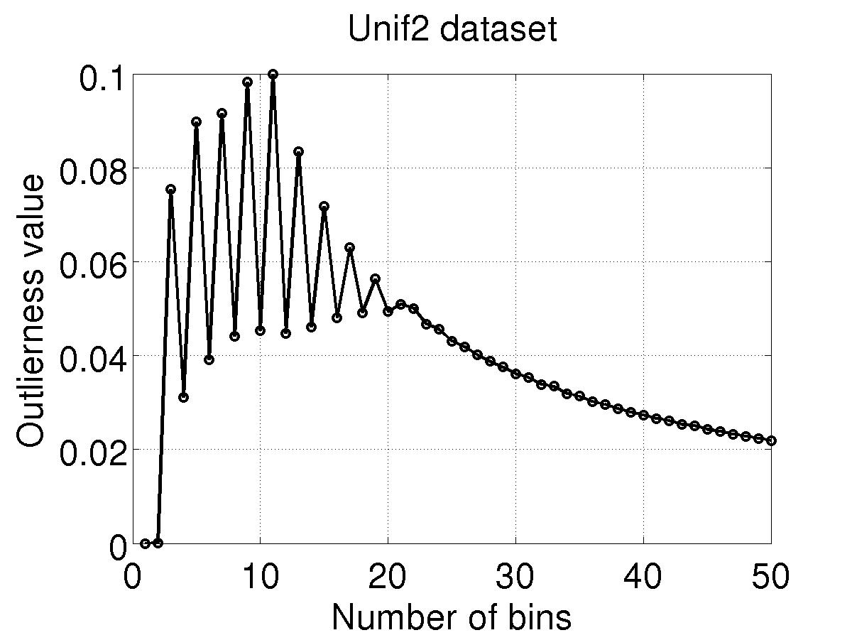
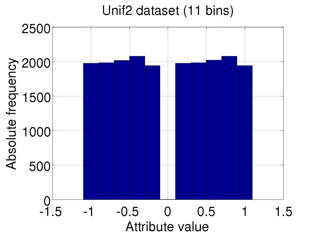
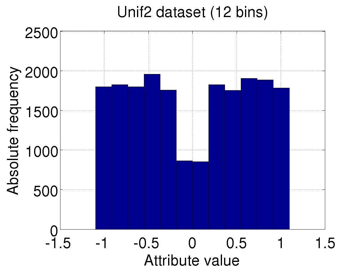
In order to apply the latter method to the Unif2 dataset, we discretize the attributes by grouping attribute values in equi-width bins. Figure 5 reports on the left the value of the outlierness (as defined in [5]) on the value $o[A]$ according to different bins sizes employed in discretizing the data. Specifically, the number of bins has been varied from $2$ to $50$. The experiment highlights that when the method in [5] is applied, the outcome of the analysis strongly depends on the discretization adopted. In particular when the number of bins is in the range $[4,20]$ the outlierness measure fluctuates between 0.3 and 1. This means that even small changes in the number of bins produce results which can dramatically change. This is a very undesirable property, since determining the right number of bins for the analysis at hand is a very challenging task.

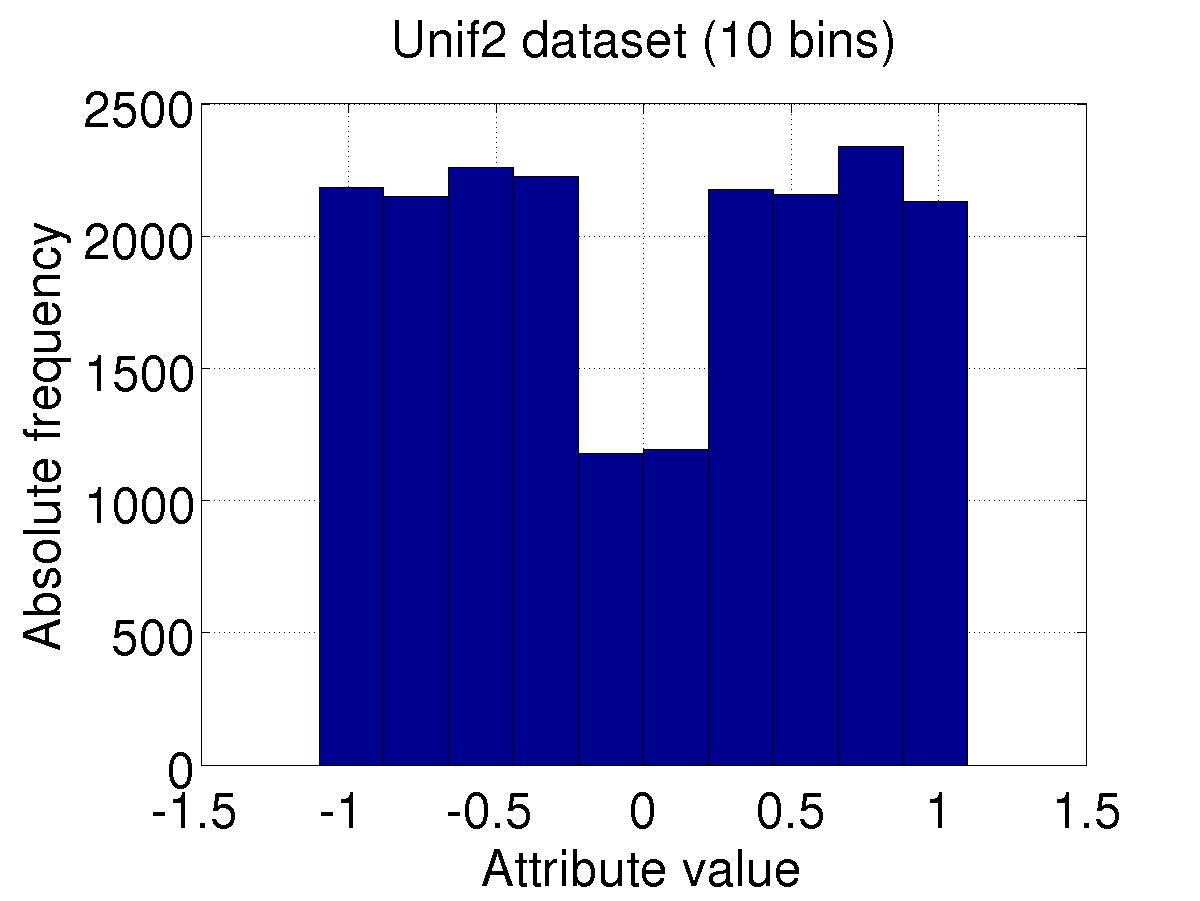
Figure 6, showing different frequency histograms associated with the attribute $A$, should further clarify things. The histogram associated with the best outlierness value, namely outlierness $0.1$, is the one using $11$ bins (at the center of the figure). In this case, the central bin (centered in zero) scores a low value of absolute frequency. Differently, for both $10$ bins (reported on the left in the same figure) or $12$ bins (reported on the right), the fact that the outlierness of $A$ in $o$ is sensibly smaller can be explained by looking at the displayed histograms. In both cases, the value of $o$ is grouped with some more frequent values and, hence, the corresponding outlierness value gets sensibly smaller.

Providing a larger number of bins does not solve the problem: as already pointed out, the scoring functions assigns a score close to $1$ to very unbalanced distributions, while its value rapidly decreases when frequencies spread. And, indeed, with a large bin size the number of different categorical values (each associated with a different bin) becomes large, and these values score about the same absolute frequency. The consequence is that the outlierness values get small as well.

We can conclude that in order to enable the method [5] to discover meaningful knowledge, the bins that maximize the score should be detected in the first place. However, the interaction with explanations (which select subsets of the overall population) makes it difficult to provide optimal a-priori intervals, since the distribution of the property attribute are likely to change when switching from one explanation to another.

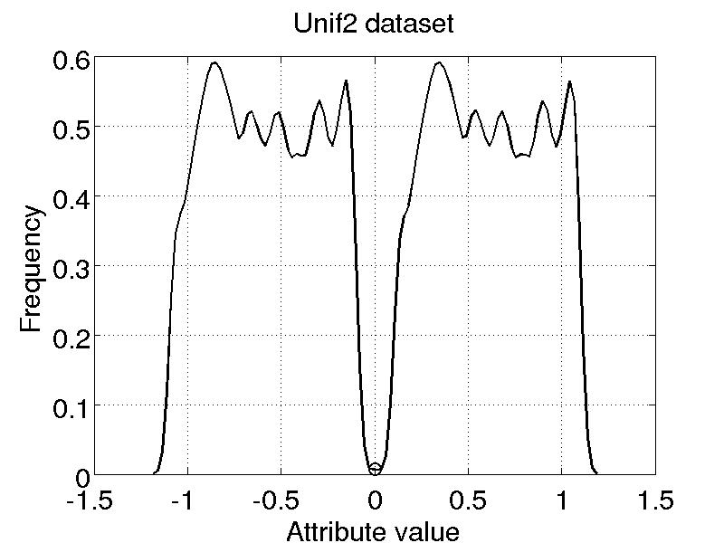
This is clearly not the case with the technique proposed in this paper. Since the outlierness measure defined here directly exploits the density estimate of the object value, it is completely adaptive to numerical data and does not suffer of the aforementioned drawbacks. The outlierness computed by our method is $0.775$. Figure 6 on the right shows the density estimate of attribute $A$, together with the value associated to $o$ (notice the circle on the curve), which is exploited in order to compute the outlierness associated with $o$.

5 Conclusions and Future Work

The purpose of this paper has been that of devising techniques by which the outlying properties detection problem can be solved in the presence of both categorical and numerical attributes, which represents a step forward with respect to available literature. The core of our approach has been the definition of a sensible outlierness measure, representing a refined generalization of that proposed in [5], which is able to quantify the exceptionality of a given property featured by the given input anomalous object with respect to a reference data population. Also, we have developed algorithms to detect properties characterizing the anomalous object provided in input. The experimental results we have obtained confirm that the presented approach is more than promising.

As a matter of fact, there are several application scenarios where the proposed technique can be profitably applied. Further scenarios include rank learning problems like in [12]: there, the problem of detecting rules for characterizing individuals who are scored as exceptional according to a specific scoring function (like, e.g., the amount of fraud they commit in a fraud detection scenario) is investigated. It is clear that if exceptional objects are reputed as outliers, then the outlier explanation technique described in this paper could be exploited as a basic building block for rule learning in that domain.

As future work, we are interested in exploring other strategies for generating proper conditions and in exnteding the experimental campaign.

References

- [1] C. C. Aggarwal and P.S. Yu. Outlier detection for high dimensional data. In Proc. of the International Conference on Managment of Data (SIGMOD), pages 37–46, 2001.
- [2] Rakesh Agrawal and Ramakrishnan Srikant. Fast algorithms for mining association rules in large databases. In VLDB, pages 487–499, 1994.
- [3] F. Angiulli, S. Basta, and C. Pizzuti. Distance-based detection and prediction of outliers. IEEE Transaction on Knowledge and Data Engineering, 2(18):145–160, February 2006.
- [4] F. Angiulli and F. Fassetti. Dolphin: an efficient algorithm for mining distance-based outliers in very large datasets. ACM Transactions on Knowledge Discovery from Data, 3(1):Article 4, 2009.
- [5] F. Angiulli, F. Fassetti, and L. Palopoli. Detecting outlying properties of exceptional objects. ACM Transactions on Database Systems, 34(1):Article 7, 2009.
- [6] F. Angiulli, F. Fassetti, and L. Palopoli. Discoverying characterizations of the behavior of outlier sub-populations. IEEE Transactions on Knowledge and Data Engineering, doi:10.1109/TKDE.2012.58, published online, March 19, 2012.
- [7] F. Angiulli and C. Pizzuti. Outlier mining in large high-dimensional data sets. IEEE Trans. Knowl. Data Eng., 2(17):203–215, February 2005.
- [8] V. Barnett and T. Lewis. Outliers in Statistical Data. John Wiley & Sons, 1994.
- [9] M. M. Breunig, H. Kriegel, R.T. Ng, and J. Sander. Lof: Identifying density-based local outliers. In Proc. International Conference on Managment of Data (SIGMOD), pages 93–104, Dallas, TX, USA, 2000.
- [10] V. Chandola, A. Banerjee, and V. Kumar. Anomaly detection: A survey. ACM Computing Surveys, 41(3), 2009.
- [11] N. V. Chawla, N. Japkowicz, and A. Kotcz. Editorial: special issue on learning from imbalanced data sets. SIGKDD Explorations, 6(1):1–6, 2004.
- [12] Gianni Costa, Fabio Fassetti, Massimo Guarascio, Giuseppe Manco, and Riccardo Ortale. Mining models of exceptional objects through rule learning. In SAC, pages 1078–1082, 2010.
- [13] A. P. Dempster, N. M. Laird, and D. B. Rubin. Maximum likelihood from incomplete data via the EM algorithm. Journal of the Royal Statistical Society, B, 39, 1977.
- [14] M. A. T. Figueiredo and A. K. Jain. Unsupervised learning of finite mixture models. IEEE Transactions on Pattern Analysis and Machine Intelligence, 24:381–396, 2002.
- [15] A. Frank and A. Asuncion. Uci machine learning repository [archive.ics.uci.edu/ml], 2010.
- [16] M. C. Jones and D. A. Henderson. Maximum likelihood kernel density estimation: On the potential of convolution sieves. Computational Statistics & Data Analysis, 53:3726–3733, 2009.
- [17] E. Knorr and R. Ng. Algorithms for mining distance-based outliers in large datasets. In Proc. of the International Conference on Very Large Databases (VLDB), pages 392–403, New York, NY, USA, 1998.
- [18] E. Knorr and R. Ng. Finding intensional knowledge of distance-based outliers. In Proc. Int. Conf. on Very Large Databases (VLDB99), pages 211–222, 1999.
- [19] Aleksandar Lazarevic and Vipin Kumar. Feature bagging for outlier detection. In Proc. of ACM SIGKDD Conf (KDD’05), pages 157–166, 2005.
- [20] F.T. Liu, K.M. Ting, and Z.-H. Zhou. Isolation forest. In Proc. of the IEEE International Conference on Data Mining (ICDM), pages 413–422, Pisa, Italy, 2008.
- [21] S. Papadimitriou, H. Kitagawa, P.B. Gibbons, and C. Faloutsos. Loci: Fast outlier detection using the local correlation integral. In Proc. of the International Conference on Data Enginnering (ICDE), pages 315–326, Bangalore, India, 2003.
- [22] B. Schölkopf, C. Burges, and V. Vapnik. Extracting support data for a given task. In Proc. of the ACM SIGKDD International Conference on Knowledge Discovery and Data Mining (KDD), pages 252–257, Montreal, Canada, 1995.