A Continuum Generalization of the Ising Model

Abstract

The Lenz-Ising model has served for almost a century as a basis for understanding ferromagnetism, and has become a paradigmatic model for phase transitions in statistical mechanics. While retaining the Ising energy arguments, we use techniques previously applied to sociophysics to propose a continuum model. Our formulation results in an integro-differential equation that has several advantages over the traditional version: it allows for asymptotic analysis of phase transitions, material properties, and the dynamics of the formation of magnetic domains.

Introduction—The Ising Model is a widely-studied model for magnetic phenomena Domb (1976); de Jongh and Miedema (1974) which posits that each particle in a material has associated with it a binary magnetic polarity, or “spin,” that may flip to reduce the energy of the system. Derived as an equilibrium model in statistical mechanics, results for one-dimensional nearest-neighbor coupling were presented by Ising in his 1924 doctoral thesis Ising (1925). An exact solution for two-dimensional nearest-neighbor coupling was found in 1944 by Onsager Onsager (1944), spurring a flurry of research in the mid-twentieth century. Since then the Ising model has motivated thousands of peer-reviewed publications and become fundamental to understanding phase transitions Stanley (1999).

While research on the Ising model has helped to provide insight into ferromagnetism and more general phase transitions, the statistical-mechanical approach has several disadvantages: traditional solutions to the Ising model cannot give information about the dynamics of phase transitions and approach to equilibrium; most results other than mean-field require laborious series expansions; no closed-form solution has been found in three dimensions, and such solutions are unlikely to be possible for irregular lattices.

Some of these drawbacks are remedied by simulating the Ising model numerically, following Monte-Carlo algorithms Metropolis et al. (1953); Binder (1976). However, numerical approaches do not provide much insight into dynamics, and the time required for simulation can be extremely long for large systems near critical points.

In this paper, we construct a continuous, deterministic model for ferromagnetism based on the energy arguments of the Ising model. This allows us to employ the tools of dynamical systems and perturbation theory to investigate time-dependence and asymptotic behavior for magnetization phenomena, as well as to recover mean-field results using new methods.

Our Model—In the statistical mechanics formulation of the Ising model, the system energy is given by

$$E=-\frac{1}{2}\sum_{i}\sum_{j}J_{ij}s_{i}s_{j}-\mu H\sum_{i}s_{i}~{},$$ (1)

where $J_{ij}$ defines the magnitude of coupling between spins $i$ and $j$ (their interaction energy), $H$ is the external magnetic field, and $\mu$ is the magnetic moment, which we set to 1 for convenience. We will take two continuum limits of Eq. (1).

Figure 1: Limit from discrete spin system to continuous system.

First, we introduce a spatial dimension along which magnetization may vary and take the coordinate $\xi\in[-1,1]$. A coupling kernel $G(\xi,\xi^{\prime})$ determines the interaction between spatial coordinates $\xi$ and $\xi^{\prime}$ (assumed to be periodic), and we retain $J$ as a constant coefficient, representing mean interaction energy for normalized $G(\xi,\xi^{\prime})$. Next, we further generalize the traditional binary spins $s=\pm 1$ to allow continuous $s\in[-1,1]$. We then write

$$E=-\frac{1}{2}J\int_{-1}^{1}\int_{-1}^{1}\!\!G(\xi,\xi^{\prime})s(\xi)s(\xi^{\prime})\,d\xi\,d\xi^{\prime}-H\int_{-1}^{1}\!\!s(\xi^{\prime})\,d\xi^{\prime}.$$

Computing the response to a differential change in $s$ at a single point in space, we find

$$\frac{\partial E}{\partial s}=-J\int_{-1}^{1}G(\xi,\xi^{\prime})s(\xi^{\prime})\,d\xi^{\prime}-H$$ (2)

(see Supplemental Material Section S1 for details on this derivation).

To describe the magnetization of the system, we use a “mass action” rate equation previously applied to sociophysics Abrams et al. (2011):

$$\frac{\partial x}{\partial t}=(1-x)P(x;u_{x})-xP(1-x;1-u_{x})~{}.$$

Here $x$ is the fraction belonging to one of two groups that partition the population and $u_{x}$ represents a relative bias towards this group. The function $P(x;u_{x})$ gives the probability per unit time that an individual will switch into this group. We adapt this equation to ferromagnetism first by making the change of variable $x=(s+1)/2$ so that the magnetization $s\in[-1,1]$. We reinterpret the function $P$ to now represent the probability per unit time that a particle in the magnetic material will switch polarity, now depending on an applied magnetic field $H$ instead of the social bias $u_{x}$.

In the discrete system, the probability that a particle will switch polarity is given by Glauber Glauber (1963) as inversely proportional to $1+\exp\left(\frac{\Delta E}{kT}\right)$, where $\Delta E$ is the incremental change in energy caused by the spin flip, $k$ is Boltzmann’s constant, and $T$ is temperature. Using the relationship $\Delta E\sim 2\frac{\partial E}{\partial s}$ (each discrete spin flip $\Delta s$ has magnitude 2), we modify the Glauber rate to depend on differential changes in spin:

$$P_{G}(s;H)\propto\left[1+\exp\left(\frac{2}{kT}\frac{\partial E}{\partial s}\right)\right]^{-1}~{}.$$ (3)

Using this expression for spin flip probability, our equation becomes

$$\frac{\partial s}{\partial t}=(1-s)P_{G}(s;H)-(1+s)P_{G}(-s;-H)~{}.$$ (4)

Note that time can be arbitrarily rescaled—a prefactor with units of inverse time has been set to one for convenience.

We may now write our full ODE system, combining the results of Eq. (2), (3), and (4). After some simplification, we find the integrodifferential equation describing system magnetization $s(\xi,t)$ for a general coupling kernel:

$$\frac{\partial s}{\partial t}=\tanh\!\left(\frac{J}{kT}\!\int_{-1}^{1}\!G(\xi,\xi^{\prime})s(\xi^{\prime},t)\,d\xi^{\prime}+\frac{H}{kT}\right)-s~{}.$$ (5)

Homogeneous System—In the case of spatially homogeneous magnetization, where $s(\xi,t)=m(t)$, Eq. (5) reduces to

$$\dot{m}=\tanh\left[\frac{1}{kT}\left(Jm+H\right)\right]-m~{}.$$ (6)

The fixed points of this equation are equivalent to solutions of the mean-field Ising model Domb (1976), but Eq. (6) also allows for prediction of dynamics. These dynamics are equivalent to the expected mean-field dynamics derived in Suzuki and Kubo (1968) using a master equation approach.

Analysis of Eq. (6) reveals a supercritical pitchfork bifurcation, as is expected (see Fig. 2). For zero temperature, the system must approach one of two stable fixed points $m^{*}=\pm 1$, while for temperatures above the bifurcation point $T_{c}=J/k$ (the Curie temperature), the sole fixed point is an unmagnetized (or “thermalized”) state, $m^{*}=0$. This solution also exists for $T<T_{c}$, but is unstable. Including a nonzero external field gives an imperfect pitchfork bifurcation, where $m=0$ is no longer a solution for finite nonzero temperatures. These fixed points are given implicitly by solutions to $T=(Jm^{*}+H)/(k\operatorname{arctanh}m^{*})$.

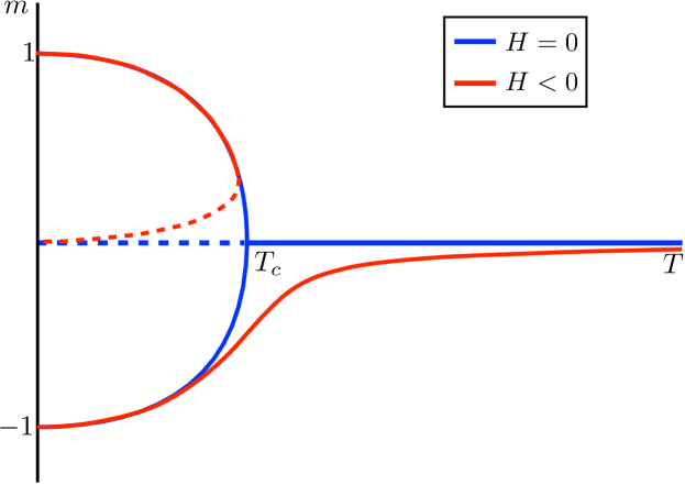
Figure 2: Steady-state magnetization versus temperature for homogeneous system, Eq. (6). For $H=0$ there is a supercritical pitchfork bifurcation, while for $H\neq 0$, the bifurcation becomes imperfect. Solid lines indicate stable solution branches, dashed unstable.

Piecewise-Constant System—The advantage of our formulation becomes clear when we relax the assumption of spatial homogeneity. As an illustrative example, we consider a perturbation off all-to-all coupling towards local coupling, assuming piecewise-constant spins. One possible application of such a system is in modeling regions of a ferromagnet separated by grain boundaries—perhaps of relevance for magnetic memory applications.

We let $s(\xi,t)$ be piecewise constant and assume that intra-grain coupling is stronger than inter-grain coupling:

$$s(\xi,t) =\begin{cases}m_{1}(t)&\text{if }\xi<0\\ m_{2}(t)&\text{if }\xi>0\end{cases}$$ (7)

$$G(\xi,\xi^{\prime}) =\frac{1}{2}(1+\delta\,\text{sgn}\,\xi\,\text{sgn}\,\xi^{\prime})~{}.$$ (8)

Then Eq. (5) becomes

$$\dot{m}_{1} =\tanh\left\{\frac{J}{2kT}\big{[}m_{1}(1+\delta)+m_{2}(1-\delta)\big{]}+\frac{H}{kT}\right\}-m_{1}$$

$$\dot{m}_{2} =\tanh\left\{\frac{J}{2kT}\big{[}m_{2}(1+\delta)+m_{1}(1-\delta)\big{]}+\frac{H}{kT}\right\}-m_{2}.$$

The coupling strength $\delta$ acts as a perturbation parameter, where $\delta=0$ recovers Eq. (6) for $\overline{m}=(m_{1}+m_{2})/2$ and $\delta=1$ separates the system into independent halves that each evolve separately according to Eq. (6). Thus, intermediate values $\delta\in(0,1)$ are of interest.

Fixed Points for Piecewise System—For all temperatures and all $\delta$, fixed points exist on the invariant manifold $m_{1}=m_{2}$, where the two halves of the system are aligned and evolve according to Eq. (6). Nontrivial fixed points may also be found on the invariant manifold $m_{1}=-m_{2}$: for $T<\delta$, besides $m_{1}^{*}=-m_{2}^{*}=0$, fixed points are also located at positions defined implicitly by $T=(J\delta m_{1}^{*}+H)/(k\operatorname{arctanh}m_{1}^{*})$. Those points are stable for $\delta>\frac{kT}{J}(1-\frac{kT}{J})^{-\frac{1}{2}}\operatorname{arctanh}(1-\frac{kT}{J})^{\frac{1}{2}}$, otherwise they become saddle points that merge at $m_{1}=-m_{2}=0$ as $T\to\delta$. See Figure 3 for a visualization of how fixed point stability changes with $T$ and $\delta$.

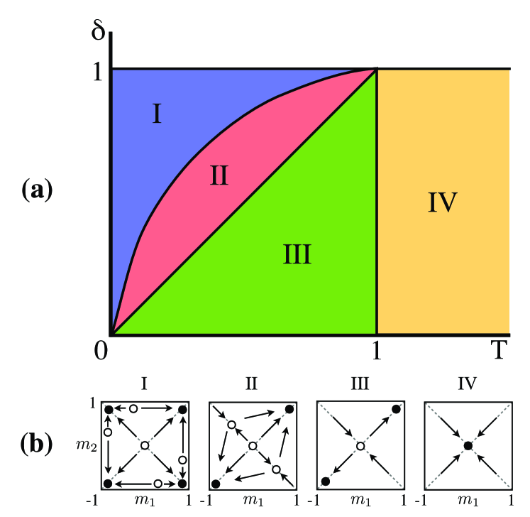
Figure 3: Fixed point locations and stability for piecewise-constant system. Shown in (a) are the regions of parameter space exhibiting qualitatively different behavior; the boundary between regions I and II is given approximately by $\delta=\frac{kT}{J}(1-\frac{kT}{J})^{-\frac{1}{2}}\operatorname{arctanh}(1-\frac{kT}{J})^{\frac{1}{2}}$. In (b), fixed point locations and stability are shown in phase space for each region; filled circles indicate stability, open circles instability. Arrows indicate direction of flow.

The existence of stable fixed points on the $m_{1}=-m_{2}$ manifold is difficult to predict with the traditional approach to the Ising model, but has important implications: it indicates that a critical temperature exists below which two ferromagnetic grains will not equilibrate.

Dynamics for Piecewise System—One benefit of modeling this system using a differential equation is that time-dependence is built in; we can evaluate the time scale of the approach to equilibrium by examining the system’s eigenvalues, which are especially straightforward to calculate in the piecewise constant system. For the fixed point at $m_{1}^{*}=m_{2}^{*}=0$ we find

$$\lambda_{1} =-1+\frac{J\delta}{kT},\quad\mathbf{v}_{1}=(-1,1)$$

$$\lambda_{2} =-1+\frac{J}{kT},\quad\mathbf{v}_{2}=(1,1)~{}.$$

Thus, along the antisymmetric manifold, the local time scale is $\tau_{1}\propto T/(T-\delta T_{c})$, and along the symmetric manifold, the local time scale is $\tau_{2}\propto T/(T-T_{c})$. These are relative thermalization times starting from either anti-aligned ($\tau_{1}$) or aligned ($\tau_{2}$) initial conditions.

Also of interest is the time it would take an unpolarized material to reach an equilibrium magnetization. In this case, it is straightforward to find the eigenvalues in terms of a general fixed point, either, $(m_{1}^{*},m_{2}^{*})=(m^{*},m^{*})$ or $(m_{1}^{*},m_{2}^{*})=(m^{*},-m^{*})$ . We then find time scales $\tau\propto(1-c\frac{1-m^{*2}}{m^{*}}\text{arctanh}\,m^{*})^{-1}$, where $c=1$ for flow perpendicular to the invariant manifolds, $c=\delta$ for flow along the aligned manifold (meaning $\tau$ increases with $\delta$), and $c=1/\delta$ for flow along the anti-aligned manifold (meaning $\tau$ decreases with $\delta$). In each case, the flow towards equilibrium is slower when $m^{*}$ is closer to zero.

Note that this analysis gives us insight into the different dynamics observed in regions II and III of Figure 3. Despite sharing similar stable equilibria, the structural change in unstable fixed points affects the time scale for equilibration. Observation of new time scales in numerical simulation would be difficult to account for without a theory that includes dynamics.

Von Mises Coupling—Although the simplicity of the piecewise constant system is appealing, it does not allow for smooth tuning between global (i.e. mean-field) and localized coupling. One coupling kernel that does allow such a continuous transition is the von Mises distribution

$$G(\xi,\xi^{\prime})=ce^{\kappa\cos\left[\pi(\xi-\xi^{\prime})\right]}~{},$$ (9)

with normalization constant $c=1/[2\,I_{0}(\kappa)]$. This distribution is similar to a Gaussian, but periodic. When the parameter $\kappa$ is large, the coupling is local, while $\kappa=0$ recovers global coupling.

We examined the equilibration time scale for this system, and found that the delay versus $\kappa$ curve is sigmoidal, behaving qualitatively like the piecewise constant system for $\kappa$ small. These results are shown in Figure 4. Intriguingly, for both the piecewise constant and von Mises coupling kernels, the locality can be tuned to produce the same equilibration delay as that observed on a nearest-neighbor lattice of arbitrary dimension.

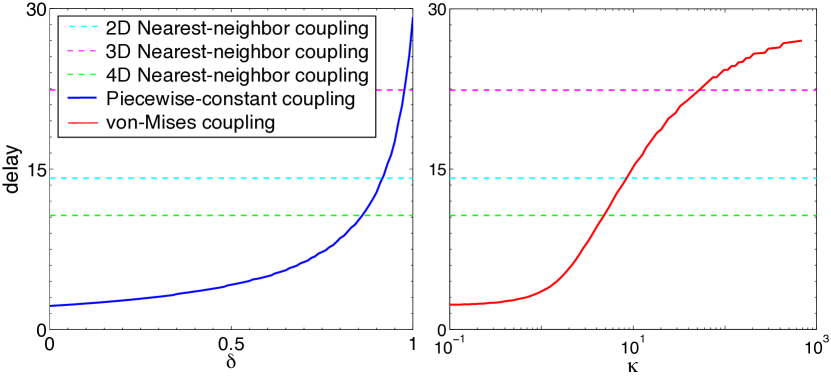
Figure 4: Equilibration time versus perturbation from mean-field coupling. Shown is the simulation time required for the system to evolve from 10% to 90% of the way between its initial condition and the thermalized (zero net magnetization) steady-state. Left panel: piecewise-constant coupling (8); right panel: von Mises coupling (9). Also shown, for reference, is the equilibration time for 2, 3, and 4-dimensional nearest-neighbor coupling (higher dimensions equilibrate faster).

Nearest-Neighbor Coupling—Conventionally, the Ising model couples nearest-neighbor spins arranged on a $d$-dimensional lattice. We can approximate this discrete coupling scheme in a continuous setting by defining our coupling kernel in terms of Dirac delta functions. For one-dimensional nearest-neighbor coupling (periodic), we use:

$$G(\xi,\xi^{\prime})=\frac{1}{2}\left[\delta(\xi-\xi^{\prime}+\epsilon)+\delta(\xi-\xi^{\prime}-\epsilon)\right],$$

where the prefactor is a normalization coefficient and $\epsilon\ll 1$ is analogous to grid spacing in the discrete system. For $H=0$, $T>T_{c}$ and $|s|$ small, Eq. (5) then becomes

$$\dot{s} =\tanh\left[\frac{J}{2kT}\left(s(\xi+\epsilon)+s(\xi-\epsilon)\right)\right]-s$$

$$\approx\tanh\left[\frac{J}{2kT}\left(2s+\epsilon^{2}s_{\xi\xi}\right)\right]-s$$

$$\approx\tanh\left[\frac{Js}{kT}\right]-s+\frac{\epsilon^{2}J}{2kT}s_{\xi\xi}~{}.$$

In general, for $d$-dimensional nearest-neighbor coupling,

$$\dot{s}\approx\tanh\left[\frac{Js}{kT}\right]-s+\frac{\epsilon^{2}J}{2dkT}\nabla^{2}s~{}.$$ (10)

Note that the first two terms of the right-hand side are identical to those in Eq. (6), while the last term can be interpreted as introducing diffusion or smoothing to the system. Thus the nearest-neighbor approach may be approximated by combining uncoupled evolution towards the mean-field steady state and diffusion of magnetization across the system. Figure 5 shows that this approximation works quite well for nearest-neighbor coupling (see Supplemental Material Section S3 for a discussion of the details of this approximation).

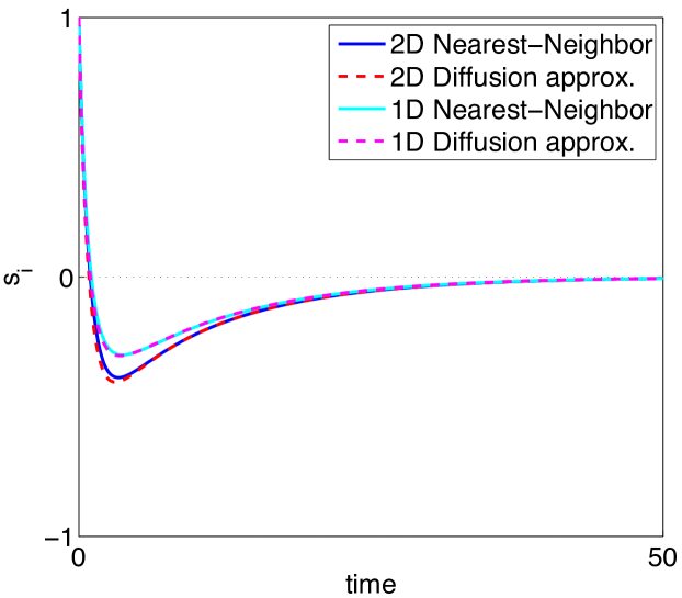
Figure 5: Perturbed spin versus time. To test the approximation to the dynamics in Eq. (10), the system was initialized with a single spin $s_{i}=+1$ while the rest of the system was aligned at $-1$. The time evolution of this misaligned spin is shown for 1D and 2D nearest-neighbor systems together with the diffusive approximation. (The curves in 3D are similar and are omitted for clarity.)

Material Properties—Another advantage of our model is that it allows for straightforward calculation of certain material properties. For example, the magnetic susceptibility $\chi=dm^{*}/dH$ is a measure of how magnetization is influenced by an externally applied field. We may calculate this directly by taking Eq. (6) at steady-state (where $\dot{m}=0$ and $m(t)=m^{*}$) and implicitly differentiating with respect to $H$, resulting in the following expression:

$$\chi=\left\{kT\cosh^{2}\left[\frac{1}{kT}\left(Jm^{*}+H\right)\right]-J\right\}^{-1}~{}.$$

In the limit where $m^{*}\to 0$ and $H\to 0$, we find $\chi\propto(T-J/k)^{-1}$, matching the known result of $\chi\propto(T-T_{c})^{-\gamma}$ with the mean-field value $\gamma=1$ Kadanoff et al. (1967).

For 2D and 3D nearest-neighbor systems, we know from theoretical, numerical, and experimental work that $\gamma>1$ Kadanoff et al. (1967). A drawback to our approach is that the integrodifferential equation (5) cannot give $\gamma\neq 1$ for any smooth coupling kernel. However, an alternative method of gaining insight into this critical exponent may be possible (see Supplemental Material Section S2).

Conclusions—We have taken an unusual approach in our generalization of the Lenz-Ising system via continuum limits in space and spin. Our model discards stochastic fluctuations and therefore precludes the use of many tools of statistical mechanics, but it allows the introduction of a different set of tools typically associated with nonlinear deterministic dynamical systems.

An advantage to our approach is that, once formulated, our model can be analyzed with straightforward calculations that yield fixed points, stability, dynamics, and material properties for arbitrary coupling configurations. The model is amenable to perturbative analysis, allowing for analytical predictions and generating some insight even in cases where exact solution is not possible. For example, with piecewise-constant coupling our model predicts disjoint a equilibrium below a threshold temperature, something that has not been found with the traditional mean-field treatment in statistical mechanics. Because the model is deterministic, a large class of well-explored methods work well in numerical solution.

A disadvantage of this model is that smooth coupling kernels cannot exactly reproduce the behavior of discrete coupling arrangements such as nearest-neighbor. However, it remains unclear whether a smooth approximation to nearest-neighbor coupling may in fact allow for approximation of more complete results such as non-mean-field critical exponents (see Supplemental Material Section S2 for more discussion of this point). Regardless, we believe that this approach to Ising model systems may provide new insight into a long-standing problem.

References

- Domb (1976) C. Domb, in Phase Transitions and Critical Phenomena, Vol. 3, edited by C. Domb and M. Green (Academic Press, New York, 1976) pp. 357–478.
- de Jongh and Miedema (1974) L. J. de Jongh and A. R. Miedema, Advances in Physics 23, 1 (1974).
- Ising (1925) E. Ising, Zeitschrift für Physik A Hadrons and Nuclei 31, 253 (1925).
- Onsager (1944) L. Onsager, Physical Review 65, 117 (1944).
- Stanley (1999) H. E. Stanley, Reviews of modern physics 71, S358 (1999).
- Metropolis et al. (1953) N. Metropolis, A. W. Rosenbluth, M. N. Rosenbluth, A. H. Teller, and E. Teller, The journal of chemical physics 21, 1087 (1953).
- Binder (1976) K. Binder, in Phase Transitions and Critical Phenomena, Vol. 5b, edited by C. Domb and M. Green (Academic Press, New York, 1976) pp. 1–105.
- Abrams et al. (2011) D. M. Abrams, H. A. Yaple, and R. J. Wiener, Physical Review Letters 107, 88701 (2011).
- Glauber (1963) R. J. Glauber, Journal of Mathematical Physics 4, 294 (1963).
- Suzuki and Kubo (1968) M. Suzuki and R. Kubo, J. Phys. Soc. Japan 24, 51 (1968).
- Kadanoff et al. (1967) L. P. Kadanoff, W. Götze, D. Hamblen, R. Hecht, E. Lewis, V. V. Palciauskas, M. Rayl, J. Swift, D. Aspnes, and J. Kane, Reviews of Modern Physics 39, 395 (1967).