Approximation Algorithms for Bayesian Multi-Armed Bandit Problems

Abstract

In this paper, we consider several finite-horizon Bayesian multi-armed bandit problems with side constraints. These constraints include metric switching costs between arms, delayed feedback about observations, concave reward functions over plays, and explore-then-exploit models. These problems do not have any known optimal (or near optimal) algorithms in sub-exponential running time; several of the variants are in fact computationally intractable (NP-Hard). All of these problems violate the exchange property that the reward from the play of an arm is not contingent upon when the arm is played. This separation of scheduling and accounting of the reward is critical to almost all known analysis techniques, and yet it does not hold even in fairly basic and natural setups which we consider here. Standard index policies are suboptimal in these contexts, there has been little analysis of such policies in these settings.

We present a general solution framework that yields constant factor approximation algorithms for all the above variants. Our framework proceeds by formulating a weakly coupled linear programming relaxation, whose solution yields a collection of compact policies whose execution is restricted to a single arm. These single-arm policies are made more structured to ensure polynomial time computability of the relaxation, and their execution is then carefully sequenced so that the resulting global policy is not only feasible, but also yields a constant approximation. We show that the relaxation can be solved using the same techniques as for computing index policies; in fact, the final policies we design are very close to being index policies themselves.

Conceptually, we find policies that satisfy an approximate version of the exchange property, namely, that the reward from a play does not depend on time of play to within a constant factor. However such a property does not hold on a per-play basis and only holds in a global sense: We show that by restricting the state spaces of the arms, we can find single arm policies that can be combined into global (near) index policies that satisfy the approximate version of the exchange property analysis in expectation. The number of different bandit problems that can be addressed by this technique already demonstrate its wide applicability.

1 Introduction.

In this paper, we consider the problem of iterated allocation of resources, when the effectiveness of a resource is uncertain a priori, and we have to make a series of allocation decisions based on past outcomes. Since the seminal contributions of Wald [65] and Robbins [56], a vast literature, including both optimal and near optimal solutions, has been developed, see references in [14, 21, 32].

Of particular interest is the celebrated Multi-Armed Bandit (MAB) problem, where an agent decides on allocating resources between $n$ competing actions (arms) with uncertain rewards and can only take one action at a time (play the arm). The play of the arm provides the agent both with some reward as well as some further information about the arm which causes the state of the arm to be updated. The objective of the agent is to play the arms (according to some specified constraints) for a time horizon $T$ which maximizes sum of the expected rewards obtained in the $T$ steps. The goal of the algorithm designer (and this paper) in this case is to provide the agent with a a decision policy. Formally, each arm $i$ is equipped with a state space ${\cal S}_{i}$ and a decision policy is a mapping from the current states of all the arms to an action, which corresponds to playing a subset of the arms. The goal is to use the description of the state spaces $\{{\cal S}_{i}\}$ and the constraints as input, and output a decision policy which maximizes the objective of the agent. The running time of the algorithm that outputs such a decision policy, and the complexity of specifying the policy itself, should ideally be polynomial in $\sum_{i}|{\cal S}_{i}|$, which is the complexity of specifying the input. In this regard, of particular interest are Index Policies where each arm is reduced to a single priority value and the priority values of the arms (indices) are combined using some scheduling algorithm. Index policies are significantly easier to implement and conceptually reduce the task of designing a decision policy to designing single arm policies. However optimum index policies exist only in limited settings, see [14, 32] for further discussion.

In recent years MAB problems are increasingly being used in situations where the possible alternative actions (arms) are machine generated and therefore the parameter $n$ is significantly large in comparison to the optimization horizon $T$. This is in contrast to the historical development of the MAB literature which mostly considered few alternatives, motivated by applications such as medical treatments or hypothesis testing. While several of those applications considered large $|{\cal S}_{i}|$, many of those results relied on concentration of measure properties derived from the fact that $n/T$ could be assumed to be vanishingly small in those applications.

The recent applications of MAB problems arise in advertising, content delivery, and route selection, where the arms correspond to advertisers, (possibly machine generated) webpages, and (machine generated) routes respectively, and the parameter $n/T$ does not necessarily vanish. As a result, the computational complexity of optimization becomes an issue with large $n$. Moreover, even simple constraints such as budgets on rewards, concavity of rewards render the computation intractable (NP Hard) — and these recent applications are rife with such constraints. This fact forces us to rethink bandit formulations in settings which were assumed to be well understood in the absence of computational complexity considerations. One such general setting is the Bayesian Stochastic Multi-Armed Bandit formulation, which dates back to the results of [7, 18].

Finite Horizon Bayesian Multi-armed Bandit Problem.

We revisit the classical finite-horizon multi-armed bandit problem in the Bayesian setting. This problem forms the basic scaffolding for all the variants we consider in this paper, and is described in detail in Section 2. There is a set of $n$ independent arms. Arm $i$ provides rewards in an $i.i.d.$ fashion based on an parametrized distribution $D_{i}(\theta_{i})$, where the parameter $\theta_{i}$ is unknown. A prior distribution ${\cal D}_{i}$ is specified over possible $\theta_{i}$; the priors of different arms are independent. At each step, the decision policy can play a set of arms (as allowed by the constraints of the specific problem) and observe the outcome of only the set of arms that have been played. Based on the outcomes, the priors of the arms that were played in the previous step are updated using Bayes’ rule to the corresponding posterior distribution. The objective (most often) is to maximize the expected sum of the rewards over the $T$ time steps, where the expectation is taken over the priors as well as the outcome of each play.

The process of updating the prior information for an arm can be succinctly encoded in a natural state space ${\cal S}_{i}$ for arm $i$, where each state encodes the posterior distribution conditioned on a sequence of observations from plays made to that arm. At each state, the available actions (such as plays) update the posterior distribution by Bayes’ rule, causing probabilistic transitions to other states, and yielding a reward from the observation of the play. This process therefore is a special case of the classic finite horizon multi-armed bandit problem [33]. The key property of the state space corresponding to Bayesian updating is that the rewards satisfy the martingale property: The reward at the current state is the same as the expected reward of the distribution over next states when a play is made in that state. The Bayesian MAB formulation is therefore a canonical example of the Martingale Reward Bandit considered in recent literature such as [30].

In this paper, we study several Bayesian MAB variants which are motivated by side-constraints which arise both from modern and historical applications. We briefly outline some of these constraints below, and discuss technical challenges that arise later on.

1. Arms can have budgets on how much reward can be accrued from them - this is a very natural constraint in most applications of the bandit setting.

2. The decision to stop playing an arm can be irrevocable due to high setup costs (or destruction) of the availability of the underlying action.

3. There could be a switching cost from one arm to another; these could be economically motivated and adversarial in nature. These could also arise from feasibility constraints on policies for instance, energy consumption in a sensor network to switch measurements from one node to the next, or for a robot to move physically to a different location.

4. Feedback about rewards can have a time-delay in arriving, for instance in pay-per-conversion auction mechanisms where information about a conversion arrives at a later time. These delays can be non-uniform.

5. The reward at a time-step can be a non-convex function of the set of arms played at that step. Consider for instance, when a person is shown multiple different advertisements, and the sale is attributed to the “most influential” advertisement that was shown; or consider a situation where packets are sent across multiple links (arms) and delivering the packet twice does not give any additional reward.

6. An extreme example of (e) is the futuristic optimization where the the actions taken over the $T$ steps are for exploration only. The goal of the optimization to maximize the reward of the action taken at the $T+1^{st}$ step.

Violation of Exchange Properties.

While the constraints outlined above appear to be very different, they all outline a fundamental issue: They all violate the property that the reward of the arm also does not change depending of when it is scheduled for play. This property of exchange of plays is the most known application of the idling bandit property, which ensures that the state of an arm does not change while that arm is not being played. As a consequence an arm which has high reward on the current play, can be played immediately (“exchanged” with its later play) without any loss of reward. This ability of exchanging plays, is at the core of all existing analysis of stochastic MAB problems with provable guarantees [21, 14, 32]. In fact index policies provide the sharpest example of such an use of the exchangeable property. Contingent on this property, the scheduling decisions can be decoupled from the policy decisions — as a result the optimization problem can be posed without resorting to a “time indexed” formulation.

However this exchangeability of plays does not hold in all the problems we consider here. For example, in constraint (e), the reward is non-convex combination of the outcomes of simultaneous plays of different arms, the reward from the play of an arm is not just the function of the current play of the arm, because the other arms may have larger or smaller values. This is also obviously true if the goal is to maximize the reward of the $T+1^{st}$ step, as in constraint (f). The same issue arises in constraint (d) – the information derived about an arm is not a function of the current play of the arm; since we may be receiving delayed information about that arm due to a previous play. A similar phenomenon occurs in constraints (c) and (b) where conditioned on the decision of switching to another arm, the (effective) reward from an arm changes even though we have not played the arm. For the above problems, the traditional and well understood index policies such as the Gittins index [34, 64] which are optimal for discounted infinite horizon settings, are either undefined or lead to poor performance bounds. Therefore natural questions that arise are: Can we design provably near optimal policies for these problems? Can such policies be shown to be almost (relaxations of) index policies? And perhaps more importantly: What new conceptual analysis idea can we bring to bear on these problems? Answering these questions is the focus of this paper.

1.1 A Solution Recipe

Our main contribution is to present a general solution recipe for all the above constraints. At a high level, our approach uses linear programming of a type that is similar to the widely used weakly coupled relaxation for bandit problems or “decomposable” linear program (LP) relaxation [14, 66]. This LP relaxation provides a collection of single-arm policies whose execution is confined to one bandit arm. Such policies, though not feasible, are desirable for two reasons: First, they are efficient to compute since the computation is restricted to one bandit arm (in contrast, note that the joint state space over all the arms is exponential in $n$); and secondly, they often naturally yield index policies. However, as mentioned before, prior results in this realm crucially require indexability, and fail to provide any guarantees for non-indexable bandit problems of the type we consider. Our recipe below provides a novel avenue for efficiently designing and analyzing feasible policies, albeit at the cost of optimality.

Single-arm Policies:

The first step of the recipe is to consider the execution of a global policy restricted to a single arm, and express its actions only in terms of parameters related to that arm. This defines a single-arm policy. We identify a tractable state space for single arms, which is a function of the original state spaces ${\cal S}_{i}$, and reason that good single arm policies exist in that space. Though classic index policies are constructed using this approach [54, 66], our approach is fundamentally different: In a global policy, actions pertaining to a single arm need not be contiguous in time – our single-arm policies make them contiguous. We show that the martingale property of the rewards enables us to do this step, and this will be the crux of the subsequent algorithm. In essence, though these policies are weaker in structure than previously studied policies, this lack of structure is critical in deriving our results.

Linear Program:

We write a linear programming relaxation, which finds optimal single-arm policies feasible for a small set of coupling constraints across the arms, where the coupling constraints describe how these single arm policies interact within a global policy. This step can either be a direct linear program; however, this is infeasible in many cases, and we show a novel application of the Lagrangian relaxation to not only solve this relaxation, but also analyze the approximation guarantee the relaxation produces.

Scheduling:

The single-arm policies produced by the relaxation are not a feasible global policy. Our final step is to schedule the single arm policies into a globally feasible policy. This scheduling step needs ideas from analysis of approximation algorithms, and specially from the analysis of adaptivity gaps. We note that the feasibility of this step crucially requires the weak structure in the single-arm policies alluded to in the first item. The final policies we design are indeed very similar to (though not the same as) index policies; we highlight this aspect in Section 3.5.

We note that each of the above steps requires new ideas, some of which are problem specific. For instance, for the first step, it is not always obvious why the single-arm policies have polynomial complexity. In constraint (e), the reward depends on the specific set of $K$ arms that are played at any step. This does not correspond naturally to any policy whose execution is restricted to a single arm. Similarly, in constraint (d), the state for a single arm depends on the time steps in the past where plays were made and the policy is awaiting feedback – this is exponential in the length of the delay. Our first contribution is to show that in each case, there are different state space for the policy which has size polynomial in $\sum_{i}|{\cal S}_{i}|,T$, over which we can write a relaxed decision problem.

Similarly, the scheduling part has surprising aspects: For constraint (e), the LP relaxation does not even encode that we receive the max reward every step, and instead only captures the sum of rewards over time steps. Yet, we can schedule the single-arm policies so that the max reward at any step yields a good approximation. For in constraint (d), the single-arm policies wait different amounts of time before playing, and we show how to interleave these plays to obtain good reward.

Finally, there are fundamental roadblocks, above and beyond the specific issues mentioned for each problem, that applies to almost every problem of this genre. There are very few techniques that provide good algorithm-independent upper bounds for these problems. One such approach has been linear programming. But there is a fundamental hurdle regarding the use of linear programs in the context of MAB problems.

A linear program often (and for many of the cases described herein) accounts for the rewards globally after all observations have been revealed. In contrast, a policy typically has to adapt as the observations are revealed. The gap between these two accounting processes is termed as the adaptivity gap (an example of such in the context of scheduling can be found in [25]). The adaptivity gap is a central facet of bandit problems where the policies are adapt to the observable outcomes. We show that there exists policies for whom the adaptivity gap is at most a constant factor! Observe that showing this property also implies satisfying an approximate version of the exchange property, namely, up to a constant factor the reward from a play does not depend on when the play is made. Note that this property does not (can not) hold on a per play basis and is a global statement which holds in expectation.

1.2 Problem Definitions, Results, and Roadmap

We now describe the specific problems we study in this paper, highlighting the algorithmic difficulty that arises therein. In terms of performance bounds, we show that the resulting policies have expected reward which is always within a fixed constant factor of the reward of the optimal policy, regardless of the parameters (such as $n,T$) of the problem, and regardless of the nature of the priors ${\cal D}_{i}$ of the arms. Such a multiplicative guarantee is termed as approximation ratio or factor. We present constant factor approximation algorithms for all the problems we consider. The running times we achieve are small polynomial functions of $T$ and $\sum_{i}|{\cal S}_{i}|$, which is also the complexity of an explicit representation of the state space of each arm. As mentioned above, our running times are very close to the time taken to compute standard indices.

Approximation algorithms are a natural avenue for designing policies, since fairly natural versions of the problems we consider can be shown to be NP-Hard. For instance, for constraint (e), where the per-step reward is the maximum observed value from the set of plays is NP-Hard because it generalizes computing a subset of $k$ distributions that maximizes the expected maximum [35]. The bandit problem with switching costs (constraint c) is Max-SNP Hard since it generalizes an underlying combinatorial optimization problem termed orienteering [17]. For other problems, such as the constraints of irrevocable policies (constraint b), there are examples where no global policy satisfying the said constraint can achieve a reward within a small constant factor of the upper bound proved by some natural linear programming relaxation. In this case, and many others we provide alternate analysis of existing heuristics which have been shown to perform well in practice [30].

We now discuss the specific problems. Each of the problems involve budgets; however, these can be incorporated in the state space in a natural way (by not allowing states corresponding to larger rewards). In some cases, specially constraint (e), budgets pose more unusual challenges.

Irrevocable Policies for Finite Horizon MAB Problem.

This problem was formalized by Farias and Madan [30]. This is the Bayesian MAB problem described earlier where the policy plays at most $K$ arms in a step and the objective is to maximize the expected reward over a horizon of $T$ steps. Each of the arms have budgets on the total reward that can be accrued from that arm. There is an additional constraint that we do not revisit any arm that we have stopped playing. Using the algorithmic framework introduced in [38], Farias and Madan showed an $8$ approximation algorithm which also works well in practice. In Section 3, we provide a better analysis argument (based on revisiting [38] and newer ideas) and that argument improves the result to a factor $(2+\epsilon)$-approximation for any $\epsilon>0$ in time $O((\sum_{i}\mbox{\sc\#Edges}{(}{\cal S}_{i}))\log(nT/\epsilon))$ where $\mbox{\sc\#Edges}{(}{\cal S}_{i})$ is the number of edges that define the statespace ${\cal S}_{i}$. The parameter $\mbox{\sc\#Edges}{(}{\cal S}_{i})$ is a natural representation of the sparsity of the input and thus we can view the algorithm to be almost linear time in that said measure. We also show that $2-O(\frac{1}{n})$ is the best possible bound against weakly coupled relaxations over single arm policies for $n$ arms. Although this is not the main result in this paper, we present this problem first because the intuitive analysis idea is used throughout the paper and this problem has a right level of complexity for illustrative purposes.

Traversal Dependent MAB Problems.

It is widely acknowledged [12, 19] that the scenarios that call for the application of bandit problems typically have constraints/costs for switching arms. Banks and Sundaram [12] provide an illuminating discussion even for the discounted reward version, and highlight the technical difficulty in designing reasonable policies. Since the switching costs couple the arms together, it is not even clear how to define a weakly coupled system. These constraints/costs can be motivated by strategic considerations and even be adversarial: Price-setting under demand uncertainty [57], decision making in labor markets [47, 53, 12], and resource allocation among competing projects [11, 32]. For instance [12, 11], consider a worker who has a choice of working in $k$ firms. A priori, she has no idea of her productivity in each firm. In each time period, her wage at the current firm is an indicator of her productivity there, and partially resolves the uncertainty in the latter quantity. Her expected wage in the period, in turn, depends on the underlying (unknown) productivity value. At the end of each time step, she can change firms in order to estimate her productivity at different places. Her payoff every epoch is her wage at the firm she is employed in at that epoch. The added twist is that changing firms does not come for free, and incurs a cost to the worker. What should the strategy of the worker be to maximize her (expected) payoff? A similar problem can be formulated from the perspective of a firm trying out different workers with a priori unknown productivity to fill a post. On the other hand, the switching costs may be constraints imposed on the policies by physical considerations – for example an energy constrained robot moving to specific locations. The above discussion suggests two sets of problems – the Adversarial Order Irrevocable Policies for Finite Horizon MAB problem and the MAB with Metric Switching Costs problem. We address each of them below:

Adversarial Order Irrevocable Policies for Finite Horizon MAB.

In all these cases, the decision agent may not have the flexibility to choose an ordering of events and yet have to provide some algorithm with provable rewards. In this problem we are asked to design a collection of single arm policies subject to a total horizon of $T$ and $K$ plays at a time. After we design the policies, an adversary chooses the order in which we can play the arms irrevocably – if we quit playing an arm then we cannot return to playing that same arm. We then schedule the policies such that we maximize the expected reward. This problem naturally models a “switching cost” behavior where the costs are induced by an adversary. To the best of our knowledge this problem had not been formulated earlier – in Section 4 we provide a $(4+\epsilon)$-approximate solution (when compared to the best possible order we could have received) that can be computed in time $O((\sum_{i}\mbox{\sc\#Edges}{(}{\cal S}_{i}))\log(nT/\epsilon))$ as before. The main benefit of this problem is revealed in the next problem on metric switching costs.

MAB with Metric Switching Costs.

In this variant, the arms are located in a metric space with distance function $\ell$. If the previous play was for arm $i$ and the next play is for arm $j$, the distance cost incurred is $\ell_{ij}$. The total distance cost is at most $L$ in all decision paths. The policy pays this cost whenever it switches the arm being played. If the budget $L$ is exhausted, the policy must stop. This problem already models the more common “switching in-and-out” costs using a star graph. To the best of our knowledge there was no prior theoretical results on the Bayesian multi-armed bandit with metric switching costs. Observe that in absence of the metric assumption, the problem already encodes significantly difficult graph traversal problems and are unlikely to have bounded performance guarantees. In Section 4, we present a $(4+\epsilon)$-approximation (for any $\epsilon>0$) the Finite-horizon MAB problem with metric switching costs for $K=1$. The result worsens to $(4.5+\epsilon)$-approximation for any $K\geq 2$. This result uses the ideas from the adversarially ordered bandits and separates the hard combinatorial traversal decisions from the bandit decisions.

Delayed Feedback.

In this variant, the feedback about a play (the observed reward) for arm $i$ is obtained after some $\delta_{i}$ time steps. This notion was introduced by Anderson [5] in an early work in mid 1960s. Since then, though there have been additional results [62, 23], a theoretical guarantee on adaptive decision making under delayed observations has been elusive, and the computational difficulty in obtaining such has been commented upon in [27, 6, 59, 28]. Recently, this issue of delays has been thrust to the fore due to the increasing application of iterative allocation problems in online advertising. As an example described in Agarwal etal in [2], consider the problem of presenting different websites/snippets to an user and induce the user to visit these web pages. Each pair of user and webpage define an arm. The delay can also arise from batched updates and systems issues, for instance in information gathering and polling [2], adaptive query processing [63], experiment driven management and profiling [10, 45], reflective control in cloud services [26], or unmanned aerial vehicles [55]. There has been little formal analysis of delayed feedback and its impact on performance despite the fact that delays are ubiquitous.

We note that in the case of delayed feedback, even for a single arm, the decision policy needs to keep track of plays with outstanding feedback for that arm, so that the optimal single-arm decision policy has complexity which is exponential in the delay parameter $\delta_{i}$. It is therefore not clear how to solve the natural weakly coupled LP efficiently. In a broader sense, the challenge in the delayed setting is not just to balance explorations along with the exploitation, but also to decide a schedule for the possible actions both for a single arm (due to delays) as well as across the arms. In Section 5, we show several constant factor approximations for this problem. We show that when $\max_{i}\delta_{i}\leq\sqrt{T}/50$ then the approximation ratio does not exceed $3$ even for playing $K$ different arms (with additive rewards) simultaneously. The approximation ratio worsens but remains $O(1)$ for $\max_{i}\delta_{i}\leq T/(48\log T)$. Interestingly the policies obtained from these algorithm satisfy the property for each single arm which is best summarized as: “quit, exploit or double the exploration” which is a natural policy in retrospect. Moreover the different algorithmic approaches expose the natural “regimes” of the delay parameter from small to large.

Non-Convex Reward Functions.

Typically, MAB problems have focused on either the reward from the played arm, or if multiple arms are played, the sum of the rewards of these arms. However, in many applications, the reward from playing multiple arms is some concave function of the individual rewards. Consider for instance charging advertisers based on tracking clicks made by a user before they make a conversion; in this context, the charge is made to the most influential advertiser on this path and is hence a non-linear function of the clicks made by the user. As another example, consider an fault tolerant network application wishing to choose send packets along $K$ independent routes [3]. The network only has prior historical information about the success rate of each of the routes and wishes to simultaneously explore the present status of the routes as well as maximize the probability of delivery of the packet. This problem can be modeled as a multi-armed bandit problem where multiple arms are being played at a time step and the reward is a nonlinear (but concave) function of the rewards of the played arms. As a concrete example, we define the MaxMAB problem, where at most $K$ arms can be played every step, and the reward at any step is the maximum of the observed values. This problem produces two interesting issues:

First, if only the maximum value is obtained as a reward, should the budgets of the other arms be decreased? A case can be made for either an answer of “yes” (budgets indicate opportunity) which defines a All-Plays-Cost accounting or an answer of “no” (budgets indicate payouts of competing advertisers in a repeated bidding scenario) which defines Only-Max-Costs accounting.

Second, if multiple arms are played and their rewards are non-additive, does the modeling of how the feedback is received (One-at-a-Time or Simultaneous-Feedback) affect us? In Section 6, we provide a $(4+\epsilon)$-approximation in the model where the budgets of all arms are decreased and the feedback is received one-at-a-time. We also show that these four variants (from the two issues) are related to each other and their respective optimum solutions do not differ by more than a $O(1)$ factor. We show this by providing algorithms in a weaker model that achieve $O(1)$ factor reward of the optimum in a correspondingly stronger model. From a policy perspective, the policies designed for this problem have the property that restricted to a single arm, the differences between small reward outcomes are ignored. Therefore the policy focuses on an almost index-like computation of only the large reward outcomes.

Future Utilization and Budgeted Learning.

One of the more recent applications of MAB has been the Budgeted Learning type applications popularized by [50, 52, 58]. This application has also been hinted at in [7]. The goal of a policy here is to perform pure exploration for $T$ steps. At the $T+1^{st}$ step, the policy switches to pure exploitation and therefore the objective is to optimize the reward for the $T+1^{st}$ step. The simplest example of such an objective is to choose one arm so as to maximize the (conditional) expected value; more formally, given any policy $\pi$ we have a probability distribution over final (joint) state space. In each such (joint) state, the policy chooses the arm that maximizes the expected value – observe that this is a function $g(\pi)$ of the chosen policy. The goal is to find the policy that maximizes the expected value of $g(\pi)$ where the expectation is taken over all initial conditions and the outcomes of each play. Note that the non-linearity arises from the fact that different evolution paths correspond to different final choices. Natural extensions of such correspond to Knapsack type constraints and similar problems have been discussed in the context of power allocation (when the arms are channels) [24] and optimizing “TCP friendly” network utility functions [51]. In Section 7 we provide a $(3+\epsilon)$-approximation for the basic variant.

1.3 Related Work

Multi-armed bandit problems have been extensively studied since their introduction by Robbins in [56]. From that starting point the literature has diverged into a number of (often incomparable) directions, based on the objective and the information available. In context of theoretical results, one typical goal [49, 8, 21, 60, 61, 20, 48, 31] has been to assume that the agent has absolutely no knowledge of $\rho_{i}$ (model free assumption) and then the task has been to minimize the “regret” or the lost reward, that is comparing the performance to an omniscient policy that plays the best arm from the start. However, these results both require the reward rate to be large and large time horizon $T$ compared the number of arms (that is, vanishing $n/T$). In the application scenarios mentioned above, it will typically be the case that the number of arms is very large and comparable to the optimization horizon and the reward rates are low.

Moreover almost all analysis of stochastic MAB in the literature has relied on the exchange property; these results depend on “moving plays/exchange arguments” — if we can play arm $i$ currently, we consider waiting or moving the play of the arm to a later time step without any loss. The exchange properties are required for defining submodularity as well as its extensions, such as sequence or adaptive submodularity [60, 37, 4]. The exchange property is not true in cases of irrevocability (since we cannot have a gap in the plays, so moving even a single play later creates a gap and is infeasible), delays (since if the next play of an arm is contingent on the outcome of the previous play, we cannot move the first play later arbitrarily because then we may make the second play before the outcome of the the first is known, which is now infeasible), or non-linear rewards (since the reward is explicitly dependent on the subset of plays made together). It may be appear that we can avoid the issue by appealing to non-stochastic/adversarial MABs [9] – but they do not help in the presence of budget constraints which couples the action across various time steps. It is known that online convex analysis cannot be analyzed well in the presence of large number of arms and a “state” that couples the time steps [29]. Budgets are one of the ways a “state” is enforced. Delays and irrevocability also explicitly encode state. All future utilization objectives trivially encode state as well.

The problem considered in [61] is similar in name but is different from the MaxMAB problem we have posed herein — that paper maximizes the single maximum value seen across all the arms and across all the $T$ steps. The authors of [36] show that several natural index policies for the budgeted learning problem are constant approximations using analysis arguments which are different from those presented here. The specific approximation ratios proved in [36] are improved upon by the results herein with better running times. The authors of [44] present a constant approximation for non-martingale finite horizon bandits; however, these problems require techniques that are orthogonal to those in this paper. The problems considered in [43] is an infinite horizon restless bandit problem. Though that work also uses a weakly coupled relaxation and its Lagrangian (as is standard for many MAB problems), the techniques we use here are different.

2 Preliminaries: State Spaces, Budgets and Decision Policies

Recall the basic setting of the finite horizon Bayesian MAB problem. There is a set of $n$ independent arms. Arm $i$ provides rewards in an $i.i.d.$ fashion from a parametrized distribution $D_{i}(\theta_{i})$. The parameter $\theta_{i}$ can be arbitrary. It is unknown at the outset, but a prior ${\cal D}_{i}$ is specified over possible values of $\theta_{i}$. The priors of different arms are independent. At each step, a decision policy can play a set of arms (as allowed by the constraints of the specific problem) and observe the outcome of only the set of arms that have been played. Based on the outcomes, the priors $\{{\cal D}_{i}\}$ of the arms that were played in the previous step are updated using Bayes’ rule to the corresponding posterior distributions. The objective of the decision policy (most often) is to maximize the expected sum of the rewards obtained over the $T$ time steps, where the expectation is taken over the priors as well as the outcome of each play. We note that other objectives are possible; we also consider the case where the $T$ plays are used for pure exploration, and the goal is to optimize the expected reward for the $T+1^{st}$ play.

2.1 State Space of an Arm and Martingale Rewards

Let $\sigma$ denote a sequence of observed rewards, when $k=|\sigma|$ plays of arm $i$ are made. Given these observations, the prior ${\cal D}_{i}$ uniquely updates to a posterior ${\cal D}_{i\sigma}$. Since the rewards are $i.i.d.$, only the set (as opposed to sequence) of observations $\sigma$ matters in uniquely defining the posterior distribution. Suppose $D_{i}(\theta)$ is a $r$ valued distribution, a sequence of $k$ plays can therefore yield ${r+k\choose k}$ sets $\sigma$. Each of these uniquely defines a posterior distribution ${\cal D}_{i\sigma}$. We term each of these sets $\sigma$ as a state of arm $i$. At any point in time, the arm $i$ is in some state, and over a horizon of $T$ steps, the number of possible states is $O(T^{r})$. We denote the set of these states as ${\cal S}_{i}$, and a generic state as $u\in{\cal S}_{i}$. Let the start state corresponding to the initial prior ${\cal D}_{i}$ be denoted $\rho_{i}$.

Given a posterior distribution ${\cal D}$ of arm $i$ (corresponding to some state $u\in{\cal S}_{i}$ and set of observations $\sigma$), the next play can be viewed as follows: A parameter $\theta_{i}$ is drawn from ${\cal D}$, and a reward is observed from distribution $D_{i}(\theta_{i})$. Therefore, the posterior distribution ${\cal D}$ at state $u$ also defines the distribution over observed rewards of the next play. If the observed reward is $q$, this modifies the state from $u$ with set of observations $\sigma$ to state $v$ corresponding to the set $\sigma\cup\{q\}$. We define $\mathbf{p}_{uv}$ as the probability of this event conditioned on being at state $u$ and executing a play.

We further define $r_{u}=\mathbf{E}[D_{i}(\theta)|{\cal S}_{i}=u]$ as the expected value of the observed reward of this play. We term this the reward of state $u$. Let $\mbox{\sc\#Edges}{(}{\cal S}_{i})$ be the number of non-zero transition edges in ${\cal S}_{i}$, i.e., $\mathbf{p}_{uv}\neq 0$. We use the notation $|{\cal S}_{i}|$ to denote the number of states and if the play in each state has at most $d$ outcomes then $\mbox{\sc\#Edges}{(}{\cal S}_{i})\leq d|{\cal S}_{i}|\leq|{\cal S}_{i}|^{2}$. Observe that $\sum_{i}\mbox{\sc\#Edges}{(}{\cal S}_{i})$ is a natural measure of input sparsity.

Compact Representation and Martingale Property.

At this point, we can forget about Bayesian updating (for the most part), and pretend we have a state space ${\cal S}_{i}$ for arm $i$, where state $u$ yields reward $r_{u}$, and has transition probability matrix $\{\mathbf{p}_{uv}\}$. The goal is to design a decision policy for playing the arms (subject to problem constraints) so that the expected reward over $T$ steps is maximized. Since the prior updates satisfy Bayes’ rule, it is a standard observation that $r_{u}=\sum_{v\in{\cal S}_{i}}\mathbf{p}_{uv}r_{v}$ for all states $u\in{\cal S}_{i}$. In other words, the state space of an arm satisfies the Martingale property on the rewards. We note that all our results except for the one in Section 5 hold for arbitrary state spaces satisfying the martingale property; however, we choose to present the results for case of Bayesian updates, since this is the canonical and most widely known application of the MAB problems.

Example: Bernoulli Bandits.

Consider a fixed but unknown distribution over two outcomes (success or failure of treatment, click or no click, conversion or no conversion). This is a Bernoulli$(1,\theta)$ trial where $\theta$ is unknown. A family of prior distribution on $\theta$ is the Beta distribution; this is the conjugate prior of the Bernoulli distribution, meaning that the posterior distributions also lie within the same family. A Beta distribution with parameters $\alpha_{0},\alpha_{1}\in\mathbb{Z}^{+}$, which we denote $Beta(\alpha_{1},\alpha_{0})$ has p.d.f. of the form $c\theta^{\alpha_{1}-1}(1-\theta)^{\alpha_{0}-1}$, where $c$ is a normalizing constant. $Beta(1,1)$ is the uniform distribution. The distribution $Beta(\alpha_{1},\alpha_{0})$ corresponds to the current (posterior) distribution over the possible values of $\theta$ after having observed $(\alpha_{1}-1)$ $1$’s and $(\alpha_{0}-1)$ $0$’s, starting from the belief that $\theta$ was uniform, distributed as $Beta(1,1)$.

Given the distribution $u=Beta(\alpha_{1},\alpha_{0})$ as the prior, the expected value of $\theta$ is $\mu_{u}=\frac{\alpha_{1}}{\alpha_{1}+\alpha_{0}}$, and this is also the expected value of the observed outcome of a play conditioned on this prior. Updating the prior on a sample is straightforward. On seeing a $1$, the posterior (of the current sample, and the prior for the next sample) is $v=Beta(\alpha_{1}+1,\alpha_{0})$, and this event happens with probability $\mu_{u}$. On seeing a $0$, the new distribution is $w=Beta(\alpha_{1},\alpha_{0}+1)$ and this event happens with probability $1-\mu_{u}$.

The posterior density $u=Beta(\alpha_{1},\alpha_{0})$ corresponds to state $u\in{\cal S}_{i}$, and can be uniquely specified by the values $(\alpha_{1},\alpha_{0})$. Therefore, $r_{u}=\mu_{u}$. If the arm is played in this state, the state evolves to $v$ with probability $\mathbf{p}_{uv}=\mu_{u}$ and to $w$ with probability $\mathbf{p}_{uw}=1-\mu_{u}$. As stated earlier, the hard case for our algorithms (and the case that is typical in practice) is when the input to the problem is a set of arms $\{i\}$ with priors ${\cal D}_{i}\sim Beta(\alpha_{1i},\alpha_{0i})$ where $\alpha_{0i}\gg\alpha_{1i}$ which corresponds to a set of poor prior expectations of the arms. Observe that $\mbox{\sc\#Edges}{(}{\cal S}_{i})\leq 2|{\cal S}_{i}|$ for this example.

2.2 Modeling Budgets and Feedback

One ingredient in our problem formulations is natural budget constraints in individual arms. As we will see later, these constraints introduce non-trivial complications in designing the decision policies. There are three types of budget constraints we can consider.

Play Budget Model:

This corresponds to the number of times an individual arm $i$ can be played, typically denoted by $T_{i}$ where $T_{i}\leq T$. In networking, each play attempts to add traffic to a route and we may choose to avoid congestion. In online advertising, we could limit the number of impressions of a particular advertisement, often done to limit advertisement-blindness.

All-Plays-Cost Model

The total reward obtained from arm $i$ should be at most its budget $B_{i}$. The arm can be played further, but these plays do not yield reward.

Only-Max-Costs Model

In MaxMab, the reward of only the arm that is maximum is used, and hence only this budget is depleted. In other words, there is a bound on the total reward achievable from an arm (call this $A_{i}$), but we only count reward from an arm when it was the maximum value arm at any step.

Observe that the play budget and All-Plays-Cost models simply involve truncating the state space ${\cal S}_{i}$, so that an arm cannot be played if the number of plays or observations violates the budget constraint – this obviates the need to discuss this constraint explicitly in most sections. The Only-Max-Costs model is more complicated to handle, requiring expanding the state space to incorporate the depleted budget. We discuss that model only in Section 6.4. Note however that the All-Plays-Cost model is also nontrivial to encode in the context of delays in feedback, and we discuss that model in Section 5 further.

Modeling the feedback received is an equally important issue. We just alluded to delays in the feedback for the play of a single arm. However if multiple plays are being made simultaneously – the definition of simultaneity has interesting consequences. We can conceive two models:

One-at-a-Time Feedback:

In this model even if we are allowed to play $K>1$ arms in a single time slot, we make only one play a time and receive the feedback before making the play of a different arm in that same time slot.

Simultaneous-Feedback:

In this model we decide on a palette of at most $K$ plays in a time slot and make them before receiving the result of any of the plays in that time slot.

Clearly, the One-at-a-Time model allows for more adaptive policies. However for additive rewards, where we sum up the rewards obtained from all the plays made in a time slot – this issue regarding the order of feedback is not very relevant. However in the case where we have subadditive rewards then the distinction between One-at-a-Time and Simultaneous-Feedback is clearly significant – specially in the All-Plays-Cost accounting. The distinction continues to hold in the Only-Max-Costs pays model as well, because we can adapt the set of arms to play to the outcome of the initial plays in the same time slot.

2.3 Decision Policies and Running Times

A decision policy ${\cal P}$ is a mapping from the current state of the overall system to an action, which involves playing $K$ arms in the basic version of the problem. This action set can be richer, as we discuss in subsequent sections. Observe that the state of the overall system involves all the knowledge available to the policy, including:

1. The joint states $\{u\in{\cal S}_{i}\}$ of all the arms;

2. The current time step, which also yields the remaining time horizon;

3. The remaining budget of all the arms;

4. Plays made in the past for which feedback is outstanding (in the context of delayed feedback).

Therefore, the “state” used by a decision policy could be much more complicated than the product space of ${\cal S}_{i}$, and one of our contributions in this paper is to simplify that state space and make it tractable.

Running Times.

Our goal will be to compute decision policies in time that depends polynomially on $T$ and $\sum_{i}|{\cal S}_{i}|$, which is the sum of the sizes of the state spaces of all the arms. In the case of Bernoulli bandits discussed above, this would be polynomial in the number of arms $n$, and the time horizon $T$. Our running times and the description of the final policies will be comparable (in a favorable way) to the time required for dynamic programming to compute the standard index policies [14, 34]. This will become clear in Section 3; however, fine-tuning the running time is not the main focus of this paper. However our running times will often be linear in the natural input sparsity, that is, $\sum_{i}\mbox{\sc\#Edges}{(}{\cal S}_{i})$.

2.3.1 Single Arm Policies

A single arm policy $P_{i}$ for arm $i$ is a policy whose execution (actions and rewards) are only confined to the state space of arm $i$. In other words, it has one of several possible actions at any step; in the basic version of the problem, the available actions at any step involve either (i) play the arm – if the arm is in state $u\in{\cal S}_{i}$, this yields reward $r_{u}$; or (ii) stop playing and exit. Furthermore, the actions of $P_{i}$ only depend on the state variables restricted to arm $i$ – the current state $u\in{\cal S}_{i}$, remaining budget of arm $i$, the remaining time horizon, etc. In most situations we will eliminate states that cannot be reached in $T$ steps (the horizon). Formally;

Definition 1.

Let ${\cal S}_{i}(T)$ be the state space ${\cal S}_{i}$ truncated to $T$ steps. Let ${\mathcal{C}}_{i}(T)$ describe all single-arm policies of arm $i$ with horizon $T$. Each $P_{i}\in{\mathcal{C}}_{i}(T)$ is a (randomized) mapping from the current state of the arm to an action. The state of the system is captured by the current posterior $u\in{\cal S}_{i}(T)$ and the remaining time horizon. Such a policy at any point in time has at two available actions: (i) Play the arm; or (ii) stop. Note that the states and actions are for the basic problem, so that variants will have more states/actions which will be described at the appropriate context.

Definition 2.

Given a single-arm policy $P_{i}$ let $R(P_{i})$ to be the expected reward and $\mathcal{T}(P_{i})$ as the expected number of plays made. The expectation is taken over all randomizations within the policy as well as all outcomes of all plays.

The construction of single-arm policies will be non-trivial, as will be described in subsequent sections. One of the contributions of this paper is in the development of single-arm policies with succinct descriptions. Succinct descriptions also allow us to focus on key aspects of the policy and analyze simple and common modifications of the policies.

3 Irrevocable Policies for Finite Horizon Bayesian MAB Problems

In this section we consider the basic finite horizon Bayesian MAB problem (as defined in Section 1) with the additional constraint of Irrevocability; that is, the plays for any arm are contiguous. Recently, Farias and Madan [30] provided an $8$-approximation for this problem. Previously, constant factor approximations were provided in [36, 40] for the finite horizon MAB problem (not necessarily using irrevocable policies). The analysis herein provides a significant strengthening of all previous results on this problem. The contribution of this section is the introduction of a palette of basic techniques which are illustrative of all the (significantly more difficult) problems in this paper.

In term of specific results we show that given a solution of the standard LP formulation for this problem, a simple scheduling algorithm provides a $2$ approximation (Theorem 4). Moreover we prove that this is the best possible result against the standard LP solution. We then show that we can compute a near optimal solution of the standard LP efficiently, that is, for any $\epsilon\in(0,1]$ we provide an algorithm that runs in $O((\sum_{i}\mbox{\sc\#Edges}{(}{\cal S}_{i}))\log(nT/\epsilon))$ time and provides a $2+\epsilon$-approximate solution against the optimum solution of that standard LP (Theorem 7 and Corollary 8).

In terms of techniques we introduce a compact LP representation and its analysis based on Lagrangians, which are used throughout the rest of the paper. Likewise we consider the technique of truncation in Section 3.2 – while this technique is similar to [30, Lemma 2] but our presentation uses a slightly different intuition that is also useful throughout this paper.

Roadmap:

We present the standard LP relaxation that bounds the value of the optimum solution $OPT$ in Section 3.1; along with an interpretation of fractional solution of that LP in terms of single arm policies. We show how the standard LP can be represented in a compact form demonstrating the weak coupling. As stated, we discussion truncation in Section 3.2. In Section 3.3 we then present the $2$-approximation result (Theorem 4) and the (family of) examples which demonstrate that the bound of $2$ is tight. In Section 3.4 we then show how to achieve the $(1+\epsilon)$-approximation (Theorem 7 and Corollary 8) for the compact LP. We conclude in Section 3.5 with a comparison between the Lagrangian induced solutions and the Gittins Index.

3.1 Linear Programming Relaxations and Single arm Policies

Consider the following LP, which has two variables $w_{u}$ and $z_{u}$ for each arm $i$ and each $u\in{\cal S}_{i}(T)$. Recall ${\cal S}_{i}(T)$ is the statespace ${\cal S}_{i}$ truncated to a horizon of $T$ steps. The variable $w_{u}$ corresponds to the probability (over all randomized decisions made by any algorithm as well as the random outcomes of all plays made by the same algorithm) that during the execution of arm $i$ enters state $u\in{\cal S}_{i}$. Variable $z_{u}$ corresponds to the probability of playing arm $i$ in state $u$.

$$\begin{array}[]{rcll}\displaystyle\mbox{\sc LP1}&=&\displaystyle\mbox{Max}\sum_{i=1}^{n}\sum_{u\in{\cal S}_{i}(T)}r_{u}z_{u}&\\ \sum_{i=1}^{n}\sum_{u\in{\cal S}_{i}}z_{u}&\leq&KT&\\ \sum_{v\in{\cal S}_{i}}z_{v}\mathbf{p}_{vu}&=&w_{u}&\forall i,u\in{\cal S}_{i}(T)\setminus\{\rho_{i}\}\\ z_{u}&\leq&w_{u}&\forall u\in{\cal S}_{i}(T),\forall i\\ z_{u},w_{u}&\in&[0,1]&\forall u\in{\cal S}_{i}(T),\forall i\\ \end{array}$$

We use LP1 to refer to the value and (LP1) as the LP.

Claim 1.

Let $OPT$ be the value of the optimum policy. Then $OPT\leq\mbox{\sc LP1}$.

Proof.

We show that the $\{w^{*}_{u},z^{*}_{u}\}$ as defined above, corresponding to a globally optimal policy ${\cal P}^{*}$, are feasible for the constraints of the LP.

The first constraint follows by linearity of expectation: The expected time for which arm $i$ is played by ${\cal P}^{*}$ is $T_{i}=\sum_{u\in{\cal S}_{i}(T)}z^{*}_{u}$. Since at most $K$ arms are played every step, we must have $\sum_{i}T_{i}\leq KT$, which is the first constraint. Note that $T_{i}\leq T$, since we have truncated ${\cal S}_{i}$ to have only states corresponding to at most $T$ observations.

The second constraint simply encodes that the probability of reaching a state $u\in{\cal S}_{i}(T)$ precisely the probability with which it is played in some state $v\in{\cal S}_{i}(T)$, times the probability $\mathbf{p}_{vu}$ that it reaches $u$ conditioned on that play. The constraint $z_{u}\leq w_{u}$ simply captures that the event an arm is played in state $u\in{\cal S}_{i}(T)$ only happens if the arm reaches this state.

The objective is precisely the expected reward of the optimal policy – recall that the reward of playing arm $i$ in state $u$ is $r_{u}$. Hence, the LP is a relaxation of the optimal policy. ∎

A similar LP formulation was proposed for the multi-armed bandit problem by Whittle [66] and Bertsimas and Nino-Mora [54]; however, one key difference is that we ignore the time at which the arm is played in defining the LP variables.

From Linear Programs to Single Arm Policies:

The optimal solution to (LP1) clearly does not directly correspond to a feasible policy since the variables do not faithfully capture the joint evolution of the states of different arms – in particular, the optimum solution to (LP1) enforces the horizon $T$ only in expectation over all decision paths, and not individually on each decision path. In this paper, we present such relaxations for each variant we consider, and develop techniques to solve the relaxation and convert the solution to a feasible policy while preserving a large fraction of the reward. Below, we present an interpretation of any feasible solution to (LP1), which also helps us compact representation subsequently.

Let $\langle w_{u},x_{u},z_{u}\rangle$ denote any feasible solution to the (LP1). Assume w.l.o.g. that $w_{\rho_{i}}=1$ for all $i$. Ignoring the first constraint of (LP1) for the time being, the remaining constraints encode a separate policy ${\cal P}_{i}$ for each arm as follows: Consider any arm $i$ in isolation. The play starts at state $\rho_{i}$. The arm is played with probability $z_{\rho_{i}}$, so that state $u\in{\cal S}_{i}(T)$ is reached with probability $z_{\rho_{i}}\mathbf{p}_{\rho_{i}u}$. Similarly, conditioned on reaching state $u\in{\cal S}_{i}(T)$, with probability $z_{u}/w_{u}$, arm $i$ is played. This yields a policy ${\cal P}_{i}$ for arm $i$ which is described in Figure 1.

Policy ${\cal P}_{i}$: If arm $i$ is currently in state $u$, then choose $q\in[0,w_{u}]$ uniformly at random: 1. If $q\in[0,z_{u}]$, then play the arm. 2. If $q\in(z_{u},w_{u}]$, then stop executing ${\cal P}_{i}$.

Figure 1: The Policy ${\cal P}_{i}$.

For policy $P_{i}$, it is easy to see by induction that if state $u\in{\cal S}_{i}(T)$ is reached by the policy with probability $w_{u}$, then state $u\in{\cal S}_{i}(T)$ is reached and arm $i$ is played with probability $z_{u}$. Therefore, $P_{i}$ satisfies all the constraints of (LP1) except the first. The first constraint simply encodes that the total expected number of plays made by all these single-arm policies $\{P_{i}\}$ is at most $KT$.

Note that any feasible solution of (LP1) defines a collection of single arm policies $\{{\cal P}_{i}\}$ and each ${\cal P}_{i}\in{\mathcal{C}}_{i}(T)$ as defined in Definition 1. Using the notation in Definition 2, $R(P_{i})=\sum_{u\in{\cal S}_{i}(T)}r_{u}z_{u}$ and $\mathcal{T}(P_{i})=\sum_{u\in{\cal S}_{i}(T)}z_{u}$ we can represent (LP1) as follows:

$$\mbox{\sc LP1}=\mbox{Max}_{\{P_{i}\in{\mathcal{C}}_{i}(T)\}}\left\{\sum_{i}R(P_{i})\ |\ \sum_{i}\mathcal{T}(P_{i})\leq KT\right\}$$

3.2 The Idea of Truncation

We now show that the time horizon of a single-arm policy on $T$ steps can be reduced to $\beta T$ for constant $\beta\leq 1$ while sacrificing a constant factor in the reward. We note that though the statement seems simple, this theorem only applies to single-arm policies and is not true for the global policy executing over multiple arms. The proof of this theorem uses the martingale structure of the rewards, and proceeds via a stopping time argument. A similar statement is proved in [30, Lemma 2] using an inductive argument; however that exact proof would require modifications in the varied setting we are applying it and therefore we restate and prove the theorem.

Definition 3.

Given a policy ${\cal P}$, a decision path is a sequence of (observed reward, action) pairs encountered by the policy till stopping. Different decision paths are encountered by the policy with different probabilities, which depend on the observed rewards.

Recall the notation $R({\cal P}),\mathcal{T}({\cal P})$ introduced in Definition 2.

Theorem 2.

(The Truncation Theorem.) Consider an arbitrary single arm policy ${\cal P}$ executing over state space ${\cal S}$ defined by $i.i.d.$ draws from a reward distribution $D(\theta)$, where a prior distribution ${\cal D}$ is specified over the unknown parameter $\theta$. Suppose $\mathbf{E}[D(\theta)]\geq 0$ for all parameter choices $\theta$. Consider a different policy ${\cal P}^{\prime}$ that executes the decisions of ${\cal P}$ but stops after making (at least) $\beta$ fraction of the plays on any decision path of ${\cal P}$. Then (i) $R({\cal P}^{\prime})\geq\beta R({\cal P})$ and (ii) $\mathcal{T}({\cal P}^{\prime})\leq\mathcal{T}({\cal P})$.

Proof.

We view the system as follows. The unknown reward distribution $D(\theta)$ has mean $\mu(\theta)$, and the initial prior ${\cal D}$ over $\theta$ specifies a prior distribution $f(\mu)$ over possible $\mu$. Consider the execution of ${\cal P}$ conditioned on the event that the (unknown) mean is $\mu$, and denote this execution as ${\cal P}(\mu)$. Let $R({\cal P}(\mu)),\mathcal{T}({\cal P}(\mu))$ denote the expected reward and the number of plays of the policy ${\cal P}$ conditioned on this event. We have $R({\cal P})=\int R({\cal P}(\mu))f(\mu)d\mu$ and $\mathcal{T}({\cal P})=\int\mathcal{T}({\cal P}(\mu))f(\mu)d\mu$.

Suppose the execution ${\cal P}(\mu)$ reaches some state $v\in{\cal S}$ on decision path $q$ and decides to make a play there. Since the rewards are $i.i.d.$ draws, the expected reward of the next play at $v$ is $\mu$ regardless of the state. We charge the reward to the path $q$ as follows: Regardless of the actual observation at state $v$ corresponding to path $q$, we charge reward exactly equal to $\mu$ to $q$ for making a play at state $v$. In other terms, we charge reward exactly $\mu$ whenever a play is made is any state, regardless of the actual observation. It is clear that the expected reward of any play is preserved by this accounting scheme, since the rewards are $i.i.d.$ draws from a distribution with mean $\mu$.

By linearity of expectation, the above charging scheme means that for any decision path $q$, the expected reward is simply $\mu$ times the number of plays made on this path. More formally, suppose decision path $q$ involves $l(q)$ plays and that is taken by ${\cal P}(\mu)$ with probability $g(q)$. Then

$$R({\cal P}(\mu))=\sum_{q}\mu\times l(q)\times g(q)\qquad\mbox{and}\qquad\mathcal{T}({\cal P}(\mu))=\sum_{q}l(q)\times g(q)$$

For any $\mu$, the policy ${\cal P}^{\prime}(\mu)$ encounters the same distribution over decision paths as ${\cal P}(\mu)$, except that on any decision path, the execution stops after making at least $\beta$ fraction of the plays. This means that for any decision path $q$ of ${\cal P}(\mu)$, the execution ${\cal P}^{\prime}(\mu)$ makes at least $\beta l(q)$ plays which yield at least $\beta\mu l(q)$ expected reward. The theorem now follows by integrating over all $q$ and $\mu$. ∎

Given the equivalence of randomized policies and fractional solutions to the relaxation (LP1), the relaxation has a compact representation: Simply find one single-arm policy for each arm, so that the resulting ensemble of policies have expected number of plays at most $KT$, and maximum expected reward. This yields the following equivalent version:

$$\mbox{\sc LP1}=\mbox{Max}_{\{P_{i}\in{\mathcal{C}}_{i}(T)\}}\left\{\sum_{i}R(P_{i})\ |\ \sum_{i}\mathcal{T}(P_{i})\leq KT\right\}$$

In subsequent sections, wherever possible, we work with the compact LP formulation directly. We note that the single-arm policies in these sections have a richer set of actions, and operate on a richer state-space; nevertheless, the derivation of the LP relaxation will be nearly identical to that described in this section. We point out differences as and when appropriate.

3.3 A $2$-Approximation using Irrevocable Policies and a Tight Lower Bound

Recall that the optimum solution of (LP1), as interpreted in Figure 1) will be collection of single arm policies $\{{\cal P}^{*}_{i}\}$ such that $\mbox{\sc LP1}\leq\sum_{i}R({\cal P}^{*}_{i})$ and $\sum_{i}\mathcal{T}({\cal P}^{*}_{i})\leq KT$. Such a solution of (LP1) can be found in polynomial time. Given a collection of single arm policies ${\cal P}_{i}$ which satisfy $\sum_{i}\mathcal{T}({\cal P}_{i})\leq KT$ we introduce the final scheduling policy as shown in Figure 2.

The Combined Final Policy 1. Solve (LP1) to obtain a collection of single-arm policies ${\cal P}_{i}$. 2. Order the arms in order of $\frac{R({\cal P}_{i})}{\mathcal{T}({\cal P}_{i})}$. 3. Start with the first $K$ policies in the order specified in Step 2. These policies are inspected; the remaining policies are uninspected. (a) If the decision in ${\cal P}_{i}$ is to quit, then move to the first uninspected arm in the order (say ${\cal P}_{j}$) and start executing ${\cal P}_{j}$. This is similar to scheduling $K$ parallel machines. (b) If the horizon $T$ is reached, the overall policy stops execution. Note $KT\geq\sum_{i}\mathcal{T}({\cal P}_{i})$.

Figure 2: The Final Policy for the Finite Horizon MAB Problem

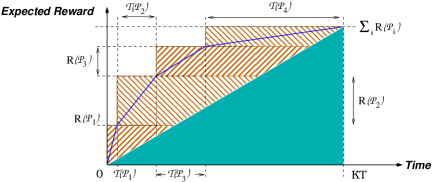
Figure 3: The accounting process of Lemma 3 explained pictorially.

Lemma 3.

The policy outlined in Figure 2 provides an expected reward of at least $\frac{1}{2}\sum_{i}R({\cal P}_{i})$.

Proof.

Let the number of plays of arm $i$ be $T_{i}$. We know $\mathbf{E}[T_{i}]=\mathcal{T}({\cal P}_{i})$ and $\sum_{i}\mathcal{T}({\cal P}_{i})\leq KT$. We start playing arm $i$ after $\sum_{j<i}T_{j}$ plays (if the sum is less than $T$); which means the remaining horizon for ${\cal P}_{i}$ is $T-\min\{T,\frac{1}{K}\sum_{j<i}T_{j}\}$. We apply the Truncation Theorem 2 with $\beta=1-\frac{1}{T}\min\{T,\frac{1}{K}\sum_{j<i}T_{j}\}$ and the expected reward of ${\cal P}_{i}$ continuing from that starting point onward is $\left(1-\frac{1}{T}\min\{T,\frac{1}{K}\sum_{j<i}T_{j}\}\right)R({\cal P}_{i})$. Note that this is a consequence of the independence of arm $i$ from $\sum_{j<i}T_{j}$. Thus the total expected reward $R$ is

$$R = \mathbf{E}\left[\sum_{i}\left(1-\frac{1}{T}\min\left\{T,\frac{1}{K}\sum_{j<i}T_{j}\right\}\right)R({\cal P}_{i})\right]\geq\mathbf{E}\left[\sum_{i}\left(1-\frac{1}{KT}\sum_{j<i}T_{j}\right)R({\cal P}_{i})\right]$$ (1)

$$= \sum_{i}\left(1-\frac{1}{KT}\sum_{j<i}\mathbf{E}[T_{j}]\right)R({\cal P}_{i})=\sum_{i}\left(1-\frac{\sum_{j<i}\mathcal{T}({\cal P}_{j})}{KT}\right)R({\cal P}_{i})$$

The bound in Equation 1 is best represented pictorially; for example consider Figure 3. Equation 1 indicates that $R$ is $\frac{1}{KT}$ fraction of the shaded area in Figure 3, which contains the triangle of area $\frac{1}{2}KT\sum_{i}R({\cal P}_{i})$. Therefore $R\geq\frac{1}{2}\sum_{j}R({\cal P}_{j})$ and the lemma follows. ∎

Theorem 4.

There exists a simple $2$-approximation for the finite horizon Bayesian MAB problem (with budgets and arbitrary priors) using an irrevocable scheduling policy. Such a policy can be found in polynomial time (solving a linear program).

Proof.

Given a collection of single arm policies $\{{\cal P}^{*}_{i}\}$ which correspond to the optimum solution of (LP1), we apply Lemma 3 with ${\cal P}_{i}={\cal P}^{*}_{i}$; since the collection $\{{\cal P}^{*}_{i}\}$ is feasible, namely, $\sum_{i}\mathcal{T}({\cal P}^{*}_{i})\leq KT$. Therefore the expected reward is at least $\frac{1}{2}\sum_{i}R({\cal P}^{*}_{i})\geq\frac{1}{2}\mbox{\sc LP1}$ and the theorem follows. ∎

Tight example of the analysis.

We show that the gap of the optimum policy and LP1 is a factor of $2-O(\frac{1}{n})$, even for unit length plays. Consider the following situation: We have two “types” of arms. The type I arm gives a reward $0$ with probability $a=1/n$ and $1$ otherwise. The type II arm always gives a reward $0$. We have $n$ independent arms. Each has an identical prior distribution of being type I with probability $p=1/n^{2}$ and type II otherwise. Set $T=n$.

Consider the symmetric LP solution that allocates one play to each arm; if it observed a $1$, it plays the arm for $n$ steps. The expected number of plays made is $n+O(1/n)$, and the expected reward is $n\times 1/n=1$. Therefore, $\mbox{\sc LP1}\geq 1-O(1/n)$.

Consider the optimum policy. We first observe that if the policy ever sees a reward $1$ then the optimum policy has found one of the type II arms, and the policy will continue to play this arm for the rest of the time horizon. At any point of time before the time horizon, since $T=n$, there is always at least one arm which has not been played yet. Suppose the policy plays an arm and observe the reward $0$, then the posterior probability of this arm being type II increased. So the optimum policy should not prefer this currently played arm over an unplayed arm. Thus the optimum policy would be to order the arms arbitrarily and make a single play on every new arm. If the outcome is $0$, the policy quits, otherwise the policy keeps playing the arm for the rest of the horizon. The reward of the optimum policy can thus be bounded by $\sum_{x=0}^{T-1}ap(1+(T-x-1)a)=pa^{2}T(T+1)/2+(1-a)/n=\frac{1}{2}+O(\frac{1}{n})$. Thus the gap is a factor of $2-O(\frac{1}{n})$.

3.4 Weak Coupling, Efficient Algorithms and Compact Representations

We outline how to solve (LP1) efficiently using a standard application of weak duality. Recall,

$$\mbox{\sc LP1}=\mbox{Max}_{\{P_{i}\in{\mathcal{C}}_{i}(T)\}}\left\{\sum_{i}R(P_{i})\ |\ \sum_{i}\mathcal{T}(P_{i})\leq KT\right\}$$

We take the Lagrangian of the coupling constraint to obtain:

$$\mbox{\sc LPLag}(\lambda)=\mbox{Max}_{\{P_{i}\in{\mathcal{C}}_{i}(T)\}}\left\{KT\lambda+\sum_{i}\left(R(P_{i})-\lambda\mathcal{T}(P_{i})\right)\right\}$$

Note now that there are no constraints connecting the arms, so that the optimal policy is obtained by solving LPLag$(\lambda)$ separately for each arm.

Definition 4.

Let $Q_{i}(\lambda)=\mbox{Max}_{P_{i}\in{\mathcal{C}}_{i}(T)}R(P_{i})-\lambda\mathcal{T}(P_{i})$ denote the optimal solution to $\mbox{\sc LPLag}(\lambda)$ restricted to arm $i$, so that $\mbox{\sc LPLag}(\lambda)=KT\lambda+\sum_{i}Q_{i}(\lambda)$. Let $\mathcal{L}_{i}(\lambda)$ denote the corresponding optimal policy for arm $i$. As a convention if $Q_{i}(\lambda)=0$ then we choose $\mathcal{L}_{i}(\lambda)$ to be the trivial policy which does nothing.

Lemma 5.

For any $\lambda\geq 0$ we have $\mbox{\sc LPLag}(\lambda)=\lambda KT+\sum_{i}Q_{i}(\lambda)\geq\mbox{\sc LP1}\geq OPT$.

The above Lemma is an easy consequence of weak duality. We now compute $Q_{i}(\lambda)$.

Lemma 6.

$Q_{i}(\lambda)$ and the corresponding single-arm policy $\mathcal{L}_{i}(\lambda)$ (completely specifying an optimum solution of LPLag$(\lambda)$) can be computed in time $O(\mbox{\sc\#Edges}{(}{\cal S}_{i}))$. For $\lambda\geq 0$, $R(\mathcal{L}_{i}(\lambda)),\mathcal{T}(\mathcal{L}_{i}(\lambda))$ and $Q_{i}(\lambda)$ are non-increasing as $\lambda$ increases.

Proof.

We use a straightforward bottom up dynamic program over the DAG represented by ${\cal S}_{i}(T)$ which is the statespace ${\cal S}_{i}$ restricted to a horizon $T$.

Let Gain$(u)$ to be the maximum of the objective of the single-arm policy conditioned on starting at $u\in{\cal S}_{i}(T)$. If $u$ has no children, then if we “play” at node $u$, then Gain$(u)=r_{u}-\lambda$ in this case. Stopping corresponds to Gain$(u)=0$. Therefore we set Gain$(u)=\max\{0,r_{u}-\lambda\}$ in this case. If $u$ had children, playing corresponds to a gain of $r_{u}-\lambda+\sum_{v}\mathbf{p}_{uv}\mbox{Gain}(v)$. Therefore:

$$\mbox{Gain}(u)=\mbox{Max}\left\{0,\ \ r_{u}-\lambda+\sum_{v}\mathbf{p}_{uv}\mbox{Gain}(v)\right\}$$

The policy $P_{u}$ constructed by the dynamic program rooted at $u\in S_{i}(T)$ satisfies the invariant $R(P_{u})=\mbox{Gain}(u)+\lambda\mathcal{T}(P_{u})$. This immediately implies Gain$(\rho_{i})=Q_{i}(\lambda)$. Note that we can ensure that Gain$(u)=0$ is obtained by the trivial policy at $u$ of doing nothing.

Moreover the decision to play at $\lambda^{\prime}$ also implies a decision to play at $\lambda<\lambda^{\prime}$. This trivially implies that $\mathcal{T}(\mathcal{L}_{i}(\lambda)),R(\mathcal{L}_{i}(\lambda))$ is non-increasing as $\lambda$ increases. Likewise, observe that for every $u\in{\cal S}_{i}(T)$, we have $\mbox{Gain}(u)$ is nonincreasing as $\lambda$ increases, and therefore $Q_{i}(\lambda)$ is nonincreasing. ∎

In terms of the variables of the original (LP1), $Q_{i}(\lambda)$ is defined as follows:

$$\begin{array}[]{rcll}\displaystyle Q_{i}(\lambda)&=&\displaystyle\mbox{Max}\sum_{i=1}^{n}\sum_{u\in{\cal S}_{i}(T)}(r_{u}-\lambda)z_{u}&\\ \sum_{v\in{\cal S}_{i}}z_{v}\mathbf{p}_{vu}&=&w_{u}&\forall i,u\in{\cal S}_{i}(T)\setminus\{\rho_{i}\}\\ z_{u}&\leq&w_{u}&\forall u\in{\cal S}_{i}(T),\forall i\\ z_{u},w_{u}&\in&[0,1]&\forall u\in{\cal S}_{i}(T),\forall i\\ \end{array}$$ (2)

The solution presented in Lemma 6 shows that the optimum policy $\mathcal{L}_{i}(\lambda)$ satisfies $z_{u}=0$ (no play, or Gain$(u)=0$) or $z_{u}=w_{u}$ (play orGain$(u)>0$); which are to expected using complementary slackness [14]. By a standard application of weak duality (see for instance [46]), a $(1+\epsilon)$ approximate solution to $(LP1)$ can be obtained by taking a convex combination of the solutions to LPLag$(\lambda)$ for two values $\lambda^{-}$ and $\lambda^{+}$; these can be computed by binary search. This yields the following.

Theorem 7.

In time $O((\sum_{i}\mbox{\sc\#Edges}{(}{\cal S}_{i}))\log(nT/\epsilon))$, we can compute quantities $a,\lambda^{-}$ and $\lambda^{+}$, where $|\lambda^{-}-\lambda^{+}|\leq\epsilon OPT/(KT)$ and a fraction $a\in[0,1)$ so that if ${\cal P}^{*}_{i}$ denotes the single-arm policy that executes $\mathcal{L}_{i}(\lambda^{-})$ with probability $a$ and $\mathcal{L}_{i}(\lambda^{+})$ with probability $(1-a)$, then these policies are feasible for (LP1) with objective at least $OPT/(1+\epsilon)$.

Proof.

Observe that for $\lambda=0$, if we satisfy the constraint $\sum_{i}\mathcal{T}(\mathcal{L}_{i}(\lambda))\leq KT$ then the theorem is immediately true based on Lemmas  3.1 and 6 (setting $\epsilon=0$). So in the remainder we assume that $\sum_{i}\mathcal{T}(\mathcal{L}_{i}(0))>KT$. Note that $OPT\leq\sum_{i}Q_{i}(0)$. Moreover, for all $i$, $OPT\geq Q_{i}(0)$ since the optimum can disregard all other arms. Let $M=\sum_{i}Q_{i}(0)$ and thus $M\leq nOPT$.

Now if we set $\lambda=2M$ then all $Q_{i}(\lambda)=0$ because the penalty of $\lambda$ to the root node is larger than the total reward of the policy. Thus all $\mathcal{L}_{i}(M)$ are the trivial null policy. In this case $\sum_{i}\mathcal{T}(\mathcal{L}_{i}(M))=0<KT$.

Therefore we can maintain the interval defined by the two numbers $\lambda^{-}<\lambda^{+}$ such that $\sum_{i}\mathcal{T}(\mathcal{L}_{i}(\lambda^{-}))>KT$ and $\sum_{i}\mathcal{T}(\mathcal{L}_{i}(\lambda^{+}))\leq KT$. Initially $\lambda^{-}=0$ and $\lambda^{+}=\infty$. We can now perform a binary search and maintain the properties till we have $\lambda^{+}-\lambda^{-}\leq\epsilon M/(2nKT)\leq\epsilon OPT/(2KT)$. Since $\sum_{i}\mathcal{T}(\mathcal{L}_{i}(\lambda^{-}))>KT\geq\sum_{i}\mathcal{T}(\mathcal{L}_{i}(\lambda^{+}))$ there exists an unique $a\in[0,1)$ such that

$$a\left(\mathcal{T}(\mathcal{L}_{i}(\lambda^{-}))\right)+(1-a)\left(\mathcal{T}(\mathcal{L}_{i}(\lambda^{+}))\right)=KT$$

Note that for such an $a$, we have $\sum_{i}\mathcal{T}({\cal P}_{i}^{*})=a\left(T(\mathcal{L}_{i}(\lambda^{-}))\right)+(1-a)\left(\mathcal{T}(\mathcal{L}_{i}(\lambda^{+}))\right)=KT$ thereby satisfying the main constraint in the compact representation of LP1. Observe that for $\lambda\in\{\lambda^{-},\lambda^{+}\}$,

$$\lambda KT+\sum_{i}\left\{R(\mathcal{L}_{i}(\lambda)-\lambda\mathcal{T}(\mathcal{L}_{i}(\lambda))\right\}\geq OPT$$ (3)

using the definition of $Q_{i}(\lambda),\mathcal{L}_{i}(\lambda)$ and Lemma 3.1. As a consequence, since $R({\cal P}_{i}^{*})=aR(\mathcal{L}_{i}(\lambda^{-})+(1-a)R(\mathcal{L}_{i}(\lambda^{+})$; we have:

$$OPT \leq a\left[\lambda^{-}KT+\sum_{i}\left\{R(\mathcal{L}_{i}(\lambda^{-})-\lambda^{-}\mathcal{T}(\mathcal{L}_{i}(\lambda^{-}))\right\}\right]+$$

$$\hskip 108.405pt(1-a)\left[\lambda^{+}KT+\sum_{i}\left\{R(\mathcal{L}_{i}(\lambda^{+})-\lambda^{+}\mathcal{T}(\mathcal{L}_{i}(\lambda^{+}))\right\}\right]$$

$$=(a\lambda^{-}+(1-a)\lambda^{+})KT+\sum_{i}R({\cal P}_{i}^{*})-\lambda^{-}\sum_{i}\mathcal{T}({\cal P}_{i}^{*})-(1-a)(\lambda^{+}-\lambda^{-})\sum_{i}\mathcal{T}(\mathcal{L}_{i}(\lambda^{+}))$$

and since $\sum_{i}\mathcal{T}({\cal P}^{*}_{i})=KT$ the last equation rewrites to

$$OPT\leq\sum_{i}R({\cal P}_{i}^{*})+(1-a)(\lambda^{+}-\lambda^{-})\left[KT-\sum_{i}\mathcal{T}(\mathcal{L}_{i}(\lambda^{+}))\right]$$

But that implies $OPT\leq\sum_{i}R({\cal P}_{i}^{*})+(1-a)(\lambda^{+}-\lambda^{-})KT\leq\sum_{i}R({\cal P}_{i}^{*})+\epsilon OPT/2$. Since for $x\in(0,1]$ we have $\frac{1}{1+x}\leq 1-x/2$ we have $OPT/(1+\epsilon)\leq\sum_{i}R({\cal P}_{i}^{*})$.

Observe that the initial size of the interval is $2M$ and the final size is at most $\epsilon M/(nKT)$. Therefore the number of binary searches is $\log\frac{nKT}{\epsilon}=O(\log(nT/\epsilon))$ since $k<n$. The theorem follows. ∎

Using Theorem 7, Lemma 3 and a rescaling of $\epsilon$ the following is immediate:

Corollary 8.

Given any $\epsilon\in(0,1]$, using $O((\sum_{i}\mbox{\sc\#Edges}{(}{\cal S}_{i}))\log(nT/\epsilon))$ time we can compute a $(2+\epsilon)$-approximation to the finite horizon Bayesian MAB using irrevocable policies.

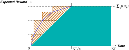
Figure 4: The accounting process of Corollary 9 explained pictorially.

Further applications of Theorem 7:

We prove a corollary which will be useful later;

Corollary 9.

If in time $O(\tau)$ we can compute an $c$-approximation to $\sum_{i}Q_{i}(\lambda,{\mathfrak{C}})$ where $Q_{i}(\lambda,{\mathfrak{C}})$ is $Q_{i}(\lambda)$ is defined by the maximizing system (2) with the additional constraint ${\mathfrak{C}}$ over single the arm policy; then we can compute a $(c+\epsilon)$-approximation for (LP1) for any $\epsilon\in(0,1]$, which satisfies $\sum_{i}\mathcal{T}({\cal P}_{i})=KT/c$ and the additional restriction over the same constraints ${\mathfrak{C}}$ over the single arm policies in time $O(\tau\log(nT/\epsilon))$. Further the scheduling policy in Figure 2 now provides a $\frac{2c(c+\epsilon)}{2c-1}$ approximation to $OPT({\mathfrak{C}})$ which is the optimum solution which obeys the constraint that $\sum_{i}\mathcal{T}({\cal P}_{i})\leq KT$ along with the single arm constraints ${\mathfrak{C}}$.

Proof.

A relaxation of $OPT({\mathfrak{C}})$ can be expressed as a mathematical program (${\mathfrak{C}}$ need not be linear constraints) where we have (LP1) with additional constraints ${\mathfrak{C}}$. However weak duality still holds and for any $\lambda\geq 0$,

$$\lambda KT+\sum_{i}Q_{i}(\lambda,{\mathfrak{C}})\geq OPT({\mathfrak{C}})$$ (4)

Now the proof of the corollary follows from replicating the proof of Theorem 7 with the following consequence of the approximation algorithm, instead of Equation (3),

$$\lambda KT+c\left(\sum_{i:\mathcal{L}_{i}(\lambda)\mbox{ obeys }{\mathfrak{C}}}\left\{R(\mathcal{L}_{i}(\lambda)-\lambda\mathcal{T}(\mathcal{L}_{i}(\lambda))\right\}\right)\geq OPT({\mathfrak{C}})$$ (5)

which follows from equation 4 and the $c$- approximation of $Q_{i}(\lambda,{\mathfrak{C}})$. Observe that now if we choose $\lambda^{-},\lambda^{+}$ such that $\sum_{i}\mathcal{T}(\mathcal{L}_{i}(\lambda^{-}))>KT/c\geq\sum_{i}\mathcal{T}(\mathcal{L}_{i}(\lambda^{+}))$ then we can ensure that $\sum_{i}\mathcal{T}({\cal P}^{*}_{i})=KT/c$. We still execute the policies as described in Figure 2, and the expected reward is at least (following the identical logic as in Lemma 3):

$$R^{\prime}\geq\sum_{i}\left(1-\frac{\sum_{j<i}\mathcal{T}({\cal P}_{j})}{KT}\right)R({\cal P}_{i})$$

Pictorially, $R^{\prime}$ is at least $\frac{1}{KT}$ times the area of the shaded triangle and the rectangle as shown in Figure 4, which amounts to $(1-\frac{1}{2c})\sum_{i}R({\cal P}_{i})$. Observe that $c=1$ corresponds to the statement of Lemma 3. The overall approximation is therefore $\frac{2c(c+\epsilon)}{2c-1}$ which proves the theorem. ∎

3.5 Comparison to Gittins Index

The most widely used policy for the discounted version of the multi-armed bandit problem is the Gittins index policy [33]. Recall the single-arm policies constructed in Section 3.4. For arm $i$, consider the policy $\mathcal{L}_{i}(\lambda)$ corresponding to the value $Q_{i}(\lambda)$. We can account for the reward of this policy as follows. Suppose any policy is given fixed reward $\lambda$ per play (so that if the expected number of plays is $\mathcal{T}(P)$, the policy earns $\lambda\mathcal{T}(P)$). Then, the value $Q_{i}(\lambda)$ is the optimal excess reward a policy can earn given these average values, since this is precisely $\max_{P\in{\mathcal{C}}_{i}}(R(P)-\lambda\mathcal{T}(P))$. To solve our relaxation (LP1), we find $\lambda$ so that the total expected number of plays made by the single-arm policies for different $i$ sums to $T$. The definition of $Q_{i}(\lambda)$ can be generalized to an equivalent definition $Q_{i}(\lambda,u)$ for policies whose start state is $u\in{\cal S}_{i}(T)$ (instead of being the root $\rho_{i}$). The Gittins index for $u\in{\cal S}_{i}(T)$ can be defined as:

$$\mbox{Gittins Index}=\Pi_{i}(u)=\max\{\lambda\ |\ Q_{i}(\lambda,u)>0\}$$

In other words, the Gittins index for state $u$ is the maximum value of $R(P)/\mathcal{T}(P)$ over policies restricted to starting at state $u$ (and making at least one play), i.e., the maximum amortized per-step long term reward obtainable by playing at $u$. The Gittins index policy works as follows: At any time step, play the arm $i$ whose current state $u$ has largest index $\Pi_{i}(u)$. For the discounted reward version of the problem, such an index policy yields the optimal solution. This is not true for the finite horizon version, and the other variants we consider below. Nevertheless, the starting point for our algorithms is the solution to (LP1), and as shown above, this has computational complexity similar to the computation of the Gittins index.

In contrast to the Gittins index, our policies are based on computing (as in Theorem 7) one global penalty $\lambda^{*}$ across all arms by solving (LP1); consider the case $\lambda^{+}\approx\lambda^{*}\approx\lambda^{-}$ in Theorem 7. For this penalty, for each arm $i$ and state $u\in{\cal S}_{i}(T)$, the policy $\mathcal{L}_{i}(\lambda^{*})$ makes a decision on whether to play or not play. We execute these decisions, and impose a fixed priority over arms to break ties in case multiple arms decide to play.

4 Traversal Dependent Bayesian MAB Problems

In this section we consider how the constraints on a traversal of different bandit arms can affect the approximation algorithm. A concrete example of such traversal related constraint is the Bayesian MAB Problem with Switching Costs where there is a cost of switching between arms. Denote the cost of switching from arm $i$ to arm $j$ as $\ell_{ij}\in\mathcal{Z}^{+}$. The system starts at an arm $i_{0}$. The goal is to maximize the expected reward subject to rigid constraints that (i) the total number of plays is at most $T$ and (ii) the total switching cost is at most $L$ on all decision paths. This problem has received significant attention, see the discussion in Section 1 and in [12] - however efficient solutions with provable bounds in the Bayesian setting has been elusive.

A classic example of such a switching cost problem can be when the costs $\ell_{ij}$ define a distance metric, which is natural in most navigational settings and was considered earlier in [40]. Here we will provide a $X$ approximation for that problem improving the $12$-approximation provided in [40].

However a strong motivation of this section is to continue developing general techniques for Bayesian MAB problems and therefore we take a slightly indirect route. We first consider a different problem: Finite Horizon Bayesian MAB using Arbitrary Order Irrevocable Policies. In this problem, once we have decided upon the set of arms to play then an adversary provides us with a specific order such that if we start playing an arm $i$ then we cannot visit/revisit any arm before arm $i$ in that said order. We will provide an efficient (again near linear time in the input sparsity) $Y$-approximation for this problem. Since switching costs are often used to model economic interactions in the Bandit setting, as in [12, 32, 47, 53], the adversarially ordered traversal problem is an interesting subproblem in its own right. In addition, there are two key benefits of this approach.

• First, the analysis technique for arbitrary (or adversarial) order will disentangle the decisions between the constraint associated with the traversal and the constraint associated with the finite horizon. Note that all these traversal problems encode a natural combinatorial optimization problem and are often MAX SNP Hard — and this disentanglement and isolation of the combinatorial difficulty produces natural policies.

• Second, because we use irrevocable policies, the switching cost is only relevant for the algorithm for the first transition from $i$ to $j$. The proof presented herein will remain exactly the same if the second transition of $i$ to $j$ costs more or less than the first transition, as long as the costs are positive!

Roadmap: We first discuss the Arbitrary Order Irrevocable Policy problem in Section 4.1. We then show in Section 4.2 how the analysis applies to the Bayesian MAB problem with Metric Switching costs; the analysis will extend beyond the metric assumption as long as a certain traversal type problem (Orienteering Problem) can be approximated to small factors in polynomial time.

4.1 Arbitrary Order Irrevocable Policies for the Bayesian MAB Problem

The set up of this problem is similar to the Finite Horizon MAB problem using irrevocable policies discussed in Section 3. The only difference is that we cannot use the ordering of $R({\cal P}_{i})/T(P_{i})$ as described in the scheduling policy in Figure 2 – instead we will have to use an arbitrary order after the arms and the corresponding policies ${\cal P}_{i}$ have been chosen, that is, the Step 2 is not performed. Note that the bound of LP1 remains a valid upper bound of this problem – but Lemma 3 does not apply explicitly and Theorem 7 is not useful implicitly. In what follows, we prove Theorem 10 which replaces them. The notation used will be the same as in Section 3.

The Final Adversarial Order Irrevocable Policy 1. Solve (LP1) to obtain a collection of single-arm policies ${\cal P}_{i}$. 2. For each $i$, create policy ${\cal P}^{\prime}_{i}$ which chooses to plays ${\cal P}_{i}$ with probability $\alpha\in(0,1]$ and with probability $(1-\alpha)$ is the null policy. 3. An adversary orders the arms determining the order in they have to be played. 4. Start with the first $K$ policies in the order specified in Step 3. These policies are inspected; the remaining policies are uninspected. (a) If the decision in ${\cal P}^{\prime}_{i}$ is to quit, then move to the first uninspected arm in the order (say ${\cal P}^{\prime}_{j}$) and start executing ${\cal P}^{\prime}_{j}$. This is similar to scheduling $K$ parallel machines. (b) If the horizon $T$ is reached, the overall policy stops execution. Note $KT\geq\sum_{i}\mathcal{T}({\cal P}^{\prime}_{i})$.

Figure 5: Scheduling where an adversary to decides the traversal order

Theorem 10.

The Finite Horizon Bayesian MAB Problem using arbitrary order irrevocable policies has a $4$ approximation that can be found in polynomial time and a $(4+\epsilon)$-approximation in $O((\sum_{i}\mbox{\sc\#Edges}{(}{\cal S}_{i}))\log(nT/\epsilon))$ time using the scheduling policy in Figure 5.

Proof.

Using the exact same initial arguments as in Lemma 3 we arrive at the inequality 1 which states that the expected reward $R^{\prime}$ in this case satisfies:

$$R^{\prime}\geq\sum_{i}\left(1-\frac{\sum_{j<i}\mathcal{T}({\cal P}^{\prime}_{j})}{KT}\right)R({\cal P}^{\prime}_{i})\geq\left(1-\frac{\sum_{j}\mathcal{T}({\cal P}^{\prime}_{j})}{KT}\right)\sum_{i}R({\cal P}^{\prime}_{i})$$

Now observe that $R({\cal P}^{\prime}_{i})=\alpha R({\cal P}_{i})$ and $\mathcal{T}({\cal P}^{\prime}_{i})=\alpha\mathcal{T}({\cal P}^{\prime}_{i})$ and therefore $R^{\prime}\geq\alpha(1-\alpha)\sum_{i}R({\cal P}_{i})$. Using an exact solution or Theorem 7, and setting $\alpha=\frac{1}{2}$ the statement in this theorem follows. ∎

However note that there is a slack in the above analysis because in Step 1 in the policy in Figure 5, we could have found weakly coupled policies that take a combined horizon of $2KT$. Balancing this slack will provide us with an alternate optimization which is useful if we cannot compute $Q_{i}(\lambda)$ or (LP1) in a near optimally fashion. One such example is the Finite Horizon Bayesian MAB Problem with Metric Switching Costs, which we discuss next.

4.2 Bayesian MAB Problem with Metric Switching Costs

For simplicity we also assume $K=1$ in this section, that is, the system is allowed to play only one arm at a time and observe only the outcome of that played arm. We discuss the $K>1$ at the end of the subsection. The system starts at an arm $i_{0}$. A policy, given the outcomes of the actions so far (which decides the current states of all the arms), makes one of the following decisions (i) play the arm it is currently on; (ii) play a different arm (paying the distance cost to switch to that arm); or (iii) stop. Just as before, a policy obtains reward $r_{u}$ if it plays arm $i$ in state $u\in{\cal S}_{i}$. Any policy is also subject to rigid constraints that the total number of plays is at most $T$ and the total distance cost is at most $L$ on all decision paths. To begin with, we delete all arms $j$ such that $\ell_{i_{0}j}>L$. No feasible policy can reach such an arm without exceeding the distance cost budget. Let $OPT$ denote both the optimal solution as well as its expected reward.

4.2.1 A (Strongly Coupled) Relaxation and its Lagrangian

We describe a sequence of relaxations to the optimal policy, culminating with a weakly coupled relaxation. A priori, it is not clear how to construct such a relaxation, since the switching cost constraint couples the arms together in an intricate fashion. We achieve weak coupling via the Lagrangian of a natural LP relaxation, which we show can be solved as a combinatorial problem called orienteering over single-arm policies.

Definition 5.

Let ${\mathcal{C}}(L,T)$ denote the set of policies on all the remaining arms, over a time horizon $T$, that can perform one of two actions: (1) Play current arm; or (2) Switch to different arm. Such policies have no constraints on the total number of plays, but are required to have distance cost $L$ on all decision paths. Observe that if the constraint corresponding to the distance constraint is removed then $P\in{\mathcal{C}}(L,T)$ will decompose to $\{P_{i}\in{\mathcal{C}}_{i}(T)\}$, that is, the single arm policies $P_{i}$ (which are the projections of $P$) have at most a horizon of $T$ (See Definition 1 for the definition of ${\mathcal{C}}_{i}(T)$).

Given a policy $P\in{\mathcal{C}}(L,T)$ define the following quantities in expectation over the decision paths: Let $R(P)$ be the expected reward obtained by the policy and let $\mathcal{T}(P)$ denote the expected number of plays made. Note that any policy $P\in{\mathcal{C}}(L,T)$ needs to have distance cost at most $L$ on all decision paths. Consider the following optimization problem, which is still strongly coupled since ${\mathcal{C}}(L,T)$ is the space of policies over all the arms, and not the space of single-arm policies:

$$(M1):\qquad\mbox{Max}_{P\in{\mathcal{C}}(L,T)}\left\{R(P)\left|\ \mathcal{T}(P)\leq T\right.\right\}$$

Proposition 1.

$OPT$ is feasible for $(M1)$.

Proof.

We have $\mathcal{T}(OPT)\leq T$; since $OPT\in{\mathcal{C}}(L,T)$, this shows it is feasible for $(M1)$. ∎

Let the optimum solution of $(M1)$ be $OPT^{\prime}$ and the corresponding policy be $P^{*}$ such that $R(P^{*})=OPT^{\prime}\geq OPT$. Note that $P^{*}$ need not be feasible for the original problem, since it enforces the time horizon $T$ only in expectation over the decision paths. We now consider the Lagrangian of the above for $\lambda>0$, and define the problem $M2(\lambda)$:

Definition 6.

Let $V(\lambda)=\mbox{\rm Max}_{P\in{\mathcal{C}}(L,T)}\left(R(P)-\lambda\mathcal{T}(P)\right)$. Let $M2(\lambda)$ be $\mbox{\rm Max}_{P\in{\mathcal{C}}(L,T)}f_{\lambda}(P)$. For a policy $P\in{\mathcal{C}}(T)$ let $f_{\lambda}(P)=\lambda T+R(P)-\lambda\mathcal{T}(P)$. Then,

$$M2(\lambda):\qquad\mbox{\rm Max}_{P\in{\mathcal{C}}(L,T)}\ \ f_{\lambda}(P)=\lambda T+\mbox{\rm Max}_{P\in{\mathcal{C}}(L,T)}\left(R(P)-\lambda\mathcal{T}(P)\right)=\lambda T+V(\lambda)$$

We first relate $OPT$ to the optimal value $\lambda T+V(\lambda)$ of the problem $M2(\lambda)$.

Lemma 11.

For any $\lambda\geq 0$, we have $M2(\lambda)=\lambda T+V(\lambda)\geq OPT$.

Proof.

This is simply weak duality: For the optimal policy $P^{*}$ to $(M1)$, we have $\mathcal{T}(P^{*})\leq T$. Since this policy is feasible for $M2(\lambda)$ for any $\lambda\geq 0$, the claim follows. ∎

In the Lagrangian formulation, if arm $i$ is played in state $u\in{\cal S}_{i}$, the expected reward obtained is $r_{u}-\lambda$. We re-iterate that the only constraint on the set of policies ${\mathcal{C}}$ is that the distance cost is at most $L$ on all decision paths.

4.2.2 Structure of $M2(\lambda)$

The critical insight, which explicitly uses the fact that in the MAB the state of an inactive arm does not change and which allows weak coupling, is the following:

Lemma 12.

For any $\lambda\geq 0$, given any $P\in{\mathcal{C}}$, there exists a $P^{\prime}\in{\mathcal{C}}$ that never revisits an arm that it has already played and switched out of, such that $f_{\lambda}(P^{\prime})\geq f_{\lambda}(P)$.

Proof.

We will use the fact that ${\cal S}_{i}$ is finite in our proof. Suppose $P\in{\mathcal{C}}$ revisits an arm. Consider the last point in time, denote this $\alpha$, where the policy is at some arm $i$, makes a decision to switch to arm $j$ and at some subsequent point in time on some decision path, revisits arm $i$. Note that after time $\alpha$, the subsequent decision policy $P_{\alpha}$ satisfies the condition that no arm is revisited. Therefore, all plays of arm $j$ are contiguous in time within the policy $P_{\alpha}$. Let $\tilde{P}$ denote the decision policy subsequent to exiting arm $j$; this policy can be different depending on the outcomes of the plays for arm $j$. However, since any such $\tilde{P}$ never revisits arm $j$, we can simply choose that policy $\tilde{P^{*}}$ with maximum $f_{\lambda}(\tilde{P})$ and execute it regardless of the outcomes of the plays of arm $j$. This yields a new policy $P^{\prime}$ so that $f_{\lambda}(P^{\prime})\geq f_{\lambda}(P)$, and furthermore, the distance cost of $P^{\prime}$ is at most $L$ in all decision paths, so that $P^{\prime}$ is feasible. By the repeated application of this procedure, the decision policy $P_{\alpha}$ can be changed to the following form without decreasing $f_{\lambda}(P)$: The new policy makes an adaptive set of plays arm $j$; regardless of the outcomes of these plays, the policy switches to the same next arm $k$, again makes an adaptive set of plays; transitions to the same next arm $l$ regardless of the outcome of the plays, and so on, without ever revisiting an arm. We will refer to such a policy as a “path” over arms.

Recall that the overall decision policy is at arm $i$ just before time $\alpha$. Suppose this arm is revisited in the path $P_{\alpha}$, so that an adaptive set of plays is made for this arm. We modify the policy to make these plays at time $\alpha$, and then switch to arm $j$ regardless of the outcome of these plays. Suppose the original path $P_{\alpha}$ visited arm $i$ from arm $k$ and subsequently switched from $i$ to $l$ regardless of the outcomes of the plays of $i$, the new policy switches from arm $k$ directly to arm $l$. Since the states of arms that are not played never changes, this movement preserves the states of all the arms, and the moved plays for arm $i$ are stochastically identical to the original plays. Further, the distance cost of the new policy is only smaller, since the cost of switching into and out of arm $i$ is removed. This eliminates $\alpha$ as the last time when the policy is at some arm which is subsequently revisited. By repeated application of the above procedure, the lemma follows. ∎

Note that the above is not true for policies restricted to be feasible for $(M1)$. This is because the step where we use policy $\tilde{P}$ regardless of the outcome of the plays for arm $j$ need not preserve the constraint $\mathcal{T}(P)\leq T$, since this depends on the number of plays made for arm $j$. The Lagrangian $M2(\lambda)$ makes the overall objective additive in the (new) objective values for each arm, with the only constraint being that the distance cost is preserved. Since this cost is preserved in each decision branch, it is preserved by using the best policy $\tilde{P}$ regardless of the outcome of the plays for $j$.

4.2.3 Orienteering and the Final Algorithm

We now show that the optimal solution to M2$(\lambda)$ is a collection of single-arm policies connected via a combinatorial optimization problem termed orienteering.

Definition 7.

In the orienteering problem [17, 13, 22], we are given a metric space $G(V,E)$, where each node $v\in V$ has a reward $o_{v}$. There is a start node $s\in V$, and a distance bound $L$. The goal is to find that tour $P$ starting at $s$, such that $\sum_{v\in P}o_{v}$ is maximized, subject to the length of the tour being at most $L$. Observe that for any given any $\varepsilon\in(0,1]$ we can discretize $\{o_{v}|o_{v}>0\}$ such that within a $(1+\varepsilon)$ approximation we can assume that $o_{v}$ are integers which are at most $O(n/\varepsilon)$.

An immediate consequence of Lemma 12 is the following:

Corollary 13.

Define a graph $G(V,E)$, where node $i\in V$ corresponds to arm $i$. The distance between nodes $i$ and $j$ is $\ell_{ij}$, and the reward of node $i$ is $o_{i}=Q_{i}(\lambda)$. The optimum solution $V(\lambda)$ of $M2(\lambda)$ is the optimal solution to the orienteering problem on $G$ starting at node $i_{0}$ and respecting rigid distance budget $L$.

Proof.

Consider any $n$-arm policy $P\in{\mathcal{C}}$. By Lemma 12, the decision tree of the policy can be morphed into a sequence of “super-nodes”, one for playing each arm, such that the decision about which arm to play next is independent of the outcomes for the current arm. The policy maximizing $f_{\lambda}(P)$ will therefore choose the best policy in ${\mathcal{C}}_{i}$ for each single arm as the “super-node”(obtaining objective value precisely $Q_{i}(\lambda)$), and visit these subject to the constraint that the distance cost is at most $L$. This is precisely the orienteering problem on the graph defined above. ∎

Theorem 14.

For any $\epsilon\in(0,1]$ the orienteering problem has a $(2+\epsilon)$-approximation that can be found in polynomial time [22]. The authors of [17] showed that any $c$-approximation for $K=1$ case (where we choose a single tour) extends to an $(c+1)$-approximation for the $K>1$ case where we choose $K$ tours.

We are now ready to present the main theorem for this application,

Theorem 15.

For the finite-horizon multi-armed bandit problem with metric switching costs, for $K=1$ play at a time step there exists a polynomial time computable ordering of the arms and a policy for each arm, such that a solution which plays the arms using those fixed policies, in that fixed order without revisiting any arm, has reward at least $1/(4+\varepsilon)$ times that of the best adaptive policy, for any $\varepsilon\in(0,1]$. For $K>1$ the the reward is at least $1/(4.5+\varepsilon)$.

Proof.

We will use Corollary 9 and use the scheduling policy in Figure 5 setting $\alpha=1$. Note that using Lemma 13, the constraints ${\mathfrak{C}}$ are null! The traversal constraint does not imply any constraints on the internals of a single arm policy. However $OPT({\mathfrak{C}})$ still has a rigid constraint of a traversal cost of at most $L$.

Based on the $c(K)$ approximation algorithm and Corollary 9 we have a collection of policies $\{{\cal P}_{i}\}$ such that (i) $\sum_{i}\mathcal{T}({\cal P}_{i})=KT/c(K)$ and (ii) $c(K)\sum_{i}R({\cal P}_{i})\geq OPT(K)$ where $c(K)$ is the approximation factor determined by Theorem 14 and $OPT(K)$ is the corresponding optimum solution (again under the rigid traversal cost $L$). Now observe that the reward $R^{\prime\prime}$ we obtain satisfies:

$$R^{\prime\prime}\geq\left(1-\frac{\sum_{j}\mathcal{T}({\cal P}^{\prime}_{j})}{KT}\right)\sum_{i}R({\cal P}^{\prime}_{i})\geq\left(1-\frac{1}{c(K)}\right)\frac{1}{c(K)}OPT(K)$$

The theorem follows using $c(1)=2+\epsilon$ and $c(K)=3+\epsilon$ where $\epsilon=\varepsilon/12$. Note that if $c(K)\leq 2$ then we should have used $\alpha=\min\{1,c(K)/2\}$. ∎

Remark:

Note that the above technique is powerful enough to approximate any switching cost problem as long as the basic combinatorial problem is approximable. We note that there exists approximations for asymmetric distances (directed graphs with triangle inequality) and other traversal problems in [17]. Modifications to Theorem 15 will provide a solution for all such problems.

5 Multi-armed Bandits with Delayed Feedback

In this variant of the MAB problem, if an arm $i$ is played, the feedback about the reward outcome is available after $\delta_{i}$ time steps. Once again the budgets of the arms is encoded in the respective state spaces. In this section we assume that there are no switching or traversal dependent costs. Given the algorithms and analysis we propose for handling delayed feedback, such additional constraints can be handled using the ideas of the preceding sections.

From an analysis standpoint, the idea of truncation is not (immediately) useful. This is because a policy can (and should) be “back-loaded” in the sense that if we consider a single arm, most of the plays are made towards the end of the horizon (possibly because the policy is confident that the reward of this arm is large and well separated from the alternatives). Therefore truncating the horizon (by any factor) may cause these good plays to be eliminated and as a consequence we would not have any guarantee on the expected reward. In what follows we will introduce two techniques that avoid the problem mentioned:

1. A Delay Free Simulation; where at some point of time in the policy, the delays become irrelevant.

2. A Block Compaction Strategy; where the plays of a policy are moved earlier in time.

Of course, both of these ideas lose optimality, but interestingly that loss of optimality can be bounded. These two techniques are similar, they both increase the number of plays, and yet are useful in very different regimes. The delay free simulation idea, by itself gives us a $(2(1+\epsilon)+32(y+y^{2}))$-approximation for any $\epsilon\in(0,1]$ where $y=\max_{i}\delta_{i}/\sqrt{T}$. This implies that when the delay is small, the result is very close to the finite horizon MAB result discussed in Section 3 except that we are not using irrevocable policies. For $\max_{i}\delta_{i}\leq\sqrt{T}/50$ this approximation ratio is less than $3$. However this idea ceases to be less useful by itself as $\max_{i}\delta_{i}$ increases. The block compaction strategy (in conjunction with the delay free simulation) allows an $O(1)$ approximation even when $\delta_{i}$ are large as long as $21(2\delta_{i}+1)(1+\log\delta_{i})\leq T$ for all $i$.

Note that it is not immediate how to construct good policies for $\max_{i}\delta_{i}$ is a non-trivial constant (say $100$) or even the larger regime without losing factors proportional to $\max_{i}\delta_{i}$. Thus it is doubly interesting that these two regimes naturally emerge from the analysis of approximation factors – these two regimes expose two different scheduling ideas. We come a full circle from the discussion in Ehrenfeld [27], where the explicit connections between stopping rules for delayed feedback in the two bandit setting and scheduling policies were considered.

The Overall Plan and Roadmap:

We will bound the optimum using single arm policies. In both regimes of $\max_{i}\delta_{i}$, instead of solving the relaxations, we first show that there exists a subclass of policies which (i) have much more structure, (ii) preserve the approximation bound with respect to the globally optimum policies and (iii) are easy to find. We first present the basic notation and definitions in Section 5.1. We then discuss the regime where $\max_{i}\delta_{i}\leq\sqrt{T}/10$ in Section 5.2 and prove the relevant approximation bound in Lemma 20, under the assumption that we can find the suitable policies. In the interest of the presentation we do not immediately show how to compute the policies but we discuss the regime where $\delta_{i}$ are larger (but $21(2\delta_{i}+1)(1+\log\delta_{i})\leq T$ for all $i$) next in Section 5.3 and prove the approximation bound in Lemma 22, under the same assumption that we can find the suitable policies. Finally we show how to compute the policies in polynomial time, using a linear program in Section 5.4. That linear program can also be solved to a $(1+\epsilon)$-approximation efficiently using ideas in the previous sections. As a consequence,

Theorem 16.

We can approximate the finite horizon Bayesian MAB problem with delayed feedback to a $2(1+\epsilon)+32(y+y^{2})$ approximation where $y=\max_{i}\delta_{i}/\sqrt{T}$ for any $\epsilon>0$ in polynomial time. If the delays are small constants or $o(\sqrt{T})$ then this result implies a $(2+o(1))$-approximation which seamlessly extends Theorem 4. For $\max_{i}\delta_{i}\leq T/(48\log T)$ we provide a $O(1)$ approximation in polynomial time.

5.1 Weakly Coupled Relaxation and Block Structured Policies

Single arm policies:

In the case of delayed feedback, describing a single-arm policy is more complicated. This policy is now a (randomized) mapping from the current state of the arm to one of the following actions: (i) make a play; (ii) wait some number of steps (less or equal to $T$), so that when the result of a previous play is known, the policy changes state; (iii) wait a few steps and make a play (without extra information); or (iv) quit.

Definition 8.

Let ${\mathcal{C}}_{i}(T,\delta_{i})$ be the set of all single-arm policies over a horizon of $T$ steps.

As in Section 3, we will use the LP system (LPDelay) to bound of the reward of the best collection of single-arm policies - the goal will be to find one policy per arm so that the total expected number of plays is at most $T$ and the expected reward is maximized. This is expressed by the following relaxation:

$$\mbox{\sc LPDelay}=\mbox{Max}_{\{P_{i}\in{\mathcal{C}}_{i}(T,\delta_{i})\}}\left\{\sum_{i}R(P_{i})\ |\ \sum_{i}\mathcal{T}(P_{i})\leq T\right\}$$

The state of the system is now captured by not only the current posterior $u\in{\cal S}_{i}$, but also the plays with outstanding feedback and the remaining time horizon. Note that the state encodes plays with outstanding feedback, and this has size $2^{\delta_{i}}$, which is exponential in the input. Therefore, it is not even clear how to solve (LPDelay) in polynomial time, and we use (LPDelay) as an initial formulation for the purposes of an upper bound.

Definition 9.

A single-arm policy is said to be Block Structured if the policy executes in phases of size $(2\delta_{i}+1)$. At the start of each phase (or block), the policy makes at most $\delta_{i}+1$ consecutive plays. The policy then waits for the rest of the block in order to obtain feedback on these plays, and then moves to the next block. A block is defined to be full if exactly $\delta_{i}+1$ plays are made in it. Let the class of Block Structured policies for arm $i$ over a horizon $T$ be ${\mathcal{C}}^{b}_{i}(T,\delta_{i})$.

We first show that all single-arm policies can be replaced with block structured policies while violating the time horizon by a constant factor. The idea behind this proof is simple – we simply insert delays of length $\delta_{i}$ after every chunk of plays of length $\delta_{i}$.

Lemma 17.

Any policy ${\cal P}\in{\mathcal{C}}_{i}(T,\delta_{i})$ can be converted it to a Block Structured policy ${\cal P}^{\prime}\in{\mathcal{C}}^{b}_{i}(2T,\delta_{i})$ such that $R({\cal P})\leq R({\cal P}^{\prime})$ and $\mathcal{T}({\cal P}^{\prime})\leq\mathcal{T}({\cal P})$ (note that the horizon increases).

Proof.

We can assume that the policy makes a play at the very first time step, because we can eliminate any wait without any change of behavior of the policy.

Consider the actions of ${\cal P}$ for the first $\delta_{i}+1$ steps, the result of any play in these steps is not known before all these plays are made. An equivalent policy ${\cal P}^{\prime}$ simulates ${\cal P}$ for the first $\delta_{i}+1$ steps, and then waits for $\delta_{i}$ steps, for a total of $2\delta_{i}+1$ steps. This ensures that ${\cal P}^{\prime}$ knows the outcome of the plays before the next block begins.

Now consider the steps from $\delta_{i}+2$ to $2\delta_{i}+3$ of ${\cal P}$. As ${\cal P}$ is executed, it makes some plays possibly in an adaptive fashion based on the outcome of the plays in the previous $\delta_{i}+1$ steps, but not on the current $\delta_{i}+1$ steps. ${\cal P}^{\prime}$ however knows the outcome of the previous plays, and can simulate ${\cal P}$ for these $\delta_{i}+1$ steps and then wait for $\delta_{i}$ steps again. It is immediate to observe that ${\cal P}^{\prime}$ can simulate ${\cal P}$ at the cost of increasing the horizon by a factor of $\frac{2\delta_{i}+1}{\delta_{i}+1}<2$. Observe that in each block of $2\delta_{i}+1$, ${\cal P}^{\prime}$ can make all the plays consecutively at the start of the block without any change in behavior. The budgets are also respected in this process. This proves the lemma. ∎

We now show how to find a set of block structured policies $\{{\cal P}_{i}\}$ such that each has horizon at most $2T$ and together satisfy the following properties $\sum_{i}R({\cal P}_{i})\geq\mbox{\sc LPDelay}$ and $\sum_{i}\mathcal{T}({\cal P}_{i})\leq KT$. Observe that by Lemma 17, such policies exist.

Lemma 18.

We find a collection of policies $\{{\cal P}_{i}|{\cal P}_{i}\in{\mathcal{C}}^{b}_{i}(2T,\delta_{i})\}$ such that $\sum_{i}R({\cal P}_{i})\geq\mbox{\sc LPDelay}/(1+\epsilon)$ and $\sum_{i}\mathcal{T}({\cal P}_{i})\leq KT$ for any $\epsilon\in(0,1]$ in time polynomial in $\sum_{i}{\cal S}_{i},T$ (using a linear program or a fast approximate solution for such).

We relegate the proof of Lemma 18 to Section 5.4 and continue with the algorithmic development.

5.2 Delay Free Simulations and Small Delays

In this section we discuss the case when the delays are small in comparison to the horizon, i.e., $\max_{i}\delta_{i}\leq\sqrt{T}/50$. We next introduce the delay free simulation idea. Let $r=\sqrt{T}/(2\max_{i}\delta_{i})$ and $\gamma=4r(\max_{i}\delta_{i})^{2}/T$. The choice of these parameters will become clear shortly.

Definition 10.

Define a policy ${\cal P}_{i}$ to be in a delay-free mode at time $t$ if at time $t$ the policy ${\cal P}_{i}$ makes a play, but uses the outcome of a play made at time $t-\delta_{i}$ (or earlier). The outcome of the current play is available at time $t+\delta_{i}$ and can be used subsequently.

Observe that the truncation idea of Theorem 2 applies to a policy once it is in a delay free mode.

Definition 11.

Define a policy ${\cal P}_{i}$ to be a $(\gamma T,T)$-horizon policy if the policy is block structured on all decision paths till a horizon of $\gamma T$ and subsequently makes at most $T$ plays in a delay free mode. A pictorial depiction of a $(\gamma T,T)$-horizon policy is shown if Figure 6.

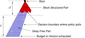
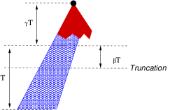
Figure 6: Part (a) shows an example $(\gamma T,T)$-horizon policy; the part marked in solid red is block structured and the patterned blue part is in delay free mode. Part (b) shows the same policy when it is truncated at horizon $(\gamma+\beta)T$ where $\beta\in(0,1)$. In the accounting step we ensure that to receive any reward from the policy, the entire block structured part has to be played, i.e., $\beta>0$. Subsequently we can argue that the reward of the policy in (b) is at least $\beta$ times that of the policy in (a) – note that the argument is made on a path-by-path basis and we do not need a strong characterization of the decision boundary.

Lemma 19.

Given any block structured policy ${\cal P}\in{\mathcal{C}}^{b}_{i}(2T,\delta_{i})$ we can construct a $(\gamma T,T)$-horizon policy ${\cal P}^{\prime}$ such that $R({\cal P})\leq R({\cal P}^{\prime})$ and $\mathcal{T}({\cal P}^{\prime})\leq(1+\frac{1}{r})\mathcal{T}({\cal P})$.

Proof.

Consider the first time the policy ${\cal P}$ makes $r\delta_{i}$ plays on some decision path. Define a new policy ${\cal P}^{\prime}$ as follows: It is identical to ${\cal P}$ till the end of the block that contains the $r\delta_{i}$-th play and then it makes $\delta_{i}$ additional plays. Let these plays be $z(1),z(2),\ldots,z(\delta_{i})$. Note that ${\cal P}$ was not making any plays and waiting for the end of the block. After this point, consider the $t$-th play made by ${\cal P}$ where $t\leq\delta_{i}$ – the policy ${\cal P}^{\prime}$ makes the play but simply uses the outcome of $z(t)$ which is known by now. The outcome of the $t$-th play is not known (or used) and would only be used for the $t+\delta_{i}$-th play. Note that since the outcome of two plays are from the same underlying distribution we can couple the outcomes to be identical as well. If ${\cal P}$ decides to stop execution, then ${\cal P}^{\prime}$ stops execution as well. Clearly, ${\cal P}^{\prime}$ makes $\delta_{i}$ additional plays than ${{\cal P}}$ on any decision path. Since ${\cal P}$ made at least $r\delta_{i}$ plays by then, this shows that $\mathcal{T}({\cal P}^{\prime})\leq(1+\frac{1}{r})\mathcal{T}({\cal P})$. Since the execution of ${\cal P}^{\prime}$ is coupled play-by-play with the execution of ${\cal P}$, it is clear that $R({\cal P})\leq R({\cal P}^{\prime})$.

Observe that once ${\cal P}^{\prime}$ has switched to this “delay free mode” then ${\cal P}^{\prime}$ can now simply ignore the blocks, but would make at most $T$ plays. This switch to a delay free mode must occur within the first $r\delta_{i}$ blocks since each block must have one play – and given that the blocks account for $2\delta_{i}+1$ units of time, the switch occurs within an horizon of $r\delta_{i}(2\delta_{i}+1)\leq 4r\delta^{2}_{i}\leq\gamma T$. ∎

Using the $(\gamma T,T)$-horizon policy:

Using Lemma 18 we can find a collection of block structured policies $\{{\cal P}_{i}\}$ such that $\sum_{i}R({\cal P}_{i})\geq\mbox{\sc LPDelay}/(1+\epsilon)$ and $\sum_{i}\mathcal{T}({\cal P}_{i})\leq KT$ for any $\epsilon>0$. Using Lemma 19 we now have a collection of $(\gamma T,T)$-horizon single arm policies $\{{\cal P}^{\prime}_{i}\}$ such that $\sum_{i}R({\cal P}^{\prime}_{i})\geq\mbox{\sc LPDelay}/(1+\epsilon)$ and $\sum_{i}\mathcal{T}({\cal P}^{\prime}_{i})\leq(1+\frac{1}{r})KT$. But before such, consider the following scheduling policy given in Figure 7.

The Scheduling Policy for Delayed Feedback when $\max_{i}\delta_{i}/\sqrt{T}$ is small 1. Obtain a collection of $(\gamma T,T)$-horizon (as described by Lemma 19) single-arm policies ${\cal P}^{\prime}_{i}$ such that $\sum_{i}R({\cal P}^{\prime}_{i})\geq\mbox{\sc LPDelay}/(1+\epsilon)$ for some $\epsilon\in(0,1]$ and $\sum_{i}\mathcal{T}({\cal P}^{\prime}_{i})\leq(1+\frac{1}{r})KT$ where $r>0$. Note $\gamma\leq 1/4$. 2. Order the arms in order of $\frac{R({\cal P}^{\prime}_{i})}{\mathcal{T}({\cal P}^{\prime}_{i})}$, a lower order indicates a higher priority. 3. Let $\alpha=\frac{1-\gamma}{1+\frac{1}{r}}$. For each $i$, create policy ${\cal P}^{\prime\prime}_{i}$ which chooses to plays ${\cal P}^{\prime}_{i}$ with probability $\alpha$ and with probability $(1-\alpha)$ is the null policy. 4. A policy can be active or passive. Initially all policies are active. 5. A policy can be ready or waiting. Initially all non-null policies are ready. Note that some ${\cal P}^{\prime\prime}_{i}$ will not be ready since they are the null policy. 6. Inspect the active policies in the order specified in Step 2 and find the first $K$ policies (the highest priority ones) which are ready, and make the corresponding plays. 7. Based on feedback received for different arms (these could be arms that were played long ago) update the state of all the arms. (a) If the policy for an arm quits then that policy is marked passive. (b) If a policy has no plays for which it is waiting for feedback (and has not decided to quit) the policy is marked ready, otherwise the policy remains waiting. 8. If the horizon $T$ is reached, the overall policy stops execution.

Figure 7: A Scheduling Policy for Finite Horizon MAB with delayed feedback. Note that this policy combines elements of the policies in Figure 2 and Figure 5.

Lemma 20.

The expected reward $R$ of the scheduling policy in Figure 7 is at least $\mbox{\sc LPDelay}/(2(1+\epsilon)+32(y+y^{2}))$ where $y=\max_{i}\delta_{i}/\sqrt{T}$. For $\max_{i}\delta_{i}\leq\sqrt{T}/50$ the approximation ratio does not exceed $3$ for suitably small $\epsilon\in(0,0.1]$.

Proof.

Again let $T_{j}$ be the actual number of plays of a policy for arm $j$. Observe that the policy for arm $i$ does not affect the policy for arm $j$ if $j<i$ in the order defined in Step 2 in the policy shown in Figure 7. Now consider the policy ${\cal P}^{\prime\prime}_{i}$. If a policy does not start at or before time $(1-\gamma)T$ we disregard its entire reward (see the pictorial representation of the accounting in Figure 6) because the policy will not finish executing the entire block structured part. Now consider the policy ${\cal P}^{\prime\prime}_{i}$. Observe that the delay free part of policy ${\cal P}^{\prime\prime}$ is truncated by a factor at most $\frac{1}{T}\left(T-\frac{1}{KT}\sum_{j<i}T_{j}-\gamma T\right)$. Note that the policy ${\cal P}^{\prime\prime}_{i}$ may start before all the plays in $\sum_{j<i}T_{j}$ are made, because some of those policies were waiting for feedback. Therefore the contribution from ${\cal P}^{\prime\prime}_{i}$ conditioned on $T_{1},T_{2},\ldots,T_{i-1}$ is at least in expectation

$$\frac{1}{T}\left(T-\frac{1}{K}\sum_{j<i}T_{j}-\gamma T\right)R({\cal P}^{\prime\prime}_{i})$$

Again note that the actual reward will be higher because the contribution cannot be negative – whereas we are ignoring the case when $T\leq\frac{1}{K}\sum_{j<i}T_{j}+\gamma T$. Moreover the contribution from the first $\gamma T$ steps is always present. However the above accounting suffices for our bound. The expected reward (summed over all $i$ and the respective conditionings removed exactly as in the proof of Lemma 3) we get:

$$R\geq\frac{1}{T}\sum_{i}\left(T-\frac{1}{K}\sum_{j<i}\mathcal{T}({\cal P}^{\prime\prime}_{j})-\gamma T\right)R({\cal P}^{\prime\prime}_{i})\geq(1-\gamma)\sum_{i}\left(1-\frac{\sum_{j<i}\mathcal{T}({\cal P}^{\prime\prime}_{j})}{KT(1-\gamma)}\right)R({\cal P}^{\prime\prime}_{i})$$

But since $\sum_{i}\mathcal{T}({\cal P}^{\prime\prime}_{i})\leq KT(1-\gamma)$, by exact same argument as in Lemma 3 we have:

$$R\geq(1-\gamma)\frac{1}{2}\sum_{i}R({\cal P}^{\prime\prime}_{i})\geq(1-\gamma)\frac{1}{2}\alpha\sum_{i}R({\cal P}^{\prime}_{i})\geq\frac{(1-\gamma)\alpha}{2(1+\epsilon)}\mbox{\sc LPDelay}$$ (6)

Using $\alpha=\frac{1-\gamma}{1+1/r},\gamma\leq\frac{1}{4}$ and $\epsilon\leq 1$the approximation ratio of $\mbox{\sc LPDelay}/R$ is at most

$$\frac{2(1+\epsilon)(1+\frac{1}{r})}{(1-\gamma)^{2}}\leq 2(1+\epsilon)(1+1/r)(1+2\gamma)\leq 2(1+\epsilon)+\frac{8}{r}+8\gamma+\frac{8\gamma}{r}$$

Since $\gamma=4r(\max_{i}\delta_{i})^{2}/T$ the above ratio is $2(1+\epsilon)+\frac{32(\max_{i}\delta_{i})^{2}}{T}+8\left(\frac{1}{r}+\frac{4r(\max_{i}\delta_{i})^{2}}{T}\right)$ which is minimized at $r=\sqrt{T}/(2\max_{i}\delta_{i})$ giving an approximation ratio of $2(1+\epsilon)+32(y+y^{2})$ where $y=\max_{i}\delta_{i}/\sqrt{T}$ which proves the Lemma. ∎

Lemma 20 also shows that for large $\max_{i}\delta_{i}$ the ratio grows as $O\left(\frac{(\max_{i}\delta_{i})^{2}}{T}\right)$, which indicates why other ideas are needed. We now discuss the idea of block compaction.

5.3 Block Compaction and Larger Delays

In this section we assume that $T\geq 21(2\delta_{i}+1)(1+\log\delta_{i})$ for all $i$. Let $\gamma=\frac{1}{3}$, $\rho=13$. The next lemma states that we can also shrink the horizon by increasing the number of plays — which is intuitively equivalent to moving the plays forward in the policy.

Lemma 21.

For any $\rho>1$ given a policy ${\cal P}_{i}\in{\mathcal{C}}^{b}_{i}(2T,\delta_{i})$, then there exists a $(\gamma T,T)$-horizon policy (as defined in Lemma 19) ${\cal P}^{\prime}_{i}$ such that $R({\cal P}_{i})\leq R({\cal P}^{\prime}_{i})$ and $\mathcal{T}({\cal P}^{\prime}_{i})\leq\rho\mathcal{T}({\cal P}_{i})$.

Proof.

Consider the execution of ${\cal P}_{i}$. Without loss of generality we can assume that all blocks in this policy have at most $\delta_{i}/\rho$ plays, otherwise the policy can transition to the delay free mode increasing the plays by a factor of $\rho$. The total number of plays in the delay free mode can be at most $T$. In the remainder of the proof we will consider the prefix of the policy where no block has more than $\delta_{i}/\rho$ plays. We consider the execution of the original policy, and show a coupled execution in the new policy ${\cal P}^{\prime}_{i}$ so that if on a particular decision path, ${\cal P}_{i}$ used $(\#b)$ blocks, then the number of blocks on the same decision path in ${\cal P}^{\prime}$ is $\lfloor(\#b)/7\rfloor+1+\log\delta_{i}$. Observe that since $(\#b)$ is at most $2T/(2\delta_{i}+1)$; the time horizon required for $\lfloor(\#b)/7\rfloor+1+\log\delta_{i}$ blocks is at most

$$\left(\frac{(\#b)}{7}+1+\log\delta_{i}\right)(2\delta_{i}+1)<\frac{2T}{7}+3\delta_{i}(1+\log\delta_{i})<\gamma T-\left(\frac{T}{21}-3\delta_{i}(1+\log\delta_{i})\right)\leq\gamma T$$

for the setting of $\gamma=1/3$ and the assumption on $T\geq 21(2\delta_{i}+1)(1+\log\delta_{i})$ for all $i$. Therefore proving that the number of blocks is $\lfloor(\#b)/7\rfloor+1+\log\delta_{i}$ is sufficient to prove the lemma.

We group blocks of the policy ${\cal P}_{i}$ into size classes; size class $s$ has blocks whose number of plays lies in $[2^{s},2^{s+1})$. We couple the executions as follows: Consider the execution of ${\cal P}_{i}$ and define the new policy $\widehat{{\cal P}}_{i}$ as follows.

Suppose there were $x$ plays in ${\cal P}_{i}$ in the first block, and the size class of this block is $s$. Then $\widehat{{\cal P}}_{i}$ makes $\rho x=13x$ plays in this block. The policy $\widehat{{\cal P}}_{i}$ uses the the outcomes of the extra $12x$ plays made in the first block to simulate the behavior of ${\cal P}^{\prime}_{i}$ as below:

1. At any point of time $\widehat{{\cal P}}_{i}$ has an excess $z$ number of plays which it has made, and knows the outcome but has not utilized the outcome yet. It also has a multi-set ${\mathbb{S}}$ of types which it can simulate. Initially $z=12x$ and ${\mathbb{S}}=\{s,s,s,s,s,s\}$. Observe that we will maintain the invariant that $z$ is larger than the number of plays required to play the all types of blocks in ${\mathbb{S}}$.

2. Suppose the next block according to the decisions made by ${\cal P}_{i}$ (and simulated by $\widehat{P}_{i}$) makes $x^{\prime}$ plays corresponding to type $s^{\prime}$.

   1. If $s^{\prime}\in{\mathbb{S}}$ then we use the first $x^{\prime}$ outcomes we already know and set $z\leftarrow z-x^{\prime}$ and ${\mathbb{{\cal S}}}\leftarrow{\mathbb{S}}-\{s^{\prime}\}$ (removing just one copy of $s^{\prime}$ from the multiset). Note that we do not make any plays and do not suffer the $2\delta_{i}+1$ time steps for this block.

   2. If $s^{\prime}\not\in{\mathbb{S}}$ then we make $\rho x^{\prime}=13x^{\prime}$ plays. We now again use the first $x^{\prime}$ of the outcomes – if $z\leq x^{\prime}$ then we use all the old $z$ outcomes and use $x^{\prime}-z$ new outcomes. Otherwise if $x^{\prime}<z$ then we use the $x^{\prime}$ old outcomes. In either case the total number of excess outcomes we have stored is $z+12x^{\prime}$. We set $z\leftarrow z+12x^{\prime}$ and ${\mathbb{{\cal S}}}\leftarrow{\mathbb{S}}\cup\{s^{\prime},s^{\prime},s^{\prime},s^{\prime},s^{\prime},s^{\prime}\}$.

Observe that we are maintaining the invariant that the outcomes of the plays are used only after they are known and in first-in first-out fashion. Moreover making a play corresponding to $x$ plays of type $s$ will definitely generate $12x$ extra plays which can be used to simulate the next $6$ blocks of type $s$ in the decision path irrespective of when those blocks will occur. Observe that since the underlying reward distribution is fixed, these plays will be stochastically identical in both policies ${\cal P}_{i},\widehat{{\cal P}}_{i}$. Moreover it it easy to see that for any decision path in ${\cal P}_{i}$ with $(\#b)$ blocks, the corresponding path in $\widehat{{\cal P}}_{i}$ has $\lfloor(\#b)/7\rfloor+1+\log\delta_{i}$ blocks – where the division by $7$ arises from the current block (of $x$ plays) and $6$ other blocks of type $s$ (at most $2x$ plays each). The additive term of $1+\log\delta_{i}$ corresponds to the total number of size types and arises from the fact that we may not have any blocks of a particular type $s$ on the decision path. Observe that this is a worst case bound and holds for any decision paths.

Therefore we can immediately say that in $\widehat{{\cal P}}_{i}$ either we will quit the policy within a horizon of $\gamma T$ or would have started to play in a delay free manner.

The proof requires one final observation – $\widehat{{\cal P}}_{i}$ already uses the plays in a first-in first-out fashion and respects the block boundaries. It differs from a $(\gamma T,T)$-horizon policy in that it does not use all the information it already has. However then there exists a block structured policy that uses the information and maximizes the reward while maintaining the same number of plays! This block structured policy is the policy ${\cal P}^{\prime}_{i}$. ∎

We now observe that there exists $(\gamma T,T)$-horizon policies ${\cal P}^{\prime}_{i}$ such that $\sum_{i}R({\cal P}^{\prime}_{i})\geq\mbox{\sc LPDelay}$ and $\sum_{i}\mathcal{T}({\cal P}^{\prime}_{i})\leq\rho KT$. As we will see in section 5.4, for any $\epsilon\in(0,1]$ we can find $(\gamma T,T)$-horizon policies $\{{\cal P}^{\prime}_{i}\}$ that satisfy $\sum_{i}R({\cal P}^{\prime}_{i})\geq\mbox{\sc LPDelay}/(1+\epsilon)$ and $\sum_{i}\mathcal{T}({\cal P}^{\prime}_{i})\leq\rho KT$. We can now apply the scheduling policy in Figure 7 (with changes to Steps 1 and 3) setting $\alpha=(1-\gamma)/\rho$. The next lemma is immediate:

Lemma 22.

Suppose $T\geq 21(2\delta_{i}+1)(1+\log\delta_{i})$ for all $\delta_{i}$. Consider the policy which is identical to the policy in Figure 7 except that in Step 1 we find $(\gamma T,T)$-horizon policies $\{{\cal P}^{\prime}_{i}\}$ that satisfy $\sum_{i}R({\cal P}^{\prime}_{i})\geq\mbox{\sc LPDelay}/(1+\epsilon)$ and $\sum_{i}\mathcal{T}({\cal P}^{\prime}_{i})\leq\rho KT$; and in Step 3 we set $\alpha=(1-\gamma)/\rho$. This new scheduling policy gives an expected reward $R^{\prime}$ which is at least $\mbox{\sc LPDelay}/(119(1+\epsilon))$.

Proof.

This proof is identical to the proof of Lemma 20 up to Equation (6) in concluding

$$R^{\prime}\geq\frac{(1-\gamma)\alpha}{2(1+\epsilon)}\mbox{\sc LPDelay}$$

The rest of the lemma follows from $\gamma=1/3$ and $\alpha=(1-\gamma)/\rho=2/39$. ∎

The interesting aspect of Lemma 22 is that the approximation factor remains $O(1)$ even when $21(2\delta_{i}+1)(1+\log\delta_{i})\approx T$ which is rather large delays.

5.4 Constructing Block Structured Policies: Proof of Lemma 18

We now show how to find a set of block structured policies $\{{\cal P}_{i}\}$ such that each has horizon at most $2T$ and together satisfy the following properties $\sum_{i}R({\cal P}_{i})\geq\mbox{\sc LPDelay}$ and $\sum_{i}\mathcal{T}({\cal P}_{i})\leq KT$. Observe that by Lemma 17, such policies exist. Such a policy for arm $i$ operates in blocks of length $2\delta_{i}+1$, and over a horizon of $2T$ steps. In each block, it makes at most $\delta_{i}/\rho$ plays, and then waits for the feedback of these plays. For any state $\sigma$ of arm $i$, the policy decides on the number $\ell$ of consecutive plays made in this state. Define the following quantities. These quantities are an easy computation from the description of ${\cal S}_{i}$, and the details are omitted.

1. Let $r_{i}(\sigma,\ell)$ denote the expected reward obtained when $\ell$ consecutive plays are made at state $\sigma$, and feedback is obtained at the very end.

2. Let $p_{i}(\sigma,\sigma^{\prime},\ell)$ denote the probability that if the state at the beginning of a block is $\sigma$, and $\ell$ plays are made in the block, the state at the beginning of the next block is $\sigma^{\prime}$.

We will formulate an LP to find a collection of randomized block-structured policies ${{\cal P}}_{i}$. For each $i$, define the following variables over the decision tree of the policy ${{\cal P}}_{i}$ and the system $(LPD2)$.

• $x_{i\sigma}$: the probability that the state for arm $i$ at the start of a block is $\sigma$.

• $y_{i\sigma\ell}$: probability that ${{\cal P}}_{i}$ makes $0\leq\ell\leq\delta_{i}$ consecutive plays starting at state $\sigma$.

$$LPD2=\mbox{Max}\sum_{i,\sigma,\ell}r_{i}(\sigma,\ell)y_{i\sigma\ell}$$

$$\begin{array}[]{rcll}\sum_{\sigma}x_{i\sigma}&\leq&1&\forall i\\ \sum_{\ell}y_{i\sigma\ell}&\leq&x_{i\sigma}&\forall i,\sigma\\ \sum_{\sigma,\ell}y_{i\sigma\ell}p_{i}(\sigma,\sigma^{\prime},\ell)&=&x_{i\sigma^{\prime}}&\forall i,\sigma^{\prime}\\ \sum_{i,\sigma,\ell}\ell y_{i\sigma\ell}&\leq&KT&\\ x_{i\sigma},y_{i\sigma\ell}&\geq&0&\forall i,\sigma,\ell\end{array}$$

The number of variables is at most $\sum_{i}|{\cal S}_{i}|\delta_{i}$ which is polynomial in $T$ and $\sum_{i}|{\cal S}_{i}|$. We have the following LP relaxation, which simply encodes finding one randomized well-structured policy per arm so that the expected number of plays made is at most $T$. The system (LPD2) returns a collection of single arm policies; the policies are interpreted in Figure 8. The interpretation is almost the same as in Figure 1 except that there $\ell=1$.

• If the state at the beginning of a block is $\sigma$: 1. Choose $\ell$ with probability $\frac{y_{i\sigma\ell}}{x_{i\sigma}}$, and make $\ell$ plays in the current block. 2. Wait till the end of the block; obtain feedback for the $\ell$ plays; and update state.

Figure 8: Single-arm policy returned by the solution of (LPD2).

Observe that as a consequence of Lemma 17, $LPD2\geq\mbox{\sc LPDelay}$. Lemma 18 follows.

6 MaxMAB: Bandits with Non-linear Objectives

In MaxMAB  at each step, the decision policy can play at most $K$ arms but the reward obtained is the maximum of the values that are observed. In other words, the policy plays at most $K$ arms each step, but is only allowed to choose the arm with the maximum observed value and obtain its reward. Note that the states of all of the arms which are played evolve to their respective posteriors, since all these arms were observed. The reward is clearly nonlinear (nonadditive) in the plays – and several issues arise immediately.

(a) Handling Budgets:

As discussed in Section 2.2 we have a modeling choice in terms of how budgets are handled. It is easy to conceive of two separate application scenarios. In the first application scenario, every arm that is played expends a budget that it its observed value – this is the All-Plays-Cost model as discussed in Section 2.2. This is natural in scenarios where the observed value correlates with the effort spent by the alternative. This case can easily be handled by truncating the space ${\cal S}_{i}$ so that states $u\in{\cal S}_{i}$ corresponding to total observations larger than $B_{i}$ are discarded – and this is the model we have discussed in all the previous sections since we considered linear (additive) rewards (or $K=1$ for which avoids this issue).

In the second application scenario only the arm with the maximum observed value is charged its budget – which is the Only-Max-Costs model as discussed in Section 2.2. This accounting is natural in many strategic scenarios. Note that in this budget model, if we have a good arm then we can easily resolve the priors of $K-1$ other arms at a time while still getting the reward of the good arm. When the good arm is exhausted, then we have much more information about the other arms. Therefore the policies corresponding to these arms will only exhaust the budget deeper into the horizon. This runs counter to the intuition of the truncation! Yet, we can show that up to a $O(1)$ factor the difference in accounting does not matter.

(b) Simultaneous or One-at-a-time feedback:

Given that we are playing at most $K$ arms then again it is not difficult to conceive of two separate application scenarios. In the first application scenario, at each time slot we decide on the set of arms to play and then make the plays simultaneously – we then receive the respective feedbacks and finally choose the reward for the slot. This is the Simultaneous-Feedback model. In the second scenario we make the plays one-at-a-time and get immediate feedback. We refer to this model as One-at-a-Time feedback model. Therefore in this scenario we can choose a reward even before we have played all the potential set of arms and move to the next time slot (only the arms which have been played gets updated to their corresponding posteriors). Clearly the second model allows for more powerful and more adaptive policies in the All-Plays-Cost budget model.

It may appear that in the Only-Max-Costs model, this feedback issue is not relevant – because once the set of arms are fixed in a single time slot there is no need to stop (choose reward) and move to the next time slot before observing all the values. However in the one-at-a-time feedback model the set of arms that can potentially be played in a time slot changes as the outcomes of the plays in that time slot are obtained. Therefore the one-at-a-time feedback model is more powerful even in the Only-Max-Costs budget model. The feedback and budget issues are two different and orthogonal modeling choices.

Roadmap:

We prove the following results.

1. First we consider the observed value budget model. We provide a factor $(4+\epsilon)$-approximation for the one-at-a-time feedback model in Section 6.1. We then show that the algorithm can be modified to work in the Simultaneous-Feedback model while providing an $O(1)$-factor reward of the One-at-a-Time feedback model in Section 6.2.

2. We consider the Only-Max-Costs budget model in Section 6.4 and show that there exists a policy uses the All-Plays-Cost accounting for budgets over a subset of the states in ${\cal S}_{i}$ and is yet within $O(1)$-factor of the best One-at-a-Time feedback policy in the Only-Max-Costs model over ${\cal S}_{i}$. The results extend to the Simultaneous-Feedback model as in Section 6.2 with an appropriate loss of approximation.

In terms of techniques, we introduce the basic ideas and single arm policies in Section 6.1. We then introduce a “throttling” notion in the scheduling of the different policies in Section 6.2. We also show how this notion extends to handle concave functions other than the maximum, for example knapsack type constraints. Finally in Section 6.4 we show that there exists a subset of states ${\cal S}^{\prime}_{i}\subseteq{\cal S}_{i}$ for each arm such that if we restrict ourselves to ${\cal S}^{\prime}_{i}$ then the Simultaneous-Feedback and All-Plays-Cost accounting suffices for a $O(1)$-approximation to the optimum One-at-a-Time feedback policy with Only-Max-Costs accounting.

6.1 One-at-a-Time Feedback and All-Plays-Cost Models

In this section we assume that the budget model is the All-Plays-Cost model, that it, the total value of all observations that can be derived from an arm is bounded. This can be easily incorporated in the statespace ${\cal S}_{i}$ as in the previous sections. We now consider the One-at-a-Time feedback model.

Single Arm Policies:

In this case, the single-arm policy for arm $i$ takes one of several possible actions (possibly in a randomized fashion) for each possible state of arm $i$ at any time step: (i) Stop execution; (ii) Play the arm but do not choose it; (iii) Play the arm and choose it if the observed value from a play is $q$, and obtain reward $q$; and (iv) Do not play the arm, i.e., wait for the next time step.

Definition 12.

For any single-arm policy ${\cal P}_{i}$, let $N(q,{\cal P}_{i})$ denote the expected number of times the policy chooses arm $i$ (hence obtaining its reward) and the reward is $q$. Let $\widehat{R}({\cal P}_{i})=\sum_{q}qN(q,{\cal P}_{i})$; the total expected reward of the policy. Recall $\mathcal{T}({\cal P}_{i})$ is the expected number of plays of the policy.

The goal of the following relaxation will be to find a (randomized) single-arm policy ${\cal P}_{i}$ for each arm so that two constraints are respected: The expected number of times any arm is chosen is at most $T$ (since we allow only one arm to be chosen per time step); and the expected number of plays made is at most $KT$ (since there are at most $K$ plays per step). Consider the following LP:

$$\mbox{\sc LPMaxMab}=\mbox{Max}_{\{{\cal P}_{i}\}}\left\{\sum_{i}\sum_{q}qN(q,{\cal P}_{i})\ |\ \sum_{i}\sum_{q}N(q,{\cal P}_{i})\leq T\quad\mbox{\bf and}\quad\sum_{i}\mathcal{T}({\cal P}_{i})\leq KT\right\}$$

Lemma 23.

LPMaxMab is an upper bound on $OPT$, the value of the optimal policy for the one-at-a-time feedback model.

Proof.

Consider the (randomized) single-arm policies obtained by viewing the execution of the optimal policy restricted to each arm $i$. It is easy to check via linearity of expectation that these policies are feasible for the constraint in LPMaxMab, since the expected number of choices made is at most $T$, and the expected number of plays made is at most $KT$. Further, the objective value of these policies is precisely $OPT$. ∎

We first consider the relaxation to a single constraint $\sum_{i}\left(\sum_{q}N(q,{\cal P}_{i})+\mathcal{T}({\cal P}_{i})/K\right)\leq 2T$ and then taking the Lagrangian. The result is:

$$\mbox{\sc LagMaxMab}(\lambda) =\mbox{Max}_{\mbox{Policies }\{{\cal P}_{i}\}}\left\{2T\lambda+\sum_{i}\left(\sum_{q}(q-\lambda)N(q,{\cal P}_{i})-\frac{\lambda}{K}\mathcal{T}({\cal P}_{i})\right)\right\}$$

$$=2T\lambda+\sum_{i}\mbox{Max}_{\mbox{Policies }\{{\cal P}_{i}\}}\left(\sum_{q}(q-\lambda)N(q,{\cal P}_{i})-\frac{\lambda}{K}\mathcal{T}({\cal P}_{i})\right)=2T\lambda+\widehat{Q}_{i}$$

Lemma 24.

There exists a collection of optimum single arm policies $\{{\cal P}_{i}\}$ for $\mbox{\sc LagMaxMab}(\lambda)$ which (a) do not wait (use the operation (iv) in the definition of single arm policies); (b) always choose the arm when the observed value is $q>\lambda$ and obtain $q-\lambda$ reward; and (c) can be computed by dynamic programming in time $O(\sum_{i}\mbox{\sc\#Edges}{(}{\cal S}_{i}))$.

Proof.

$\mbox{\sc LagMaxMab}(\lambda)$ has no constraints connecting the arms and has a separable objective, thus the presence or absence of other arms is immaterial to arm a $i$. Therefore condition (a) follows – there is no advantage to waiting.

Given a policy ${\cal P}_{i}$, if we alter the policy to always choose $q$ if $q>\lambda$ then the objective can only increase, and therefore (b) follows.

Part (c) follows from the same style of bottom up dynamic programming as in the proof of Lemma 6. Recall that $X_{iu}$ corresponds to the posterior distribution of reward of arm $i$ if it is observed in state $u\in{\cal S}_{i}$. Then if the gain of a node $u$ is defined by

$$gain(u)=\max\left\{0,\left(\sum_{q>\lambda}\Pr[X_{iu}=q](q-\lambda)\right)-\frac{\lambda}{K}+\sum_{v}\mathbf{p}_{uv}gain(v)\right\}$$

where the $\sum_{v}\mathbf{p}_{uv}gain(v)$ term is $0$ for all leaf nodes (since they have no children). Note $\widehat{Q}_{i}=gain(\rho_{i})$ where $\rho_{i}$ is the root of ${\cal S}_{i}$. ∎

The next theorem follows exactly using the same arguments as in the proof of Theorem 7.

Theorem 25.

In time $O((\sum_{i}\mbox{\sc\#Edges}{(}{\cal S}_{i}))\log(nT/\epsilon))$, we can compute randomized policies $\{{\cal P}_{i}\}$ such that $\widehat{R}({\cal P}_{i})\geq\mbox{\sc LPMaxMab}/(1+\epsilon)$ and $\sum_{i}\left(\sum_{q}N(q,{\cal P}_{i})+\mathcal{T}({\cal P}_{i})/K\right)\leq 2T$.

The next lemma is the key insight of the algorithm.

Lemma 26.

If the reward of a policy ${\cal P}_{i}$ is defined as $\widehat{R}({\cal P}_{i})=\sum_{q>\lambda}qN(q,{\cal P}_{i})$ or $\tilde{R}({\cal P}_{i})=\sum_{q>\lambda}(q-\lambda)N(q,{\cal P}_{i})$ for any $\lambda$, then the Truncation theorem (Theorem 2) applies.

Proof.

The proof of Theorem 2 used a path by path argument. That argument is valid in this case as well. Recall that $X_{iu}$ corresponds to the posterior distribution of reward of arm $i$ if it is observed in state $u\in{\cal S}_{i}$. By Bayes’ rule, it is easy to check that $\mbox{Pr}[X_{iu}=q]$ itself is a Martingale over the state space ${\cal S}_{i}$.

Definition 13.

Given a random variable $X$ define $\mbox{\sc Tail}(X,\lambda)=\sum_{q\geq\lambda}\mbox{Pr}[X=q]\cdot q$. Define $\mbox{\sc Excess}(X,\lambda)=\sum_{q>\lambda}\mbox{Pr}[X=q]\cdot(q-\lambda)$.

It is easy to check that both $\mbox{\sc Tail}(X_{iu},\lambda),\mbox{\sc Excess}(X_{iu},\lambda)$ are martingales over ${\cal S}_{i}$.

For the case $\widehat{R}({\cal P}_{i})$ consider the execution of ${\cal P}_{i}$ conditioned on some choice of the underlying distribution $D_{i}$ drawn from ${\cal D}_{i}$. Suppose the policy plays for $t$ steps on some decision path. At each step, the reward obtained is drawn i.i.d. from $D_{i}$, and so the expected reward is $\mbox{\sc Tail}(D_{i},\lambda)$ (which is drawn from a non-negative distribution), and this quantity is independent of rewards obtained in previous steps. Therefore, the expected reward is $t\cdot\mbox{\sc Tail}(D_{i},\lambda)$. If the policy is restricted to execute for $\beta T$ steps, this reduces the length of this decision path by at most factor $1/\beta$, so that the expected reward obtained is at least $\beta t\cdot\mbox{\sc Tail}(D_{i},\lambda)$. Taking expectation over all decision paths and the choice of $D_{i}$ proves the claim.

The case of $\tilde{R}({\cal P}_{i})$ follows from the exact same argument applied to $\mbox{\sc Excess}(D_{i},\lambda)$. ∎

Remark: Observe that different policies in $\{{\cal P}_{i}\}$ can have different $\lambda$ since ${\cal P}_{i}$ is a randomized policy based on $\lambda^{+}$ or $\lambda^{-}$. However the important aspect of Lemma 26 is that it holds for any $\lambda$.

The Final Scheduling:

The algorithm is presented in Figure 9.

The Combined Final Policy 1. For each $i$ independently choose ${\cal P}^{\prime}_{i}$ to be ${\cal P}_{i}$ or the null policy with probability $\frac{1}{2}$. 2. Order the arms in order of $\frac{\widehat{R}({\cal P}^{\prime}_{i})}{\sum_{q}N(q,{\cal P}^{\prime}_{i})+\mathcal{T}({\cal P}^{\prime}_{i})/K}$. This order would have been the same if we had used ${\cal P}_{i}$. 3. Start with the first $K$ policies in the order specified in Step 2. These policies are active; the remaining policies are inactive. 4. In each time slot: (a) Consider the first active policy in the order specified and play it and update the posterior. (b) If the decision of that policy was to “choose reward” based on the observed outcome. (c) Update the state of this arm. If the decision in the new state is to quit then declare the next policy in the order specified in Step 2 as active. We maintain $K$ active policies (unless there are less than $K$ policies which have not quit). (d) Repeat the above steps until either we have chosen a reward or have made $K$ different plays in this time slot. (e) If the horizon $T$ is reached, the overall policy stops execution.

Figure 9: The Final Policy for MaxMAB in one-at-a-time feedback model

Theorem 27.

The expected reward of the final policy is at least $\mbox{\sc LPMaxMab}/(4(1+\epsilon))$.

Proof.

The proof is near identical to the proof of Theorem 4. Observe that

$$\sum_{i}\left(\sum_{q}N(q,{\cal P}^{\prime}_{i})+\mathcal{T}({\cal P}^{\prime}_{i})/K\right)=T$$

and the horizon of the policy ${\cal P}^{\prime}_{i}$ can be truncated to $T-Y_{i}$ where $Y_{i}$ is the number of slots in which ${\cal P}^{\prime}_{i}$ is not allowed to play. Again if $T_{j}$ is the number of steps of policy ${\cal P}^{\prime}_{j}$ and $n_{j}$ is the number of steps where policy ${\cal P}^{\prime}_{j}$ chose a reward then

$$Y_{i}\leq\sum_{j<i}\left(n_{j}+\frac{T_{j}}{K}\right)\qquad\Longrightarrow\qquad\mathbf{E}[Y_{i}]\leq\sum_{j<i}\left(\sum_{q}N(q,{\cal P}^{\prime}_{j})+\mathcal{T}({\cal P}^{\prime}_{j})/K\right)$$

which immediately implies that using Lemma 26 the expected reward is at least

$$\sum_{i}\mathbf{E}\left[1-\frac{Y_{i}}{T}\right]\widehat{R}({\cal P}^{\prime}_{i})\geq\frac{1}{2}\sum_{i}\widehat{R}({\cal P}^{\prime}_{i})\geq\frac{1}{4}\sum_{i}\widehat{R}({\cal P}_{i})$$

using the argument identical to the proof of Lemma 3. The theorem follows. ∎

6.2 Simultaneous Plays and Simultaneous-Feedback Model

We now show that we can make simultaneous plays; receive simultaneous feedback on all the arms that are played in a single time step; and still obtain a reward which is an $O(1)$ factor of LPMaxMab. We use the following lemma;

Lemma 28.

For $\beta,\alpha\in(0,1]$ in time $O((\sum_{i}\mbox{\sc\#Edges}{(}{\cal S}_{i}))\log^{2}(nT/\epsilon^{\prime}))$ we can find a collection of single arm policies $\{\mathcal{L}_{i}\}$ such that (a) Each $\mathcal{L}_{i}$ has a horizon of at most $\beta T$; (b) $\sum_{i}\mathcal{T}(\mathcal{L}_{i})\leq\alpha KT$; (c) $\sum_{i}\sum_{q}N(q,\mathcal{L}_{i})\leq\alpha\beta T$; and (d) $\sum_{i}\sum_{q}qN(q,\mathcal{L}_{i})\geq\alpha\beta\mbox{\sc LPMaxMab}/(1+\epsilon)$.

Proof.

Consider the Lagrangian relaxation of just the first constraint with multiplier $\lambda(1)$;

$$\mbox{\sc LagFirstMax}=\mbox{Max}_{\{{\cal P}_{i}\}}\left\{\lambda(1)T+\sum_{i}\sum_{q}(q-\lambda(1))N(q,{\cal P}_{i})\ |\sum_{i}\mathcal{T}({\cal P}_{i})\leq KT\right\}$$

Observe that each of the policies in the optimum solution of LagFirstMax will always choose an arm for the reward if the observed value $q$ is larger than $\lambda(1)$. Therefore we can use the same solution idea as Theorem 7 and get a collection of policies $\{{\cal P}^{\prime}_{i}\}$ such that $\sum_{i}\mathcal{T}({\cal P}^{\prime}_{i})\leq KT$ and $\sum_{q>\lambda(1)}(q-\lambda(1))N(q,{\cal P}^{\prime}_{i})\geq(\mbox{\sc LagFirstMax}-\lambda(1)T)/(1+\epsilon^{\prime})$ in time $O((\sum_{i}\mbox{\sc\#Edges}{(}{\cal S}_{i}))\log(nT/\epsilon^{\prime}))$. Observe that this will involve using a second multiplier $\lambda(2)$ and choosing between $\lambda^{+}(2)$ and $\lambda^{-}(2)$ and the policies ${\cal P}^{\prime}_{i}$ will be randomized.

We now perform (i) truncate ${\cal P}^{\prime}_{i}$ to a horizon of $\beta T$ (denote these truncated policies as ${\cal P}^{\prime\prime}_{i}$) and then (ii) for each $i$ let ${\cal P}_{i}$ be the policy ${\cal P}^{\prime\prime}_{i}$ with probability $\alpha\leq 1$ and otherwise be the null policy. Observe that we now have $\{\widehat{{\cal P}}_{i}\}$ such that (note we are using Lemma 26 on $\tilde{R}({\cal P}^{\prime}_{i})$ here):

1. Each $\widehat{{\cal P}}_{i}$ has a horizon of at most $\beta T$;

2. $\sum_{i}\mathcal{T}(\widehat{{\cal P}}_{i})\leq\alpha KT$ and

3. $\sum_{i}\sum_{q>\lambda_{1}}(q-\lambda(1))N(q,\widehat{{\cal P}_{i}})\geq\alpha\beta(\mbox{\sc LagFirstMax}-\lambda(1)T)/(1+\epsilon^{\prime})$.

Now we observe that any feasible solution that satisfies (a)–(c) for $\lambda(1)$ continues to be a feasible solution for $\lambda^{\prime}(1)<\lambda(1)$. We can now apply the reasoning of Corollary 9 and have a collection of policies $\mathcal{L}_{i}$ that would satisfy the conditions (a),(b), and the following:

$$\sum_{i}\sum_{q}N(q,\mathcal{L}_{i})=\alpha\beta T/(1+\epsilon^{\prime})<\alpha\beta T\qquad\mbox{and}\qquad\sum_{i}\sum_{q}qN(q,\mathcal{L}_{i})\geq\alpha\beta\mbox{\sc LagFirstMax}/(1+\epsilon^{\prime})^{2}$$

The lemma follows by setting $\epsilon^{\prime}=\epsilon/3$ and observing that we will be computing the policies ${\cal P}_{i}$ at most $O(\log(nT/\epsilon^{\prime}))$ due to the binary search. ∎

Definition 14.

Let $\lambda_{i}$ be the $\lambda(1)\in\{\lambda^{+},\lambda^{-}\}$ chosen for $\mathcal{L}_{i}$.

6.3 The Final Scheduling of $\{\mathcal{L}_{i}\}$

The scheduling policy for the Simultaneous-Feedback model is given in Figure 10.

Scheduling Policy ThrottledCombine.

1. Each arm is in one three possible states: Ready, Current, and Finished. Initially, all arms are Ready. 2. Make the first $K$ arms Current, and denote the set of Current arms as $S$. 3. We execute the policies $\mathcal{Q}_{i}$ for $i\in S$ as described below. Whenever a policy terminates, we mark this arm as Finished, remove it from $S$, and place any Ready arm in $S$. At any step, suppose the arms in $S$ are $i_{1},\ldots,i_{K}$ in states $u_{1},\ldots,u_{K}$. Then the policy makes one of three decisions: Full Step: If $\sum_{s=1}^{K}\Pr[X_{i_{s}u_{s}}>\lambda_{i_{s}}]\leq\frac{2}{3}$ then the policy plays all the arms. Stalling Step: If there exists any $s$ such that $\Pr[X_{i_{s}u_{s}}>\lambda_{i_{s}}]\geq\frac{1}{3}$ then we only play the arm $i_{s}$. Throttling: Find a subset $S^{\prime}$ such that $\sum_{s\in S^{\prime}}\Pr[X_{i_{s}u_{s}}\geq\lambda_{i_{s}}]\in\left[\frac{1}{3},\frac{2}{3}\right]$ and schedule these arms. 4. At any step, the policy chooses the played arm whose observed reward is maximum. For the purpose of analysis, we assume that any arm whose observed reward is at least $\lambda$ can be chosen.

Figure 10: The Final Policy for MaxMAB in the simultaneous feedback model

Lemma 29.

The policy $\mathcal{L}_{i}$ executes to completion with probability at least $\left(1-\frac{3(1+\beta)\alpha}{1-\beta}\right)$ on all its decision paths.

Proof.

To bound the probability of this event, assume arm $i$ is placed last in the ordering, and only marked Current after all other policies are marked Finished - this only reduces the probability that $\mathcal{L}_{i}$ executes to completion on any of its decision paths. For the arms $j\neq i$, observe that at each step, either at least $K$ arms are played, or sufficiently many arms are played so that the sum of the probabilities that the observed values exceed the respective $\lambda_{j}$ values is at least $\frac{1}{3}$. Therefore, at each step, if $S$ is the set of arms marked Current, $Z_{jt}$ is an indicator variable denoting whether arm $i$ is played, and $W_{jqt}$ is an indicator variable denoting whether arm $i$ is observed in state $q$, we must have:

$$\sum_{j\in S}\left(\sum_{q>\lambda_{j}}W_{jqt}+\frac{Z_{jt}}{K}\right)\geq\frac{1}{3}$$

If $Y$ denotes the random time for which policies for arms $j\neq i$ execute, by linearity of expectation:

$$\frac{\mathbf{E}[Y]}{3}\leq\mathbf{E}\left[\sum_{t}\sum_{j}\left(\sum_{q>\lambda_{j}}W_{jqt}+\frac{Z_{jt}}{K}\right)\right]=\mathbf{E}\left[\sum_{j\neq i}\left(\sum_{q>\lambda_{j}}N(q,\mathcal{Q}_{j})+\frac{\mathcal{T}(\mathcal{Q}_{j})}{K}\right)\right]\leq\alpha\beta T+\alpha T$$

Therefore, $\mathbf{E}[Y]\leq 3(1+\beta)\alpha T$ so that $\Pr[Y\leq(1-\beta)T]\geq\left(1-\frac{3(1+\beta)\alpha}{1-\beta}\right)$ by Markov’s inequality. In this event, $\mathcal{L}_{i}$ executes to completion, since its horizon is at most $\beta T$ due to truncation. ∎

Lemma 30.

Consider the event $j\in S_{0}$ and $j$ is marked Finished. In this event, suppose we count the contribution from this arm to the overall objective only when it is the maximum played arm. Then, its expected contribution is at least $\frac{1}{3}$ times the value of policy $\mathcal{L}_{j}$.

Proof.

We have $\sum_{i}\Pr[X_{iu}\geq\lambda_{i}]\leq\frac{2}{3}$ whenever the arm $j$ is played simultaneously with any other arm. Since the other arms are independent of arm $j$, if $j$ is observed at $q\geq\lambda$ then with probability at least $\frac{1}{3}$ all other arms are observed to be less than $\lambda$. The lemma follows. ∎

Combining Lemmas 28, 29, and 30, we observe that with constant probability $\mathcal{L}_{j}$ executes to completion on all its decision paths. Using linearity of expectation the combined simultaneous play policy has expected value at least $\frac{\alpha\beta}{3(1+\epsilon)}\left(1-\frac{3(1+\beta)\alpha}{1-\beta}\right)$ times LPMaxMab. Setting $\alpha=(1-\beta)/(6(1+\beta))$ and $\beta=\sqrt{2}-1$ the approximation ratio is less than $210$ for suitable $\epsilon$. However even though the approximation factor is large, the important aspect is that we are using the stronger bound for an LP which captures the one-at-a-time model. This is summarized in the next theorem.

Theorem 31.

In time $O((\sum_{i}\mbox{\sc\#Edges}{(}{\cal S}_{i}))\log^{2}(nT/\epsilon))$ we can find a policy that executes in the Simultaneous-Feedback model and provides an $O(1)$-approximation to the optimum policy in the One-at-a-Time feedback model.

6.4 MaxMAB in the Only-Max-Costs Model

Now consider the case where each arm has a budget $B_{i}$ and the budget of an arm $i$ is depleted only if arm $i$ has the largest observed value (and the decrease in the budget is that observed value). We discuss the one-at-a-time feedback model for this problem. The extension to the simultaneous play follows from a discussion analogous to Section 6.2 with appropriate loss of constants.

In this Only-Max-Costs scenario, the state $u\in{\cal S}_{i}$ does not have sufficient information to encode which plays so far resulted in the arm being chosen (and hence the budget being depleted). Therefore, the state in the single-arm dynamic program also needs to separately encode the budget spent so far. This leads to difficulty in extending the results for the non-budgeted case. As a concrete hindrance, we note that the characterizations in Lemmas 24 and 28 are no longer true for the Lagrangian, since the policy might decide not to choose an arm with $q>\lambda$ (and deplete its budget) if it hopes that larger values of $q$ will be subsequently observed. As a consequence of these, the analysis for the budgeted case is significantly more complicated. Nevertheless, we show that an approximately optimal solution to the Lagrangian has structure similar to Lemma 24 and hence, the scheduling policy in Figure 9 yields a constant approximation.

Definition 15.

The policy ${\cal P}_{i}$ is considered p-feasible if the total reward from choices made on any decision path is at most $B_{i}$.

As in the previous section, define the following linear program, where the goal is to find a collection of p-feasible randomized single-arm policies ${\cal P}_{i}$. As before, the policy can play the arm; observe the reward, and decide to choose the arm; or stop execution. The optimum value is bounded above by the LP relaxation below.

$$\mbox{\sc Max-Pays-Mab}=\mbox{Max}_{\mbox{p-feasible }\{{\cal P}_{i}\}}\left\{\sum_{i}\sum_{q}qN(q,{\cal P}_{i})\ |\ \sum_{i}\sum_{q}N(q,{\cal P}_{i})\leq T\mbox{ and }\sum_{i}\mathcal{T}({\cal P}_{i})\leq KT\right\}$$

Observe that the system Max-Pays-Mab differs from LPMaxMab in just the definition of the feasible policies. To simplify the remainder of the presentation, we begin with the assumption (but it is removed later).

1. All reward values $q$ are powers of two. This assumption loses a factor of $2$ in the approximation ratio, since we can round $q$ down to powers of $2$ while symbolically maintaining their distinction in the prior updates.

We show the following surprising Lemma:

Lemma 32.

Suppose we are given a p-feasible policy ${\cal P}^{p}_{i}$ and a cost of choosing a reward of $\lambda(1)$; then there exists a policy ${\cal P}_{i}$ in the All-Plays-Cost model which satisfies $\mathcal{T}({\cal P}_{i})\leq\mathcal{T}({\cal P}^{p}_{i})$ and

$$\sum_{q}(q-\lambda(1))N(q,{\cal P}_{i})\geq\frac{1}{4}\sum_{q}(q-\lambda(1))N(q,{\cal P}^{p}_{i})$$

under assumption (A1).

Proof.

Define $q$ to be small if $q\in[\lambda(1),2\lambda(1))$ and large otherwise. Since $q$ values are powers of $2$, there is only one small value of $q$; call this value $q_{s}$. Consider the policy ${\cal P}^{p}_{i}$. Either half the objective value $\sum_{q}(q-\lambda(1))N(q,{\cal P}^{p}_{i})$ is achieved by choosing $q_{s}$ (Case 1) or by choosing large $q>q_{s}$ (Case 2). The policy ${\cal P}_{i}$ will be different depending on the two cases — the algorithm need not know which case applies; we will solve both cases and choose the better solution. In Case 1, we set $\nu=\lambda(1)$, and Case 2 set $\nu=\min\{q|q\geq 2\lambda(1)\}$.

Modify policy ${\cal P}^{p}_{i}$ as follows: In the new policy ${\cal P}_{i}$, whenever a reward observed is at least $\nu$ choose the arm even if the original policy had not chosen it. Note that we immediately have $\mathcal{T}({\cal P}_{i})\leq\mathcal{T}({\cal P}^{p}_{i})$ since we are not affecting the play decisions.

We now bound the value of the new policy by considering every decision path of the original policy by fixing a decision path and consider the contribution to the objective $\sum_{q}(q-\lambda(1))N(q,{\cal P}_{i})$ in this decision path.

Case 1: Suppose choosing $q_{s}$ contributes more than half of the value $\sum_{q}(q-\lambda(1))N(q,{\cal P}^{p}_{i})$. In this case, $\nu=\lambda(1)$. Consider just the contribution of $q_{s}-\lambda(1)$ on any decision path, and suppose $q_{s}$ is chosen $k$ times, so that $kq_{s}\leq B_{i}$. If the modified policy ${\cal P}_{i}$ chooses this $q$ for $k^{\prime}$ times where $k^{\prime}\geq k$ times, then its value clearly dominates the contribution to ${\cal P}^{p}_{i}$. Otherwise, suppose ${\cal P}_{i}$ chooses $q_{s}$ some $k^{\prime}<k$ times, then the choices of the remaining $q$ must have exhausted the budget. Since per unit $q$, the policy generates value at least $1-\frac{\lambda(1)}{q_{s}}$, a knapsack argument shows that the value generated in the modified policy on all $q$ is at least the value generated by the original policy on the $q_{s}-\lambda(1)$ values:

$$\mbox{Value of ${\cal P}_{i}$ on the path}\geq B_{i}\left(1-\frac{\lambda(1)}{q_{s}}\right)\geq kq_{s}\left(1-\frac{\lambda(1)}{q_{s}}\right)=k(q_{s}-\lambda(1))$$

Note that contribution from $q_{s}$ in ${\cal P}^{p}_{i}$ to the path is $k(q_{s}-\lambda(1))$.

Case 2: Suppose the large $q$ values contribute to at least half of the value $\sum_{q}(q-\lambda(1))N(q,{\cal P}^{p}_{i})$. In this case, we have $\nu=\min\{q|q\geq 2\lambda(1)\}$. On any decision path, consider just the contribution of large $q-\lambda(1)$. Note that $q-\lambda(1)\geq q/2$ for such $q$, so that in the worst case, the new policy exhausts its budget and contributes $B_{i}/2$ to the objective while the original policy could have contributed $B_{i}$. If the new policy does not exhaust its budget, it must match the value of the original policy on large $q$.

Since we lose a factor two in splitting the analysis into two cases, and a factor of $2$ within the second case. Therefore, the new policy is a $4$ approximation and satisfies the properties in the statement. ∎

The next Lemma follows immediately:

Lemma 33.

For $\beta,\alpha\in(0,1]$ in time $O((\sum_{i}\mbox{\sc\#Edges}{(}{\cal S}_{i}))\log^{2}(nT/\epsilon^{\prime}))$ we can find a collection of single arm policies $\{\mathcal{L}_{i}\}$ in the All-Plays-Cost model such that (a) Each $\mathcal{L}_{i}$ has a horizon of at most $\beta T$; (b) $\sum_{i}\mathcal{T}(\mathcal{L}_{i})\leq\alpha KT$; (c) $\sum_{i}\sum_{q}N(q,\mathcal{L}_{i})\leq\alpha\beta T/4$; and (d) $\sum_{i}\sum_{q}qN(q,\mathcal{L}_{i})\geq\alpha\beta\mbox{\sc Max-Pays-Mab}/(4(1+\epsilon))$, under the condition (A1). The condition (A1) can be removed if we relax condition (d) to $\sum_{i}\sum_{q}qN(q,\mathcal{L}_{i})\geq\alpha\beta\mbox{\sc Max-Pays-Mab}/(8(1+\epsilon))$.

Proof.

The proof is identical to the proof of Lemma 28 except in the stage where we find the policies ${\cal P}^{\prime}_{i}$, where we can only guarantee

$$\sum_{q>\lambda(1)}(q-\lambda(1))N(q,{\cal P}^{\prime}_{i})\geq\frac{1}{4}(\mbox{\sc LagFirstMax}-\lambda(1)T)/(1+\epsilon^{\prime})$$

as a consequence of Lemma 32. Note that to apply Lemma 32 we need to use two different dynamic programming solutions — one for considering all values larger than $q_{s}$ and one for all values larger or equal to $2q_{s}$. Observe that $q_{s}$ is fixed when we know $\lambda(1)$. ∎

We are ready to prove the main result of this subsection.

Theorem 34.

In time $O((\sum_{i}\mbox{\sc\#Edges}{(}{\cal S}_{i}))\log^{2}(nT/\epsilon))$ we can find a policy that executes in the All-Plays-Cost model and provides an $O(1)$-approximation to the optimum policy in the Only-Max-Costs model, where both are measured in the One-at-a-Time feedback model.

In the same running time we can find a policy that executes in the conjunction of All-Plays-Cost and Simultaneous-Feedback models and guarantees an $O(1)$-approximation to the Only-Max-Costs accounting in the One-at-a-Time feedback model. Therefore the optimum solutions in all the possible four models are within $O(1)$ factor of each other.

Proof.

The first part of the theorem follows from finding policies $\{\mathcal{L}_{i}\}$ as described in Lemma 33 setting $\alpha=1,\beta=1$ and observing that $\sum_{i}\left(\sum_{q}N(q,\mathcal{L}_{i})+\mathcal{T}(\mathcal{L}_{i})/K\right)\leq 5T/4$. We can now run the scheduling policy as described in Figure 9 using the probability $4/5$ in Step 1. It is easy to observe that the reward of the combined policy is at least $\frac{2}{5}\sum_{i}\sum_{q}qN(q,\mathcal{L}_{i})$. This is at least $\mbox{\sc Max-Pays-Mab}/(10(1+\epsilon))$ under the assumption (A1) and $\mbox{\sc Max-Pays-Mab}/(20(1+\epsilon))$ otherwise. Observe that the policy we execute is in the All-Plays-Cost model.

For the second part we again use Lemma 33 and run the scheduling algorithm in Figure 10 and the expected reward is $\frac{\alpha\beta}{24(1+\epsilon)}\left(1-\frac{3(1+\beta/4)\alpha}{1-\beta}\right)$ which is $O(1)$ for suitable $\alpha,\beta$. The last part of the theorem now follows. ∎

7 Future Utilization and Budgeted Learning

In this section, we consider the budgeted learning problem. We assume $K=1$ arms can be played any step. The goal of a policy here is to perform pure exploration for $T$ steps. At the $T+1^{st}$ step, the policy switches to pure exploitation and therefore the objective is to optimize the expected reward for the $T+1^{st}$ play. More formally, given any policy $P$, each decision path yields a final (joint) state space. In each such final state, choose that arm $i$ whose final state $u\in{\cal S}_{i}$ has maximum reward $r_{u}$; this is the reward the policy obtains in this decision path. The goal is to find the policy that maximizes the expected reward obtained, where the expectation is taken over the execution of the policy. We provide a $(3+\epsilon)$-approximation for the problem in time $O((\sum_{i}\mbox{\sc\#Edges}{(}{\cal S}_{i}))\log(nT/\epsilon))$ time. The result holds for adversarially ordered versions, where an adversary specifies the order in which we can execute the policies without returning to an arm. The result extends to a $4+\epsilon$-approximation under metric traversal constraints.

Single arm policies.

Consider the execution of a policy $P$, and focus on some arm $i$. The execution for this arm defines a single arm policy $P_{i}$, with the following actions available in any state $u\in{\cal S}_{i}$: (i) Make a play; (ii) Choose the arm as final, and obtain reward $r_{u}$; or (iii) Quit.

Definition 16.

Given a single arm policy $P_{i}$ for arm $i$ let ${\cal I}(P_{i})$ be the probability that arm $i$ is chosen as final. Let ${\tilde{R}}(P_{i})$ be the expected reward obtained from events when the arm is chosen as final – note that this is different from previous sections. As before $\mathcal{T}(P_{i})$ is the number of expected plays made by the policy $P_{i}$.

7.1 A Weakly Coupled Relaxation and a $(3+\epsilon)$-Approximate Solution

We define the following weakly coupled formulation:

$$\mbox{\sc LPBud}=\mbox{Max}_{\mbox{Feasible }\{P_{i}\}}\left\{\sum_{i}{\tilde{R}}(P_{i})\left|\sum_{i}\left({\cal I}(P_{i})+\mathcal{T}(P_{i})/T\right)\right.\leq 2\right\}$$

Lemma 35.

LPBud is an upper bound for the reward of the optimal policy, $OPT$.

Proof.

Consider the (randomized) single-arm policies obtained by viewing the execution of the optimal policy restricted to each arm $i$. It is easy to check via linearity of expectation that these policies are feasible for the constraint in LPMaxMab, since the expected number of choices made on any decision path is at most one, and the expected number of plays made is at most $T$. Further, the objective value of these policies is precisely $OPT$. ∎

In what follows we show that we can construct a feasible policy which has an objective value $\mbox{\sc LPBud}/3$. This proof will be similar to the argument in Section 4. Consider the Lagrangian:

$$\mbox{\sc BudLag}=\mbox{Max}_{\mbox{Feasible }\{P_{i}\}}\left\{2\lambda+\sum_{i}\left({\tilde{R}}(P_{i})-\lambda{\cal I}(P_{i})-\lambda\mathcal{T}(P_{i})/T\right)\right\}=2\lambda+\sum_{i}{\tilde{Q}}_{i}(\lambda)$$

where ${\tilde{Q}}_{i}(\lambda)$ is the maximum value of ${\tilde{R}}(P_{i})-\lambda{\cal I}(P_{i})-\lambda\mathcal{T}(P_{i})/T$ for a feasible policy $P_{i}$. Immediately it follows from weak duality that (compare Lemma 11 and Lemma 6);

Lemma 36.

${\tilde{Q}}_{i}(\lambda)$ can be computed by a dynamic program in time $O(\mbox{\sc\#Edges}{(}{\cal S}_{i}))$. For the optimum policy $P_{i}(\lambda)$ we have ${\tilde{R}}(P)={\tilde{Q}}_{i}(\lambda)+\lambda({\cal I}(P_{i}(\lambda))+\mathcal{T}(P_{i}(\lambda))/T)$. Moreover ${\cal I}(P_{i}(\lambda))+\mathcal{T}(P_{i}(\lambda))/T$ is non-increasing in $\lambda$.

Proof.

Let $Gain^{\prime}(u)$ to be the maximum of the objective of the single-arm policy conditioned on starting at $u\in{\cal S}_{i}$. We perform a bottom up dynamic programming over ${\cal S}_{i}$. If $u$ has no children, then if we “choose the node as a final answer” at node $u$, then $Gain^{\prime}(u)=r_{u}-\lambda$ in this case. Stopping and not doing anything corresponds to $Gain^{\prime}(u)=0$. Playing the arm at node $u$ will rule out either of the outcomes, and in this case $Gain^{\prime}(u)=-\frac{\lambda}{T}+\sum_{v}\mathbf{p}_{uv}Gain^{\prime}(v)$. In summary:

$$Gain^{\prime}(u)=\max\left\{0,\ \ r_{u}-\lambda,\ \ -\frac{\lambda}{T}+\sum_{v}\mathbf{p}_{uv}Gain^{\prime}(v)\right\}$$

We have $Gain^{\prime}(\rho_{i})={\tilde{Q}}_{i}(\lambda)$. The running time follows from inspection. Observe that ${\tilde{R}}(P_{i}(\lambda))={\tilde{Q}}_{i}(\lambda)+\lambda({\cal I}(P_{i}(\lambda))+\mathcal{T}(P_{i}(\lambda))/T)$ is maintained for every subtree corresponding to the optimum policy starting at $u\in{\cal S}_{i}$. Note that increasing $\lambda$ decreases the contribution of the latter two terms which corresponds to nonincreasing ${\cal I}(P),\mathcal{T}(P)$. ∎

Lemma 37.

$2\lambda+\sum_{i}{\tilde{Q}}_{i}(\lambda)\geq\mbox{\sc LPBud}$. Moreover for any constant $\delta>0$, we can choose a $\lambda^{*}$ in polynomial time so that for the resulting collection of policies $\{P^{*}_{i}\}$ which achieve the respective ${\tilde{Q}}_{i}(\lambda^{*})$ we have: (1) $\lambda^{*}T\geq(1-\delta)\mbox{\sc LPBud}/3$ and (2) $\sum_{i}{\tilde{Q}}_{i}(\lambda^{*})\geq\lambda^{*}$.

Proof.

The first part follows from weak duality. For the second part, our approach is similar to that in Theorem 8. Observe that at very large $\lambda$ we have ${\tilde{Q}}_{i}(\lambda)=0$ for all $i$ and therefore $\sum_{i}{\tilde{Q}}_{i}(\lambda)<\lambda$. At $\lambda=0$ we easily have $\sum_{i}{\tilde{Q}}_{i}(\lambda)\geq\lambda$. we can now perform a binary search such that we have two values of $\lambda^{-},\lambda^{+}$ maintaining the invariants that $\sum_{i}{\tilde{Q}}_{i}(\lambda^{-})\geq\lambda^{-}$ and $\sum_{i}{\tilde{Q}}_{i}(\lambda^{+})<\lambda^{+}$ respectively. Note that it suffices to ensure $\lambda^{+}-\lambda^{-}\leq\delta\lambda^{-}/3$; where we can use $\lambda^{*}=\lambda^{-}$. The lemma follows from that fact that $2\lambda+\sum_{i}{\tilde{Q}}_{i}(\lambda)\geq\mbox{\sc LPBud}$. ∎

7.2 An Amortized Accounting

Consider the single-arm policy ${\cal P}_{i}(\lambda^{*})$ that corresponds to the value ${\tilde{Q}}_{i}(\lambda)$. ${\cal P}_{i}(\lambda^{*})$ performs one of three actions for each state $u\in{\cal S}_{i}$: (i) Play the arm; (ii) choose the arm as the final answer and stop or (iii) Quit. For this policy, ${\tilde{R}}(P_{i}(\lambda^{*}))={\tilde{Q}}_{i}(\lambda^{*})+\lambda^{*}({\cal I}(P_{i}(\lambda^{*}))+\mathcal{T}(P_{i}(\lambda^{*}))/T)$. This implies that the reward $R({\cal P}_{i}(\lambda^{*}))$ of this policy can be amortized, so that for state $u\in{\cal S}_{i}$, the reward is collected as follows:

1. An upfront reward of ${\tilde{Q}}_{i}(\lambda^{*})$ when the play for the arm initiates at the root $\rho\in{\cal S}_{i}$.

2. A reward of $\lambda^{*}$ for choosing the arm in any state $u$ and stopping.

3. A reward of $\lambda^{*}/T$ for playing the arm in $u\in{\cal S}_{i}$.

Note that this accounting is not true if the policy ${\cal P}^{*}_{i}(\lambda)$ is executed incompletely, for instance, if it is terminated prematurely.

7.3 The Final Algorithm

Policy Final$(\lambda^{*})$ for Budgeted Learning 1. Define the problem LPBud and solve the Lagrangian BudLag for $\lambda^{*}$ as chosen in Lemma 37. This yields single arm policies $\{{\cal P}^{*}_{i}(\lambda)\}$. 2. Order the arms arbitrarily (or as provided by an adversary) as $1,2,\ldots,n$ and execute the policies ${\cal P}_{i}(\lambda^{*})$ in this order, with the stopping conditions: (a) If ${\cal P}^{*}_{i}(\lambda)$ stops, move to the next arm. (b) If ${\cal P}^{*}_{i}(\lambda)$ chooses arm $i$ as final, choose arm $i$ as final (obtaining its reward) and stop. (c) If $T$ steps have elapsed, choose the current arm as final (obtaining its reward) and stop.

Figure 11: The Policy Final$(\lambda^{*})$.

We now present the overall algorithm in Figure 11. The next lemma is the crux of the entire analysis, and follows the amortized accounting argument. The hurdle with using the argument directly is that when the horizon is exhausted, the currently executing single-arm policy is not executed completely. We first pretend it executed completely, violating the horizon.

Lemma 38.

Suppose Final$(\lambda^{*})$ completely executes the single-arm policy that it is executing at time $T$, before stopping. (Observe that this policy is not feasible.) The expected reward of this (infeasible) policy is at least $\mbox{\sc LPBud}/(3+\epsilon)$.

Proof.

Consider three stopping conditions: (a) The policy has visited all the arms and have no further arms to play, (b) the policy choose an arm, or (c) the policy continue past $T$ steps.

By the amortized argument, in case (a) the contribution to the reward using the amortized accounting is $\sum_{i}{\tilde{Q}}(\lambda^{*})$ which is at least $\lambda^{*}$ by Lemma 37. In case (b), the contribution is again $\lambda^{*}$. In case (c) the contribution is $T\cdot\lambda^{*}/T=\lambda^{*}$. Thus in all cases the contribution is at least $\lambda^{*}$ and the Lemma follows (setting $\delta\leq\epsilon/3$ in Lemma 37). ∎

Theorem 39.

The policy Final$(\lambda^{*})$ achieves a reward of at least $\mbox{\sc LPBud}/(3+\epsilon)$.

Proof.

The policy Final$(\lambda^{*})$ differs from that in Lemma 38 as follows: At the $T+1^{st}$ step, instead of continuing executing the current policy ${\cal P}_{j}(\lambda^{*})$ for some arm $j$ in state $u\in{\cal S}_{j}$ (and continuing the amortized accounting), Final$(\lambda^{*})$ simply chooses the arm $j$ as the final answer. Let the remainder of the policy which was not executed be $P$.

By the martingale property of the rewards, choosing the arm $j$ at this state $u$ would contribute to the objective at least ${\tilde{R}}(P)$ because $P$ may not choose the arm at all and have $0$ contribution in some evolutions. Therefore, stopping single-arm policy ${\cal P}_{j}(\lambda^{*})$ prematurely (when the horizon is exhausted) and choosing it as final yields at least as much reward as executing it completely. Therefore, the reward of Final$(\lambda^{*})$ is at least the reward of the infeasible policy analyzed in Lemma 38, and the theorem follows. ∎

The next corollary follows by inspection based on the arguments leading up to Theorem 39.

Corollary 40.

If we can solve $\sum_{i}{\tilde{Q}}_{i}(\lambda)$ to an $\alpha$ approximation then we would have an $(\alpha+2+\epsilon)$ approximation for budgeted learning.

Observe that the Lagrangian formulation in BudLag would still satisfy Lemma 12, and as a consequence we immediately have a factor $(\alpha+2+\epsilon)$-approximation algorithm for the variant of the budgeted learning problem where we have a metric switching cost and a total bound of $L$ on the total switching cost, following the $\alpha=2+\epsilon$ (or possibly other) approximation algorithms for the Orienteering problem discussed in Section 4. We can also solve the budgeted learning problem with $r$ additional packing (knapsack type) constraints to within $(r+2+\epsilon)$-approximation.

8 Conclusions

In this paper, we have shown that for several variants of the finite horizon multi-armed bandit problem, we can formulate and solve weakly coupled LP relaxations, and use the solutions of these relaxations to devise feasible decision policies whose reward is within a fixed constant factor of the optimal reward. This provides analytic justification for using such relaxations to guide policy design in practice, and the resulting policies are comparable in complexity to standard index policies.

The main open questions posed by our work is to improve the performance bounds for large delays in the delayed feedback model or the results for the Simultaneous-Feedback model for the MaxMAB problem. Observe that in the latter case we are providing comparisons against the strong upper bounds of One-at-a-Time model. This would require new techniques or a lower upper bound. This could involve formulation of more strongly coupled LPs, for instance, polymatroidal formulations [15, 54, 16] or time-indexed formulations [44]. It would also be interesting to characterize the class of bandit problems for which weakly coupled relaxations provide constant factor approximations.

References

- [1] D. Adelman and A. J. Mersereau. Relaxations of weakly coupled stochastic dynamic programs. Operations Research, 56(3):712–727, 2008.
- [2] D. Agarwal, B.-C. Chen, and P. Elango. Explore/exploit schemes for web content optimization. Proceedings of ICDM, pages 1–10, 2009.
- [3] A. Akella, B. Maggs, S. Seshan, A. Shaikh, and R. Sitaraman. A measurement-based analysis of multihoming. Proceedings of SIGCOMM, pages 353–364, 2003.
- [4] S. Alaei and A. Malekian. Maximizing sequence-submodular functions and its application to online advertising. CoRR abs/1009.4153, 2010.
- [5] T. W. Anderson. Sequential analysis with delayed observations. Journal of the American Statistical Association, 59(308):1006–1015, 1964.
- [6] P. Armitage. The search for optimality in clinical trials. International Statistical Review, 53(1):15–24, 1985.
- [7] K. J. Arrow, D. Blackwell, and M. A. Girshick. Bayes and minmax solutions of sequential decision problems. Econometrica, 17:213–244, 1949.
- [8] P. Auer, N. Cesa-Bianchi, and P. Fischer. Finite-time analysis of the multiarmed bandit problem. Machine Learning, 47(2-3):235–256, 2002.
- [9] P. Auer, N. Cesa-Bianchi, Y. Freund, and R. Schapire. The nonstochastic multiarmed bandit problem. SIAM J. Comput., 32(1):48–77, 2003.
- [10] S. Babu, N. Borisov, S. Duan, H. Herodotou, and V. Thummala. Automated experiment-driven management of (database) systems. Proc. of HotOS, 2009.
- [11] J. S. Banks and R. K. Sundaram. Denumerable-armed bandits. Econometrica, 60(5):1071–1096, 1992.
- [12] J. S. Banks and R. K. Sundaram. Switching costs and the gittins index. Econometrica, 62(3):687–694, 1994.
- [13] N. Bansal, A. Blum, S. Chawla, and A. Meyerson. Approximation algorithms for deadline-tsp and vehicle routing with time-windows. STOC, pages 166–174, 2004.
- [14] D. Bertsekas. Dynamic Programming and Optimal Control. Athena Scientific, second edition, 2001.
- [15] D. Bertsimas and J. Nino-Mora. Conservation laws, extended polymatroids and multi-armed bandit problems: A unified polyhedral approach. Math. of Oper. Res., 21(2):257–306, 1996.
- [16] D. Bertsimas and J. Niño-Mora. Restless bandits, linear programming relaxations, and a primal-dual index heuristic. Oper. Res., 48(1):80–90, 2000.
- [17] A. Blum, S. Chawla, D. R. Karger, T. Lane, A. Meyerson, and M. Minkoff. Approximation algorithms for orienteering and discounted-reward tsp. SIAM J. Comput., 37(2):653–670, 2007.
- [18] R. N. Bradt, S. M. Johnson, and S. Karlin. On sequential designs for maximizing the sum of observations. Ann. Math. Statist., 27(4):1060–1074, 1956.
- [19] M. Brezzi and T.-L. Lai. Optimal learning and experimentation in bandit problems. Journal of Economic Dynamics and Control, 27(1):87–108, 2002.
- [20] N. Cesa-Bianchi, Y. Freund, D. Haussler, D. P. Helmbold, R. E. Schapire, and M. K. Warmuth. How to use expert advice. J. ACM, 44(3):427–485, 1997.
- [21] N. Cesa-Bianchi and G. Lugosi. Prediction, Learning and Games. Cambridge University Press, 2006.
- [22] C. Chekuri, N. Korula, and M. Pál. Improved algorithms for orienteering and related problems. In SODA ’08: Proceedings of the nineteenth annual ACM-SIAM symposium on Discrete algorithms, pages 661–670, 2008.
- [23] S. C. Choi and V. A. Clark. Sequential decision for a binomial parameter with delayed observations. Biometrics, 26(3):411–420, 1970.
- [24] T. M. Cover and J. A. Thomas. Elements of Information Theory. John Wiley & sons, 1991.
- [25] B. C. Dean, M. X. Goemans, and J. Vondrak. Approximating the stochastic knapsack problem: The benefit of adaptivity. Math. of Operations Research, 33(4):945–964, 2008.
- [26] A. Demberel, J. Chase, and S. Babu. Reflective control for an elastic cloud appliation: An automated experiment workbench. Proc. of HotCloud, 2009.
- [27] S. Ehrenfeld. On a scheduling problem in sequential analysis. The Annals of Mathematical Statistics, 41(4):1206–1216, 1970.
- [28] S. G. Eick. The two-armed bandit with delayed responses. The Annals of Statistics, 16(1):254–264, 1988.
- [29] E. Even-Dar, M. J. Kearns, and J. W. Vaughan. Risk-sensitive online learning. ALT, pages 199–213, 2006.
- [30] V. F. Farias and R. Madan. The irrevocable multiarmed bandit problem. Operations Research, 59(2):383–399, 2011.
- [31] A. Flaxman, A. Kalai, and H. B. McMahan. Online convex optimization in the bandit setting: Gradient descent without a gradient. In Annual ACM-SIAM Symp. on Discrete Algorithms, 2005.
- [32] J. Gittins, K. Glazebrook, and R. Weber. Multi-Armed Bandit Allocation Indices. Wiley, 2011.
- [33] J. C. Gittins and D. M. Jones. A dynamic allocation index for the sequential design of experiments. Progress in statistics (European Meeting of Statisticians), 1972.
- [34] J. C. Gittins and D. M. Jones. A dynamic allocation index for the sequential design of experiments. Progress in statistics (European Meeting of Statisticians), 1972.
- [35] A. Goel, S. Guha, and K. Munagala. How to probe for an extreme value. ACM Transactions of Algorithms, 7(1):12:1–20, 2010.
- [36] A. Goel, S. Khanna, and B. Null. The ratio index for budgeted learning, with applications. Proceedings of SODA, 2009.
- [37] D. Golovin and A. Krause. Adaptive submodular optimization under matroid constraints. CoRR abs/1101.4450, 2011.
- [38] S. Guha and K. Munagala. Approximation algorithms for budgeted learning problems. Proc. of STOC, 2007.
- [39] S. Guha and K. Munagala. Sequential design of experiments via linear programming. In CoRR, arxiv:0805.0766, 2008.
- [40] S. Guha and K. Munagala. Multi-armed bandits with metric switching costs. Proceedings of ICALP, 2009.
- [41] S. Guha and K. Munagala. Approximate indexability and bandit problems with concave rewards and delayed feedback. Proceedings of APPROX-RANDOM, 2013.
- [42] S. Guha, K. Munagala, and M. Pál. Iterated allocations with delayed feedback. Manuscript, available at CoRR http://arxiv.org/abs/1011.1161, 2010.
- [43] S. Guha, K. Munagala, and P. Shi. Approximation algorithms for restless bandit problems. J. ACM, 58(1):3:1–50, 2010.
- [44] A. Gupta, R. Krishnaswamy, M. Molinaro, and R. Ravi. Approximation algorithms for correlated knapsacks and non-martingale bandits. Proc. of FOCS, 2011.
- [45] H. Herodotou and S. Babu. Profiling, what-if analysis, and cost-based optimization of mapreduce programs. Proc. of VLDB, 2011.
- [46] K. Jain and V. V. Vazirani. Approximation algorithms for metric facility location and k-median problems using the primal-dual schema and lagrangian relaxation. J. ACM, 48(2):274–296, 2001.
- [47] B. Jovanovich. Job-search and the theory of turnover. J. Political Economy, 87:972Ð990, 1979.
- [48] A. Kalai and S. Vempala. Efficient algorithms for online decision problems. In Proc. of 16th Conf. on Computational Learning Theory, 2003.
- [49] T. L. Lai and H. Robbins. Asymptotically efficient adaptive allocation rules. Advances in Applied Mathematics, 6:4–22, 1985.
- [50] D. Lizotte, O. Madani, and R. Greiner. Budgeted learning of naive-bayes classifiers. In Proceedings of the 19th Annual Conference on Uncertainty in Artificial Intelligence (UAI-03), pages 378–38, 2003.
- [51] S. Low and D. E. Lapsley. Optimization flow control, i: Basic algorithm and convergence. IEEE/ACM Transactions on Networks, 7(6), December 1999.
- [52] O. Madani, D. J. Lizotte, and R. Greiner. Active model selection. In UAI ’04: Proc. 20th Conf. on Uncertainty in Artificial Intelligence, pages 357–365, 2004.
- [53] D. Mortensen. Job-search and labor market analysis. In O. Ashenfelter and R. Layard, editors, Handbook of Labor Economics, volume 2, page 849Ð919. North Holland, Amsterdam, 1985.
- [54] J. Niño-Mora. Restless bandits, partial conservation laws and indexability. Adv. in Appl. Probab., 33(1):76–98, 2001.
- [55] J. L. Ny, M. Dahleh, and E. Feron. Multi-UAV dynamic routing with partial observations using restless bandits allocation indices. In Proceedings of the 2008 American Control Conference, 2008.
- [56] H. Robbins. Some aspects of the sequential design of experiments. Bulletin American Mathematical Society, 55:527–535, 1952.
- [57] M. Rothschild. A two-armed bandit theory of market pricing. J. Economic Theory, 9:185Ð202, 1974.
- [58] J. Schneider and A. Moore. Active learning in discrete input spaces. In Interface Symp., 2002.
- [59] R. Simon. Adaptive treatment assignment methods and clinical trials. Biometrics, 33(4):743–749, 1977.
- [60] M. J. Streeter and D. Golovin. An online algorithm for maximizing submodular functions. In NIPS, pages 1577–1584, 2008.
- [61] M. J. Streeter and S. F. Smith. An asymptotically optimal algorithm for the max k-armed bandit problem. Proceedings of AAAI, 2006.
- [62] Y. Suzuki. On sequential decision problems with delayed observations. Annals of the Institute of Statistical Mathematics, 18(1):229–267, 1966.
- [63] F. Tian and D. J. DeWitt. Tuple routing strategies for distributed eddies. Proc. of VLDB, 2003.
- [64] J. N. Tsitsiklis. A short proof of the Gittins index theorem. Annals of Appl. Prob., 4(1):194–199, 1994.
- [65] A. Wald. Sequential Analysis. Wiley, New York, 1947.
- [66] P. Whittle. Restless bandits: Activity allocation in a changing world. Appl. Prob., 25(A):287–298, 1988.