Analysis and rejection sampling of Wright-Fisher diffusion bridges

Abstract.

We investigate the properties of a Wright-Fisher diffusion process started from frequency $x$ at time $0$ and conditioned to be at frequency $y$ at time $T$. Such a process is called a bridge. Bridges arise naturally in the analysis of selection acting on standing variation and in the inference of selection from allele frequency time series. We establish a number of results about the distribution of neutral Wright-Fisher bridges and develop a novel rejection sampling scheme for bridges under selection that we use to study their behavior.

1. Introduction

The Wright-Fisher Markov chain is of central importance in population genetics and has contributed greatly to the understanding of the patterns of genetic variation seen in natural populations. Much recent work has focused on developing sampling theory for neutral sites linked to sites under selection (Smith and Haigh, 1974; Kaplan et al., 1989; Nielsen et al., 2005; Etheridge et al., 2006). Typically, the site under selection is assumed to have dynamics governed by the diffusion process limit of the Wright-Fisher chain, in which case the genealogy of linked neutral sites can be constructed using the framework of Hudson and Kaplan (1988). However, due to the complicated nature of this model, analytical theory is necessarily approximate and the main focus is on simulation methods. In particular, a number of simulation programs, including mbs (Teshima and Innan, 2009) and msms (Ewing and Hermisson, 2010) have recently appeared to help facilitate the simulation of neutral genealogies linked to sites undergoing a Wright-Fisher diffusion with selection.

Simulations of Wright-Fisher paths under selection can be easily carried out using standard techniques for simulating diffusions. Frequently, however, it is necessary to simulate a Wright-Fisher path conditioned on some particular outcome. For example, to simulate the path of an allele under selection that is currently at frequency $x$, a time-reversal argument shows that it is possible to simulate a path starting at $x$ conditioned to hit $0$ eventually (Maruyama, 1974). However, more complicated scenarios, including the action of natural selection on standing genetic variation, require more elaborate simulation methods (Peter et al., 2012).

The stochastic process describing an allele that starts at frequency $x$ at time $0$ and is conditioned to end at frequency $y$ at time $T$ is called a bridge between $x$ and $y$ in time $T$ or a bridge between $x$ and $y$ over the time interval $[0,T]$. Wright-Fisher diffusion bridges appear naturally in the study of selection acting on standing variation because it is necessary to know the path taken by an allele at current frequency $y$ that fell under the influence of natural selection at a time $T$ generations in the past when it was segregating neutrally at frequency $x$. Wright-Fisher diffusion bridges are also of interest for their application to inference of selection from allele frequency time series (Bollback et al., 2008; Malaspinas et al., 2012; Mathieson and McVean, 2013; Feder et al., 2013). In particular, analysis of bridges can help determine the extent to which more signal is gained by adding further intermediate time points.

In addition to their applied interest, there are interesting theoretical questions surrounding Wright-Fisher diffusion bridges. For alleles conditioned to eventually fix, Maruyama (1974) showed that the distribution of the trajectory does not depend on the sign of the selection coefficient; that is, both positively and negatively selected alleles with the same absolute value of the selection coefficient exhibit the same dynamics conditioned on eventual fixation. It is natural to inquire whether the analogous result holds for a bridge between any two interior points. Moreover, the degree to which a Wright-Fisher bridge with selection will differ from a Wright-Fisher bridge under neutrality is not known (in connection with this question, we recall the well-known fact that the distribution of a bridge for a Brownian motion with drift does not depend on the drift parameter, and so it is conceivable that the presence of selection has little or no effect on the behavior of Wright-Fisher bridges). Lastly, the characteristics of the sample paths of the frequency of alleles destined to be lost in a fixed amount of time are not only interesting theoretically but may also have applications to geographically structured populations (Slatkin and Excoffier, 2012).

Here we investigate various features of Wright-Fisher diffusion bridges. The paper is structured as follows. First, we establish analytical results for neutral Wright-Fisher bridges. Then, we derive a novel rejection sampler for Wright-Fisher bridges with selection and use it to study the properties of such processes. For example, we estimate the distribution of the maximum of a bridge from $0$ to $0$ under selection and investigate how this distribution depends on the strength of selection.

2. Background

A Wright-Fisher diffusion with genic selection is a diffusion process $\{X_{t},\,t\geq 0\}$ with state space $[0,1]$ and infinitesimal generator

(2.1) $$\mathcal{L}=\gamma x(1-x)\frac{\partial}{\partial x}+\frac{1}{2}x(1-x)\frac{\partial^{2}}{\partial x^{2}}.$$

When $\gamma=0$, the diffusion is said to be neutral; otherwise, the drift term captures the strength and direction of natural selection.

The corresponding Wright-Fisher diffusion bridge, $\{X_{t}^{x,z,[0,T]},\,0\leq t\leq T\}$ is the stochastic process that results from conditioning the Wright-Fisher diffusion to start with value $x$ at time $0$ and end with value $z$ at time $T$. Denote by $f(x,y;t)$ the transition density of the diffusion corresponding to (2.1). By the Markov property of the Wright-Fisher diffusion, the bridge is a time-inhomogeneous diffusion and the transition density for the bridge going from state $u$ at time $s$ to state $v$ at time $t$ is

(2.2) $$f_{x,z,[0,T]}(u,v;s,t)=\frac{f(u,v;t-s)f(v,z;T-t)}{f(u,z;T-s)}.$$

The time-inhomogeneous infinitesimal generator of the bridge acting on a test function $g$ at time $s$ is

(2.3) $$\begin{split}\mathcal{L}_{x,z,[0,T];s}g(u)&=\lim_{t\downarrow s}\frac{\mathbb{E}[g(X_{t})\,|\,X_{0}=x,X_{s}=u,X_{T}=z]-g(u)}{t-s}\\ &=u(1-u)\left(\gamma+\frac{\partial}{\partial u}\log f(u,z;T-s)\right)\frac{\partial g}{\partial u}(u)\\ &\quad+\frac{1}{2}u(1-u)\frac{\partial^{2}g}{\partial u^{2}}(u).\\ \end{split}$$

An obvious method for simulating a Wright-Fisher bridge would be to simulate the stochastic differential equation (SDE) corresponding to this infinitesimal generator. There are two obstacles to this approach. Firstly, analytic expressions for the transition density $f$ are only known for the neutral case, and even there they are in the form of infinite series. Secondly, note that the first order coefficient in the infinitesimal generator becomes increasing singular as $s\uparrow T$; consequently, an attempt to simulate the bridge by simulating the SDE would be quite unstable because the drift term in the SDE would explode at times close to the terminal time $T$. It is because this naive approach is infeasible that we need to consider the more sophisticated simulation methods explored in this paper.

In addition to conditioning the process to obtain a particular value at a particular time, it is possible to condition a process’s long term behavior. The transition densities of the conditioned process, $f_{h}(x,y;t)$ are related to to the transition densities of the unconditioned process by the usual Doob $h$-transform formula,

$$f_{h}(x,y;t):=h(x)^{-1}f(x,y;t)h(y).$$

The $h$-transformed process has infinitesimal generator

(2.4) $$\mathcal{L}^{h}:=x(1-x)\left(\gamma+\frac{h^{\prime}(x)}{h(x)}\right)\frac{\partial}{\partial x}+\frac{x(1-x)}{2}\frac{\partial^{2}}{\partial x^{2}}.$$

Note that the finite dimensional marginal distribution at times $0\leq t_{1}\leq\ldots\leq t_{n}\leq T$ of the Wright-Fisher diffusion bridge starting at $x$ at time $0$ and ending at $y$ at time $T$ has density

$$\frac{f(x,v_{1};t_{1})f(v_{1},v_{2};t_{2}-t_{2})\cdots f(v_{n},y;T-t_{n})}{f(x,y;T)}$$

whereas the analogous density for the corresponding bridge of the $h$-transformed process is

$$\begin{split}&\frac{h(x)^{-1}f(x,v_{1};t_{1})h(v_{1})h(v_{1})^{-1}f(v_{1},v_{2};t_{2}-t_{1})h(v_{2})\cdots h(v_{n})^{-1}f(v_{n},y;T-t_{n})h(y)}{h(x)^{-1}f(x,y;T)h(y)}\\ &\quad=\frac{f(x,v_{1};t_{1})f(v_{1},v_{2};t_{2}-t_{1})\cdots f(v_{n},y;T-t_{n})}{f(x,y;T)}.\end{split}$$

Thus, the the bridges for the two processes have the same distribution.

Typical $h$-transforms include the conditioning a process to eventually hit a particular value, and for the sake of future reference we recall from standard diffusion theory (Rogers and Williams, 2000) that the probability that the Wright-Fisher diffusion started from $x$ eventually hits $y$ is

(2.5) $$p_{xy}=\begin{cases}\frac{S(x)-S(0)}{S(y)-S(0)},&\text{if }y>x,\\ \frac{S(1)-S(y)}{S(1)-S(x)},&\text{if }y<x,\end{cases}$$

where $S$ is the scale function given by

$$S(x)=\begin{cases}\frac{1-e^{-2\gamma x}}{1-e^{-2\gamma}},&\text{if $\gamma\neq 0$},\\ x,&\text{if $\gamma=0$}.\end{cases}$$

Thus,

(2.6) $$p_{xy}=\begin{cases}\frac{1-e^{-2\gamma x}}{1-e^{-2\gamma y}},&\text{if }y>x,\\ \frac{e^{-2\gamma y}-e^{-2\gamma}}{e^{-2\gamma x}-e^{-2\gamma}},&\text{if }y<x,\end{cases}$$

when $\gamma\neq 0$ and

(2.7) $$p_{xy}=\begin{cases}\frac{x}{y},&\text{if }y>x,\\ \frac{1-y}{1-x},&\text{if }y<x.\end{cases}$$

3. Analytic theory for neutral bridges

3.1. Transition densities for the neutral Wright-Fisher diffusion

When there is no natural selection (i.e., $\gamma=0$), the transition densities of the Wright-Fisher diffusion can be expressed

(3.1) $$f(x,y;t)=\sum_{l=2}^{\infty}q_{l}(t)\sum_{k=1}^{l-1}\binom{l}{k}x^{k}(1-x)^{l-k}\mathcal{B}(y;k,l-k),$$

where the $q_{l}(t)$ are the transition functions of a death process starting at infinity with death rate $\frac{1}{2}n(n-1)$ when $n$ individuals are left alive and $\mathcal{B}(\cdot;\alpha,\beta)$ is the density of the Beta distribution with parameters $\alpha$ and $\beta$ (Ethier and Griffiths, 1993). That is, $q_{l}(t)$ is the probability that a Kingman coalescent tree with infinitely many leaves at time $0$ has $l$ lineages present $t$ units of time in the past. In the Appendix we present a related pair of eigenfunction expansions of the transition density.

Let $\{T_{j}\}_{j=1}^{\infty}$ be a sequence of independent exponential random variables with rates $\{j(j-1)/2\}_{j=1}^{\infty}$. We think of $T_{j}$ as the length of time in a Kingman coalescent tree when $j$ lineages are present. Thus, $\sum_{j=l}^{\infty}T_{j}$ is the time to $l-1$ lineages being present. Write $h_{l}(t)$ for the density of this sum. The Laplace transform of $h_{l}$ is

(3.2) $$\phi_{l}(\lambda) = \int_{0}^{\infty}e^{-\lambda t}h_{l}(t)dt$$

$$= \prod_{j=l}^{\infty}\left(1+\frac{2\lambda}{j(j-1)}\right)^{-1}.$$

Because

$$h_{l}(t)=\frac{1}{2}l(l-1)q_{l}(t),\quad t>0,$$

we see that

(3.3) $$\int_{0}^{\infty}e^{-\lambda t}q_{l}(t)dt=\frac{2}{l(l-1)}\phi_{l}(\lambda),\quad l>0.$$

Thus, the Laplace transform of $f(x,y;\cdot)$ is

(3.4) $$f^{*}(x,y;\lambda)=\sum_{l=2}^{\infty}\frac{2}{l(l-1)}\phi_{l}(\lambda)\sum_{k=1}^{l-1}\binom{l}{k}x^{k}(1-x)^{l-k}\mathcal{B}(y;k,l-k).$$

To construct bridges with $0$ as their initial or final points, we need to consider the behavior of the transition density $f(x,y;t)$ as $x\downarrow 0$. Discarding terms that are $O(x^{2})$, (3.4) is asymptotic to

(3.5) $$2x\sum_{l=2}^{\infty}(1-y)^{l-2}\phi_{l}(\lambda).$$

Note that

(3.6) $$\sum_{l=2}^{\infty}y(1-y)^{l-2}\phi_{l}(\lambda)$$

is the Laplace transform of the density of

(3.7) $$\sum_{l=N}^{\infty}T_{l},$$

where $N-2$ is distributed as the number of failures before the first success in a sequence of i.i.d. Bernoulli trials with success probability $y$.

3.2. Bridge from $0$ to $0$ over $[0,T]$

For $x,y\notin\{0,1\}$, it follows from (2.2) that the density of $X_{t}$ given that $X_{0}=x$ and $X_{T}=z$ is

(3.8) $$f_{x,z,[0,T]}(y;t) = \frac{f(x,y;t)f(y,z;T-t)}{f(x,z;T)}$$

$$= \frac{f(x,y;t)f(z,y;T-t)y(1-y)}{f(x,z;T)z(1-z)}$$

$$= \frac{x^{-1}f(x,y;t)z^{-1}f(z,y,T-t)y(1-y)}{x^{-1}f(x,z;T)(1-z)}.$$

In the second line of (3.8) we used reversibility (before hitting 0 or 1) with respect to the speed measure $z^{-1}(1-z)^{-1}$. From (3.4) we know the asymptotic form of (3.8). The limit of

$$x^{-1}f(x,z;T)$$

as $x\downarrow 0$ is

(3.9) $$2\sum_{l=2}^{\infty}(1-z)^{l-2}h_{l}(T).$$

If $z\downarrow 0$ as well, then the limit is

(3.10) $$2\sum_{l=2}^{\infty}h_{l}(t).$$

Therefore,

(3.11) $$\begin{split}&f_{0,0,[0,T]}(y;t)\\ &\quad=\frac{2y(1-y)\sum_{k=2}^{\infty}(1-y)^{k-2}h_{k}(t)\times\sum_{l=2}^{\infty}(1-y)^{l-2}h_{l}(T-t)}{\sum_{m=2}^{\infty}h_{m}(T)}.\\ \end{split}$$

The density $h_{l}$ is given by

(3.12) $$h_{l}(t)=\frac{1}{2}l(l-1)\sum_{j=l}^{\infty}e^{-\frac{j(j-1)}{2}t}(-1)^{j-l}\frac{(2j-1)l_{(j-1)}}{l!(j-l)!},$$

where $a_{(b)}:=a(a+1)\cdots(a+b-1)$. In addition, an eigenfunction expansion of the transition density in the Appendix shows that

(3.13) $$2\sum_{l=2}^{\infty}h_{l}(t)=\sum_{n=2}^{\infty}e^{-\frac{1}{2}n(n-1)t}(2n-1)n(n-1).$$

It is clear from the above that the random variable $X_{t}^{0,0,[0,T]}$ has the same distribution as $X_{T-t}^{0,0,[0,T]}$ for $0\leq t\leq T$, and an elaboration of this argument using (2.2) to compute the finite dimensional distributions of the process $X^{0,0,[0,T]}$ shows the following invariance under time-reversal

$$\{X_{t}^{0,0,[0,T]},\;0\leq t\leq T\}\overset{\mathcal{D}}{=}\{X_{T-t}^{0,0,[0,T]},\;0\leq t\leq T\},$$

where $\overset{\mathcal{D}}{=}$ denotes equality in distribution.

As $T\rightarrow\infty$, the density of $X_{t}^{0,0,[0,T]}$ for a fixed $t>0$ converges to

(3.14) $$2y(1-y)e^{t}\sum_{k=2}^{\infty}(1-y)^{k-2}h_{k}(t).$$

By a similar calculation, we find that, centering around $T/2$, the limiting density of $X_{T/2+t}$ for $-T/2<t<T/2$ fixed is just $6y(1-y)$, independent of $t$.

Moreover, from (2.2) we see that the transition densities of $X_{t}^{0,0,[0,T]}$ satisfy

(3.15) $$\begin{split}f_{0,0,[0,T]}(u,v;s,t)&=\lim_{z\downarrow 0}\frac{f(u,v;t-s)f(v,z;T-t)}{f(u,z;T-s)}\\ &=\lim_{z\downarrow 0}\frac{f(u,v;t-s)f(v,z;T-t)z(1-z)}{f(u,z;T-s)z(1-z)}\\ &=\lim_{z\downarrow 0}\frac{f(u,v;t-s)f(z,v;T-t)v(1-v)}{f(z,u;T-s)u(1-u)}\\ &=f(u,v;t-s)\frac{\sum_{l=2}^{\infty}(1-v)^{l-2}h_{l}(T-t)v(1-v)}{\sum_{l=2}^{\infty}(1-v)^{l-2}h_{l}(T-s)u(1-u)}.\\ \end{split}$$

For fixed $0<s<t$, this transition density converges to

(3.16) $$\lim_{T\to\infty}f_{0,0,[0,T]}(u,v;s,t)=e^{t-s}u^{-1}(1-u)^{-1}f(u,v;t-s)v(1-v),$$

the transition density of the neutral Wright-Fisher diffusion conditioned on non-absorption, a process with infinitesimal generator

(3.17) $$(1-2y)\frac{\partial}{\partial y}+\frac{1}{2}y(1-y)\frac{\partial^{2}}{\partial y^{2}}.$$

For fixed $-\infty<s<t<\infty$, the transition density $f_{0,0,[0,T]}(u,v;T/2+s,T/2+t)$ converges as $T\to\infty$ to the same limit, and so the finite-dimensional distributions of the process $\{X_{T/2+t}^{0,0,[0,T]},\;-T/2<t<T/2\}$ converge to those of the stationary Markov process indexed by the whole real line that is obtained by taking the neutral Wright-Fisher diffusion conditioned on non-absorption in equilibrium.

3.3. Bridge from $x$ to $0$ over $[0,T]$

The density of $X_{t}$ given that $X_{0}=x$ and $X_{T}=0$ is

(3.18) $$f_{x,0,[0,T]}(y;t)=f(x,y;t)\frac{\sum_{l=2}^{\infty}y(1-y)^{l-1}h_{l}(T-t)}{\sum_{l=2}^{\infty}x(1-x)^{l-1}h_{l}(T)}.$$

The derivation of (3.18) is similar to that of (LABEL:0to0). Note from (2.3) that $X^{x,0,[0,T]}$ is a time inhomogeneous diffusion with time inhomogeneous infinitesimal generator

(3.19) $$\mathcal{L}_{t} = \frac{1}{2}y(1-y)\frac{\partial^{2}}{\partial y^{2}}$$

$$\,+\,(1-y)\left[1-\frac{y\sum_{k=2}^{\infty}(k-1)(1-y)^{k-2}h_{k}(T-t)}{\sum_{k=2}^{\infty}(1-y)^{k-1}h_{k}(T-t)}\right]\frac{\partial}{\partial y}.$$

The transition densities of $X^{x,0,[0,T]}$ are the same as those of $X^{0,0,[0,T]}$, and so they converge as $T\to\infty$ to those of the neutral Wright-Fisher diffusion conditioned on non-absorption. As one would expect, the first order coefficient in (3.19) converges as $T\to\infty$ to $(1-2y)$, the first order coefficient in the infinitesimal generator of the neutral Wright-Fisher diffusion conditioned on non-absorption.

3.4. First passage time distribution

To determine the density of the maximum in a Wright-Fisher diffusion bridge, we will require the first passage time densities of the Wright-Fisher diffusion. Let $g(\cdot;x,y)$ be the first passage time density from $x$ to $y$. Note that because the Wright-Fisher diffusion starting at $x$ may be absorbed before hitting $y$, the density $g(\cdot;x,y)$ is improper; that is,

$$\int_{0}^{\infty}g(t;x,y)dt<1.$$

Taking the Laplace transform of the identity

$$f(x,y;t)=\int_{0}^{t}g(\tau;x,y)f(y,y;t-\tau)\,d\tau,$$

we see that the Laplace transform of $g(\cdot;x,y)$ is

(3.20) $$g^{*}(\lambda;x,y)=\frac{f^{*}(x,y;\lambda)}{f^{*}(y,y;\lambda)}.$$

Although the Laplace transform (3.20) is easy to evaluate, it appears to be difficult to invert it explicitly because of the denominator.

To gain more insight into first passage times, we consider moments of the first passage time from $x$ to $y$ conditioned on hitting $y$. By (2.7), the first passage time distribution, conditioned on hitting $y$, has Laplace transform

$$g^{*}(\lambda;x,y)\frac{y}{x}.$$

Combined with (3.20), the limit of this Laplace transform as $x\downarrow 0$ is

(3.21) $$\lim_{x\downarrow 0}\frac{f^{*}(x,y;\lambda)}{f^{*}(y,y;\lambda)}\frac{y}{x}=\frac{2\sum_{l=2}^{\infty}y(1-y)^{l-2}\phi_{l}(\lambda)}{f^{*}(y,y;\lambda)}.$$

It follows that

(3.22) $$g_{\#}(t;y):=\lim_{x\downarrow 0}g(t;x,y)\frac{y}{x}$$

exists and gives the density of the limit as $x\downarrow 0$ of the first passage time from $x$ to $y$ conditional on $y$ being hit. For later use, we record the definition

(3.23) $$g_{\diamond}(t;y):=y^{-1}g_{\#}(t;y)=\lim_{x\downarrow 0}x^{-1}g(t;x,y).$$

We can now use (3.21) to calculate the mean first passage time from $0$ to $y$ conditioned on hitting $y$. The transition density satisfies the backward equation

$$\frac{\partial}{\partial t}f(x,y;t)=\frac{1}{2}x(1-x)\frac{\partial^{2}}{\partial x^{2}}f(x,y;t).$$

Take $y>x$, multiply by $t$, integrate from $0$ to $\infty$, and use integration-by-parts to get

(3.24) $$tf(x,y;t)\Big{|}_{0}^{\infty}-\int_{0}^{\infty}f(x,y;t)\,dt=\frac{1}{2}x(1-x)\frac{\partial^{2}}{\partial x^{2}}\int_{0}^{\infty}tf(x,y;t)\,dt.$$

Set

$$\mu(x,y):=\int_{0}^{\infty}tf(x,y;t)\,dt.$$

Use the fact that $\int_{0}^{\infty}f(x,y;t)\,dt=2x/y$ to rewrite (3.24) as

$$\frac{1}{2}x(1-x)\frac{\partial^{2}}{\partial x^{2}}\mu(x,y)=-2x/y.$$

This ordinary differential equation has the general solution

(3.25) $$\mu(x,y)=-\frac{4}{y}(1-x)\log(1-x)+C(y)x+D(y).$$

Differentiating (3.5) and sending $\lambda\downarrow 0$, we find that asymptotically as $x\downarrow 0$,

$$\mu(x,y) \sim 2x\sum_{l=2}^{\infty}(1-y)^{l-2}\sum_{k=l}^{\infty}\frac{2}{k(k-1)}$$

$$= -\frac{4x}{1-y}\log y.$$

Thus,

$$\frac{4x}{y}+C(y)x+D(y)\equiv-\frac{4x}{1-y}\log y$$

for small $x$, and hence

(3.26) $$\mu(x,y)=\frac{4}{y}\left[-(1-x)\log(1-x)-x\right]-4\frac{x}{1-y}\log y.$$

To find the mean first passage time from $0$ to $y$ conditional on $y$ being hit (or, more correctly, the mean of the limit as $x\downarrow 0$ of the first passage time from $x$ to $y$ conditional on $y$ being hit), differentiate (3.21), set $\lambda=0$, and recall that $f^{*}(y,y,0)=2$ to get

(3.27) $$\frac{2\sum_{l=2}^{\infty}y(1-y)^{l-2}\sum_{k=l}^{\infty}\frac{2}{k(k-1)}}{2}-\frac{2\mu(y,y)}{4}=2+2\frac{1-y}{y}\log(1-y).$$

Note that this mean increases monotonically from $0$ to $2$ as $y$ goes from $0$ to $1$.

3.5. Joint density of a maximum and time to hitting in a bridge

For the class of diffusions with inaccessible boundaries, Csáki et al. (1987) studied the joint density of a maximum and it’s hitting time. This theory is not directly applicable to the Wright-Fisher diffusion because of the absorbing boundaries. However, we may condition the Wright-Fisher process to not be absorbed, thereby making the boundaries inaccessible. By an argument similar to that made in Section 2 for $h$-transforms, the bridges of this process are the same as the bridges of the unconditioned process. The transition density, $\tilde{f}(x,y;t)$ and infinitesimal generator, $\tilde{\mathcal{L}}$ of the conditioned process are given in (3.16) and (3.17), respectively. We will also need the first passage time density for the conditioned process,

$$\tilde{g}(t;x,y)=e^{t}x^{-1}(1-x)^{-1}g(t;x,y)y(1-y),$$

along with its scale density,

$$S(x)=x^{-2}(1-x)^{-2}$$

and speed density

$$m(x)=x(1-x).$$

Applying the formula in Theorem A of Csáki et al. (1987), we find that the joint density of the maximum and time of hitting for an arbitrary bridge from $x$ to $z$ in time $T$ is

$$\frac{g(t;x,y)g(T-s;z,y)z^{-1}(1-z)^{-1}}{f(x,z;T)}.$$

Taking limits as $x$, $z\downarrow 0$, we see that joint density for a bridge from $0$ to $0$ is

$$2\frac{g_{\diamond}(t;y)g_{\diamond}(T-t;y)}{\sum_{m=2}^{\infty}h_{m}(T)}.$$

3.6. Maximum in a bridge

Let $M^{x,z,[0,T]}$ be the maximum of the bridge $\{X_{t}^{x,z,[0,T]},\,0\leq t\leq T\}$, where $0\leq x,z\leq 1$.

The occurrence of the event $\{M^{x,z,[0,T]}\geq y\}$ is equivalent to the Wright-Fisher diffusion making a first passage from $x$ to $y$ at some time $t\in[0,T]$ and then going on to hit $z$ at time $T$. Recalling that $g(\cdot;x,y)$ is the density of the first passage from $x$ to $y$, for $0<x,z<1$ we have

(3.28) $$\mathbb{P}\{M^{x,z,[0,T]}\geq y\}=\frac{\int_{0}^{T}g(t;x,y)f(y,z;T-t)\,dt}{f(x,z;T)}.$$

We wish to obtain an expression for $\mathbb{P}\{M^{0,0,[0,T]}\geq y\}$. Multiply the numerator and denominator of the right-hand side of (3.28) by $x^{-1}$, re-write the numerator using the relationship

$$f(y,x;T-t)=\frac{x^{-1}(1-x)^{-1}}{y^{-1}(1-y)^{-1}}f(x,y;T-t)$$

that follows from the reversibility of the neutral Wright-Fisher process with respect to the speed measure $y^{-1}(1-y)^{-1}\,dy$, and $x,y\downarrow 0$ to get

$$\begin{split}&\mathbb{P}\{M^{0,0,[0,T]}\geq y)\\ &\quad=\frac{y(1-y)\int_{0}^{T}g_{\diamond}(t;y)\sum_{i=1}^{\infty}(2i+1)i(i+1)P_{i-1}(1-2y)e^{-\frac{1}{2}i(i+1)(T-t)}\,dt}{\sum_{i=1}^{\infty}(2i+1)i(i+1)e^{-\frac{1}{2}i(i+1)T}},\\ \end{split}$$

where $g_{\diamond}$ was defined in (3.23) and the sequence of polynomials $(P_{n})_{n=0}^{\infty}$ are defined in the Appendix.

The Laplace transform of $t\mapsto g_{\#}(t;y)=yg_{\diamond}(t;y)$ is given by (3.21). Although the numerator and denominator of (3.21) can be computed accurately using the orthogonal function expansion, however there is not a simple way to invert the Laplace transform of the first passage time.

If we write the Laplace transform of $g_{\#}(t;y)$

(3.29) $$g_{\#}^{*}(\lambda;y)=\frac{\lim_{x\downarrow 0}\frac{1}{2}f^{*}(x,y;\lambda)/(x/y)}{\frac{1}{2}f^{*}(y,y;\lambda)},$$

we see that the numerator and denominator are both Laplace transforms of probability distributions because Green function of the neutral Wright-Fisher diffusion is given by

$$f^{*}(x,y;0)=\int_{0}^{\infty}f(x,y;t)\,dt=2\frac{x}{y}.$$

Equation (3.29) can be rewritten as

$$g_{\#}^{*}(\lambda;y)\frac{1}{2}f^{*}(y,y;\lambda)=\lim_{x\downarrow 0}\frac{1}{2}f^{*}(x,y;\lambda)\frac{y}{x},$$

which implies the convolution equation

(3.30) $$g_{\#}(\cdot;y)\ast\left(\frac{1}{2}f(y,y;\cdot)\right)=\lim_{x\downarrow 0}\frac{1}{2}f(x,y;\cdot)\frac{y}{x}.$$

The easiest way to solve this equation numerically is by discretization. Take $\epsilon>0$ and positive integer $K$. Let $P^{\epsilon,K}$ and $Q^{\epsilon,K}$ be the discrete probability distributions on the set $\{0,\epsilon,2\epsilon,\ldots\}$ given by

$$a_{k}^{\epsilon,K}:=P^{\epsilon,K}(\{k\epsilon\}):=\begin{cases}\int_{0}^{\epsilon/2}\lim_{x\downarrow 0}\frac{1}{2}f(x,y;t)\frac{y}{x}\,dt,&\quad k=0,\\ \int_{(k-1/2)\epsilon}^{(k+1/2)\epsilon}\lim_{x\downarrow 0}\frac{1}{2}f(x,y;t)\frac{y}{x}\,dt,&\quad 1\leq k\leq K-1,\\ \int_{(K-1/2)\epsilon}^{\infty}\lim_{x\downarrow 0}\frac{1}{2}f(x,y;t)\frac{y}{x}\,dt,&\quad k=K,\\ 0,&\quad k>K,\end{cases}$$

and

$$b_{k}^{\epsilon,K}:=Q^{\epsilon,K}(\{k\epsilon\}):=\begin{cases}\int_{0}^{\epsilon/2}\frac{1}{2}f(y,y;t)\,dt,&\quad k=0,\\ \int_{(k-1/2)\epsilon}^{(k+1/2)\epsilon}\frac{1}{2}f(y,y;t)\,dt,&\quad 1\leq k\leq K-1,\\ \int_{(K-1/2)\epsilon}^{\infty}\frac{1}{2}f(y,y;t)\,dt,&\quad k=K,\\ 0,&\quad k>K.\end{cases}$$

Note that the quantities $a_{k}^{\epsilon,K}$ and $b_{k}^{\epsilon,K}$ can be computed accurately using orthogonal function expansions.

Equation (3.30) implies that if $R^{\epsilon,K}$ is the probability distribution on the set $\{0,\epsilon,2\epsilon,\ldots\}$ given by

$$R^{\epsilon,K}(\{k\epsilon\}):=\begin{cases}\int_{0}^{\epsilon/2}g_{\#}(t;y)\,dt,&\quad k=0,\\ \int_{(k-1/2)\epsilon}^{(k+1/2)\epsilon}g_{\#}(t;y)\,dt,&\quad 1\leq k\leq K-1,\\ \int_{(K-1/2)\epsilon}^{\infty}g_{\#}(t;y)\,dt,&\quad k=K,\\ 0,&k>K,\end{cases}$$

then $P^{\epsilon,K}$ should be approximately the convolution $Q^{\epsilon,K}\ast R^{\epsilon,K}$. That is, $P^{\epsilon,K}(\{k\epsilon\})$ should be approximately $c_{k}$ for $0\leq k\leq K$, where $c_{0},\ldots,c_{K}$ is the solution of the system of equations

$$a_{k}=\sum_{j=0}^{k}c_{j}b_{k-j},\quad 0\leq k\leq K.$$

Therefore, $c_{0}=a_{0}/b_{0}$ and we obtain $c_{1},\ldots,c_{K}$ recursively by

(3.31) $$c_{k}=(a_{k}-\sum_{j=0}^{k-1}c_{j}b_{k-j})/b_{0}.$$

Thus,

(3.32) $$\begin{split}&\mathbb{P}\{M^{0,0,[0,T]}\geq y\}\\ &\quad=\frac{(1-y)\sum_{i=1}^{\infty}(2i+1)i(i+1)P_{i-1}(w)g_{\#}^{*}\big{(}\frac{1}{2}i(i+1);T,y\big{)}}{\sum_{i=1}^{\infty}(2i+1)i(i+1)e^{-\frac{1}{2}i(i+1)T}},\\ \end{split}$$

where

$$g_{\#}^{*}\big{(}\lambda;T,y\big{)} = \int_{0}^{T}e^{-\lambda(T-t)}g_{\#}(t;y)dt$$

$$\approx \sum_{k=0}^{K}\mathbbold{1}\big{\{}(k+1/2)\epsilon\leq T\big{\}}\exp\Big{\{}\lambda\big{(}T-(k+1/2)\epsilon\big{)}\Big{\}}c(k).$$

3.7. Numerical calculations

The infinite series in (3.32) was approximated using the first $3000$ terms. The step size in the discrete first passage time approximation was taken to be $\epsilon=0.001$ and the number of points was taken to be $K=5000$.

Distribution function of the maximum in a bridge $M$.

$T$	0.05	0.10	0.15	0.20	0.25	0.30	0.35	0.40	0.45	0.50
0.5	0.0	0.02	0.17	0.43	0.66	0.83	0.92	0.96	0.99	0.99
1.0			0.0	0.02	0.09	0.21	0.36	0.52	0.66	0.77
1.5				0.0	0.01	0.03	0.08	0.17	0.28	0.40
2.0						0.0	0.02	0.04	0.09	0.17
$T$	0.55	0.60	0.65	0.70	0.75	0.80	0.85	0.90	0.95	1.0
0.5	1.0
1.0	0.85	0.91	0.95	0.97	0.99	0.99	1.0
1.5	0.52	0.63	0.73	0.82	0.88	0.93	0.96	0.99	1.0
2.0	0.26	0.37	0.48	0.59	0.70	0.97	0.87	0.93	0.97	1.0

$T$	0.01	0.02	0.03	0.04	0.05	0.06
0.1	0.00	0.01	0.14	0.37	0.59	0.76
$T$	0.07	0.08	0.09	0.10	0.11	0.12
0.1	0.86	0.93	0.96	0.98	0.99	1.0

The distribution function behaves as expected. If $T$ is 0.1 the maximum is very small, with the distribution function shown in a separate table with a small scale. $M$ is less than 0.06 with probability 0.76 and less than 0.12 with probability 1.0. If $T$ =0.5 the maximum is still small, but larger than when $T=0.1$, with a probability of 0.17 of being greater than 0.3 and a probability of 1.0 of being less than 0.55. If $T=1.0,1.5,2.0$ the maximum is increasingly larger with respective probabilities of exceeding 0.5 of 0.23, 0.60, 0.83 and when $T=2$ the probability of exceeding 0.75 is 0.30. Recall that the mean to coalescence of a population to a single ancestor is 2 time units.

4. Rejection sampling Wright-Fisher bridge paths

4.1. General framework

When selection is incorporated into the Wright-Fisher model, there is no known series formula for the transition density akin to (3.1) (but see Kimura (1955) and Kimura (1957b) for attempts using perturbation theory, as well as Song and Steinrücken (2012) and Steinrücken et al. (2012) for methods of approximating an eigenfunction expansion computationally). Therefore, analytical results for distributions associated with the corresponding bridge like those we obtained in the neutral case are not available. Instead, we develop a rejection sampling method that can sample paths of Wright-Fisher diffusion bridges with genic selection efficiently for the purpose of investigating their properties.

Before we explain how rejection sampling can be used to sample paths of a Wright-Fisher bridge, we first describe the analogous, but simpler, method for sampling paths of diffusion bridges that have distributions which are absolutely continuous with respect to that of a Brownian bridge. Fix $x,z\in\mathbb{R}$ and $T>0$. Let $\mathbb{W}$ be the distribution of Brownian bridge from $x$ to $z$ over the time interval $[0,T]$, and let $\mathbb{P}$ be the distribution of the path of a bridge from $x$ to $z$ over the time interval $[0,T]$ for a diffusion with infinitesimal generator

(4.1) $$\mathcal{G}=a(x)\frac{\partial}{\partial x}+\frac{1}{2}\frac{\partial^{2}}{\partial x^{2}}.$$

It follows from Girsanov’s theorem (see, for example, Rogers and Williams (2000)) that the probability measure $\mathbb{P}$ is absolutely continuous with respect to $\mathbb{W}$ with Radon-Nikodym derivative (that is, density)

(4.2) $$\frac{d\mathbb{P}}{d\mathbb{W}}(\omega)=\exp\left\{\int_{0}^{T}a(\omega_{t})\,d\omega_{t}-\frac{1}{2}\int_{0}^{T}a^{2}(\omega_{t})\,dt\right\}$$

for the path $\omega$, where the first integral in (4.2) is an Itô integral – see Beskos and Roberts (2005) for the details of the disintegration argument that concludes this fact about Radon-Nikodym derivatives with respect to the Brownian bridge distribution from the usual statement of Girsanov’s theorem, which is about Radon-Nikodym derivatives with respect to the distribution of Brownian motion. Because a Brownian bridge can be constructed using a simple transformation of a Brownian motion (namely, if $B$ is a standard Brownian motion, then the process $\{x+(B_{t}-\frac{t}{T}B_{T})+\frac{t}{T}(z-x),\,0\leq t\leq T\}$ has the distribution $\mathbb{W}$), it is computationally feasible to obtain fine-grained samples of the Brownian bridge. Once we have a sequence of Brownian bridge paths, (4.2) can be used to compute a likelihood ratio, and a standard rejection sampling scheme can then be utilized to obtain realizations of diffusion bridge paths; see Beskos and Roberts (2005) for examples of extensions to this approach.

This method is not immediately applicable to the Wright-Fisher bridge because its infinitesimal generator is not of the form (4.1). However, it was shown on pp 119-120 of Wright (1931) that if $X$ is the Wright-Fisher process with infinitesimal generator (2.1), then the transformation

(4.3) $$Y_{t}:=\arccos(1-2X_{t})$$

suggested in Fisher (1922) produces a diffusion process $Y$ on the state space $[0,\pi]$ with infinitesimal generator

$$\mathcal{L}_{Y}=\frac{1}{2}(\gamma\sin(y)-\cot(y))\frac{\partial}{\partial y}+\frac{1}{2}\frac{\partial^{2}}{\partial y^{2}}.$$

Because $Y$ has absorbing boundaries at $0$ and $\pi$, sampling paths of bridges for $Y$ by sampling Brownian bridges can involve extremely high rejection rates. More specifically,

$$\frac{1}{2}(\gamma\sin(y)-\cot(y))\approx-\frac{1}{2y},\quad\text{as $y\downarrow 0$},$$

and so the likelihood ratio (4.2) becomes extremely small for paths that spend a significant amount of time near $0$. A similar phenomenon occurs near $\pi$.

To overcome the difficulty near $0$, we develop a rejection sampling scheme where the proposals are realizations of a process other than the Brownian bridge.

As a first step, consider the Wright-Fisher diffusion conditioned to be eventually absorbed at $1$. By the argument given in Section 2, this process has the same bridges as the unconditional process. It follows from (2.6) and (2.7) with $y=1$ that the probability the process starting from $x$ is absorbed at $1$ is

$$h(x):=\begin{cases}\frac{1-e^{-2\gamma x}}{1-e^{-2\gamma}},&\gamma\neq 0,\\ x,&\gamma=0.\end{cases}$$

The transition densities of the conditioned process, $f_{h}(x,y;t)$, are related to the unconditional transition densities by the usual Doob $h$-transform formula

$$f_{h}(x,y;t):=h(x)^{-1}f(x,y;t)h(y).$$

The corresponding infinitesimal generator is

(4.4) $$\mathcal{L}^{h}:=\begin{cases}\gamma x(1-x)\cot(\gamma x)\frac{\partial}{\partial x}+\frac{1}{2}x(1-x)\frac{\partial^{2}}{\partial x^{2}},&\gamma\neq 0,\\ (1-x)\frac{\partial}{\partial x}+\frac{1}{2}x(1-x)\frac{\partial^{2}}{\partial x^{2}},&\gamma=0.\end{cases}$$

Applying the transformation (4.3) to the process with infinitesimal generator (4.4) results in a process with infinitesimal generator

(4.5) $$\mathcal{L}_{Y}^{h}:=\begin{cases}\frac{1}{2}\left(\gamma\sin(y)\coth(\gamma\sin^{2}(y/2))-\cot(y)\right)\frac{\partial}{\partial y}+\frac{1}{2}\frac{\partial^{2}}{\partial y^{2}},&\gamma\neq 0,\\ \frac{1}{2}\left(\sin(y)\csc^{2}(y/2)-\cot(y)\right)\frac{\partial}{\partial y}+\frac{1}{2}\frac{\partial^{2}}{\partial y^{2}},&\gamma=0.\\ \end{cases}$$

Note that

(4.6) $$\frac{1}{2}\left(\gamma\sin(y)\coth(\gamma\sin^{2}(y/2))-\cot(y)\right)\approx\frac{3}{2y}\quad\text{as $y\downarrow 0$}$$

and

(4.7) $$\frac{1}{2}\left(\sin(y)\csc^{2}(y/2)-\cot(y)\right)\approx\frac{3}{2y}\quad\text{as $y\downarrow 0$}.$$

Moreover, if $\mathbb{Q}$ is the distribution of a bridge from $x$ to $z$ over the time interval $[0,T]$ for some diffusion with infinitesimal generator

$$\mathcal{G}=b(x)\frac{\partial}{\partial x}+\frac{1}{2}\frac{\partial^{2}}{\partial x^{2}}$$

and $\mathbb{P}$ is the distribution of a bridge from $x$ to $z$ over the time interval $[0,T]$ for the diffusion with infinitesimal generator (4.1), then

$$\begin{split}\frac{d\mathbb{P}}{d\mathbb{Q}}(\omega)&=\frac{d\mathbb{P}}{d\mathbb{W}}(\omega)\frac{d\mathbb{W}}{d\mathbb{Q}}(\omega)\\ &=\frac{d\mathbb{P}}{d\mathbb{W}}(\omega)\bigg{/}\frac{d\mathbb{Q}}{d\mathbb{W}}(\omega)\\ &=\exp\left\{\int_{0}^{T}a(\omega_{t})-b(\omega_{t})\,d\omega_{t}-\frac{1}{2}\int_{0}^{T}a^{2}(\omega_{t})-b^{2}(\omega_{t})\,dt\right\}.\\ \end{split}$$

This suggests that a better rejection sampling scheme for bridges of the process $Y$ with end points close to zero will result when the proposals come from a diffusion with an infinitesimal generator having a first order coefficient with a singularity at zero matching the one appearing in both (4.6) and (4.7).

For such a modified scheme to be feasible, it is necessary to work with a proposal diffusion for which it is easy to simulate the associated bridges. We now introduce such a process. The $4$-dimensional Bessel process is the radial part of a $4$-dimensional Brownian motion. That is, if $\{B_{t}=(B_{t}^{(i)})_{i=1}^{4},\,t\geq 0\}$ is a vector of $4$ independent one-dimensional Brownian motions, then

$$\beta_{t}:=|B_{t}|=\sqrt{(B_{t}^{(1)})^{2}+(B_{t}^{(2)})^{2}+(B_{t}^{(3)})^{2}+(B_{t}^{(4)})^{2}},\quad t\geq 0,$$

is a $4$-dimensional Bessel process (see Revuz and Yor (1999, Section XI.1) for a thorough discussion of Bessel processes). The $4$-dimensional Bessel process is a diffusion with infinitesimal generator

$$\mathcal{B}:=\frac{3}{2}\frac{1}{x}\frac{\partial}{\partial x}+\frac{1}{2}\frac{\partial^{2}}{\partial x^{2}}.$$

Letting $\mathbb{P}$ (resp. $\mathbb{B}$) be the distribution of the bridge for the process with infinitesimal generator (4.5), and hence the distribution of the transformed Wright-Fisher diffusion $Y$, (resp. the $4$-dimensional Bessel bridge) from $x$ to $z$ over the time interval $[0,T]$, we have

(4.8) $$\frac{d\mathbb{P}}{d\mathbb{B}}(\omega) = \frac{d\mathbb{P}}{d\mathbb{W}}(\omega)\frac{d\mathbb{W}}{d\mathbb{B}}(\omega)$$

$$= \exp\left\{\int_{0}^{T}\frac{1}{2}\left(\gamma\sin(\omega_{t})\coth(\alpha\sin^{2}(\omega_{t}/2))-\cot(\omega_{t})-\frac{3}{\omega_{t}}\right)\,d\omega_{t}\right.$$

$$\left.\,-\,\frac{1}{2}\int_{0}^{T}\frac{1}{4}\left(\left(\gamma\sin(\omega_{t})\coth(\alpha\sin^{2}(\omega_{t}/2))-\cot(\omega_{t})\right)^{2}-\frac{9}{\omega_{t}^{2}}\right)\,dt\right\}.$$

We next explain how to simulate a $4$-dimensional Bessel bridge. We can construct the bridge from $u\in\mathbb{R}^{4}$ to $v\in\mathbb{R}^{4}$ over the time interval $[0,T]$ for the $4$-dimensional Brownian motion as

$$C_{t}:=\left(1-\frac{t}{T}\right)u+\frac{t}{T}v+\left(B_{t}-\frac{t}{T}B_{T}\right),$$

where $B_{0}=0$. The distribution of $u+B_{T}$ conditional on $|u+B_{T}|=z$ has density proportional to $w\mapsto\exp(w\cdot u/T)$ with respect to the normalized surface measure on the sphere centered at the origin with radius $y$, where $w\cdot u$ is the usual scalar product of the two vectors $w,u\in\mathbb{R}^{4}$. Hence, a $4$-dimensional Bessel bridge from $x$ to $z$ over the time interval $[0,T]$ is given by

$$\gamma_{t}:=\left|\left(1-\frac{t}{T}\right)u+\frac{t}{T}V+\left(B_{t}-\frac{t}{T}B_{T}\right)\right|,$$

where $B_{0}=0$, $u\in\mathbb{R}^{4}$ is any vector with $|u|=x$, and $V$ is random vector taking values on the sphere centered at the origin with radius $z$ that is independent of $B$ and has a density with respect to the normalized surface measure that is proportional to $w\mapsto\exp(w\cdot u/T)$. Note that the random vector $V/z$, which takes values on the unit sphere centered at the origin, has a Fisher – von Mises distribution with mean vector $u/x$ and concentration parameter $xz/T$ (see, for example,Mardia et al. (1979, Ch. 15)).

Increasing the strength of natural selection causes the Wright-Fisher bridge to move faster for intermediate frequencies, but the method proposed above uses the same $4$-dimensional Bessel bridge regardless of the value of the selection parameter $\gamma$, and so the rejection rate can become very high for large values of $\gamma$. To deal with this phenomenon, we introduce the following further refinement to the proposal process.

With $\mathbb{P}$ the distribution of the transformed Wright-Fisher bridge from $x$ to $z$ over the time interval $[0,T]$ as above, let $\omega^{\epsilon}:[0,T]\to[0,\pi]$, $\epsilon>0$, be the path with $\omega_{0}^{\epsilon}=x$ and $\omega_{T}^{\epsilon}=z$ that maximizes

$$\omega\mapsto\mathbb{P}\left\{\omega^{\prime}:\sup_{0\leq t\leq T}|\omega_{t}^{\prime}-\omega_{t}|\leq\epsilon\right\}.$$

Then, $\omega^{\epsilon}$ converges as $\epsilon\downarrow 0$ to a path $\omega^{*}$. Heuristically, we can think of $\omega^{*}$ as the path that has “maximum probability” or is “modal” for $\mathbb{P}$. This path is sometimes called an Onsager-Machlup function and it can be found by solving a certain variational problem – see, for example, Ikeda and Watanabe (1989). For the transformed Wright-Fisher bridge, an analysis of the variational problem shows that the maximum probability path satisfies the second order ordinary differential equation

(4.9) $$\ddot{\omega}^{*}=\frac{\gamma^{2}}{8}\sin\omega^{*}-\frac{3}{4}\cot\omega^{*}\csc^{2}\omega^{*}$$

with boundary conditions $\omega_{0}^{*}=x$ and $\omega_{T}^{*}=z$.

With a solution to (4.9) in hand, it is possible to construct a better proposal distribution by linking together bridges that are “close” to the maximum probability path. First, choose a number of discretization points $N$ and take times $0<t_{1}<\ldots<t_{N}<T$. Then, sample independent random variables $U_{1},U_{2},\ldots,U_{N}$ with densities $g_{1},g_{2},\ldots,g_{N}$ to be specified later. Put $t_{0}=0$, $t_{N+1}=T$, $U_{0}=x$ and $U_{N+1}=z$. Build conditionally independent $4$-dimensional Bessel bridges from $U_{i}$ to $U_{i+1}$ over the time intervals $[t_{i},t_{i+1}]$. The distribution of $U_{i}$ should be chosen so that $U_{i}$ is close to the maximum probability path at time $t_{i}$; we choose re-scaled Beta distributions with mode at the solution of (4.9) at time $t_{i}$. More specifically, we set $U_{i}=\pi X_{i}$, where $X_{i}$ has the Beta distribution with parameters

$$\left(\frac{1+\frac{x^{*}_{t_{i}}}{\pi}(\theta-2)}{1-\frac{x^{*}_{t_{i}}}{\pi}},\theta\right).$$

for some free parameter $\theta$. We used the particular value $\theta=50$ for the examples in this paper, but other value of $\theta$ could be used in a given situation in an attempt to optimize the frequency of rejection.

By stringing these bridges together, we get a path going from $x$ to $z$ over the time interval $[0,T]$. However, the distribution of this path is certainly not that of the $4$-dimensional Bessel bridge because of the manner in which we have chosen the endpoints of the component bridges. Therefore, we can’t simply use the Radon-Nikodym derivative (4.8) as it stands to construct a rejection sampling procedure. Rather, if we let $\mathbb{Q}$ be the distribution of the path built by stringing the bridges together, then we must accept a path $\omega$ with probability proportional to

(4.10) $$\frac{d\mathbb{P}}{d\mathbb{B}}(\omega)\frac{d\mathbb{B}}{d\mathbb{Q}}(\omega).$$

Note that

(4.11) $$\frac{d\mathbb{B}}{d\mathbb{Q}}(\omega)=\frac{\prod_{i=0}^{N}\rho(\omega_{t_{i}},\omega_{t_{i+1}};t_{i+1}-t_{i})}{\rho(x,z;T)\prod_{i=1}^{N}g_{i}(\omega_{t_{i}})},$$

where

(4.12) $$\rho(x,z;t):=I_{1}\left(\frac{xy}{t}\right)\frac{y^{2}}{xt}e^{-\frac{x^{2}+z^{2}}{2t}}$$

is the transition density of the $4$-dimensional Bessel process with $I_{\nu}$ the modified Bessel function of the first kind.

To demonstrate the effectiveness of the rejection sampling scheme, Figure 7.1 shows Q-Q plots of the one-dimensional marginal at time $t$ of a Wright-Fisher bridge with genic selection as estimated using the rejection sampler compared to an approximation that uses the method of Song and Steinrücken (2012) to compute the cumulative distribution function of the marginal. For both rows, the bridge goes from $x=.2$ to $z=0.7$ over the time interval $[0,T]=[0,0.1]$. The left panels correspond to $t=0.03$ and the right panels correspond to $t=0.07$. The top row corresponds to $\gamma=10$ and the bottom row to $\gamma=50$, demonstrating the effectiveness of the rejection sampling scheme over a wide range of selection coefficients.

Figure 7.2 demonstrates the behavior of a Wright-Fisher diffusion bridge as the selection coefficient increases. A bridge from $x=0.01$ to $z=0.8$ over the time interval $[0,T]=[0,0.1]$ is shown for $\gamma=0$, $\gamma=50$ and $\gamma=100$. As the selection coefficient increases, the proportion of time the bridge spends near the boundary also increases, because the Wright-Fisher diffusion moves faster when it is away from the boundaries. In addition, the paths that the bridge takes become more tightly centered around the most probable path as the selection coefficient increases.

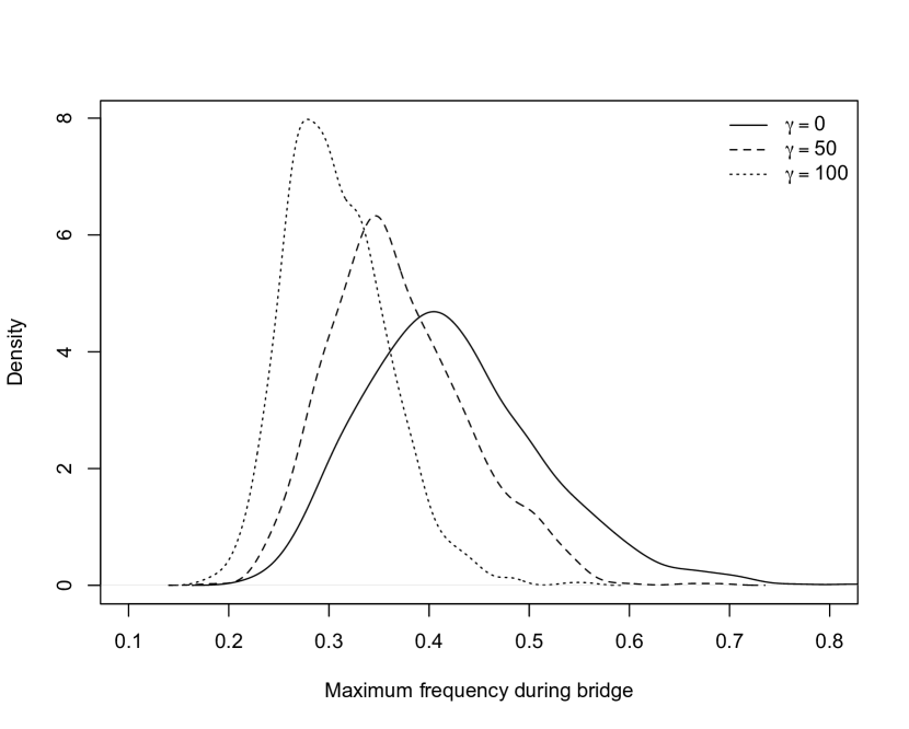
Figure 7.3. Densities of the maximum in a $0$ to $0$ bridge over the time interval $[0,T]=[0,0.1]$ for the selection strengths $\gamma=0$, $\gamma=50$ and $\gamma=100$.

Being able to sample Wright-Fisher bridge paths makes it very easy to numerically approximate the distribution and expectation of various functionals of the path. As an example, Figure 7.3 shows the density of the maximum in a bridge from $x=0$ to $z=0$ over the time interval $[0,T]=[0,0.1]$ for $\gamma=0$, $\gamma=50$ and $\gamma=100$. Note that the maximum in the bridge decreases as the strength of selection increases, and also becomes more tightly concentrated around its expectation.

To gain a more quantitative understanding of the extent to which a bridge for an allele experiencing natural selection looks different from the bridge for a neutral allele, it is possible to compute the Radon-Nikodym derivative (i.e. the likelihood ratio) of the distribution under selection against the distribution under neutrality. Using an argument similar to that which led to (4.8), the likelihood ratio is

(4.13) $$\frac{d\mathbb{P}_{\gamma}}{d\mathbb{P}_{0}}(\omega)\propto\exp\left\{-\frac{1}{8}\int_{0}^{T}\gamma^{2}\sin^{2}(\omega_{t})\,dt\right\},$$

where the constant of proportionality only depends on the endpoints. A few things are immediately evident from (4.13). First of all, the likelihood ratio does not depend on the sign of the selection coefficient, only the magnitude. This is analogous to the result Maruyama (1974) that, conditioned on eventual fixation, the sign of the selection coefficient is irrelevant to the distribution of the Wright-Fisher diffusion path. Also apparent is that bridges with strong natural selection will be more likely to be found near the boundary than bridges under neutrality. Finally, because $0\leq\sin^{2}(x)\leq 1$, we see that, very loosely, a bridge will look approximately neutral if

(4.14) $$\frac{1}{8}\gamma^{2}T\approx 0.$$

5. Discussion

We have examined the behavior of Wright-Fisher diffusion bridges under both neutral models and models with genic selection. Although various conditioned Wright-Fisher diffusions have been studied in the past, Wright-Fisher diffusions conditioned to obtain a specific value at a predetermined time have not been studied extensively. We have elucidated some of the properties of Wright-Fisher bridges using a combination of analytical theory and simulations.

In contrast to Brownian motion with drift, for which the distribution of a bridge does not depend on the magnitude of the drift coefficient, the distribution of a Wright-Fisher bridge does depend on the magnitude of the selection coefficient. As one might expect, bridges under strong selection are more constrained than neutral bridges. This can clearly be seen in Figure 7.2, in which the bridge with $\gamma=0$ has a broad range, but when $\gamma=100$ the paths of the bridge are highly likely to be confined near the boundary at $0$ until quite late in the bridge. A similar conclusion can be drawn from Figure 7.3 which shows the density of the maximum in a bridge from $0$ to $0$ over the time interval $[0,T]=[0,0.1]$. The expected maximum of a neutral bridge is much higher than one with strong selection, and there is significantly more variance about that maximum under neutrality.

Much of the behavior of Wright-Fisher bridges under selection can be understood in terms of the likelihood ratio (4.13). Because $\sin(x)$ takes its smallest values for $x\approx 0$ and $x\approx\pi$, very strong selection will confine a bridge of the transformed process $Y$ to near these boundaries. Intuitively, this is because the Wright-Fisher diffusion has the largest magnitude of drift and diffusion coefficients at $x=0.5$, and thus the diffusion moves “faster” when it is away from the boundaries $0$ and $1$. In order for a diffusion with a large selection coefficient to reach an interior point after a large amount of time, it must spend most of that time near the boundary.

However, these differences between selection and neutrality are mostly apparent in cases of extreme selection coefficients or very long times. This has important implications for maximum likelihood inference of selection coefficients from allele frequency time series. Because the realizations are likely to be quite similar for a selected allele and a neutral allele when the selection coefficient is moderate, most of the information about the selection coefficient comes from the end-points. Therefore, in many cases increasing the time-density of samples may not provide much additional information about the selection coefficient. Because many allelic time-series are obtained via costly ancient DNA techniques, this is an important consideration for the many researchers who are interested in the history of selection acting on a particular allele.

In addition to results directly concerning bridges, we have made several technical advances in the analysis of the Wright-Fisher diffusion. We have developed the theory of first passage times of a neutral Wright-Fisher diffusion starting from low frequency and we were able to provide a closed-form for the density of the maximum in a neutral bridge that goes from $0$ to $0$.

While our rejection sampling scheme is similar to that of Beskos and Roberts (2005) in some regards, there are several differences. Primarily, we do not provide exact samples, in the sense that Beskos and Roberts (2005) does. Because we store a discrete representation of our proposal bridges in computer memory, the calculation of (4.8) is necessarily an approximation, and hence the samples are only approximate. However, Figure 7.1 shows that they are extremely accurate. Also, because we are concerned with a specific model, we used $4$-dimensional Bessel bridges, instead of Brownian bridges, in our proposal mechanism. This choice is superior for the Wright-Fisher diffusion because both the Bessel bridge and the Wright-Fisher bridge have boundaries at $0$ with asymptotically equivalent singularities in the drift coefficient, while the Brownian bridge can assume negative values and hence result an unacceptably high rejection rate when it is used as a proposal distribution. Ideally, we would sample from a proposal distribution that describes a diffusion that was also bounded above and had a suitable singularity in its drift coefficient at the upper boundary; however, we have not yet discovered an appropriate diffusion for which it is easy to sample the corresponding bridges. Finally, we make use of the “most likely” bridge path as a means of guiding samples of bridges that are likely to be extremely different from those generated by the $4$-dimensional Bessel bridge proposal distribution. This modification is akin to shifting the mean of a proposal distribution when doing rejection sampling of a $1$-dimensional random variable, and it greatly increases the efficiency of sampling.

6. Acknowledgments

The authors thank M. Slatkin and B. Peter for initial discussions that led to our interest in this topic.

7. Appendix

7.1. Eigenfunction expansions of the transition density

Eigenfunction expansions of the Wright-Fisher transition densities in the case of no mutation were first explored in Kimura [1957a]. The form given in Crow and Kimura [1970] is

$$f(x,y;t)=\sum_{i=1}^{\infty}\frac{4(2i+1)x(1-x)}{i(i+1)}C_{i-1}^{(3/2)}(1-2x)C_{i-1}^{(3/2)}(1-2y)e^{-\frac{1}{2}i(i+1)t},$$

where $C^{(3/2)}_{i-1}$ is the Gegenbauer polynomial $C_{i-1}^{(\lambda)}$ with $\lambda=3/2$.

An explicit formula for the Gegenbauer polynomial is

$$C_{n}^{(\lambda)}(x)=\sum_{k=0}^{\lfloor n/2\rfloor}(-1)^{k}\frac{\Gamma(n-k+\alpha)}{\Gamma(\alpha)k!(n-2k)!}(2x)^{n-2k}$$

The generating function for the sequence $(C_{n}^{\lambda})_{n=0}^{\infty}$ is

$$\sum_{n=0}^{\infty}C_{n}^{\lambda}(x)t^{n}=(1-2xt+t^{2})^{-\lambda}.$$

Note that

$$C_{n}^{\lambda}(1)=\frac{(2\lambda)_{(n)}}{n!},$$

and the right-hand side is $(n+1)(n+2)/2$ when $\lambda=3/2$.

The sequence of polynomials $(C_{n}^{(3/2)})_{n=0}^{\infty}$ satisfies the three-term recurrence

$$nC_{n}^{(3/2)}(x)=(2n+1)xC_{n-1}^{(3/2)}(x)-(n+1)C_{n-2}^{(3/2)}(x)$$

with initial conditions $C_{0}^{(3/2)}(x)=1$ and $C_{1}^{(3/2)}(x)=3x$. It is convenient in computations to use the scaled polynomials $P_{n}(x)=C_{n}^{(3/2)}(x)/C_{n}^{(3/2)}(1)$ which are bounded in modulus by unity on the interval $[-1,+1]$. The corresponding three-term recurrence for the sequence $(P_{n})_{n=0}^{\infty}$ is

$$(n+2)P_{n}(x)=(2n+1)xP_{n-1}(x)-(n-1)P_{n-2}(x)$$

with initial conditions $P_{0}(x)=1$ and $P_{1}(x)=x$.

The transition density written with the scaled polynomials is

$$f(x,y;t)=x(1-x)\sum_{i=1}^{\infty}(2i+1)i(i+1)P_{i-1}(r)P_{i-1}(s)e^{-\frac{1}{2}i(i+1)t}.$$

The asymptotic form of the transition density as $x\downarrow 0$ is

(7.1) $$f(x,y;t)\approx x\sum_{i=1}^{\infty}(2i+1)i(i+1)P_{i-1}(s)e^{-\frac{1}{2}i(i+1)t}$$

Also,

$$\lim_{x,y\downarrow 0}x^{-1}f(x,y;t)=\sum_{i=1}^{\infty}(2i+1)i(i+1)e^{-\frac{1}{2}i(i+1)t}.$$

We also use a form of the expansion that is formally equivalent to the one above – see Griffiths and Spanó [2010]. The expansion is

(7.2) $$f(x,y;t)=y^{-1}(1-y)^{-1}\sum_{n=2}^{\infty}e^{-\frac{1}{2}n(n-1)t}Q_{n}(x,y),$$

where

(7.3) $$Q_{n}(x,y):=(2n-1)\sum_{m=1}^{n}(-1)^{n-m}\frac{m_{(n-1)}}{m!(n-m)!}\xi_{m},$$

and

(7.4) $$\xi_{m}:=\sum_{l=1}^{m-1}\binom{m}{l}\frac{(m-1)!}{(l-1)!(m-l-1)!}(xy)^{l}[(1-x)(1-y)]^{m-l}.$$

Note that

$$\xi_{m}=xm(m-1)y(1-y)^{m-1}+O(x^{2})$$

as $x\downarrow 0$. Therefore,

(7.5) $$f(x,y;t)\sim x\sum_{n=2}^{\infty}e^{-\frac{1}{2}n(n-1)t}(2n-1)\sum_{m=1}^{n}(-1)^{n-m}\frac{m_{(n-1)}}{m!(n-m)!}m(m-1)(1-y)^{m-2},$$

which is equal to (3.9). To calculate

$$\lim_{x,y\downarrow 0}x^{-1}f(x,y;t)=2\sum_{l=2}^{\infty}h_{l}(t)$$

we observe that

(7.6) $$\sum_{m=1}^{n}(-1)^{n-m}\frac{m_{(n-1)}}{m!(n-m)!}m(m-1)=n(n-1).$$

Therefore,

(7.7) $$2\sum_{l=2}^{\infty}h_{l}(t)=\sum_{n=2}^{\infty}e^{-\frac{1}{2}n(n-1)t}(2n-1)n(n-1).$$

Figure 7.1. Q-Q plot showing the accuracy of the rejection sampling scheme. Theoretical quantiles were calculated using the method of Song and Steinrücken [2012] and sample quantiles are determined from $1000$ bridges simulated using the method described in the text. The bridge goes from $x=0.2$ to $z=0.7$ over the time interval $[0,T]=[0,0.1]$. The left panels correspond to $t=0.03$ and the right panels correspond to $t=0.07$. The top row corresponds to $\gamma=10$ and the bottom row to $\gamma=50$.

Figure 7.2. Plot showing the properties of bridge paths as the strength of selection increases. Each bridge is from $x=0.01$ to $z=0.8$ over the time interval $[0,T]=[0,0.1]$. The successive selection coefficients are $\gamma=0$, $\gamma=50$ and $\gamma=100$. For each selection coefficient, pointwise 0%, 25%, 50%, 75% and 100% quantiles are calculated. Solid line is the 50% quantile, dashed line indicates 25% and 75% quantiles, and the dotted line indicates 0% and 100% quantiles.

References

- Beskos and Roberts [2005] Alexandros Beskos and Gareth O. Roberts. Exact simulation of diffusions. Ann. Appl. Probab., 15(4):2422–2444, 2005. ISSN 1050-5164. doi: 10.1214/105051605000000485.
- Bollback et al. [2008] Jonathan P. Bollback, Thomas L. York, and Rasmus Nielsen. Estimation of 2Nes from temporal allele frequency data. Genetics, 179(1):497–502, May 2008. ISSN 0016-6731. doi: 10.1534/genetics.107.085019.
- Crow and Kimura [1970] James F. Crow and Motoo Kimura. An introduction to population genetics theory. Harper & Row Publishers, New York, 1970.
- Csáki et al. [1987] Endre Csáki, Antónia Földes, and Paavo Salminen. On the joint distribution of the maximum and its location for a linear diffusion. Ann. Inst. H. Poincaré Probab. Statist., 23(2):179–194, 1987. ISSN 0246-0203.
- Etheridge et al. [2006] Alison Etheridge, Peter Pfaffelhuber, and Anton Wakolbinger. An approximate sampling formula under genetic hitchhiking. Ann. Appl. Probab., 16:685–729, 2006. doi: 10.1214/105051606000000114.
- Ethier and Griffiths [1993] S. N. Ethier and R. C. Griffiths. The transition function of a Fleming-Viot process. Ann. Probab., 21(3):1571–1590, 1993. ISSN 0091-1798.
- Ewing and Hermisson [2010] Gregory Ewing and Joachim Hermisson. MSMS: a coalescent simulation program including recombination, demographic structure and selection at a single locus. Bioinformatics (Oxford, England), 26(16):2064–5, August 2010. ISSN 1367-4811. doi: 10.1093/bioinformatics/btq322.
- Feder et al. [2013] Alison Feder, Sergey Kryazhimskiy, and Joshua B. Plotkin. Identifying signatures of selection in genetic time series. arXiv preprint arXiv:1302.0452, 2013.
- Fisher [1922] R.A. Fisher. On the dominance ratio. Proceedings of the Royal Society of Edinburgh, 42:321–341, 1922.
- Griffiths and Spanó [2010] Robert C. Griffiths and Dario Spanó. Diffusion processes and coalescent trees. In Probability and mathematical genetics, volume 378 of London Math. Soc. Lecture Note Ser., pages 358–379. Cambridge Univ. Press, Cambridge, 2010.
- Hudson and Kaplan [1988] R. R. Hudson and N. L. Kaplan. The coalescent process in models with selection and recombination. Genetics, 120(3):831–40, November 1988. ISSN 0016-6731.
- Ikeda and Watanabe [1989] Nobuyuki Ikeda and Shinzo Watanabe. Stochastic differential equations and diffusion processes, volume 24 of North-Holland Mathematical Library. North-Holland Publishing Co., Amsterdam, second edition, 1989. ISBN 0-444-87378-3.
- Kaplan et al. [1989] N. L. Kaplan, R. R. Hudson, and C. H. Langley. The “hitchhiking effect” revisited. Genetics, 123(4):887–99, December 1989. ISSN 0016-6731.
- Kimura [1955] Motoo Kimura. Stochastic processes and distribution of gene frequencies under natural selection. In Cold Spring Harbor Symposia on Quantitative Biology, volume 20, pages 33–53. Cold Spring Harbor Laboratory Press, 1955.
- Kimura [1957a] Motoo Kimura. Some problems of stochastic processes in genetics. Ann. Math. Statist., 28:882–901, 1957a. ISSN 0003-4851.
- Kimura [1957b] Motoo Kimura. Some problems of stochastic processes in genetics. The Annals of Mathematical Statistics, pages 882–901, 1957b.
- Malaspinas et al. [2012] Anna-Sapfo Malaspinas, Orestis Malaspinas, Steven N. Evans, and Montgomery Slatkin. Estimating allele age and selection coefficient from time-serial data. Genetics, 192(2):599–607, 2012.
- Mardia et al. [1979] Kantilal Varichand Mardia, John T. Kent, and John M. Bibby. Multivariate analysis. Academic Press [Harcourt Brace Jovanovich Publishers], London, 1979. ISBN 0-12-471250-9. Probability and Mathematical Statistics: A Series of Monographs and Textbooks.
- Maruyama [1974] T. Maruyama. The age of an allele in a finite population. Genetical Research, 23(2):137–43, April 1974.
- Mathieson and McVean [2013] Iain Mathieson and Gil McVean. Estimating selection coefficients in spatially structured populations from time series data of allele frequencies. Genetics, 193(3):973–984, 2013.
- Nielsen et al. [2005] Rasmus Nielsen, Scott Williamson, Yuseob Kim, Melissa J. Hubisz, Andrew G. Clark, and Carlos Bustamante. Genomic scans for selective sweeps using SNP data. Genome Research, 15(11):1566–75, November 2005. ISSN 1088-9051. doi: 10.1101/gr.4252305.
- Peter et al. [2012] Benjamin M. Peter, Emilia Huerta-Sanchez, and Rasmus Nielsen. Distinguishing between selective sweeps from standing variation and from a de novo mutation. PLoS Genetics, 8(10):e1003011, 2012.
- Revuz and Yor [1999] Daniel Revuz and Marc Yor. Continuous martingales and Brownian motion, volume 293 of Grundlehren der Mathematischen Wissenschaften [Fundamental Principles of Mathematical Sciences]. Springer-Verlag, Berlin, third edition, 1999. ISBN 3-540-64325-7.
- Rogers and Williams [2000] L. C. G. Rogers and David Williams. Diffusions, Markov processes, and martingales. Vol. 2. Cambridge Mathematical Library. Cambridge University Press, Cambridge, 2000. ISBN 0-521-77593-0. Itô calculus, Reprint of the second (1994) edition.
- Slatkin and Excoffier [2012] Montgomery Slatkin and Laurent Excoffier. Serial founder effects during range expansion: a spatial analog of genetic drift. Genetics, 191(1):171–181, 2012.
- Smith and Haigh [1974] J. M. Smith and J. Haigh. The hitch-hiking effect of a favourable gene. Genetical Research, 23(1):23–35, February 1974.
- Song and Steinrücken [2012] Yun S. Song and Matthias Steinrücken. A simple method for finding explicit analytic transition densities of diffusion processes with general diploid selection. Genetics, 190(3):1117–1129, 2012. doi: 10.1534/genetics.111.136929.
- Steinrücken et al. [2012] Matthias Steinrücken, Y.X. Wang, and Yun S. Song. An explicit transition density expansion for a multi-allelic wright–fisher diffusion with general diploid selection. Theoretical Population Biology, 2012.
- Teshima and Innan [2009] Kosuke M. Teshima and Hideki Innan. mbs: modifying Hudson’s ms software to generate samples of DNA sequences with a biallelic site under selection. BMC Bioinformatics, 10:166, January 2009. ISSN 1471-2105. doi: 10.1186/1471-2105-10-166.
- Wright [1931] S. Wright. Evolution in Mendelian Populations. Genetics, 16(2):97–159, March 1931. ISSN 0016-6731.